Stabilization-free HHO a posteriori error control

Abstract

The known a posteriori error analysis of hybrid high-order methods (HHO) treats the stabilization contribution as part of the error and as part of the error estimator for an efficient and reliable error control. This paper circumvents the stabilization contribution on simplicial meshes and arrives at a stabilization-free error analysis with an explicit residual-based a posteriori error estimator for adaptive mesh-refining as well as an equilibrium-based guaranteed upper error bound (GUB). Numerical evidence in a Poisson model problem supports that the GUB leads to realistic upper bounds for the displacement error in the piecewise energy norm. The adaptive mesh-refining algorithm associated to the explicit residual-based a posteriori error estimator recovers the optimal convergence rates in computational benchmarks.

1 Introduction

Hybrid high-order methods (HHO) were introduced in Di-Pietro.Ern:15 ; Di-Pietro.Ern.ea:14 and are examined in the textbooks DiPietroDroniou2020 ; ern_finite_2021-2 as a promising class of flexible nonconforming discretization methods for partial differential equations that involve a parameter-free stabilization term for the link between the volume and skeletal variables.

1.1 Known a posteriori error estimator

The a priori error analysis of HHO involves the stability terms in extended norms as part of the methodology and motivated a first explicit residual-based a posteriori error estimator in DiPietroDroniou2020 with a reformulation of the stabilization in the upper bound. Let $s_{h}(u_{h},u_{h})$ denote the stabilization at the discrete solution $u_{h}\in V_{h}$ and let the (elliptic) reconstruction $Ru_{h}$ of $u_{h}$ denote a piecewise polynomial of degree at most $k+1$ that approximates $u\in H^{1}(\Omega)$, cf. (2) and Section 3 below for further details. Then a possible error term reads

$$\textup{total error}^{2}:=\|\nabla_{\textup{pw}}(u-Ru_{h})\|_{L^{2}(\Omega)}^{2}+s_{h}(u_{h},u_{h}).$$ (1)

It is disputable if $s_{h}(u_{h},u_{h})\geq 0$ is an error contribution, but if the total error includes $s_{h}(u_{h},u_{h})$ (or an equivalent form), then the error estimator may also include this term (or a computable equivalent) for a reliable and efficient a posteriori error control. Amongst the many skeletal schemes like (nonconforming) virtual elements, hybridized (weak) discontinuous Galerkin schemes et al., the HHO methodology has a clear and efficacious stabilization

$$s_{h}(v_{h},w_{h})\coloneqq\sum_{T\in\mathcal{T}}\sum_{F\in\mathcal{F}(T)}h_{F}^{-1}\langle S_{TF}v_{h},S_{TF}w_{h}\rangle_{L^{2}(F)}$$ (2)

with the abbreviation $S_{TF}v_{h}\coloneqq\Pi_{F,k}\left(v_{\mathcal{T}}+(1-\Pi_{T,k})Rv_{h}\right)|_{T}-v_{\mathcal{F}}|_{F}$ for $v_{h}=(v_{\mathcal{T}},v_{\mathcal{F}})\in V_{h}$ in terms of the $L^{2}$ projections $\Pi_{K,k}$ onto polynomials of degree at most $k$ on a facet or simplex $K\in\mathcal{F}\cup\mathcal{T}$ of diameter $h_{K}=\mathrm{diam}(K)$; cf. Subsection 1.4 for further details. The original residual-based estimator $\eta_{\rm HHO}$ from the textbook DiPietroDroniou2020 for the Poisson model problem $-\Delta u=f$ includes (2) and an interpolation $\mathcal{A}Ru_{h}\in V$ of $Ru_{h}$ by nodal averaging in

$$\eta_{\rm HHO}^{2}=\ \|h_{\mathcal{T}}(1-\Pi_{0})(f+{\Delta}_{\rm pw}Ru_{h})\|_{L^{2}(\Omega)}^{2}+\|\nabla_{{\rm pw}}(1-\mathcal{A})Ru_{h}\|_{L^{2}(\Omega)}^{2}$$

$$+s_{h}(u_{h},u_{h}).$$

(Multiplicative constants are undisplayed in this introduction for simplicity.) The results from Theorem 4.3 and 4.7 in DiPietroDroniou2020 show reliability and efficiency for the total error (1) and piecewise polynomial source terms $f\in P_{k+1}(\mathcal{T})$,

$$\text{total error}^{2}\approx\eta_{\rm HHO}^{2}.$$

1.2 Stabilization-free a posteriori error control

There are objections against the double role of $s_{h}(u_{h},u_{h})$ on both sides of the efficiency and reliability estimate. First, the term $s_{h}(u,u_{h})$ may dominate both sides of the error estimate. In other words, the total error might be equivalent to $s_{h}(u_{h},u_{h})$, but the quantity of interest may exclusively be

$$\textup{error}^{2}:=\|\nabla_{\textup{pw}}(u-Ru_{h})\|_{L^{2}(\Omega)}^{2}.$$

Second, since the stabilization (2) incorporates a negative power of the mesh-size, a reduction property for local refinements remains unclear but is inevitable in the proofs of optimal convergence of an adaptive algorithm bertrand_opt ; carstensen_axioms_2014 . This paper, therefore, asks a different question about the control of the error without the stabilization term (2) in the upper bound and introduces two stabilization-free error estimators (multiplicative constants are undisplayed)

$$\eta_{\text{res}}^{2}=\ \|h_{\mathcal{T}}(f+{\Delta}_{\rm pw}Ru_{h})\|_{L^{2}(\Omega)}^{2}+\sum_{F\in{\mathcal{F}}}h_{F}\|[\nabla_{{\rm pw}}Ru_{h}]_{F}\|_{L^{2}(F)}^{2},$$

$$\eta_{\text{eq},p}^{2}=\ \mathrm{osc}_{k+p}^{2}(f,\mathcal{T})+\|Q_{p}-\nabla_{\rm pw}Ru_{h}\|_{L^{2}(\Omega)}^{2}+\|\nabla_{{\rm pw}}(1-\mathcal{A})Ru_{h}\|_{L^{2}(\Omega)}^{2}$$

for some parameter $p\in\mathbb{N}_{0}$. The explicit residual-based a posteriori error estimator $\eta_{\rm res}$ follows from the a posteriori methodology in the spirit of b9ffd40a ; c6537ecf ; 5be62542 ; normOfdGrad4Hdiv2015ccdpas with a piecewise volume residual $f+\Delta_{\rm pw}Ru_{h}$ and the jumps $[\nabla_{{\rm pw}}Ru_{h}]_{F}$ across a facet $F$ (on the boundary this is only the tangential component of $\nabla_{{\rm pw}}Ru_{h}$). The equilibrated error estimator $\eta_{\mathrm{eq},p}$ includes the post-processed quantity $Q_{p}\in RT_{k+p}(\mathcal{T})$ in the space $RT_{k+p}(\mathcal{T})$ of Raviart-Thomas functions of degree $k+p$ for $p\in\mathbb{N}_{0}$ and the nodal average $\mathcal{A}Ru_{h}\in S^{k+1}_{0}(\mathcal{T})$ of $Ru_{h}$. The main results establish reliability and efficiency

$$\text{error}^{2}+\mathrm{osc}_{k-1}^{2}(f,\mathcal{T})\lesssim\eta_{\rm res}^{2}\approx\eta_{\mathrm{eq},p}^{2}\lesssim\text{error}^{2}+\mathrm{osc}_{q}^{2}(f,\mathcal{T})$$

for any $p,q\in\mathbb{N}_{0}$ up to data-oscillations $\mathrm{osc}_{q}^{2}(f,\mathcal{T})\coloneqq\|h_{\mathcal{T}}(1-\Pi_{q})f\|^{2}_{L^{2}(\Omega)}$ of the source term $f\in L^{2}(\Omega)$ and without any stabilization terms. Computational benchmarks with adaptive mesh-refinement driven by any of these estimators provide numerical evidence for optimal convergence rates.

1.3 Further contributions and outline

The higher-order Crouzeix-Raviart finite element schemes are complicated at least in 3D Ciarlet2018 and then the HHO methodology is an attractive alternative even for simplicial triangulations with partly unexpected advantages like the computation of higher-order guaranteed eigenvalue bounds CEP21 . Higher convergence rates rely on an appropriate adaptive mesh-refining algorithm and hence stabilization-free a posteriori error estimators are of particular interest. The recent paper daveiga2021adaptive establishes the latter for virtual elements with an over-penalization strategy as an extension of bonito_quasi-optimal_2010 for the discontinuous Galerkin schemes. A disadvantage is the quantification of the restriction on the stabilization parameter in practise and poor condition for larger parameters. The stabilization-free a posteriori error control in this paper is based on two observations for the HHO schemes on simplicial triangulations. First, the $P_{1}$-conforming finite element functions let the stabilization vanish and, second, the divergence-free lowest-order Raviart-Thomas functions are $L^{2}$ perpendicular to the piecewise gradients $\nabla_{{\rm pw}}Ru_{h}$. In fact, those two fairly general properties lead in Section 2 to a reliable explicit residual-based a posteriori error estimator. In contrast to the simplified introduction above, the paper also focuses on multiplicative constants that lead to the GUB

$$\textup{error}\leq\eta_{\rm res}\quad\text{and}\quad\textup{error}\leq\eta_{\mathrm{eq},p};$$

cf. Table 1 for explicit quantities and Theorem 2.1 and Theorem 4.1 for further details.

$\omega_{\rm max}$	$\pi$	$3\pi/2$	$2\pi$
$M_{\rm bd}$	4	6	8
$c_{\rm apx}$	2.9568	6.4642	11.3771
$C_{\rm st}$	26.0893	55.8498	97.5374
$C_{1}$	2.9718	6.4710	11.3810
$C_{2}$	7.0495	15.2341	26.7317

Table 1: Explicit constants $C_{\ref{cnst:C1}},C_{\rm st},C_{\ref{cnst:C2}}$ for right-isosceles triangles with respect to the maximum interior angle $\omega_{\rm max}$ of the polygonal domain $\Omega$.

Numerical comparisons of $\eta_{\rm HHO}$ with $\eta_{\rm res}$ and $\eta_{\mathrm{eq},p}$ favour the latter. Section 2 identifies general building blocks of the a posteriori error analysis for discontinuous schemes with emphasis on explicit constants. An application to HHO leads to the new stabilization-free residual-based estimator $\eta_{\rm res}$ in Section 3. The alternative stabilization-free error estimator $\eta_{\mathrm{eq},p}$ follows from an equilibration strategy plus post-processing in Section 4. This paper also contributes to the HHO literature a local equivalence of two stabilizations and the efficiency of the stabilization terms up to data-oscillations in extension of ErnZanotti2020 . Numerical comparisons of the different error estimators and an error estimator competition for guaranteed error control of the piecewise energy norm in 2D conclude this paper in Section LABEL:sec:Numerical_results. Three computational benchmarks provide striking numerical evidences for the optimality of the associated adaptive algorithms. The appendix provides algorithmic details on the computation of the post-processed contribution $\|Q_{p}-\nabla_{{\rm pw}}Ru_{h}\|_{L^{2}(\Omega)}$ in $\eta_{{\rm eq},p}$.

1.4 Overall notation

Standard notation for Sobolev and Lebesgue spaces and norms apply with $\|\bullet\|\coloneqq\|\bullet\|_{L^{2}(\Omega)}$ and $|\!|\!|\bullet|\!|\!|\coloneqq\|\nabla\bullet\|_{L^{2}(\Omega)}$. In particular, $H(\operatorname*{div},\Omega)$ is the space of Sobolev functions with weak divergence in $L^{2}(\Omega)$ and $H(\operatorname*{div}=0,\Omega)$ contains only divergence-free functions in $H(\operatorname*{div},\Omega)$. Throughout this paper, $\mathcal{T}$ denotes a shape-regular triangulation of the polyhedral bounded Lipschitz domain $\Omega\subset\mathbb{R}^{n}$ into $n$-simplices with facets $\mathcal{F}$ (edges for $n=2$ and faces for $n=3$) and vertices $\mathcal{V}$. Let $\mathcal{F}(\Omega)$ (resp. $\mathcal{V}(\Omega)$) denote the set of interior facets (resp. vertices) and $\mathcal{F}(\partial\Omega)\coloneqq\mathcal{F}\setminus\mathcal{F}(\partial\Omega)$ (resp. $V(\partial\Omega)\coloneqq\mathcal{V}\setminus\mathcal{V}(\Omega)$). Given $v\in\Omega\to\mathbb{R}^{n}$ and $w:\Omega\to\mathbb{R}^{2n-3}$, let $\operatorname*{curl}v\coloneqq\partial_{1}v_{2}-\partial_{2}v_{1}$ and $\operatorname*{Curl}w\coloneqq(\partial_{2}w,-\partial_{1}w)^{t}$ if $n=2$ and $\operatorname*{curl}v\coloneqq(\partial_{2}v_{3}-\partial_{3}v_{2},\partial_{3}v_{1}-\partial_{1}v_{3},\partial_{1}v_{2}-\partial_{2}v_{1})^{t}$ and $\operatorname*{Curl}w\coloneqq\operatorname*{curl}w$ if $n=3$. For $s\in\mathbb{R}$, let $H^{s}(\mathcal{T})$, $H(\operatorname*{div},\mathcal{T})$, and $H(\operatorname*{curl},\mathcal{T})$ denote the space of piecewise Sobolev functions with restriction to $T\in\mathcal{T}$ in $H^{s}(T)$, $H(\operatorname*{div},T)$, and $H(\operatorname*{curl},T)$. To simplify notation, $H^{s}(K)$ abbreviates $H^{s}(\mathrm{int}(K))$ for the open interior $\mathrm{int}(K)$ of a compact set $K$. The $L^{2}$-scalar product reads $(\bullet,\bullet)_{L^{2}(\omega)}$ for volumes $\omega\subseteq\Omega$ and $\langle\bullet,\bullet\rangle_{L^{2}(\gamma)}$ for surfaces $\gamma\subset\overline{\Omega}$ of co-dimension one; the same symbol applies to scalars and to vectors. For $V\coloneqq H^{1}_{0}(\Omega)$ and $V^{*}\coloneqq H^{-1}(\Omega)$, let $\langle\bullet,\bullet\rangle$ denote the duality-brackets in $V^{*}\times V$ for the dual space $V^{*}$ of $V$ equipped with the operator norm $|\!|\!|F|\!|\!|_{*}\coloneqq\sup_{v\in V\setminus\{0\}}|Fv|/|\!|\!|v|\!|\!|$ for $F\in V^{*}$.

Define the energy scalar product $a(v,w)\coloneqq(\nabla v,\nabla w)_{L^{2}(\Omega)}$ for $v,w\in H^{1}(\Omega)$ and its piecewise version $a_{{\rm pw}}(v,w)=(\nabla_{{\rm pw}}v,\nabla_{{\rm pw}}w)_{L^{2}(\Omega)}$ for $v,w\in H^{1}(\mathcal{T})$. The latter induces the seminorm $|\!|\!|\bullet|\!|\!|_{\rm pw}\coloneqq a_{\rm pw}(\bullet,\bullet)^{1/2}$ in $H^{1}(\mathcal{T})$. Here and throughout the paper, $\nabla_{{\rm pw}}$, ${\operatorname*{div}}_{\rm pw}$, $\operatorname*{curl}_{\rm pw}$, ${\Delta}_{\rm pw}$, denote the piecewise evaluation of the differential operators $\nabla$, $\operatorname*{div}$, $\operatorname*{curl}_{\rm pw}$, $\Delta$ without explicit reference to the underlying shape-regular triangulation $\mathcal{T}$.

The vector space $P_{k}(K)$ of polynomials of degrees at most $k\in{\mathbb{N}}_{0}$ over a facet or simplex $K\in\mathcal{F}\cup\mathcal{T}$ defines the piecewise polynomial spaces

$$P_{k}(\mathcal{T}) \coloneqq\{p\in L^{2}(\Omega)\ :\ p_{|T}\in P_{k}(T)\text{ for all }T\in\mathcal{T}\},$$

$$P_{k}(\mathcal{F}) \coloneqq\{p\in L^{2}(\mathcal{F})\ :\ p_{|F}\in P_{k}(F)\text{ for all }F\in\mathcal{F}\}\$$

and the space of piecewise Raviart-Thomas functions

$$RT_{k}^{\rm pw}(\mathcal{T})\coloneqq P_{k}(\mathcal{T};\mathbb{R}^{n})+xP_{k}(\mathcal{T}).$$

The associated $L^{2}$ projections read $\Pi_{K,k}:L^{2}(\Omega)\to P_{k}(K),\Pi_{k}:L^{2}(\Omega)\rightarrow P_{k}(\mathcal{T}),$ and $\Pi_{\mathcal{F},k}:L^{2}(\Omega)\rightarrow P_{k}(\mathcal{F})$ with the convention $\Pi_{-1}\coloneqq 0$. Abbreviate $S^{k+1}_{0}(\mathcal{T})\coloneqq P_{k+1}(\mathcal{T})\cap V$ and $RT_{k}(\mathcal{T})\coloneqq RT^{\rm pw}_{k}(\mathcal{T})\cap H(\operatorname*{div},\Omega)$ for all $k\in\mathbb{N}_{0}$. The piecewise constant mesh-size function $h_{\mathcal{T}}\in P_{0}(\mathcal{T})$ satisfies $h_{\mathcal{T}|T}\coloneqq h_{T}$ for $T\in\mathcal{T}$ with the diameter $h_{K}\coloneqq\mathrm{diam}(K)\in P_{0}(K)$ of $K\in\mathcal{F}\cup\mathcal{T}$.

If not explicitly stated otherwise, constants are independent of the mesh-size in the triangulation but may depend on the shape-regularity and on the polynomial degree $k$. The abbreviation $A\lesssim B$ hides a generic constant $C$ (independent of the mesh-size) in $A\leq C\;B$; $A\approx B$ abbreviates $A\lesssim B\lesssim A$.

2 Foundations of the a posteriori error analysis

This section investigates general building blocks of the a posteriori error analysis and revisits arguments from b9ffd40a ; c6537ecf ; 5be62542 ; normOfdGrad4Hdiv2015ccdpas with emphasis on multiply connected domains $\Omega\subset\mathbb{R}^{n}$ for $n=2,3$. The general setting of this section results in reliability for an error estimator that is applicable beyond the HHO methodology. Consider the weak solution $u\in V=H^{1}_{0}(\Omega)$ to the Poisson model problem $-\Delta u=f$ a.e. in $\Omega$ and $u=0$ on $\partial\Omega$ for a given source $f\in L^{2}(\Omega)$; i.e., $u\in V$ satisfies

$$a(u,v)=(f,v)_{L^{2}(\Omega)}\quad\text{for all }v\in V.$$ (3)

An approximation ${G}\in L^{2}(\Omega;\mathbb{R}^{n})$ of the gradient $\nabla u\in H(\operatorname*{div},\Omega)$ gives rise to the residual $f+\operatorname*{div}{G}\in V^{*}=H^{-1}(\Omega)$ seen as a linear functional on $V$, i.e.,

$$\langle f+\operatorname*{div}{G},\varphi\rangle:=(f,\varphi)_{L^{2}(\Omega)}-({G},\nabla\varphi)_{L^{2}(\Omega)}\quad\text{for all }\varphi\in V.$$

Let $\nu_{T}$ denote the unit outer normal along the boundary $\partial T$ of each simplex $T\in\mathcal{T}$ and fix the orientation of a unit normal $\nu_{F}=\pm\nu_{T}$ for each facet $F\in\mathcal{F}(T)$ of $T$ such that it matches the outer unit normal $\nu$ of $\partial\Omega$ at the boundary. The jump $[{G}]_{F}$ of a piecewise function in $m\in{\mathbb{N}}$ components ${G}\in H^{1}(\mathcal{T};\mathbb{R}^{m})$ reads $[{G}]_{F}\coloneqq{G}_{|T_{+}}-{G}_{|T_{-}}$ on interior facets $F=T_{+}\cap T_{-}\in\mathcal{F}(\Omega)$ (with $T_{\pm}$ labelled such that $\nu_{T_{+}|F}=\nu_{F}=-\nu_{T_{-}|F})$ and $[{G}]_{F}\coloneqq{G}$ on the boundary $F\in\mathcal{F}(\partial\Omega)$. The main result of this section establishes the residual-based error estimator

$$\eta^{2}(\mathcal{T},{G})\coloneqq \left(C_{\ref{cnst:C1}}\|h_{\mathcal{T}}(f+{\operatorname*{div}}_{\rm pw}{G})\|+C_{\ref{cnst:C2}}\sqrt{\sum_{F\in{\mathcal{F}}(\Omega)}\ell(F)\|[{G}]_{F}\cdot\nu_{F}\|_{L^{2}(F)}^{2}}\right)^{2}$$ (4)

$$+C_{\rm H}^{2}\left(C_{\ref{cnst:C1}}\|h_{\mathcal{T}}{\operatorname*{curl}}_{\rm pw}{G}\|+C_{\ref{cnst:C2}}\sqrt{\sum_{F\in{\mathcal{F}}}\ell(F)\|[{G}]_{F}\times\nu_{F}\|_{L^{2}(F)}^{2}}\right)^{2}$$

as a GUB $\|\nabla u-{G}\|\leq\eta(\mathcal{T},{G})$ under minimal assumptions on the approximation ${G}\in H^{1}(\mathcal{T};\mathbb{R}^{n})\subset L^{2}(\Omega;\mathbb{R}^{n})$. The constants $C_{1}$, $C_{2}$, and $C_{H}$ (or upper bounds thereof) are computable; cf. Table 1 for an example in 2D with details in Example 1 at the end of Section 2. The first assumption is a weakened discrete solution property

$$({G},\nabla w_{C})_{L^{2}(\Omega)}=(f,w_{C})_{L^{2}(\Omega)}\quad\text{for all }w_{C}\in S_{0}^{1}(\mathcal{T}).$$ (5)

The second assumption is the orthogonality to the lowest-order divergence-free Raviart-Thomas functions

$$({G},r)_{L^{2}(\Omega)}=0\quad\text{for all }r\in RT_{0}(\mathcal{T})\cap H(\operatorname*{div}=0,\Omega).$$ (6)

Theorem 2.1 (residual-based GUB)

Suppose that ${G}\in H^{1}(\mathcal{T};\mathbb{R}^{n})$ and $f\in L^{2}(\Omega)$ satisfy (5)–(6). Then the error estimator $\eta(\mathcal{T},{G})$ from (4) is a GUB

$$\|\nabla u-{G}\|\leq\eta(\mathcal{T},{G})$$

of the error $\|\nabla u-{G}\|$ for the solution $u\in V$ to (3). The constants $C_{\rm 1},C_{2},C_{\rm H}$ exclusively depend on $\Omega$ and the shape-regularity of $\mathcal{T}$.

The remaining parts of this section are devoted to the proof of Theorem 2.1 and the computation of (upper bounds of) the constants $C_{\rm 1},C_{\rm 2}$, and $C_{\rm H}$ in (4). The point of departure is the subsequent decomposition that appears necessary in the nonconforming and mixed finite element a posteriori error analysis. It leads to a split of the error $\|\nabla u-{G}\|$ into some divergence part and some consistency part.

Lemma 1 (decomposition)

Any $v\in V$ and ${G}\in L^{2}(\Omega;\mathbb{R}^{n})$ satisfy the decomposition

$$\|\nabla v-{G}\|^{2}=|\!|\!|v-w|\!|\!|^{2}+\|{G}-\nabla w\|^{2}$$ (7)

with the (unique) minimizer $w\in V$ of the distance

$$\delta:=\min_{\varphi\in V}\|{G}-\nabla\varphi\|$$

of ${G}$ to the gradients $\nabla V$ of Sobolev functions. The solution $u\in V$ to (3) satisfies

$$\mu\coloneqq \;|\!|\!|f+\operatorname*{div}{G}|\!|\!|_{*}=|\!|\!|u-w|\!|\!|$$ and

$$\|\nabla u-{G}\|^{2}= \;|\!|\!|f+\operatorname*{div}{G}|\!|\!|_{*}^{2}+\|{G}-\nabla w\|^{2}=\mu^{2}+\delta^{2}.$$ (8)

Proof

The minimizer $w\in V$ of $\|{G}-\nabla\varphi\|$ among $\varphi\in V$ satisfies the variational formulation $a(w,\varphi)_{L^{2}(\Omega)}=({G},\nabla\varphi)_{L^{2}(\Omega)}$ for all $\varphi\in V$. (Notice that $w$ is the unique weak solution to the Poisson model problem $-\Delta w=-\operatorname*{div}{G}\in V^{*}$.) In particular, ${G}-\nabla w$ is $L^{2}$ orthogonal onto $\nabla V$ and the Pythagoras theorem proves (7). Given $\varphi\in V$ with $|\!|\!|\varphi|\!|\!|=1$, the orthogonality of ${G}-\nabla w$ to $\nabla\varphi$ and (3) show

$$a(u-w,\varphi)_{L^{2}(\Omega)}=(\nabla u-{G},\nabla\varphi)_{L^{2}(\Omega)}=\langle f+\operatorname*{div}{G},\varphi\rangle$$ (9)

with the duality brackets $\langle\bullet,\bullet\rangle$ in $V^{*}\times V$. Since the supremum of (9) over all $\varphi\in V$ with $|\!|\!|\varphi|\!|\!|=1$ is equal to $|\!|\!|u-w|\!|\!|=|\!|\!|f+\operatorname*{div}{G}|\!|\!|_{*}$, this and (7) conclude the proof of (8). ∎

The split (7) of the error $\|\nabla u-{G}\|$ allows for and enforces a separate estimation of the equilibrium and consistency contribution in residual-based a posteriori error estimators.

In order to derive explicit constants, two lemmas are recalled. The first has a long tradition in the a posteriori error control in form of a Helmholtz decomposition on simply connected domains c43f5cd9 ; alonso1996error and introduces the constant $C_{\rm H}$ from Theorem 2.1. The following version includes the general case of multiply connected domains as in GirRav:86 for $n=2$ or $n=3$ dimensions and weak assumptions on a divergence-free function $\varrho\in H(\operatorname*{div}=0,\Omega)$.

Lemma 2 (Helmholtz-decomposition)

Suppose the divergence-free function $\varrho\in H(\operatorname*{div}=0,\Omega)$ is $L^{2}$ orthogonal onto $RT_{0}(\mathcal{T})\cap H(\operatorname*{div}=0,\Omega)$. Then there exists $\beta\in H^{1}(\Omega;\mathbb{R}^{N})$, $N=2n-3$, such that any $\beta_{C}\in S^{1}(\mathcal{T})^{N}$ satisfies

$$\|\varrho\|^{2}=\int_{\Omega}\varrho\cdot\mathrm{Curl}(\beta-\beta_{C})\ \mathrm{d}x\quad\text{and}\quad|\!|\!|\beta|\!|\!|\leq C_{\rm H}\,\|\varrho\|.$$ (10)

The constant $C_{\rm H}>0$ exclusively depends on $\Omega$.

Proof

The compact polyhedral boundary $\partial\Omega$ of the bounded Lipschitz domain $\Omega$ has $J+1$ connectivity components $\Gamma_{0},\dots,\Gamma_{J}$ for some finite $J\in\mathbb{N}_{0}$. Those connectivity components have a positive surface measure $|\Gamma_{j}|$ and a positive distance of each other. So the integral mean

$$\gamma_{j}:=\int_{\Gamma_{j}}\varrho\cdot\nu\,\ \mathrm{d}s/|\Gamma_{j}|$$

is well defined and depends continuously on $\varrho\in H(\operatorname*{div}=0,\Omega)$ in the sense that $|\gamma_{j}|\leq c_{1}\|\varrho\|$ (recall $\operatorname*{div}\varrho=0$) for each $j=0,\dots,J$ and $c_{1}>0$. This constant $c_{1}$ and the constants $c_{2},c_{3},c_{4}$ below exclusively depend on the domain $\Omega$. The finite real numbers $\gamma_{0},\dots,\gamma_{J}$ define the Neumann data for the harmonic function $z\in H^{1}(\Omega)/\mathbb{R}$ with

$$\Delta z=0\text{ in }\Omega\quad\text{and}\quad\partial z/\partial\nu=\gamma_{j}\text{ on }\Gamma_{j}\text{ for all }j=0,\dots,J.$$

The elliptic regularity theory for polyhedral domains lead to $z\in H^{1+\alpha}(\Omega)$ for some $\alpha>1/2$ and $c_{2}>0$ with $\|z\|_{H^{1+\alpha}(\Omega)}\leq c_{2}\,(|\gamma_{0}|+\dots+|\gamma_{J}|)$. The Raviart-Thomas interpolation operator defines a bounded linear operator on $H(\operatorname*{div},\Omega)\cap L^{p}(\Omega;\mathbb{R}^{n})$ for $p>2$. It is generally accepted that, for $\alpha>0$ and $\nabla z\in H(\operatorname*{div}=0,\Omega)\cap H^{\alpha}(\Omega;\mathbb{R}^{n})$, the Fortin interpolation $I_{\rm F}\nabla z\in RT_{0}(\mathcal{T})\cap H(\operatorname*{div}=0,\Omega)$ is well defined and $\|I_{\rm F}\nabla z\|\leq c_{3}\|\nabla z\|_{H^{\alpha}(\Omega)}$ follows for some $c_{3}>0$. The additional property $\nabla z\in L^{p}(\Omega;\mathbb{R}^{n})$ for some $p>2$ allows the definition of $\int_{F}\nabla z\cdot\nu_{F}\ \mathrm{d}s$ as a Lebesgue integral over a facet $F\in\mathcal{F}$. One consequence for the boundary facets is the vanishing integral

$$\int_{\Gamma_{j}}(\varrho-I_{\rm F}\nabla z)\cdot\nu\,\mathrm{d}s=0\quad\text{for all }j=0,\dots,J.$$

Since $\varrho-I_{\rm F}\nabla z\in H(\operatorname*{div}=0,\Omega)$ is divergence-free, Theorems 3.1 and 3.4 in GirRav:86 prove the existence of $c_{4}>0$ and $\beta\in H^{1}(\Omega;\mathbb{R}^{N})$ with

$$\varrho=I_{\rm F}\nabla z+\operatorname*{Curl}\beta\quad\text{and}\quad|\!|\!|\beta|\!|\!|\leq c_{4}\|\varrho-I_{\rm F}\nabla z\|.$$

Recall that $\varrho\perp I_{\rm F}\nabla z$ and $\varrho\perp\operatorname*{curl}\beta_{C}\in RT_{0}(\mathcal{T})\cap H(\operatorname*{div}=0,\Omega)$. This concludes the proof of (10) with $C_{\rm H}\coloneqq\sqrt{1+(c_{1}c_{2}c_{3}(1+J))^{2}}c_{4}$.∎

The subsequent version of the trace inequality on the facets $\mathcal{F}$ leads to the piecewise constant $\ell\in P_{0}(\mathcal{F})$ defined by

$$\ell(F)\coloneqq\begin{cases}{}(n+1)h_{T}^{2}|F|/|T|&\text{for }F\in\mathcal{F}(\partial\Omega)\cap\mathcal{F}(T),\\ (n+1)|F|/(h_{T_{+}}^{-2}|T_{+}|+h_{T_{-}}^{-2}|T_{-}|)&\text{for }F=\partial T_{+}\cap\partial T_{-}\in\mathcal{F}(\Omega).\end{cases}$$

Lemma 3 (trace inequality)

Any $f\in H^{1}(\Omega)$ satisfies

$$\sum_{F\in\mathcal{F}}\ell(F)^{-1}\left\|f\right\|_{L^{2}(F)}^{2}\leq\left\|h_{\mathcal{T}}^{-1}f\right\|^{2}+\frac{2C_{\rm tr}}{n}\left\|h_{\mathcal{T}}^{-1}f\right\|{\left|\kern-1.07639pt\left|\kern-1.07639pt\left|f\right|\kern-1.07639pt\right|\kern-1.07639pt\right|}$$

with the constant $C_{\rm tr}\coloneqq\max_{T\in\mathcal{T}}\max_{x\in T}|x-\mathrm{mid}(T)|/h_{T}<n/(n+1)$.

Proof

The center of inertia $\mathrm{mid}(T)=\sum_{j=0}^{n}P_{j}/(n+1)$ of the $n$-simplex $T=\mathrm{conv}\{P_{0},...,P_{n}\}\in\mathcal{T}$ and the $n+1$ faces $F_{j}=\mathrm{conv}\{P_{0},...,P_{j-1},P_{j+1},...,P_{n}\}\in\mathcal{F}(T)$ for $j=0,...,n$ give rise to the decomposition of $T$ into $n+1$ sub-simplices $T_{j}^{\prime}=\mathrm{conv}(F_{j},\mathrm{mid}(T))$ with volume $|T_{j}^{\prime}|=|T|/(n+1)$.

Standard arguments like the trace identity on $T_{j}^{\prime}\subset T$ (carstensen_explicit_2012, , Lemma 2.1) for $|f|^{2}\in W^{1,1}(T^{\prime})$ and a Cauchy inequality show

$$\frac{1}{|F_{j}|}\left\|f\right\|_{L^{2}(F_{j})}^{2}\leq\frac{1}{|T_{j}^{\prime}|}\left\|f\right\|_{L^{2}(T_{j}^{\prime})}^{2}+\frac{2}{n|T_{j}^{\prime}|}\max_{x\in T_{j}^{\prime}}|x-\mathrm{mid}(T)|\left\|f\right\|_{L^{2}({T_{j}^{\prime}})}\|\nabla f\|_{L^{2}(T^{\prime})}.$$

The distance $\max_{x\in T_{j}^{\prime}}|x-\mathrm{mid}(T)|=|P_{k}-\mathrm{mid}(T)|\leq C_{\rm tr}h_{T}$ is attained at a vertex $P_{k}$ for $k\in\{0,...,j-1,j+1,...,n\}$. Since the centroid $\mathrm{mid}(T)$ divides each median of $T$ in the ratio $n$ to $1$ and the length of each median is strictly bounded by $h_{T}$, the bound $C_{\rm tr}<n/(n+1)$ follows and cannot be improved in the absence of further assumptions on the shape of the simplex $T$. Since $|T_{j}^{\prime}|=|T|/(n+1)$, the previously displayed estimate leads to

$$\frac{|T|}{(n+1)h_{T}^{2}|F_{j}|}\left\|f\right\|_{L^{2}(F_{j})}^{2} \leq\left\|h_{T}^{-1}f\right\|_{L^{2}(T_{j}^{\prime})}^{2}+\frac{2C_{\rm tr}}{n}\left\|h_{T}^{-1}f\right\|_{L^{2}({T_{j}^{\prime}})}\|\nabla f\|_{L^{2}(T_{j}^{\prime})}.$$

Let $\mathcal{T}^{\prime}$ be the refinement of $\mathcal{T}$, obtained by replacing $T\in\mathcal{T}$ with $T_{0}^{\prime},...,T_{d}^{\prime}$ from above. The triangulation $\mathcal{T}^{\prime}$ allows for the facet based decomposition $\{\omega^{\prime}(F)\}_{F\in\mathcal{F}}$ of $\Omega$, where $\omega^{\prime}(F)$ is either the patch $\omega^{\prime}(F)=\mathrm{int}(T^{\prime}_{+}\cup T^{\prime}_{-})$ for an interior facet $F=T^{\prime}_{+}\cap T^{\prime}_{-}$ or $\omega^{\prime}(F)=\mathrm{int}(T^{\prime})$ for $F\in\mathcal{F}(\partial\Omega)\cap\mathcal{F}(T^{\prime})$. This establishes, for any $F\in\mathcal{F}$, the estimate

$$\ell(F)^{-1}\left\|f\right\|_{L^{2}(F)}^{2} \leq\left\|h_{\mathcal{T}}^{-1}f\right\|_{L^{2}(\omega^{\prime}(F))}^{2}+\frac{2C_{\rm tr}}{n}\left\|h_{\mathcal{T}}^{-1}f\right\|_{L^{2}(\omega^{\prime}(F))}\|\nabla f\|_{L^{2}(\omega^{\prime}(F))}.$$

Since the family $\{\omega^{\prime}(F):F\in\mathcal{F}\}$ has no overlap, the sum of the last displayed inequality over all $F\in\mathcal{F}$ and a Cauchy inequality conclude the proof of Lemma 3.∎

The next lemma utilizes a quasi-interpolation operator $J:H^{1}(\Omega)\to S^{1}(\mathcal{T})$ with the restriction $J(V)\subset S^{1}_{0}(\mathcal{T})$, e.g., $J=J_{1}\circ I_{NC}$ from (carstensen_constants_2018, , Section 5) with explicit constants for $n=2$, and the approximation and stability properties

$$\left\|h_{\mathcal{T}}^{-1}(\varphi-J\varphi)\right\| \leq C_{\ref{cnst:C1}}{\left|\kern-1.07639pt\left|\kern-1.07639pt\left|\varphi\right|\kern-1.07639pt\right|\kern-1.07639pt\right|}\quad\text{and}\quad{\left|\kern-1.07639pt\left|\kern-1.07639pt\left|\varphi-J\varphi\right|\kern-1.07639pt\right|\kern-1.07639pt\right|}\leq C_{\rm st}{\left|\kern-1.07639pt\left|\kern-1.07639pt\left|\varphi\right|\kern-1.07639pt\right|\kern-1.07639pt\right|}$$ (11)

for constants $C_{\ref{cnst:C1}}$ and $C_{\rm st}$ exclusively depending on the shape-regularity of $\mathcal{T}$. For the precise definition of $J_{1}$ and $I_{NC}$, we refer to (carstensen_constants_2018, , eq. (47) and Section 5). Recall the constant $C_{\rm tr}$ from Lemma 3 and set $C_{\ref{cnst:C2}}\coloneqq(C_{\ref{cnst:C1}}(C_{\ref{cnst:C1}}+2C_{\rm tr}C_{\rm st}\,/n))^{1/2}$.

Lemma 4 (equilibrium)

Suppose that ${G}\in H(\operatorname*{div},\mathcal{T})$ and $f\in L^{2}(\Omega)$ satisfy (5) and suppose $({G}|_{T})|_{F}\cdot\nu_{F}\in L^{2}(F)$ for all $F\in{\mathcal{F}}(T)$ and $T\in\mathcal{T}$. Then

$$|\!|\!|f+\operatorname*{div}{G}|\!|\!|_{*}\leq C_{\ref{cnst:C1}}\|h_{\mathcal{T}}(f+{\operatorname*{div}}_{\rm pw}{G})\|+C_{\ref{cnst:C2}}\sqrt{\sum_{F\in{\mathcal{F}}(\Omega)}\ell(F)\|[{G}]_{F}\cdot\nu_{F}\|_{L^{2}(F)}^{2}}.$$

Proof

Given $\varphi\in V$ with $|\!|\!|\varphi|\!|\!|=1$, set $\psi:=\varphi-\varphi_{C}$ for some quasi-interpolation $\varphi_{C}\coloneqq J\varphi\in S^{1}_{0}(\mathcal{T})$ with (11). Since (5) implies $\langle f+\operatorname*{div}{G},\varphi\rangle=\langle f+\operatorname*{div}{G},\psi\rangle$, a piecewise integration by parts and the collection of jump contributions show

$$\langle f+\operatorname*{div}{G},\varphi\rangle=(f+{\operatorname*{div}}_{\rm pw}{G},\psi)_{L^{2}(\Omega)}-\sum_{F\in{\mathcal{F}}(\Omega)}\langle[{G}]_{F}\cdot\nu_{F},\psi\rangle_{L^{2}(F)}.$$ (12)

The first bound follows from a Cauchy inequality and (11),

$$(f+{\operatorname*{div}}_{\rm pw}{G},\psi)_{L^{2}(\Omega)} \leq\|h_{\mathcal{T}}(f+{\operatorname*{div}}_{\rm pw}{G})\|\,\|h_{\mathcal{T}}^{-1}\psi\|$$ (13)

$$\leq C_{\ref{cnst:C1}}\|h_{\mathcal{T}}(f+{\operatorname*{div}}_{\rm pw}{G})\|\,|\!|\!|\varphi|\!|\!|.$$

The second bound additionally exploits the trace inequality of Lemma 3,

$$\sum_{F\in{\mathcal{F}}(\Omega)} \langle[{G}]_{F}\cdot\nu_{F},\psi\rangle_{L^{2}(F)}$$ (14)

$$\leq\sqrt{\sum_{F\in{\mathcal{F}}(\Omega)}\ell(F)\|[{G}]_{F}\cdot\nu_{F}\|_{L^{2}(F)}^{2}}\sqrt{\sum_{F\in{\mathcal{F}}(\Omega)}\ell(F)^{-1}\|\psi\|_{L^{2}(F)}^{2}}$$

$$\leq\sqrt{C_{\ref{cnst:C1}}^{2}+\frac{2C_{\rm tr}}{n}C_{\rm st}C_{\ref{cnst:C1}}}\sqrt{\sum_{F\in{\mathcal{F}}(\Omega)}\ell(F)\|[{G}]_{F}\cdot\nu_{F}\|_{L^{2}(F)}^{2}}$$

with ${\left|\kern-1.07639pt\left|\kern-1.07639pt\left|\varphi\right|\kern-1.07639pt\right|\kern-1.07639pt\right|}=1$ in the last step. Since (13)–(14) hold for all $\varphi\in V$ with $|\!|\!|\varphi|\!|\!|=1$, the supremum in (12) over all such $\varphi$ concludes the proof.∎

The final ingredient for the proof of Theorem 2.1 controls the second term $\delta$ in the decomposition of Lemma 1 for $\varrho\coloneqq{G}-\nabla w$. Recall $C_{\rm H}$ from Lemma 2 and $C_{\ref{cnst:C1}}$ from (11), and $C_{\ref{cnst:C2}}$ from page 9.

Lemma 5 (conformity)

Suppose the divergence-free function $\varrho\in H(\operatorname*{div}=0,\Omega)\cap H(\operatorname*{curl},\mathcal{T})$ is $L^{2}$ orthogonal onto $RT_{0}(\mathcal{T})\cap H(\operatorname*{div}=0,\Omega)$ and satisfies $(\varrho|_{T})|_{F}\times\nu_{F}\in L^{2}(F)$ for all $F\in{\mathcal{F}}(T)$ and $T\in T$. Then

$$C_{\rm H}^{-1}\|\varrho\|\leq C_{\ref{cnst:C1}}\|h_{\mathcal{T}}{\operatorname*{curl}}_{\rm pw}\varrho\|+C_{\ref{cnst:C2}}\sqrt{\sum_{F\in{\mathcal{F}}}\ell(F)\|[\varrho]_{F}\times\nu_{F}\|_{L^{2}(F)}^{2}}.$$

Proof

Lemma 2 provides $\beta\in H^{1}(\Omega;\mathbb{R}^{N})$ with (10) for a (component-wise) quasi-interpolation $\beta_{C}\in S^{1}(\mathcal{T})^{N}$ with (11) as in the proof of Lemma 4; set $\psi:=\beta-\beta_{C}$. A piecewise integration by parts and the collection of jump contributions shows

$$\|\varrho\|^{2}=\int_{\Omega}\varrho\cdot\operatorname*{Curl}(\beta-\beta_{C})dx=\int_{\Omega}\psi\cdot{\operatorname*{curl}}_{\rm pw}\varrho\,dx+\sum_{F\in{\mathcal{F}}}\int_{F}\psi[\varrho]_{F}\times\nu_{F}\,ds.$$

Stability and approximation properties of the quasi-interpolation (11) and the trace inequality of Lemma 3 eventually lead to

$$\left\|\varrho\right\|^{2} \leq C_{\ref{cnst:C1}}\left\|h_{\mathcal{T}}{\operatorname*{curl}}_{\rm pw}\varrho\right\||\!|\!|\beta|\!|\!|+C_{\ref{cnst:C2}}\sqrt{\sum_{F\in{\mathcal{F}}}\ell(F)\|[\varrho]_{F}\times\nu_{F}\|_{L^{2}(F)}^{2}}|\!|\!|\beta|\!|\!|.$$

In fact, the routine estimation with element and jump terms is completely analogous to the proof of Lemma 4 and leads to the same constants $C_{\ref{cnst:C1}},C_{\ref{cnst:C2}}$. This and $|\!|\!|\beta|\!|\!|\leq C_{\rm H}\|\varrho\|$ conclude the proof.∎

Proof (Theorem 2.1)

The trace of ${G}|_{T}\in H^{1}(T;\mathbb{R}^{n})$ is well defined on any facet $F\in\mathcal{F}(T)$ of the simplex $T\in\mathcal{T}$. Lemma 1 provides $w\in V=H^{1}_{0}(\Omega)$ with $\|\nabla u-{G}\|^{2}=|\!|\!|f+\operatorname*{div}{G}|\!|\!|_{*}^{2}+\|{G}-\nabla w\|^{2}$. Since ${G}$ satisfies (5), Lemma 4 establishes

$$|\!|\!|f+\operatorname*{div}{G}|\!|\!|_{*}\leq C_{\rm 1}\|h_{\mathcal{T}}(f+{\operatorname*{div}}_{\rm pw}{G})\|+C_{2}\sqrt{\sum_{F\in{\mathcal{F}}(\Omega)}\ell(F)\|[{G}]_{F}\cdot\nu_{F}\|_{L^{2}(F)}^{2}}.$$

The assumption (6) on ${G}$ and an integration by parts prove that Lemma 5 is applicable to $\varrho\coloneqq{G}-\nabla w\in H(\operatorname*{div}=0,\Omega)\cap H(\operatorname*{curl},\mathcal{T};\mathbb{R}^{n})$. Since $\operatorname*{curl}\nabla w=0$ and $\nabla w\times\nu=0$, this reveals

$$C_{\rm H}^{-1}\|{G}-\nabla w\|\leq C_{\rm 1}\|h_{\mathcal{T}}{\operatorname*{curl}}_{\rm pw}{G}\|+C_{2}\sqrt{\sum_{F\in{\mathcal{F}}}\ell(F)\|[{G}]_{F}\times\nu_{F}\|_{L^{2}(F)}^{2}}.$$

The above estimates together with the decomposition of Lemma 1 establish $\eta(\mathcal{T},{G})$ as a GUB for the error $\|\nabla u-{G}\|$. ∎

Example 1 (constants for right-isosceles triangles)

In two space dimensions, $\|\operatorname*{Curl}\bullet\|=|\!|\!|\bullet|\!|\!|$ and so $C_{\rm H}\leq 1$ for a simply connected domain $\Omega$ in Lemma 2. The choice $J\coloneqq J_{1}\circ I_{\rm NC}$ from (carstensen_constants_2018, , Section 5) of the quasi-interpolation operator $J$ in the proof of Lemma 4 allows for the explicit estimates

$$C_{\ref{cnst:C1}}\leq\sqrt{48^{-1}+j_{1,1}^{-2}+c_{\rm apx}^{2}}\text{ and }C_{\rm st}\leq 1+\sqrt{72}c_{\rm apx},$$

where $j_{1,1}=3.8317$ denotes the first positive root of the first Bessel function. For triangulations into right-isosceles triangles, the constant $c_{\rm apx}\leq\sqrt{3}/(2-2\cos(\pi/\max\{4,M_{\rm bd}\}))$ from (carstensen_constants_2018, , Lemma 4.8) depends on the domain by the maximal number $M_{\rm bd}\leq 4\max\{\pi,\omega_{\rm max}\}/\pi\leq 8$ of triangles sharing a boundary vertex. Given the maximal interior angle $\omega_{\rm max}$ of $\Omega$, Table 1 displays those constants for the maximal possible value $M_{\rm bd}=4\max\{\pi,\omega_{\rm max}\}/\pi$. The geometric quantity $\max_{x\in T}|x-\mathrm{mid}(T)|$ equals two-thirds of the maximum median of $T$. Thus, $C_{\rm tr}=\sqrt{5}/(3\sqrt{2})\leq 0.5271$ and $\ell(F)=6h_{F}$ for interior edges $F\in\mathcal{F}(\Omega)$ and $\ell(F)=12h_{F}$ for boundary edges $F\in\mathcal{F}(\partial\Omega)$ of triangulations into right-isosceles triangles. Consequently,

$$C_{\ref{cnst:C1}} \leq\sqrt{48^{-1}+j_{1,1}^{-2}+c_{\rm apx}^{2}}=:C_{\mathcal{T}},$$ (15)

$$C_{\ref{cnst:C2}} \leq\sqrt{C_{\mathcal{T}}(C_{\mathcal{T}}+0.5271(1+\sqrt{72}c_{\rm apx}))}=:C_{\mathcal{F}}.$$ (16)

3 Explicit residual-based a posteriori HHO error estimator

The arguments from Section 2 apply to the HHO method and result in a stabilization-free reliable a posteriori error control. In combination with the efficiency estimate from this section, this leads to a new explicit residual-based a posteriori error estimator for the HHO method that is equivalent to the error up to data oscillations.

3.1 Hybrid high-order methodology

The HHO ansatz space reads $V_{h}\coloneqq P_{k}(\mathcal{T})\times P_{k}(\mathcal{F}(\Omega))$ for $k\in{\mathbb{N}}_{0}$ with the subspace $P_{k}(\mathcal{F}(\Omega))\subset P_{k}(\mathcal{F})$ of piecewise polynomials $p\in P_{k}(\mathcal{F})$ under the convention $p_{|\partial\Omega}=0$. The interpolation $\mathrm{I}:V\to V_{h}$ maps $v\in V$ onto $\mathrm{I}v\coloneqq(\Pi_{k}v,\Pi_{\mathcal{F},k}v)\in V_{h}$. Given any $v_{h}=(v_{\mathcal{T}},v_{\mathcal{F}})\in V_{h}$, the reconstruction operator $R:V_{h}\rightarrow P_{k+1}(\mathcal{T})$ defines the unique piecewise polynomial $Rv_{h}\in P_{k+1}(\mathcal{T})$ with $\Pi_{0}(Rv_{h}-v_{\mathcal{T}})=0$ such that, for all $w_{k+1}\in P_{k+1}(\mathcal{T})$,

$$a_{{\rm pw}}(Rv_{h},w_{k+1})$$

$$\qquad=a_{{\rm pw}}(v_{\mathcal{T}},w_{k+1})-\sum_{T\in\mathcal{T}}\langle v_{\mathcal{T}|T}-v_{\mathcal{F}},\nabla w_{k+1|T}\cdot\nu_{T}\rangle_{L^{2}(\partial T)}.$$ (17)

Let $u_{h}\in V_{h}$ solve the HHO discrete formulation of (3) with

$$a_{h}(u_{h},v_{h})=(f,v_{\mathcal{T}})_{L^{2}(\Omega)}\qquad\text{for all }v_{h}=(v_{\mathcal{T}},v_{\mathcal{F}})\in V_{h}$$ (18)

for the HHO bilinear form

$$a_{h}(u_{h},v_{h}) \coloneqq a_{{\rm pw}}(Ru_{h},Rv_{h})+s_{h}(u_{h},v_{h})$$ (19)

and the stabilization term $s_{h}(u_{h},v_{h})$ from (2). Given any $w_{C}\in S^{1}_{0}(\mathcal{T})=P_{1}(\mathcal{T})\cap H^{1}_{0}(\Omega)$, the definition of the reconstruction operator $R$ in (3.1) verifies $R\mathrm{I}w_{C}=w_{C}$ with the interpolation $\mathrm{I}$ onto $V_{h}$. Hence, $S_{TF}\mathrm{I}w_{C}=0$ vanishes for all $F\in\mathcal{F}(T)$ and $T\in\mathcal{T}$. This and (18) show, for all $w_{C}\in S^{1}_{0}(\mathcal{T})$, that

$$a_{{\rm pw}}(Ru_{h},w_{C})=(f,\Pi_{k}w_{C})_{L^{2}(\Omega)}=(\Pi_{k}f,w_{C})_{L^{2}(\Omega)}.$$ (20)

3.2 Explicit a posteriori error estimator

As a result of (20), $\nabla_{{\rm pw}}Ru_{h}$ satisfies the solution property (5) if $k\geq 1$ and, in the lowest order case $k=0$, (5) holds with $f$ replaced by $\Pi_{0}f$. This allows the application of the theory from Section 2 to the HHO method with minor modifications for the case $k=0$. Define the error estimator contributions

$$\begin{split}\eta^{2}_{\text{res},1}(\mathcal{T})&\coloneqq\begin{cases}\|h_{\mathcal{T}}(f+\Delta_{\rm pw}Ru_{h})\|^{2}&\text{for }k\geq 1,\\ \|h_{\mathcal{T}}\Pi_{0}f\|^{2}&\text{for }k=0,\end{cases}\\ \eta^{2}_{\text{res},2}(\mathcal{T})&\coloneqq\begin{cases}0&\text{for }k\geq 1,\\ \mathrm{osc}_{0}^{2}(f,\mathcal{T})&\text{for }k=0,\end{cases}\\ \eta^{2}_{\text{res},3}(\mathcal{T})&\coloneqq\sum_{F\in{\mathcal{F}}(\Omega)}\ell(F)\|[\nabla_{{\rm pw}}Ru_{h}]_{F}\cdot\nu_{F}\|_{L^{2}(F)}^{2},\\ \eta^{2}_{\text{res},4}(\mathcal{T})&\coloneqq\sum_{F\in{\mathcal{F}}}\ell(F)\|[\nabla_{{\rm pw}}Ru_{h}]_{F}\times\nu_{F}\|_{L^{2}(F)}^{2}.\end{split}$$ (21)

Since $\nabla_{{\rm pw}}Ru_{h}$ is a piecewise gradient, its piecewise $\operatorname*{curl}$ vanishes. This leads to the explicit residual-based a posteriori error estimator

$$\eta_{\text{res}}^{2}(\mathcal{T})\coloneqq\left(C_{\ref{cnst:C1}}\eta_{\text{res},1}(\mathcal{T})+C_{P}\eta_{\text{res},2}(\mathcal{T})+C_{\ref{cnst:C2}}\eta_{\text{res},3}(\mathcal{T})\right)^{2}+C_{\rm H}^{2}C_{\ref{cnst:C2}}^{2}\eta_{\text{res},4}^{2}(\mathcal{T}).$$ (22)

(Recall $C_{\ref{cnst:C1}},C_{\ref{cnst:C2}}$ from Lemma 4 and $C_{\rm H}$ from Lemma 2 as well as the Poincaré constant $C_{P}\leq\pi^{-1}$.) The main result of this section verifies the assumptions in Theorem 2.1 and proves reliability and efficiency of $\eta_{\rm res}(\mathcal{T})$.

Theorem 3.1 (residual-based GUB for HHO)

Let $u\in V$ solve the Poisson equation (3) and let $u_{h}\in V_{h}$ solve the discrete formulation (18). Then

$$|\!|\!|u-Ru_{h}|\!|\!|_{{\rm pw}}\leq\eta_{\rm res}(\mathcal{T})\leq C_{\ref{cnst:res_eff}}\big{(}|\!|\!|u-Ru_{h}|\!|\!|_{{\rm pw}}+\mathrm{osc}_{q}(f,\mathcal{T})\big{)}$$

and $\mathrm{osc}_{k-1}(f,\mathcal{T})\leq C_{\ref{cnst:oscres_rel}}\eta_{\rm res}(\mathcal{T})$ hold for any $q\in{\mathbb{N}}_{0}$. The constants $C_{3}$ and $C_{4}$ exclusively depend on $k,q$ and on the shape-regularity of the triangulation $\mathcal{T}$.

3.3 Proof of Theorem 3.1

The orthogonality of $\nabla_{\rm pw}Ru_{h}$ to the divergence-free Raviart-Thomas space of lowest degree is an assumption in Theorem 2.1 and verified below.

Lemma 6 (orthogonality)

The piecewise gradients $\nabla_{{\rm pw}}RV_{h}$ are $L^{2}$ orthogonal to the space  $RT_{0}(\mathcal{T})\cap H(\mathrm{div}=0,\Omega)$, i.e., any $v_{h}\in V_{h}$ and $q_{RT}\in RT_{0}(\mathcal{T})\cap H(\mathrm{div}=0,\Omega)$ satisfy

$$(\nabla_{{\rm pw}}Rv_{h},q_{RT})_{L^{2}(\Omega)}=0.$$ (23)

Proof

Given any $q_{RT}\in RT_{0}(\mathcal{T})\cap H(\mathrm{div}=0,\Omega)$, $\operatorname*{div}q_{RT}=0$ shows $q_{RT}\in P_{0}(\mathcal{T};\mathbb{R}^{n})$ (ErnGuermond2021, , Lemma 14.9). Since $P_{0}(\mathcal{T};\mathbb{R}^{n})=\nabla_{{\rm pw}}P_{1}(\mathcal{T})$, there exists a piecewise affine function $\phi_{1}\in P_{1}(\mathcal{T})$ with $q_{RT}=\nabla_{\rm pw}\phi_{1}$ a.e. in $\Omega$. This and the definition of $Rv_{h}$ from (3.1) imply, for any $v_{h}=(v_{\mathcal{T}},v_{\mathcal{F}})\in V_{h}$, that

$$(\nabla_{{\rm pw}}Rv_{h},q_{RT})_{L^{2}(\Omega)} =a_{\rm pw}(Rv_{h},\phi_{1})$$

$$=a_{\rm pw}(v_{\mathcal{T}},\phi_{1})-\sum\limits_{T\in\mathcal{T}}\langle v_{\mathcal{T}}|_{T}-v_{\mathcal{F}},\nabla_{\rm pw}\phi_{1}\cdot\nu_{T}\rangle_{L^{2}(\partial T)}.$$

This, a piecewise integration by parts, and $\Delta_{\rm pw}\phi_{1}\equiv 0$ lead to

$$(\nabla_{{\rm pw}}Rv_{h},q_{RT})_{L^{2}(\Omega)} =\sum\limits_{T\in\mathcal{T}}\langle v_{\mathcal{F}},\nabla_{\rm pw}\phi_{1}\cdot\nu_{T}\rangle_{L^{2}(\partial T)}$$

$$=\sum\limits_{F\in\mathcal{F}}\langle v_{\mathcal{F}},[q_{RT}\cdot\nu_{F}]_{F}\rangle_{L^{2}(F)}.$$ (24)

Since $q_{RT}\in RT_{0}(\mathcal{T})$ has continuous normal components, the jump term $\langle v_{\mathcal{F}},[q_{RT}]_{F}\cdot\nu_{F}\rangle_{L^{2}(F)}=0$ vanishes for all $F\in\mathcal{F}(\Omega)$. This, $v_{\mathcal{F}}\equiv 0$ on $\partial\Omega$, and (24) conclude $(\nabla_{{\rm pw}}Rv_{h},q_{RT})_{L^{2}(\Omega)}=0$. ∎

The following lemma concerns the efficiency of the jump contributions. Each facet $F\in\mathcal{F}$ has at most two adjacent simplices that define a triangulation $\mathcal{T}(F)\coloneqq\{T\in\mathcal{T}:F\in\mathcal{F}(T)\}$ of the facet-patch $\omega(F)\coloneqq\mathrm{int}(\bigcup_{T\in\mathcal{T}(F)}T)$.

Lemma 7 (efficiency of jumps)

The solution $u\in V$ to (3) and the discrete solution $u_{h}\in V_{h}$ to (18) satisfy (a) for all $F\in\mathcal{F}$ and (b) for all $F\in\mathcal{F}(\Omega)$.

1. $h_{F}^{1/2}\|[\nabla_{{\rm pw}}Ru_{h}]_{F}\times\nu_{F}\|_{L^{2}(F)}\lesssim\min_{v\in V}\|\nabla v-\nabla_{{\rm pw}}Ru_{h}\|_{L^{2}(\omega(F))}$,
   

2. $h_{F}^{1/2}\|[\nabla_{{\rm pw}}Ru_{h}]_{F}\cdot\nu_{F}\|_{L^{2}(F)}\lesssim\|\nabla u-\nabla_{{\rm pw}}Ru_{h}\|_{L^{2}(\omega(F))}+\mathrm{osc}_{k}(f,\mathcal{T}(F))$.

Proof

The proof is based on the following extension argument. Given a polynomial $p\in P_{k}(F)$ of degree at most $k$ along the side $F\in\mathcal{F}$, the coefficients determine a polynomial (also denoted by $p$) along the hyperplane $H$ that enlarges $F$. The intersection $\widehat{F}:=H\cap\mathrm{conv}({\omega(F)})$ of the hyperplane $H$ with the convex hull of the facet-patch $\omega(F)$ may be strictly larger than $F$. The shape-regularity of $\mathcal{T}$ bounds the size of $\widehat{F}$ in terms of $F$ and an inverse estimate leads to a bound $\|p\|_{L^{\infty}(\widehat{F})}\leq C(k)\|p\|_{L^{\infty}(F)}$ with a constant $C(k)$ that depends on the shape-regularity of $\mathcal{T}$ and on $k$. The extension of $p$ from $H$ to $\mathbb{R}^{n}$ by constant values along the side normal $\nu_{F}$ leads to a polynomial $\widehat{p}\in P_{k}(\mathbb{R}^{n})$ with

$$\|\widehat{p}\|_{L^{\infty}(\omega(F))}\leq\|p\|_{L^{\infty}(\widehat{F})}\leq C(k)\|p\|_{L^{\infty}(F)}.$$ (25)

Proof of (a). The tangential jump $\varrho_{F}:=[\nabla_{{\rm pw}}Rv_{h}]_{F}\times\nu_{F}\in P_{k}(F;\mathbb{R}^{N})$ is a polynomial in $N=2n-3$ components on $F\in\mathcal{F}$ for $n=2,3$. Let $p=\varrho_{F}(j)$ be one of the components of $\varrho_{F}\in P_{k}(F)^{N}$, for $j=1,...,N$, and extend it as explained above to $\hat{p}\in P_{k}(\mathbb{R}^{n})$ and call this $\widehat{\varrho}(j)$ in the vector $\widehat{\varrho_{F}}\in P_{k}(\mathbb{R}^{n};\mathbb{R}^{N})$. The proof involves the piecewise polynomial facet-bubble function $b_{F}\coloneqq n^{n}\Pi_{j=1}^{n}\varphi_{j}$ for the $n$ nodal basis function $\varphi_{1},\dots,\varphi_{n}\in S^{1}($

Part I )

$associatedwiththeverticesof$F$.Aninverseestimate\cite[cite]{(\@@bibref{AuthorsPhrase1Year}{Ver:13}{\@@citephrase{, }}{}, Proposition 3.37)}shows\begin{aligned} \|\varrho_{F}\|_{L^{2}(F)}^{2}\lesssim\|b_{F}^{1/2}\varrho_{F}\|_{L^{2}(F)}^{2}=\langle b_{F}\varrho_{F},\varrho_{F}\rangle_{L^{2}(F)}.\end{aligned}Since$ϱ:= b_F^ϱ_F ∈S^k+n_0(T(F);R^N)$vanisheson$∂ω(F)∖int(F)$,\eqref{eqn:lemma_7_a}andapiecewiseintegrationbypartsshow\begin{aligned} \|\varrho_{F}\|_{L^{2}(F)}^{2}\lesssim\langle\varrho,[\nabla_{{\rm pw}}Rv_{h}]_{F}\times\nu_{F}\rangle_{L^{2}(F)}=(\operatorname*{curl}\varrho,\nabla_{{\rm pw}}Rv_{h})_{L^{2}(\omega(F))}.\end{aligned}Thisand$(curlϱ, ∇v)_L^2(Ω) = 0$forany$v∈V$imply\begin{aligned} \|\varrho_{F}\|_{L^{2}(F)}^{2}&\lesssim(\operatorname*{curl}\varrho,\nabla_{{\rm pw}}(Rv_{h}-v))_{L^{2}(\omega(F))}\\ &\leq\|\operatorname*{curl}\varrho\|_{L^{2}(\omega(F))}\|\nabla_{{\rm pw}}(Rv_{h}-v)\|_{L^{2}(\omega(F))}.\end{aligned}Aninverseestimate,$∥b_F∥_L^∞(ω(F)) = 1$,and\eqref{eqn:L_infty_p}imply\begin{aligned} \|\operatorname*{curl}\varrho\|_{L^{2}(\omega(F))}&\lesssim\|\nabla\varrho\|_{L^{2}(\omega(F))}\lesssim h_{F}^{-1+n/2}\|\varrho\|_{L^{\infty}(\omega(F))}\\ &\lesssim h_{F}^{-1+n/2}h_{F}^{-(n-1)/2}\|\varrho_{F}\|_{L^{2}(F)}=h_{F}^{-1/2}\|\varrho_{F}\|_{L^{2}(F)}.\end{aligned}Incombinationwith\eqref{eq:lemma2_s2ls},thisconcludestheproofof(a).\vskip 6.0pt plus 2.0pt minus 2.0pt\par\noindent\emph{Proof of (b).}Theefficiencyofnormaljumps(b)followsfromtheargumentsforconformingFEMs,cf.~{}\cite[cite]{(\@@bibref{AuthorsPhrase1Year}{Ver:13}{\@@citephrase{, }}{}, Section 1.4.5)};furtherdetailsareomitted.\qed$ The following lemma reveals that the order $k\geq\mathbb{N}_{0}$ of the oscillations $\mathrm{osc}_{k}(f,T)$ in Lemma 7 (b) can be any natural number. It is certainly known to the experts but hard to find in the literature. Recall the convention $\Pi_{-1}\coloneqq 0$.

Lemma 8 (efficiency of lower-order oscillations)

Given any simplex $T\in\mathcal{T}$ and parameters $k,q\in\mathbb{N}_{0}$, the solution $u\in V$ to (3) satisfies

$$C_{\ref{cnst:local-data-oscillation}}^{-1}\mathrm{osc}_{k-1}^{2}(f,T)\leq\min_{v_{k+1}\in P_{k+1}(T)}\|\nabla_{\rm pw}(u-v_{k+1})\|_{L^{2}(T)}^{2}+\mathrm{osc}_{q}^{2}(f,T).$$ (26)

The constant $C_{5}$ exclusively depends on $q$ and the shape of $T$.

Proof

The assertion (26) is trivial for $q\leq k-1$, so suppose $k\leq q$. Any $v_{k+1}\in P_{k+1}(T)$ and $\varrho_{T}\coloneqq\Pi_{q}f+\Delta v_{k+1}\in P_{q}(T)$ satisfy

$$\mathrm{osc}_{k-1}^{2}(f,T)\leq h_{T}^{2}\|f+\Delta v_{k+1}\|_{L^{2}(T)}^{2}=\mathrm{osc}_{q}^{2}(f,T)+h_{T}^{2}\|\varrho_{T}\|_{L^{2}(T)}^{2}.$$ (27)

Let $b_{T}\in S^{n+1}_{0}(T)$ with $0\leq b_{T}\leq 1=\max b_{T}$ denote the volume bubble-function on $T\in\mathcal{T}$. The equivalence of norms in the finite-dimensional space $P_{q}(T)$ provides

$$\|b_{T}^{1/2}\varrho_{T}\|_{L^{2}(T)}\leq\|\varrho_{T}\|_{L^{2}(T)}\leq C_{\ref{cnst:bT_efficiency}}\|b_{T}^{1/2}\varrho_{T}\|_{L^{2}(T)}.$$ (28)

A more detailed analysis of the mass matrices reveals that the constant $C_{6}$ exclusively depends on the polynomial degree $q$. An integration by parts with $b_{T}\varrho_{T}\in S^{q+n+1}_{0}(T)\subset V$ and the weak formulation (3) result in

$$\|b_{T}^{1/2}\varrho_{T}\|_{L^{2}(T)}^{2} =(\Pi_{q}f+\Delta v_{k+1},b_{T}\varrho_{T})_{L^{2}(T)}$$

$$=(\nabla(u-v_{k+1}),\nabla(b_{T}\varrho_{T}))_{L^{2}(T)}-(f-\Pi_{q}f,b_{T}\varrho_{T})_{L^{2}(T)}.$$

A Cauchy inequality, the inverse estimate $h_{T}\|\nabla(b_{T}\varrho_{T})\|_{L^{2}(T)}\leq C_{7}\|\varrho_{T}\|_{L^{2}(T)}$ with a constant $C_{\ref{cnst:bT_inverse}}$ that exclusively depends on $q+n+1$ and the shape of $T$, and (28) lead to

$$C_{\ref{cnst:bT_efficiency}}^{-2}h_{T}\|\varrho_{T}\|_{L^{2}(T)}\leq C_{\ref{cnst:bT_inverse}}\|\nabla(u-v_{k+1})\|_{L^{2}(T)}+\mathrm{osc}_{q}(f,T)\big{.}$$ (29)

The combination of (27) with (29) and a Cauchy inequality conclude the proof of (26), e.g., with $C_{\ref{cnst:local-data-oscillation}}=1+C_{\ref{cnst:bT_efficiency}}^{4}(1+C_{\ref{cnst:bT_inverse}}^{2}).$∎

Proof (of Theorem 3.1)

Recall the definition of $\eta_{\rm res}(\mathcal{T})$ for $k\geq 1$ and $k=0$ in (21). Since $\mathrm{osc}_{k-1}^{2}(f,\mathcal{T})\leq\eta_{\text{res},1}^{2}(\mathcal{T})+\eta_{\text{res},2}^{2}(\mathcal{T})\lesssim\eta_{\rm res}^{2}(\mathcal{T})$, the remaining parts of this proof discuss the reliability and efficiency of $\eta_{\rm res}(\mathcal{T})$.

Lemma 6 provides the orthogonality of $\nabla_{{\rm pw}}Ru_{h}\in H^{1}(\mathcal{T};\mathbb{R}^{n})$ to the divergence-free Raviart-Thomas function $RT_{0}(\mathcal{T})\cap H(\mathrm{div}=0,\Omega)$. This and (20) show that the assumptions in Theorem 2.1 hold for ${G}\coloneqq\nabla_{{\rm pw}}Ru_{h}$ and $k\geq 1$, whence the reliability of $\eta_{\rm res}(\mathcal{T})$ follows with a reliability constant 1.

Minor modifications to the proof of Theorem 2.1 lead to reliability in the case $k=0$. In fact, the only modifications required concern the upper bound of $|\!|\!|f+\mathrm{div}\,\nabla_{{\rm pw}}Ru_{h}|\!|\!|_{*}\leq|\!|\!|(1-\Pi_{0})f|\!|\!|_{*}+|\!|\!|\Pi_{0}f+\mathrm{div}\,\nabla_{{\rm pw}}Ru_{h}|\!|\!|_{*}$. A piecewise Poincaré inequality shows $|\!|\!|(1-\Pi_{0})f|\!|\!|_{*}\leq C_{P}\mathrm{osc}_{0}(\mathcal{T},f)$ with the Poincaré constant $C_{P}$($\leq 1/\pi$ for simplices). Lemma 4 proves $|\!|\!|\Pi_{0}f+\mathrm{div}\,\nabla_{{\rm pw}}Ru_{h}|\!|\!|_{*}\leq C_{\rm 1}\eta_{\text{res},1}(\mathcal{T})+C_{\rm 2}\eta_{\text{res},3}(\mathcal{T})$. Hence, the decomposition of Lemma 1 and Lemma 5 result in $|\!|\!|u-Ru_{h}|\!|\!|_{\rm pw}\leq\eta_{\rm res}(\mathcal{T})$.

This provides the reliability and it remains to verify the efficiency $\eta_{\rm res}(\mathcal{T})\lesssim|\!|\!|u-Ru_{h}|\!|\!|_{\rm pw}+\mathrm{osc}_{q}(f,\mathcal{T})$ for any $q\in\mathbb{N}_{0}$. The Pythagoras theorem and (29) with $\varrho_{T}\coloneqq\Pi_{k}f+\Delta Ru_{h}\in P_{k}(T)$ and $v_{k+1}\coloneqq Ru_{h}\in P_{k+1}(T)$ lead to the local efficiency of the volume contributions

$$\|h_{T}(f+\Delta_{\rm pw}Ru_{h})\|_{L^{2}(T)}^{2} =\mathrm{osc}_{k}^{2}(f,T)+\|h_{T}\varrho_{T}\|_{L^{2}(T)}^{2}$$

$$\lesssim\|\nabla(u-Ru_{h})\|_{L^{2}(T)}^{2}+\mathrm{osc}_{k}^{2}(f,T).$$

Lemma 7 considers the remaining terms in the error estimator and establishes their efficiency namely,

$$\sum_{F\in\mathcal{F}}h_{F}\|[\nabla_{\rm pw}Ru_{h}]_{F}\|_{L^{2}(F)}\lesssim|\!|\!|u-Ru_{h}|\!|\!|_{\rm pw}+\mathrm{osc}_{k}(f,\mathcal{T})$$

with the modified jump $[\nabla_{\rm pw}Ru_{h}]_{F}=\nabla_{\rm pw}Ru_{h}\times\nu_{F}$ on boundary facets $F\in\mathcal{F}(\partial\Omega)$. This and Lemma 8 establish the existence of some mesh-independent constant $C_{\ref{cnst:res_eff}}>0$ with $C_{\ref{cnst:res_eff}}^{-1}\eta_{\rm res}(\mathcal{T})\leq|\!|\!|u-Ru_{h}|\!|\!|_{\rm pw}+\mathrm{osc}_{q}(f,\mathcal{T})$ for arbitrary $q\in\mathbb{N}_{0}$. This concludes the proof.∎

While the focus of this paper is on the HHO methodology, the framework of Section 2 also applies to other skeletal methods as well. The following example covers a hybridized discontinuous Galerkin (HDG) FEM from Oikawa2015 with the Lehrenfeld-Schöberl stabilization.

Example 2 (HDG FEM)

Let $V_{h}\coloneqq P_{k+1}(\mathcal{T})\times P_{k}(\mathcal{F}(\Omega))$ for $k\in\mathbb{N}_{0}$. An equivalent formulation to the HDG FEM from Oikawa2015 seeks $u_{h}\in V_{h}$ with

$$a_{\rm pw}(Ru_{h},Rv_{h})+s_{h}(u_{h},v_{h})=(f,v_{\mathcal{T}})\quad\text{for any }v_{h}=(v_{\mathcal{T}},v_{\mathcal{F}})\in V_{h}.$$

Here, $R:V_{h}\to P_{k+1}(\mathcal{T})$ is defined as in (3.1) and

$$s_{h}(v_{h},w_{h})\coloneqq\sum_{T\in\mathcal{T}}\sum_{F\in\mathcal{F}(T)}h_{F}^{-1}\langle\Pi_{F,k}(v_{\mathcal{T}}|_{T}-v_{\mathcal{F}}|_{F}),w_{\mathcal{T}}|_{T}-w_{\mathcal{F}}|_{F}\rangle_{L^{2}(F)}$$

for any $v_{h}=(v_{\mathcal{T}},v_{\mathcal{F}}),w_{h}=(w_{\mathcal{T}},w_{\mathcal{F}})\in V_{h}$. This method is also known under the label of weak Galerkin FEM WangYe2013 . It is straightforward to verify that $\nabla_{\rm pw}Ru_{h}$ satisfies (5)–(6). Notice that (5) also holds for $k=0$ without any modification. Therefore, Theorem 2.1 leads to the reliable a posteriori estimate

$$|\!|\!|u-Ru_{h}|\!|\!|_{\rm pw}^{2}\leq\eta_{\mathrm{res}}^{2}(\mathcal{T})\coloneqq\|h_{\mathcal{T}}(f+\Delta_{\rm pw}Ru_{h})\|^{2}$$

$$~{}+\sum_{F\in{\mathcal{F}}(\Omega)}\ell(F)\|[\nabla_{{\rm pw}}Ru_{h}]_{F}\cdot\nu_{F}\|_{L^{2}(F)}^{2}+\sum_{F\in{\mathcal{F}}}\ell(F)\|[\nabla_{{\rm pw}}Ru_{h}]_{F}\times\nu_{F}\|_{L^{2}(F)}^{2}.$$

The efficiency $\eta_{\mathrm{res}}(\mathcal{T})\lesssim|\!|\!|u-Ru_{h}|\!|\!|_{\rm pw}$ follows from the arguments in the proofs of Lemma 7–8.

4 Equilibrium-based a posteriori HHO error analysis

The residual-based guaranteed upper bound (GUB) of the error $|\!|\!|u-Ru_{h}|\!|\!|_{\rm pw}$ from Subsection 3.2 employs explicit constants that may lead to overestimation in higher dimensions and for different triangular shapes. This section utilizes equilibrated flux reconstructions Ainsworth2005 ; Ain:07 ; ErnVohralik2015 ; bertrand_weakly_2019 ; bertrand_opt to establish, up to the well-known Poincaré constant $C_{P}\leq 1/\pi$, a constant-free guaranteed upper bounds for a tight error control.

4.1 Guaranteed error control

The guaranteed upper bounds of this section involves two post-processings of the potential reconstruction $Ru_{h}\in P_{k+1}(\mathcal{T})$ of the discrete solution $u_{h}$ to (18). First, the patch-wise design of a flux reconstruction $Q_{p}\in RT_{k+p}(\mathcal{T})$ with $p\in\mathbb{N}_{0}$ from AinOde:93 ; BraPilSch:09 ; ErnVohralik2020 provides an $H(\mathrm{div},\Omega)$-conforming approximation to $\nabla_{{\rm pw}}Ru_{h}$ with the equilibrium $\Pi_{r}f+{\textrm{ div }}Q_{p}=0$ in $\Omega$ and $r$ from (31) below. Second, the nodal average $\mathcal{A}Ru_{h}\in S^{k+1}_{0}(\mathcal{T})\subset V$ results in an $V$-conforming approximation of $Ru_{h}$ by averaging all values of the discontinuous function $Ru_{h}$ at each Lagrange point of $S^{k+1}_{0}(\mathcal{T})$. This, the split (7), and the solution property (20) give rise to the guaranteed upper bound (GUB)

$$\eta_{\mathrm{eq},p}^{2}(\mathcal{T}):=\left(C_{P}\mathrm{osc}_{r}(f,\mathcal{T})+\|Q_{p}-\nabla_{{\rm pw}}Ru_{h}\|\right)^{2}+|\!|\!|(1-\mathcal{A})Ru_{h}|\!|\!|_{\rm pw}^{2}$$ (30)

with $r\in\mathbb{N}_{0}$ defined by

$$r\coloneqq 0\text{ if }k=0\quad\text{and}\quad r\coloneqq k+p\text{ if }k\geq 1.$$ (31)

The main result of this section states the reliability and efficiency (up to data oscillations) of $\eta_{\mathrm{eq},p}$ for all parameters $p\in\mathbb{N}_{0}$.

Theorem 4.1 (equilibrium-based GUB for HHO)

Let $u\in V$ resp. $u_{h}\in V_{h}$ solve (3) resp. (18). Given a parameter $p\in\mathbb{N}_{0}$, there exists $Q_{p}\in RT_{k+p}(\mathcal{T})$ such that the error estimator $\eta_{\mathrm{eq},p}(\mathcal{T})$ from (30) is an efficient GUB

$$|\!|\!|u-Ru_{h}|\!|\!|_{\rm pw}\leq\eta_{\mathrm{eq},p}(\mathcal{T})\leq C_{\ref{cnst:equilibrium-efficiency}}\big{(}|\!|\!|u-Ru_{h}|\!|\!|_{\rm pw}+\mathrm{osc}_{q}(f,\mathcal{T})\big{)}.$$ (32)

for any $q\in\mathbb{N}_{0}$ and $\mathrm{osc}_{k-1}(f,\mathcal{T})\leq C_{\ref{cnst:equilibrium-reliability}}\eta_{\mathrm{eq},p}(\mathcal{T})$. The constants $C_{8}$ and $C_{9}$ exclusively depend on the polynomial degree $k\in\mathbb{N}_{0}$, the parameter $q\in\mathbb{N}_{0}$, and the shape-regularity of $\mathcal{T}$.

At least two technical contributions for the proof of Theorem 4.1 are of broader interest. A first contribution to the HHO literature is the local equivalence of the original HHO stabilization $s_{h}$ from (2) and the alternative stabilization $\tilde{s}_{h}(v_{h},v_{h})\coloneqq\sum_{T\in\mathcal{T}}\tilde{s}_{T}(v_{h},v_{h})$ from DiPietroDroniou2020 defined, for $v_{h}=(v_{\mathcal{T}},v_{\mathcal{F}})\in V_{h}$, by

$$\tilde{s}_{T}(v_{h},v_{h})\coloneqq h_{T}^{-2}\|\Pi_{T,k}(v_{\mathcal{T}} -Rv_{h})\|_{L^{2}(T)}^{2}$$ (33)

$$+\sum_{F\in\mathcal{F}(T)}h_{F}^{-1}\|\Pi_{F,k}(v_{\mathcal{F}}-Rv_{h}|_{T})\|_{L^{2}(F)}^{2}.$$

A second result of separate interest in the HHO literature (cf. DiPietroDroniou2020 where the efficiency in (34) is left open) is the efficiency of the stabilizations from Theorems LABEL:thm:equivalence-stabilization–LABEL:thm:best-approximation below,

$$\tilde{s}_{h}(v_{h},v_{h})^{1/2}\approx s_{h}(u_{h},u_{h})^{1/2}\lesssim|\!|\!|u-Ru_{h}|\!|\!|_{\rm pw}+\mathrm{osc}_{k+p}(f, {}$$

The subsequent subsection continues with some explanations on the flux reconstruction $Q_{p}\in RT_{k+p}(\mathcal{T})$ that is defined by local minimization problems on each vertex patch. Appendix A complements the discussion with an algorithmic two-step procedure for the computation of $Q_{p}-\nabla_{{\rm pw}}Ru_{h}$ in 2D. The efficiency of the averaging $|\!|\!|(1-\mathcal{A})Ru_{h}|\!|\!|_{\rm pw}$ up to data oscillations follows in Subsections 4.3–LABEL:sub:efficiency_stabilization. Subsection LABEL:sub:proof-efficiency-GUB concludes with the proof of Theorem 4.1.

4.2 Construction of equilibrated flux

This subsection defines the post-processed $H(\mathrm{div},\Omega)$-conforming equilibrated flux $Q_{p}\in RT_{k+p}(\mathcal{T})$ that enters the GUB $\eta_{\mathrm{eq},p}$ from (30) based on local patch-wise minimization problems in the spirit of BraPilSch:09 ; ErnVohralik2015 ; ErnVohralik2020 .

Consider the shape-regular vertex-patch $\omega(z)\coloneqq\mathrm{int}(\bigcup\{T\in\mathcal{T}(z)\})$ covered by the neighbouring simplices $\mathcal{T}(z)\coloneqq\{T\in\mathcal{T}:z\in T\}$ sharing a given vertex $z\in\mathcal{V}$ with the facet spider $\mathcal{F}(z)\coloneqq\{F\in\mathcal{F}\ :\ z\in F\}$. Recall the space of piecewise Raviart-Thomas functions $RT_{k}^{{\rm pw}}(\mathcal{T})$ from Subsection 1.4 and define

$$L^{2}_{0}(\omega(z)) \coloneqq\{f\in L^{2}(\omega(z)):(f,1)_{L^{2}(\omega(z))}=0\},$$

$$L^{2}_{*}(\omega(z)) \coloneqq\begin{cases}L^{2}_{0}(\omega(z))&\text{ if }z\in\mathcal{V}(\Omega),\\ L^{2}(\omega(z))&\text{ else},\end{cases}$$

$$H^{1}_{*}(\omega(z)) \coloneqq\begin{cases}H^{1}(\omega(z))\cap L^{2}_{0}(\omega(z))\quad\text{ if }z\in\mathcal{V}(\Omega),\\ \{v\in H^{1}(\omega(z)):v=0\text{ on }\partial\Omega\cap\bigcup\mathcal{F}(z)\}\quad\text{ else},\end{cases}$$

$$H_{0}(\operatorname*{div},\omega(z)) \coloneqq\begin{cases}\{r\in H(\mathrm{div},\omega(z)):r\cdot\nu=0\text{ on }\partial\omega(z)\}\quad\text{ if }z\in\mathcal{V}(\Omega),\\ \{r\in H(\mathrm{div},\omega(z)):r\cdot\nu=0\text{ on }\partial\omega(z)\setminus\bigcup\mathcal{F}(z)\}\quad\text{ else},\end{cases}$$

$$RT_{k}^{0}(\mathcal{T}(z)) \coloneqq\;RT_{k}^{{\rm pw}}(\mathcal{T}(z))\cap H_{0}(\operatorname*{div},\omega(z)).$$

Throughout the remaining parts of this section, abbreviate $G_{h}\coloneqq\nabla_{\rm pw}Ru_{h}\in P_{k}(\mathcal{T};\mathbb{R}^{n})$. Given a vertex $z\in\mathcal{V}$ with the $P_{1}$-conforming nodal basis function $\varphi_{z}\in S^{1}(\mathcal{T})$, the property (20) provides compatible data

$$f_{z}\coloneqq\,\begin{cases}\Pi_{p}(\varphi_{z}\Pi_{0}f-G_{h}\cdot\nabla\varphi_{z})&\mbox{if }k=0,\\ \Pi_{k+p}(\varphi_{z}f-G_{h}\cdot\nabla\varphi_{z})&\mbox{if }k\geq 1\end{cases}\quad\in L^{2}_{*}(\omega(z))$$ (35)

such that the discrete affine space

$$\mathcal{Q}_{h}(z)\coloneqq\{\tau_{z}\in RT^{0}_{k+p}(\mathcal{T}(z))\ :\ \mathrm{div}\,\tau_{z}+f_{z}=0\text{ in }\Omega\}\neq\emptyset$$ (36)

is not empty. Consequently,

$$Q_{z,h}\coloneqq\operatorname*{arg\,min}\limits_{\tau_{z}\in\mathcal{Q}_{h}(z)}\|\tau_{z}-\mathcal{I}_{RT}(\varphi_{z}G_{h})\|_{L^{2}(\omega(z))}=\Pi_{\mathcal{Q}_{h}(z)}\mathcal{I}_{RT}(\varphi_{z}G_{h})$$ (37)

is well defined as the $L^{2}$ projection $\Pi_{\mathcal{Q}_{h}(z)}\mathcal{I}_{RT}(\varphi_{z}G_{h})$ of $\mathcal{I}_{RT}(\varphi_{z}G_{h})$ onto $\mathcal{Q}_{h}(z)$ with the piecewise Raviart-Thomas interpolation $\mathcal{I}_{RT}:H^{1}(\mathcal{T};\mathbb{R}^{n})\to RT^{\rm pw}_{k+p}(\mathcal{T})$ (boffi_mixed_2013, , Section III.3.1). In the case $p\geq 1$, $\varphi_{z}G_{h}\in P_{k+1}(\mathcal{T}(z))\subset RT_{k+p}^{\rm pw}(\mathcal{T}(z))$ is a piecewise Raviart-Thomas function of degree $k+p$. Hence $\mathcal{I}_{RT}(\varphi_{z}G_{h})=\varphi_{z}G_{h}$ and $\mathcal{I}_{RT}$ could be omitted in the formula (37). The partition of unity $\sum_{z\in\mathcal{V}}\varphi_{z}\equiv 1$ and $G_{h}=\mathcal{I}_{RT}G_{h}=\sum_{z\in\mathcal{V}}\mathcal{I}_{RT}(\varphi_{z}G_{h})$ show that the sum $Q_{p}=\sum_{z\in\mathcal{V}}Q_{z,h}\in H(\operatorname*{div},\Omega)$ of the patch-wise contributions satisfies

$$\operatorname*{div}Q_{p}=\begin{cases}\sum\limits_{z\in\mathcal{V}}\Pi_{p}(G_{h}\cdot\nabla\varphi_{z}-\varphi_{z}\Pi_{0}f)=-\Pi_{0}f&\mbox{if }k=0,\\ \sum\limits_{z\in\mathcal{V}}\Pi_{k+p}(G_{h}\cdot\nabla\varphi_{z}-\varphi_{z}f)=-\Pi_{k+p}f&\mbox{if }k\geq 1,\end{cases}$$ (38)

$$\|Q_{p}-G_{h}\|_{L^{2}(\Omega)}^{2}\lesssim\sum_{z\in\mathcal{V}}\|Q_{z,h}-\mathcal{I}_{RT}(\varphi_{z}G_{h})\|_{L^{2}(\omega(z))}^{2}.$$ (39)

This establishes the flux reconstruction $Q_{p}$. The efficiency of the flux reconstruction will be based on the following general equivalence.

Lemma 9 (control of $H(\operatorname*{div})$ minimization by residual BraPilSch:09 ; ErnVohralik2020 )

Given any vertex $z\in\mathcal{V}$, a piecewise Raviart-Thomas function $\sigma_{z}\in RT_{q}^{{\rm pw}}(\mathcal{T}(z))$ and a piecewise polynomial $r_{z}\in{P}_{q}\left(\mathcal{T}(z)\right)$ of degree $q\in\mathbb{N}_{0}$, define the residual

$$\mathrm{Res}_{z}(v)\coloneqq\sum_{T\in\mathcal{T}(z)}\Big{(}\left(r_{z},v\right)_{L^{2}(T)}+\left\langle\sigma_{z}\cdot\nu_{T},v\right\rangle_{L^{2}(\partial T)}\Big{)}$$ (40)

for all $v\in H^{1}(\Omega)$. If $z\in\mathcal{V}(\Omega)$ is an interior vertex, then suppose additionally that $\mathrm{Res}_{z}(1)=0$. Then

$$\min\limits_{\begin{subarray}{c}\tau_{z}\in RT^{0}_{q}(\mathcal{T}(z))\\ \mathrm{div}\tau_{z}=r_{z}+\mathrm{div}_{\rm pw}\sigma_{z}\end{subarray}}\left\|\tau_{z}-\sigma_{z}\right\|_{L^{2}(\omega(z))}\leq C_{\rm s}\max\limits_{\begin{subarray}{c}v\in H^{1}_{*}(\omega(z))\\ \|\nabla v\|_{L^{2}(\omega(z))}=1\end{subarray}}\mathrm{Res}_{z}(v)$$ (41)

holds for a constant $C_{\rm s}$ that exclusively depends on the shape-regularity (and is in particular independent of the polynomial degree $q$).

Proof

The assertion follows from (BraPilSch:09, , Theorem 7) in $n=2$ dimensions and (ErnVohralik2020, , Corollaries 3.3, 3.6, and 3.8) in $n=3$ dimensions.∎

Remark 1

The patch-wise construction of $Q_{p}$ in Subsection 4.2 typically generates local data oscillation $\mathrm{osc}_{k+p}(\varphi_{z}f,\mathcal{T}(z))$ in the error analysis as in the proof of Theorem 4.1 in Subsection LABEL:sub:proof-efficiency-GUB below or, e.g., (ErnVohralik2015, , Theorem 3.17). A straightforward computation $\mathrm{osc}_{k+p}(\varphi_{z}f,\mathcal{T}(z))\leq\mathrm{osc}_{k+p-1}(f,\mathcal{T}(z))$ apparently leads to a loss of one degree in the data oscillation but Lemma 8 verifies

$$\mathrm{osc}_{k+p}^{2}(\varphi_{z}f, {}$$

for any $p,q\in{\mathbb{N}}_{0}$. This allows for efficiency of the data oscillations on the right-hand side of the efficiency estimate (ErnVohralik2015, , Formula (3.42)) and leads to a corresponding refinement in (ErnVohralik2015, , Theorem 3.17).

4.3 Local equivalence of stabilizations

The first improvement to the current HHO literature is the local equivalence of the two stabilizations $\tilde{s}_{h}$ from (33) and $s_{h}$ from (2). The authors of this paper could not find any motivation for the alternative stabilization $\tilde{s}_{h}$ in the error analysis of (DiPietroDroniou2020, , Section 4) and suggest to apply Theorem LABEL:thm:equivalence-stabilization below to (DiPietroDroniou2020, , Theorem 4.7) to recover the results therein for the original HHO stabilization $s_{h}$. Recall the local stabilization $\tilde{s}_{T}$ in $\tilde{s}_{h}(v_{h},v_{h})\coloneqq\sum_{T\in\mathcal{T}}\tilde{s}_{T}(v_{h},v_{h})$ from (33) and $S_{TF}v_{h}=\Pi_{F,k}\left(v_{\mathcal{T}}+(1-\Pi_{T,k})Rv_{h}\right)|_{T}-v_{\mathcal{F}}|_{F}$ in the definition of $s_{h}$ from (2). Figure 1: Convergence history of the energy error $|\!|\!|e|\!|\!|_{\rm pw}$ (left) and the GUBs $\eta_{\rm res},\eta_{\rm HHO},\eta_{{\rm eq},0}$ (right) on the square domain

Figure 2: History of the overestimation factor $EF(\eta)=\eta/|\!|\!|e|\!|\!|_{\rm pw}$ for the residual-based error estimators $\eta_{\rm res},\eta_{\rm HHO}$ (left) and $\eta_{{\rm eq},0},\eta_{{\rm eq},1}$ (right) on the unit square

5.4 Analytical solution for the slit domain

The source term $f\in L^{2}(\Omega)$ in the second benchmark on the slit domain $\Omega\coloneqq(0,1)^{2}\setminus([0,1)\times\{0\})$ matches the singular solution (in polar coordinates)

$$u(r,\varphi)=r^{1/2}(r^{2}\sin(\varphi)^{2}-1)(r^{2}\cos(\varphi)^{2}-1)\sin(\varphi/2).$$

The singularity of $u$ at the origin $(0,0)$ leads to reduced convergence rates $1/4$ under uniform refinement, regardless of the polynomial degree $k$. Figure 5.4 shows that the adaptive algorithm recovers optimal rates and verifies the equivalence of the GUBs $\eta_{\rm res},\eta_{{\rm eq},p}$, and $\eta_{\rm HHO}$ to the energy error $|\!|\!|e|\!|\!|_{\rm pw}$.

The efficiency indices in Figure 5.4 show a strong overestimaton by $\eta_{\rm res}$ in the preasymptotic regime (undisplayed) with values $EF(\eta_{\rm res})>60$. However, asymptotically the quotients $EF(\eta)=\eta/|\!|\!|e|\!|\!|_{\rm pw}$ for the two residual-based GUBs $\eta_{\rm res},\eta_{\rm HHO}$ differ only by a factor $10$, while the equilibrated GUBs $\eta_{{\rm eq},p}$ provide the closest values to $1$.

Figure 3: Convergence history of the energy error $|\!|\!|e|\!|\!|_{\rm pw}$ (left) and the GUBs $\eta_{\rm res},\eta_{\rm HHO},\eta_{{\rm eq},0}$ (right) on the slit domain

Figure 4: History of the overestimation factor $EF(\eta)=\eta/|\!|\!|e|\!|\!|_{\rm pw}$ for the residual-based error estimators $\eta_{\rm res},\eta_{\rm HHO}$ (left) and $\eta_{{\rm eq},0},\eta_{{\rm eq},1}$ (right) on the slit domain

5.5 Corner singularity in the L-shaped domain

The third benchmark problem is set in the L-shaped domain $\Omega=(-1,1)^{2}\setminus[0,1)^{2}$ with constant right-hand side $f\equiv 1$ with an exact solution $u\in H^{1+s}(\Omega)$ for all $0\leq s<2/3$ (Dauge1988, , Theorem 14.6). Figure 5.5 displays the convergence history of the error $e\coloneqq u-Ru_{h}$ and compares the adaptive scheme, Algorithm LABEL:alg:afem, driven by the refinement indicators $\eta_{\rm res}(T)$ from (LABEL:eqn:etares_T) and

$$\eta_{\rm HHO}^{2}(T) \coloneqq|T|\|(I-\Pi_{0})(f+{\Delta}_{\rm pw}Ru_{h})\|_{L^{2}(T)}^{2}+\|\nabla(1-\mathcal{A})Ru_{h}\|_{L^{2}(T)}^{2}$$

$$\quad+|T|^{1/2}\sum_{F\in\mathcal{F}(T)}\|R_{T,F}^{k}u_{h}\|_{L^{2}(F)}^{2},$$

$$\eta_{{\rm eq},0}^{2}(T) \coloneqq\mathrm{osc}_{k}^{2}(f,T)+\|Q_{0}^{\Delta}\|_{L^{2}(T)}^{2}+\|\nabla(1-\mathcal{A})Ru_{h}\|_{L^{2}(T)}^{2}$$

for $T\in\mathcal{T}$ that are induced from the GUB $\eta_{\rm res},\eta_{\rm HHO}$, and $\eta_{{\rm eq},0}$. Here, the norm $|\!|\!|e|\!|\!|_{\rm pw}$ of the distance $e$ from the discrete solution $Ru_{h}\in P_{k+1}(\mathcal{T})$ over $\mathcal{T}$ to the unknown solution $u\in H^{1}(\Omega)$ is approximated by $|\!|\!|\widehat{u}-Ru_{h}|\!|\!|_{\rm pw}$, where $\widehat{u}\in P_{k+1}(\widehat{\mathcal{T}})$ is the HHO approximation of $u$ on an adaptive refinement $\widehat{\mathcal{T}}$ of $\mathcal{T}$ with at least $2|\mathcal{T}|\leq|\widehat{\mathcal{T}}|$ elements. The three adaptive schemes (Algorithm LABEL:alg:afem, driven by $\eta_{\rm res}(T),\eta_{\rm HHO}(T)$, or $\eta_{{\rm eq},0}(T)$) recover optimal rates of convergence and lead to similar local refinement of the adaptive mesh sequences as in Figure 6.

Figure 5: Convergence history plot of the energy error $|\!|\!|e|\!|\!|_{\rm pw}$ on the L-shaped domain with uniform and adaptive refinement with AFEM, driven by $\eta_{\rm res}(T)$, (left) and for AFEM, driven by $\eta_{\rm res}(T),\eta_{\rm HHO}(T)$, and $\eta_{{\rm eq},0}(T)$, (right).

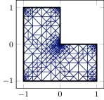
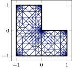
Figure 6: Adaptive triangulations on the L-shaped domain for $k=3$ from AFEM, driven by $\eta_{\rm res}(T)$ (left, $|\mathcal{T}|=882$), driven by $\eta_{\rm HHO}(T)$ (middle, $|\mathcal{T}|=907$), and driven by $\eta_{{\rm eq},0}(T)$ (right, $|\mathcal{T}|=919$).

5.6 Conclusion

The adaptive mesh-refining algorithm recovers optimal convergence rates in all three benchmarks. This holds for AFEM driven by any of the three refinement indicators derived from the GUB $\eta_{\rm res},\eta_{\rm HHO}$, and $\eta_{{\rm eq},p}$. The generated mesh sequences from the adaptive schemes, driven by the different estimators, display a very similar concentration of the local mesh-refinement as in Figure 6. All three benchmarks verify that the considered error estimators are GUB with reliability constant $1$, while the post-processing in the equilibrated GUB $\eta_{{\rm eq},p}$ produces minimal overestimation with significant additional computational costs.

Appendix Appendix A: Equilibration algorithm for higher order

The post-processed quantity $Q_{p}\in RT_{k+p}(\mathcal{T})$ from Subsection 4.2 enters the equilibrated error estimator $\eta_{{\rm eq},p}(\mathcal{T})$ in Theorem 4.1 and could be computed by a minimization problem on the vertex patches. The solution property (20) gives rise to the two cases $r=0$ if $k=0$ and $r=k+p$ if $k\geq 1$ for the polynomial degree $r$ in the equilibrium $\operatorname*{div}Q_{p}+\Pi_{r}f=0$ in $\Omega$ from (38). This appendix follows verfurth_note_2009 ; cai_robust_2012 ; bertrand_weakly_2019 ; braess_finite_2007 to compute the quantity of interest $Q_{p}-\nabla_{\rm pw}Ru_{h}$ directly in an efficient two-step procedure in 2D. Throughout this appendix, fix $k,p\in\mathbb{N}_{0}$ and abbreviate ${q}\coloneqq k+p$ and $G_{h}\coloneqq\nabla_{\rm pw}Ru_{h}\in P_{k}(\mathcal{T};\mathbb{R}^{2})$. Let the data $f\in L^{2}(\Omega)$ be given and assume, for the sake of brevity, that $f\in P_{0}(\mathcal{T})$ if $k=0$.

A.1 Overview

Recall the definition (37) of the summand $Q_{z,h}$ in $Q_{p}\coloneqq\sum_{z\in\mathcal{V}}Q_{z,h}$ from Subsection 4.2 with the piecewise Raviart-Thomas interpolation $\mathcal{I}_{\rm RT}:H^{1}(\mathcal{T};\mathbb{R}^{2})\to RT_{{q}}^{{\rm pw}}(\mathcal{T})$ (boffi_mixed_2013, , Section III.3.1). The focus is on one vertex $z\in\mathcal{V}$ with vertex-patch $\omega(z)$ and its triangulation $\mathcal{T}(z)=\{T\in\mathcal{T}\ |\ z\in T\}$. Consider set of edges $\mathcal{F}$ and the facet-spider $\mathcal{F}(z)=\{E\in\mathcal{F}\ |\ z\in E\}$ as in Figure 7. The nodal basis function $\varphi_{z}\in S^{1}(\mathcal{T}(z))$ gives rise to the discrete spaces

$$RT_{{q}}^{{\rm pw},0}(\mathcal{T}(z))\coloneqq\{\sigma_{z}\in RT_{{q}}^{\text{pw}}(\mathcal{T}(z))\ :\ \sigma_{z}\cdot\nu_{E}=0\text{ for all }E\in\mathcal{F}\setminus\mathcal{F}(z)\},$$

$$\mathcal{S}(z)\coloneqq\left\{\sigma_{z}\in RT_{{q}}^{{\rm pw},0}(z)\ :\ \begin{array}[]{llr}\operatorname*{div}\sigma_{z}&=-\Pi_{T,{{q}}}(\varphi_{z}(f+\operatorname*{div}G_{h}))&\text{ for all }T\in\mathcal{T}(z)\\ {[}\sigma_{z}\cdot\nu_{E}{]_{E}}&=-\Pi_{E,{{q}}}(\varphi_{z}[G_{h}\cdot\nu_{E}]_{E})&\text{ for all }E\in\mathcal{F}(\omega(z))\end{array}\right\}.$$

Proposition 1 (alternative minimization)

It holds

$$Q_{z,h}^{\Delta}\coloneqq Q_{z,h}-\mathcal{I}_{\rm RT}(\varphi_{z}G_{h})=\operatorname*{arg\,min}\limits_{\sigma_{z}\in\mathcal{S}(z)}\|\sigma_{z}\|_{L^{2}(\omega(z))}.$$ (64)

Proof

Recall $f_{z}=\Pi_{\tilde{p}}(\varphi_{z}f-G_{h}\cdot\nabla\varphi_{z})$ from (35). (Notice that this formula coincide with the definition (35) for $k=0$ because $f\in P_{0}(\mathcal{T})$.) Given any $\sigma_{z}\in\mathcal{S}(z)$, the commuting diagram property ${\operatorname*{div}}_{\rm pw}\circ\mathcal{I}_{\rm RT}=\Pi_{{q}}\circ{\operatorname*{div}}_{\rm pw}$ (boffi_mixed_2013, , Proposition 2.5.2) shows

$$\mathrm{div}_{\rm pw}(\sigma_{z}+\mathcal{I}_{RT}(\varphi_{z}G_{h}))=\mathrm{div}_{\rm pw}\sigma_{z}+\Pi_{\tilde{p}}\,\mathrm{div}_{\rm pw}(\varphi_{z}G_{h})=-f_{z}.$$ (65)

By design of the interpolation $\mathcal{I}_{RT}$, $(\mathcal{I}_{RT}(\varphi_{z}G_{h})_{|T}\cdot\nu_{E})_{|E}=\Pi_{E,{q}}(\varphi_{z}G_{h})_{|T}\cdot\nu_{E}$ holds and so $[\mathcal{I}_{\rm RT}(\varphi_{z}G_{h})\cdot\nu_{E}]_{E}=\Pi_{E,{{q}}}(\varphi_{z}[G_{h}\cdot\nu_{E}]_{E})$ follows for any $E\in\mathcal{F}(T)$ and $T\in\mathcal{T}$. Therefore, the jump $[\sigma_{z}+\mathcal{I}_{\rm RT}(\varphi_{z}G_{h})]_{E}\cdot\nu_{E}\equiv 0$ vanishes on $E\in\mathcal{F}(\omega(z))$, whence $\sigma_{z}+\mathcal{I}_{\rm RT}(\varphi_{z}G_{h})\in RT_{\tilde{p}}(\mathcal{T}(z))$. Since $RT_{\tilde{p}}^{{\rm pw},0}(\mathcal{T}(z))\cap H(\mathrm{div},\omega(z))=RT_{\tilde{p}}^{0}(\mathcal{T}(z))$, this and (65) imply $\sigma_{z}+\mathcal{I}_{\rm RT}(\varphi_{z}G_{h})\in\mathcal{Q}_{h}(z)$ for any $\sigma_{z}\in\mathcal{S}(z)$. In particular, $\mathcal{S}(z)+\mathcal{I}_{\rm RT}(\varphi_{z}G_{h})\subseteq\mathcal{Q}_{h}(z)$. On the other hand, similar arguments verify the reverse inclusion $\mathcal{Q}_{h}(z)\subseteq\mathcal{S}(z)+\mathcal{I}_{\rm RT}(\varphi_{z}G_{h})$. The substitution $\mathcal{S}(z)+\mathcal{I}_{\rm RT}(\varphi_{z}G_{h})=\mathcal{Q}_{h}(z)$ in (37) concludes the proof.∎

This establishes that the norm $\|Q^{\Delta}_{p}\|$ of $Q^{\Delta}_{p}\coloneqq\sum_{z\in\mathcal{V}}Q_{z,h}^{\Delta}=Q_{p}-G_{h}$ contributes to the equilibrated error estimator and the remaining parts of this appendix compute the minimizer $Q_{z,h}^{\Delta}$ of (64) in a two-step procedure.

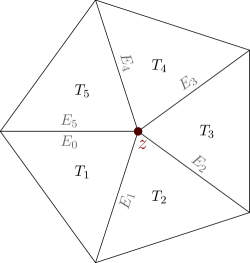
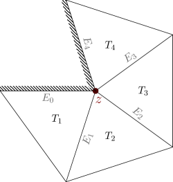
Figure 7: Triangulation $\mathcal{T}(z)$ and enumeration of the edges $\mathcal{F}(z)$ of the vertex-patch $\omega(z)$ for an internal vertex $z\in\mathcal{V}(\Omega)$ with $N=|\mathcal{T}(z)|=5$ (left) or boundary vertex $z\in\mathcal{V}(\partial\Omega)$ with $N=|\mathcal{T}(z)|=4$ (right).

First, Algorithm 2 generates the coefficients of a particular solution $\tilde{\sigma}_{z}^{\Delta}\in\mathcal{S}(z)$ in terms of the finite element basis ${\mathcal{B}}_{RT}$ of $RT_{{q}}^{{\rm pw}}(\mathcal{T}(z))$ from Subsection A.2. The second step computes the correction

$$\sigma_{z}^{\Delta}\coloneqq Q_{z,h}^{\Delta}-\tilde{\sigma}_{z}^{\Delta}=\operatorname*{arg\,min}_{\sigma_{z}\in V(z)}\|\sigma_{z}+\tilde{\sigma}_{z}^{\Delta}\|_{L^{2}(\omega(z))}$$ (66)

in terms of the low-dimensional unconstrained minimization problem over the linear space $V(z)\coloneqq\mathcal{S}(z)-\tilde{\sigma}_{z}^{\Delta}=RT_{{q}}^{{\rm pw}}(\mathcal{T}(z))\cap H(\operatorname*{div}=0,\omega(z))$ characterized in Lemma 12. Because (cai_robust_2012, , Lemma 3.1) is wrong (take, e.g., $\tau_{K}=\mathrm{curl}\,b_{K}\neq 0$ for the element bubble function $b_{K}$ in their notation to see that uniqueness for general polynomial degrees ${q}$ cannot hold) and cai_robust_2012 omits algorithmic details, this appendix focuses on the explicit characterization of the degrees of freedom for the minimization problem (66) over $V(z)$.

A.2 Degrees of freedom for $RT_{{q}}^{{\rm pw}}(T)$

This subsection introduces a basis for the Raviart-Thomas finite element on $T\in\mathcal{T}(z)$ and starts with the definition of some linear functionals on $H(\operatorname*{div},\mathcal{T})$. For any $\sigma\in H(\operatorname*{div},\mathcal{T})$, set

$$\lambda_{T,\alpha}^{\ell,m}(\sigma)\coloneqq \int_{T}\sigma\cdot e_{\alpha}\ x_{1}^{\ell}x_{2}^{m}\mathrm{dx} 0\leq\ell+m\leq{q}-1,\alpha=1,2,$$

$$\lambda_{T,\operatorname*{div}}^{\ell,m}(\sigma)\coloneqq \int_{T}\operatorname*{div}\sigma\ x_{1}^{\ell}x_{2}^{m}\mathrm{dx} 0\leq\ell+m\leq{q},$$

$$\lambda_{T,E}^{j}(\sigma)\coloneqq \int_{E}\sigma_{|T}\cdot\nu_{T}\ s^{j}\mathrm{ds} 0\leq j\leq{q},E\in\mathcal{F}(T).$$

Here and throughout, $e_{1}=(1,0)$ and $e_{2}=(0,1)$ denote the canonical unit vectors in $\mathbb{R}^{2}$. Note that the (classical) degrees of freedom for the Raviart-Thomas finite element $RT_{q}(T)$ of degree ${q}\in\mathbb{N}_{0}$ from brezzi_mixed_1991 read

$$\widetilde{\Lambda_{T}}\coloneqq\{\lambda_{T,E}^{j},\lambda_{T,\alpha}^{\ell,m}\ :\ \text{for }0\leq j\leq{q},0\leq\ell+m\leq{q}-1,\alpha=1,2,E\in\mathcal{F}(T)\}.$$

This appendix requires, for the construction of $\tilde{\sigma}_{z}^{\Delta}\in\mathcal{S}(z)$, a different set of (unisolvent) degrees of freedom $\Lambda_{T}$ for $RT_{q}(T)$ that includes the edge and divergence moments

$$\Lambda_{T}^{0}\coloneqq\{\lambda_{T,E}^{j},\lambda_{T,\operatorname*{div}}^{\ell,m}\ :\ \text{for }0\leq j\leq{q},1\leq\ell+m\leq{q},E\in\mathcal{F}(T)\}\subseteq\Lambda_{T}.$$ (67)

(The set $\Lambda_{T}^{0}$ itself is linear independent (verfurth_note_2009, , Lemma 3.1).) Given any $\Lambda_{T}$ with (67), denote the remaining $N_{q}={q}({q}-1)/2$ degrees of freedom $\Lambda_{T}\setminus\Lambda_{T}^{0}$ by $\lambda_{T}^{r}$ for $r=1,\dots,N_{q}$. Let ${\mathcal{B}}_{RT,T}=\{\varphi_{T,E}^{j},\varphi_{T,\operatorname*{div}}^{\ell,m},\varphi_{T}^{r}\}$ be the unique basis of $RT_{q}(T)$ dual to $\Lambda_{T}$ with inferred indices from $\Lambda_{T}$. Then, the collection ${\mathcal{B}}_{RT}\coloneqq\bigcup_{T\in\mathcal{T}(z)}{\mathcal{B}}_{RT,T}$ is a basis of $RT_{{q}}^{{\rm pw}}(\mathcal{T}(z))$ and any function $\sigma_{z}\in RT_{{q}}^{{\rm pw}}(\mathcal{T}(z))$ has the representation

$$\sigma_{z}\coloneqq\sum_{T\in\mathcal{T}(z)}\left(\sum_{E\in\mathcal{F}(T)}\sum_{j=0}^{q}c_{T,E}^{j}\varphi_{T,E}^{j}+\sum_{1\leq\ell+m\leq{q}}c_{T,\operatorname*{div}}^{\ell,m}\varphi_{T,\operatorname*{div}}^{\ell,m}+\sum_{r=1}^{N_{q}}c_{T}^{r}\varphi_{T}^{r}\right)$$ (68)

with coefficients $c_{T,E}^{j}=\lambda_{T,E}^{j}(\sigma_{z}),c_{T,\operatorname*{div}}^{\ell,m}=\lambda_{T,\operatorname*{div}}^{\ell,m}(\sigma_{z})$, and $c_{T}^{r}=\lambda_{T}^{r}(\sigma_{z})$ for all $T\in\mathcal{T}(z),E\in\mathcal{F}(T)$, and $0\leq j\leq{q},1\leq\ell+m\leq{q},1\leq r\leq N_{q}$. By duality, the coefficients $c_{T,E}^{j}$ with $0\leq j\leq{q}$ uniquely determine the normal trace $(\sigma_{z|T})_{|E}\cdot\nu_{E}\in P_{q}(E)$ on the edge $E\in\mathcal{F}(T)$ of $T\in\mathcal{T}(z)$. Any set of degrees of freedom $\Lambda_{T}$ with (67) works with the equilibration algorithm in A.3.

Example 3 (Construction of $\Lambda_{T}$)

This example presents a generic procedure to obtain such a set from $\widetilde{\Lambda_{T}}$. The integration by parts formula shows that the lowest-order divergence moment $\lambda_{T,{\textrm{ div }}}^{0,0}=\sum_{E\in\mathcal{F}(T)}\lambda_{T,E}^{0}$ depends linearly on the lowest-order edge moments and, similarly, the sums

$$\lambda_{T,\operatorname*{div}}^{\ell,m}+\ell\lambda_{T,1}^{\ell-1,m}+m\lambda_{T,2}^{\ell,m-1}\in(P_{\ell+m}(\mathcal{F}(T)))^{*}$$ (69)

are functionals on $P_{\ell+m}(\mathcal{F}(T))$ (summands with negative indices are understood as zero). This relation allows for the substitution of volume moments in $\widetilde{\Lambda_{T}}$ for divergence moments $\lambda_{T,\operatorname*{div}}^{\ell,m}$, $1\leq\ell+m\leq{q}$, and leads to $\Lambda_{T}$ with (67). The remaining degrees of freedom $\Lambda_{T}\setminus\Lambda_{T}^{0}$ are volume moments of the form $\lambda_{T}^{r}=\lambda_{T,\alpha}^{\ell,m}$ for a fixed $\alpha\in\{1,2\}$, e.g.,

$$\Lambda_{T}\setminus\Lambda_{T}^{0}=\{\lambda_{T,2}^{\ell,m}\ :\ 1\leq\ell\leq{q}-1,0\leq m\leq{q}-1-\ell\}.$$

A.3 Equilibration algorithm

Algorithm 2 Particular solution in $\mathcal{S}(z)$

Input: Data $f\in L^{2}(\omega(z))$ and $G_{h}\in H^{1}(\mathcal{T}(z))^{2}$ for vertex $z\in\mathcal{V}$.

1:Initialize all coefficients $c_{T,E}^{j},c_{T,\operatorname*{div}}^{\ell,m},c_{T}^{r}$ in (68) with zero.

2:for $a\coloneqq 1:N$ do

3:     $c_{T_{a},E_{a-1}}^{0}\coloneqq\begin{cases}0&\text{if }a=1,\\ ([G_{h}]_{E}\cdot\nu_{E},\varphi_{z})_{L^{2}(E_{a-1})}-c_{T_{a-1},E_{a-1}}^{0}&\text{else}\end{cases}$

4:     $c_{T_{a},E_{a\phantom{-1}}}^{0}\coloneqq(f+\operatorname*{div}G_{h},\varphi_{z})_{L^{2}(T_{a})}-c_{T_{a},E_{a-1}}^{0}$

5:     for $1\leq\ell+m\leq{q}$ do

6:         $c_{T_{a},{\textrm{ div }}}^{\ell,m}\coloneqq(f+\operatorname*{div}G_{h},\varphi_{z}x_{1}^{\ell}x_{2}^{m})_{L^{2}(T_{a})}$

7:     end for

8:     for $1\leq j\leq{q}$ do

9:         $c_{T_{a},E_{a-1}}^{j}\coloneqq 0$

10:         $c_{T_{a},E_{a\phantom{-1}}}^{j}\coloneqq([G_{h}]_{E}\cdot\nu_{E},\varphi_{z}s^{j})_{L^{2}(E_{a})}$

11:     end for

12:end for

Output: $\tilde{\sigma}_{z}^{\Delta}\in RT_{{q}}^{{\rm pw}}(\mathcal{T}(z))$ defined by (68) with coefficients $c_{T,E}^{j},c_{T,\operatorname*{div}}^{\ell,m},c_{T}^{r}$.

This subsection presents the equilibration procedure, starting with Algorithm 2, that computes an admissible function $\tilde{\sigma}_{z}^{\Delta}\in\mathcal{S}(z)$ in terms of the representation (68). Enumerate the $N\coloneqq|\mathcal{T}(z)|$ triangles $T\in\mathcal{T}(z)$ from $1$ to $N$ as in Figure 7. Any two neighbouring triangles $T_{a},T_{a+1}$ share an edge $E_{a}\coloneqq T_{a}\cap T_{a+1}$ for $a=1,...,N-1$. If $z\in\mathcal{V}(\Omega)$ is an interior vertex, $T_{1}$ and $T_{N}$ share an additional edge $E_{0}\coloneqq E_{N}\coloneqq T_{1}\cap T_{N}$. For a boundary vertex $z\in\mathcal{V}(\partial\Omega)$, $T_{1},T_{N}$ have the distinct boundary edges $E_{0},E_{N}\in\mathcal{F}(z)\cap\mathcal{F}(\partial\Omega)$. The following lemma shows correctness of Algorithm 2 under the compatibility condition (5) and represents step one of the equilibration algorithm. The final step is the local minimization problem in Lemma 12 that provides $Q_{z,h}^{\Delta}$ from (64). Both proofs are provided in A.4.

Lemma 11

Given $z\in\mathcal{V}$, let $\{\varphi_{T,E}^{j},\varphi_{T,\operatorname*{div}}^{\ell,m},\varphi_{T}^{r}\}$ be the basis of $RT_{q}(T)$ dual to $\Lambda_{T}$ with (67) for all $T\in\mathcal{T}(z)$. Suppose $f\in L^{2}(\omega(z))$ and $G_{h}\in P_{q}(\mathcal{T}(z);\mathbb{R}^{2})$ satisfy

$$(G_{h},\nabla\varphi_{z})_{L^{2}(\omega(z))}=(f,\varphi_{z})_{L^{2}(\omega(z))}\quad\text{if }z\in\mathcal{V}(\Omega).$$ (70)

Then the output of Algorithm 2 with input $f$ and $G_{h}$ defines a function $\tilde{\sigma}_{z}^{\Delta}\in\mathcal{S}(z)$.

Note that (70) is a local version of (5) and therefore holds for the HHO method with the choice $G_{h}\coloneqq\nabla_{\rm pw}Ru_{h}$ as proven in (20). This allows for the computation of $Q^{\Delta}_{p}\coloneqq\sum_{z\in\mathcal{V}}Q_{z,h}^{\Delta}=Q_{p}-G_{h}$ in terms of local and unconstrained minimization problems on the vertex-patches $\omega(z)$.

Lemma 12

Given $z\in\mathcal{V}$, let $\{\varphi_{T,E}^{j},\varphi_{T,\operatorname*{div}}^{\ell,m},\varphi_{T}^{r}\}$ be as in Lemma 11 for all $T\in\mathcal{T}(z)$ and let $\tilde{\sigma}_{z}^{\Delta}\in\mathcal{S}(z)$ be arbitrary. Then $V(z)\coloneqq\mathcal{S}(z)-\tilde{\sigma}_{z}^{\Delta}$ is a linear vector space and consists of all functions of the form

$$\sum_{a=1}^{N}\left(d_{0}(\varphi_{T_{a},E_{a-1}}^{0}-\varphi_{T_{a},E_{a}}^{0})+\sum_{\ell=1}^{q}(d_{E_{a-1}}^{\ell}\varphi_{T_{a},E_{a-1}}^{\ell}-d_{E_{a}}^{\ell}\varphi_{T_{a},F_{a}}^{\ell})+\sum_{r=1}^{N_{q}}d_{T_{a}}^{r}\varphi_{T_{a}}^{r}\right)$$ (71)

for arbitrary $d_{0},d_{E_{a}}^{\ell},d_{T_{a}}^{r}\in\mathbb{R}$ with $\ell=1,...,{q},r=1,...,N_{q},a=1,...,N$ (and $d_{E_{0}}^{\ell}=d_{E_{N}}^{\ell}$ for $z\in\mathcal{V}(\Omega)$) and the enumeration of $\mathcal{T}(z)$ as in Figure 7. Furthermore, $Q_{z,h}^{\Delta}=\tilde{\sigma}_{z}^{\Delta}+\sigma_{z}^{\Delta}$ holds for the solution $\sigma_{z}^{\Delta}\in V(z)$ to the $1+{q}|\mathcal{F}(z)|+{q}({q}-1)/2N$-dimensional minimization problem (66).

A.4 Proofs

The remaining parts of this appendix are devoted to the verification of Lemmas 11–12.

Proof (of Lemma 11)

Enumerate $\mathcal{T}(z)$ as in A.3 and recall the definition of the jump $[G_{h}]_{E}=G_{h}|_{T_{+}}-G_{h}|_{T_{-}}$ on the interior edge $E=T_{+}\cap T_{-}$ shared by $T_{+},T_{-}\in\mathcal{T}$, and $[G_{h}]_{E}=G_{h}|_{T_{+}}$ for the unique triangle $T_{+}\in\mathcal{T}$ with $E\subset T_{+}$ for the boundary edge $E\in\mathcal{F}(\partial\Omega)$. First, observe that $\sigma_{z}\in RT_{{q}}^{{\rm pw}}(\mathcal{T}(z))$ lies in $RT_{{q}}^{{\rm pw},0}(\mathcal{T}(z))$ if and only if the coefficients $c_{T,E}^{j}=0$ in the representation (68) are zero for $0\leq j\leq{q}$ at the edge $E\in\mathcal{F}(T)\setminus\mathcal{F}(z)$ in $T\in\mathcal{T}$ opposing $z$. By definition, $\sigma_{z}\in RT_{{q}}^{{\rm pw},0}(\mathcal{T}(z))$ belongs to $\mathcal{S}(z)$ if and only if

$$\lambda_{T,\operatorname*{div}}^{\ell,m}(\sigma_{z}) =(f+\operatorname*{div}G_{h},\varphi_{z}x_{1}^{\ell}x_{2}^{m})_{L^{2}(T)} \text{for all }0\leq\ell+m\leq{q},T\in\mathcal{T}(z),$$ (72)

$$(\lambda_{T_{+},E}^{j}+\lambda_{T_{-},E}^{j})(\sigma_{z}) =([G_{h}]_{E}\cdot\nu_{E},\varphi_{z}s^{j})_{L^{2}(E)} \text{for all }0\leq j\leq{q},E\in\mathcal{F}(\omega(z)).$$ (73)

This translates into equivalent conditions on the coefficients of $\sigma_{z}$ in the representation (68), namely, for all $a=1,...,N$,

$$c_{T_{a},E_{a}}^{0} =(f+\operatorname*{div}G_{h},\varphi_{z})_{L^{2}(T_{a})}-c_{T_{a},E_{a-1}}^{0},$$ (74)

$$c_{T_{a},\operatorname*{div}}^{\ell,m} =(f+\operatorname*{div}G_{h},\varphi_{z}x_{1}^{\ell}x_{2}^{m})_{L^{2}(T_{a})} \text{for all }1\leq\ell+m\leq{q},$$ (75)

$$c_{T_{a},E_{a-1}}^{j} =d_{E_{a-1}}^{j} \text{for all }0\leq j\leq{q},$$ (76)

$$c_{T_{a},E_{a}}^{j} =([G_{h}]_{E}\cdot\nu_{E},\varphi_{z}s^{j})_{L^{2}(E_{a})}-d_{E_{a}}^{j} \text{for all }0\leq j\leq{q},$$ (77)

where $d_{E_{a}}^{\ell}\in\mathbb{R}$. Since $\sigma_{z}\in RT_{{q}}^{{\rm pw},0}(\mathcal{T}(z))$ vanishes at the other edges $E\in\mathcal{F}\setminus\mathcal{F}(z)$, $\lambda_{T_{a},\operatorname*{div}}^{0,0}(\sigma_{z})=c_{T_{a},E_{a-1}}^{0}+c_{T_{a},E_{a}}^{0}$ and (74)–(75) are equivalent to (72). The identification $d_{E_{0}}^{\ell}=d_{E_{N}}^{\ell}$ for an interior vertex $z\in\mathcal{V}(\Omega)$ with $E_{0}=E_{N}\in\mathcal{F}(z)$ shows that (76)–(77) are equivalent to (73). This identification is well defined. Note that, whereas there is no condition on $d_{E_{a}}^{\ell}$ for $1\leq\ell\leq{q}$, the combination of (74) and (76) with (77) shows the implicit extra condition

$$d_{E_{a}}^{0}=d_{E_{0}}^{0}+\sum_{\alpha=1}^{a}\left(([G_{h}]_{E}\cdot\nu_{E},\varphi_{z})_{L^{2}(E_{\alpha})}-(f+\operatorname*{div}G_{h},\varphi_{z})_{L^{2}(T_{\alpha})}\right)\quad\text{for }a=0,...,N.$$

For an interior vertex $z\in\mathcal{V}(\Omega)$, an integration by parts and (70) show that the sum on the right-hand side above vanishes for $a=N$, whence $d_{E_{N}}^{0}=d_{E_{0}}^{0}$ is indeed well defined. Furthermore, there is no condition on the coefficients $c_{T_{a}}^{r}$ for all $T_{a}\in\mathcal{T}(z)$ and $r=1,...,N_{q}$ and $c_{T_{a}}^{r}=d_{T_{a}}^{r}$ is a further degree of freedom.

Algorithm 2 finds coefficients that satisfy (74)–(77) in a loop over $a=1,...,N$ and therefore defines $\tilde{\sigma}_{z}^{\Delta}\in\mathcal{S}(z)$ by (68).∎

Proof (of Lemma 12)

This follows immediately after revisiting the proof of Lemma 11 for an arbitrary function $\sigma_{z}\in RT_{{q}}^{{\rm pw},0}(\mathcal{T}(z))$. Since $\sigma_{z}\in\mathcal{S}(z)$ is equivalent to (74)–(77) for the representation (68) of $\sigma_{z}$ in the given basis, all functions $\sigma_{z}\in\mathcal{S}(z)-\tilde{\sigma}_{z}^{\Delta}$ are of the form (71) for arbitrary $d_{0},d_{E_{a}}^{\ell},d_{T_{a}}^{r}\in\mathbb{R}$ with $\ell=1,...,{q}$, $r=1,...,N_{q}$, and $a=1,...,N$ (and $d_{E_{0}}^{\ell}=d_{E_{N}}^{\ell}$ for $z\in\mathcal{V}(\Omega)$). Hence, the dimension of the linear space $V(z)=\mathcal{S}(z)-\tilde{\sigma}_{z}^{\Delta}$ is $1+{q}|\mathcal{F}(z)|+{q}({q}-1)/2N$. The claim follows from Proposition 1 by observing

$$Q_{z,h}^{\Delta}\coloneqq \operatorname*{arg\,min}\limits_{\sigma_{z}\in\mathcal{S}(z)}\|\sigma_{z}\|_{L^{2}(\omega(z))}=\tilde{\sigma}_{z}^{\Delta}+\operatorname*{arg\,min}\limits_{\sigma_{z}\in\mathcal{S}(z)-\tilde{\sigma}_{z}^{\Delta}}\|\tilde{\sigma}_{z}^{\Delta}+\sigma_{z}\|_{L^{2}(\omega(z))}.\quad\qed$$

References

• (1) Ainsworth, M.: Robust a posteriori error estimation for nonconforming finite element approximation. SIAM J. Numer. Anal. 42(6), 2320–2341 (2005)
• (2) Ainsworth, M.: A posteriori error estimation for lowest order Raviart-Thomas mixed finite elements. SIAM J. Sci. Comput. 30, 189–204 (2007)
• (3) Ainsworth, M., Oden, J.T.: A unified approach to a posteriori error estimation using element residual methods. Numer. Math. 65, 23–50 (1993)
• (4) Alonso, A.: Error estimators for a mixed method. Numer. Math. 74(4), 385–395 (1996)
• (5) Bertrand, F., Boffi, D.: The Prager-Synge theorem in reconstruction based a posteriori error estimation. In: 75 years of mathematics of computation, vol. 754, pp. 45–67. Amer. Math. Soc., [Providence], RI (2020)
• (6) Bertrand, F., Kober, B., Moldenhauer, M., Starke, G.: Weakly symmetric stress equilibration and a posteriori error estimation for linear elasticity. Numer. Methods Partial Differential Equations 37(4), 2783–2802 (2021)
• (7) Boffi, D., Brezzi, F., Fortin, M.: Mixed finite element methods and applications, vol. 44. Springer, Heidelberg (2013)
• (8) Bonito, A., Nochetto, R.H.: Quasi-optimal convergence rate of an adaptive discontinuous Galerkin method. SIAM J. Numer. Anal. 48(2), 734–771 (2010)
• (9) Braess, D.: Finite Elements: theory, fast solvers, and applications in Solid Mechanics, third edn. Cambridge University Press, Cambridge (2007)
• (10) Braess, D., Pillwein, V., Schöberl, J.: Equilibrated residual error estimates are $p$-robust. Comput. Methods Appl. Mech. Engrg. 198, 1189–1197 (2009)
• (11) Brezzi, F., Fortin, M.: Mixed and hybrid finite element methods, vol. 15. Springer, New York (1991)
• (12) Cai, Z., Zhang, S.: Robust equilibrated residual error estimator for diffusion problems: conforming elements. SIAM J. Numer. Anal. 50(1), 151–170 (2012)
• (13) Carstensen, C.: A posteriori error estimate for the mixed finite element method. Math. Comp. 66(218), 465–476 (1997)
• (14) Carstensen, C.: A unifying theory of a posteriori finite element error control. Numer. Math. 100(4), 617–637 (2005)
• (15) Carstensen, C., Ern, A., Puttkammer, S.: Guaranteed lower bounds on eigenvalues of elliptic operators with a hybrid high-order method. Numer. Math. 149(2), 273–304 (2021)
• (16) Carstensen, C., Feischl, M., Page, M., Praetorius, D.: Axioms of adaptivity. Comput. Math. Appl. 67(6), 1195–1253 (2014)
• (17) Carstensen, C., Gedicke, J., Rim, D.: Explicit error estimates for Courant, Crouzeix-Raviart and Raviart-Thomas finite element methods. J. Comput. Math. 30(4), 337–353 (2012)
• (18) Carstensen, C., Gudi, T., Jensen, M.: A unifying theory of a posteriori error control for discontinuous Galerkin FEM. Numer. Math. 112(3), 363–379 (2009)
• (19) Carstensen, C., Hellwig, F.: Constants in discrete Poincaré and Friedrichs inequalities and discrete quasi-interpolation. Comput. Methods Appl. Math. 18(3), 433–450 (2018)
• (20) Carstensen, C., Hu, J.: A unifying theory of a posteriori error control for nonconforming finite element methods. Numer. Math. 107(3), 473–502 (2007)
• (21) Carstensen, C., Peterseim, D., Schröder, A.: The norm of a discretized gradient in $H(\mathrm{div})^{*}$ for a posteriori finite element error analysis. Numer. Math. 132, 519–539 (2016)
• (22) Carstensen, C., Rabus, H.: Axioms of adaptivity with separate marking for data resolution. SIAM J. Numer. Anal. 55(6), 2644–2665 (2017)
• (23) Ciarlet, P., Dunkl, C.F., Sauter, S.A.: A family of Crouzeix-Raviart finite elements in 3D. Anal. Appl. (Singap.) 16(5), 649–691 (2018)
• (24) Dauge, M.: Elliptic boundary value problems on corner domains, vol. 1341. Springer-Verlag, Berlin (1988)
• (25) Di Pietro, D.A., Droniou, J.: The hybrid high-order method for polytopal meshes, vol. 19. Springer, Cham (2020)
• (26) Di Pietro, D.A., Ern, A.: A hybrid high-order locking-free method for linear elasticity on general meshes. Comput. Methods Appl. Mech. Engrg. 283, 1–21 (2015)
• (27) Di Pietro, D.A., Ern, A., Lemaire, S.: An arbitrary-order and compact-stencil discretization of diffusion on general meshes based on local reconstruction operators. Comput. Methods Appl. Math. 14(4), 461–472 (2014)
• (28) Ern, A., Guermond, J.L.: Finite elements I—Approximation and interpolation, vol. 72. Springer, Cham (2021)
• (29) Ern, A., Guermond, J.L.: Finite elements II—Galerkin approximation, elliptic and mixed PDEs, vol. 73. Springer, Cham (2021)
• (30) Ern, A., Vohralík, M.: Polynomial-degree-robust a posteriori estimates in a unified setting for conforming, nonconforming, discontinuous Galerkin, and mixed discretizations. SIAM J. Numer. Anal. 53(2), 1058–1081 (2015)
• (31) Ern, A., Vohralík, M.: Stable broken $H^{1}$ and $H({\rm div})$ polynomial extensions for polynomial-degree-robust potential and flux reconstruction in three space dimensions. Math. Comp. 89(322), 551–594 (2020)
• (32) Ern, A., Zanotti, P.: A quasi-optimal variant of the hybrid high-order method for elliptic partial differential equations with $H^{-1}$ loads. IMA J. Numer. Anal. 40(4), 2163–2188 (2020)
• (33) Girault, V., Raviart, P.A.: Finite element methods for Navier-Stokes equations, vol. 5. Springer, New York (1986)
• (34) Kikuchi, F., Liu, X.: Estimation of interpolation error constants for the $P_{0}$ and $P_{1}$ triangular finite elements. Comput. Methods Appl. Mech. Engrg. 196(37-40), 3750–3758 (2007)
• (35) Oikawa, I.: A hybridized discontinuous Galerkin method with reduced stabilization. J. Sci. Comput. 65(1), 327–340 (2015)
• (36) da Veiga, L.B., Canuto, C., Nochetto, R.H., Vacca, G., Verani, M.: Adaptive VEM: Stabilization-free a posteriori error analysis (2021)
• (37) Verfürth, R.: A note on constant-free a posteriori error estimates. SIAM J. Numer. Anal. 47(4), 3180–3194 (2009)
• (38) Verfürth, R.: A posteriori error estimation techniques for finite element methods. Oxford University Press, Oxford (2013)
• (39) Wang, J., Ye, X.: A weak Galerkin finite element method for second-order elliptic problems. J. Comput. Appl. Math. 241, 103–115 (2013)