Interacting Dirac fermions and the rise of Pfaffians in graphene

Abstract

Fractional Quantum Hall effect (FQHE) is a unique many-body phenomenon, which was discovered in a two-dimensional electron system placed in a strong perpendicular magnetic field. It is entirely due to the electron-electron interactions within a given Landau level. For special filling factors of the Landau level, a many-particle incompressible state with a finite collective gap is formed. Among these states, when the Landau level is half filled, there is a special FQHE state that is described by the Pfaffian function and the state supports charged excitations that obey non-Abelian statistics. Such a $1/2$-FQHE state can be realized only for a special profile of the electron-electron potential. For example, for conventional electron systems the $1/2$-FQHE state occurs only in the second Landau level, while in a graphene monolayer, no $1/2$-FQHE state can be found in the first and the second Landau levels. Another type of low-dimensional system is the bilayer graphene, which consists of two graphene monolayers coupled through the inter-layer hopping. The system is quasi-two-dimensional, which makes it possible to tune the inter-electron interaction potential by applying either the bias voltage or the magnetic field that is applied parallel to the bilayer. Interestingly, in the bilayer graphene with AB staking, there is one Landau level per valley where the $1/2$-FQHE state can indeed be present. The properties of that $1/2$-FQHE state have a nonmonotonic dependence on the applied magnetic field and this state can be even more stable than the one discovered in conventional electron systems.

Key points

• In two-dimensional electron systems an externally applied magnetic field results in the formation of highly discrete and degenerate Landau levels.

• In a strong enough magnetic field, the discrete nature of the energy spectrum of two-dimensional electrons results in the Integer Quantum Hall effect, which happens when integer number of Landau levels are occupied.

• For a partially filled Landau levels, inter-electron interactions result in formation of incompressible liquids, which manifest themselves as the Fractional Quantum Hall Effect.

• The conventional FQHE corresponds to filling factors of type $p/q$, where $q$ is odd.

• The unconventional FQHE at half-filling ($\nu=1/2$) of a given Landau level is described by the Pfaffian function as the wave function of the ground state and has excitations with the charge of $e/4$ and obey non-abelian statistics.

• For conventional 2D systems, $1/2$-FQHE is realized only in the $n=1$ Landau level.

• For graphene monolayer, there is no $\nu=1/2$ incompressible liquid in any Landau level.

• For bilayer graphene there is a special Landau level in which the stability of the $\nu=1/2$ incompressible state can be tuned by the magnitude and direction of the magnetic field and the bias voltage.

I Introduction

A moving charge placed in an external magnetic field experiences a magnetic force, which can change only the direction of the charge velocity but not its magnitude. One of the manifestations of this property of the magnetic field is the Hall effect. The Hall effect occurs when the current flows through a solid and the magnetic field is applied perpendicular to the current. In this case the voltage difference, which is called the Hall voltage, is generated across the conductor in the direction transverse to both the current and the magnetic field. This effect was discovered by Edwin Hall in 1879 Hall (1879). If the electric current is in the $x$ direction with the current density of $j_{x}$ and magnetic field is in the $z$ direction, then there is a Hall electric field generated in the $y$ direction. The strength of the Hall effect is characterized by the Hall coefficient defined by the following expression Ashcroft and Mermin (1976); Hurd (1972); Kittel (2005)

$$R_{H}=\frac{E_{y}}{j_{x}B_{z}}.$$ (1)

It is possible to show that, within the classical approach, the Hall constant is related to the charge of the carriers, $q$, and their density, $n$,

$$R_{H}=\frac{1}{nq}.$$ (2)

One important property of this expression is that the Hall constant and correspondingly the Hall voltage depends on the sign of carrier’s charge, $q$. For example, for semiconductors, when the carriers are negatively charged electrons or positively charged holes, the Hall constant can be negative or positive depending on the type of the major carriers.

The above expression for the Hall coefficient corresponds to the classical description of the electron dynamics in a magnetic field, or in the low magnetic field limit. With increasing magnetic field, the electron dynamics in the magnetic field becomes essentially quantum mechanical, which results in quantization of the corresponding energy spectrum and formation of highly degenerate and discrete Landau levels Landau and Lifshitz (1965). The energy distance between the Landau levels is proportional to the magnetic field. Due to discrete nature of the energy spectrum of carriers, the diagonal resistance of a solid as a function of the magnetic field shows oscillations, which are called the Shubnikov de Haas oscillations Seiler and Stephens (1991).

More interesting and unexpected phenomena occur in two-dimensional (2D) electron systems, such as in heterojuctions, atomic monolayers, or in quantum wells. If the magnetic field is applied perpendicular to the 2D layer, i.e., the $(x,y)$ plane, then for weak magnetic fields there is the classical Hall effect, which can be also characterized by the Hall resistance $R_{xy}$

$$R_{xy}=\frac{E_{y}}{j_{x}}=R_{H}B_{z}.$$ (3)

Therefore in the classical regime, i.e., in a weak magnetic field, the Hall resistance is proportional to the magnetic field, $B_{z}$. At the same time, in stronger magnetic fields when the quantization of the in-plane electron dynamics results in Landau levels, there is another unique effect, which is the Integer Quantum Hall Effect (IQHE) Stone (1992); Klitzing et al. (1980); Yoshioka (2002); Prange and Girvin (1987); Chakraborty and Pietiläinen (1995); Klitzing (2017); von Klitzing et al. (2020). In this regime, the Hall resistance takes only quantized values of the form

$$R_{xy}=\frac{h}{e^{2}\nu},$$ (4)

where $h$ is the Plank constant, $e$ is the electron charge, and $\nu$ is an integer, $\nu=1,2,3,\ldots$. The integer number $\nu$ corresponds to the number of completely filled Landau levels and whenever the Fermi energy is between the two Landau levels $n$ and $n+1$, the Hall resistance is constant, while the longitudinal resistance, $R_{xx}$, becomes zero. Strictly speaking, to understand the Quantum Hall Effect we also need to consider broadening of the Landau levels due to disorder and spatial localization of the in-gap electron states between the Landau levels Stone (1992); Chakraborty and Pietiläinen (1995). However the main condition for the IQHE is the existence of the gaps in the energy spectrum which naturally occurs in 2D systems in a strong magnetic field.

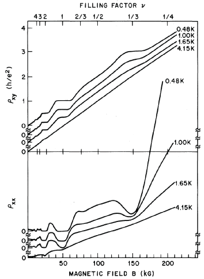
Figure 1: Non-diagonal and diagonal resistivities, $\rho_{xy}$ and $\rho_{xx}$, as a function of magnetic field, $B$. The sample is GaAs-Al_0.3Ga${}_{0}.7$As with electron density of $n=1.23\times 10^{11}$ cm^-2 and mobility $\mu=90000$ cm²/Vs (Adapted from Tsui et al. (1982)).

The IQHE was discovered experimentally in 1980 and two years later another unexpected (and more spectacular) effect was observed in even stronger magnetic fields, and in better quality samples. This effect is known as the Fractional Quantum Hall Effect (FQHE) Tsui et al. (1982); Chakraborty and Pietiläinen (1995). In this case the filling factor $\nu$ in Eq. (4) is fractional and corresponds to partial occupation of a given Landau level. Since all levels within the Landau level are degenerate, the electron-electron interaction completely determines the properties of the system. At special fractional occupations of the Landau level, the interaction generates the incompressible ground states with gapped excitations, which finally results in the FQHE. The primary filling factors where the FQHE occur are $\nu=\frac{1}{3},\frac{2}{3},\frac{1}{5},\frac{2}{5},\frac{3}{5},\frac{1}{7}$ etc. Prange and Girvin (1987); Chakraborty and Pietiläinen (1995); Halperin and Jain (2020). In all these cases the denominator is an odd number, which is due to the fermionic nature of electrons.

II Fractional Quantum Hall Effect

First, we consider the conventional two-dimensional electron systems, such as the ones grown in heterojuncions or in a quantum well, for which the low-energy dispersion relation is parabolic. The Hamiltonian of such systems has the following form

$${\cal H}_{c}=\frac{\vec{p}^{2}}{2m^{*}},$$ (5)

where $\vec{p}$ is the two-dimensional momentum and $m^{*}$ is the electron effective mass. When the system is placed in a perpendicular external magnetic field, the Hamiltonian becomes

$${\cal H}_{c}=\frac{\mathbf{\pi}^{2}}{2m^{*}},$$ (6)

where $\vec{\pi}=\vec{p}+e\vec{A}/c$ is the generalized momentum and $\vec{A}$ is the vector potential. The energy spectrum of the Hamiltonian (6) consists of highly degenerate discrete Landau levels Landau and Lifshitz (1965) with energy

$$\epsilon_{n}=\hbar\omega_{B}\left(n+\frac{1}{2}\right),$$ (7)

where $\omega_{B}=eB/m^{*}$ is the cyclotron frequency and $n=0,1,2,\ldots$ is the Landau level index. We write the corresponding Landau eigenfunctions as $\phi_{n,m}$, where the index $m$ labels the degenerate wavefunctions within a given Landau level and is determined by the choice of the gauge. For example, in the Landau gauge, $A_{x}=0$ and $A_{y}=Bx$, the index $m$ is the $y$-component of the momentum, while in the symmetric gauge, $\vec{A}=\frac{1}{2}\vec{B}\times\vec{r}$, the index $m$ is the $z$-component of electron angular momentum Landau and Lifshitz (1965). In what follows, we consider $m$ as the $z$ component of the angular momentum.

When a given Landau level is partially occupied by electrons, the properties of the system is completely determined by the electron-electron interactions. If the mixing of Landau levels due to the interactions is weak, then the interaction properties of electrons within a single Landau level are completely determined by the Haldane pseudopotentials $V^{(n)}_{m}$ Haldane (1983). The Haldane pseudopotential $V^{(n)}_{m}$ is the energy of two electrons with the relative angular momentum $m$ and they can be found from the following expression Haldane (1987)

$$V_{m}^{(n)}=\int_{0}^{\infty}\frac{dq}{2\pi}qV(q)\left[F_{n}(q)\right]^{2}L_{m}(q^{2}){\rm e}^{-q^{2}},$$ (8)

where $L_{m}(x)$ are the Laguerre polynomials, $V(q)=2\pi{\rm e}^{2}/(\kappa\ell_{0}q)$ is the Coulomb interaction in the momentum space, $\kappa$ is the dielectric constant, and $F_{n}(q)$ is the form factor of the $n$-th Landau level. The form factor is totally determined by the structure of the wavefunctions of the corresponding Landau level. Different two-dimensional systems, such as graphene monolayer, transition-metal dichalcogenide monolayer, graphene bilayer, etc., have different form factors $F_{n}(q)$, but in all cases, the corresponding Haldane pseudopotentials are given by the same expression (8). For conventional two-dimensional electron systems with Landau wavefunctions $\phi_{n,m}$ the form factor is Haldane (1987)

$$F_{n}(q)=L_{n}\left(q^{2}/2\right).$$ (9)

If the electron system is fully spin polarized then the spatial component of the many-particle wavefunction is antisymmetric with respect to the particle exchange. In this case, only the Haldane pseudopotentials, $V_{m}^{(n)}$, with odd values of $m$, $m=1,3,5,\ldots$, determine the properties of the system. The nature of the ground state mainly depends on the ratio of the first few pseudopotentials, $V_{1}^{(n)}/V_{3}^{(n)}$ and $V_{3}^{(n)}/V_{5}^{(n)}$.

At special values of the filling factor $\nu$, which is defined as $\nu=N_{e}/N_{0}$, where $N_{e}$ is the number of electrons in a given Landau level and $N_{0}$ is its degeneracy, the electron system becomes incompressible with a finite excitation gap. This incompressibility is entirely due to electron-electron interactions and is determined by the values of the Haldane pseudopotentials. Only for these filling factors the FQHE can be observed.

The conventional FQHE occurs at the filling factors of the form $p/q$, where $q$ is odd, which is related to the antisymmetric property of a many-particle electron wavefunction when two particles are interchanged, i.e., $\Psi(\vec{r}_{1},\vec{r}_{2},\vec{r}_{3},\ldots)=-\Psi(\vec{r}_{2},\vec{r}_{1},\vec{r}_{3},\ldots)$. A prominent example of this type of FQHE is the $1/q$ sequence, i.e., $1/3$, $1/5$ etc. The corresponding many-particle wave function is well described by the Laughlin function Laughlin (1983) of the form

$$\Psi(z_{1},z_{2},z_{3},\ldots)=\prod_{i<j}(z_{i}-z_{j})^{q}\exp\left(-\sum_{i}\frac{z_{i}^{2}}{4\ell_{0}^{2}}\right),$$ (10)

where the positions of electrons are described in terms of complex variable $z=x-iy$. The Laughlin function (10) corresponds to the filling factor $1/q$ and is very close to the exact many-particle wave function of the system. The accuracy of the trial wave functions, for instance the Laughlin functions is tested through numerical calculations for a finite-size electron system. For a finite-size system placed in an external magnetic field, the many-particle basis is finite, which allows us to find both the ground state and the excitation spectrum of the system. Then, the overlap of the trial function with the exact ground state wave function of the many-particle system can be determined and that can be used to test the accuracy of the trial approximation. The incompressibility of the system is determined by the magnitude of the gap in the collective excitations of the system. Another interesting property of the $1/q$ FQHE, which is described by the Laughlin function, is that the charged excitations have fractional charge $e^{*}=e/q$. For example, for the $1/3$-FQHE the quasiparticles carry a fractional charge $e^{*}=e/3$.

Our fundamental understanding of the origin of the odd-denominator FQHE is from the brilliant work of Laughlin which requires that we consider a incompressible fluid that has no long-range positional order. The incompressibility implies that all the excited states have a non-zero energy difference from the ground state. The ground state can be fully spin polarized or also have spin degree of freedom Chakraborty and Zhang (1984); Chakraborty et al. (1986); Apalkov et al. (2001) in the ground state and spin-reversed excitations. It is worth emphasizing that despite the torrent of ideas unleased by the Laughlin function, the origin of incompressibility in the Laughlin state still remains unresolved Haldane (2011).

In addition to the conventional FQHE set of type $p/q$, where $q$ is odd, another type of FQHE corresponding to the filling $5/2$ has been discovered experimentally (Willett et al., 1987; Willett, 2013). This filling factor implies that there are two completely occupied Landau levels, which correspond to spin-up and spin-down Landau levels with index $n=0$, and the next Landau level is half-filled. It means that in the $n=1$ Landau level the $1/2$-FQHE occurs, i.e., the filling factor of the $n=1$ Landau level is $\nu=1/2$. This unusual FQHE cannot be described by the Laughlin function (10). This is because the many-particle wave function should be antisymmetric with respect to the particle interchange, because the corresponding electrons are fermions and $q$ must be an odd integer. But for $q=2$, the Laughlin function is symmetric, and therefore describes a system of bosons. Another important property of the $1/2$-FQHE is that the $1/2$ incompressible liquid is realized only in higher Landau levels, for example, for $n=1$ but not for the $n=0$ level. Different wavefunctions have been proposed theoretically to describe this state. Among them are the Pfaffian Moore and Read (1991), anti-Pfaffian Levin et al. (2007), particle-hole symmetric Pfaffian Son (2015), and the 221-parton Wen (1991) wavefunctions. The $1/2$-FQHE is also sensitive to the inter-Landau mixing Rezayi (2017) which modifies the electron-electron interaction potential Peterson and Nayak (2013) and opens up the possibility to observe the $1/2$-FQHE in higher Landau levels Kim et al. (2019) where the inter-Landau mixing becomes strong. Below we consider the properties of the $1/2$-FQHE, which is described only by the Pfaffian wavefunction.

II.1 Pfaffian function

Some properties of the FQHE states can be understood by looking at the specially created composite objects, that are called the composite fermions. The composite fermion is an electron with an even number of flux quanta attached to it. These objects still have the same Fermi statistics as original electrons, but they feel a different magnetic field. To understand their properties, first, let us consider a fully filled Landau level. In this case, there is one magnetic flux quantum per each electron and under this condition we have the IQHE. Now let us consider a Landau level with the filling factor of $\nu=1/3$, i.e., only $1/3$ states within a given Landau level are occupied. For such a system, there are three magnetic flux quanta per electron and this state corresponds to the $\nu=1/3$-FQHE. The composite fermions for this system are electrons bound to two magnetic flux quanta each. Therefore, for these composite fermions (one electron plus two flux quanta), there is one magnetic flux quanta per fermion, which corresponds to a fully occupied Landau level and is therefore, the IQHE of composite fermions. Another way to state this is that, the FQHE for electrons is the IQHE for composite fermions. This correspondence exists only for the FQHE of type of $p/q$, where $q$ is odd. As an example, for $\nu=1/5$ the composite fermion is an electron plus four magnetic flux quanta and the composite fermions all occupy the first Landau level. It is important that the number of magnetic flux quanta attached to an electron is even. Only in this case the composite particles have the same Fermi statistics as electrons.

A unique situation occurs for the Landau level that is exactly half filled. For such a system, the composite fermion picture dictates that there are two magnetic flux quanta associated with each electron. In that case, a composite fermion comprise of an electron bound to two magnetic flux quanta and in a mean-field picture, the system of composite fermions does not experience a net magnetic field Halperin et al. (1993). The properties of this composite fermion system are determined by the inter-fermion interaction, i.e., by the Haldane pseudopotentials. For the $n=0$ Landau level, the composite fermions forms a gapless composite Fermi liquid. A more interesting situation happens for the $n=1$ Landau level, i.e., for the total filling factor $\nu=5/2$. In this case, the theoretical and experimental results suggest that the system forms a gapped state which is due to pairing of the composite fermions, i.e., by formation of Cooper pairs, similar to what we see in the supercoductor systems. The pairing symmetry can then be different and below we consider only one type of symmetry, i.e., when the Cooper pairs of composite fermions have angular momentum $-1$. It was proposed that the corresponding ground state of the system expressed in terms of the coordinates of original electrons is described by the Pfaffian Moore and Read (1991); Greiter et al. (1991, 1992); Nayak et al. (2008) function, which has the following form

$$\Psi_{\mbox{Pf}}=\mbox{Pf}\left[\frac{1}{z_{i}-z_{j}}\right]\prod_{i<j}(z_{i}-z_{j})^{2}\exp\left(-\sum_{i}\frac{z_{i}^{2}}{4\ell_{0}^{2}}\right),$$ (11)

where the Pfaffian is defined as Moore and Read (1991); Greiter (2011)

$${\rm Pf}\,\left[\mathbf{M}\right]=\frac{1}{2^{N/2}\left(N/2\right)!}\sum_{\sigma\in S_{N}}{\rm sgn}\,\sigma\prod_{l=1}^{N/2}M_{\sigma(2l-1)\sigma(2l)},$$ (12)

for an $N\times N$ antisymmetric matrix $\mathbf{M}$ whose elements are $M_{ij}$, where $N$ is an even number. Here $S_{N}$ is the group of permutations of $N$ objects.

Historically, the concept of Pfaffians arose from a very surprising mathematical result: Consider the determinant of a $N\times N$ antisymmetric matrix $\mathbf{M}=[M_{ij}]$ written as $\det[M_{ij}]_{1\leq i,j\leq N}$ in which $M_{ij}=-M_{ji}$ for $i,j=1,2,\ldots,N$. If $\mathbf{M}=-\mathbf{M}^{T}$ is an antisymmetric matrix of order $N$ then $\det[\mathbf{M}]=(-1)^{N}\det[\mathbf{M}]$ so that if the order is odd, then the determinant vanishes. However, when $N=2m$, then the determinant is the square of a polynomial in coefficients of the given determinant. This result was first discovered by the British mathematician Arthur Cayley in 1847 Cayley (1847); Halton (1966), who named this polynomial Pfaffian in honor of the great German mathematician Johann Pfaff, who discovered it in 1815, in the course of his work on differential equations.

For $N=2$,

$$\det\left|\begin{array}[]{cc}0&M_{12}\\ -M_{12}&0\end{array}\right|=\left(M_{12}\right)^{2},$$ (13)

and the Pfaffian is ${\rm Pf}\left[\mathbf{M}\right]=M_{12}$. Similarly, for $N=4$,

$$\det\left|\begin{array}[]{cccc}0&M_{12}&M_{13}&M_{14}\\ -M_{12}&0&M_{23}&M_{24}\\ -M_{13}&-M_{23}&0&M_{34}\\ -M_{14}&-M_{24}&-M_{34}&0\end{array}\right|=\left(M_{12}M_{34}-M_{13}M_{24}+M_{14}M_{23}\right)^{2},$$ (14)

and the corresponding Pfaffian is

$${\rm Pf}\,\left[\mathbf{M}\right]=M_{12}M_{34}-M_{13}M_{24}+M_{14}M_{23}.$$ (15)

There are three terms in the above expression. For a general antisymmetric matrix $N\times N$, the number of terms in the pfaffian is $(N-1)!!$. The Pfaffians are sometimes referred to as triangular determinant or half-determinant Crilly (2016),

$${\rm Pf}\,\left[\mathbf{M}\right]=\left.\begin{array}[]{cccc}|M_{12}&M_{13}&M_{14}\\ &M_{23}&M_{24}\\ &&M_{34}\end{array}\right|.$$ (16)

Moving on, one can obtain the following relation between the determinant of the matrix $\mathbf{M}$ and its Pfaffian Cayley (1847); Halton (1966),

$$\rm{det}\left[\mathbf{M}\right]=\left({\rm Pf}\,\left[\mathbf{M}\right]\right)^{2}.$$ (17)

This relation can be generalized for a special partially antisymmetric matrix of the form Cayley (1847); Bajdich et al. (2008)

$$\mathrm{det}\left[\begin{array}[]{ccccc}0&b_{12}&b_{13}&\ldots&b_{1N}\\ -a_{12}&0&a_{23}&\ldots&a_{2N}\\ -a_{13}&-a_{23}&0&\ldots&a_{3N}\\ \vdots&\vdots&\vdots&\vdots&\vdots\\ -a_{1N}&-a_{2N}&-a_{3N}&\ldots&0\end{array}\right]=\mathrm{Pf}\left[\begin{array}[]{ccccc}0&a_{12}&a_{13}&\ldots&a_{1N}\\ -a_{12}&0&a_{23}&\ldots&a_{2N}\\ -a_{13}&-a_{23}&0&\ldots&a_{3N}\\ \vdots&\vdots&\vdots&\vdots&\vdots\\ -a_{1N}&-a_{2N}&-a_{3N}&\ldots&0\end{array}\right]\times\mathrm{Pf}\left[\begin{array}[]{ccccc}0&b_{12}&b_{13}&\ldots&b_{1N}\\ -b_{12}&0&a_{23}&\ldots&a_{2N}\\ -b_{13}&-a_{23}&0&\ldots&a_{3N}\\ \vdots&\vdots&\vdots&\vdots&\vdots\\ -b_{1N}&-a_{2N}&-a_{3N}&\ldots&0\end{array}\right]$$ (18)

Other useful relations, involving pfaffians of $N\times N$ matrices $\mathbf{M}$ and $\mathbf{A}$, are the following

$${\rm Pf}\,\left[\mathbf{M}^{T}\right]=(-1)^{N/2}{\rm Pf}\,\left[\mathbf{M}\right]$$ (19)

$${\rm Pf}\,\left[\lambda\mathbf{M}\right]=\lambda^{N/2}{\rm Pf}\,\left[\mathbf{M}\right]$$ (20)

$${\rm Pf}\,\left[\mathbf{A}\mathbf{M}\mathbf{A}^{T}\right]={\rm det}\left[\mathbf{A}\right]{\rm Pf}\,\left[\mathbf{M}\right].$$ (21)

$${\rm Pf}\left[\begin{array}[]{cc}0&\mathbf{M}\\ -\mathbf{M}^{\mathrm{T}}&0\end{array}\right]=(-1)^{N(N-1)/2}\mathrm{det}\left[\mathbf{M}\right]$$ (24)

$${\rm Pf}\left[\begin{array}[]{cc}\mathbf{M}_{1}&0\\ 0&\mathbf{M}_{2}\end{array}\right]=\mathrm{Pf}\left[\mathbf{M}_{1}\right]\mathrm{Pf}\left[\mathbf{M}_{2}\right]$$ (27)

There is also a special expression for the pfaffian of skew-symmetric tridiagonal matrix,

$$\mathrm{Pf}\left[\begin{array}[]{ccccccc}0&a_{1}&0&0&&&\\ -a_{1}&0&0&0&&&\\ 0&0&0&a_{2}&&&\\ 0&0&-a_{2}&0&&&\\ &&&&\ddots&&\\ &&&&&0&a_{N/2}\\ &&&&&-a_{N/2}&0\end{array}\right]=a_{1}a_{2}\ldots a_{N/2}$$ (28)

Pfaffians actually describe a pairing state. In fact, the famous Bardeen-Cooper-Schrieffer (BCS) wave function that is the wavefunction for spin-singlet pairs can be expressed in terms of the Pfaffians or a determinant Bajdich et al. (2008); Bouchaud et al. (1988).

The Pfaffian function (11) which determines the $\nu=1/2$ state is defined only for even number of particles, which illustrates its fundamental property as a collective state of the Cooper pairs, i.e., the bound state of two electrons. Interestingly, while the pfaffian itself, i.e., the first factor in Eq. (11), is singular when two electrons are at the same position ($z_{i}=z_{j}$), when multiplied by the second factor, the pfaffian function (11) becomes regular. In other words, the Pfaffian state has a nonzero amplitude at the coincidence of two particles. As an example, for four electrons the pfaffian function takes the following form

$$\Psi_{\mbox{Pf}}=\left[\frac{1}{z_{1}-z_{2}}\frac{1}{z_{3}-z_{4}}-\frac{1}{z_{1}-z_{3}}\frac{1}{z_{2}-z_{4}}+\frac{1}{z_{1}-z_{4}}\frac{1}{z_{2}-z_{3}}\right]\times$$

$$(z_{1}-z_{2})^{2}(z_{1}-z_{3})^{2}(z_{1}-z_{4})^{2}(z_{2}-z_{3})^{2}(z_{2}-z_{4})^{2}(z_{3}-z_{4})^{2}\exp\left(-\sum_{i}\frac{z_{i}^{2}}{4\ell_{0}^{2}}\right).$$ (29)

One can see that the highest power of any $z_{i}$, e.g., $z_{1}$, in the above expression is 5. In general, for the number of electrons $N_{e}$, the highest power is $2N_{e}-3$. In the thermodynamic limit, it gives the required filling factor $1/2$.

The Pfaffian state has a very unique property in terms of the charged excitations. In fact, the function that describes creation of two positively charged holes has the following form

$$\Psi_{\mbox{Pf}}=\mbox{Pf}\left[\frac{(z_{i}-\eta_{1})(z_{j}-\eta_{2})+(z_{j}-\eta_{1})(z_{i}-\eta_{2})}{z_{i}-z_{j}}\right]\prod_{i<j}(z_{i}-z_{j})^{2}\exp\left(-\sum_{i}\frac{z_{i}^{2}}{4\ell_{0}^{2}}\right).$$ (30)

Here $\eta_{1}$ and $\eta_{2}$ are the coordinates of the holes. The charge of these excitations is fractional, $e^{*}=e/4$, and they obey the ‘non-Abelian’ statistics Nayak et al. (2008); Stern and Halperin (2006); Stern (2008). The non-Abelian statistics means that when two excitations exchange their positions, it changes not only the phase of the wave function but also introduces an unitary transformation of the wave function itself. In general, these unitary transformations do not commute and the system of these excitations is called non-Abelian.

The charged excitations of the Pfaffian state also carry the signature of Majorana fermions (MFs) Read and Green (2000); Ivanov (2001). The Majorana fermion is a special type of ‘particle’, which can be seen as its own anti-particle. If $\gamma_{i}$ is an operator corresponding to the Majorana fermion $i$, then it satisfies the relations

$$\left\{\gamma_{i},\gamma_{i}\right\}=2\delta_{ij}$$ (31)

$$\gamma_{i}^{\dagger}=\gamma_{i},$$ (32)

where $\left\{\gamma_{i},\gamma_{i}\right\}$ is the anti-commutator of $\gamma_{i}$ and $\gamma_{j}$. The first relation determines that these particles are fermions and the second relation tells us that the particle is its own anti-particle. The Majorana particle can be formally expressed as a combination of the creation, $c_{i}^{\dagger}$, and annihilation, $c_{i}$, operators of regular fermions,

$$\gamma_{i}=c_{i}+c_{i}^{\dagger}.$$ (33)

It means that the Majorana operator creates simultaneously a particle, e.g., an electron with the negative charge $-e$, and an anti-particle, e.g., a hole with positive charge $e$. In conventional systems such an operation is impossible, but in systems such as the superconductors which support Cooper pairs and for which the electric charge is conserved mod 2, the Majorana fermions are possible. Superposition of two Majorana fermions correspond to a fermionic state where the constituent MFs are spatially separated. This intrinsic non-local nature of the fermionic state makes the state being protected from local perturbations. This property and the associated non-abelian exchange statistics makes the MFs well suited for fault-tolerant quantum computing Kitaev (2003); Ayukaryana et al. (2021); Das Sarma et al. (2005).

Many numerical studies of the $\nu=1/2$ state have been performed in the spherical geometry (see, e.g., Fano et al. (1986)). In this geometry, the electrons are placed on a surface of a sphere and the magnetic field is created by a magnetic monopole placed at the center of the sphere. The strength of the magnetic field is characterized by the parameter $S$, where $2S$ is the number of magnetic fluxes through the sphere in units of the flux quantum. At the same time the parameter $S$ is equal to the angular momentum of single-particle states. All single-particle states have the same energy and form the Landau level, where different states are distinguished by the $z$ component of the angular momentum. Therefore, in spherical geometry, the total number of states in the Landau level is $2S+1$. In a many-electron system the electron-electron interaction is introduced through the Haldane pseudopotentials and the number of electrons, $N_{e}$ determines the filling factor of the Landau level. Here the $\nu=1/2$ FQHE corresponds to the following condition: $2S=2N_{e}-3$. Although in this case the ratio of the number of electrons and the number of single-particle states is not 1/2, i.e., $N_{e}/(2S+1)=N_{e}/(2N_{e}-2)\neq 1/2$, for this value of $S$, the system has a gap and the ground state wave function is close to the Pfaffian function. In the thermodynamic limit, i.e., for $N\rightarrow\infty$, there is a correct identity $N_{e}/(2S+1)=N_{e}/(2N_{e}-2)\rightarrow 1/2$.

The position of an electron in spherical geometry can be described by either the two angles, $\phi$ and $\theta$, or two components of a spinor, $u=\cos\theta\sin\phi$ and $v$. In terms of the variables $u$ and $v$, the Pfaffian function takes the following form

$$\Psi_{\mbox{Pf}}=\mbox{Pf}\left[\frac{1}{u_{i}v_{j}-u_{j}v_{i}}\right]\prod_{i<j}(u_{i}v_{j}-u_{j}v_{i})^{2}.$$ (34)

In the spherical geometry the Pfaffian function is an exact wave function of the ground state for the system with three-particle interaction defined as

$$H_{int}=\frac{e^{2}}{\kappa\ell_{0}}\sum_{i<j<k}P_{ijk}(3S-3),$$ (35)

where $P_{ijk}$ is the three-particle projection operator onto the state with the total angular momentum $L$.

In a planar geometry, the Pfaffian function is the exact ground state wave function of the system with the three-body interaction Greiter et al. (1991, 1992) given by the following expression

$$H_{3B}=V_{0}\sum_{i<j<k}^{N_{el}}S_{ijk}\nabla_{i}^{2}\delta(i-j)\delta(i-k),$$ (36)

where $\delta(i-j)=\delta(\vec{r}_{i}-\vec{r}_{j})$ is the $\delta$ function, $\nabla_{i}$ is the partial derivative with respect to $\vec{r}_{i}$, and $S_{ijk}$ denotes symmetrization over permutations within $(ijk)$: $S_{123}=f_{123}+f_{231}+f_{312}$, and $f$ is symmetric in its first two indices. To understand why for the three-body interaction potential (36) the energy of the Pfaffian state is zero, we need to look at the structure of the Pfaffian wave function. For example, by looking at the four-particle system (see Eq. (29)) we can see that the terms with $z_{1}$ are of the type: $(z_{1}-z_{2})(z_{1}-z_{3})^{2}(z_{1}-z_{4})^{2}\ldots$. Therefore, they have one factor with linear dependence on $z_{1}$, $(z_{1}-z_{2})$, and all other factors have quadratic dependence on $z_{1}$, $(z_{1}-z_{3})^{2}(z_{1}-z_{4})^{2}\ldots$. Now let us consider the following term in the three-particle Hamiltonian (36): $\nabla_{1}^{2}\delta(1-2)\delta(1-3)$. Then to find the contribution to the energy due to that term, we need to calculate the second derivative of $(z_{1}-z_{2})(z_{1}-z_{3})^{2}(z_{1}-z_{4})^{2}\ldots$ with respect to $z_{1}$ and then set $z_{1}$ equals to $z_{2}$ and $z_{3}$, which finally gives us zero. Analyzing different terms both in the Hamiltonian (36) and the Pfaffian wave function, we can conclude that the energy of the Pfaffian state is zero and it is an eigenfunction of the three-particle Hamiltonian (36).

For the real two-body interaction, whether the Pfaffian function is the ground state wave function or not is determined by the values of Haldane pseudopotentials, mainly by the values of $V_{1}/V_{5}$ and $V_{3}/V_{5}$. The diagram, which shows under what values of these parameters the half-filled Landau level becomes incompressible and is described by the Pfaffian function, is shown in Fig. 2 Storni et al. (2010). The diagram depicts the contour plot of the gap of the system, where for the compressible state the gap is zero. The gap also characterizes the stability of the corresponding $1/2$-FQHE state. Here the blue region corresponds to the compressible state, which does not support the $1/2$-FQHE. The maximum overlap of the ground state wave function with the Pfaffian function is marked by a solid black line.

The thick lines with dots correspond to the conventional electron system with parabolic energy dispersion and different thickness of the 2D layer. Here the thickness of the layer changes the Haldane pseudopotentials, resulting in the corresponding lines in the diagram. The results of Fig. 2 clearly show that, for the conventional system, the state in the half-filled $n=0$ Landau level is compressible, while that for the half-filled $n=1$ Landau level is incompressible and the overlap of the ground state wave function with the Pfaffian function is large. The half-filled $n=1$ Landau level corresponds to the total filling factor of $5/2$.

The diagram shown in Fig. 2 can be also used to analyze the properties of half-filled Landau levels for other systems, such as graphene monolayer and graphene bilayer. The Haldane pseudopotentials for these systems is different from the ones for the conventional system.

The effective electron-electron interaction potential also depends on the Landau level mixing. This mixing can be important for systems with small Landau level gaps, such as the ZnO quantum wells Luo and Chakraborty (2017). The strength of mixing is determined by the ratio of the Coulomb interaction and the Landau level gap. When this ratio is varied, it was shown by numerical analysis Luo and Chakraborty (2017) that, in the ZnO quantum well systems the topological transitions can be observed for the half-filled Landau level. Further, in ZnO systems a stable Pfaffian state have been predicted at filling factors $5/2$ and $7/2$ Luo and Chakraborty (2017).

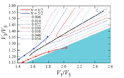
Figure 2: Contour plot of the FQHE gap as a function of $V_{1}/V_{5}$ and $V_{3}/V_{5}$. The black line marks the maximum of the overlap of the ground state wave function and the Pfaffian function. The lines with dots depict the effect of the finite width of a 2D layer. Here the red line corresponds to filling factor $\nu=5/2$, which is the same as $\nu=1/2$ at the $n=1$ Landau level, while the blue line corresponds to $\nu=1/2$ at the $n=0$ Landau level. The dots denote width $w/\ell_{0}=0,1,2,3,4$ (from right to left). The compression region is shaded blue. Reproduced with permission from Storni et al. (2010).

III Monolayer and bilayer graphene in a strong magnetic field

III.1 Graphene monolayer

The graphene is a monolayer of carbon atoms Wallace (1947); Novoselov et al. (2004), which form the 2D honeycomb crystal structure with two sublatices, say A and B [see Fig. 3(a)] Abergel et al. (2010). The corresponding electron band structure has two valleys at two inequivalent points, $K=(2\pi/a)(\frac{1}{3},\frac{1}{\sqrt{3}})$ and $K^{\prime}=(2\pi/a)(\frac{2}{3},0)$, in the reciprocal space [see Fig. 3(b)]. Here $a=0.246$ nm is the lattice constant. The unique property of graphene is that the low-energy dispersion at each valley is determined by the massless Hamiltonian of the Dirac type (Dirac fermions) Castro Neto et al. (2009); Geim and Novoselov (2007); Abergel et al. (2010)

$${\cal H}_{\xi}=\xi v_{\rm F}\left(\begin{array}[]{cc}0&p_{-}\\ p_{+}&0\end{array}\right),$$ (37)

where $\xi$ is the valley index, which is 1 at the $K$ valley and -1 at the $K^{\prime}$ valley, $p_{-}=p_{x}-{\rm i}p_{y}$, $p_{+}=p_{x}+{\rm i}p_{y}$, and $v_{\rm F}\approx 10^{6}$ m/s is the Fermi velocity. The corresponding eigenfunctions of the Hamiltonian (37) have two components due to two sublattices, $A$ and $B$, of the graphene honeycomb lattice. The wave functions are expressed as $(\psi_{A},\psi_{B})^{T}$ for valley $K$ and $(\psi_{B},\psi_{A})^{T}$ for valley $K^{\prime}$, where $\psi_{A}$ and $\psi_{B}$ correspond to sublattices $A$ and $B$, respectively.

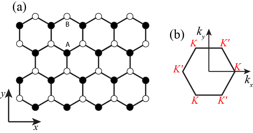
Figure 3: (a) Honeycomb crystal structure of graphene monolayer. Two equivalent sublattices A and B are marked by open and filled dots. (b) The first Brillouin zone of monolayer graphene. Two valley $K$ and $K^{\prime}$ are also shown.

The Landau level of electrons in graphene can be found from Hamiltonian (37) by replacing the electron momentum $\vec{p}$ with the generalized momentum $\vec{\pi}=\vec{p}+e\vec{A}/c$,

$${\cal H}_{\xi}=\xi v_{\rm F}\left(\begin{array}[]{cc}0&\pi_{-}\\ \pi_{+}&0\end{array}\right).$$ (38)

Then the eigenfunctions of the Hamiltonian (38) have the following form

$$\Psi^{K}_{n,m}=\left(\begin{array}[]{c}\psi_{A}\\ \psi_{B}\end{array}\right)=C_{n}\left(\begin{array}[]{c}{\rm sgn}(n){\rm i}^{|n|-1}\phi_{|n|-1,m}\\ {\rm i}^{|n|}\phi_{|n|,m}\end{array}\right),$$ (39)

for the valley $K$ ($\xi=1$) and

$$\Psi^{K^{\prime}}_{n,m}=\left(\begin{array}[]{c}\psi_{B}\\ \psi_{A}\end{array}\right)=C_{n}\left(\begin{array}[]{c}{\rm sgn}(n){\rm i}^{|n|-1}\phi_{|n|-1,m}\\ {\rm i}^{|n|}\phi_{|n|,m}\end{array}\right),$$ (40)

for the valley $K^{\prime}$ ($\xi=-1$). Here $C_{n}=1$ for $n=0$ and $C_{n}=1/\sqrt{2}$ for $n\neq 0$ and

$$\mbox{sgn}(n)=\left\{\begin{array}[]{cc}0&(n=0)\\ 1&(n>0)\\ -1&(n<0).\end{array}\right.,$$ (41)

where the positive and negative values of $n$ correspond to the conduction and valence bands, respectively. The corresponding Landau energy spectrum takes the form McClure (1956); Castro Neto et al. (2009); Goerbig (2011)

$$\varepsilon_{n}=\hbar\omega_{B}\mbox{sgn}(n)\sqrt{|n|},$$ (42)

where $\omega_{B}=\sqrt{2}v_{\rm F}/\ell_{0}$ and $\ell_{0}=\sqrt{\hbar/eB}$ is the magnetic length.

Summarizing, we can say that there are two types of Landau levels in graphene. The first one corresponds to $n=0$. In this case the wave function is

$$\Psi^{K}_{n=0,m}=\left(\begin{array}[]{c}0\\ \phi_{0,m}\end{array}\right).$$ (43)

This wave function consists of only the $\phi_{0,m}$ Landau function of a conventional system. The interacting electron system at $n=0$ graphene Landau level is therefore identical to the interacting electron system in $n=0$ Landau level of the conventional system.

The second class of graphene Landau levels correspond to $n\neq 0$. In this case the wave function is

$$\Psi^{K}_{n,m}=\frac{1}{\sqrt{2}}\left(\begin{array}[]{c}{\rm sgn}(n){\rm i}^{|n|-1}\phi_{|n|-1,m}\\ {\rm i}^{|n|}\phi_{|n|,m}\end{array}\right).$$ (44)

Now, the graphene wave function is the mixture of $n$ and $n-1$ Landau wave functions of a conventional electron system.

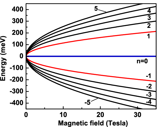
Figure 4: The first few Landau levels of graphene monolyaer as a function of perpendicular magnetic field. The Landau levels are labeled with integer index $n$, where positive and negative $n$ correspond to the conduction and valence bands, respectively. The red and blue lines mark the Landau levels for which the FQHE can be observed.

For Dirac fermions in graphene, the unique feature of the Landau levels (42) is their square-root dependence on both the magnetic field $B$ and the Landau level index $n$. This behavior is different from that in conventional semiconductor 2D systems with the parabolic energy dispersion discussed above, where the Landau levels have linear dependence on both the magnetic field and the Landau level index [see Eq. (7)]. The Landau level of graphene are shown in Fig. 4 as a function of the magnetic field. Here the positive and negative Landau level indices $n$ correspond to the conduction and valence bands, respectively. These unique properties of the Landau levels of Dirac fermions in graphene result in the unconventional Quantum Hall Effect in graphene with quantum Hall plateaus at filling factors $4\left(n+\frac{1}{2}\right)$ Novoselov et al. (2004); Zhang et al. (2005).

III.2 Bilayer graphene

The bilayer graphene consists of two coupled graphene monolayers McCann and Fal’ko (2006); McCann and Koshino (2013), which can be in two possible main stackings: (i) AA stacking and (ii) Bernal (AB) stacking, which are shown schematically in Fig. 5.

For bilayer graphene with AA stacking, there is a interlayer coupling between the Landau levels of two layers with the same Landau level indices. Such coupling changes the energies of the Landau levels of graphene monolayers, but does not affect the wavefunctions of the layers. Therefore, the bilayer graphene Haldane pseudopotentials, which characterize the electron-electron interaction properties, are completely identical to the corresponding pseudoptentials of monolayer graphene.

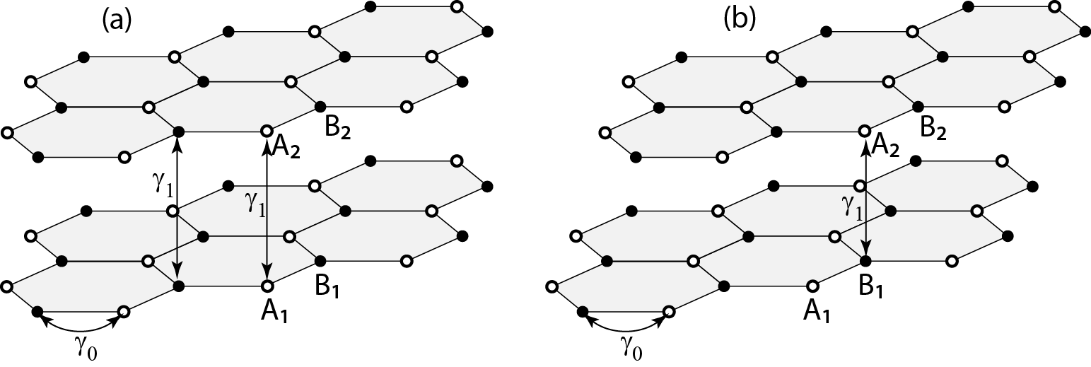
Figure 5: (a) Bilayer graphene with AA stacking. Here the interlayer hopping couples sublattice A (B) in the top layer with sublattice A (B) in the bottom layer. (b) Bilayer graphene with AB staking. For such staking, sublattice A (B) in the top layer is coupled to sublattice B (A) in the bottom layer.

For bilayer graphene with Bernal (AB) stacking, the interlayer coupling strongly modifies the properties of the Landau level in the system. The corresponding Hamiltonian for valley $\xi=\pm 1$ has the form McCann and Fal’ko (2006)

$${\cal H}_{\xi}^{(AB)}=\xi\left(\begin{array}[]{cccc}\frac{U}{2}&v_{\rm F}\pi_{-}&0&0\\ v_{\rm F}\pi_{+}&\frac{U}{2}&\xi\gamma_{1}&0\\ 0&\xi\gamma_{1}&-\frac{U}{2}&v_{\rm F}\pi_{-}\\ 0&0&v_{\rm F}\pi_{+}&-\frac{U}{2}\end{array}\right).$$ (45)

where $U$ is the inter-layer bias voltage and $\gamma_{1}\approx 400$ meV is the interlayer hopping integral. The corresponding wave functions have the structure of $(\psi_{A_{1}},\psi_{B_{1}},\psi_{A_{2}},\psi_{B_{2}})^{T}$, where $A_{1}$, $B_{1}$ correspond to the lower monolayer and $A_{2}$, $B_{2}$ correspond to the upper monolayer. From Hamiltonian (45), the Landau level wave functions are

$$\Psi^{\rm(bi)}_{n,m}=\left(\begin{array}[]{c}\xi C_{1}\phi_{n-1,m}\\ C_{2}\phi_{n,m}\\ C_{3}\phi_{n,m}\\ \xi C_{4}\phi_{n+1,m}\end{array}\right),$$ (46)

where $C_{1}$, $C_{2}$, $C_{3}$, and $C_{4}$ are constants. The wave functions in the bilayer graphene with AB stacking are therefore the mixtures of the conventional Landau wavefunctions with indices $n-1$, $n$, and $n+1$.

In Eq. (46) the Landau index $n$ can take the following values: $n=-1,0,1,\ldots$. Here we assume that if the index of the Landau wave function, $\phi_{n,m}$, is negative then the function is identically zero, which means that $\phi_{-2,m}\equiv 0$ and $\phi_{-1,m}\equiv 0$. Hence, for $n=-1$, the wave function (46) is just $\Psi^{\rm(bi)}_{-1,m}=(0,0,0,\phi_{0,m})$, i.e., the coefficients $C_{1}$, $C_{2}$, $C_{3}$ are zero. Therefore, there is only one energy level corresponding to $n=-1$. For $n=0$, the wave function (46) has zero coefficient $C_{1}$ and, correspondingly, there are only three energy levels.

For $n>0$, there are four eigenvalues of the Hamiltonian (45), corresponding to four Landau levels in a bilayer graphene at a given valley $\xi=\pm 1$. The eigenvalue equation, which determines the Landau levels is written as Pereira et al. (2007)

$$\left[\left(\varepsilon+\xi u\right)^{2}-2n\right]\left[\left(\varepsilon-\xi u\right)^{2}-2(n+1)\right]=\tilde{\gamma}_{1}^{2}\left[\varepsilon^{2}-u^{2}\right],$$ (47)

where $\varepsilon$ is the energy of the Landau level in units of $\epsilon_{B}$, $\epsilon_{B}=\hbar v_{\rm F}/\ell_{0}$, $\tilde{\gamma}_{1}=\gamma_{1}/\epsilon_{B}$, and $u=U/\epsilon_{B}$.

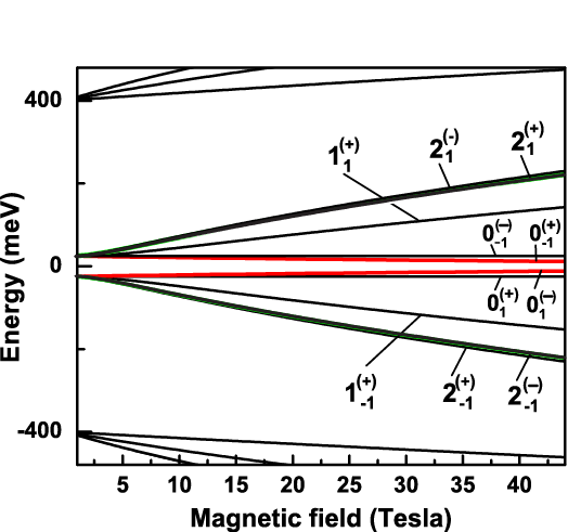
Figure 6: A few lowest Landau levels of bilayer graphene as a function of the magnetic field. The bilayer graphne has the AB staking. The Landau levels of both $K$ and $K^{\prime}$ are shown. The red lines show special Landau levels, at which the $\nu=1/2$ Pfaffian incompressible state can be realized. The bias voltage is 5 meV and interlayer hopping integral is $\gamma_{1}=400$ meV.

The four Landau levels determined by Eq. (47) have two levels with negative energy (valence band) and two levels with positive energy (conduction band). It is then convenient to label these levels as follows: for a given value of $n$ and a given valley $\xi$ we label the levels as $n^{(\xi)}_{i}$, where $i=-2,-1,1,2$ in the ascending order and the negative and positive values of $i$ correspond to the valence and conduction bands, respectively. Although for $n=0$ there are only three Landau levels and for $n=-1$ there is only one Landau level, it is convenient to combine them in a single set of $n=0$ Landau levels and label them as $0^{(\xi)}_{i}$, where $i=-2,-1,1,2$. Also, the Landau levels of different valleys are related as follows $\epsilon(n^{(\xi)}_{i})=-\epsilon(n^{(-\xi)}_{-i})$.

With the known wave functions (46) of the bilayer graphene Landau levels, the form factor in Eq. (8) for Haldane pseudopotentials can be obtained from the following expression

$$F_{n}(q)=|C_{1}|^{2}L_{n-1}(q^{2}/2)+\left(|C_{2}|^{2}+|C_{3}|^{2}\right)L_{n}(q^{2}/2)+|C_{4}|^{2}L_{n+1}(q^{2}/2).$$ (48)

There are two special Landau levels of bilayer graphene with almost zero energy Apalkov and Chakraborty (2011). The first one corresponds to $n=-1$ with the energy of $\varepsilon=-\xi u$ and the corresponding wave function,

$$\Psi^{\rm(bi)}_{0^{(+)}_{1},m}=\Psi^{\rm(bi)}_{0^{(-)}_{-1},m}=\left(\begin{array}[]{c}0\\ 0\\ 0\\ \phi_{0,m}\end{array}\right).$$ (49)

The wave function consists of only the $n=0$ conventional Landau level wave function. Therefore, the FQHE in this bilayer Landau level is exactly the same as the one in the $0$-th conventional Landau level. For example, we can say that there is no FQHE in the half-filled $0^{(+)}_{1}$ Landau level.

In order to find the half-filled level with possible Pfaffian function as the ground state, the most interesting bilayer Landau level is $0^{(+)}_{-1}$ in the $K$ valley and $0^{(-)}_{1}$ in the $K^{\prime}$ valley Apalkov and Chakraborty (2011). For small values of $U$, the energy of this state is almost zero, $\varepsilon\approx 0$. The wave function of $0^{(+)}_{-1}$ Landau level has the form

$$\Psi^{\rm(bi)}_{0_{-1},m}=\frac{1}{\sqrt{\tilde{\gamma}_{1}^{2}+2}}\left(\begin{array}[]{c}0\\ \sqrt{2}\phi_{0,m}\\ 0\\ \tilde{\gamma}_{1}\phi_{1,m}\end{array}\right)=\frac{1}{\sqrt{\gamma_{1}^{2}+2\epsilon_{B}^{2}}}\left(\begin{array}[]{c}0\\ \sqrt{2}\epsilon_{B}\phi_{0,m}\\ 0\\ \gamma_{1}\phi_{1,m}\end{array}\right).$$ (50)

The wave function is the mixture of $\phi_{0,m}$ and $\phi_{1,m}$ states. For a relatively small magnetic field, $\epsilon_{B}\ll\gamma_{1}$, the wave function becomes $(0,0,0,\psi_{1,m})^{T}$, i.e., it is completely identical to the $n=1$ conventional Landau level. In a large magnetic field, $\epsilon_{B}\gg\gamma_{1}$, the $0^{(+)}_{-1}$ Landau wave function becomes $(0,0,\psi_{0,m},0)^{T}$, i.e., it is the same as $n=0$ conventional Landau level. The interesting aspect of this is that, by varying the magnetic field the electron-electron interactions within the $0^{(+)}_{-1}$ Landau level transform from $n=1$ to the conventional $n=0$ case.

IV Pfaffian states in graphene

IV.1 Graphene monolayer

The electron-electron interactions and correspondingly the nature of the ground state within a given Landau level are determined by the Haldane pseudopotentials, which are defined by the corresponding form factor $F(q)$. For graphene monolayer there are two types of Landau levels: (i) the $n=0$ Landau level and (ii) the $n\neq 0$ levels. For the $n=0$ Landau level, the form factor is given by

$$F_{0}(q)=L_{0}(q^{2}/2)=1.$$ (51)

This is exactly the same form factor as the one for the $n=0$ conventional Landau level, for which there is no $\nu=1/2$ FQHE state. We can then conclude that in the $n=0$ graphene Landau level, there is no incompressible $\nu=1/2$-FQHE state with the Pfaffian function as a ground state wave function. At the same time, all other FHQE states, such as $p/q$ with odd $q$, have exactly the same properties, i.e., the same ground state wave functions and the same excitation gaps, as the ones for the $n=0$ conventional Landau level. This suggests that, as long as there is no inter-Landau level mixing, the electron systems in the $n=0$ graphene Landau level are identical to the systems in the $n=0$ conventional Landau level.

On the other hand, for the $n\neq 0$ graphene Landau level, the form factor is

$$F_{n}(q)=\frac{1}{2}\left(L_{n-1}(q^{2}/2)+L_{n}(q^{2}/2)\right).$$ (52)

For example, for $n=1$, $L_{0}(q^{2}/2)=1$ and $L_{0}(q^{2}/2)=1-q^{2}/2$ and the form factor is $F_{n}(q)=1-q^{2}/4$. In this case the form factor is the mixture of the form factors of $n$ and $n-1$ conventional Landau levels. The electron-electron interactions in this case are completely different from those in conventional systems. One of these differences is related to stability, i.e., the magnitude of the excitation gaps of the conventional FQHE with the filling factor $p/q$, where $q$ is odd. This means that, out of all the graphene Landau levels, including the $n=0$ Landau level, the largest FQHE gaps are realized in the $n=1$ Landau level Apalkov and Chakraborty (2006); Chakraborty and Apalkov (2014). This is different from conventional systems, where the conventional FQHE states have the largest gaps for the $n=0$ Landau level.

Our extensive numerical analyses have established that there is no incompressible $\nu=1/2$ state of the Pfaffian type for $n=0$ and $n=1$ graphene Landau levels Apalkov and Chakraborty (2006). Here, the excitation gap is small and the overlap of the ground state wave function with the Pfaffian function is also small. This analysis has been done without considering inter-Landau level mixing. This mixing can alter the properties of the half-filled Landau level, resulting in the formation of an incompressible state. For example, for conventional systems it was shown that the inter-Landau mixing favors the anti-Pfaffian state over other type of ground states of the half-filled $n=1$ Landau level Rezayi (2017). Also, both for conventional and graphene systems, the Landau level mixing crucially modifies for the $1/2$-FQHE state the Haldane pseudoptentials $V_{1}$, $V_{3}$, and $V_{5}$ Peterson and Nayak (2013). The Landau level mixing is also more pronounced at higher Landau levels. It should be noted that, recent experimental results Kim et al. (2019) indeed suggest that the incompressible $\nu=1/2$ state may be realized in monolayer graphene, albeit in higher $n=3$ Landau level. Here, the inter-Landau mixing can be important and it can be the reason for the incompressible $\nu=1/2$ state being present in the higher Landau level in graphene. Further, the even-denominator incompressible states have been observed experimentally in low Landau levels in graphene within some range of the magnetic fields Zibrov et al. (2018), but the origin of those states is yet to be clearly determined and it can perhaps be related to multicomponent fractional quantum Hall states.

IV.2 Bilayer graphene

For the general bilayer Landau level, the form factor is given by the expression (53) below. Due to the bilayer nature of the system, there are extra parameters which can control the form factor and correspondingly the interaction strength. These parameters are the bias voltage and the direction of the magnetic field, i.e., the component of the magnetic field that is parallel to the bilayer. As we have mentioned above, in bilayer graphene there are two ’special’ Landau levels $0_{-1}^{(+)}$ ($K$ valley) and $0_{1}^{(-)}$ ($K^{\prime}$ valley) for which the Pfaffian function can be the ground state of the half-filled Landau level Apalkov and Chakraborty (2011); Chakraborty and Apalkov (2013).

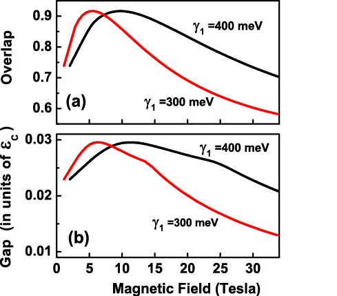
Figure 7: Panel (a): Overlap of the ground state wave function of $\nu=1/2$ state with the Pfaffian state as a function of the magnetic field. Panel (b): the collective excitation gap of the $\nu=1/2$ state as a function of the magnetic field. The data are shown for the Landau level $0_{-1}^{(+)}$ of the bilayer graphene and for two values of the interlayer hopping integral, $\gamma_{1}$. Reproduced with permission from Apalkov and Chakraborty (2011).

Extensive studies of the finite-size system of bilayer graphene have been performed by us in the spherical geometry Haldane (1983); Haldane and Rezayi (1985); Fano et al. (1986). Those studies have revealed that for all bilayer Landau levels, except the ones $0_{-1}^{(+)}$ and $0_{1}^{(-)}$, the overlap of the $\nu=\frac{1}{2}$ ground state with the Pfaffian state is relatively small (less than $0.5$). Therefore, for those Landau levels, the $\nu=\frac{1}{2}$ system is gapless and compressible. A different situation occurs for the Landau levels $0_{-1}^{(+)}$ and $0_{1}^{(-)}$. These levels belong to the $K$ and $K^{\prime}$ valleys, respectively, and have exactly the same interaction properties. Hence, it is enough to consider only one of these levels, e.g., $0_{-1}^{(+)}$, as for the other Landau level, $0_{1}^{(-)}$, the results are exactly the same.

For the $0_{-1}^{(+)}$ Landau level the form factor is

$$F_{0_{-1}}(q)=\left[\frac{\gamma_{1}^{2}}{\gamma_{1}^{2}+2\epsilon_{B}^{2}}\right]L_{1}(q^{2}/2)+\left[\frac{2\epsilon_{B}^{2}}{\gamma_{1}^{2}+2\epsilon_{B}^{2}}\right]L_{0}(q^{2}/2).$$ (53)

The strength of magnetic field is determined by the parameter $\epsilon_{B}$. With increasing magnetic field, i.e., with increasing $\epsilon_{B}$, the form factor of the $0_{-1}^{(+)}$ level goes through the following main regions: (i) for small $B$, $\epsilon_{B}\ll\gamma_{1}$, the form factor is $L_{1}(q^{2}/2)$ and identical to the one of the $n=1$ conventional Landau level; (ii) at $\epsilon_{B}=\gamma_{1}/\sqrt{2}$, the form factor is $\frac{1}{2}[L_{0}(q^{2}/2)+L_{1}(q^{2}/2)]$ and is the same as the one of the $n=1$ Landau level of monolayer graphene; (iii) at $\epsilon_{B}\gg\gamma_{1}$, the form factor is $L_{0}(q^{2}/2)$ and is the same as the one of the $n=0$ conventional Landau level.

Since the $\nu=1/2$ incompressible state is realized only in the $n=1$ conventional Landau level, then for bilayer graphene, the $\nu=1/2$ Pfaffian state should be observed only for relatively small values of the magnetic field. At the same time, it so happens that as a function of the magnetic field, the characteristics of the $\nu=1/2$ system is not monotonic. In Fig. 7 (a) the overlap of the $\nu=1/2$ wave function with the Pfaffian function is shown as a function of the magnetic field. The calculations were done in a spherical geometry for $N_{e}=14$ electron system. The overlap has a maximum at a finite magnetic field. The position of the maximum depends on the interlayer hopping integral, $\gamma$. For example, for $\gamma=400$ meV, the maximum overlap occurs for $\approx 10$ T. The profile of the overlap is also correlated with the gap of the collective excitation of the system [see Fig. 7( b)]. The energy gap also has a maximum at a finite magnetic field. Since in a small magnetic field, $B\rightarrow 0$, the $0_{-1}^{(+)}$ bilayer Landau system is equivalent to $n=1$ conventional Landau systems, we are allowed to conclude that the stability of the Pfaffian $\nu=\frac{1}{2}$ state in bilayer graphene can be increased compared to that of the conventional systems.

The position of the maximum in Fig. 7 can be analyzed further by looking at some dimensionless quantities. For instance, in dimensionless units the maximum is achieved at $\gamma_{1}/\epsilon_{B}\approx 4.9$. This means that, in terms of the magnetic field, the position of the maximum of the overlap is approximately proportional to $\gamma_{1}$, which is also seen in Fig. 7.

Using the phase diagram shown in Fig. 2, which characterizes the stability of the $\nu=1/2$ state described by the Pfaffian function, we can illustrate how the interaction parameters in the $0_{-1}^{(+)}$ Landau level change with the magnetic field [see Fig. 8]. For a small magnetic field, the ground state of the system is well described by the Pfaffian function, while the overlap and the corresponding excitation gap reach their maximum at intermediate values of the magnetic field and finally, for a large magnetic field, $>100$ T, the electron system becomes compressible.

Another parameter that can be used to control the stability of the Pfaffian ground state, is the magnetic field that is parallel to the 2D layer Chakraborty and Apalkov (2013). The reason why the parallel magnetic field changes the wave functions and the interaction potential is due to the bilayer nature of the system. In this case the system has extra dynamics in the $z$ direction, which is described in the model as an inter-layer hopping. The parallel component of the magnetic field can be introduced into the Hamiltonian of bilayer graphene through a Peierls substitution as an extra position-dependent phase factor in the inter-layer hopping integral. The details of that study can be found elsewhere Chakraborty and Apalkov (2013).

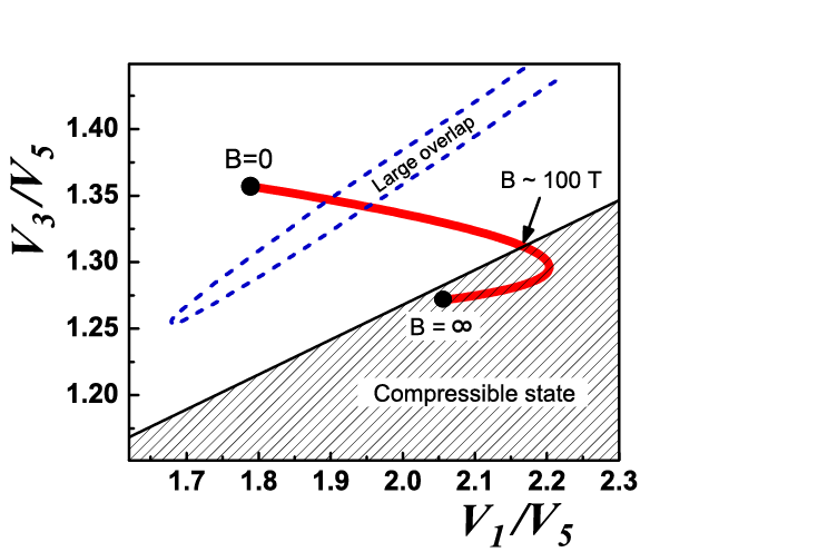
Figure 8: Trajectory of the inter-electron interaction with varying magnetic field. The trajectory is shown by a solid red line in the plane $(V_{1}/V_{5})-(V_{3}/V_{5})$ for the Landau level $0_{-1}^{(+)}$ of the bilayer graphene. The initial point of the trajectory (at $B=0$) corresponds to the conventional system at $n=1$ Landau level, while the final point (at $B=\infty$) corresponds to the conventional system at the $n=0$ LL. The hatched region illustrates the compressible $\nu=1/2$ state, while the blank region corresponds to the incompressible $\nu=1/2$ state following the Ref. Storni et al. (2010) and Fig. 2. The crossing of the boundary between the compressible and incompressible states occurs at $B\sim 100$ Tesla for the interlayer hopping integral $\gamma_{1}=400$ meV. The blue dashed line shows the region of large overlap of the ground state wave function with the Pfaffian function. Reproduced with permission from Apalkov and Chakraborty (2011).

The effect of the parallel component of the magnetic field is illustrated in Fig. 9, where the parameters $V_{1}/V_{5}$ and $V_{3}/V_{5}$ are shown as a function of the perpendicular component of the magnetic field and for different values of its parallel component. The most stable Pfaffian state is illustrated by the dashed lines. The results demonstrate that with increasing parallel component of the magnetic field the values of pseudopotentials, which correspond to the most stable Pfaffian state, are realized for smaller values of the perpendicular component of the magnetic field. Therefore, the parallel component of the magnetic field can be used to tune the stability of the Pfaffian state and the magnetic field where it can be realized.

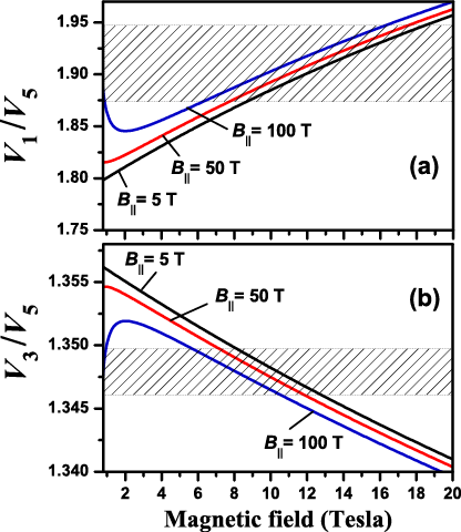
Figure 9: Ratios of pseudopotentials at two values of angular momentum $V_{1}/V_{5}$ [panel (a)] and $V_{3}/V_{5}$ [panel (b)] are shown as the function of perpendicular component of magnetic field and for different parallel components of magnetic field, $B_{\parallel}=5$ T, 50 T, and 100 T. The data are shown for Landau level $0_{-1}^{(+)}$ of bilayer graphene. The hatched regions correspond to the values of pseudopotentials for which the large overlap of the ground state wave function with the Pfaffian function and large excitation gap of incompressible ground state are achieved. Reproduced with permission from Chakraborty and Apalkov (2013).

IV.3 Finding the Pfaffians

Even-denominator fractional quantum Hall effect has been observed experimentally in bilayer graphene Zibrov et al. (2017); Li et al. (2017). It was found that the corresponding states were spin-polarized and it was suggested that they are Pfaffian or anti-Pfaffian states corresponding to the half-filled Landau level. Such states were observed at high energy bilayer Landau levels that are a mixture of the $n=1$ and $n=0$ conventional Landau levels. It was noted that the FQHE was observed only at the filling factor $\nu=3/2$, but not at $\nu=1/2$ and $5/2$ Li et al. (2017). This observation illustrates the high sensitivity of the half-filled incompressible states to the structure of the electron wave functions which determine the electron-electron interaction potentials. Also the measured activation gap of the half-filled incompressible state was several times larger than the largest gaps measured in the GaAs systems Zibrov et al. (2017), which also illustrates that the half-filled FHQE state is much more stable in bilayer graphene then in conventional electron systems. It was observed that the stability of the experimentally found $1/2$-FQHE states is sensitive to both the magnitude of the magnetic field and the perpendicular component of the electric field. With variation of these parameters, transitions from the compressible to the incompressible states have been observed Li et al. (2017). Such a behavior is in complete accord with our theoretical predictions elaborated in the previous section.

V Conclusion

Two-dimensional electron systems placed in a strong magnetic field can support charged excitations with fractional charge and non-Abelian statistics. These excitations are possible only due to the nature of electron-electron interactions of a special type. The example of such a system is an electron gas in a given Landau level that is only half filled. Under a special profile of the interaction potential, the ground state of the $\nu=1/2$-Landau level is described by the Pfaffian function. Here the profile of interaction potential is determined by the form factor of the corresponding Landau level. As a result, for the conventional electron systems, the incompressible $\nu=1/2$-FQHE state is realized only in the $n=1$ Landau level, but for the graphene monolayer which has the relativistic-like low-energy dispersion (that of the Dirac fermions), there is no incompressible $\nu=1/2$ Pfaffian state in any Landau level. This theoretical conclusion is based on the properties of electrons within a given Landau level, without considering the admixture of other Landau levels. The Landau level mixing, which is especially relevant for higher Landau levels, can modify the properties of the half-filled Landau states [see Rezayi (2017); Rezayi and Simon (2011); Simon and Rezayi (2013); Pakrouski et al. (2015); Peterson and Nayak (2013); Luo and Chakraborty (2017). It can also open up the possibility to observe the $\nu=1/2$-FQHE in higher Landau levels in graphene Kim et al. (2019).

In this context, bilayer graphene is truly unique because for bilayer graphene with AB staking, there are two special Landau levels: one in the $K$ valley and another one in the $K^{\prime}$ valley, for which, there is a range of magnetic fields where the $\nu=1/2$ ground state is determined by the Pfaffian function. Stability of such a ground state, i.e., its collective excitation gap, depends on the magnetic field and for a finite magnetic field, the $\nu=1/2$-FQHE state becomes even more stable than the corresponding state in a conventional electron system. Another important property of bilayer graphene is that there are external parameters, such as the bias voltage and the in-plane magnetic field, that can change the inter-electron interaction strength within a given Landau level and correspondingly change the properties of the $\nu=1/2$ Pfaffian state.

In addition to the unique properties of the $\nu=1/2$ Pfaffian state, the system with half filling of a given Landau level has another interesting feature. In particular, when the projection on a given Landau level is considered, i.e., only the states within this Landau level are taken into account with inter-landau level mixing, then the system itself has a particle-hole symmetry. It means that it can be described either as the $\nu=1/2$ particle (electron) system or the $\nu=1/2$ hole system. The Pfaffian function, which describes the $\nu=1/2$ particle system, is not invariant under the exchange of particles and holes. When the particle-hole symmetry operation is applied to the Pfaffian function it generates the Pfaffian conjugated function, which is known as the anti-Pfaffian Levin et al. (2007); Lee et al. (2007). The anti-Pfaffian function is given by

$$\Psi_{\mbox{aPf}}=\mbox{Pf}\left[\frac{z_{i}-z_{j}}{(z_{i}^{*}-z_{j}^{*})^{2}}\right]\prod_{i<j}(z_{i}-z_{j})^{2}\exp\left(-\sum_{i}\frac{z_{i}^{2}}{4\ell_{0}^{2}}\right).$$ (54)

In addition to the Pfaffian and anti-Pfaffian functions, another type of function have been proposed in the literature. It is called the PH-Pfaffian and is symmetric with respect to the particle-hole symmetry operator Son (2015). The PH-Pfaffian is given by the following expression

$$\Psi_{\mbox{PH-Pf}}=\mbox{Pf}\left[\frac{1}{z_{i}^{*}-z_{j}^{*}}\right]\prod_{i<j}(z_{i}-z_{j})^{2}\exp\left(-\sum_{i}\frac{z_{i}^{2}}{4\ell_{0}^{2}}\right).$$ (55)

All these functions, Pfaffian, anti-Pfaffian, and PH-Pfaffian, are of the superconductor-type with Cooper pairing but having different pairing symmetries. The corresponding charged excitations are non-Abelian anyons. Discussion of the conditions under which different Pfaffian-type functions are to be realized and their properties can be found in the literature Simon and Rezayi (2013); Rezayi and Simon (2011); Zaletel et al. (2015); Rezayi (2017); Sodemann and MacDonald (2013); Pakrouski et al. (2015); Peterson and Nayak (2013); Wójs et al. (2010); Bonderson et al. (2011); Antonić et al. (2018); Hsin et al. (2020); Rezayi et al. (2021). Confirmation of the presence of Pfaffian functions in half-filled FQHE will provide another open door to our understanding of this distinctive many-body phenomena that have enthralled us for more than four decades. Additionally, it would be equally exciting to watch that the work of Cayley and Pfaff finally see the light of day through bilayer graphene.

References

- Abergel et al. (2010) Abergel, D.S.L., Apalkov, V., Berashevich, J., Ziegler, K., Chakraborty, T., 2010. Properties of graphene: A theoretical perspective. Adv. Phys. 59, 261–482.
- Antonić et al. (2018) Antonić, L., Vučičević, J., Milovanović, M.V., 2018. Paired states at 5/2: Particle-hole pfaffian and particle-hole symmetry breaking. Physical Review B 98, 115107. URL: https://link.aps.org/doi/10.1103/PhysRevB.98.115107, doi:10.1103/PhysRevB.98.115107.
- Apalkov and Chakraborty (2006) Apalkov, V.M., Chakraborty, T., 2006. Fractional quantum hall states of dirac electrons in graphene. Physical Review Letters 97, 126801. URL: https://link.aps.org/doi/10.1103/PhysRevLett.97.126801, doi:10.1103/PhysRevLett.97.126801.
- Apalkov and Chakraborty (2011) Apalkov, V.M., Chakraborty, T., 2011. Stable pfaffian state in bilayer graphene. Physical Review Letters 107, 186803. URL: https://link.aps.org/doi/10.1103/PhysRevLett.107.186803, doi:10.1103/PhysRevLett.107.186803.
- Apalkov et al. (2001) Apalkov, V.M., Chakraborty, T., Pietiläinen, P., Niemelä, K., 2001. Half-polarized quantum hall states. Physical Review Letters 86, 1311–1314. URL: https://link.aps.org/doi/10.1103/PhysRevLett.86.1311, doi:10.1103/PhysRevLett.86.1311.
- Ashcroft and Mermin (1976) Ashcroft, W., Mermin, D., 1976. Solid State Physics. Cengage, Boston, MA.
- Ayukaryana et al. (2021) Ayukaryana, N.R., Fauzi, M.H., Hasdeo, E.H., 2021. The quest and hope of majorana zero modes in topological superconductor for fault-tolerant quantum computing: An introductory overview. AIP Conference Proceedings 2382, 020007. URL: https://aip.scitation.org/doi/abs/10.1063/5.0059974, doi:10.1063/5.0059974.
- Bajdich et al. (2008) Bajdich, M., Mitas, L., Wagner, L.K., Schmidt, K.E., 2008. Pfaffian pairing and backflow wavefunctions for electronic structure quantum monte carlo methods. Physical Review B 77, 115112. URL: https://link.aps.org/doi/10.1103/PhysRevB.77.115112, doi:10.1103/PhysRevB.77.115112.
- Bonderson et al. (2011) Bonderson, P., Gurarie, V., Nayak, C., 2011. Plasma analogy and non-abelian statistics for ising-type quantum hall states. Physical Review B 83, 075303. URL: https://link.aps.org/doi/10.1103/PhysRevB.83.075303, doi:10.1103/PhysRevB.83.075303.
- Bouchaud et al. (1988) Bouchaud, J., Georges, A., Lhuillier, C., 1988. Pair wave functions for strongly correlated fermions and their determinantal representation. J. Phys. France 49, 553–559. URL: https://doi.org/10.1051/jphys:01988004904055300.
- Castro Neto et al. (2009) Castro Neto, A.H., Guinea, F., Peres, N.M.R., Novoselov, K.S., Geim, A.K., 2009. The electronic properties of graphene. Reviews of Modern Physics 81, 109–162. URL: https://link.aps.org/doi/10.1103/RevModPhys.81.109, doi:10.1103/RevModPhys.81.109.
- Cayley (1847) Cayley, A., 1847. Sur les de’terminants gauches. Crelle’s J. 38, 93.
- Chakraborty and Apalkov (2014) Chakraborty, T., Apalkov, V., 2014. Aspects of the Fractional Quantum Hall Effect in Graphene. Springer International Publishing, Cham. pp. 251–300. URL: https://doi.org/10.1007/978-3-319-02633-6_8, doi:10.1007/978-3-319-02633-6_8.
- Chakraborty and Apalkov (2013) Chakraborty, T., Apalkov, V.M., 2013. Traits and characteristics of interacting dirac fermions in monolayer and bilayer graphene. Solid State Communications 175-176, 123–131. URL: https://www.sciencedirect.com/science/article/pii/S0038109813001579, doi:https://doi.org/10.1016/j.ssc.2013.04.002.
- Chakraborty and Pietiläinen (1995) Chakraborty, T., Pietiläinen, P., 1995. The Quantum Hall Effect. Springer, New York.
- Chakraborty et al. (1986) Chakraborty, T., Pietiläinen, P., Zhang, F.C., 1986. Elementary excitations in the fractional quantum hall effect and the spin-reversed quasiparticles. Physical Review Letters 57, 130–133. URL: https://link.aps.org/doi/10.1103/PhysRevLett.57.130, doi:10.1103/PhysRevLett.57.130.
- Chakraborty and Zhang (1984) Chakraborty, T., Zhang, F.C., 1984. Role of reversed spins in the correlated ground state for the fractional quantum hall effect. Physical Review B 29, 7032–7033. URL: https://link.aps.org/doi/10.1103/PhysRevB.29.7032, doi:10.1103/PhysRevB.29.7032.
- Crilly (2016) Crilly, T., 2016. Half-determinants: an historical note. The Mathematical Gazette 66, 316–316. URL: https://www.cambridge.org/core/article/halfdeterminants-an-historical-note/FC1A9BB82E0DA1C074C181826E3E28F4, doi:10.2307/3615529.
- Das Sarma et al. (2005) Das Sarma, S., Freedman, M., Nayak, C., 2005. Topologically protected qubits from a possible non-abelian fractional quantum hall state. Physical Review Letters 94, 166802. URL: https://link.aps.org/doi/10.1103/PhysRevLett.94.166802, doi:10.1103/PhysRevLett.94.166802.
- Fano et al. (1986) Fano, G., Ortolani, F., Colombo, E., 1986. Configuration-interaction calculations on the fractional quantum hall effect. Physical Review B 34, 2670–2680. URL: https://link.aps.org/doi/10.1103/PhysRevB.34.2670, doi:10.1103/PhysRevB.34.2670.
- Geim and Novoselov (2007) Geim, A.K., Novoselov, K.S., 2007. The rise of graphene. Nature Materials 6, 183–191. URL: https://doi.org/10.1038/nmat1849, doi:10.1038/nmat1849.
- Goerbig (2011) Goerbig, M.O., 2011. Electronic properties of graphene in a strong magnetic field. Reviews of Modern Physics 83, 1193–1243. URL: https://link.aps.org/doi/10.1103/RevModPhys.83.1193, doi:10.1103/RevModPhys.83.1193.
- Greiter (2011) Greiter, M., 2011. Landau level quantization on the sphere. Physical Review B 83, 115129. URL: https://link.aps.org/doi/10.1103/PhysRevB.83.115129, doi:10.1103/PhysRevB.83.115129.
- Greiter et al. (1991) Greiter, M., Wen, X.G., Wilczek, F., 1991. Paired hall state at half filling. Physical Review Letters 66, 3205–3208. URL: https://link.aps.org/doi/10.1103/PhysRevLett.66.3205, doi:10.1103/PhysRevLett.66.3205.
- Greiter et al. (1992) Greiter, M., Wen, X.G., Wilczek, F., 1992. Paired hall states. Nuclear Physics B 374, 567–614. URL: https://www.sciencedirect.com/science/article/pii/055032139290401V, doi:https://doi.org/10.1016/0550-3213(92)90401-V.
- Haldane (1983) Haldane, F.D.M., 1983. Fractional quantization of the hall effect: A hierarchy of incompressible quantum fluid states. Physical Review Letters 51, 605–608. URL: https://link.aps.org/doi/10.1103/PhysRevLett.51.605, doi:10.1103/PhysRevLett.51.605.
- Haldane (1987) Haldane, F.D.M., 1987. The Quantum Hall Effect. Springer, New York.
- Haldane (2011) Haldane, F.D.M., 2011. Geometrical description of the fractional quantum hall effect. Physical Review Letters 107, 116801. URL: https://link.aps.org/doi/10.1103/PhysRevLett.107.116801, doi:10.1103/PhysRevLett.107.116801.
- Haldane and Rezayi (1985) Haldane, F.D.M., Rezayi, E.H., 1985. Finite-size studies of the incompressible state of the fractionally quantized hall effect and its excitations. Physical Review Letters 54, 237–240. URL: https://link.aps.org/doi/10.1103/PhysRevLett.54.237, doi:10.1103/PhysRevLett.54.237.
- Hall (1879) Hall, E.H., 1879. On a new action of the magnet on electric currents. American Journal of Mathematics 2, 287–292. URL: http://www.jstor.org/stable/2369245, doi:10.2307/2369245.
- Halperin and Jain (2020) Halperin, B., Jain, J. (Eds.), 2020. Fractional Quantum Hall Effects: New Developments. World Scientific.
- Halperin et al. (1993) Halperin, B.I., Lee, P.A., Read, N., 1993. Theory of the half-filled landau level. Physical Review B 47, 7312–7343. URL: https://link.aps.org/doi/10.1103/PhysRevB.47.7312, doi:10.1103/PhysRevB.47.7312.
- Halton (1966) Halton, J.H., 1966. A combinatorial proof of cayley’s theorem on pfaffians. Journal of Combinatorial Theory 1, 224.
- Hsin et al. (2020) Hsin, P.S., Lin, Y.H., Paquette, N.M., Wang, J., 2020. Effective field theory for fractional quantum hall systems near . Physical Review Research 2, 043242. URL: https://link.aps.org/doi/10.1103/PhysRevResearch.2.043242, doi:10.1103/PhysRevResearch.2.043242.
- Hurd (1972) Hurd, C.M., 1972. The Hall Effect in Metals and Alloys. Plenum.
- Ivanov (2001) Ivanov, D.A., 2001. Non-abelian statistics of half-quantum vortices in -wave superconductors. Physical Review Letters 86, 268–271. URL: https://link.aps.org/doi/10.1103/PhysRevLett.86.268, doi:10.1103/PhysRevLett.86.268.
- Kim et al. (2019) Kim, Y., Balram, A.C., Taniguchi, T., Watanabe, K., Jain, J.K., Smet, J.H., 2019. Even denominator fractional quantum hall states in higher landau levels of graphene. Nature Physics 15, 154–158. URL: https://doi.org/10.1038/s41567-018-0355-x, doi:10.1038/s41567-018-0355-x.
- Kitaev (2003) Kitaev, A.Y., 2003. Fault-tolerant quantum computation by anyons. Annals of Physics 303, 2–30. URL: https://www.sciencedirect.com/science/article/pii/S0003491602000180, doi:https://doi.org/10.1016/S0003-4916(02)00018-0.
- Kittel (2005) Kittel, C., 2005. Introduction to Solid State Physics. Wiley, Hoboken, NJ.
- von Klitzing et al. (2020) von Klitzing, K., Chakraborty, T., Kim, P., Madhavan, V., Dai, X., McIver, J., Tokura, Y., Savary, L., Smirnova, D., Rey, A.M., Felser, C., Gooth, J., Qi, X., 2020. 40 years of the quantum hall effect. Nature Reviews Physics 2, 397–401. URL: https://doi.org/10.1038/s42254-020-0209-1, doi:10.1038/s42254-020-0209-1.
- Klitzing (2017) Klitzing, K.v., 2017. Quantum hall effect: Discovery and application. Annual Review of Condensed Matter Physics 8, 13–30. URL: https://www.annualreviews.org/doi/abs/10.1146/annurev-conmatphys-031016-025148, doi:10.1146/annurev-conmatphys-031016-025148.
- Klitzing et al. (1980) Klitzing, K.v., Dorda, G., Pepper, M., 1980. New method for high-accuracy determination of the fine-structure constant based on quantized hall resistance. Physical Review Letters 45, 494–497. URL: https://link.aps.org/doi/10.1103/PhysRevLett.45.494, doi:10.1103/PhysRevLett.45.494.
- Landau and Lifshitz (1965) Landau, L.D., Lifshitz, E.M., 1965. Quantum Mechanics: Non-Relativistic Theory. Pergamon Press, Oxford and New York.
- Laughlin (1983) Laughlin, R.B., 1983. Anomalous quantum hall effect: An incompressible quantum fluid with fractionally charged excitations. Physical Review Letters 50, 1395–1398. URL: https://link.aps.org/doi/10.1103/PhysRevLett.50.1395, doi:10.1103/PhysRevLett.50.1395.
- Lee et al. (2007) Lee, S.S., Ryu, S., Nayak, C., Fisher, M.P.A., 2007. Particle-hole symmetry and the quantum hall state. Physical Review Letters 99, 236807. URL: https://link.aps.org/doi/10.1103/PhysRevLett.99.236807, doi:10.1103/PhysRevLett.99.236807.
- Levin et al. (2007) Levin, M., Halperin, B.I., Rosenow, B., 2007. Particle-hole symmetry and the pfaffian state. Physical Review Letters 99, 236806. URL: https://link.aps.org/doi/10.1103/PhysRevLett.99.236806, doi:10.1103/PhysRevLett.99.236806.
- Li et al. (2017) Li, J.I.A., Tan, C., Chen, S., Zeng, Y., Taniguchi, T., Watanabe, K., Hone, J., Dean, C.R., 2017. Even-denominator fractional quantum hall states in bilayer graphene. Science 358, 648–652. URL: https://www.science.org/doi/abs/10.1126/science.aao2521, doi:doi:10.1126/science.aao2521.
- Luo and Chakraborty (2017) Luo, W., Chakraborty, T., 2017. Pfaffian state in an electron gas with small landau level gaps. Physical Review B 96, 081108. URL: https://link.aps.org/doi/10.1103/PhysRevB.96.081108, doi:10.1103/PhysRevB.96.081108.
- McCann and Fal’ko (2006) McCann, E., Fal’ko, V.I., 2006. Landau-level degeneracy and quantum hall effect in a graphite bilayer. Physical Review Letters 96, 086805. URL: https://link.aps.org/doi/10.1103/PhysRevLett.96.086805, doi:10.1103/PhysRevLett.96.086805.
- McCann and Koshino (2013) McCann, E., Koshino, M., 2013. The electronic properties of bilayer graphene. Reports on Progress in Physics 76, 056503. URL: http://dx.doi.org/10.1088/0034-4885/76/5/056503, doi:10.1088/0034-4885/76/5/056503.
- McClure (1956) McClure, J.W., 1956. Diamagnetism of graphite. Physical Review 104, 666–671. URL: https://link.aps.org/doi/10.1103/PhysRev.104.666, doi:10.1103/PhysRev.104.666.
- Moore and Read (1991) Moore, G., Read, N., 1991. Nonabelions in the fractional quantum hall effect. Nuclear Physics B 360, 362–396. URL: https://www.sciencedirect.com/science/article/pii/055032139190407O, doi:https://doi.org/10.1016/0550-3213(91)90407-O.
- Nayak et al. (2008) Nayak, C., Simon, S.H., Stern, A., Freedman, M., Das Sarma, S., 2008. Non-abelian anyons and topological quantum computation. Reviews of Modern Physics 80, 1083–1159. URL: https://link.aps.org/doi/10.1103/RevModPhys.80.1083, doi:10.1103/RevModPhys.80.1083.
- Novoselov et al. (2004) Novoselov, K.S., Geim, A.K., Morozov, S.V., Jiang, D., Zhang, Y., Dubonos, S.V., Grigorieva, I.V., Firsov, A.A., 2004. Electric field effect in atomically thin carbon films. Science 306, 666–669. URL: https://science.sciencemag.org/content/sci/306/5696/666.full.pdf, doi:10.1126/science.1102896.
- Pakrouski et al. (2015) Pakrouski, K., Peterson, M.R., Jolicoeur, T., Scarola, V.W., Nayak, C., Troyer, M., 2015. Phase diagram of the fractional quantum hall effect: Effects of landau-level mixing and nonzero width. Physical Review X 5, 021004. URL: https://link.aps.org/doi/10.1103/PhysRevX.5.021004, doi:10.1103/PhysRevX.5.021004.
- Pereira et al. (2007) Pereira, J.M., Peeters, F.M., Vasilopoulos, P., 2007. Landau levels and oscillator strength in a biased bilayer of graphene. Physical Review B 76, 115419. URL: https://link.aps.org/doi/10.1103/PhysRevB.76.115419, doi:10.1103/PhysRevB.76.115419.
- Peterson and Nayak (2013) Peterson, M.R., Nayak, C., 2013. More realistic hamiltonians for the fractional quantum hall regime in gaas and graphene. Physical Review B 87, 245129. URL: https://link.aps.org/doi/10.1103/PhysRevB.87.245129, doi:10.1103/PhysRevB.87.245129.
- Prange and Girvin (1987) Prange, R., Girvin, S. (Eds.), 1987. The Quantum Hall Effect. Springer, New York.
- Read and Green (2000) Read, N., Green, D., 2000. Paired states of fermions in two dimensions with breaking of parity and time-reversal symmetries and the fractional quantum hall effect. Physical Review B 61, 10267–10297. URL: https://link.aps.org/doi/10.1103/PhysRevB.61.10267, doi:10.1103/PhysRevB.61.10267.
- Rezayi (2017) Rezayi, E.H., 2017. Landau level mixing and the ground state of the quantum hall effect. Physical Review Letters 119, 026801. URL: https://link.aps.org/doi/10.1103/PhysRevLett.119.026801, doi:10.1103/PhysRevLett.119.026801.
- Rezayi et al. (2021) Rezayi, E.H., Pakrouski, K., Haldane, F.D.M., 2021. Stability of the particle-hole pfaffian state and the -fractional quantum hall effect. Physical Review B 104, L081407. URL: https://link.aps.org/doi/10.1103/PhysRevB.104.L081407, doi:10.1103/PhysRevB.104.L081407.
- Rezayi and Simon (2011) Rezayi, E.H., Simon, S.H., 2011. Breaking of particle-hole symmetry by landau level mixing in the quantized hall state. Physical Review Letters 106, 116801. URL: https://link.aps.org/doi/10.1103/PhysRevLett.106.116801, doi:10.1103/PhysRevLett.106.116801.
- Seiler and Stephens (1991) Seiler, D.G., Stephens, A.E., 1991. CHAPTER 18 - The Shubnikov–de Haas Effect in Semiconductors: A Comprehensive Review of Experimental Aspects. Elsevier. volume 27. pp. 1031–1133. URL: https://www.sciencedirect.com/science/article/pii/B9780444888730500145, doi:https://doi.org/10.1016/B978-0-444-88873-0.50014-5.
- Simon and Rezayi (2013) Simon, S.H., Rezayi, E.H., 2013. Landau level mixing in the perturbative limit. Physical Review B 87, 155426. URL: https://link.aps.org/doi/10.1103/PhysRevB.87.155426, doi:10.1103/PhysRevB.87.155426.
- Sodemann and MacDonald (2013) Sodemann, I., MacDonald, A.H., 2013. Landau level mixing and the fractional quantum hall effect. Physical Review B 87, 245425. URL: https://link.aps.org/doi/10.1103/PhysRevB.87.245425, doi:10.1103/PhysRevB.87.245425.
- Son (2015) Son, D.T., 2015. Is the composite fermion a dirac particle? Physical Review X 5, 031027. URL: https://link.aps.org/doi/10.1103/PhysRevX.5.031027, doi:10.1103/PhysRevX.5.031027.
- Stern (2008) Stern, A., 2008. Anyons and the quantum hall effect—a pedagogical review. Annals of Physics 323, 204–249. URL: https://www.sciencedirect.com/science/article/pii/S0003491607001674, doi:https://doi.org/10.1016/j.aop.2007.10.008.
- Stern and Halperin (2006) Stern, A., Halperin, B.I., 2006. Proposed experiments to probe the non-abelian quantum hall state. Physical Review Letters 96, 016802. URL: https://link.aps.org/doi/10.1103/PhysRevLett.96.016802, doi:10.1103/PhysRevLett.96.016802.
- Stone (1992) Stone, M., 1992. Quantum Hall Effect. World Scientific.
- Storni et al. (2010) Storni, M., Morf, R.H., Das Sarma, S., 2010. Fractional quantum hall state at and the moore-read pfaffian. Physical Review Letters 104, 076803. URL: https://link.aps.org/doi/10.1103/PhysRevLett.104.076803, doi:10.1103/PhysRevLett.104.076803.
- Tsui et al. (1982) Tsui, D.C., Stormer, H.L., Gossard, A.C., 1982. Two-dimensional magnetotransport in the extreme quantum limit. Physical Review Letters 48, 1559–1562. URL: https://link.aps.org/doi/10.1103/PhysRevLett.48.1559, doi:10.1103/PhysRevLett.48.1559.
- Wallace (1947) Wallace, P.R., 1947. The band theory of graphite. Phys. Rev. 71, 622–634.
- Wen (1991) Wen, X.G., 1991. Non-abelian statistics in the fractional quantum hall states. Physical Review Letters 66, 802–805. URL: https://link.aps.org/doi/10.1103/PhysRevLett.66.802, doi:10.1103/PhysRevLett.66.802.
- Willett et al. (1987) Willett, R., Eisenstein, J.P., Störmer, H.L., Tsui, D.C., Gossard, A.C., English, J.H., 1987. Observation of an even-denominator quantum number in the fractional quantum hall effect. Physical Review Letters 59, 1776–1779. URL: https://link.aps.org/doi/10.1103/PhysRevLett.59.1776, doi:10.1103/PhysRevLett.59.1776.
- Willett (2013) Willett, R.L., 2013. The quantum hall effect at 5/2 filling factor. Reports on Progress in Physics 76, 076501. URL: http://dx.doi.org/10.1088/0034-4885/76/7/076501, doi:10.1088/0034-4885/76/7/076501.
- Wójs et al. (2010) Wójs, A., Tőke, C., Jain, J.K., 2010. Landau-level mixing and the emergence of pfaffian excitations for the fractional quantum hall effect. Physical Review Letters 105, 096802. URL: https://link.aps.org/doi/10.1103/PhysRevLett.105.096802, doi:10.1103/PhysRevLett.105.096802.
- Yoshioka (2002) Yoshioka, D., 2002. The Quantum Hall Effect. Springer, New York.
- Zaletel et al. (2015) Zaletel, M.P., Mong, R.S.K., Pollmann, F., Rezayi, E.H., 2015. Infinite density matrix renormalization group for multicomponent quantum hall systems. Physical Review B 91, 045115. URL: https://link.aps.org/doi/10.1103/PhysRevB.91.045115, doi:10.1103/PhysRevB.91.045115.
- Zhang et al. (2005) Zhang, Y., Tan, Y.W., Stormer, H.L., Kim, P., 2005. Experimental observation of the quantum hall effect and berry’s phase in graphene. Nature 438, 201–204. URL: https://doi.org/10.1038/nature04235, doi:10.1038/nature04235.
- Zibrov et al. (2017) Zibrov, A.A., Kometter, C., Zhou, H., Spanton, E.M., Taniguchi, T., Watanabe, K., Zaletel, M.P., Young, A.F., 2017. Tunable interacting composite fermion phases in a half-filled bilayer-graphene landau level. Nature 549, 360–364. URL: https://doi.org/10.1038/nature23893, doi:10.1038/nature23893.
- Zibrov et al. (2018) Zibrov, A.A., Spanton, E.M., Zhou, H., Kometter, C., Taniguchi, T., Watanabe, K., Young, A.F., 2018. Even-denominator fractional quantum hall states at an isospin transition in monolayer graphene. Nature Physics 14, 930–935. URL: https://doi.org/10.1038/s41567-018-0190-0, doi:10.1038/s41567-018-0190-0.