Eliciting and Learning with Soft Labels from Every Annotator

Abstract

The labels used to train machine learning (ML) models are of paramount importance. Typically for ML classification tasks, datasets contain hard labels, yet learning using soft labels has been shown to yield benefits for model generalization, robustness, and calibration. Earlier work found success in forming soft labels from multiple annotators’ hard labels; however, this approach may not converge to the best labels and necessitates many annotators, which can be expensive and inefficient. We focus on efficiently eliciting soft labels from individual annotators. We collect and release a dataset of soft labels (which we call CIFAR-10S) over the CIFAR-10 test set via a crowdsourcing study ($N=248$). We demonstrate that learning with our labels achieves comparable model performance to prior approaches while requiring far fewer annotators – albeit with significant temporal costs per elicitation. Our elicitation methodology therefore shows nuanced promise in enabling practitioners to enjoy the benefits of improved model performance and reliability with fewer annotators, and serves as a guide for future dataset curators on the benefits of leveraging richer information, such as categorical uncertainty, from individual annotators.

1 Introduction

Supervised machine learning (ML) relies on labeled training data. Most ML datasets for classification are constructed by asking one annotator to provide a single label for an image. However, an annotator might usefully ascribe probabilities to various labels. Requesting just one hard label may be a lossy operation, as potentially important information about an annotator’s uncertainty is not captured.

Peterson et al. (2019) and Battleday, Peterson, and Griffiths (2020) ask multiple annotators each to provide one hard label for every image in the CIFAR-10 test set, yielding a label set they call CIFAR-10H. Soft labels are then obtained by simply aggregating the hard labels over annotators. This set of soft labels is costly to procure as many annotators are required. In addition, while this method indeed captures some notion of probability judgments through multiple annotator labels for a single image, we argue these labels could be misleading since they do not amalgamate individual annotators’ soft labels because only the mode judgments from each annotator are aggregated.

Instead, we elicit and aggregate per-annotator probabilistic judgments over the label space in an image classification setting, specifically CIFAR-10 (Krizhevsky 2009). Fig. 1 illustrates how our method compares to that of Peterson et al. (2019). We highlight the following contributions:

• We introduce an efficient approach to elicit soft labels from individual annotators and will release the code for our elicitation interface.

• We release our dataset of 6,200 soft labels over 1,000 image datapoints from CIFAR-10. We call this new dataset of soft labels CIFAR-10S.

• We show that models trained with CIFAR-10S obtain similar performance (in terms of accuracy, robustness, and calibration) to models trained on CIFAR-10H with approximately 8.5x fewer annotators.

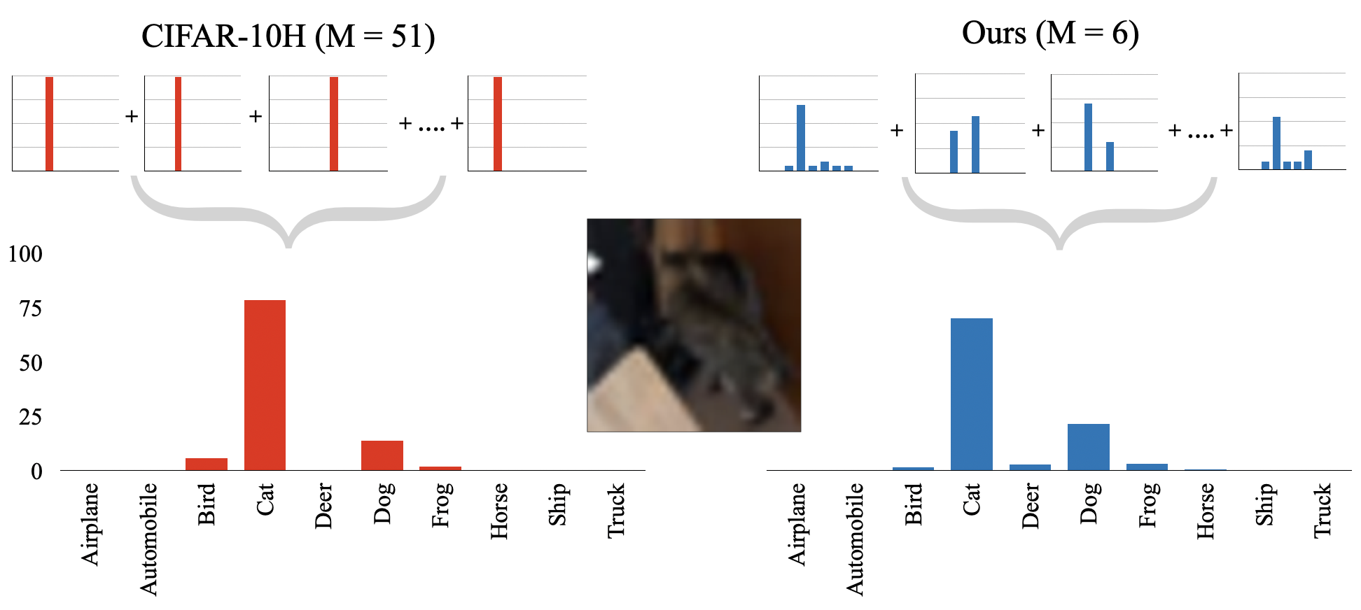
Figure 1: Unlike CIFAR-10H, we enable each annotator to express their uncertainty over image identity, enabling us to converge to richer labels faster: $M=51$ annotators for (Peterson et al. 2019) vs. $M=6$ annotators for ours.

2 Related Work

Training on soft instead of hard labels can improve robustness and generalization (Pereyra et al. 2017; Müller, Kornblith, and Hinton 2019). Soft labels have been constructed using smoothing mechanisms (Szegedy et al. 2016), auxiliary teacher networks as in knowledge distillation (Hinton et al. 2015; Gou et al. 2021), and aggregate human annotations (Sharmanska et al. 2016; Peterson et al. 2019; Recht et al. 2019; Uma et al. 2020; Gordon et al. 2021, 2022; Uma, Almanea, and Poesio 2022; Koller, Kauermann, and Zhu 2022). While the first two methods have led to significant advances in model performance, hand-crafted or learned soft labels often rely on hard labels, which tend to be impoverished representations of human precepts over datapoints. We therefore focus on the third approach, learning with soft labels derived from human annotations.

For image data, Peterson et al. (2019) construct soft labels – but do so by aggregating annotators’ hard labels for CIFAR-10 – and significantly improve classifier robustness. Uma et al. (2020) and Uma, Almanea, and Poesio (2022) extend aggregation-based soft labels to domains beyond image classification and study the incorporation of other forms of “softness,” such as temperature scaling, to enhance performance. Other works also primarily focus on aggregating hard labels from individual annotators, which have since been used for several applications, from benchmarking the reliability of foundation models (Tran et al. 2022), to informing human-machine teaming (Babbar, Bhatt, and Weller 2022; Straitouri et al. 2022), and expanding the empirical understanding of the impact of labels on performance (Wei et al. 2022; Schmarje et al. 2022). While these labels are very valuable for the community, they are often touted as representing human “label uncertainty” (Tran et al. 2022). Although such labels do capture some form of uncertainty, the picture is incomplete in only covering ambiguity across humans, and does not capture each individual’s uncertainty. Several excellent works have looked at collecting annotator confidence to address this limitation; however, in such cases, uncertainty is expressed over only the most probable label or in binary classification settings (Branson et al. 2010; Nguyen, Valizadegan, and Hauskrecht 2014; Song et al. 2018; Beyer et al. 2020; Steyvers et al. 2022). In contrast, we believe we are the first to train using rich soft labels elicited directly from annotators by requesting probabilistic judgments per annotator over multiple classes.

There is a plethora of existing works on eliciting uncertainty judgements about outcomes (O’Hagan et al. 2006; Nguyen, Valizadegan, and Hauskrecht 2014; Firman et al. 2018; Bhatt et al. 2021; Steyvers et al. 2022; Vodrahalli, Gerstenberg, and Zou 2022); however, none explicitly considers using uncertainty estimates to craft a soft label over multiple categories for training. The crowdsourcing literature has looked into the efficiency of collecting additional information from annotators (Chung et al. 2019; Méndez et al. 2022). We explicitly ask annotators to provide probabilistic judgments about labels for images, and focus our comparison not just on obtaining a soft label with fewer annotators than (Peterson et al. 2019) but also directly using our labels to confer improved machine performance.

3 Problem Setting

We focus on the $K$-way classification setting. We assume we have a dataset of $N$ images $\{x_{1},x_{2},....,x_{N}\}$ and an associated set of $N$ labels $\{y_{1},y_{2},....,y_{N}\}$, where $y_{i}$ is a vector in $[0,1]^{K}$ representing a distribution over $K$ labels. When the label is the traditional one-hot vector $y_{i}\in\{0,1\}^{K}\subseteq[0,1]^{K}$, we call this a hard label. Each image’s ordinal label may have been decided on by a single annotator (Passonneau and Carpenter 2014), or a majority vote of multiple annotators (Sheng et al. 2017). In our framework, this label distribution $P(y_{n}|x_{n})$ has all mass placed on a single class:

$$P_{\text{hard}}(y_{n}=k|x_{n})=\mathds{1}[y_{n}=k],$$

where $\mathds{1}[y_{n}=k]$ is an indicator variable of whether class $k$ has been assigned or not by a single annotator. However, this approach does not allow for the representation of annotator disagreements. As a result, others consider eliciting a single ordinal label from each of $M$ annotators, $y_{n}^{m}\in\{0,1\}^{K}$ (Peterson et al. 2019; Uma et al. 2020). This results in a distribution over labels:

$$P_{\text{multi}}(y_{n}=k|x_{n})=\frac{1}{M}\sum_{m=1}^{M}\mathds{1}[y_{n}^{m}=k].$$

The result is a soft label where $y_{n}\in[0,1]^{K}$. These labels can also be smoothed via softmax. Yet, in existing frameworks, each annotator does not have the power to express their distribution over labels. We therefore consider the case where we elicit $P(y_{n}|x_{n})$ directly from a single annotator. Here, each annotator specifies $p_{k}^{m}$, their own personal probability distribution $P_{m}$ over the labels. This allows us to aggregate all $M$ annotators’ probability distributions to form an aggregate label distribution as follows:

$$P_{\text{ours}}(y_{n}=k|x_{n})=\frac{1}{M}\sum_{m=1}^{M}p_{k}^{m},$$

where $p_{k}^{m}\in[0,1]$ that the label $y_{n}=k$, assigned by annotator $m$. We enforce the result is a valid probability distribution with $\sum_{k=1}^{K}p_{k}^{i}=1$. This framing recovers a single hard label if $M=1$ and the annotator places all their mass on one label. We recover the soft label from (Peterson et al. 2019) if all $M$ annotators place all mass on one label.

Lastly, we consider the case where we do not have complete access to all $K$ (or $K-1$, by virtue of the sum-to-one constraint of valid probability distributions) $p_{k}^{m}$ per annotator. In practice, an annotator may only specify their confidence over the top two most likely labels, or perhaps indicate some subset of the $K$ labels which are likely to have zero probability given the image. Therefore, the annotator only provides $K^{\prime}$ probability estimates where $K^{\prime}<K-1$. In this case, we need some method which distributes the leftover probability mass over the remaining $K-K^{\prime}-1$ labels. We refer to “completing” these under-specified distributions as the problem of re-distribution.

To handle re-distribution, we define a function $r$ which takes as input any elicited probabilities from the annotator, and outputs a length $K$ vector $\hat{p}_{m}$, representing the “completed” set of $K$ probabilities over the label space (where $\sum_{k=1}^{K}\hat{p}_{k}^{m}=1$). We then let:

$$P_{m}(y_{n}=k|x_{n})=r(\{p_{j}^{m}\}_{j=1}^{K^{\prime}})_{k}=\hat{p}_{m}^{k}.$$

We consider various designs for $r$ in Sec. 4.2. The resulting distributions can then be aggregated to yield a single distribution per image. We highlight in Fig. 1 the differences between eliciting label distributions which place all mass on a single class (CIFAR-10H) versus the soft labels we elicit and aggregate here.

4 Eliciting Soft Labels from Annotators

We now discuss how we collect our dataset, CIFAR-10S. To elicit soft labels from each annotator, we request:

1. The most probable label, with an associated probability

2. Optionally the second most probable label, with an associated probability

3. Any labels which the image is definitely not

The most probable and second most probable labels are selected via a radio button, whereas the selection of “definitely not” possible labels is marked through a checkbox to allow annotators to select multiple labels. Probabilities are entered in a text box and asked to be between $0$ and $100$. We do not require that probabilities sum to $100$ across the task, as we normalize after by using one of the elicitation practices of O’Hagan et al. (2006). We explore spreading any remaining mass over the labels not marked as impossible.

As we observe that an overwhelming proportion of CIFAR-10H images have mass on only two labels ($\approx$77.2%), we ask participants to specify only the top two most probable labels and any that are definitely not possible.

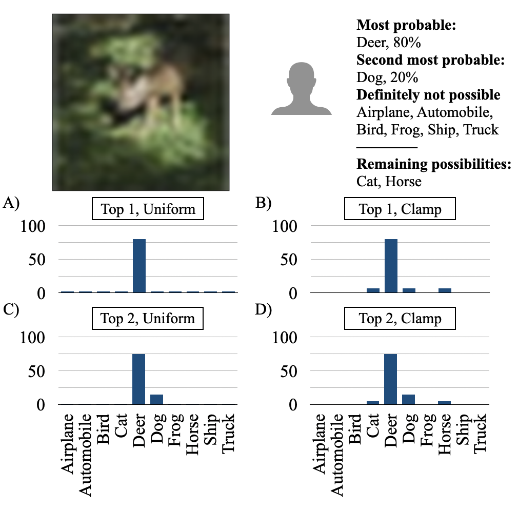
Figure 2: Depiction of constructed label varieties from the information elicited from a single annotator. Label type is depicted above the associated distribution. Note, possible labels are inferred by exclusions.

We additionally request annotators consider how other annotators, specifically “100 crowdsourced workers,” may respond. Encouraging annotators to consider a third-person perspective is reminiscent of Bayesian Truth Serum (Prelec 2004) has been shown to encourage more representative responses (Chung et al. 2019; Oakley and O’Hagan 2010). Our interface is depicted in the Appendix.

4.1 Setup

We recruited $N=248$ participants on Prolific (Palan and Schitter 2018). Participants were recruited from the United States and required to speak English as a first-language. We identified 886 images with the highest entropy (entropy $\geq$ 0.25) from CIFAR-10H (Battleday, Peterson, and Griffiths 2020; Peterson et al. 2019) to best validate the efficacy of our approach on the “hardest,” and arguably most interesting cases. Battleday, Peterson, and Griffiths (2020) found that only around 30% of the images had high inter-annotator disagreements. However, we included three images with low entropy (entropy $\leq$ 0.1) under CIFAR-10H within each batch to ensure a sufficient diversity of ambiguity was shown to each participant.

We follow Battleday, Peterson, and Griffiths (2020) in up-sampling each image to a resolution of 160x160 using Lanczos-upsampling. While this reduces the ambiguity in the traditionally low-resolution CIFAR-10 images, we aim to benchmark our method against (Peterson et al. 2019) as closely as possible and hence follow their transformation.

Each participant sees a batch of $27$ images, where two images are repeated as checks for attention and consistency. The order of labels and images was shuffled across participants. To align with local regulations, annotators are paid a base rate of $\$8$/hr with a possible bonus up to a rate of $9/hr.

We exclude any participant who did any of the following more than twice: (i) specified a probability outside of the range requested, 0 to 100; (ii) expressed that their own most probable or second most probable labels were also definitely not possible; or (iii) failed to specify any probability for their most probable label. For participants who made such errors only once, we only rule out those who provided low-quality responses by excluding those who had an accuracy against the CIFAR-10 hard labels less than 75%, the threshold used in (Battleday, Peterson, and Griffiths 2020). Our 75% accuracy exclusion threshold is only applied for annotators who made one of the above errors. We never exclude by accuracy alone in an effort to maintain diversity of percepts collected, as accuracy assumes CIFAR-10 labels are ground truth.

4.2 Constructing Soft Labels

Our elicitation yields multiple pieces of information (first and second most probable labels with specified probabilities, and labels which are deemed to have zero probability) which we can use – or ignore – when forming a soft label. We explore several varieties of soft label constructions.

How to Redistribute Extra Mass?

A central question in our elicitation scheme is how to distribute any mass which is left unspecified; for instance, if an annotator marks “truck” as the most probable class with probability 70% and “automobile” as the second most probable class at 20% likely, there is 10% of mass remaining that conceivably could be spread onto other classes. We consider two forms of redistribution in this work: 1) uniform redistribution whereby the remaining mass is spread equally over the remaining classes, or 2) clamp which uses the “definitely not” elicitation to spread the remaining mass equally over only those classes which the annotator did not specify as zero probability.

If an annotator specifies 100% of the mass over the top one or two labels but only selects a subset of the remaining labels as definitely not possible, then we posit that the annotator views the unselected classes not having zero probability. Thus, we maintain a small portion of mass $\gamma$ to be spread over the remaining classes. $\gamma$ is selected via a held-out set, as discussed in Section 5.1. We do not apply this procedure in the uniform redistribution setting, as there we assume no access to the “definitely not” information.

Label Varieties

We have $2$ x $2$ possible soft label construction methods: {most probable only, most probable and second most probable} x {redistribute uniformly, redistribute via clamp}. We use the notation T1 to specify if only the most probable class and its associated probability is used, and T2 if we include information about both the most probable and second most probable categories. We also refer to the redistribution approaches as “clamp” or “unif” following the definitions above. The label that uses all elicited information is T2 Clamp, which is the label set we refer to as CIFAR-10S. All soft labels, regardless of variety, are normalized to sum to one. Examples of constructed labels from a single annotators’ response are shown in Fig. 2.

4.3 Comparing CIFAR-10H and CIFAR-10S Label Properties

We compare the structure of our elicited labels in CIFAR-10S to CIFAR-10H labels (Peterson et al. 2019; Battleday, Peterson, and Griffiths 2020). The elicitation of CIFAR-10H is lossy because annotators may be less than $100\%$ sure about the hard label they are asked to provide. Consider if every annotator is $51\%$ sure an image is class $k$ and $49\%$ sure it is class $\ell$, then they will only provide class $k$ in the elicitation of Peterson et al. (2019). For our setting, annotators can express their label probabilities directly.

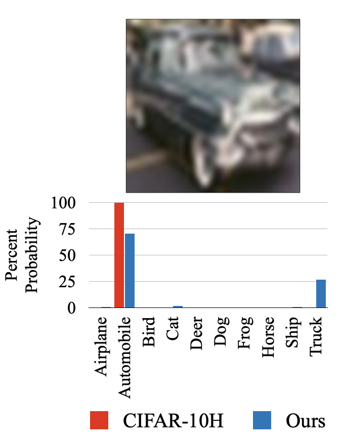
Figure 3: Our soft variant of a CIFAR-10H hard label captures inter-class similarities (i.e., trucks and automobiles).

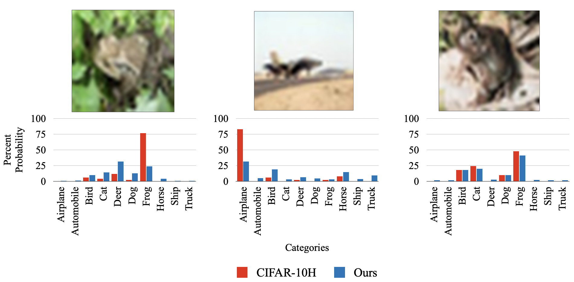
Figure 4: Comparison of our elicited labels against CIFAR-10H. From left to right: the images depict two examples with high Wasserstein distance between labels; then one example where we recover similarly rich, high entropy labels from 8.5x fewer annotators. The CIFAR-10 labels for these images are frog, airplane, and frog, respectively. Images depict what annotators actually saw; i.e., upsampling is applied following Battleday, Peterson, and Griffiths (2020).

While CIFAR-10H labels may have nearly all mass on a single class, our elicitation yields labels which have mass spread across more classes. This not only captures some of the inherent ambiguity in an image, but has the potential to provide information about the inter-class similarity structure. For example, our annotators place mass jointly over “automobiles” and the similar “truck” category, whereas a CIFAR-10H label may have all mass on the “automobile” category; see Fig. 3. We highlight additional examples of label differences in the Appendix.

Figure 5: Amount of probability placed on the most probable label and the number of “possible” labels (i.e., all those which are not selected as “Definitely Not” possible) in the T2 Clamp soft labels formed from CIFAR-10S annotators tracks CIFAR-10H label entropy (high = red, low = blue).

While our elicitation scheme yields fundamentally different labels for some images, we find our method produces remarkably similar labels to those of CIFAR-10H. Specifically, when considering T2 Clamp, the entropy of our labels has a Pearson’s $r$ correlation coefficient of 0.596, and an average Wasserstein distance of 0.028 to CIFAR-10H. This is encouraging, as we are able to recover much of the richness of CIFAR-10H labels and more from approximately 8.5x fewer annotators (an average of $M=51$ per image vs. approximately $6$ in our dataset). We depict this in Fig. 4. The amount of probability mass placed on the most probable category and the number of “impossible” labels track the CIFAR-10H label entropy (see Fig 5), which suggests that our labeling interface does yield sensible soft labels for clearer (low entropy) images.

	Label Type	CE	Calibration	FGSM Loss
CIFAR-10H	Hard Labels	2.026$\pm$0.18	0.277$\pm$0.01	15.455$\pm$7.5
	Random Labels	1.770$\pm$0.16	0.226$\pm$0.02	13.476$\pm$1.39
	Uniform Labels	1.599$\pm$0.13	0.203$\pm$0.02	10.199$\pm$3.82
	CIFAR-10H	1.325$\pm$0.07	0.201$\pm$0.01	8.750$\pm$1.80
	Ours (T2, Clamp)	1.369$\pm$0.07	0.203$\pm$0.01	8.872$\pm$1.63
CIFAR-10S	Hard Labels	4.460$\pm$0.49	0.425$\pm$0.09	15.782$\pm$4.67
	Random Labels	3.093$\pm$0.53	0.353$\pm$0.05	10.697$\pm$4.14
	Uniform Labels	2.923$\pm$0.26	0.311$\pm$0.06	11.768$\pm$5.18
	CIFAR-10H	2.558$\pm$0.16	0.313$\pm$0.03	8.416$\pm$1.64
	Ours (T2, Clamp)	2.591$\pm$0.19	0.324$\pm$0.02	9.116$\pm$1.63

Table 1: Comparing performance when training on labels aggregated from humans’ annotations ($M=51$ of CIFAR-10H annotators, $M=6$ of ours). Our soft labels here utilize all elicited information (i.e., T2 Clamp). Different labels are considered over $900$ examples. Performance is evaluated over $3000$ heldout CIFAR-10H labels (top) and $100$ heldout labels from our collection (the T2 Clamp variant of CIFAR-10S, bottom). 95% confidence intervals are included. 5 seeds are run each for three models (ResNet-34A, ResNet-50, VGG-11) and averaged. Bold indicates best performance (lower is better for all metrics).

Takeaways

Our elicitation approach enables annotators to express their distribution over image labels, approximating and expanding on the richness of CIFAR-10H from far fewer annotators. Even in cases where annotators may agree on the most likely image label, our approach – which enables annotators to express their probability judgments over possible other categories – yields labels which potentially better represent the distribution over labels.

	Label Type	CE	Calibration	FGSM Loss
10H	CIFAR-10H	1.293$\pm$0.08	0.194$\pm$0.01	8.577$\pm$1.91
	Ours (T2, Clamp)	1.281$\pm$0.06	0.184$\pm$0.01	8.406$\pm$1.75
10S	CIFAR-10H	2.459$\pm$0.21	0.311$\pm$0.02	8.334$\pm$1.75
	Ours (T2, Clamp)	2.355$\pm$0.14	0.297$\pm$0.03	8.405$\pm$1.59

Table 2: Training with de-aggregated labels; on each batch, a single humans’ label is used as supervisory signal from a pool of $M$ humans ($M=51$ CIFAR-10H; $M=6$ ours).

5 Evaluating the Efficacy and Efficiency of Learning with Per-Annotator Soft Labels

We investigate how learning over our elicited soft labels compares against learning over labels drawn from CIFAR-10H. CIFAR-10H labels have previously been shown to confer generalization benefits over several other soft labeling approaches, such as class-level confusion-based smoothing and knowledge distillation (Peterson et al. 2019). We focus on performance when constructing labels from sub-samples of annotators. This enables us to investigate the annotator efficiency of our soft label elicitation. Additionally, we study the impact of constructing labels from subsets of elicited data. We also consider performance differences in light of the total time elicitation takes.

5.1 Setup

Setup

Our model and training procedures follow Uma et al. (2020), as they explore learning with CIFAR-10H labels and explicate a clear, standardized learning procedure. We employ the same ResNet-34A (He et al. 2016) with the same weight decay (1e-4) and learning rate scheduling: we start with a learning rate of $0.1$ and drop by a factor of 1e-4 after epoch $50$ and again at $55$. To compare the utility of our soft labels during learning across a range of settings, we also consider two additional architectures not included in Uma et al. (2020): VGG-11 (Simonyan and Zisserman 2014) and ResNet-50 (He et al. 2015). Starting learning rates are selected using a validation set of CIFAR-10 ($0.1$ for VGG-11 and $0.4$ for ResNet-50 from $\{0.001,0.01,0.1,0.2,0.3,0.4,0.5\}$. All models are trained from scratch for a total of $65$ epochs and optimize a cross-entropy objective. Experiments are run over $5$ seeds, unless otherwise noted. A redistribution factor of $\gamma=0.1$ is used to spread extra mass, selected via the same validation procedure from $\{0.0,0.01,0.05,0.1,0.2,0.3,0.4\}$.

We follow the same 70/30 split used in (Uma et al. 2020). However, as we have fewer CIFAR-10S labels than CIFAR-10H, to ensure a fair comparison, we consider just training on the CIFAR-10H labels for which we have our soft label versions. Note, we always hold out $100$ of our labels to ensure we can evaluate against some variant of our soft labels. Thus, we are considering the variation in performance conferred by changing 900 labels. For the remaining examples in the 6,100 – we use a hard version, i.e., the original CIFAR-10 label.

		M=2			M=1
	Labels	CE	Calib	FGSM	CE	Calib	FGSM
10H	10H	1.71$\pm$0.15	0.25$\pm$0.02	14.16$\pm$0.67	2.17$\pm$0.11	0.29$\pm$0.01	19.20$\pm$0.86
	Ours	1.49$\pm$0.08	0.22$\pm$0.01	11.57$\pm$0.44	1.58$\pm$0.08	0.23$\pm$0.01	12.57$\pm$1.29
10S	10H	3.37$\pm$0.42	0.34$\pm$0.08	13.13$\pm$0.7	4.49$\pm$0.31	0.45$\pm$0.05	17.85$\pm$0.68
	Ours	2.88$\pm$0.17	0.36$\pm$0.04	11.39$\pm$0.59	2.90$\pm$0.31	0.38$\pm$0.06	12.13$\pm$1.31

Table 3: Investigating model performance when fewer $M$ annotators are assumed to provide labels. Training labels are sampled per batch instead from a pool of $M=2$ or $M=1$ annotators.

Evaluation Data

Selection of data used to evaluate models is important to faithfully benchmark performance; however, typical evaluation datasets like the CIFAR-10 test set are rife with annotation errors (Northcutt, Athalye, and Mueller 2021) and as discussed throughout this work, if hard labeled, do not adequately capture human uncertainty. We instead use heldout aggregate soft labels from CIFAR-10H and our CIFAR-10S as test sets. While humans are of course not always correct in their annotations themselves, nor calibrated in their confidence, these labels serve to better measure whether models handle example ambiguity. Note, as the labels we collect are enriched to be more ambiguous (see Section 4.1), at present, CIFAR-10S could be an inherently challenging evaluation set.

Metrics

No single metric captures all the qualities we wish to obtain in a trustworthy model (Thomas and Uminsky 2022). We therefore consider a suite of metrics, focused on generalization, calibration, and robustness.

1. Generalization: we measure generalization using Cross Entropy (CE) over the soft labels, which allows us to capture whether the models’ full distribution over the $K$ categories is sensible: $\frac{1}{N}\sum_{1}^{N}\sum_{1}^{K}P_{\text{eval}}(y_{n}=k|x_{n})\log(f_{\theta}(x_{n})_{k})$, where $P_{\text{eval}}$ is the label distribution derived from the human soft labels, drawn from either CIFAR-10H or our CIFAR-10S collection, and $f_{\theta}(x_{n})_{k}$ is the probability assigned by our model $f$ (parameterized by $\theta$) to the $k$-th category on the $n$-th input.

2. Calibration: model calibration is scored using the RMSE adaptive-binning method used by Hendrycks et al. (2022) to measure whether models’ predictive distributions match their “correctness”. Here, “correct” is based on: $\operatorname*{arg\,max}_{k\in\{1,...,K\}}P_{\text{eval}}(y_{n}=k|x_{n})$.

3. Robustness: loss after a Fast Gradient Sign Method (FGSM) attack is used to measure models’ robustness to an adversarial attack (Goodfellow, Shlens, and Szegedy 2015). Attack strength is run at an $\ell_{\infty}=4$ bound following Peterson et al. (2019).

Annotation Time

We include estimated total annotation time for each labeling scheme. We let total annotation time equal $M\times t_{\text{per}}$, where $M$ is the number of annotators being aggregated per image and $t_{\text{per}}$ is the estimated time taken per annotator to obtain that label type. Our elicitation takes a median of $32$ seconds for annotators to provide the most probable label with an associated probability, optionally the second most probable label with a probability, and any label which are definitely not perceived as the image category. This entails five different inputs from an annotator. As we do not have access to the time taken for each input, we assume that each takes roughly the same amount of time. We assign an estimated $6.4$ seconds to the elicitation time per input. We compute the median amount of time taken for CIFAR-10H annotators over the same images using their released raw annotation data, which comes to approximately $t_{\text{per}}=1.8$ seconds per image. Note, this value does not account for the training phase that Battleday, Peterson, and Griffiths (2020) used per annotator, which could have increased total costs. However, even so, we acknowledge that comparatively high time costs of our elicitation scheme are a signification limitation of our work at present; designing more efficient soft label elicitation is a promising direction for future work.

5.2 Learning with Soft Labels

We first compare our naively aggregated per-annotator soft labels using all information elicited from annotators (i.e., T2, Clamp) against the complete aggregate labels from CIFAR-10H, i.e., labels formed from all of their approximately 51 labelers. As noted in Section 5.1, we use heldout CIFAR-10H and CIFAR-10S labels as a proxy for “test truth” when evaluating. We benchmark performance against training on conventional CIFAR-10 hard labels, as well as training on random and uniform labels. A discussion of label smoothing is included in the Appendix.

As shown in Table 1, we find that, even from approximately 8.5x fewer annotators than CIFAR-10H, our per-annotator soft labels endow the learned classifier with performance comparable to that obtained by using the CIFAR-10H labels.

However, prior work has indicated that training on separated, de-aggregated labels could yield better performance when there are few, noisy annotators (Wei et al. 2022). Peterson et al. (2019) similarly found learning on de-aggregated labels was sometimes advantageous, which they hypothesize is from more varied gradient information. As such, we next compare model performance when trained on de-aggregated labels. That is, at each batch, a single annotator’s label (from the pool of $M$) is sampled for use as the supervisory signal. In this setting, we see in Table 2 that our CIFAR-10S labels confer substantial benefits over CIFAR-10H across nearly all metrics, despite having $8.5$x fewer annotators. As models trained on de-aggregated labels enjoyed better performance across both datasets, we use the de-aggregated setting for all further experiments.

In Table 3, we subsample $M=2$ of the annotators in CIFAR-10H from which to construct a label per batch, and compare the utility of learning with said labels against a similarly sub-sampled version over two of our per-annotators’ soft labels per image. We find that our labels provide a substantial boost along nearly all metrics – and the gains of our method in the few annotator setting become even more apparent when considering access to only $M=1$ human. While this is expected, as a single CIFAR-10H labeler is simply a hard label, we demonstrate that if one has access to only a single annotator, our label method provides the best training signal.

We depict a full comparison of performance when varying the number of annotators we are aggregating over in Fig. 6. Across most metrics and evaluation sets, our method is significantly more annotator efficient. We recognize, however, that total annotation time (accounting for the time spent per annotator) is also a practical concern. We visualize the same performance relationship with total estimated annotation time ($M*t_{\text{per}}$ ) in the Appendix. On this cost basis, it is not clear whether our labels are advantageous.

It is possible then that we could get by with less information elicited per annotator. We explore how model performance varies as a function of the various label types that could be construed from our elicitation (see Fig 2). We do find in Table 4 that while learning with all elicited information (T2, Clamp) yields the most consistently appealing performance, we could achieve relatively good calibration and robustness in particular from less information (such as not requiring the clamp, or not eliciting probabilistic information about the second most probable label if using a Clamp) – though more work is needed to tease apart the benefits of each elicited bit of information towards supporting a models’ predictive power.

Takeaways

Eliciting and learning with individuals’ soft labels – from a few annotators – results in a classifier that achieve better performance and robustness compared to the results of Peterson et al. (2019) who used many more annotators, particularly when de-aggegated during training. This highlights that collecting categorical soft labels can be beneficial. While our method offers consistent advantages in the few-annotator regime, the benefits of eliciting per-annotator soft labels versus many annotators’ hard labels is not clear when accounting for total annotation time.

	Label Type	Time	CE	Calibration	FGSM Loss
10H	T1, Unif	76.8s	1.320$\pm$0.08	0.187$\pm$0.01	8.647$\pm$1.72
	T1, Clamp	115.2s	1.299$\pm$0.06	0.19$\pm$0.01	8.385$\pm$1.55
	T2, Unif	153.6s	1.287$\pm$0.10	0.180$\pm$0.02	8.345$\pm$1.63
	T2, Clamp	192.0s	1.281$\pm$0.06	0.184$\pm$0.01	8.406$\pm$1.75
10S	T1, Unif	76.8s	2.512$\pm$0.12	0.317$\pm$0.04	9.029$\pm$1.7
	T1, Clamp	115.2s	2.501$\pm$0.18	0.306$\pm$0.03	8.590$\pm$1.42
	T2, Unif	153.6s	2.437$\pm$0.16	0.293$\pm$0.04	8.605$\pm$1.59
	T2, Clamp	192.0s	2.355$\pm$0.14	0.297$\pm$0.03	8.405$\pm$1.59

Table 4: Training models over labels constructed from subsets of the human knowledge we elicit. $M=6$ humans’ labels are used to form the pool sampled. Time depicts the estimated elicitation time (over $M=6$ annotators) for a given example.

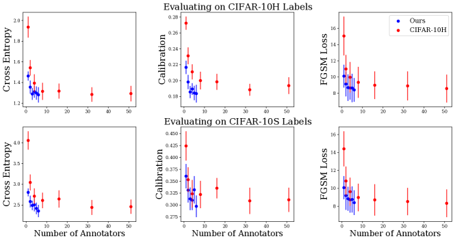
Figure 6: Comparison of learner performance based on number of annotators used to create the training labels. Red dots depict performance when aggregating $M$ CIFAR-10H annotators for $M\in\{1,2,4,8,16,32,\text{all}\}$. Blue dots indicate CIFAR-10S T2 Clamp soft labels, constructed from varying $M\in\{1,2,3,4,5,6\}$. Dots represent performance averaged over $15$ seeds ($5$ run per architecture type).

5.3 Simulating Annotations without Elicited Uncertainty

We have so far shown that our soft label approach yields comparable performance and even outperforms models trained with CIFAR-10H labels along most metrics in the few annotator regime. This holds across several varieties of soft labels that can be formed from our labels. However, it is unclear the extent to which eliciting annotator probability estimates is beneficial.

We address this question by training a model on labels which simulate the setting where an annotator could only select the two most probable labels (“Select Top 2 Only”). In this scenario, we assume that we do not have access to annotators’ relative likelihood weightings amongst those two classes; therefore, we spread mass uniformly over the top two selected. We compare this against our labels which do allow annotators to specify relative probabilities. We see in Table 5 that relative uncertainty information does allow the construction of more effective labels for a learner.

	Label Type	Time	CE	Calibration	FGSM Loss
10H	Select Top 2 Only	76.8s	1.300$\pm$0.06	0.180$\pm$0.01	8.639$\pm$1.46
	Top 2 With Prob (Unif)	153.6s	1.287$\pm$0.10	0.180$\pm$0.02	8.345$\pm$1.63
	Top 2 With Prob (Clamp)	192.0s	1.281$\pm$0.06	0.184$\pm$0.01	8.406$\pm$1.75
10S	Select Top 2 Only	76.8s	2.448$\pm$0.15	0.313$\pm$0.02	8.797$\pm$1.25
	Top 2 With Prob (Unif)	153.6s	2.437$\pm$0.16	0.293$\pm$0.04	8.605$\pm$1.59
	Top 2 With Prob (Clamp)	192.0s	2.355$\pm$0.14	0.297$\pm$0.03	8.405$\pm$1.59

Table 5: Training with ablated annotator uncertainty over de-aggregated labels drawn from the pool of $M=6$ annotators. Here, “Select Top 2 Only” places equal mass on the labels selected as most probable and second most probable by each annotator.

Takeaways

Eliciting probability information, rather than simply selecting the most probable classes, provides useful learning signals to improve generalization and robustness.

6 Discussion

Fewer Annotators Needed if Eliciting Soft Labels

We demonstrate that constructing training labels from per-annotator soft labels allows practitioners to use significantly fewer labelers and still enjoy the benefits of improved model generalization, bolstered robustness, and better calibration found when aggregating many annotators’ hard labels (Peterson et al. 2019). While online crowdsourcing platforms like Prolific (Palan and Schitter 2018) and Amazon Mechanical Turk (MTurk) enable researchers to rapidly scale experiments to many annotators, it may be challenging to recruit large numbers of annotators in domains that require expertise like medicine or criminal justice. Our elicitation approach serves to lower the barrier for efficient in-house data annotation: when it is hard to recruit many annotators, our approach to eliciting soft labels from just a few annotators may be particularly effective. Such annotator efficiency could also be used to support rapid personalization. As an example, “teachable object recognition” is being used to enable people with visual challenges to adapt classifiers to their particular needs (Massiceti et al. 2021). In this application area, we may only have a single vision-impaired user per input, warranting the need for rich, single-annotator schemes such as the one we propose.

The Sensibility of Eliciting Annotator Probabilities

The notion of eliciting soft labels from annotators has conceptual niceties. In particular, our labeling scheme empowers annotators to express probability judgements they have in their label assignment. In a hard label setting, annotators are required to select a single label (Peterson et al. 2019); however, an annotator has no means to express if they have any ambiguity in their label, which could occur if the image is particularly noisy or there are many similar label options. While humans have been found to have biases in their probabilistic assessments of the likelihood of phenomena (Lichtenstein, Fischhoff, and Phillips 1977; Tversky and Kahneman 1996; O’Hagan et al. 2006; Sharot 2011), we do not think this is a sufficient reason to avoid eliciting probability judgments from annotators. As noted by O’Hagan et al. (2006) and O’Hagan (2019), human uncertainty can be elicited reliably as long as elicitation is rigorous. If an annotator is unsure of their decision, forcing an annotator to compress out all of this uncertainty by specifying one hard label only exacerbates, rather than solves, the challenge of capturing annotator ambiguity.

Indeed, reasoning under uncertainty is a linchpin of human cognition (Lake et al. 2017) and has been shown to be a central component of “good” decision-making (Laidlaw and Russell 2021; Bhatt et al. 2021). Careful consideration of uncertainty is of particular importance in high-stakes areas like medicine wherein diagnoses and suitable treatment plans may not be absolutely certain (Hall 2002; Shrager, Shapiro, and Hoos 2019; Platts-Mills, Nagurney, and Melnick 2020; Cox et al. 2021). Hence, annotation schemes which enable the expression of probability judgements, particularly in datasets wherein the underlying “ground truth” or the “true” label is unknown, may be sensible and desirable for improving machine safety, trustworthiness, and efficacy. Our elicitation approach takes a practical step towards this goal and offers pragmatic benefits for learning and generalization.

Hence, annotation schemes which enable the expression of probability judgements, particularly in datasets wherein the underlying “ground truth” or the “true” label is unknown, may be sensible and desirable for improving machine safety, trustworthiness, and efficacy. Our elicitation approach takes a practical step towards this goal and offers pragmatic benefits for learning and generalization.

Considerations of Ground Truth and Performance

Battleday, Peterson, and Griffiths (2020) require their annotators to be accurate with respect to CIFAR-10 labels. The average annotator accuracy of CIFAR-10H is 95%. We do not discard annotators by accuracy alone, hence our annotator accuracy is slightly lower: annotators chose the CIFAR-10 label as the top label approximately 84% of the time and include this label in their top two choices 92% of the time. We hope our dataset may be helpful for researchers studying learning from semi-noisy annotators.

While many ML tasks assume a ‘true’ label to calculate metrics like accuracy, there are settings where it is not possible or sensible to aim for a single true label agreed upon by all annotators. It is unclear what should count as “ground truth” in how we evaluate models. Our soft labels permit multiple categories to be simultaneously considered without explicit consensus, and therefore offer an alternative form of evaluation potentially well-suited for such settings.

Limitations

While our labeling methods yield conceptual benefits, and potential advantages in annotator efficiency and improved performance, we recognize that currently our approach is significantly slower to collect per annotator than hard labeling. Moreover, we have only considered a single annotation framework, and as we have seen, model performance is sensitive to the structure of the provided labels. It is therefore possible that alternative elicitation paradigms, such as those wherein annotators select more than just their inferred top 2 most probable categories or even provide soft labels graphically through a constructed histogram (Goldstein and Rothschild 2014), could yield different labels and hence impact model training. And while we did not find significant intra-annotator variability on repeat trials, it is important to consider whether annotators’ internal label distributions are stable over time (Murray, Patel, and Yee 2015). We also note that even though our elicitation framework enables us to learn effectively from fewer annotators, too few annotators could yield various biases, especially as “50%” to one annotator may not mean the same to another, and the inherent task difficulty could impact whether more annotators ought to be recruited – even if effective learning in the current study can be achieved from few annotators.

Indeed, we are cognizant that our findings are within a particular domain, image classification, over a particular dataset, the test set of CIFAR-10 (i.e., we collect annotations over $10\%$ of CIFAR-10H). Here, we have a managable number of categories to elicit information over; it is hard to imagine an annotator selecting all impossible categories if there are 100s or 1000s as may be the case in other ML datasets (Fei-Fei, Deng, and Li 2009). More work is needed to verify if our results generalize to other settings, and extend beyond the crowdsourcing space to real-world domain experts. All participants considered here are based in the United States and speak English as their first language. As discussed in (Prabhakaran, Davani, and Diaz 2021; Díaz et al. 2022), recruiting a diverse group of annotators from different backgrounds and releasing disaggregated annotator responses is valuable to ensure a broad spectrum of human experiences and world views are captured in datasets.

Using and Extending our Interface

To design more time-efficient elicitation and scale our soft label elicitation interface to other domains, we make our elicitation interface publicly available. To apply our set-up to a new problem, all one needs are: 1) a folder of the images one wishes to present to the annotator, 2) a set of labels that the annotator is allowed to select, and 3) an allocation of images to batches (e.g., a .json file). We hope the ease with which our interface can be adapted to new domains will lower the barrier of entry for others to run their own soft label data collection.

Additional Extensions

Future work can consider how the elicitation of soft labels via annotator probabilities may change over a broader set of datasets and domains, and may alter if eliciting across a wider spectrum of annotator backgrounds, where some may be assumed to have access to “privileged information” based on their experiences which are worthy to model (Sharmanska et al. 2016). And in light of the time costs of our elicitation, we see promise in developing active methods to identify which images may benefit most from being queried via our rich elicitation scheme. We encourage researchers and designers to create more time-efficient schemes to elicit rich annotator probability or uncertainty measures towards constructing good soft labels.

We have only considered simple naive averaging to aggregate annotations; future work could draw on the expansive literature concerning aggregation (Dawid and Skene 1979; Smyth et al. 1994; Levin and Nalebuff 1995; Whitehill et al. 2009; Ho, Frongillo, and Chen 2016; Sharmanska et al. 2016; Augustin et al. 2017; Zhang and Wu 2018; Wang, Liu, and Chen 2021; Wei et al. 2022; Collier et al. 2022) to develop better schemes which may take into account differential annotator characteristics such as trustworthiness and expertise. We encourage researchers to evaluate the efficacy of our constructed soft labels in other learning paradigms, such as weakly supervised learning (Arazo et al. 2019; Wei et al. 2022), online learning (Chen et al. 2022), or curriculum learning (Liu et al. 2017), and as human-grounded priors in Bayesian neural network settings (Fortuin 2022).

7 Conclusion

In this work, we have shown the benefits of eliciting and aggregating per-annotator soft labels over aggregating hard labels on the CIFAR-10 dataset (Peterson et al. 2019). The benefits we observe include: improved model generalization, calibration, and robustness from fewer total annotators; and richness in the learning signal which enables improved calibration. We release the code for our elicitation interface and our collected soft label dataset as CIFAR-10S. We hope that our work encourages others to explore the benefits of eliciting soft labels from annotators.

Appendix

This Appendix includes:

1. Our elicitation interface shown to recruited participants in Fig. 7.

2. Additional elicited label distributions in Figs. 8 and 9.

3. A comparison against classical label smoothing in Table 6, with a discussion of the results in the following section.

4. Performance as a factor of estimated total annotation time in Fig. 10.

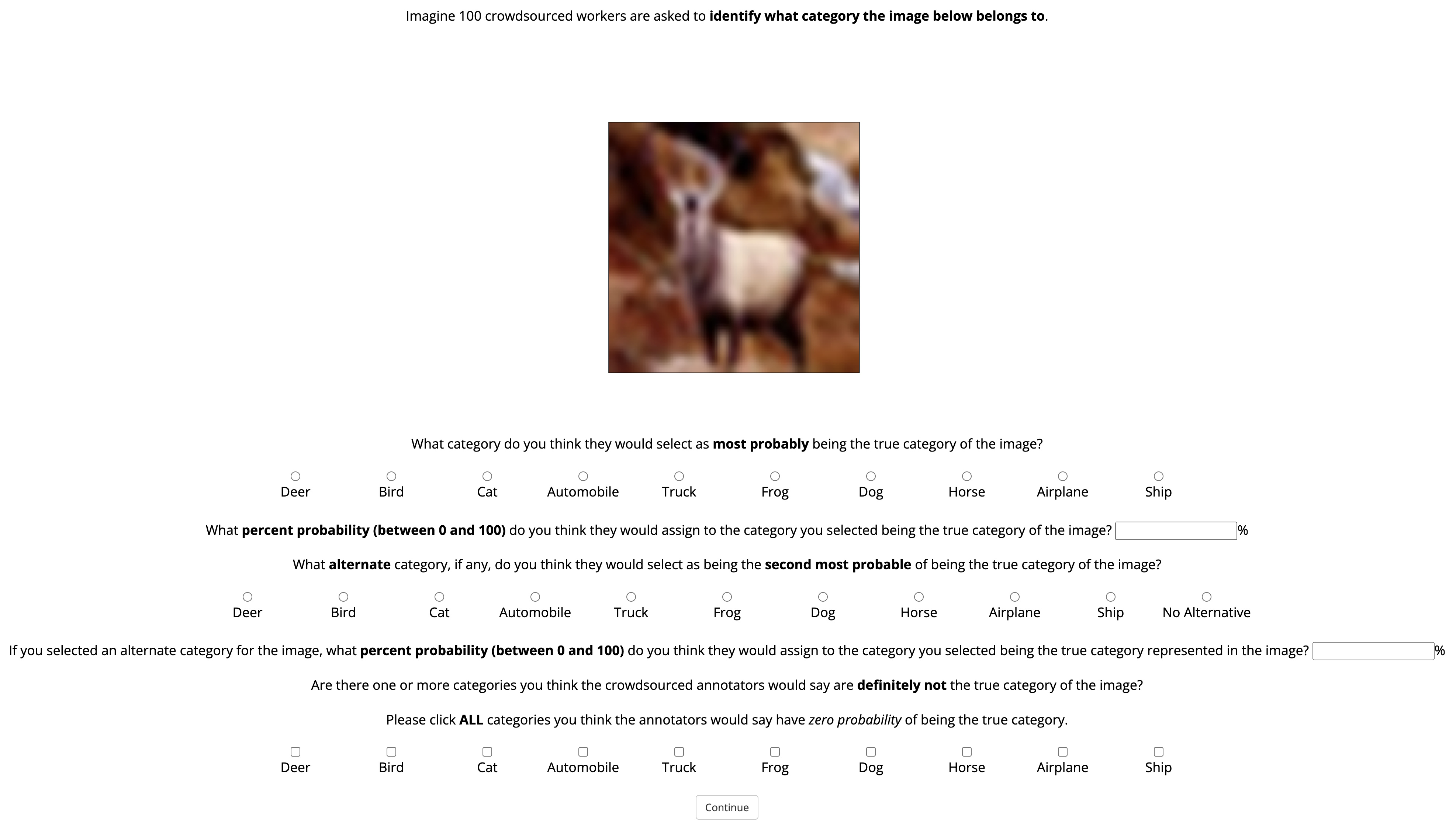
Figure 7: Depiction of our soft label elicitation interface.

	Label Type	CE	Calibration	FGSM Loss
10H	Label Smoothing	1.368$\pm$0.19	0.175$\pm$0.05	6.965$\pm$1.7
	CIFAR-10H	1.293$\pm$0.08	0.194$\pm$0.01	8.577$\pm$1.91
	Ours (T2, Clamp)	1.281$\pm$0.06	0.184$\pm$0.01	8.406$\pm$1.75
10S	Label Smoothing	2.674$\pm$0.33	0.299$\pm$0.05	9.375$\pm$3.4
	CIFAR-10H	2.459$\pm$0.21	0.311$\pm$0.02	8.334$\pm$1.75
	Ours (T2, Clamp)	2.355$\pm$0.14	0.297$\pm$0.03	8.405$\pm$1.59

Table 6: Comparing de-aggregated human-derived soft labels against label smoothing.

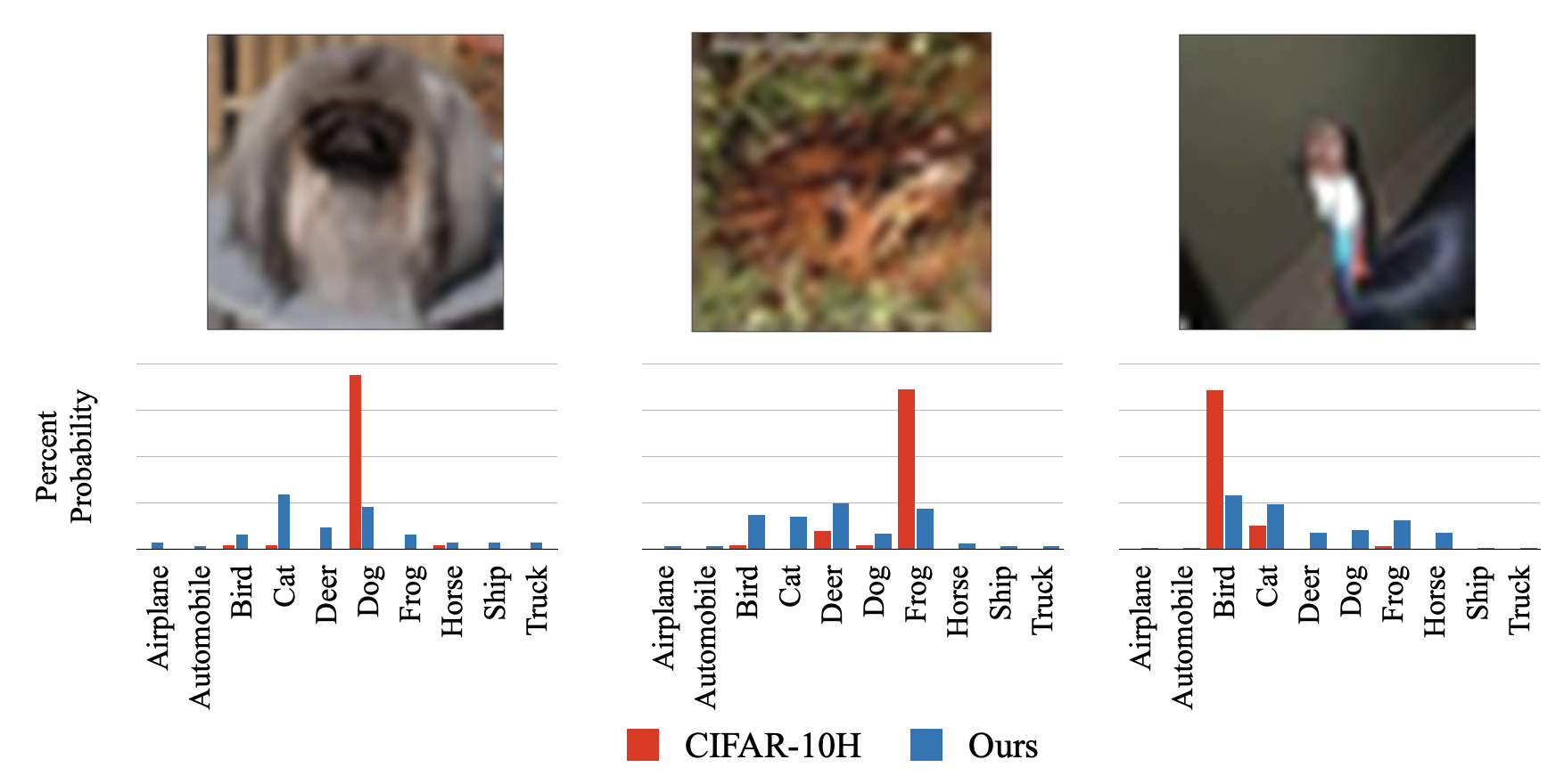
Figure 8: Top three highest Wasserstein distance examples between our CIFAR-10S labels (blue) and CIFAR-10H (red). The hard labels in CIFAR-10 are: dog, frog, and bird.

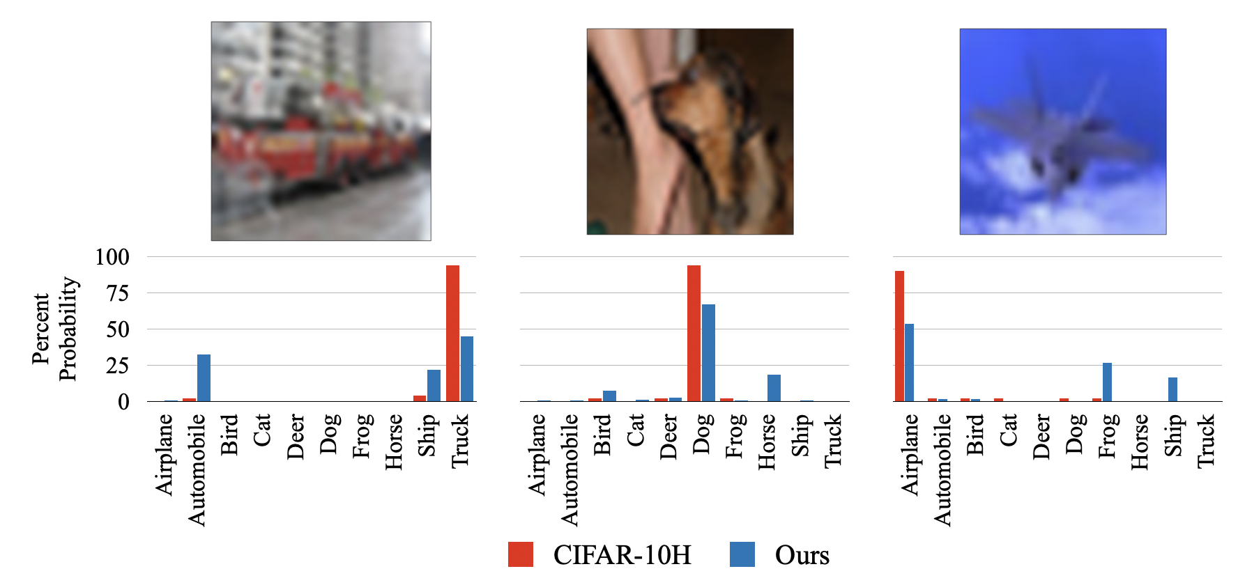
Figure 9: Additional examples demonstrating the “softening” of CIFAR-10H labels with our elicitation. The hard labels in CIFAR-10 are: truck, dog, and airplane.

Relationship to Classical Label Smoothing

When considering the value of eliciting and incorporating additional human knowledge in ML systems, one may ask why not just use traditional label smoothing (LS)?

$$y^{\text{LS}}_{n}=y^{\text{hard}}_{n}*(1-\beta)+\beta*y^{\text{smoother}}$$

$y^{\text{smoother}}$ is a uniform of length $K$ (each “probability” $=\frac{1}{K}$ (applied to all N examples), $y^{\text{hard}}_{n}$ is the conventional one-hot label, and $\alpha$ is the smoothing factor $\in[0,1]$.

We train the three models considered in Section 5.1 over labels on which LS ($\beta=0.05$) was applied. We tune $\beta$ ($\in\{0,0.0001,0.001,0.01,0.05,0.1,0.2,0.3,0.4\})$) with the same validation method discussed. We find in Table 6 that LS does outperform both CIFAR-10H and CIFAR-10S in terms of calibration and roubstness over CIFAR-10H; however, this does not hold when evaluated on CIFAR-10S. While these results do shed light on a nuance of human knowledge elicitation (alternative, automated ML approaches are powerful already); we argue that human knowledge still contributes valuable insights. Importantly, LS does not capture meaningful softness, i.e., an image most likely to be a deer has equal probability of alternatively being a dog as a ship. This lack of human-sensible alternatives may prohibit effective generalization to our richer, harder CIFAR-10S evaluation set; a result of which has been shown on other datasets (Zhang et al. 2021). Furthermore, the blanket mass spread over all $K-1$ alternatives also has been found to lead to oversimplified clusters (Müller, Kornblith, and Hinton 2019). It is worth investigating the kinds of latent spaces that result from training over our human-derived soft labels instead.

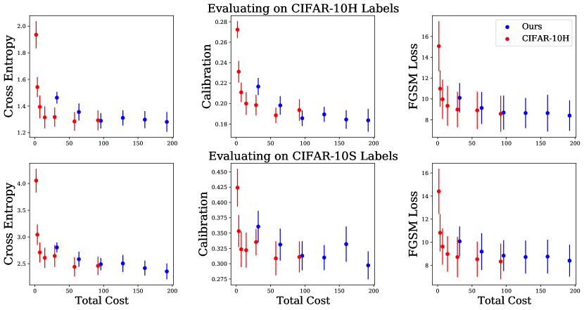
Figure 10: Comparison of learner performance as a factor of estimated total cost of elicitation ($M*t_{\text{per}}$). Red dots depict performance when aggregating $M$ CIFAR-10H annotators for $M\in\{1,2,4,8,16,32,51\}$. Blue dots indicate CIFAR-10S T2 Clamp soft labels, constructed from varying $M\in\{1,2,3,4,5,6\}$. Dots represent performance averaged over $15$ seeds ($5$ run per architecture type).

References

- Arazo et al. (2019) Arazo, E.; Ortego, D.; Albert, P.; O’Connor, N.; and McGuinness, K. 2019. Unsupervised label noise modeling and loss correction. In International conference on machine learning, 312–321. PMLR.
- Augustin et al. (2017) Augustin, A.; Venanzi, M.; Rogers, A.; and Jennings, N. R. 2017. Bayesian Aggregation of Categorical Distributions with Applications in Crowdsourcing. In IJCAI, 1411–1417.
- Babbar, Bhatt, and Weller (2022) Babbar, V.; Bhatt, U.; and Weller, A. 2022. On the Utility of Prediction Sets in Human-AI Teams. In IJCAI.