A novel technique for the measurement of the avalanche fluctuations
of a GEM stack using a gating foil

Abstract

We have developed a novel technique for the measurement of the size of avalanche fluctuations of gaseous detectors using a gating device (gating foil) prepared for the time projection chamber in the international linear collider experiment (ILD-TPC). In addition to the gating function, the gating foil is capable of controlling the average fraction of drift electrons detected after gas amplification. The signal charge width and shape (skewness) for electron–ion pairs created by a pulsed UV laser as a function of the transmission rate of the gating foil can be used to determine the relative variance of gas gain for single electrons. We present the measurement principle and the result obtained using a stack of gas electron multipliers (GEMs) operated in a gas mixture of Ar-CF₄ (3%)-isobutane (2%) at atmospheric pressure. Also discussed is the influence of the avalanche fluctuations on the spatial resolution of the ILD-TPC.

1 Introduction

Gas amplification of the electrons created by X-rays or charged particles plays an essential role in their detection with gaseous detectors. However, gain fluctuations due to avalanche statistics degrade the spatial resolution of large Time Projection Chambers (TPCs) [1, 2, 3] at long drift distances [4, 5, 6, 7, 8] as well as the energy resolution for monochromatic X-rays.

We are now developing a TPC for the central tracker of the linear collider experiment (ILD-TPC) featuring a double stack of gas electron multipliers (GEMs) [9] for its gas amplification device. The ILD-TPC is required to have a high spatial resolution of $<$$\sim$ 100 $\mu$m for high momentum charged particles along the pad row direction with a pad-row height of 5 - 7 mm [10]. The azimuthal spatial resolution ($\sigma_{\rm X}$) for stiff radial tracks at long drift distances ($z$) is given by

$$\sigma_{\rm X}^{2}=\frac{1}{N_{\rm eff}}\cdot\left(B_{0}^{2}+D^{2}\cdot z\right)$$ (1)

with

$$\frac{1}{N_{\rm eff}}\equiv\left(1+f\right)\cdot\biggl{<}\frac{1}{N_{\rm t}}\biggr{>}$$ (2)

where $B_{0}$ is a controllable constant term determined by the pad width and the amplified charge spread in the GEM stack, and $D$ denotes the transverse diffusion constant of drift electrons while $f$ is the relative variance of the avalanche fluctuations for single drift electrons, and $N_{\rm t}$, the number of drift electrons reaching the sensitive area covered by the pad row [4].

It is therefore important to make the values of $D$ and $1/N_{\rm eff}$, both determined by the choice of the chamber gas (once the pad-row height is fixed for the latter), small enough to keep the degradation of the spatial resolution acceptable at the maximum drift length of 2.35 m. We plan to use a gas mixture of Ar-CF₄ (3%)-isobutane (2%) because of its small value of $D$ ($\sim$ 30 $\mu$m/$\sqrt{{\rm cm}}$) under a drift field of 230 V/cm and an axial magnetic field of 3.5 T. An argon-based gas mixture was chosen because of its smaller $W$-value that makes $\left<1/N_{\rm t}\right>$ smaller, as compared to neon-based mixtures, for example. This merit could, however, be compromised by a larger value of $f$ for argon-based mixtures. Accordingly, we need to know the value of $f$, as well as of $\left<1/N_{\rm t}\right>$, to estimate the azimuthal spatial resolution achievable with the ILD-TPC.

The size of the avalanche fluctuations has been investigated mathematically [11] or numerically [12] and measured by many researchers with a variety of gas-amplification devices for various filling gases (see, for example, Refs. [13, 14, 15, 16, 17, 18, 19, 20, 21, 22]. A concise review before the emergence of Micromegas [23] and GEM can be found in Section 2 of Ref. [24]. However, measurements of the avalanche fluctuations in argon-based gases are scarce for GEMs, in particular for double GEM stacks, which are our current choice, and no literature is available except for our past measurement [25] for a relatively new gas mixture of Ar-CF₄ (3%)-isobutane (2%), to our knowledge. In addition, we are now using 100-$\mu$m thick non-standard GEM foils to obtain an adequate gas gain with a double GEM stack (see Section 3). We, therefore, carried out a new measurement to confirm our previous results using different techniques (see below).

The most common and straightforward way to study the avalanche fluctuations is to observe directly the gas-amplified charge spectrum for single photoelectrons created by irradiating a cathode material by an ultraviolet (UV) lamp, LED, or laser. However, this technique requires a high gas gain and/or low electronic noise, and a relatively long measurement time during which the gas density has to be kept constant. It would be much easier if the size of the avalanche fluctuations can be deduced from the signal charge distribution for a larger number of drift electrons.

We presented such a technique using laser-induced tracks (uniformly-distributed electron–ion pairs), which enabled the measurements even at low gas gains in around 10 minutes, and without any assumption on the functional form of the avalanche fluctuations [25]. Recently, we found yet another technique for the measurement of the size of avalanche fluctuations in the course of the performance evaluation of a gating device (gating foil) developed for the ILD-TPC using laser-induced tracks. In addition to the gating function, the gating foil [26] is capable of controlling the average fraction of drift electrons detected after gas amplification. The signal charge width and the shape (skewness) as function of the average signal charge controlled by the gating foil enabled us to measure the relative variance ($f$) of gas gain for single drift electrons. This technique is similar to the measurement of $f\/$ for the same double GEM stack operated in Ar-CF₄ (3%)-isobutane (2%) using an ⁵⁵Fe source and the gating foil presented in the appendix of Ref. [26].

The next section briefly summarizes the history of the applications of lasers to gaseous detectors, including the features of our present experiment. The experimental setup and the measurement principle are described respectively in Sections 3 and 4. The result is given in Section 5. Section 6 is devoted to the discussion and Section 7 concludes the paper.

2 Brief history of the application of lasers to gaseous detectors

The use of lasers for creating ion pairs in gaseous detectors has a long history. A combination of UV and visible laser beams was first used by Hurst et al. to measure the avalanche fluctuations and the Fano factor with a cylindrical counter operated in a doped chamber gas [27]. It was then found that a single UV laser could be used for the calibration of chambers with a gas doped with nickelocene [28].

Shortly after that, J. Bourotte and B. Sadoulet, and H.J. Hilke showed that UV lasers could ionize trace impurities (natural contaminants) in a chamber gas and could create straight tracks along the laser beam [29, 30]. The ionizations of undoped chamber gas by UV lasers were shown to be due to double-photon interactions with impurities [31, 32, 33]. Appropriate cleaning (filtering) of the chamber gas made the laser-induced ionizations lower than the detection sensitivity permanently [33].

The fiducial tracks created by a long-focused pulsed UV laser beam have been used for the calibration of drift chambers including jet chambers and TPCs, and for the measurements of the transport parameters of electrons’ swarm (see, for example, Refs. [34, 35, 36, 37]). Strongly focused laser beams were useful as well for similar purposes using doped or undoped gas mixtures [38, 39, 40, 41]. See Section 2.2 of Ref. [42] for a brief summary and Ref. [43] for details of the application of UV lasers for the calibration of gaseous detectors.

Attenuated UV laser beams have also been used to measure the avalanche fluctuations using a single or a small number of photoelectrons from an irradiated metal electrode [44, 19, 20, 22] or from irradiated dopant (TMEA) in the chamber gas [45].

We used a UV pulsed laser with long-focus optics and an undoped filling gas to measure the value of $f$. In the measurement, the following features of the application of a laser were exploited: the stability of the pulse energy (number of photons), and therefore the ionization density, the fixed number of ion pairs (unity) in each of ionization acts uniformly distributed along the laser beam, and the precise timing of each pulse.

To the best of our knowledge, there have been few measurements of the avalanche fluctuations using a relatively large number of drift electrons created along laser-induced tracks; see Refs. [27, 46], and [25] for our previous measurements. All of them relied on the calibration using a soft X-ray source to determine the average density of ion pairs created along the laser beam. However, the number of ion pairs created by an X-ray source is often not precisely known especially for filling gases with efficient Penning transfer [47]. In addition, the collection efficiency of drift electrons has to be taken into account in the case of GEM and Micromegas, for example.

In the present experiment, the asymmetry (skewness) of the charge distribution for laser-induced signals as a function of the average signal charge was used to avoid the uncertainty in the calibration with an X-ray source mentioned above.

3 Experimental Setup

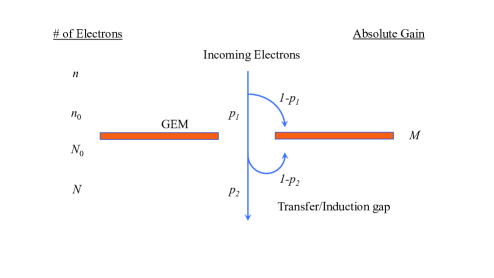
Figure 1: Notation.

The schematic view of the experimental setup is shown in Fig. 1.

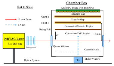
Figure 1: Schematic view of the experimental setup [26].

A pulsed UV laser beam ($\lambda$ = 266 nm) is injected into a chamber box through a quartz window at a repetition rate of 20 Hz. The chamber box contains a stack of GEM foils, a readout plane right behind the GEMs, a gating foil in front of them, and a mesh drift electrode to establish a drift field. The electrons created along a laser-induced track are selected by the gating foil, amplified by the GEMs, and then collected by the pad rows on the readout plane. The GEM foil is a copper-clad liquid crystal polymer (LCP) with holes drilled by a laser, supplied by Scienergy Co. Ltd. [48]. The thickness of the LCP is 100 $\mu$m and the hole diameter (pitch) is 70 $\mu$m (140 $\mu$m).

The transfer and induction gaps of the double GEM stack are 4 mm and 2 mm, respectively. The distance between the gating foil and the GEM stack is 9.4 mm and is referred to as the transfer region. The electric fields in the drift region and the transfer region are both set to 230 V/cm. The high voltage applied across the first (second) stage GEM is 345 V (315 V) and the electric field in the transfer (induction) gap is 900 V/cm (2700 V/cm), yielding an effective gas gain of $\sim$ 3700 with a filling gas mixture of Ar-CF₄ (3%)-isobutane (2%) at atmospheric pressure. Fig. 2 illustrates the details around the GEM stack and the gating foil.

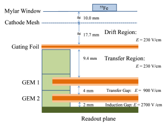
Figure 2: Schematic view of the GEM stack and the gating foil [26]. The actual setup is flipped, with the ⁵⁵Fe source placed at the bottom (see Fig. 1).

In the previous measurement of the avalanche fluctuations [25], individual signals induced on the pads were read out through multi-contact connectors arranged on the backside of the readout plane. In the present setup, on the other hand, the signal charges on the pads located at the area under study are summed on the corresponding connector and then sent to a preamplifier located nearby via a coaxial cable. Thus, the signal charge is measured on a connector-by-connector basis, instead of a pad-by-pad basis in the previous experiment. The connector reads out signals on 32 pads in adjacent two pad rows (with a pad row height of 5.26 mm), covering an area of approximately 11 mm $\times$ 19 mm on the pad plane. The output of the preamplifier is digitized by a CAMAC ADC after signal shaping. The typical number of ion pairs created along the laser-induced track is 1300 for a single connector (two pad rows). See Ref. [26] for the gating foil and the details of the experimental setup.

The variation of the average gas gain was not a serious issue in the previous measurement of avalanche fluctuations [25] and in the measurement of the transmission rate of the gating foil [26] since the duration of each run (or set of runs) was short (typically 10 minutes). On the other hand, the present measurement is based on the whole set of the laser runs. It was, therefore, important to keep the gas gain as constant as possible. Fig. 3 shows the variations in the temperature and the pressure during the laser runs.

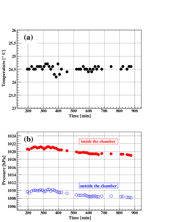
Figure 3: Variation of the temperature (a) and the pressure (b) during the laser runs.

4 Measurement Principle

In a simple case where the lateral charge spread within the gas amplification device is negligibly small compared to the readout pad (row) height such as in Micromegas, the relative variance of the gas-amplified signal charge ($R^{2}$) is given by

$$R^{2}=\frac{1+f}{\left<n\right>}$$ (3)

where $\left<n\right>$ denotes the average number of detected drift electrons while $f$ represents the relative variance of the avalanche fluctuations. In the calculation, Poisson statistics is assumed for the number of laser-induced drift electrons detected by the readout pad rows ($n$). This is a special case of the familiar formula for monochromatic photons

$$R^{2}=\frac{F+f}{\left<n\right>}\;,$$ (4)

with unity for the Fano factor ($F$) [49]. The assumption of Poisson statistics is justified also for the electrons passing through the gating foil as naively expected (see Appendix A).

In the detection of laser-induced ionizations by a GEM stack, we have to take into account the charge spread in the GEM stack as well as the laser energy fluctuations on a pulse-to-pulse basis. The value of $R^{2}$ is reduced by the signal charge sharing among adjacent pad rows due to the spread of multiplied electrons in the stack:

$$R^{2}=\frac{1+f}{\left<n\right>}\cdot g\left(\frac{\sigma}{h}\right)$$ (5)

where a reduction factor $g$ depends on the ratio of the charge spread width ($\sigma$) to the pad-row height ($h$):

$$g\left(\frac{\sigma}{h}\right)={\rm erf}\left(\frac{h}{2\sigma}\right)-\frac{2}{\sqrt{\pi}}\cdot\frac{\sigma}{h}\cdot\left[1-{\rm exp}\left(-\frac{h^{2}}{4\sigma^{2}}\right)\right]\;.$$ (6)

The value of $\sigma$ is estimated to be 341 $\mu$m from the diffusion of amplified electrons in the transfer and induction gaps, and $h$ (5.36 mm, including the gaps in-between) is to be doubled since two pad rows are covered by the single readout connector. The value of $g$ is then about 0.964 in our case where $\sigma/(2\cdot h)\sim$ 0.032.

In addition, $\left<n\right>$ fluctuates around its average $\left<\left<n\right>\right>$ because of the pulse-to-pulse variation of the laser energy, adding a constant term to Eq. (5):

$$R^{2}=\frac{1+f}{\left<\left<n\right>\right>}\cdot g\left(\frac{\sigma}{h}\right)\;+\;C^{2}$$ (7)

with

$$C^{2}=\frac{\left<\bigl{(}\left<n\right>-\left<\left<n\right>\right>\bigr{)}^{2}\right>}{\left<\left<n\right>\right>^{2}}\equiv\frac{\sigma^{2}_{\left<{\rm n}\right>}}{\left<\left<n\right>\right>^{2}}\;,$$ (8)

the relative variance of $\left<n\right>$. The derivation of Eq. (7) for the relative variance is given in Appendix B, where the evaluation of the skewness (Eq. (18) below) is also given. It is worth noting that possible hole-to-hole gas gain variation within a GEM foil does not contribute to the constant term $C^{2}$ (see Appendix C).

Since the observed average charge $\left<Q\right>$ (in ADC counts) is proportional to $\left<\left<n\right>\right>$ Eq. (7) can be rewritten as

$$R^{2}=\frac{1}{\left<Q\right>}\cdot A\cdot(1+f)\cdot g\left(\frac{\sigma}{h}\right)\;+\;C^{2}$$ (9)

with

$$A\equiv\frac{\left<Q\right>}{\left<\left<n\right>\right>}\;,$$ (10)

the average ADC counts corresponding to single drift electrons. The value of $A$ is assumed to be constant because the gas density was fairly stable throughout the experiment (see Fig. 3).

The slope ($B$) of $R^{2}$ as a function of 1/$\left<Q\right>$ is given by

$$B=A\cdot(1+f)\cdot g\left(\frac{\sigma}{h}\right)\;,$$ (11)

that contains two unknown quantities $A$ and $f$. In many cases, the constant $A$ is directly estimated using an ⁵⁵Fe source. But we did not employ this technique because of the following ambiguities.

1. The number of created ion pairs is not known precisely enough for the Penning gas mixture used.

2. The collection efficiency of the first GEM is not measured yet.

3. The leakage of the signal charge is not accurately known since only a small anode area was covered by the readout connector and the charge deposited on the surrounding area was not recorded in the laser runs.

We use instead the next normalized central moment (skewness) of the charge distribution as a function of $\left<\left<n\right>\right>$ (or $\left<Q\right>$, equivalently), assuming a Polya (gamma) distribution for the gas gain fluctuations of each drift electron [50, 51, 52], in order to obtain another relation similar to Eq. (7).

In the absence of the pulse-to-pulse laser energy fluctuations and electronic noise, the skewness is expected to be approximated by that of the compound Poisson-Polya (gamma) distribution ($S_{0}$):

$$S_{0} \equiv \frac{1}{\sqrt{\left<\left<n\right>\right>}}\cdot\frac{1+2f}{\sqrt{1+f}}$$ (12)

$$= \sqrt{\frac{A}{\left<Q\right>}}\cdot\frac{1+2f}{\sqrt{1+f}}$$

or

$$\log{S_{0}}=-\frac{1}{2}\cdot\log{\left<Q\right>}+\log{D}$$ (13)

with

$$D\equiv\sqrt{A}\cdot\frac{1+2f}{\sqrt{1+f}}\;.$$ (14)

See Appendix B for the evaluation of the skewness. The value of $D$ is the skewness at $\left<Q\right>$ = 1 and its logarithm is the y-intercept of the straight line with a slope of -1/2 representing $\log{S_{0}}$ as a function of $\log{\left<Q\right>}$.

Thus, $B$ can be determined as the slope of the straight line fitted through the relative variance ($R^{2}$) as a function of 1/$\left<Q\right>$, whereas $D$ can be obtained from the intercept (at $\left<Q\right>$ = 1) of the straight line fitted through the logarithm of the skewness ($\log{S_{0}}$) as a function of $\log{\left<Q\right>}$.

The average signal charge ($\left<Q\right>$) was controlled by changing the bias voltage ($\Delta V$) applied to the gating foil while the (average) laser pulse energy was kept constant throughout the measurement. The gating foil functions like the grid of a vacuum tube triode, or the gate of a field effect transistor (FET).

In principle, the value of $f$, as well as $A$, can readily be determined by solving the simultaneous Eqs. (11) and (14):

$$f = \frac{D-E}{2E-D}$$ (15)

$$A = E\cdot(2E-D)$$ (16)

with

$$E\equiv\sqrt{\frac{B}{g(\sigma/h)}}\;.$$ (17)

The actual analysis does not go that simply for the apparent skewnesses mainly because of the electronic noise in our case as described in the next section.

5 Results

Examples of the signal charge distribution are shown in Fig. 4 along with $\Delta V$s applied to the gating foil.

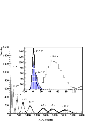
Figure 4: Examples of the signal charge distribution after pedestal subtraction obtained with the laser for different bias voltages on the gating foil [26]. A magnified view in the inset shows some of those obtained with large reverse biases.

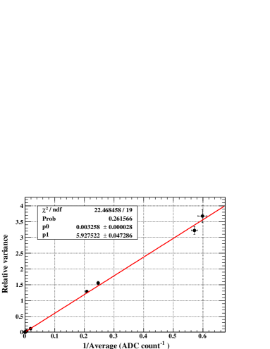
Figure 5: Relative variance of the signal charge as a function of the inverse of average ADC counts. Also shown in the figure is the straight line fitted through the data points assuming Eq. (9).

Fig. 5 shows $R^{2}$ as a function of the inverse of the average charge (1/$\left<Q\right>$).

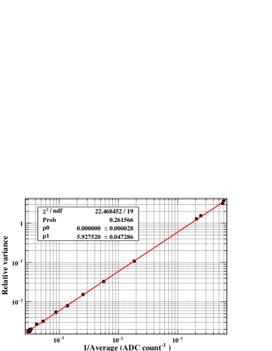
Figure 6: Log-log plot of Fig. 5 after subtraction of the constant term ($C^{2}$) from the relative variance of the signal charge.

Actually, many data points concentrate in the bottom-left corner of the figure. In order to show all the data points clearly, a log-log plot is shown in Fig. 6 after subtracting the small constant term ($C^{2}$ = 0.00326). The straight lines shown in the figures support Eq. (9). It is worth pointing out that the $y$-intercept is positive while that in the measurement with an ⁵⁵Fe source was negative (see Fig. A.1 in Ref. [26]).

A simple calculation, assuming a Polya (gamma) distribution for the avalanche fluctuations, gives a formula for the skewness ($S$):

$$S=\frac{(1+f)\cdot(1+2f)\cdot\left<\left<n\right>\right>\cdot g^{\prime}(\frac{\sigma}{h})+3\cdot(1+f)\cdot\sigma^{2}_{\left<{\rm n}\right>}\cdot g(\frac{\sigma}{h})+\left<\bigl{(}\left<n\right>-\left<\left<n\right>\right>\bigr{)}^{3}\right>+\left<\left(\Delta N\right)^{3}\right>}{\left((1+f)\cdot\left<\left<n\right>\right>\cdot g(\frac{\sigma}{h})+\sigma^{2}_{\left<{\rm n}\right>}+\left<\left(\Delta N\right)^{2}\right>\right)^{\frac{3}{2}}}$$ (18)

where $\Delta N$ represents the electronic noise with $\left<\Delta N\right>$ = 0. The functions $g$ and $g^{\prime}$ both depend on the ratio of the charge spread in the GEM stack ($\sigma$) to the pad-row height ($h$), and are given by

$$g\left(\frac{\sigma}{h}\right) \equiv \frac{1}{h}\cdot\int_{-\infty}^{+\infty}\Pi^{2}(Y)\;dY$$ (19)

$$g^{\prime}\left(\frac{\sigma}{h}\right) \equiv \frac{1}{h}\cdot\int_{-\infty}^{+\infty}\Pi^{3}(Y)\;dY$$ (20)

where $\Pi(Y)$ is defined as

$$\Pi(Y)=\int_{-h/2}^{+h/2}G(Y^{\prime};Y,\sigma)\;dY^{\prime}\;,$$ (21)

with $G(Y^{\prime};Y,\sigma)$, a Gaussian with the mean $Y$ and the standard deviation $\sigma$:

$$G(Y^{\prime};Y,\sigma)=\frac{1}{\sqrt{2\pi}\cdot\sigma}\cdot{\rm exp}\left(\frac{-(Y^{\prime}-Y)^{2}}{2\ \cdot\sigma^{2}}\right)\;.$$ (22)

See Appendix B for the derivation of Eq. (18).

In the absence of the pulse-to-pulse laser energy fluctuations ($\left<n\right>=\left<\left<n\right>\right>$), the electronic noise ($\Delta N=0$) and the charge spread ($\sigma/h=0$), the above expression for the skewness (Eq. (18)) reduces to the skewness of the compound Poisson-gamma distribution ($S_{0}$ defined by Eq. (12)) because $g(0)=g^{\prime}(0)=1$.

Using the skewness of $\left<n\right>$ distribution around $\left<\left<n\right>\right>$ ($S_{\left<{\rm n}\right>}$):

$$S_{\left<{\rm n}\right>}\equiv\frac{\left<\bigl{(}\left<n\right>-\left<\left<n\right>\right>\bigr{)}^{3}\right>}{\sigma^{3}_{\left<{\rm n}\right>}}\;,$$ (23)

with

$$\sigma^{2}_{\left<{\rm n}\right>}=C^{2}\cdot\left<\left<n\right>\right>^{2}$$ (24)

Eq. (18) can be written as

$$S=\frac{(1+f)\cdot(1+2f)\cdot g^{\prime}(\frac{\sigma}{h})\cdot\left<\left<n\right>\right>+3\cdot(1+f)\cdot g(\frac{\sigma}{h})\cdot C^{2}\cdot\left<\left<n\right>\right>^{2}+S_{\left<{\rm n}\right>}\cdot C^{3}\cdot\left<\left<n\right>\right>^{3}+\left<\left(\Delta N\right)^{3}\right>}{\left((1+f)\cdot\left<\left<n\right>\right>\cdot g(\frac{\sigma}{h})+C^{2}\cdot\left<\left<n\right>\right>^{2}+\left<\left(\Delta N\right)^{2}\right>\right)^{\frac{3}{2}}}\;.$$ (25)

The last term in the numerator is expected to be negligible since the electronic noise (pedestal) distribution is always almost Gaussian. Let us further assume that the skewness of $\left<n\right>$ ($S_{\left<{\rm n}\right>}$) is small enough to keep the third term in the numerator negligible when $\left<\left<n\right>\right>$ is not too large. Then the equation above becomes

$$S^{\prime}=\frac{(1+f)\cdot(1+2f)\cdot g^{\prime}(\frac{\sigma}{h})\cdot\left<\left<n\right>\right>+3\cdot(1+f)\cdot g(\frac{\sigma}{h})\cdot C^{2}\cdot\left<\left<n\right>\right>^{2}}{\left((1+f)\cdot g(\frac{\sigma}{h})\cdot\left<\left<n\right>\right>+C^{2}\cdot\left<\left<n\right>\right>^{2}+\left<\left(\Delta N\right)^{2}\right>\right)^{\frac{3}{2}}}\;.$$ (26)

We call hereafter the skewness given by Eq. (12) the simple model ($S_{0}$), that given by Eq. (26) the semi-realistic model ($S^{\prime}$), and that given by Eq. (25) the realistic model ($S$). These equations tell us that the skewness becomes smaller than $S_{0}$ when $\left<\left<n\right>\right>$ is small enough because of the dominance of the electronic noise term in the denominator, and that it gets larger than $S_{0}$ and approaches $S_{\left<{\rm n}\right>}$ when $\left<\left<n\right>\right>$ is large enough. For moderate values of $\left<\left<n\right>\right>$ in-between the skewness is expected to be well approximated by the simple model, depending on the size of the electronic noise and the value of $C^{2}$, since $g^{\prime}/g^{3/2}$ is close to unity with $\sigma/h\sim 0.032$. See Appendix D for the values of $C^{2}$ and $S_{\left<{\rm n}\right>}$, defined respectively by Eq. (8) and Eq. (23), expected from the specification of the laser used.

The skewness of the signal charge distribution as a function of the average ADC counts ($\left<Q\right>$) is shown in Fig. 7. Its dependence on $\left<Q\right>$ shows the expected behavior and the data points 1 to 3 seem to stay in the moderate region, where the skewness is proportional to $\left<Q\right>^{-1/2}$. The skewnesses given by the semi-realistic model are also shown in the figure. They were calculated using the pedestal widths measured for each run ($\sigma_{{\rm\Delta N}}$) and the resultant central values of $f$ and $A$ (see below). The data point (3) was excluded deliberately in the determination of $D$ defined by Eq. (14) because the value of the semi-realistic model deviates from that given by the simple model, though slightly.

The values of $f$ and $A$ were estimated to be 0.63 $\pm$ 0.16 and 3.82 $\pm$ 0.37, respectively, using Eqs. (15)-(17) with the measured values: $B=6.005\pm 0.068$, $D=3.462\pm 0.144$, and the calculated value: $g(\sigma/h)=0.9637$.

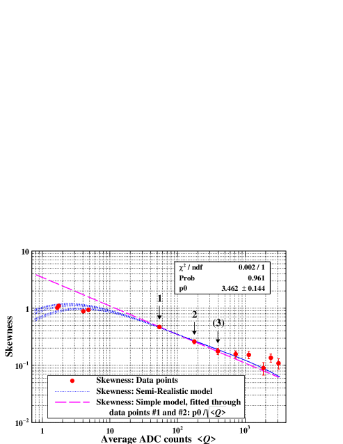
Figure 7: Skewness as a function of the average ADC counts after pedestal subtraction ($\left<Q\right>$). Filled circles for the measurements, dotted lines for the semi-realistic model (Eq. (26)), and a dashed line for the simple model (Eq. (12)). A constant term ($P0\equiv D$ defined by Eq. (14)) of the simple model was determined by fitting through two data points indicated by 1 and 2. Many curves are shown for the semi-realistic model because the contribution of electronic noise (pedestal width) varied slightly run by run. The value of $S_{\left<{\rm n}\right>}$ is expected to be $\sim$0.1 from the asymptotic skewness at large $\left<Q\right>$.

The slope ($B$) was determined by linear fitting to the data points in Fig. 6 excluding those corresponding to 1 and 2 indicated by the arrows in Fig. 7 to ensure the independence of Eqs. (11) and (14).

Since the expected error of $f$ is not small it was re-evaluated as follows. Fig. 8 shows the expected value of $D$ as a function of $f$ given by Eqs. (11) and (14):

$$D=\sqrt{\frac{B}{g(\sigma/h)}}\cdot\left(2\;-\;\frac{1}{1+f}\right)$$ (27)

along with the measured value. From the figure $f$ was determined to be $0.63^{+0.20}_{-0.16}$.

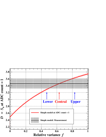
Figure 8: Value of $D$, the skewness ($S_{0}$) at ADC count = 1, as a function of $f$ given by Eq. (27) (curve) and the measured value given by the two data points 1 and 2 shown in Fig. 7 (band). The thickness (width) of the curve (band) represents the measurement error. The negative and positive errors, as well as the central value for the estimated value of $f$ are indicated by the arrows.

The relatively large statistical error of $f$ originates dominantly from the uncertainty in the value of $D$ determined by the extrapolation of the simple model down to $\left<Q\right>$ = 1 from the data points 1 and 2 in Fig. 7. The extrapolation error could have been made smaller by reducing the electronic noise in order to expand the moderate region towards the smaller $\left<Q\right>$.

For the simple model, i.e. the compound Poisson-Polya (gamma) distribution, the probability density function of the signal charge normalized by the average charge for single drift electrons ($x\equiv Q/A$) is given by

$$P(x)=e^{-\left<\left<n\right>\right>}\cdot\left(\delta(x)+\sum_{n=1}^{\infty}\frac{\left<\left<n\right>\right>^{n}}{\Gamma(n+1)}\cdot P_{n}(x)\right)$$ (28)

with

$$P_{n}(x)=\frac{(1+\theta)^{n(1+\theta)}}{\Gamma(n(1+\theta))}\cdot x^{(n-1)(1+\theta)}\cdot x^{\theta}\cdot e^{-(1+\theta)x}$$ (29)

where $\theta$ is a parameter that determines the shape of Polya (gamma) distribution ($f=1/(1+\theta)$) and $\Gamma$ denotes the gamma function. The above formula is identical to that employed in Ref. [22]. See Appendix E for the derivation of Eq. (28). Fig. 9 shows the comparison between the raw signal charge spectrum and the simple model given by Eq. (28) with the central values of $f$ and $A$.

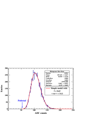
Figure 9: Observed signal charge spectrum corresponding to the data point 1 ($\Delta V$ = -12.5 V) in Fig. 7 (histogram) and that given by the simple model (Eq. (28)) normalized by the total number of events (curve).

6 Discussion

6.1 Series of our measurements

We have carried out so far three measurements of the avalanche fluctuations for the same GEM stack with the same gas mixture by means of different techniques:

1. using a laser and a pair of readout pad rows [25]

2. using an ⁵⁵Fe source and the gating foil (Appendix of Ref. [26])

3. using a laser and the gating foil (present paper),

in chronological order.

The presented value of $f$ = $0.63^{+0.20}_{-0.16}$ is consistent with our previous measurements using the differences between the laser-induced signal charges on neighboring pad rows recorded on an event-by-event (pulse-by-pulse) basis [25]. It should be noted, however, that the values of $f$ presented in Ref. [25] are underestimates since the reduction factor $g(\sigma/h)$ in Eqs. (5) and (7) due to signal charge sharing among adjacent pad rows is not taken into account. The value of $g(\sigma/h)$ for $\sigma$ = 341 $\mu$m and $h$ = 5.36 mm (for a single pad row) is about 0.928. Therefore, the values of $f=0.65\pm 0.01$ and $0.62\pm 0.01$ for the same gas mixture (Ar-CF₄ (3%)-isobutane (2%)) at gas gains of $\sim$1900 and $\sim$5800 have to be corrected to $0.78\pm 0.02$ and $0.75\pm 0.02$, respectively. Furthermore, it relied on the calibration using an ⁵⁵Fe source to determine the overall gain $A$ (average ADC counts corresponding to single drift electrons) defined by Eq. (10), that could be inaccurate (see Section 4).

If combined with a reliable calibration method the technique applied in the first measurement is attractive because it does not require any a priori assumption on the functional form of the signal charge distribution for single drift electrons (as with the second technique), and it is virtually free from the pulse-to-pulse laser energy fluctuations ($C^{2}$ in Eq. (7)) as well as from the electronic noise. In addition, a short run of $\sim$10 minutes provides sufficient statistics.

The present result is consistent also with the value of 0.84 $\pm$ 0.06 obtained in the second measurement using an ⁵⁵Fe source although it is subject to the ambiguities similar to those in the first measurement using the laser (see Appendix of Ref. [26]). It is to be noted that the second technique gives an estimate of the Fano factor as well.

The third technique presented here assumes a Polya (gamma) distribution for the avalanche fluctuations, but does not rely on the gain calibration using an ⁵⁵Fe source (monochromatic soft X-rays).

Finally, it should be pointed out that a measurement similar to the third technique is possible using an optical device such as a variable filter or a set of ND filters as described in Ref. [46], to control the average laser pulse energy. In the measurement with an ⁵⁵Fe source, on the other hand, the gating foil (or a similar device) was indispensable to control the average fraction of drift electrons contributing to the signal charge, provided that a single monochromatic X-ray source is used.

6.2 Spatial resolution of the ILD-TPC

Our measurements of the azimuthal spatial resolution of a prototype TPC with triple GEM readout [4] are consistent with the value of $N_{\rm eff}$ estimated with $f$ = 2/3 in Eq. (2) [5]. The assumed value of $f$ is a typical one for a cylindrical proportional counter operated in an argon-based mixture [53]. Our measurements of $f$ for a double GEM stack in the same gas mixture of Ar-CF₄ (3%)-isobutane (2%) at atmospheric pressure are also close to the above value (2/3) although the electric field distribution around the amplification region for GEMs is different from that in cylindrical counters. The transition of the field strength is more abrupt around the entrance of the hole in the first GEM foil. This feature of GEM (and Micromegas) is important to suppress the attachment of drift electrons to CF₄ molecules before gas multiplication.

Nevertheless, the calculated value of $f$ = 0.6 - 0.8 for cylindrical proportional counters [11] seems to be a good approximation also for a single GEM [21] as well as for Micromegas [19] operated in argon-based gas mixtures. Moreover, the value of $f$ seems to be rather insensitive to the existence of a Penning admixture (isobutane in our case). These may be due to the fact that the most part of the avalanche fluctuations is determined in the early stage of the gas multiplication in a low field region even in GEM or Micromegas (see Section 6.4). The influence of CF₄ molecules that dissociatively capture relatively hot electrons (4.5 eV - 10 eV) at the entrance to the first GEM appears to be small, if any, since the value of $N_{\rm eff}$ is comparable to those obtained with gases without CF₄ [4, 59, 60], though a small loss may have been compensated by the increase in the number of primary electrons due to the Penning effect.

In conclusion, the spatial resolution of the ILD-TPC shown in Fig. 16 of Ref. [4] with $f$ = 2/3 is expected to be reasonable, and thus the required resolution of $<$$\sim$ 100 $\mu$m is feasible over the entire sensitive volume of the ILD-TPC.

6.3 Digital TPC

If it is possible to detect each of drift electrons separately by a tiny square pad (pixel) on the readout plane after gas amplification one can get rid of the influence of avalanche fluctuations by assigning 1 to the fired pixels and 0 to the others. For TPCs with such a readout plane (digital TPCs), $f$ in Eq. (2) vanishes and the azimuthal spatial resolution of a pad row (Eq. (1)) improves. Actually, the concept of pad row does not exist anymore since there is essentially no favorable track orientation for a readout plane paved over with tiny pads. Consequently, the digital TPC is free from the resolution degradation due to the angular pad effect [8]. Furthermore, digital recording of the arrival position and time of each drift electron by tiny pads enables the cluster counting [61] and therefore improves the accuracy of the specific energy loss measurements at moderate drift distances where the merge of clusters due to transverse diffusion is not significant. The digital pixel readout gives a better energy resolution also for soft X-rays by counting the number of created ion pairs instead of the gas-amplified total charge [63, 64].

Although the digital TPC concept requires a large number of densely packed readout channels to cover the whole sensitive volume of a large TPC, promising results have been obtained using a small Micromegas with each mesh hole aligned to a readout pixel (GridPix) [65].

It should be noted that a small value of $f$, along with small electronic noise and cross-talks, is advantageous for the digital readout as well to efficiently distinguish fired pixels from those remaining quiet within the noise level.

6.4 Polya distribution

Our measurement of the relative variance relies on the assumption of the Polya (gamma) distribution for the fluctuations in the size of the avalanche initiated by a single electron (simply referred to hereafter as the avalanche fluctuations). In this subsection, some consideration is given to the validity of the assumption.

The Polya (gamma) distribution was introduced by Byrne [50, 51], and Lansiart and Morucci [52] in order to explain the observed peaked distributions for the avalanche fluctuations observed with a cylindrical proportional counter [53] and with a parallel plate chamber [66]. Their model is based on the assumption that the effective first Townsend coefficient ($\alpha^{\prime}$) is given by

$$\alpha^{\prime}(n)=\alpha\cdot\left(1+\frac{\theta}{n}\right)$$ (30)

where $\alpha$ is the first Townsend coefficient, $n$ denotes the number of electrons contained in the avalanche, and $\theta$ is the model parameter. The continuous Polya distribution (a gamma distribution) is obtained from the discrete distribution based on $\alpha^{\prime}$ using the Stirling formula, with the assumption of a large final gain and $n\gg 1$, $n\gg\theta$.

The applicability of the Polya (gamma) distribution for parallel plate geometries with a uniform electric field was criticized by Legler [67] from the viewpoint of underlying physics. He showed that the distribution based on his model with a relaxation distance ($x_{0}$) reproduced better the avalanche fluctuations observed by Schlumbohm [66] with a parallel plate chamber, in particular, for small avalanche sizes.

Alkhazov showed then that the $i$-th moment of the distributions for the Legler type models could be calculated successively for every $i$ starting from the 0-th moment (unity for the normalization of the probability density function) and the first moment (defined to be unity for the normalized average avalanche size) although they did not give an approximate analytical function for the avalanche fluctuations such as a gamma function (Polya distribution) for the Byrne–Lansiart–Morucci model [11]. He compared the moments of a variety of Legler type models (variants) and those of the Byrne–Lansiart–Morucci model for argon, with the moments given by his own realistic calculation (Eq. (56) in Ref. [11]) using the relevant cross sections consistent with the measured values of the first Townsend coefficient ($\alpha$), and found that some of the former gave a better match. He also pointed out the difference in the asymptotic behavior of the distribution for small avalanches between the Legler type models and the Byrne–Lansiart–Morucci model.

It is obvious that a photoelectron immediately after leaving the cathode with small kinetic energy needs to travel at least a finite distance ($x_{0}$) along the electric field before the first ionizing collision with a gas atom or molecule. In the simple Legler’s model, this is also the case for each of the electron pairs just after an ionizing collision throughout all stages of the avalanche growth, assuming that both of them have small kinetic energy compared to the ionization potential of the gas. It should be noted that the basic assumption (Eq. (30)) leading to the Polya (gamma) distribution implies that photoelectrons are capable of ionizing collision even immediately after the release from the cathode.

The simple Legler’s model (Model 1 in Ref. [11]) is now widely accepted as a conceptual model for the avalanche fluctuations in parallel plate geometries. The model provides a simple formula for the asymptotic value of $f$ for large avalanche size as a function of $\alpha$ and a parameter ($U_{0}$) that defines the relaxation distance ($x_{0}$). See Appendix F for the relative variance of avalanche fluctuations given by the simple Legler’s model.

It was also shown, however, that the Polya (gamma) distribution reproduced very well the avalanche fluctuations for cylindrical proportional counters up to the fourth moment (with the relative variance fixed to that given by his realistic calculation) because of the low electric field region in the very early stage of the avalanche growth, where the contribution to the final fluctuations is dominant [11]. The asymptotic behavior of the distribution for small avalanches is, on the other hand, controlled by the strong electric field near the anode wire and small avalanches are suppressed because of a large value of $a$/$\alpha$ there (see Appendix F for the definition of $a$ and the relation between $a$ and $\alpha$) [11]. As a consequence, the Polya (gamma) distribution (with an appropriate value of $\theta$) is a good match to the overall avalanche size distribution. Alkhazov illustrated the development of $f$, starting from $\sim 0$ near the cathode, towards the anode wire of a cylindrical counter given by his simplified analytical model (Fig. 5 in Ref. [11]). The analytical model, with an appropriate value of $U_{0}$, gave the value of $f$ as a function of the average size of the avalanche close to his realistic calculation (Fig. 6 in Ref. [11]).

This means that the relative variance and the skewness used in our analysis are reproduced by a Polya (gamma) distribution for cylindrical counters (operated in argon-based gas mixtures). Conversely, the Legler type models, that assume parallel-plate geometries, are inappropriate for application to the avalanche fluctuations in nonuniform electric fields. It should be pointed out, however, that the physical interpretation of the parameter ($\theta$) of the Byrne–Lansiart–Morucci model is not as clear as the relaxation distance ($x_{0}$) in the simple Legler’s model [68].

In short, the Polya (gamma) distribution is a good phenomenological or empirical model for cylindrical counter geometries to be fitted to the observed signal charge distribution for single drift electrons to obtain the value of $f$.

In general, gaseous detectors exploiting gas multiplication have a transition region between the conversion/drift region and the amplification region, where the electric field lines focus into the latter two- or three-dimensionally, except for parallel plate chambers. The simple Legler’s model is not applicable (as it is) to those gaseous detectors with a field gradient in the transition region.

An abrupt (step-function like) transition to a strong electric field in the amplification region is favorable in terms of the reduction of the avalanche fluctuations [69]. In reality, however, the transition region of the field with a finite gradient exists even for Micromegas [70], for example. The field gradient depends on the detector type (MWPC [71], MSGC [72], MGC [73], Microdot [74, 75], CGPC [76], CAT [77], Micromegas [23], GEM [9], SGC [78], PMGC [79], MCAT [80], WELL [81], MGD [82], $\mu$WD [83], MIPA [84], MHSP [85], $\mu$-PIC [86, 87], THGEM [88], $\mu$-RWELL [89] etc.), and its geometry and operating high voltages. The field gradient could therefore be quite different from that in cylindrical counters considered by Alkhazov [11]. Nevertheless, the Polya (gamma) distribution has been successfully or satisfactorily employed to fit the avalanche fluctuations obtained with various gaseous detectors including Micromegas [14, 19, 20] and a single GEM [16, 18, 21]. The avalanche fluctuation of a GEM stack is determined mostly by the first stage GEM as far as its effective gain is large enough. Hence, if the Polya (gamma) distribution is a good approximation for single GEMs so is expected for GEM stacks. See Appendix G for an evaluation of the avalanche fluctuations in a double GEM stack.

A gamma distribution ($\alpha=3/2$, $\beta=1$) was first used by Curran et al. to be fitted to the avalanche fluctuations for single photoelectrons observed with a cylindrical proportional counter [53]. It should be noted that fitting by a function (analytical or not) is necessary in many cases to estimate the relative variance by extrapolating the distribution to the region dominated by the electronic noise (pedestal region) for small signals, and to the region limited by the amplifier’s dynamic range or the ADC overflows for large signals.

Needless to say, this is not the whole story of the issue ever since the middle of the last century. See review articles such as Ref. [91] and Section 2 of Ref. [24] for its history. Our conclusion at the moment is that the Polya (gamma) distribution is expected to be a good approximation, if not the best, for the avalanche fluctuations of GEM stacks.

It should be pointed out that most of the mathematical approaches postulate the following.

1. Electron avalanche develops only by impact ionizations, without the contribution of UV photons by the photoelectric effect.

2. Space-charge effect is negligible.

3. One-dimensional treatment is justified, ignoring lateral diffusion.

4. Electric field gradient is moderate.

5. Filling gas atom/molecule has a simple structure (cross sections to the electrons) like rare gas atoms.

In reality, however, some could be inappropriate. For micro-pattern gaseous detectors (MPGDs), (3) and (4) may be the bold assumptions. The electric field experienced by the electrons approaching the amplification region depends on their paths, and they do not exactly follow the electric field lines because of diffusion. Furthermore, the local field gradient may be too large for electrons to be assumed in equilibrium with the local electric field (the value of $\alpha$ dependent only on the local electric field), or in the process to reach the equilibrium at a rate given by the local electric field and the average avalanche size there (see, for example, Eq. (51) in Ref. [11]).

An alternative way free from most of the restrictions of the mathematical approaches is the Monte-Carlo simulation of the motion of drifting electrons at the atomic level in 3-dimensional space, with all the relevant cross sections taken into account [12]. It follows the microscopic path of the individual electron in an avalanche under a given electric (and magnetic) field that may vary significantly during its free path, for any electrode configurations in virtually any gas mixtures. Potentially, it can include any physical processes neglected (or roughly approximated) so far such as the Penning effect. The microscopic Monte-Carlo simulation of avalanches is a promising approach, but is beyond the scope of the present paper.

6.5 Future prospects

The proof of principle has been demonstrated for the new technique to measure the avalanche fluctuations, and the underlying mathematics is clear. The presented measurement error is large because of the relatively large electronic noise. The noise is mostly induced by the laser and is synchronized to each laser shot (see footnote 12 of Ref. [26]). We are now preparing a dedicated smaller chamber with reduced electronic noise, along with a new laser and optical system.

The new laser may be placed away from the chamber to reduce pick-up from the laser discharge [30]. If it is difficult to suppress the noise sufficiently we can increase the drift distance of the laser-induced tracks to delay the laser signals to avoid the overlap with the laser-induced noise.

The new technique, as well as that presented in Ref. [25], will be applied to study the avalanche fluctuations for other filling gases as well, such as neon-based mixtures, in which the vale of $f$ is expected to be smaller.

7 Conclusion

In the course of performance evaluation of a gating device well suited for TPCs based on a Micro-Pattern Gaseous Detector (MPGD), we found a novel technique for the measurement of the avalanche fluctuations of gaseous detectors using UV laser-induced tracks and the gating foil. The relative variance of avalanche fluctuations ($f$) was estimated from the relative signal width and the skewness as function of (the inverse of) the average signal charge, assuming a Polya (gamma) distribution for the gas-amplified signal charge created by single drift electrons. The skewness of the signal charge distribution as a function of the average signal charge controlled by the gating foil can be used to estimate the average number of detected drift electrons, instead of the calibration using an ⁵⁵Fe source that could be inaccurate because of the ambiguity in the W-value of filling gas and/or the collection efficiency of gas-amplification device. Conversely, one can determine the average number of ion pairs created by an ⁵⁵Fe source, for example, in Penning gas mixtures for which the W-value is not precisely known if the collection efficiency is given by measurement or simulation.

The applied method gives a reasonable value of the relative variance: $f=0.63^{+0.20}_{-0.16}$ for a double GEM stack operated in a gas mixture of Ar-CF₄ (3%)-isobutane (2%) at a gas gain of $\sim$3700, which is consistent with our previous measurements. The measured values of $f$ including our previous ones are close to 2/3, which was assumed in the expected azimuthal resolution of the ILD-TPC for radial tracks better than 100 $\mu$m presented in Ref. [4]. The value of $f$ = 0.6 - 0.8 calculated for cylindrical proportional counters operated in argon-based gases [11] seems to be a good estimate also for Micromegas [19], a single GEM [21], and our double GEM stack. It is, therefore, possible to achieve the required azimuthal spatial resolution of $<$$\sim$ 100 $\mu$m for radial tracks over the entire sensitive volume of the ILD-TPC.

The measurement accuracy of the present experiment is dominated by the extrapolation error of the skewnesses of signal charge distributions, and is expected to be improved by reducing the electronic noise. We are now preparing a smaller test chamber and a new laser and optical system for the measurements with a better precision under improved conditions including a better signal to noise ratio.

Declaration of competing interest

The authors declare that they have no known competing financial interests or personal relationships that could have appeared to influence the work reported in this paper.

Appendix A Binomial selection from the uniform distribution

The electrons liberated by the laser beam drift to the front surface of the GEM stack after passing through the gating foil. Let us consider the distribution of the number of electrons reaching the surface area of the GEM stack right above a pad row. We assume a uniform (and random) spatial distribution of single electrons along the laser beam around its focal point, i.e. around the pad-row position. In addition, the diffusion of drifting electrons is ignored since it does not alter the nature of uniform distributions.

For a fixed number of the electrons reaching the surface of the gating foil above the pad row ($n_{0}$), the probability to find $n$ electrons getting through the foil is given by

$$P(n;n_{0})=\frac{n_{0}!}{n!\;(n_{0}-n)!}\cdot p^{n}\cdot(1-p)^{n_{0}-n}$$ (31)

where $p$ represents the average transmission rate of the gating foil. Since $n_{0}$ obeys Poisson statistics with a mean $\left<n_{0}\right>$, the probability mass function of $n$ is given by a compound Poisson-binomial distribution (with $\nu\equiv n_{0}-n$):

$$P(n) = e^{-\left<n_{0}\right>}\cdot\sum_{n_{0}\geq n}\frac{\left<n_{0}\right>^{n_{0}}}{n_{0}!}\cdot\frac{n_{0}!}{n!\;(n_{0}-n)!}\cdot p^{n}\cdot(1-p)^{n_{0}-n}$$ (32)

$$= e^{-\left<n_{0}\right>}\cdot\frac{p^{n}}{n!}\cdot\sum_{\nu=0}^{\infty}\frac{\left<n_{0}\right>^{\nu+n}}{\nu!}\cdot(1-p)^{\nu}$$ (33)

$$= e^{-\left<n_{0}\right>}\cdot\frac{(p\cdot\left<n_{0}\right>)^{n}}{n!}\cdot\sum_{\nu=0}^{\infty}\frac{\left(\left<n_{0}\right>\cdot(1-p)\right)^{\nu}}{\nu!}$$ (34)

$$= e^{-\left<n_{0}\right>}\cdot\frac{(p\cdot\left<n_{0}\right>)^{n}}{n!}\cdot e^{\left<n_{0}\right>\cdot(1-p)}$$ (35)

$$= e^{-p\cdot\left<n_{0}\right>}\cdot\frac{\left(p\cdot\left<n_{0}\right>\right)^{n}}{n!}\;.$$ (36)

Accordingly, the distribution of $n$ is a Poissonian with the mean $\left<n\right>=p\cdot\left<n_{0}\right>$, as naively expected.

Appendix B Evaluation of the relative variance and skewness of the signal charge distribution

Let us assume that exactly $M$ primary electrons are created by a laser pulse randomly in a region

$$-\frac{H}{2}<Y<+\frac{H}{2}\;\;{\rm with}\;\;H\gg h,\sigma$$

where $h$ is the pad-row height and $\sigma$, the standard deviation of the spread (diffusion) of multiplied electrons in the GEM stack. Then the total number of amplified electrons ($N$) detected by a pad row in $Y\in[-h/2,+h/2]$ is given by

$$N = N(Y_{1})+N(Y_{2})+\;\cdots\;+N(Y_{\rm M})$$ (37)

$$= g_{1}\cdot\Pi(Y_{1})+g_{2}\cdot\Pi(Y_{2})+\;\cdots\;+g_{\rm M}\cdot\Pi(Y_{\rm M})$$ (38)

where $N(Y_{i})$ is the number of amplified electrons in $[-h/2,+h/2]$ originated from the $i$-th primary electrons reaching the first GEM at $y=Y_{i}$, the gas gain for which is $g_{i}$, and $\Pi(Y_{i})$ is defined as

$$\Pi(Y_{i})=\int_{-h/2}^{+h/2}G(Y^{\prime};Y_{i},\sigma)\;dY^{\prime}$$ (39)

where $G(Y^{\prime};Y_{i},\sigma)$ is a Gaussian with the mean $Y_{i}$ and the standard deviation $\sigma$:

$$G(Y^{\prime};Y_{i},\sigma)=\frac{1}{\sqrt{2\pi}\cdot\sigma}\cdot{\rm exp}\left(\frac{-(Y^{\prime}-Y_{i})^{2}}{2\ \cdot\sigma^{2}}\right)\;.$$ (40)

The average value of $N$ is given by

$$\left<N\right> = M\cdot\left<g\right>\cdot\left<\Pi(Y)\right>$$ (41)

$$= M\cdot\left<g\right>\cdot\frac{h}{H}$$ (42)

$$= \rho\cdot\left<g\right>\cdot h$$ (43)

$$= \left<n\right>\cdot\left<g\right>$$ (44)

with $\rho$ being the primary ionization density ($\equiv M/H$) and $\left<n\right>\equiv\rho\cdot h$, the average number of primary electrons per pad row, using

$$\left<\Pi(Y)\right>=\frac{1}{H}\cdot\int_{-H/2}^{+H/2}\;dY\int_{-h/2}^{+h/2}G(Y^{\prime};Y,\sigma)\;dY^{\prime}=\frac{h}{H}$$ (45)

for (infinitely) large $H$ ($\gg h,\sigma$). Thus $\left<N\right>$ is not affected by the diffusion (spread) of multiplied electrons in the GEM stack.

The variance of $N$ is defined as

$$\left<\bigl{(}N-\left<N\right>\bigr{)}^{2}\right>=\left<\left(g_{1}\Pi(Y_{1})+g_{2}\Pi(Y_{2})+\;\cdots\;+g_{\rm M}\Pi(Y_{\rm M})-M\cdot\left<g\right>\cdot\frac{h}{H}\right)^{2}\right>\;.$$ (46)

For infinitely large $H$ and therefore $M$,

$$\left<g\right>=\frac{g_{1}+g_{2}+\;\cdots\;+g_{\rm M}}{M}\;.$$ (47)

Accordingly,

$$\left<\bigl{(}N-\left<N\right>\bigr{)}^{2}\right> = \left<\Biggl{(}g_{1}\left(\Pi(Y_{1})-\frac{h}{H}\right)+g_{2}\left(\Pi(Y_{2})-\frac{h}{H}\right)+\cdots+g_{\rm M}\left(\Pi(Y_{\rm M})-\frac{h}{H}\right)\Biggr{)}^{2}\right>$$ (48)

$$= \left<\left(\sum_{i=1}^{M}g_{i}\cdot\left(\Pi(Y_{i})-\frac{h}{H}\right)\right)^{2}\right>$$ (49)

$$= M\cdot\left<g^{2}\cdot\left(\Pi(Y)-\frac{h}{H}\right)^{2}\right>$$ (50)

$$= M\cdot\left<g^{2}\right>\cdot\left<\left(\Pi^{2}(Y)-\frac{2\cdot h}{H}\cdot\Pi(Y)+\frac{h^{2}}{H^{2}}\right)\right>$$ (51)

$$= M\cdot\left<g^{2}\right>\cdot\left(\left<\Pi^{2}(Y)\right>-\frac{2\cdot h}{H}\cdot\left<\Pi(Y)\right>+\frac{h^{2}}{H^{2}}\right)$$ (52)

$$= M\cdot\left<g^{2}\right>\cdot\left<\Pi^{2}(Y)\right>$$ (53)

in the limit of $H\to\infty$ with $\rho=M/H$ kept constant, and

$$\left<\Pi^{2}(Y)\right>\equiv\lim_{H\to\infty}\frac{1}{H}\int_{-H/2}^{+H/2}\Pi^{2}(Y)\;dY\;.$$ (54)

Therefore,

$$\left<\bigl{(}N-\left<N\right>\bigr{)}^{2}\right> = \lim_{H\to\infty}\frac{M}{H}\cdot\left<g^{2}\right>\cdot\int_{-H/2}^{+H/2}\Pi^{2}(Y)\;dY$$ (55)

$$= \rho\cdot h\cdot\left<g^{2}\right>\cdot\frac{1}{h}\cdot\int_{-\infty}^{+\infty}\Pi^{2}(Y)\;dY$$ (56)

$$= \left<n\right>\cdot\left<g^{2}\right>\cdot g\left(\frac{\sigma}{h}\right)$$ (57)

where $\left<n\right>\equiv\rho\cdot h$ and the function $g(\sigma/h)$ is defined as

$$g\left(\frac{\sigma}{h}\right) \equiv \frac{1}{h}\cdot\int_{-\infty}^{+\infty}\Pi^{2}(Y)\;dY$$ (58)

$$= {\rm erf}\left(\frac{h}{2\sigma}\right)-\frac{2}{\sqrt{\pi}}\cdot\frac{\sigma}{h}\cdot\left[1-{\rm exp}\left(-\frac{h^{2}}{4\sigma^{2}}\right)\right]\;.$$ (59)

See Appendix B of Ref. [6] for the evaluation of the integral in Eq. (B.22). The behavior of the function $g(\sigma/h)$ is shown in Fig. 1. For our GEM stack, $\sigma/h$ $\sim$ 0.032 and $g$ $\sim$ 0.964.

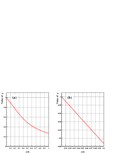
Figure 1: Value of $g$ as a function $\sigma/h$: (a) for a wide range and (b) for a practical range of $\sigma/h$.

By the same token,

$$\left<\bigl{(}N-\left<N\right>\bigr{)}^{3}\right> = \left<\Biggl{(}g_{1}\left(\Pi(Y_{1})-\frac{h}{H}\right)+g_{2}\left(\Pi(Y_{2})-\frac{h}{H}\right)+\cdots+g_{\rm M}\left(\Pi(Y_{\rm M})-\frac{h}{H}\right)\Biggr{)}^{3}\right>$$ (60)

$$= \left<\left(\sum_{i=1}^{M}g_{i}\cdot\left(\Pi(Y_{i})-\frac{h}{H}\right)\right)^{3}\right>$$ (61)

$$= M\cdot\left<g^{3}\cdot\left(\Pi(Y)-\frac{h}{H}\right)^{3}\right>$$ (62)

$$= M\cdot\left<g^{3}\right>\cdot\left<\Pi^{3}(Y)\right>$$ (63)

$$= \left<n\right>\cdot\left<g^{3}\right>g^{\prime}\left(\frac{\sigma}{h}\right)$$ (64)

where

$$g^{\prime}\left(\frac{\sigma}{h}\right)\equiv\frac{1}{h}\cdot\int_{-\infty}^{+\infty}\Pi^{3}(Y)\;dY\;.$$ (65)

The Polya distribution is often used to formulate the gas gain fluctuations for single drift electrons (see Section 6.4). Its probability density function is given by

$$P(g)=\frac{1}{\left<g\right>}\frac{(1+\theta)^{1+\theta}}{\Gamma(1+\theta)}\cdot\Bigl{(}\frac{g}{\left<g\right>}\Bigr{)}^{\theta}\cdot\exp\displaystyle\Bigl{(}-(1+\theta)\cdot\frac{g}{\left<g\right>}\Bigr{)}$$ (66)

where $\left<g\right>$ is the average gain, $\Gamma$ represents the gamma function

$$\Gamma(z)\equiv\int_{0}^{\infty}t^{z-1}\cdot e^{-t}\;dt\;\;\;{\rm for}\;\;\Re(z)>0\;,$$ (67)

and $\theta$ ( $>\;-1\,$) is a free parameter determining the shape of distribution. Let us set $x\equiv g/\left<g\right>$ and

$$P(x)=\frac{(1+\theta)^{1+\theta}}{\Gamma(1+\theta)}\cdot x^{\theta}\cdot\exp\displaystyle\Bigl{(}-(1+\theta)\cdot x\Bigr{)}$$ (68)

for $x$   >  0 .

Using integration by parts, the relevant moments are given by

$$\left<x\right> = 1$$ (69)

$$\left<x^{2}\right> = \frac{2+\theta}{1+\theta}=1+f$$ (70)

$$\left<x^{3}\right> = 1+3f+2f^{2}=(1+f)\cdot(1+2f)$$ (71)

with $f=1/(1+\theta)$, the relative variance of the distribution.

The relative variance ($R^{2}$) is therefore given by, from Eqs. (B.8) and (B.21),

$$R^{2}\equiv\frac{\left<\bigl{(}N-\left<N\right>\bigr{)}^{2}\right>}{\left<N\right>^{2}}=\frac{1+f}{\left<n\right>}\cdot g\left(\frac{\sigma}{h}\right)\;$$ (72)

and the skewness ($S$) is expressed as, from Eqs. (B.21) and (B.28),

$$S\equiv\frac{\left<\bigl{(}N-\left<N\right>\bigr{)}^{3}\right>}{\left<\bigl{(}N-\left<N\right>\bigr{)}^{2}\right>^{\frac{3}{2}}} = \frac{1}{\sqrt{\left<n\right>}}\cdot\frac{1+3f+2f^{2}}{\left(1+f\right)^{3/2}}\cdot\frac{g^{\prime}\left(\frac{\sigma}{h}\right)}{g^{3/2}\left(\frac{\sigma}{h}\right)}$$ (73)

$$= S_{0}\cdot\frac{g^{\prime}\left(\frac{\sigma}{h}\right)}{g^{3/2}\left(\frac{\sigma}{h}\right)}$$ (74)

where

$$S_{0}\equiv\frac{1}{\sqrt{\left<n\right>}}\cdot\frac{(1+f)\cdot(1+2f)}{\left(1+f\right)^{3/2}}=\frac{1}{\sqrt{\left<n\right>}}\cdot\frac{1+2f}{\sqrt{1+f}}\;.$$ (75)

It should be noted that $S_{0}$ gives the skewness in the absence of the charge spread in the GEM stack since $g(0)=g^{\prime}(0)=1$, and that $S_{0}$ reduces to $1/\sqrt{\left<n\right>}$, the skewness of Poisson distribution, in the absence of the gas gain fluctuations ($f=0$). In the present setup, the skewness of the signal charge can be well approximated by $S_{0}$, i.e. that of a compound Poisson-Polya (gamma) distribution, since the value of $g^{\prime}/g^{3/2}$ is close to unity with $\sigma/h\sim 0.032$.

In reality, $\left<n\right>$ varies around the average value ($\left<\left<n\right>\right>$) because of the pulse-to-pulse laser energy fluctuations. The values of $\left<\left(N-\left<N\right>\right)^{2}\right>$ and $\left<\left(N-\left<N\right>\right)^{3}\right>$ evaluated so far are those around the instantaneous value of $\left<g\right>\cdot\left<n\right>$ while the overall average of $N$ is given by

$$\left<\left<N\right>\right>=\left<g\right>\cdot\left<\left<n\right>\right>\;.$$ (76)

Accordingly, the relevant central moments around $\left<\left<N\right>\right>$ are given by

$$\left<\bigl{(}N-\left<\left<N\right>\right>\bigr{)}^{2}\right> = \left<\bigl{(}\left(N-\left<N\right>\right)+\left(\left<N\right>-\left<\left<N\right>\right>\right)\bigr{)}^{2}\right>$$ (77)

$$= \left<g\right>^{2}\cdot\bigintsss_{\left<n\right>}d\left<n\right>\;P\left(\left<n\right>\right)\cdot\Biggl{(}\left<n\right>\cdot(1+f)\cdot g\left(\frac{\sigma}{h}\right)+\left<\bigl{(}\left<n\right>-\left<\left<n\right>\right>\bigr{)}^{2}\right>\Biggr{)}$$ (78)

$$= \left<g\right>^{2}\cdot\Biggl{(}\left(1+f\right)\cdot\left<\left<n\right>\right>\cdot g\left(\frac{\sigma}{h}\right)+\sigma^{2}_{\left<{\rm n}\right>}\Biggr{)}\;$$ (79)

$$\left<\bigl{(}N-\left<\left<N\right>\right>\bigr{)}^{3}\right> = \left<\bigl{(}\left(N-\left<N\right>\right)+\left(\left<N\right>-\left<\left<N\right>\right>\right)\bigr{)}^{3}\right>$$

$$= \left<g\right>^{3}\cdot\int_{\left<n\right>}d\left<n\right>\;P\left(\left<n\right>\right)\cdot\left(\left(1+f\right)\cdot\left(1+2f\right)\cdot\left<n\right>\cdot g^{\prime}\left(\frac{\sigma}{h}\right)\right.$$

$$\left.+3\cdot\left(\left<n\right>-\left<\left<n\right>\right>\right)\cdot\left(1+f\right)\cdot\left<n\right>\cdot g\left(\frac{\sigma}{h}\right)+\bigl{(}\left<n\right>-\left<\left<n\right>\right>\bigr{)}^{3}\right)$$

$$= \left<g\right>^{3}\cdot\left(\left(1+f\right)\cdot\left(1+2f\right)\cdot\left<\left<n\right>\right>\cdot g^{\prime}\left(\frac{\sigma}{h}\right)\right.$$

$$\left.+3\cdot\left(1+f\right)\cdot\sigma^{2}_{\left<{\rm n}\right>}\cdot g\left(\frac{\sigma}{h}\right)+\bigl{(}\left<n\right>-\left<\left<n\right>\right>\bigr{)}^{3}\right)$$ (82)

where $P(\left<n\right>)$ is the probability density function for $\left<n\right>$ and $\sigma^{2}_{\left<{\rm n}\right>}\equiv\left<\bigl{(}\left<n\right>-\left<\left<n\right>\right>\bigr{)}^{2}\right>$.

In addition, the signal charge is accompanied by the electronic noise ($\Delta N$) in real measurements. Taking the average charge corresponding to a single drift electron after gas multiplication and electronic amplification as the unit of $\Delta N$, and assuming $\left<\Delta N\right>$ = 0,

$$\left<\bigl{(}N+\Delta N-\left<\left<N\right>\right>\bigr{)}^{2}\right> = \left<\bigl{(}N-\left<\left<N\right>\right>\bigr{)}^{2}\right>+\left<\bigl{(}\Delta N\bigr{)}^{2}\right>$$ (83)

$$\left<\bigl{(}N+\Delta N-\left<\left<N\right>\right>\bigr{)}^{3}\right> = \left<\bigl{(}N-\left<\left<N\right>\right>\bigr{)}^{3}\right>+\left<\bigl{(}\Delta N\bigr{)}^{3}\right>\;.$$ (84)

For the variance, the contribution of the electronic noise to be subtracted from the raw variance is estimated from the pedestal width. The net relative variance of the signal ($\equiv$ $R^{2}$) is therefore given, from Eqs. (B.40) and (B.43), by

$$R^{2} = \frac{\left<\bigl{(}N-\left<\left<N\right>\right>\bigr{)}^{2}\right>}{\left<\left<N\right>\right>^{2}}$$ (85)

$$= \frac{1+f}{\left<\left<n\right>\right>}\cdot g\left(\frac{\sigma}{h}\right)\;+\;\frac{\sigma^{2}_{\left<{\rm n}\right>}}{\left<\left<n\right>\right>^{2}}\;.$$ (86)

On the other hand, the skewness ($S$) is expressed as, from Eqs. (B.43), (B.46), (B.47) and (B.48),

$$S=\frac{(1+f)\cdot(1+2f)\cdot\left<\left<n\right>\right>\cdot g^{\prime}(\frac{\sigma}{h})+3\cdot(1+f)\cdot\sigma^{2}_{\left<{\rm n}\right>}\cdot g(\frac{\sigma}{h})+\left<\bigl{(}\left<n\right>-\left<\left<n\right>\right>\bigr{)}^{3}\right>+\left<\left(\Delta N\right)^{3}\right>}{\left((1+f)\cdot\left<\left<n\right>\right>\cdot g(\frac{\sigma}{h})+\sigma^{2}_{\left<{\rm n}\right>}+\left<\left(\Delta N\right)^{2}\right>\right)^{\frac{3}{2}}}\;.$$ (87)

In the absence of the laser pulse-energy fluctuations ($\left<n\right>=\left<\left<n\right>\right>$), the electronic noise ($\Delta N=0$) and the charge spread in the GEM stack ($\sigma/h=0$), the above expression for the skewness reduces to $S_{0}$ because $g(0)=g^{\prime}(0)=1$.

Appendix C Influence of the hole-to-hole gain variation on the signal width

We evaluate here the influence of the hole-to-hole variation of the average gas gain within a simplified virtual GEM foil, on the width of the total number of electrons detected by a readout pad row (or a pair of pad rows, in our case) in the laser experiment.

Let us assume that there are infinite number of infinitesimal GEM holes along the laser induced tracks and a set of firing holes is selected randomly on a track-by-track basis. The average gain of each GEM hole ($\left<g_{i}\right>$) is distributed around the overall average gain ($\left<\left<g\right>\right>$) with a standard deviation of $\sigma_{\left<{\rm g}\right>}$, whereas the relative variances of the gain fluctuations ($f\equiv\sigma_{{\rm g}_{i}}^{2}/\left<g_{i}\right>^{2}$) are assumed to be identical. The charge sharing between adjacent pad rows is ignored throughout the following calculation just to simplify the description. We assume a constant laser pulse energy as well and, therefore, Poisson statistics for the number of drift electrons ($n$) detected by the pad row.

The number of amplified electrons detected by the pad row is then given by

$$N = \sum_{i=1}^{n}g_{i}$$ (88)

$$= \sum_{i=1}^{n}\bigl{(}\left<g_{i}\right>+\delta g_{i}\bigr{)}$$ (89)

$$\left<N\right> = \left<n\right>\cdot\left<\left<g\right>\right>$$ (90)

where $g_{i}$ is the gas gain of the GEM hole hit by the drift electron $i\/$. The value of $\left<n\right>$ is given by $\rho\cdot h$ with $\rho$ being the average laser ionization density and $h$, the length along the laser induced tracks covered by the pad row.

The variance of the total number of signal electrons is given by

$$\left<\bigl{(}N-\left<N\right>\bigr{)}^{2}\right> = \left<\left(\sum_{i=1}^{n}\bigl{(}\left<g_{i}\right>+\delta g_{i}\bigr{)}-\left<n\right>\cdot\left<\left<g\right>\right>\right)^{2}\right>$$ (91)

$$= \left<\left(\sum_{i=1}^{n}\bigl{(}\left<g_{i}\right>+\delta g_{i}\bigr{)}-n\cdot\left<\left<g\right>\right>+n\cdot\left<\left<g\right>\right>-\left<n\right>\cdot\left<\left<g\right>\right>\right)^{2}\right>$$ (92)

$$= \left<\left(\sum_{i=1}^{n}\bigl{(}\left<g_{i}\right>-\left<\left<g\right>\right>+\delta g_{i}\bigr{)}+\bigl{(}n-\left<n\right>\bigr{)}\cdot\left<\left<g\right>\right>\right)^{2}\right>$$ (93)

$$= \left<n\cdot\bigl{(}\left<g_{i}\right>-\left<\left<g\right>\right>+\delta g_{i}\bigr{)}^{2}\right>+\left<\bigl{(}n-\left<n\right>\bigr{)}^{2}\right>\cdot\left<\left<g\right>\right>^{2}$$ (94)

$$= \left<n\right>\cdot\biggl{(}\left<\bigl{(}\left<g_{i}\right>-\left<\left<g\right>\right>\bigr{)}^{2}\right>+\left<\left<\left(\delta g_{i}\right)^{2}\right>\right>\biggr{)}+\left<n\right>\cdot\left<\left<g\right>\right>^{2}$$ (95)

$$= \left<n\right>\cdot\biggl{(}\sigma_{\left<{\rm g}\right>}^{2}+f\cdot\left(\left<\left<g\right>\right>^{2}+\sigma_{\left<{\rm g}\right>}^{2}\right)\biggr{)}+\left<n\right>\cdot\left<\left<g\right>\right>^{2}$$ (96)

$$= \left<n\right>\cdot\biggl{(}\left<\left<g\right>\right>^{2}+\sigma_{\left<{\rm g}\right>}^{2}+f\cdot\left(\left<\left<g\right>\right>^{2}+\sigma_{\left<{\rm g}\right>}^{2}\right)\biggr{)}$$ (97)

$$= \left<n\right>\cdot\left<\left<g\right>\right>^{2}\cdot\left(1+f\right)\cdot\big{(}1+\frac{\sigma_{\left<{\rm g}\right>}^{2}}{\left<\left<g\right>\right>^{2}}\bigr{)}$$ (98)

where

$$\left<\left(\delta g_{i}\right)^{2}\right> = f\cdot\left<g_{i}\right>^{2}$$ (99)

$$\left<\left<\left(\delta g_{i}\right)^{2}\right>\right> = f\cdot\left<\left<g_{i}\right>^{2}\right>$$ (100)

$$= f\cdot\left(\left<\left<g\right>\right>^{2}+\sigma_{\left<{\rm g}\right>}^{2}\right)\;.$$ (101)

The relative variance of the total number of detected electrons is, therefore, given by

$$\frac{\left<\bigl{(}N-\left<N\right>\bigr{)}^{2}\right>}{\left<N\right>^{2}}=\frac{1}{\left<n\right>}\cdot\left(1+f\right)\cdot\big{(}1+\frac{\sigma_{\left<{\rm g}\right>}^{2}}{\left<\left<g\right>\right>^{2}}\bigr{)}\;.$$ (102)

The simplified model shows that the relative variance of the signal charge is a linear function of $1/\left<n\right>$ with a slope ($s$) of

$$s=\left(1+f\right)\cdot\big{(}1+\frac{\sigma_{\left<{\rm g}\right>}^{2}}{\left<\left<g\right>\right>^{2}}\bigr{)}\;.$$ (103)

As a consequence, the hole-to-hole gain variation makes the apparent value of $f$ slightly large. For example, if $\sigma_{\left<{\rm g}\right>}/\left<\left<g\right>\right>$ = 10% and $f$ = 0.6 (0.7) the ${\it observed}$ value of $f$ would be 0.616 (0.717). It should also be noted that the hole-to-hole gain variation assumed in this model does not add an offset ($y$-intercept) to the linear relation between the relative variance of the signal charge and the inverse of the average charge (proportional to $\left<n\right>$).

In the case of monochromatic X-rays (from an ⁵⁵Fe source, for example), a similar calculation gives

$$\frac{\left<\bigl{(}N-\left<N\right>\bigr{)}^{2}\right>}{\left<N\right>^{2}}=\frac{1}{\left<n\right>}\cdot\left(F+\frac{\sigma_{\left<{\rm g}\right>}^{2}}{\left<\left<g\right>\right>^{2}}+f\cdot\big{(}1+\frac{\sigma_{\left<{\rm g}\right>}^{2}}{\left<\left<g\right>\right>^{2}}\bigr{)}\right)\;$$ (104)

with $F$, the Fano factor. The above equation reduces to the familiar formula

$$\frac{\left<\bigl{(}N-\left<N\right>\bigr{)}^{2}\right>}{\left<N\right>^{2}}=\frac{1}{\left<n\right>}\cdot\left(F+f\right)\;$$ (105)

without the gain variation ($\sigma_{\left<{\rm g}\right>}$ = 0) while it reduces to Eq. (C.15) when the distribution of $n$ is Poissonian ($F=1$).

Appendix D Relative variance and skewness of the laser-induced ionizations

In this appendix, we estimate the expected values of the relative variance and the skewness of the distribution of the number of laser-induced ionizations in a small interval along the laser beam covered by the readout pad row(s) ($\Delta z$). In the following, a simple model is assumed for the ionization process:

1. The laser-induced ionization is caused by a double-photon interaction with an unidentified impurity molecule in the filling gas via an intermediate excited state with a lifetime much longer than the duration of a laser pulse, but shorter than the pulse interval [43].

2. The impurity molecules are assumed to be at rest (stationary targets), like in a still picture taken with a short exposure time, because their thermal diffusion (random walk distance) during the pulsed laser irradiation is small. This means that the excitation and possible subsequent ionization occur in the same spot.

3. The laser flux is moderate and its duration is short enough so that the vast majority of the impurity molecules stay at the ground state during the irradiation.

We assume a simple model also for the pulsed laser beam, that allows separation (and disregard) of relevant variables. Let us set $\phi(\boldsymbol{x},z,t;t^{*})$ to be the local photon flux (photons/unit area/sec) where $\boldsymbol{x}\equiv(x,y)$, with the z-coordinate axis along the laser beam, $t$ denotes time in the duration of a pulse measured from its start time ($t^{*}$). The discrete variable $t^{*}$ is the time stamp for each pulse and the symbol $\left<\cdots\right>$ for a function of $t^{*}$ in the following denotes the average over pulses.

First, we neglect its $z$-dependence in a small interval $\Delta z$:

$$\phi(\boldsymbol{x},z,t;t^{*})=\phi(\boldsymbol{x},t;t^{*})$$ (106)

at any given time ($t$) during a pulse. Next, we suppose that the time dependence of photon flux is independent of $\boldsymbol{x}$:

$$\phi(\boldsymbol{x},t;t^{*})=f(\boldsymbol{x};t^{*})\cdot a(t)\;$$ (107)

with

$$\int_{0}^{T}a(t)\;dt=1\;$$ (108)

where $T$ denotes the duration of pulses. It should be noted that the function $a(t)$ is bell-shaped with a peak near the middle of the pulse duration, and with a small positive skewness in our case. Its duration is about 3-4 nsec at FWHM, which corresponds to the width in space (beam length) of $\sim$1 m (FWHM) along z-axis. Therefore, the z-dependence of the flux at any given $t$ is small and Eq. (D.1) is expected to be a reasonable approximation since the beam length is large compared to $\Delta z$ ($\sim$10 mm, in our case).

Finally, the shape of photon density in the $x$-$y$ plane is assumed to be identical for all the pulses:

$$f(\boldsymbol{x};t^{*})=f_{0}(\boldsymbol{x})\cdot\left(1+\epsilon(t^{*})\right)$$ (109)

where $f_{0}(\boldsymbol{x})$ is the local fluence at $\boldsymbol{x}$ averaged over pulses with $\left<\epsilon(t^{*})\right>$ = 0, and

$$\epsilon(t^{*}) = \frac{f(\boldsymbol{x};t^{*})-f_{0}(\boldsymbol{x})}{f_{0}(\boldsymbol{x})}$$ (110)

$$\equiv \frac{\delta f(\boldsymbol{x};t^{*})}{f_{0}(\boldsymbol{x})}\;.$$ (111)

In short, we consider repeated irradiations on a thin layer of impurity molecules by a series of laser pulses with an identical shape of the beam profile, and with each being characterized only by the total number of photons, except for the statistical fluctuations in the number of photons distributed to each section in the profile.

Now, let us consider the probability that an impurity molecule staying at $\boldsymbol{x}$ is ionized in a time interval [$t_{2},\;t_{2}+\Delta t$] measured from the beginning of a pulse ($t^{*}$). We define $\sigma_{\rm ex}$ to be the cross section of the impurity molecule for the transition from the ground state to the excited state, and $\sigma_{\rm i}$ to be that for the transition from the excited state to the ionized (continuum) state. Since the molecule needs to have been excited before $t_{2}$ the probability is given by

$$P(t_{2})\;\cdot\Delta t = \Delta t\cdot f(\boldsymbol{x};t^{*})\cdot a(t_{2})\cdot\sigma_{\rm i}\cdot\int_{0}^{t_{2}}f(\boldsymbol{x};t^{*})\cdot a(t_{1})\cdot\sigma_{\rm ex}\;dt_{1}$$ (112)

$$= \Delta t\cdot f^{2}(\boldsymbol{x};t^{*})\cdot\sigma_{\rm i}\cdot\sigma_{\rm ex}\cdot a(t_{2})\cdot\int_{0}^{t_{2}}a(t_{1})\;dt_{1}\;.$$ (113)

The probability for the molecule to be ionized during the pulse is then given by

$$\int_{0}^{T}P(t_{2})\;dt_{2} = \sigma_{\rm i}\cdot\sigma_{\rm ex}\cdot f^{2}(\boldsymbol{x};t^{*})\cdot\int_{0}^{T}a(t_{2})\;dt_{2}\;\int_{0}^{t_{2}}a(t_{1})\;dt_{1}$$ (114)

$$= \sigma_{\rm i}\cdot\sigma_{\rm ex}\cdot f^{2}(\boldsymbol{x};t^{*})\cdot\int_{0}^{T}\frac{d}{dt_{2}}\Biggl{(}\int_{0}^{t_{2}}a(t^{\prime})\;dt^{\prime}\Biggr{)}\;dt_{2}\cdot\int_{0}^{t_{2}}a(t_{1})\;dt_{1}$$ (115)

$$= \sigma_{\rm i}\cdot\sigma_{\rm ex}\cdot f^{2}(\boldsymbol{x};t^{*})\cdot\int_{0}^{T}A(t_{2})\cdot\frac{dA(t_{2})}{dt_{2}}\;dt_{2}$$ (116)

with

$$A(t_{2})\equiv\int_{0}^{t_{2}}a(t^{\prime})\;dt^{\prime}\;.$$ (117)

The integral can be evaluated by partial integration:

$$\int_{0}^{T}A(t_{2})\cdot\frac{dA(t_{2})}{dt_{2}}\;dt_{2} = \Bigl{[}A^{2}(t_{2})\Bigr{]}_{0}^{T}-\int_{0}^{T}A(t_{2})\cdot\frac{dA(t_{2})}{dt_{2}}\;dt_{2}$$ (118)

$$= \frac{1}{2}\cdot\Bigl{[}A^{2}(t_{2})\Bigr{]}_{0}^{T}$$ (119)

$$= \frac{1}{2}\cdot\Biggl{(}\int_{0}^{T}a(t^{\prime})\;dt^{\prime}\Biggr{)}^{2}$$ (120)

$$= \frac{1}{2}\;.$$ (121)

Multiplying the number of target molecules, the average number of ionizations around $\boldsymbol{x}$ is given by

$$\overline{n}(\boldsymbol{x};t^{*})\;d\boldsymbol{x}=c\cdot f^{2}(\boldsymbol{x};t^{*})\;d\boldsymbol{x}\;$$ (122)

where

$$c=\frac{1}{2}\cdot\sigma_{\rm i}\cdot\sigma_{\rm ex}\cdot\rho\cdot\Delta z$$ (123)

with $\rho$, the density of the impurity molecules at the ground state.

The average total number of created electrons for the pulse with a time stamp $t^{*}$ is then given by

$$\overline{n}(t^{*}) = \int\overline{n}(\boldsymbol{x};t^{*})\;d\boldsymbol{x}$$ (124)

$$= c\cdot\int f^{2}(\boldsymbol{x};t^{*})\;d\boldsymbol{x}$$ (125)

$$= c\cdot\bigl{(}1+\epsilon(t^{*})\bigr{)}^{2}\cdot\int f_{0}^{2}(\boldsymbol{x})\;d\boldsymbol{x}$$ (126)

and its average over $t^{*}$ (pulses) is

$$\left<\left<n\right>\right> \equiv \left<\overline{n}(t^{*})\right>$$ (127)

$$= c\cdot\left<\bigl{(}1+\epsilon(t^{*})\bigr{)}^{2}\right>\cdot\int f_{0}^{2}(\boldsymbol{x})\;d\boldsymbol{x}$$ (128)

$$= c\cdot\left(1+\sigma^{2}\right)\cdot\int f_{0}^{2}(\boldsymbol{x})\;d\boldsymbol{x}\;$$ (129)

with

$$\sigma^{2}\equiv\left<\epsilon^{2}(t^{*})\right>\;.$$ (130)

Actually, $\sigma$ is the standard deviation of the fractional variation of the total number of photons in a pulse:

$$\sigma=\frac{\sqrt{\left<\bigl{(}\delta f(\boldsymbol{x};t^{*})\bigr{)}^{2}\right>}}{f_{0}(\boldsymbol{x})}\equiv\frac{\sigma_{\rm f}(\boldsymbol{x})}{f_{0}(\boldsymbol{x})}=\frac{\sigma_{\rm F}}{\left<F\right>}\;$$ (131)

where

$$\left<F\right>\equiv\int f_{0}(\boldsymbol{x})\;d\boldsymbol{x}$$ (132)

and

$$\sigma_{\rm F}^{2} = \left<\bigl{(}\delta F(t^{*})\bigr{)}^{2}\right>$$ (133)

$$\equiv \left<\bigl{(}F(t^{*})-\left<F\right>\bigr{)}^{2}\right>$$ (134)

$$= \left<\epsilon^{2}(t^{*})\right>\cdot\left<F\right>^{2}$$ (135)

$$= \sigma^{2}\cdot\left<F\right>^{2}$$ (136)

with

$$F(t^{*}) \equiv \int f(\boldsymbol{x};t^{*})\;d\boldsymbol{x}$$ (137)

$$= \int\bigl{(}1+\epsilon(t^{*})\bigr{)}\cdot f_{0}(\boldsymbol{x})\;d\boldsymbol{x}$$ (138)

$$= \bigl{(}1+\epsilon(t^{*})\bigr{)}\cdot\left<F\right>\;.$$ (139)

Here $\left<F\right>$ represents the average total number of photons in a pulse, which is proportional to the average laser pulse energy. It should be noted that the average number of ionizations is proportional to the square of the average pulse energy since $\left<\left<n\right>\right>$ is quadrupled while $\left<F\right>$ is doubled when $f_{0}(\boldsymbol{x})$ is uniformly doubled over $\boldsymbol{x}$, for example, according to Eqs. (D.24) and (D.27).

The distribution of $\epsilon(t^{*})$ is more or less Gaussian for our new laser system of a similar type (Litron Nano S 120-20-FHG) although we did not have a chance to measure it for New Wave Research Polaris II used in the present experiment. Let us therefore suppose further that the random variable

$$r\equiv\epsilon(t^{*})=\frac{\delta F(t^{*})}{\left<F\right>}$$ (140)

is Gaussian distributed with a standard deviation of $\sigma$. The assumption simplifies the following calculations since

$$\left<\epsilon^{6}(t^{*})\right>=15\cdot\sigma^{6},\;\;\left<\epsilon^{4}(t^{*})\right>=3\cdot\sigma^{4},\;\;\left<\epsilon^{2}(t^{*})\right>\equiv\sigma^{2}$$ (141)

while

$$\left<\epsilon^{5}(t^{*})\right>=\left<\epsilon^{3}(t^{*})\right>=\left<\epsilon(t^{*})\right>=0$$ (142)

with $\sigma=\sigma_{\rm F}/\left<F\right>$.

The variance of the average number of created electrons in this case is given by

$$\left<\bigl{(}\overline{n}(t^{*})-\left<\left<n\right>\right>\bigr{)}^{2}\right> = c^{2}\cdot\left<\left(\left(1+\epsilon(t^{*})\right)^{2}-\left(1+\sigma^{2}\right)\right)^{2}\right>\cdot\left(\int f_{0}^{2}(\boldsymbol{x})\;d\boldsymbol{x}\right)^{2}$$ (143)

$$= 4\cdot c^{2}\cdot\sigma^{2}\cdot\left(1+\frac{1}{2}\cdot\sigma^{2}\right)\cdot\left(\int f_{0}^{2}(\boldsymbol{x})\;d\boldsymbol{x}\right)^{2}\;$$ (144)

and the relative variance is, from Eqs. (D.24) and (D.39),

$$\frac{\left<\bigl{(}\overline{n}(t^{*})-\left<\left<n\right>\right>\bigr{)}^{2}\right>}{\left<\left<n\right>\right>^{2}} = 4\cdot\sigma^{2}\cdot\frac{1+\frac{1}{2}\cdot\sigma^{2}}{\left(1+\sigma^{2}\right)^{2}}$$ (145)

$$= 4\cdot\frac{\sigma_{\rm F}^{2}}{\left<F\right>^{2}}\cdot\frac{1+\frac{1}{2}\cdot\frac{\sigma_{\rm F}^{2}}{\left<F\right>^{2}}}{\left(1+\frac{\sigma_{\rm F}^{2}}{\left<F\right>^{2}}\right)^{2}}\;.$$ (146)

Similarly,

$$\left<\bigl{(}\overline{n}(t^{*})-\left<\left<n\right>\right>\bigr{)}^{3}\right> = c^{3}\cdot\left<\left(\bigl{(}1+\epsilon(t^{*})\bigr{)}^{2}-\left(1+\sigma^{2}\right)\right)^{3}\right>\cdot\left(\int f_{0}^{2}(\boldsymbol{x})\;d\boldsymbol{x}\right)^{3}$$ (147)

$$= 24\cdot c^{3}\cdot\sigma^{4}\cdot\left(1+\frac{1}{3}\cdot\sigma^{2}\right)\cdot\left(\int f_{0}^{2}(\boldsymbol{x})\;d\boldsymbol{x}\right)^{3}\;$$ (148)

and the skewness is given by, from Eqs. (D.39) and (D.43),

$$\frac{\left<\bigl{(}\overline{n}(t^{*})-\left<\left<n\right>\right>\bigr{)}^{3}\right>}{\left<\bigl{(}\overline{n}(t^{*})-\left<\left<n\right>\right>\bigr{)}^{2}\right>^{\frac{3}{2}}} = 3\cdot\sigma\cdot\frac{1+\frac{1}{3}\cdot\sigma^{2}}{\left(1+\frac{1}{2}\cdot\sigma^{2}\right)^{\frac{3}{2}}}$$ (149)

$$= 3\cdot\frac{\sigma_{\rm F}}{\left<F\right>}\cdot\frac{1+\frac{1}{3}\cdot\frac{\sigma_{\rm F}^{2}}{\left<F\right>^{2}}}{\left(1+\frac{1}{2}\cdot\frac{\sigma_{\rm F}^{2}}{\left<F\right>^{2}}\right)^{\frac{3}{2}}}\;.$$ (150)

The specification for the pulse energy stability of the laser used (New Wave Research Polaris II) is $\pm$ 6% for 98% of pulses. If the distribution of $r=\delta F(t^{*})/\left<F\right>$ is Gaussian, the 98%-containment corresponds to $\pm$ 2.3 standard deviations and the limit of $\pm$ 6% gives 2.6% for $\sigma_{\rm F}/\left<F\right>$. The relative variance and the skewness of the $\overline{n}$ distribution are, therefore, expected to be about 0.0027 and 0.078, respectively, from Eqs. (D.41) and (D.45). Our model, though possibly oversimplified, gives the values close to the observed ones: 0.0033 for the relative variance $C^{2}$ (see Eqs. (8) and (9), and Fig. 5) and $\sim$0.1 for the skewness $S_{\left<n\right>}$, that is expected to be the asymptotic value of the skewness of the signal charge distribution ($S$) for large $\left<Q\right>$ (see Fig. 7 and text).

The same results can be obtained easily by assuming a simple structure of the pulsed laser beam, i.e. a rectangular distribution both in space and time. This simplification is justified because the laser beam profile in the $x$-$y$ plane at any given time during a pulse can be assumed to be a set of independent square column-like distributions like a lego plot as far as the impurity molecules are stationary targets, and the number of local ionizations $\overline{n}(\boldsymbol{x},t^{*})$ does not depend on the shape of time structure ($a(t^{\prime})$, see Eq. (D.17)) including a uniform (rectangular) distribution.

Appendix E Signal charge distribution in the ideal case

In this appendix, we present the signal charge distribution in the ideal case, i.e. in the absence of the charge spread in the GEM stack, the laser pulse-energy fluctuations and the electronic noise. As in Appendix B, we assume that the probability density function of $x\equiv g/\left<g\right>$, the gas gain ($g$) normalized by its average ($\left<g\right>$), for single drift electrons is given by

$$P_{1}(x)=A\cdot x^{\theta}\cdot\exp\displaystyle\Bigl{(}-(1+\theta)\cdot x\Bigr{)}$$ (151)

with

$$A\equiv\frac{(1+\theta)^{1+\theta}}{\Gamma(1+\theta)}\;$$ (152)

for the continuous random variable $x\;>\;0$, where $\Gamma$ represents the gamma function defined in Appendix B (Eq. (B.31)), and $\theta$ ($>-1$) is a parameter determining the shape of distribution ($f=1/(1+\theta)$).

The charge distribution for two drift electrons, scaled by $\left<g\right>$, is then given by

$$P_{2}(x) = A^{2}\cdot\int_{0}^{x}dx_{1}\int_{0}^{x}dx_{2}\;(x_{1}\cdot x_{2})^{\theta}\cdot e^{-(1+\theta)\cdot(x_{1}+x_{2})}\cdot\delta(x-x_{1}-x_{2})$$ (153)

$$= A^{2}\cdot e^{-(1+\theta)x}\cdot\int_{0}^{x}dx_{1}\bigl{(}x_{1}\cdot(x-x_{1})\bigr{)}^{\theta}$$ (154)

$$= A^{2}\cdot e^{-(1+\theta)x}\cdot\int_{0}^{1}(x\cdot t)^{\theta}\cdot(x-x\cdot t)^{\theta}\cdot x\cdot dt\;\;\;{\rm with}\;\;t\equiv\frac{x_{1}}{x}$$ (155)

$$= A^{2}\cdot e^{-(1+\theta)x}\cdot x^{(1+2\theta)}\cdot\int_{0}^{1}t^{\theta}(1-t)^{\theta}dt$$ (156)

$$= A^{2}\cdot B(1+\theta,1+\theta)\cdot x^{1+\theta}\cdot x^{\theta}\cdot e^{-(1+\theta)x}$$ (157)

where $B$ represents the beta function

$$B(\alpha,\beta)\equiv\int_{0}^{1}t^{\alpha-1}\cdot(1-t)^{\beta-1}\;dt=\frac{\Gamma(\alpha)\cdot\Gamma(\beta)}{\Gamma(\alpha+\beta)}\;.$$ (158)

The normalization constant is expressed as

$$A^{2}\cdot B(1+\theta,1+\theta) = \left(\frac{(1+\theta)^{1+\theta}}{\Gamma(1+\theta)}\right)^{2}\cdot\frac{\left(\Gamma(1+\theta)\right)^{2}}{\Gamma(2(1+\theta))}$$ (159)

$$= \frac{(1+\theta)^{2(1+\theta)}}{\Gamma(2(1+\theta))}\;.$$ (160)

Accordingly

$$P_{2}(x)=\frac{(1+\theta)^{2(1+\theta)}}{\Gamma(2(1+\theta))}\cdot x^{1+\theta}\cdot x^{\theta}\cdot e^{-(1+\theta)x}\;.$$ (161)

Similarly, the charge distribution for three drift electrons scaled by $\left<g\right>$ is given by, with

$$x^{\prime}\equiv x_{1}+x_{2},\;\;C\equiv A^{2}\cdot B(1+\theta,1+\theta)=\frac{(1+\theta)^{2(1+\theta)}}{\Gamma(2(1+\theta))},\;\;{\rm and}\;t\equiv\frac{x_{3}}{x}\;,$$ (162)

$$P_{3}(x) = \int_{0}^{x}dx_{3}\int_{0}^{x}dx^{\prime}\;P_{1}(x_{3})\cdot P_{2}(x^{\prime})\cdot\delta(x-x^{\prime}-x_{3})$$ (163)

$$= A\cdot\ C\cdot e^{-(1+\theta)x}\cdot\int_{0}^{x}dx_{3}\;\int_{0}^{x}dx^{\prime}\;x_{3}^{\theta}\cdot(x^{\prime})^{1+\theta}\cdot(x^{\prime})^{\theta}\cdot\delta(x-x^{\prime}-x_{3})$$ (164)

$$= A\cdot\ C\cdot e^{-(1+\theta)x}\cdot\int_{0}^{x}dx_{3}\;x_{3}^{\theta}\cdot\left(x-x_{3}\right)^{1+2\theta}$$ (165)

$$= A\cdot\ C\cdot e^{-(1+\theta)x}\cdot\int_{0}^{1}x\;dt\;(x\cdot t)^{\theta}\cdot(x-x\cdot t)^{1+2\theta}$$ (166)

$$= A\cdot\ C\cdot e^{-(1+\theta)x}\cdot x^{\theta}\cdot x^{2(1+\theta)}\cdot\int_{0}^{1}t^{\theta}\cdot(1-t)^{1+2\theta}\;dt$$ (167)

$$= A\cdot\ C\cdot B(1+\theta,2(1+\theta))\cdot x^{2(1+\theta)}\cdot x^{\theta}\cdot e^{-(1+\theta)x}\;$$ (168)

where

$$B(1+\theta,2(1+\theta))=\frac{\Gamma(1+\theta)\cdot\Gamma(2(1+\theta))}{\Gamma(3(1+\theta))}\;.$$ (169)

The normalization constant is then

$$A\cdot C\cdot B(1+\theta,2(1+\theta)) = A^{3}\cdot B(1+\theta,1+\theta)\cdot B(1+\theta,2(1+\theta))$$ (170)

$$= \frac{(1+\theta)^{1+\theta}}{\Gamma(1+\theta)}\cdot\frac{(1+\theta)^{2(1+\theta)}}{\Gamma(2(1+\theta))}\cdot\frac{\Gamma(1+\theta)\cdot\Gamma(2(1+\theta))}{\Gamma(3(1+\theta))}$$ (171)

$$= \frac{(1+\theta)^{3(1+\theta)}}{\Gamma(3(1+\theta))}\;.$$ (172)

Therefore,

$$P_{3}(x)=\frac{(1+\theta)^{3(1+\theta)}}{\Gamma(3(1+\theta))}\cdot x^{2(1+\theta)}\cdot x^{\theta}\cdot e^{-(1+\theta)x}\;.$$ (173)

Since each increment of the number of drift electrons adds $1+\theta$ to the power of $x$, with the exponential dependence preserved, the probability density function of the n-fold self-convolution of a gamma distribution has the following $x$-dependence:

$$P_{n}(x)\propto x^{(n-1)\cdot(1+\theta)}\cdot x^{\theta}\cdot e^{-(1+\theta)x}\;.$$ (174)

The normalization constant is given by

$$A^{n}\cdot\prod_{k=1}^{n-1}B(1+\theta,k(1+\theta)) = A^{n}\cdot\prod_{k=1}^{n-1}\frac{\Gamma(1+\theta)\cdot\Gamma(k(1+\theta))}{\Gamma((k+1)(1+\theta))}$$ (175)

$$= A^{n}\cdot\frac{\left(\Gamma(1+\theta)\right)^{n}}{\Gamma(n(1+\theta))}$$ (176)

$$= \frac{(1+\theta)^{n(1+\theta)}}{\Gamma(n(1+\theta))}\;.$$ (177)

It can be obtained by the integration as well: with $\xi=(1+\theta)\cdot x$,

$$\int_{0}^{\infty}x^{(n-1)\cdot(1+\theta)}\cdot x^{\theta}\cdot e^{-(1+\theta)x}\;dx = \int_{0}^{\infty}\left(\frac{\xi}{1+\theta}\right)^{n\cdot\theta+n-1}\cdot e^{-\xi}\cdot\frac{d\xi}{1+\theta}$$ (178)

$$= \frac{1}{(1+\theta)^{n(1+\theta)}}\cdot\int_{0}^{\infty}\xi^{n\cdot\theta+n-1}\cdot e^{-\xi}\;d\xi$$ (179)

$$= \frac{\Gamma(n(1+\theta))}{(1+\theta)^{n(1+\theta)}}\;.$$ (180)

Accordingly, the n-fold self-convolution of a Polya (gamma) distribution is expressed by

$$P_{n}(x)=\frac{(1+\theta)^{n(1+\theta)}}{\Gamma(n(1+\theta))}\cdot x^{(n-1)(1+\theta)}\cdot x^{\theta}\cdot e^{-(1+\theta)x}\;.$$ (181)

The average of $x$ is given by (with $\xi=(1+\theta)\cdot x$)

$$\langle x\rangle = \int_{0}^{\infty}x\cdot P_{n}(x)\;dx$$ (182)

$$= \frac{(1+\theta)^{n(1+\theta)}}{\Gamma(n(1+\theta))}\cdot\int_{0}^{\infty}x^{n(1+\theta)}\cdot e^{-(1+\theta)x}\;dx$$ (183)

$$= \frac{(1+\theta)^{n(1+\theta)}}{\Gamma(n(1+\theta))}\cdot\int_{0}^{\infty}\left(\frac{\xi}{1+\theta}\right)^{n(1+\theta)}\cdot e^{-\xi}\cdot\frac{d\xi}{1+\theta}$$ (184)

$$= \frac{1}{(1+\theta)\cdot\Gamma(n(1+\theta))}\cdot\int_{0}^{\infty}\xi^{n(1+\theta)}\cdot e^{-\xi}\;d\xi$$ (185)

$$= \frac{\Gamma(n(1+\theta)+1)}{(1+\theta)\cdot\Gamma(n(1+\theta))}$$ (186)

$$= \frac{n\cdot(1+\theta)\cdot\Gamma(n(1+\theta))}{(1+\theta)\cdot\Gamma(n(1+\theta))}$$ (187)

$$= n\;.$$ (188)

It should be noted that $\Gamma(z+1)=z\cdot\Gamma(z)$.

In the absence of the charge spread in the GEM stack, the number of drift electrons detected by a pad row has a Poisson distribution with an average $\left<n\right>$. The signal charge then follows a compound Poisson-Polya (gamma) distribution:

$$P(x)=e^{-\left<n\right>}\cdot\left(\delta(x)+\sum_{n=1}^{\infty}\frac{\left<n\right>^{n}}{\Gamma(n+1)}\cdot P_{n}(x)\right)\;.$$ (189)

The above formula is identical to that assumed in Ref. [22].

The gamma distribution, i.e. a Polya distribution for a continuous domain ($x\in\mathbb{R}^{+}$), allows us a simple analytical treatment. See Section 6.4 for the (possible) justification of the Polya (gamma) distribution for the avalanche fluctuations in GEM stacks.

Appendix F Avalanche fluctuations given by the Legler’s model and the gain stability

In this appendix, we discuss the minimum possible value of avalanche fluctuations and the gas-gain stability for a perfect parallel-plate geometry based on the Legler’s model [68, 67]. The simple model given by Legler supposes that the electric field is not too high and the kinetic energy of electrons before an ionizing collision is not too large so that the two electrons just after the ionization have a small amount of kinetic energy compared to the ionization potential of the gas. It should be kept in mind that this condition is assumed to be fulfilled in the following argument even under high reduced electric fields ($E/N$) with $N$, the density of gas atoms and/or molecules. In addition, only impact ionizations (free from space-charge effects) are assumed even for large gas gains.

The asymptotic relative variance of the size of avalanches initiated by an electron, in the limit of large average size, is given by [11]

$$f_{0}=\frac{(2\cdot b-1)^{2}}{4\cdot b-2\cdot b^{2}-1}\;,\quad b\in\left[\;1/2,\;1\;\right]$$ (190)

for parallel plate geometries (with a uniform electric field $E$ and the first Townsend coefficient $\alpha$), with

$$b \equiv \exp(-\chi^{\prime})$$ (191)

$$\chi^{\prime} \equiv \chi\cdot\frac{U_{0}}{U_{\rm i}}\equiv\alpha\cdot x_{0}$$ (192)

where $U_{\rm i}$ is the the ionization potential of the gas atom or molecule, $U_{0}$ is a model parameter, $x_{0}\equiv U_{0}/E$ denotes the relaxation distance, and $\chi$ is defined by

$$\chi\equiv\alpha\cdot\frac{U_{\rm i}}{E}\;.$$ (193)

Another parameter often used ($H$) is the reciprocal of $\chi$.

It should be noted that the Townsend coefficient for electrons in equilibrium with the electric field ($a$) is given by

$$a=\frac{\alpha}{2\cdot b-1}\;.$$ (194)

The lower limit of $b$ is determined from $a\geq 0$, and the relation

$$b\equiv\exp\left(-\alpha\cdot\frac{U_{0}}{E}\right)\geq\frac{1}{2}$$ (195)

restricts the value of the model parameter $U_{0}$:

$$\alpha\cdot\frac{U_{0}}{E}=\chi^{\prime}\leq\ln{2}\;.$$ (196)

It should also be noted that $f_{0}$ is an increasing function of $b$. When $b$ is maximum (unity) $f_{0}$ takes the maximum value (unity) with the relaxation distance vanished, and a geometric (exponential) distribution represents the (asymptotic normalized) avalanche fluctuations (see, for example, Refs. [94, 95]). Hence, $f_{0}$ is minimum when the ionization efficiency ($\eta\equiv\alpha/E$) is maximum.

Let $d$ be the the distance between the anode and the cathode. When $d$ is large enough the average avalanche size ($\left<G\right>$) is given by

$$\left<G\right> \sim \exp(\alpha\cdot d)$$ (197)

$$\sim \exp\left(\alpha\cdot\frac{V}{E}\right)$$ (198)

$$\sim \exp(\eta\cdot V)$$ (199)

where $V$ denotes the voltage applied between the anode and the cathode ($V=E\cdot d$). For a fixed value of $V$, therefore, $\left<G\right>$ is maximum and $f_{0}$ is minimum when $\eta$ is maximum ($\eta^{\ast}$).

Now, $\eta$ can be expressed as, with a function $F(E/N)$,

$$\eta\left(\frac{E}{N}\right) \equiv \frac{\alpha}{E}$$ (200)

$$= \frac{N}{E}\cdot F\left(\frac{E}{N}\right)$$ (201)

$$= \frac{d\cdot N}{V}\cdot F\left(\frac{V}{d\cdot N}\right)$$ (202)

$$= \eta\left(d\cdot N\right)$$ (203)

for a fixed $V$. Let $d^{\ast}$ be the electrode distance that gives $\eta^{\ast}$ for a given $N$. Then, if $d$ is set to $d^{\ast}$ the average gas gain ($\left<G\right>$) is maximum and is stable against the variations of the electrode distance and/or the gas density, and the relative variance ($f_{0}$) is minimum.

It should be noted, however, that $\eta^{\ast}$ is usually realized at a rather large value of $E/N$, that could make the chamber prone to discharge. In addition, a rather narrow gap ($d^{\ast}$) may be required to keep the average gas gain moderate. See, for example, Fig. 3 in Ref. [11] for the ionization efficiencies ($\eta$) of argon and methane as function of $E/N$. The figure tells us that the electric fields corresponding to $\eta^{\ast}$ are  $>$$\sim$  100 kV/cm$\cdot$atm and  $>$$\sim$  200 kV/cm$\cdot$atm, respectively for pure argon and pure methane. Actually shown in the figure are the behaviors of $\chi(E/N)\equiv U_{\rm i}\cdot\eta$, that is the ratio of the energy spent by a drifting electron for successive ionizations to the total energy supplied to the electron by the electric field. It is therefore naively expected that $\left<G\right>$ is maximum while $f_{0}$ is minimum when $\eta$ is maximum.

It may be worth noting that $f_{0}=0$ when $b=1/2$, the minimum allowed value corresponding to $\chi^{\prime}=\ln{2}$ (see Eqs. (F.6) and (F.7)). In this case,

$$G=\exp\left(\chi^{\prime}\cdot\frac{d}{x_{0}}\right)=2^{\frac{d}{x_{0}}}$$ (204)

without fluctuations, corresponding to Model 2 in Ref. [11] with $a=\infty$ (a 100% instantaneous ionizing collision after every step $x_{0}$ for each of electrons in an avalanche).

In reality, however, the minimum value of $f_{0}$ is determined by the maximum of $\eta$ ($\eta^{\ast}$) as mentioned above. For pure argon, for example, $\eta^{\ast}\sim$ 0.0221 at $E\sim$ 150 kV/cm at atmospheric pressure [96]. Then, assuming $U_{0}=U_{\rm i}=15.76$ eV [97], $\chi^{\prime}=\chi=\eta^{\ast}\cdot U_{\rm i}\sim 0.349$ and $b\sim 0.706$, and the minimum of $f_{0}\sim 0.21$.

For an ideal Micromegas with an abrupt transition of the electric field strength at the mesh plane, the energy resolution ($R$) for the ⁵⁵Fe main (K_α) peak would be given by

$$R^{2}=\frac{F+f_{0}}{N_{\rm e}}$$ (205)

where $F$ is the Fano factor [49] and $N_{\rm e}$ is the average number of electrons created by 5.89 keV photon quanta. If we assume $F$ = 0.17 [99] and the $W$-value of 26.4 eV for pure argon [100], then $N_{\rm e}$ = 223 and the resolution (FWHM) is expected to be 9.7%. The operation at the optimum point has already been investigated with a small gap Micromegas, despite the difficulty mentioned above [101]. For a more moderate (realistic) value of $E$ = 30 kV/cm$\cdot$atm $f_{0}\sim 0.50$ for argon with $U_{0}=U_{\rm i}=15.76$ eV whereas $f_{0}\sim 0.28$ for neon with $U_{0}=U_{\rm i}=21.56$ eV.

It is a common practice to add a hydrocarbon gas to a rare gas as a quencher for UV photons created in electron avalanches. The hydrocarbon quencher (isobutane in our case) cools down electrons in the avalanche by its large inelastic cross sections to relatively low-energy electrons. On the other hand, it helps avalanche growth when its ionization potential is lower than the potential energies of the excited states of the rare gas atom by the Penning effect [47]. The net effect of adding a hydrocarbon quencher can be the increase of gas gain when its concentration is small enough so that its role as a Penning agent is more efficient than as a moderator. A small amount of isobutane in our gas mixture drastically decreases the operating high voltages of GEMs (see, for example, Figs. 6 and 7 in Ref. [4]). In this case, the ratio of the energy spent for ionizations to that supplied to the electrons by the electric field increases, thereby decreasing the value of $f_{0}$. In addition, the number of ion pairs created by 5.89 keV photons ($N_{\rm e}$) is expected to increase with a reduced $W$-value [102]. Hence, the energy resolution for the main peak of ⁵⁵Fe given by Eq. (F.16) is expected to improve as far as the photoelectric effect due to UV photons is well suppressed.

Appendix G Avalanche fluctuations for a double GEM stack

In this appendix, we present an approximate estimate for the relative variance of the response of a double GEM stack to single electrons. We assume a perfect stack of GEMs with identical holes in the flat and uniform foil, and constant gaps between the GEMs and between the second GEM and a readout plane. The estimation can readily be extended for a stack of three or more GEMs.

G.1 Response of a single GEM to multiple electrons

Let $n$ and $\sigma_{\rm n}$ be the number of incoming electrons and their fluctuations. The electrons are gas-amplified through the following processes:

1. Collection into a GEM holes with an efficiency $p_{\rm 1}$

2. Gas multiplication with a gain $M$ (absolute gain)

3. Extraction to the transfer or induction gap with an efficiency $p_{\rm 2}$.

We assume binomial statistics for both the collection and extraction processes. In addition, independent binomial selections are assumed for the extraction process and the subsequent collection process in the case of double GEMs considered later. See Fig. G.1 for the notation to be used.

The average number of electrons entering the GEM holes ($n_{0}$) is

$$\left<n_{0}\right>=p_{1}\left<n\right>\;.$$ (206)

The variance of $n_{0}$ is given by

$$\left<\left(n_{0}-\left<n_{0}\right>\right)^{2}\right> = \left<\left(n_{0}-p_{1}\cdot\left<n\right>\right)^{2}\right>$$ (207)

$$= \left<\Bigl{(}n_{0}-p_{1}\cdot n+p_{1}\cdot\left(n-\left<n\right>\right)\Bigr{)}^{2}\right>$$ (208)

$$= \left<\left(n_{0}-p_{1}\cdot n\right)^{2}\right>+p_{1}^{2}\cdot\left<\left(n-\left<n\right>\right)^{2}\right>$$ (209)

$$= \Bigl{<}n\cdot p_{1}\cdot\left(1-p_{1}\right)\Bigr{>}+p_{1}^{2}\cdot\left<\left(n-\left<n\right>\right)^{2}\right>$$ (210)

$$= \left<n\right>\cdot p_{1}\cdot\left(1-p_{1}\right)+p_{1}^{2}\cdot\sigma_{\rm n}^{2}\;.$$ (211)

Accordingly, the relative variance of $n_{0}$ is given by

$$RVar\,(n_{0}) \equiv \frac{\sigma_{\rm n_{0}}^{2}}{\left<n_{0}\right>^{2}}$$ (212)

$$= \frac{\left<n\right>\cdot p_{1}\cdot\left(1-p_{1}\right)+p_{1}^{2}\cdot\sigma_{\rm n}^{2}}{p_{1}^{2}\cdot\left<n\right>^{2}}$$ (213)

$$= \frac{1-p_{1}}{p_{1}}\cdot\frac{1}{\left<n\right>}+\frac{\sigma_{\rm n}^{2}}{\left<n\right>^{2}}$$ (214)

$$= RVar\,(n)+\frac{1}{\left<n\right>}\cdot\frac{1-p_{1}}{p_{1}}$$ (215)

with

$$RVar\,(n)\equiv\frac{\sigma_{\rm n}^{2}}{\left<n\right>^{2}}\;.$$ (216)

The relative variance of $n_{0}$ is the sum of that of the number of incoming electrons and $(1-p_{1})/p_{1}$ divided by the average number of incoming electrons ($\left<n\right>$).

The number of gas-amplified electrons ($N_{0}$) is then

$$N_{0}=\sum_{i=1}^{n_{0}}M_{i}$$ (217)

where $M_{i}$ is the absolute gas gain of the GEM for the $i$-th incoming electron. The average of $N_{0}$ is

$$\left<N_{0}\right>=\left<n_{0}\right>\left<M\right>=p_{1}\cdot\left<n\right>\cdot\left<M\right>$$ (218)

and its variance is given by

$$\left<\left(N_{0}-\left<N_{0}\right>\right)^{2}\right> = \left<\left(\sum_{i=1}^{n_{0}}M_{i}-\left<n_{0}\right>\cdot\left<M\right>\right)^{2}\right>$$ (219)

$$= \left<\left(\sum_{i=1}^{n_{0}}\left(M_{i}-\left<M\right>\right)+\left(n_{0}-\left<n_{0}\right>\right)\cdot\left<M\right>\right)^{2}\right>$$ (220)

$$= \bigg{\langle}n_{0}\cdot\left<\left(M-\left<M\right>\right)^{2}\right>\bigg{\rangle}+\left<\left(n_{0}-\left<n_{0}\right>\right)^{2}\right>\cdot\left<M\right>^{2}$$ (221)

$$= \left<n_{0}\right>\cdot\sigma_{\rm M}^{2}+\left<M\right>^{2}\cdot\sigma_{\rm n_{0}}^{2}$$ (222)

where $M_{i}$ and $M_{j}$ ($j\neq i$) are assumed to be independent of each other. Accordingly, the relative variance is given by

$$RVar\,(N_{0}) \equiv \frac{\sigma_{\rm N_{0}}^{2}}{\left<N_{0}\right>^{2}}$$ (223)

$$= \frac{\left<n_{0}\right>\cdot\sigma_{\rm M}^{2}+\left<M\right>^{2}\cdot\sigma_{\rm n_{0}}^{2}}{\left<n_{0}\right>^{2}\cdot\left<M\right>^{2}}$$ (224)

$$= \frac{\sigma_{\rm n_{0}}^{2}}{\left<n_{0}\right>^{2}}+\frac{1}{\left<n_{0}\right>}\cdot\frac{\sigma_{\rm M}^{2}}{\left<M\right>^{2}}$$ (225)

$$= RVar\,(n_{0})+\frac{1}{\left<n_{0}\right>}\cdot RVar\,(M)\;.$$ (226)

The average number of extracted electrons ($N$) is therefore

$$\left<N\right>=p_{2}\cdot\left<N_{0}\right>=p_{1}\cdot p_{2}\cdot\left<M\right>\cdot\left<n\right>$$ (227)

and its variance is given by

$$\left<\left(N-\left<N\right>\right)^{2}\right> = \left<\left(N-p_{2}\cdot\left<N_{0}\right>\right)^{2}\right>$$ (228)

$$= \left<\Bigl{(}N-p_{2}\cdot N_{0}+p_{2}\cdot\left(N_{0}-\left<N_{0}\right>\right)\Bigr{)}^{2}\right>$$ (229)

$$= \left<\left(N-p_{2}\cdot N_{0}\right)^{2}\right>+p_{2}^{2}\cdot\left<\left(N_{0}-\left<N_{0}\right>\right)^{2}\right>$$ (230)

$$= \left<N_{0}\right>\cdot p_{2}\cdot\left(1-p_{2}\right)+p_{2}^{2}\cdot\sigma_{\rm N_{0}}^{2}\;.$$ (231)

The relative variance of $N$ is then given by

$$RVar\,(N) \equiv \frac{\sigma_{\rm N}^{2}}{\left<N\right>^{2}}$$ (232)

$$= \frac{\left<N_{0}\right>\cdot p_{2}\cdot\left(1-p_{2}\right)+p_{2}^{2}\cdot\sigma_{\rm N_{0}}^{2}}{p_{2}^{2}\cdot\left<N_{0}\right>^{2}}$$ (233)

$$= \frac{1}{\left<N_{0}\right>}\cdot\frac{1-p_{2}}{p_{2}}+RVar\,(N_{0})$$ (234)

$$= RVar\,(n_{0})+\frac{1}{\left<n_{0}\right>}\cdot RVar\,(M)+\frac{1}{\left<N_{0}\right>}\cdot\frac{1-p_{2}}{p_{2}}$$ (235)

$$= RVar\,(n)+\frac{1}{\left<n\right>}\cdot\frac{1-p_{1}}{p_{1}}+\frac{1}{p_{1}\cdot\left<n\right>}\cdot RVar\,(M)+\frac{1}{p_{1}\cdot\left<n\right>\cdot\left<M\right>}\cdot\frac{1-p_{2}}{p_{2}}\;.$$ (236)

G.2 In the case of double GEM stack

For the first stage, $n=1$, $\sigma_{\rm n}=0$, $p_{1}=1$, and

$$\left<N_{1}\right> = p_{2}\cdot\left<M\right>$$ (237)

$$RVar\,(N_{1}) = RVar\,(M)+\frac{1}{\left<M\right>}\cdot\frac{1-p_{2}}{p_{2}}$$ (238)

where $N_{1}$ denotes the number of electrons entering the transfer gap. Including the second stage with $p_{1}^{\prime}$, $p_{2}^{\prime}$, and $M^{\prime}$, the average of the total number of electrons ($N_{2}$) is

$$\left<N_{2}\right>=p_{2}\cdot p_{1}^{\prime}\cdot p_{2}^{\prime}\cdot\left<M\right>\cdot\left<M^{\prime}\right>$$ (239)

and its relative variance is given by

$$RVar\left(N_{2}\right) = RVar\left(N_{1}\right)+\frac{1}{\left<N_{1}\right>}\cdot\frac{1-p_{1}^{\prime}}{p_{1}^{\prime}}+\frac{1}{p_{1}^{\prime}\cdot\left<N_{1}\right>}\cdot RVar\,(M^{\prime})$$ (241)

$$\hskip 213.39566pt+\frac{1}{p_{1}^{\prime}\cdot\left<N_{1}\right>\cdot\left<M^{\prime}\right>}\cdot\frac{1-p_{2}^{\prime}}{p_{2}^{\prime}}$$

$$= RVar\,(M)+\frac{1}{\left<M\right>}\cdot\frac{1-p_{2}}{p_{2}}+\frac{1}{p_{2}\cdot\left<M\right>}\cdot\frac{1-p_{1}^{\prime}}{p_{1}^{\prime}}$$

$$\hskip 71.13188pt+\frac{1}{p2\cdot p_{1}^{\prime}\cdot\left<M\right>}\cdot RVar\,(M^{\prime})+\frac{1}{p_{2}\cdot p_{1}^{\prime}\cdot\left<M\right>\cdot\left<M^{\prime}\right>}\cdot\frac{1-p_{2}^{\prime}}{p_{2}^{\prime}}\;.$$

The sum of the second and the third terms in Eq. (G.36) can be expressed as

$$\frac{1}{\left<M\right>}\cdot\frac{1-p_{2}}{p_{2}}+\frac{1}{p_{2}\cdot\left<M\right>}\cdot\frac{1-p_{1}^{\prime}}{p_{1}^{\prime}}=\frac{1}{\left<M\right>}\cdot\frac{1-p_{2}\cdot p_{1}^{\prime}}{p_{2}\cdot p_{1}^{\prime}}$$ (242)

since the two consecutive binomial selections, one at the exit of the first GEM and the other at the entrance to the second GEM are assumed to be independent.

G.3 Evaluation for a typical double GEM stack

Let us assume the absolute gas gains of the two GEM foils are identical just for simplicity ($\left<M^{\prime}\right>=\left<M\right>$ and $RVar\,(M^{\prime})=RVar\,(M)$). Then the relative variance of a double-GEM stack is given by

$$RVar\,(N_{2})=RVar\,(M)+\frac{1}{\left<M\right>}\frac{1-p}{p}+\frac{RVar\,(M)}{p\cdot\left<M\right>}+\frac{1}{p\cdot\left<M\right>^{2}}\cdot\frac{1-p_{2}^{\prime}}{p_{2}^{\prime}}$$ (243)

with

$$p\equiv p_{2}\cdot p_{1}^{\prime}\;.$$ (244)

Let us further assume typical values for the extraction and collection efficiencies [103]: $p_{2}=p_{2}^{\prime}=40$% and $p_{1}^{\prime}=80$%, and 170 for the absolute gas gain ($\left<M\right>$). The assumed total effective gain is then close to that of our GEM stack ($\sim$3700).

If we put a typical value of 2/3 for $RVar\,(M)$ Eq. (G.38) yields $\sim$0.69 for the total relative variance under the conditions mentioned above. The relative variance is dominated by that of the first stage and the contribution of the following stage(s) is small, as naively expected, as far as the average effective gain of the first stage ($p_{2}\cdot\left<M\right>$) is large enough.

References

-
[1]
David R. Nygren,
Proposal to investigate the feasibility of a novel concept in particle detection,
LBL internal note, February 1974,
https://inspirehep.net/record/1365360. -
[2]
David R. Nygren,
The Time-Projection Chamber - A new 4 detector for charged particles,
PEP-144 in the proceedings of the 1974 PEP summer study,
http://lss.fnal.gov/conf/C740805/p58.pdf. -
[3]
Dave Nygren,
The Time-Projection Chamber - 1975,
PEP-198 in the proceedings of the 1975 PEP summer study,
http://slac.stanford.edu/pubs/slacreports/reports04/slac-r-190.pdf. -
[4]
M. Kobayashi, et al.,
Nuclear Instruments and Methods in Physics Research Section A 641 (2011) 37,
https://doi.org/10.1016/j.nima.2011.02.042. -
[5]
Makoto Kobayashi,
Nuclear Instruments and Methods in Physics Research Section A 562 (2006) 136,
https://doi.org/10.1016/j.nima.2006.03.001. -
[6]
Makoto Kobayashi,
Nuclear Instruments and Methods in Physics Research Section A 729 (2013) 273,
https://doi.org/10.1016/j.nima.2013.07.028. -
[7]
R. Yonamine, et al.,
Journal of Instrumentation 9 (2014) C03002,
https://doi.org/10.1088/1748-0221/9/03/C03002. -
[8]
M. Kobayashi, et al.,
Nuclear Instruments and Methods in Physics Research Section A 767 (2014) 439,
https://doi.org/10.1016/j.nima.2014.08.027. -
[9]
F. Sauli,
Nuclear Instruments and Methods in Physics Research Section A 386 (1997) 531,
https://doi.org/10.1016/S0168-9002(96)01172-2. -
[10]
T. Behnke, J.E. Brau, P. Burrows, J. Fuster, M. Peskin, M. Stanitzki,
Y. Sugimoto, S. Yamada, H. Yamamoto (eds.),
The International Linear Collider Technical Design Report - Volume 4: Detectors (2013), arXiv:1306.6329,
https://arxiv.org/ftp/arxiv/papers/1306/1306.6329.pdf. -
[11]
G.D. Alkhazov,
Nuclear Instruments and Methods 89 (1970) 155,
https://doi.org/10.1016/0029-554X(70)90818-9,
and references cited therein. -
[12]
H. Schindler, S.F. Biagi, R. Veenhof,
Nuclear Instruments and Methods in Physics Research Section A 624 (2010) 78,
https://doi.org/10.1016/j.nima.2010.09.072,
and references cited therein. -
[13]
A. Buzulutskov, et al.,
Nuclear Instruments and Methods in Physics Research Section A 443 (2000) 164,
https://doi.org/10.1016/S0168-9002(99)01011-6. -
[14]
J. Derré, et al.,
Nuclear Instruments and Methods in Physics Research Section A 449 (2000) 314,
https://doi.org/10.1016/S0168-9002(99)01452-7. -
[15]
J. Va’vra, A. Sharma,
Nuclear Instruments and Methods in Physics Research Section A 478 (2002) 235,
https://doi.org/10.1016/S0168-9002(01)01763-6. -
[16]
R. Bellazzini, et al.,
Nuclear Instruments and Methods in Physics Research A 581 (2007) 246,
https://doi.org/10.1016/j.nima.2007.07.098. -
[17]
M. Chefdeville, et al.,
Nuclear Instruments and Methods in Physics Research Section A 591 (2008) 147,
https://doi.org/10.1016/j.nima.2008.03.045. -
[18]
Jamil A. Mir, et al.,
IEEE Transactions on Nuclear Science NS-55 (2008) 2334,
https://doi.org/10.1109/TNS.2008.2001887. -
[19]
T. Zerguerras, et al.,
Nuclear Instruments and Methods in Physics Research Section A 772 (2015) 76,
https://doi.org/10.1016/j.nima.2014.11.014,
and references cited therein. -
[20]
Zhiyong Zhang, et al.,
Nuclear Instruments and Methods in Physics Research Section A 889 (2018) 78,
https://doi.org/10.1016/j.nima.2018.02.006. -
[21]
András László, Gergő Hamar, Gábor Kiss, Dezső Varga,
Journal of Instrumentation 11 (2016) P10017,
https://dx.doi.org/10.1088/1748-0221/11/10/P10017. -
[22]
Q. Arnaud, et al.,
Physical Review D 99 (2019) 102003,
https://doi.org/10.1103/PhysRevD.99.102003. -
[23]
Y. Giomataris, Ph. Rebourgeard, J.P. Robert, G. Charpak,
Nuclear Instruments and Methods in Physics Research Section A 376 (1996) 29,
https://doi.org/10.1016/0168-9002(96)00175-1. -
[24]
A. Mangiarotti, A. Gobbi,
Nuclear Instruments and Methods in Physics Research Section A 482 (2002) 192,
https://doi.org/10.1016/S0168-9002(01)01623-0. -
[25]
M. Kobayashi, et al.,
Nuclear Instruments and Methods in Physics Research Section A 845 (2017) 236,
https://doi.org/10.1016/j.nima.2016.06.073. -
[26]
M. Kobayashi, et al.,
Nuclear Instruments and Methods in Physics Research Section A 918 (2019) 41,
https://doi.org/10.1016/j.nima.2018.11.060. -
[27]
G.S. Hurst, et al.,
Nuclear Instruments and Methods 155 (1978) 203,
https://doi.org/10.1016/0029-554X(78)90205-7. -
[28]
Hans Anderhub, M.J. Devereux, Paul-Gerhard Seiler,
Nuclear Instruments and Methods 166 (1979) 581,
https://doi.org/10.1016/0029-554X(79)90554-8. -
[29]
J. Bourotte, B. Sadoulet,
Nuclear Instruments and Methods 173 (1980) 463,
https://doi.org/10.1016/0029-554X(80)90901-5. -
[30]
H.J. Hilke,
Nuclear Instruments and Methods 174 (1980) 145,
https://doi.org/10.1016/0029-554X(80)90423-1. -
[31]
M. Desalvo, R. Desalvo,
Nuclear Instruments and Methods in Physics Research 201 (1982) 357,
https://doi.org/10.1016/0167-5087(82)90564-6. -
[32]
Colin Raine, Kenneth W.D. Ledingham, Kenway M. Smith,
Nuclear Instruments and Methods in Physics Research 217 (1983) 305,
https://doi.org/10.1016/0167-5087(83)90154-0. -
[33]
G. Hubricht, et al.,
Nuclear Instruments and Methods in Physics Research Section A 228 (1985) 327,
https://doi.org/10.1016/0168-9002(85)90277-3. -
[34]
U. Becker, et al.,
Nuclear Instruments and Methods in Physics Research 214 (1983) 525,
https://doi.org/10.1016/0167-5087(83)90627-0. -
[35]
Jan Konijn, Fred Hartjes,
Nuclear Instruments and Methods in Physics Research 217 (1983) 311,
https://doi.org/10.1016/0167-5087(83)90155-2. -
[36]
U. Becker, et al.,
Nuclear Instruments and Methods in Physics Research 220 (1984) 338,
https://doi.org/10.1016/0167-5087(84)90293-X. -
[37]
F. Hartjes, J. Timmermans, F. Udo, N. Zonjee,
Nuclear Instruments and Methods in Physics Research Section A 256 (1987) 55,
https://doi.org/10.1016/0168-9002(87)91038-2. -
[38]
J.C. Guo, F.G. Hartjes, J. Konijn,
Nuclear Instruments and Methods in Physics Research 204 (1982) 77,
https://doi.org/10.1016/0167-5087(82)90081-3. -
[39]
A. Colucci, E. Gorini, F. Grancagnolo, M. Primavera,
Nuclear Instruments and Methods in Physics Research Section A 425 (1999) 84,
https://doi.org/10.1016/S0168-9002(98)01388-6. -
[40]
G. Chiodini, et al.,
Nuclear Instruments and Methods in Physics Research Section A 602 (2009) 757,
https://doi.org/10.1016/j.nima.2008.12.132. -
[41]
X. Fan, et al.,
Nuclear Instruments and Methods in Physics Research Section A 988 (2021) 164929,
https://doi.org/10.1016/j.nima.2020.164929. -
[42]
B. Sadoulet,
Physica Scripta 23 (1981) 434,
https://doi.org/10.1088/0031-8949/23/4a/014. -
[43]
H.J. Hilke,
Nuclear Instruments and Methods in Physics Research Section A 252 (1986) 169,
https://doi.org/10.1016/0168-9002(86)91177-0,
and references cited therein. -
[44]
W.S. Anderson, et al.,
Nuclear Instruments and Methods in Physics Research Section A 323 (1992) 273,
https://doi.org/10.1016/0168-9002(92)90302-K. -
[45]
J. Va’vra, J. Kadyk, J. Wise, P. Coyle,
Nuclear Instruments and Methods in Physics Research Section A 370 (1996) 352,
https://doi.org/10.1016/0168-9002(95)00842-X. -
[46]
W. Blum, W. Riegler, L. Rolandi,
Particle Detection with Drift Chambers, Springer-Verlag (2008), pp. 152-154. -
[47]
F.M. Penning,
Naturwissenschaften 15 (1927) 818,
https://doi.org/10.1007/BF01505431. -
[48]
T. Tamagawa, et al.,
Nuclear Instruments and Methods in Physics Research Section A 608 (2009) 390,
https://doi.org/10.1016/j.nima.2009.07.014. -
[49]
U. Fano,
Physical Review 72 (1947) 26,
https://journals.aps.org/pr/pdf/10.1103/PhysRev.72.26. -
[50]
J. Byrne,
Proceedings of the Royal Society of Edinburgh Section A: Mathematics 66 (1962) 33,
https://doi.org/10.1017/S0080454100007652. -
[51]
J. Byrne,
Nuclear Instruments and Methods 74 (1969) 291,
https://doi.org/10.1016/0029-554X(69)90351-6. -
[52]
Alain Lansiart, Jean-Pierre Morucci,
Le Journal de Physique et Le Radium, Physique Appliquée, (Suppl. 6), 23 (1962) 102 A,
https://doi.org/10.1051/jphysap:01962002306010200, or
https://hal.archives-ouvertes.fr/jpa-00212870/document. -
[53]
S.C. Curran , A.L. Cockroft, J. Angus,
Philosophical Magazine and Journal of Science 40 (1949) 929,
https://doi.org/10.1080/14786444908561424. -
[54]
L.G. Christophorou, J.K. Olthoff, M.V.V.S. Rao,
Journal of Physical and Chemical Reference Data 25 (1996) 1341,
https://doi.org/10.1063/1.555986. -
[55]
L.G. Christophorou, P.G. Datskos, J.G. Carter,
Nuclear Instruments and Methods in Physics Research Section A 309 (1991) 160,
https://doi.org/10.1016/0168-9002(91)90097-A. -
[56]
L.G. Christophorou, D.L. McCorkle, D.V. Maxey, J.G. Carter,
Nuclear Instruments and Methods 163 (1979) 141,
https://doi.org/10.1016/0029-554X(79)90042-9. -
[57]
R. Thun,
Nuclear Instruments and Methods in Physics Research Section A 273 (1988) 157,
https://doi.org/10.1016/0168-9002(88)90810-8. -
[58]
T. Isobe, et al.,
Nuclear Instruments and Methods in Physics Research Section A 564 (2006) 190,
https://doi.org/10.1016/j.nima.2006.04.051. -
[59]
M. Kobayashi, et al.,
Nuclear Instruments and Methods in Physics Research Section A 581 (2007) 265,
https://doi.org/10.1016/j.nima.2007.07.102. -
[60]
M. Kobayashi, et al.,
Nuclear Instruments and Methods in Physics Research Section A 584 (2008) 444,
https://doi.org/10.1016/j.nima.2007.10.032. -
[61]
A.H. Walenta,
IEEE Transactions on Nuclear Science NS-26 (1979) 73,
https://doi.org/10.1109/TNS.1979.4329616. -
[62]
F. Lapique, F. Piuz,
Nuclear Instruments and Methods 175 (1980) 297,
https://doi.org/10.1016/0029-554X(80)90744-2. -
[63]
M. Chefdeville,
Measurement of gas gain fluctuations, talk presented at TPC Jamboree, Orsay, 2009,
https://indico.cern.ch/event/58953/contribution/2048958/attachments/994697/1414531/Max_Jamboree_Orsay_09_tpc.pdf. -
[64]
Michael Lupberger,
Avalanche statistics and single electron counting with a Timepix-InGrid detector,
Diploma thesis, Physikalischen Institut der Albert-Ludwigs-Universität Freiburg (2010),
https://terascale.physik.uni-freiburg.de/Publikationen/abschlussarbeiten/diplom-masterarbeiten/diplomarbeit_lupberger.pdf. -
[65]
C. Ligtenberg, et al.,
Nuclear Instruments and Methods in Physics Research Section A 908 (2018) 18,
http://dx.doi.org/10.1016/j.nima.2018.08.012. -
[66]
H. Schlumbohm,
Zeitschrift für Physik, 151 (1958) 563,
https://doi.org/10.1007/BF01338427. -
[67]
W. Legler,
British Journal of Applied Physics 18 (1967) 1275,
https://doi.org/10.1088/0508-3443/18/9/308. -
[68]
Werner Legler,
Zeitschrift für Naturforschung A 16 (1961) 253,
http://doi.org/10.1515/zna-1961-0308. -
[69]
J. Miyamoto, G.F. Knoll,
Nuclear Instruments and Methods in Physics Research Section A 399 (1997) 85,
https://doi.org/10.1016/S0168-9002(97)00919-4. -
[70]
F. Kuger, on behalf of the ATLAS Muon collaboration,
Journal of Instrumentation 11 (2016) C11043,
https://dx.doi.org/10.1088/1748-0221/11/11/C11043. -
[71]
G. Charpak, R. Bouclier, T. Bressani, J. Favier, Č. Zupančič,
Nuclear Instruments and Methods 62 (1968) 262,
https://doi.org/10.1016/0029-554X(68)90371-6. -
[72]
A. Oed,
Nuclear Instruments and Methods in Physics Research Section A 263 (1988) 351,
https://doi.org/10.1016/0168-9002(88)90970-9. -
[73]
F. Angelini, et al.,
Nuclear Instruments and Methods in Physics Research Section A 335 (1993) 69,
https://doi.org/10.1016/0168-9002(93)90257-I. -
[74]
S.F. Biagi, T.J. Jones,
Nuclear Instruments and Methods in Physics Research Section A 361 (1995) 72,
https://doi.org/10.1016/0168-9002(95)00140-9. -
[75]
S.F. Biagi, et al.,
Nuclear Instruments and Methods in Physics Research Section A 366 (1995) 76,
https://doi.org/10.1016/0168-9002(95)00687-7. -
[76]
H. Sakurai, T. Tamura, S. Gunji, M. Noma,
Nuclear Instruments and Methods in Physics Research Section A 374 (1996) 341,
https://doi.org/10.1016/0168-9002(96)00226-4. -
[77]
F. Bartol, et al.,
Journal de Physique III France 6 (1996) 337,
https://doi.org/10.1051/jp3:1996127, or
https://hal.archives-ouvertes.fr/jpa-00249460/document. -
[78]
V. Chorowicz, et al.,
Nuclear Instruments and Methods in Physics Research Section A 401 (1997) 238,
https://doi.org/10.1016/S0168-9002(97)01077-2. -
[79]
R. Bellazzini, et al.,
Nuclear Instruments and Methods in Physics Research Section A 409 (1998) 14,
https://doi.org/10.1016/S0168-9002(97)01226-6. -
[80]
A. Sarvestani, et al.,
Nuclear Instruments and Methods in Physics Research Section A 410 (1998) 238,
https://doi.org/10.1016/S0168-9002(98)00223-X. -
[81]
R. Bellazzini, et al.,
Nuclear Instruments and Methods in Physics Research Section A 423 (1999) 125,
https://doi.org/10.1016/S0168-9002(98)01187-5. -
[82]
R. Bellazzini, et al.,
Nuclear Instruments and Methods in Physics Research Section A 424 (1999) 444,
https://doi.org/10.1016/S0168-9002(98)01186-3. -
[83]
B. Adeva, et al.,
Nuclear Instruments and Methods in Physics Research Section A 435 (1999) 402,
https://doi.org/10.1016/S0168-9002(99)00555-0. -
[84]
P. Rehak, G.C. Smith, J.B. Warren, B. Yu,
First results from the micro pin array detector (MIPA),
in: IEEE Nuclear Science Symposium Conference Record, 1999,
https://doi.org/10.1109/NSSMIC.1999.842458. -
[85]
J.F.C.A. Veloso, J.M.F. dos Santos, C.A.N. Conde,
Review of Scientific Instruments 71 (2000) 2371,
https://doi.org/10.1063/1.1150623. -
[86]
Atsuhiko Ochi, et al.,
Nuclear Instruments and Methods in Physics Research Section A 471 (2001) 264,
https://doi.org/10.1016/S0168-9002(01)00996-2. -
[87]
A. Takada, et al.,
Journal of Instrumentation 8 (2013) C10023,
https://doi.org/10.1088/1748-0221/8/10/C10023. -
[88]
R. Chechik, A. Breskin, C. Shalem, D. Mörmann,
Nuclear Instruments and Methods in Physics Research Section A 535 (2004) 303,
https://doi.org/10.1016/j.nima.2004.07.138. -
[89]
G. Bencivenni, R. De Oliveira, G. Morello, M. Poli Lener,
Journal of Instrumentation 10 (2015) P02008,
https://doi.org/10.1088/1748-0221/10/02/P02008. -
[90]
F.A.F. Fraga, et al.,
Nuclear Instruments and Methods in Physics Research A 513 (2003) 379,
https://doi.org/10.1016/j.nima.2003.08.066. -
[91]
Harald Genz,
Nuclear Instruments and Methods 112 (1973) 83,
https://doi.org/10.1016/0029-554X(73)90778-7. -
[92]
A.H. Cookson, T.J. Lewis,
British Journal of Applied Physics 17 (1966) 1473,
https://doi.org/10.1088/0508-3443/17/11/312. -
[93]
A.J. Bosch,