The ABC of scale invariance at the level of action integrals, and the software tool Kanon

Abstract

A central and common aspect of renormalizable field theories is scale invariance of the action integral. This note introduces the software tool Kanon, which allows to assemble arbitrary action integrals interactively, and to determine their critical dimension and scale invariance. The tool contains more than 60 well-known models with comments and references to the literature.

1 Introduction

The field theoretic renormalization group has applications throughout physics, but the huge number of field theories, their different forms, as well as different regularization and renormalization schemes may appear confusing.

It is all the more important to understand scale invariance at the lowest order, scale invariance at the level of the action integral. In a way and to some extent, a field theory is understood with the scale invariance of its action integral. The perturbative renormalization in principle is pure formalism and only adds some (often small) “anomalous” dimensions or possibly logarithmic factors.

The degrees of freedom in the renormalization procedure (which terms need a coupling constant, which terms can be kept fixed, which scale factors are required, …) already appear at the level of the action integral. This note describes the mathematics and physics of the algorithms used in the Kanon tool. Although simple in principle, this may be useful to know also without the tool.

2 Scale invariance of action integrals at the critical dimension

Scale invariance of the action integral is a central and common aspect of most renormalizable field theories. Formalizing scale invariance considerations requires some conventions and some linear algebra. An example is the Ginzburg-Landau-Wilson type action integral

$$S_{1}=\int\mathrm{d}^{d}x\left(a\boldsymbol{\varphi}\nabla^{2}\boldsymbol{\varphi}+u\left(\boldsymbol{\varphi}^{2}\right)^{2}+g\boldsymbol{\varphi}\nabla^{4}\boldsymbol{\varphi}+w\left(\boldsymbol{\varphi}^{2}\right)^{3}+v\boldsymbol{\varphi}^{2}\nabla^{2}\boldsymbol{\varphi}^{2}+r\boldsymbol{\varphi}^{2}+\boldsymbol{h}\cdot\boldsymbol{\varphi}\right)$$ (1)

describing several universality classes. The action integral $S_{1}$ like most other ones is local in real space, but it is customary to always talk of dimensions of wave vectors $k$ (and frequencies) instead of coordinates $x$ (and time) in the renormalization group context. The terms of an action integral are equivalent to monomials of wavevectors (or frequencies) and fields because of scaling equivalences like $x\sim k^{-1}$, $\nabla\sim k$, $\int\mathrm{d}^{d}x\sim k^{-d}$, $\int\mathrm{d}y\sim k_{y}^{-1}$,$\mathrm{\int d}t\sim\omega^{-1}$ and $\delta\left(y\right)\sim y^{-1}$. It generally suffices to have one $d$-dimensional space apart from possibly other one-dimensional spaces.

An action integral can be scale invariant under a rescaling

$$k_{m} \rightarrow k_{m}b^{\left[k_{m}\right]},$$

$$\varphi_{m} \rightarrow\varphi_{m}b^{\left[\varphi_{m}\right]}$$

of coordinates $k$ and fields $\varphi$ with an arbitrary scaling factor $b\neq 0$ and constant scaling dimensions $\boldsymbol{N}=$ $\left\{\left[k_{m}\right],\left[\varphi_{m}\right]\right\}$. The scaling dimension corresponding to the $d$-dimensional space, $\left[k_{1}\right]=-\left[x_{1}\right]=1$, is one by definition. In the language of dimensional analysis this means that the scaling dimensions $\boldsymbol{N}$ count wave vector factors.

In general, there are several types of wavevectors $k_{m}$ (or coordinates) and several types of fields $\varphi_{m}$, but the cartesian components of an isotropic (or relativistically invariant) space all scale with the same scaling dimension and need not be distinguished. Likewise, the components of a tensor- or spinor-valued field all scale with the same scaling dimension, and count as one field as far as scaling is concerned.

This leads to the concept of a model order $M$, the sum of the number of coordinates and fields with independent scaling dimensions. The model order of the action integral (1) is $2$, there is one field and one coordinate.

Scale invariance of the $n$-th monomial of an action integral leads to a linear equation

$$\sum_{m=1}^{M}E_{n,m}N_{m}=0,$$ (2)

for the scaling dimensions, where the exponent matrix $E$ is integer-valued, and contains a row for each monomial of the action integral, a column for each coordinate and a column for each field.

The exponent matrix for the action integral (1) reads

$$E=\left(\begin{array}[]{cc}2-d&2\\ -d&4\\ 4-d&2\\ -d&6\\ 2-d&4\\ -d&2\\ -d&1\end{array}\right).$$ (3)

Eq.(2) contains $M$ unknowns: $M-1$ scaling dimensions $\boldsymbol{N}$ and the space dimension $d$. This means that $M$ rows of eq.(2) or $M$ monomials of the action integral suffice to determine $\boldsymbol{N}$ and $d$.

By arranging the monomials of the action in appropriate order, it always is possible to use the first $M$ rows of $E$, which form a square matrix $E_{\square}$ (that is, the first $M$ monomials of the action integral, if there is any solution at all). A nontrivial solution of eq.(2) then only exists for $\det E_{\square}=0$, and this equation determines the critical dimension $d=d_{c}.$ Different pairs ($M-$tupels) of rows from $E$ from Gl.(3) lead to different scale invariant field theories. Their critical dimensions are $4$ (standard $\varphi^{4}$-model), $3$ (tricritical point), $8$ (Lifshitz point) and $6$ (tricritical Lifshitz point).

Once $M$ rows or monomials are selected and the critical dimension $d_{c}$ and the scaling dimensions $\boldsymbol{N}=\left\{\left[k_{m}\right],\left[\varphi_{m}\right]\right\}$ are determined, no degrees of freedom remain for the other rows of eq.(2) (monomials of the action integral). These monomials may be consistent with the scaling (marginal) or inconsistent (relevant or irrelevant).

There is a simple geometric picture for the scale invariance of an action in an $M$-dimensional exponent space. The exponents $E_{n,m}$ of a monomial with index $n$ are points in this space with integer coordinates. The scaling dimensions $\boldsymbol{N}$ define a vector in the exponent space, and equation (2) says, that row $n$ of the exponent matrix (the $n$th monomial of the action integral) must be orthogonal to the vector $\boldsymbol{N}$. In other words, the monomials of a scale invariant field theory lie on a hyperplane through the origin perpendicular to $\boldsymbol{N}$.

The exponents $E_{n,m}$ contain the a priori unknown dimension $d$, but according to $E_{n,m}=E_{n,m}^{\left(0\right)}-\delta_{m,1}D_{n}d$ the dimension $d$ only enters as a translation in the $k_{1}$ direction. In most cases all monomials contain exactly one $d$-dimensional integral, and $D_{n}=1$. For $E_{n,m}^{\left(0\right)}$ scale invariance then requires

$$\sum_{m=1}^{M}E_{n,m}^{\left(0\right)}N_{m}=d,$$ (4)

and the critical dimension can be read off at the intersection of the hyperplane spanned by the monomials $E_{n,m}^{\left(0\right)}$ with the $k_{1}$-axis.

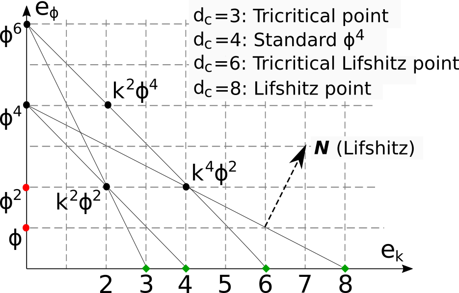
Figure 1: The exponent space for action integral (1) with model order $M=2$. A hyperplane represents a model with a critical point. Monomials on the upper right of a hyperplane are relevant for large wavevectors and irrelevant for small wavevectors. Monomials on the lower left of a hyperplane are relevant for small wavevectors and irrelevant for large wavectors.

This is shown for action (1) in fig.(1). Geometrically, equations (4) state that the exponents $E_{n,m}^{\left(0\right)}$ of marginal monomials can be interpreted as points on a hyperplane in a model-order dimensional exponent space. The hyperplane is orthogonal to the vector $\boldsymbol{N}$ of scaling dimensions. The critical dimensions $d_{c}$ together with the scaling dimensions $\boldsymbol{N}$ are a (not unique) signature for a scale invariant action integral.

To summarize, a scale invariance of an action integral requires selecting model oder monomials of the action integral. These monomials define a hyperplane in exponent space and determine the critical dimension and the scaling dimensions. It then may turn out that more (or even an infinite number of) monomials are consistent with the scale invariance.

3 Scaling below or above the critical dimension

The algebra decribed above must be extended to $d\neq d_{c}$ when the actual space dimension $d$ differs from the critical dimension $d_{c}$ or when dimensional regularization is to be used. Scale invariance is possible for $d\neq d_{c}$ if a coupling constant is assigned to one of the first $M$ monomials of the action integral. Which of the first $M$ monomials is assigned a coupling constant is more or less is a matter of taste.

The coupling constant then also gets a wave vector dimension and takes part in the scaling. The coupling constant adds a column to the exponent matrix and a row to the vector of scaling dimensions $\boldsymbol{N}$, but the first column of the exponent matrix and the value $N_{1}=1$ are known and can be moved to the r.h.s. of eq.(2). The $d$-dependent scaling dimensions then follow by inverting the resulting $M\times M$ matrix. The wavevector dimension of the coupling constant is of order $O\left(\epsilon\right)$, with $\epsilon=d_{c}-d$.

The resulting scale invariance of the action integral looks like a renormalization group flow for the coupling constant. This flow of coupling constants with a naive scaling dimension of order $O\left(\epsilon\right)$ is a part of the physical coupling constant flow, but has a physical meaning only when combined with the contribution from perturbation theory, which has the same order of magnitude.

No degrees of freedom are left once the $M\times M$-equation is solved, and in general all monomials after the first $M$ monomials need a coupling constant.

The software tool Kanon always determines the critical dimension and the canonical scaling dimensions from the first $M$ monomials of the action integral, and allows to shift monomials up and down by drag and drop.

Shifting monomials with a coupling constant of order $O\left(\epsilon\right)$ (marginal, on the same hyperplane) corresponds to arbitrary assignments in the renormalization scheme (which of the first $M$ vertex functions are kept fixed, which one of them has a coupling constant). The canonical dimensions in general change at order $O\left(\epsilon\right)$, but the physical scaling dimensions remain the same.

In contrast, when monomials with a coupling constant of order $O\left(1\right)$ (relevant or irrelevant, on a different hyperplane) are shifted to the first $M$ monomials, a different universality class (another hyperplane, or none at all) gets selected. See also fig.(1).

4 Dimensionless fields

The number of possible marginal monomials is finite as long as the hyperplane is not parallel to some field axis, i.e., as long as all scaling dimensions $\boldsymbol{N}$ differ from zero. It sometimes occurs that some field $\varphi_{m}$ is dimensionless, $\left[\varphi_{m}\right]=0$. Geometrically this means that the hyperplane is parallel to the field exponent axis, and that it intersects an unlimited number of lattice points (fig.(1)). Multiplying any marginal monomial of the action integral with any power of $\varphi_{m}$ generates another marginal monomial, and in principle an infinite set of monomials are marginal and must be taken into account.

The field theory and perturbative renormalization might still make sense. Some monomials might be forbidden by symmetry and not generated by perturbation theory. Or the perturbative expansion only involves these monomials step by step, and an iterative procedure is possible. But the situation always should be examined meticulously. Examples of field theories with a dimensionless field are nonlinear sigma models, the KPZ (Kardar, Parisi, Zhang) interface growth model, the Sine-Gordon model and the Wilson-Cowan neural network model.

5 Symmetries between fields

Some action integrals are symmetric under an exchange of two fields. An example is the Fermi action of beta decay[2]

$$S_{\mathrm{F}}=\int\mathrm{d}^{d}x\bar{\psi}\left(\gamma\cdot\partial+m\right)\psi+\left(\bar{\psi}\gamma\left(1-\gamma_{5}\right)\psi\right)\cdot\left(\bar{\psi}\gamma\left(1-\gamma_{5}\right)\psi\right).$$

The model order is three. The mass $m$ is irrelevant for large wavevectors, and there remain two monomials in $S_{F}$ - not enough to determine $d_{c}$, $\left[\psi\right]$ and $\left[\bar{\psi}\right]$. But because of the symmetry $\psi\leftrightarrow\bar{\psi}$ it suggests itself to require $\left[\psi\right]=\left[\bar{\psi}\right]$. This amounts to using only one field in the dimensional analysis, or to adding a constraint monomial $\bar{\psi}\psi^{-1}$ to $S_{F}$ (only for the scaling analysis, without any integrals!).

Any other constraint term like $\psi$ or $\bar{\psi}\psi^{3}$ not symmetric under the $\psi\leftrightarrow$$\bar{\psi}$ symmetry also does the job, even if this makes a field dimensionless. In fact, the two fields always occur in pairs, and only the sum of the dimensions $\left[\psi\right]+\left[\bar{\psi}\right]$ has physical meaning.

6 Field theories in wavevector space

In situations where a Fermi shell plays a role the field theory must be written down in $k$-space. Examples are the Fermi liquid with a four-point-interaction (superconductivity) and the Kondo effect. The algorithm used in Kanon for the dimensional analysis is oblivious to whether a “coordinate” denotes a coordinate or a wavevector. However, to get the correct sign for the scaling dimensions requires to set a flag for the coordinate. And of course, dimensions of fields and Fourier transforms of fields differ by the dimensions of the Fourier transform integrals.

7 Statistical physics and particle physics

With respect to scale invariance and the renormalization group there essentially is no difference between field theories of statistical physics and of particle physics. In the latter case the action occurs with a factor $i$ in the path integral, but this does not affect the essence of the renormalization group formalism.

The actual difference is the perspective. In statistical physics a system with atoms or molecules and usually a lattice is given, which defines an ultraviolett cutoff (UV), and one is interested in the behavior at decreasing wavevectors (long wavelengths, “infrared”, IR).

In partice physics the starting point is the physics at small wavevectors (low energy), and the question is how this came about or what will happen at high energies. Accordingly, one is interested in the behaviour for growing wavevectors.

A primitive example is the action $S=\int\mathrm{d}^{d}x\left(\left(\nabla\varphi\right)^{2}+m\varphi^{2}\right)$. The mass term $m\varphi^{2}$ dominates for small wavevectors (it is relevant) in comparison to $\left(\nabla\varphi\right)^{2}$, and this is what is of interest in statistical physics. In contrast, for large wavevectors (particle physics) the mass term is negligible (irrelevant). The difference only is the perspective.

8 Connection with the field theoretic renormalization group

Scale invariance of an action integral is a precondition for renormalizability, and a scaling analysis always should be the first step of a renormalization group calculation. The action integral must contain all types of marginal interactions, in particular if such interactions are generated by perturbation theory and/or are allowed by symmetry. If these preconditions are met, then renormalizibility is the rule rather than the exception.

The naive scaling at the level of the action integral contains the gist of scale invariance, but this exact classical symmetry is broken when fluctuations are taken into account (an example of an “anomaly”).

The actual scaling dimensions of the fields and coordinates and the flow of the coupling constants only follow from a renormalization group calculation. The field theoretic renormalization group is perturbative in nature, and gives reliable results only for small coupling constants. The corrections to the naive scaling then also are small. However complicated the calculations are, there remain a few typical possibilities.

8.1 At the critical dimension

In the vicinity of the trivial fixed point (with vanishing coupling constants) the renormalization group adds small logarithmic corrections to the naive scaling. If the fixed point is stable, then this in principle is the complete answer.

Examples are quantum chromodynamics with asymptotic freedom (UV stable trivial fixed point), or the standard $\varphi^{4}$-model in four dimensions with an IR-stable fixed point, or the Uniaxial magnet with dipolar interaction in three dimensions, also with a stable IR fixed point.

If the fixed point is unstable, then one knows the physics near the fixed point. But some coupling constant grows, and the ultimate behaviour away from the fixed point cannot be described with the pertubative renormalization group. Examples are quantum electrodynamics (UV unstable fixed point), quantum chromodynamics (IR unstable fixed point, confinement) and the Kondo effect also with an IR unstable fixed point. A Fermi liquid corresponds to an IR stable fixed point in any space dimension, but this fixed point is unstable under an attractive two-particle interaction (ultimately leading to superconductivity).

8.2 Below or above the critical dimension

Below (or sometimes above) the critical dimension $d_{c}$ an expansion parameter is $\epsilon=d_{c}-d$, and there may be fixed points of the coupling constant flow equations of order $O\left(\epsilon\right)$.

If there are stable fixed points for the coupling constants, then there are $\epsilon$-expansions for critical exponents and other quantities. This typically is the case in critical statics and critical dynamics, and for systems of the reaction-diffusion type (e.g. percolation).

If one is more interested in numerical values instead of in exact $\epsilon$-expansions, it also is possible to perform the renormalization group calculations directly in the given dimension $d$, and to expand quantities in the renormalized coupling constants (provided these are small in $d$ dimensions).

8.3 Non-renormalizable field theories

Quantum field theories are not renormalizable above their critical dimension.[3] Technically this means that there is a relevant interaction, and that the degree of divergence of diagrams for a vertex increases with the number of interactions. No finite number of subtractions renders the vertex finite. Such field theories still can make sense at tree level, as effective field theories. Examples are Fermi theory of weak interactions and Einstein-Hilbert gravitation[2], both with a critical (spacetime) dimension two.

9 Some special cases

There are some peculiar cases of renormalizable field theories, where a naive scaling analysis as described above can be misleading or somewhat involved.

9.1 Sine Gordon model

A monomial of the action integral can be strongly but dangerously irrelevant. This means that the monomial rapidly scales to zero according to naive scaling analysis (it is not on the hyperplane), but must be kept nevertheless. An example is the Sine-Gordon model[3] with action

$$S_{\mathrm{sg}}=\int\mathrm{d}^{d}x\left\{\left(\nabla\varphi\right)^{2}-\alpha\cos\varphi\right\}.$$

One of several pecularities of the Sine-Gordon model is that one coupling constant suffices for all powers of $\varphi^{2}$ in the $\cos\varphi$ series. The $\cos$-function can only play a role in this way if $\varphi$ is dimensionless. The first monomial then is marginal for $d=2$, while the $\cos\varphi$ would be marginal for $d=0$, but is strongly relevant in two dimensions.

A more standard version of the action contains an auxiliary field $\sigma$,

$$S_{\mathrm{sg}}^{\prime}=\int\mathrm{d}^{d}x\left\{\left(\nabla\varphi\right)^{2}-\lambda\sigma\cos\tfrac{\varphi}{2}+\tfrac{1}{2\gamma}\sigma^{2}\right\}.$$

Integrating out $\sigma$ from $e^{-S_{\mathrm{sg}}^{\prime}}$ leads back to $S_{\mathrm{sg}}$, but the monomials $\int\mathrm{d}^{d}x\sigma\varphi^{2n}$ now are marginal in two dimensions, the $\sigma^{2}$ is IR irrelevant. However, the $\sigma^{2}$ must be kept to be able to integrate over the auxiliary field $\sigma$. Calculations with action $S_{\mathrm{sg}}^{\prime}$ are not simpler than calculations with $S_{\mathrm{sg}}$. But the dimensional analysis is standard, and the first monomials of $S_{\mathrm{sg}}^{\prime}$ as usual define a hyperplane in exponent space (fig.(1)).

9.2 Kondo-effect

A system can be inhomogeneous in space and scale invariant. An example is the Kondo effect[4] with action integral

$$S_{\mathrm{Kondo}} =\int d\tau\int\mathrm{d}^{d}k\int\mathrm{d}\Omega\bar{\psi}\left(\partial_{\tau}+k\right)\psi+\int\mathrm{d}\tau\bar{\varphi}\partial_{\tau}\varphi$$

$$\qquad+\int\mathrm{d}\tau\left(\left(\int\mathrm{d}^{d}k\int\mathrm{d}\Omega\bar{\psi}\right)\boldsymbol{\sigma}\left(\int\mathrm{d}^{d}k\int\mathrm{d}\Omega\psi\right)\right)\cdot\left(\bar{\varphi}\boldsymbol{\sigma}\varphi\right)$$

The symbol $\tau$ denotes imaginary time, $\psi$ describes band electrons, $\varphi$ describes the defect electron at the origin. The action integral is written in $k$-space because of the Fermi surface for the band electrons. Components $\Omega$ of wavevectors parallel to the Fermi surface take not part in the scaling and only label the degrees of freedom (there is no distinguished $\Omega_{0}$ around which to scale $\Omega$). The symbol $k$ denotes the wavevector component perpendicular to the Fermi surface, and only $d=1$ has physical meaning. This is consistent with the critical dimension $d_{c}=1$ (this already indicates that the Kondo effect occurs in any space dimension $d_{\mathrm{space}}=d_{c}+\mathrm{dim}\left(\Omega\right)$). The nonlinear monomial is the interaction energy between band electrons and the defect electron, $\boldsymbol{\sigma}$ denotes the Pauli spin matrices (note that $\int\mathrm{d}^{d}k\int\mathrm{d}\Omega\psi\left(\boldsymbol{k}\right)=\psi\left(\boldsymbol{x}=0\right)$).

The action integral $S_{\mathrm{Kondo}}$ looks complicated, but the scaling analysis is pure formalism and accomplished in Kanon on the fly. The Pauli matrices $\boldsymbol{\sigma}$ and $\int\mathrm{d}\Omega$ are dimensionless and take not part in the scaling. As usual, once it is clear that $S_{\mathrm{Kondo}}$ is scale invariant, the way is open for a renormalization group calculation.

The fields $\varphi$ und $\bar{\varphi}$ actually only depend on imaginary time $\tau$ and thus are not fields in the usual sense. To remedy this one could write $\varphi=\Phi\left(\boldsymbol{x}=0\right)=\int\mathrm{d}^{d}k\int\mathrm{d}\Omega\Phi\left(\boldsymbol{k}\right)$ with a field $\Phi$. The scaling analysis also is standard with this notation. However, the two notations lead to hyperplanes with different normal vectors, i.e. the signatures differ. An advantage of the formulation with the $\Phi$-field might be, that insisting on using fields in the usual sense leads to a unique normal vector (signature) for the model.

10 Classification of renormalizible field theories, signature

As illustrated in fig.(1), renormalizable field theories are associated with hyperplanes in exponent space. Monomials on the hyperplane are marginal, monomials on one side are relevant, monomials on the other side are irrelevant.

Selecting different $M$ monomials from a set of monomials often selects different hyperplanes, and makes different monomials relevant, marginal or irrelevant.

This suggests to use the hyperplanes as signature for a critical model. A hyperplane contains at least model order linearly independent monomials. It can contain more monomials, all marginal and possibly important for the critical point. The correspondence is not unique, different universality classes can have the same hyperplane. For instance, the naive scaling analysis is the same for scalar und vector valued order parameters.

The signature consists of the critical dimension and the normal vector $\boldsymbol{N}=\left(\left[k_{m}\right];\left[\varphi_{m}\right]\right)$ of the hyperplane. The naive scaling dimensions $\left[k_{m}\right]$ and $\left[\varphi_{m}\left(\boldsymbol{x}\right)\right]$ can be arranged in increasing order, except for the first element $\left[k_{1}\right]=1$ for the $d$-dimensional space, which plays a special role. The table shows some examples

Name	Critical dimension	Signature
Directed percolation	4	$\left(1,2;2,2\right)$
Dynamical percolation	6	$\left(1,2;2,2,4,4\right)$
Model A of critical dynamics	4	$\left(1,2;1,3\right)$
Model J of critical dynamics	6	$\left(1,4;2,4\right)$
Gauge field theory	4	$\left(2;2,3,3\right)$
Fermi theory of weak interactions	2	$\left(2;1,1\right)$
Fermi liquid	1	$\left(2,2;1,1\right)$

Table 1: Signatures of some renormalizable field theories. “Critical dimension” here is the dimension of the $d$-dimensional space, not the some of all coordinate (and time) dimensions.

The vector element $N_{1}=1$ conveys no information, and it is possible to multiply $\boldsymbol{N}$ with the smallest integer converting all $N_{m}$ to integers. For action integrals formulated in wavevector space (instead of real space) the fields are functions of wavevectors, and Kanon calculates the dimensions of these fields. But to have an invariant signature one should use the dimensions of real space fields in the signature, which differ by the dimensions of the Fourier transform integrals. It also suggests itself to list coordinate dimensions (before the semicolon) and field dimensions (after the semicolon) in increasing order, except for the $d$-dimensional coordinate, which is the first element.

An interesting question is: how many renormalizable field theories are there for a given number of coordinates and a given number of fields? Exponents of fields in an action integral must be positive (the only known exception is conformal quantum mechanics).

Exponents of coordinates can be negative because of integrals (and sporadically inverse Laplace operators), but normally there is only one integral per coordinate (in real space).

If only a limited number of field factors and a limited number of derivates is allowed in each monomial, then the renormalizable field theories correspond to hyperplanes defined by $M$ monomials (points with integer coordinates) in some cuboid (or simplex) in $M$-dimensional exponent space (fig.(1)).

To find the hyperplanes defined by $M$ points with integer coordinates in this cuboid and other points on each hyperplane is a diophantine problem.

This problem can be attacked somewhat brute-force with the help of a computer, but not all hyperplanes lead to action integrals of the usual type. For instance, a hyperplane must contain monomials harmonic in the fields defining propagators, and more heuristic rules can be imposed. The mapping from a hyperplane to a renormalizable field theory is not unique, but it often is not difficult to write down plausible candidates. It would be of interest to classify all scale invariant action integrals for a given number of coordinates and fields and a given cuboid of exponents.

10.1 Additional marginal monomials

A related but simpler diophantine problem is to find all marginal monomials (in some range) of a given scale invariant action integral. This amounts to solving a linear diophantine equation. The structure of the solutions of linear diophantine equations is known[5]. There are $M-1$ linearly independent base vectors $e_{i}$, and the lattice $m_{0}+\sum n_{i}e_{i}$ with a marginal monomial $m_{0}$ and integers $n_{i}$ represents all marginal monomials.

Numerically, a simple brute-force search for additional marginal monomials in a cuboid of exponents turns out to be more efficient. The advantage of this approach is that the iterations run over exponents and that the iteration range has direct meaning. Kanon offers both algorithms.

In any case, one should check additional marginal monomials carefully. If such a monomial is generated in perturbation theory, then it must be taken into acount in renormalization group calculations.[6]

Many other marginal monomials can be ruled out by physical or formal reasons. If this is not the case, then adding the monomial to the action integral may convert it to another universality class. The question then is, whether the model with the additional interaction has a physical meaning.

11 Summary

The software tool Kanon offers a unified view on all types of renormalizable field theories. Action integrals can be defined interactively by drag and drop, and if an action integral turns out to be scale invariant, then what remains to be done is the renormalization group calculation.

When using the tool it should become clear, that a renormalizable field theory is associated with a hyperplane in an exponent space, determined by model order monomials. It should become clear that dimensionless fields are problematic, and it should become clear that it is to some degree arbitrary which monomials are kept fixed in the renormalization procedure, and which ones need a coupling constant. There often are additional marginal monomials, which can be determined in Kanon on the fly. Most of them can be ruled out by formal or physical reasons, but the other ones should be examined carefully.

The dimensional analysis of an action integral often is presented in the literature in concrete cases quite ad hoc with arguments of different quality. Scale invariance, however, is a precise mathematical concept, and having a tool for this purpose is useful for practical and didactic reasons.

References

- [1] R. Dengler, https://sourceforge.net/projects/kanon/, (2022).
- [2] M. D. Scadron, Advanced Quantum Theory, Springer, (1979).
- [3] J. Zinn-Justin, Quantum Field Theory and Critical Phenomena, Oxford science publications, (1997).
- [4] J. Kondo, Resistance minimum in dilute magnetic alloys, Progress of theoretical physics, 32(1), 37-49, (1964).
- [5] See, for instance: P. Bundschuh, Einführung in die Zahlentheorie, Springer (1991).
- [6] R. Dengler, Renormalization group calculation of the critical exponents for the Lifshitz tricritical point, Phys. Lett. 108A, 296(1985).