Enumeration of tree-type diagrams assembled from oriented chains of edges

Abstract

Using recurrent relations and an analog of the Lagrange inversion theorem, we obtain an explicit formula for the number of tree-type diagrams assembled with $k$ oriented labeled $q$-regular chains. Using a version of the Prüfer code for Cayley trees, we generalize our result to the case when the chains are not necessarily regular.

1 Statistical sum, cumulant expansion and diagrams

Let us consider a real symmetric $n$-dimensional matrix $A$ of the form

$$(A)_{ij}=\begin{cases}a_{ij},&\text{if $i\neq j$},\\ 0,&\text{if $i=j$,}\end{cases}\quad 1\leq i<j\leq n,$$

whose non-diagonal elements $a_{ij}$ are jointly independent Bernoulli random variables that take values 1 and 0 with probabilities $p$ and $1-p$. Then the family $\{A\}$ can be regarded as adjacency matrices of the Erdős-Rényi ensemble of random graphs with edge probability $p$ [2]. In paper [5], the following sum has been considered,

$$\Xi^{(n,\beta)}(g)={1\over(1+e^{-2\beta})^{n(n-1)/2}}\prod_{1\leq i<j\leq n}\ \sum_{{a_{ij}=0,1}}\exp\left\{-2\beta\sum_{1\leq i<j\leq n}a_{ij}+g\sum_{i,j=1}^{n}\left(A^{q}\right)_{ij}\right\}$$

that represents a mathematical expectation

$$\Xi^{(n,\beta)}(g)={\mathbb{E}}\exp\left\{gY_{q}^{(n)}\right\},\quad Y_{q}^{(n)}=\sum_{i,j=1}^{n}\left(A^{q}\right)_{ij}.$$

taken with respect to the measure generated by the ensemble of Erdős-Rényi random graphs with the edge probability $p=e^{-2\beta}/(1+e^{-2\beta})$.

Mathematical expectations of the form (3) can be viewed as discrete analogs of matrix integrals widely used in mathematical physics, where they are known as the matrix models of the quantum field theory (see, for example, monograph [1] and references therein). Asymptotic expansions of such integrals in the limit of infinite $n$ represent a source of large number of important results, in particular in combinatorics, including widely known map enumeration problems (see [1], chapter on random triangulations of surfaces and related topics).

It is known that the logarithm of the mathematical expectation of (3) developed into a formal series in powers of $g$ determines cumulants of the random variable $Y_{q}^{(n)}$,

$$f^{(n,\beta)}(g)=\log{\mathbb{E}}\exp\left\{gY_{q}^{(n)}\right\}=\sum_{k\geq 1}{g^{k}\over k!}Cum_{k}(Y^{(n)}_{q}).$$

One can study cumulants of the matrix product

$$Y^{(n)}_{q}=\sum_{i_{1},i_{q+1}=1}^{n}(A^{q})_{i_{1}i_{q+1}}=\sum_{i_{1},i_{2},\dots,i_{q+1}=1}^{n}a_{i_{1}i_{2}}a_{i_{2}i_{3}}\dots a_{i_{q}i_{q+1}}$$

with the help of a diagram technique, where a random variable $a_{i_{l}i_{l+1}}$ is associated with an edge that joins two vertices labeled by $i_{j}$ and $i_{l+1}$; the product $a_{i_{1}i_{2}}a_{i_{2}i_{3}}\dots a_{i_{q}i_{q+1}}$ is represented by an oriented chain ${\Lambda}^{(q)}$ that has $q+1$ vertices and $q$ edges. One can compute the $k$-th cumulant of $Y^{(n)}_{q}$ by considering a collection of $k$ chains ${\Lambda}_{1}^{(q)},\dots,{\Lambda}_{k}^{(q)}$, where equal random variables $a_{i_{l}i_{l+1}}$ are joined by an arc.

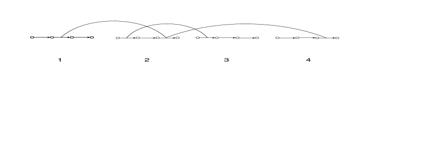
Figure 1: A diagram ${\cal D}_{4}^{(3)}$

It is shown in [5] that the leading term of the normalized cumulant of (4) in the limiting transition when $p=c/n$ and $n,c\to\infty$ is proportional to a number $d^{(q)}_{k}$ of connected diagrams ${\cal D}_{k}^{(q)}$ that have no cycles,

$${1\over nc}Cum_{k}\left({1\over c^{q}}Y^{(n)}_{q}\right)=2^{k-1}\ d^{(q)}_{k}(1+o(1)),\quad n,c\to\infty.$$

This means that $d_{k}^{(q)}$ is the number of multi-graphs with oriented edges obtained from the diagram of $k$ chains after identifying edges connected by an arc. Replacing the multi-edges by simple ones, we get a tree with $(q-1)k$ oriented edges. On Figure 1, we show an exemple of a connected tree-type diagram ${\cal D}_{k}^{(q)}$ with $q=3,k=4$.

The factor $2^{k-1}$ of (5) corresponds to signs $(+)$ and $(-)$ attributed to each arc. We assume that an arc has a sign $(+)$ when the edges glued have the same orientation and $(-)$ when they have the opposite direction. Everywhere below, we consider the diagrams with $(+)$-arcs only.

In the case of $q=2$, the following explicit formula is obtained in [5],

$$d^{(2)}_{k}=2^{k}(k+1)^{k-2},\quad k\in{\mathbb{N}}.$$

In this note we prove that for any integer $q\geq 2$,

$$d^{(q)}_{k}=q^{k}((q-1)k+1)^{k-2},\quad k\in{\mathbb{N}}.$$

It should be pointed out that sequence (6) is known as the number of trees with $k$ oriented labeled edges (see On-Line Encyclopedia of Integer Sequences [7], sequence A127670, and references given there). We did not found any reference to the sequence (7) with one or another value of $q$ and with or without the factor $q^{k}$, in the literature, including the open on-line sources. In particular, the sequence $\{d^{(3)}_{k}\}$ with $d^{(3)}_{0}=1$, $d^{(3)}_{1}=1$, $d^{(3)}_{2}=9$, $d^{(3)}_{3}=183$, $d^{(3)}_{4}=6561$, $d^{(3)}_{5}=323433,\dots$ is not presented in the OEIS [7].

2 Recurrence, Polya equation and Lagrange formula

In paper [5], it is shown that the following exponential generating function,

$$H_{q}(z)=\sum_{k\geq 0}{((q-1)k+1)\over k!}\,d_{k}^{(q)}z^{k}$$

verifies relation

$$H_{q}(z)=\exp\left\{qz(H_{q}(z))^{q-1}\right\}$$

known as the Pólya equation [8]. Equation (8) has been derived with the help of the recurrence procedure. For completeness, we repeat arguments of [5] to obtain recurrent relations for the numbers $d_{k}^{(q)}$.

Let us say that the edges of diagram ${\cal D}^{(q)}_{k}$ that are connected by arcs belong to the same color group. We also say that the edges of ${\cal D}^{(q)}_{k}$ that does not belong to any color group are grey edges. It is easy to see that if a diagram has $s$ color groups, then the number of grey edges in this diagram is equal to $(q-1)k-s+1$. Diagram ${\cal D}_{4}^{(3)}$ depicted on Figure 1 has two color groups and seven grey edges.

Let us consider the case when the next in turn chain ${\Lambda}^{(q)}_{k+1}$ is joined to a given diagram ${\cal D}^{(q)}_{k}$ by one arc only. The right foot of the arc can be put on one of $q$ edges of ${\Lambda}^{(q)}_{k+1}$ while there are $(q-1)k-s+1+s=(q-1)k+1$ possible emplacements given by on grey or on maximal color edges of ${\cal D}^{(q)}_{k}$ for the left foot to be put on.

To perform the general step of recurrence, we consider the case when there are $l$ arcs that join ${\Lambda}_{k+1}^{(q)}$ with other chains, $1\leq l\leq\min\{k,q\}$. We choose one of $\displaystyle{\displaystyle q\choose\displaystyle l}$ ways to put the right feet of arcs, choose $l$ subsets among $k$ elements of cardinality $j_{1},j_{2},\dots,j_{l}$ respectively such that $j_{1}+\dots+j_{l}=k$ and $j_{t}\geq 1$ and put the left feet of arcs to one of $(q-1)j_{t}+1$ possible emplacements of each diagram ${\cal D}_{j_{t}}^{(q)}$, $1\leq t\leq l$. We obtain the following relation,

$$d_{k}^{(q)}=\sum_{l=1}^{\min\{k,q\}}{q\choose l}\sum_{j_{1}+\dots+j_{l}=k,j_{i}\geq 1}\ {k!\over j_{1}!\cdots j_{l}!}\ \prod_{t=1}^{l}\big{(}(q-1)j_{t}+1\big{)}d_{j_{t}}^{(q)},\quad d_{1}^{(q)}=1.$$

Introducing auxiliary numbers $h_{j}^{(q)},j\in{\mathbb{N}}$,

$$h_{j}^{(q)}=\begin{cases}\big{(}(q-1)j+1\big{)}d^{(q)}_{j}/j!,&\text{if $j\geq 1$},\\ 1,&\text{if $j=0$,}\end{cases}$$

we deduce from (9) the following recurrent relation,

$$h_{k}^{(q)}={(q-1)k+1\over k}\ \sum_{j_{1}+\dots+j_{q}=k-1,j_{i}\geq 0}h_{j_{1}}^{(q)}\cdots h_{j_{q}}^{(q)},\quad k\geq 1.$$

Let us show that the generating function $H_{q}(z)=\sum_{k\geq 0}h_{k}^{(q)}\,z^{k}$ verifies (8). Indeed, assuming regularity of $H_{q}(z)$ one can easily deduce from (10) relation

$$H_{q}(z)-1=z(q-1)\big{(}H_{q}(z)\big{)}^{q}+\int_{0}^{z}\big{(}H_{q}(\zeta)\big{)}^{q}d\zeta$$

that is equivalent to the differential equation

$${dH_{q}(z)\over dz}={q(H_{q}(z))^{q}\over 1-q(q-1)z(H_{q}(z))^{q-1}}$$

(we will see below that $H_{q}(z)$ is analytic in the domain $\{z\in{\mathbb{C}}:|z|<{1/(q(q-1)e)}\}$). Substitution

$$\psi(z)=z(H_{q}(z))^{q-1}$$

transforms (11) to an equation

$$z\psi^{\prime}(z)={\psi(z)\over 1-q(q-1)\psi(z)}.$$

Resolving this equation with obvious initial condition, we conclude that $\psi(z)$ verifies the Pólya equation

$$\psi(z)=ze^{q(q-1)\psi(z)}.$$

Then (8) follows from (12) and (13). Let us note that equation (13) is known in combinatorics an equation for the exponential generating function of Cayley trees.

Using equation (8), one can obtain explicit expressions for the coefficients $H^{(q)}_{k}$. In the case of $q=2$, this has been done in paper [5] with the help of the contour integration method of the Lagrange inversion theorem [6]. Here we give the answer in the general case $q\geq 2$.

Let us consider a function

$$t(w)=we^{-q(q-1)w},\quad w\in{\mathbb{C}}$$

that is analytic in a vicinity of zero with the derivative non-zero in the domain $\{w\in{\mathbb{C}}:|w|<(q(q-1))^{-1}\}$ and has its inverse $t^{-1}(z)=\psi(z)$. Then $\psi(z)$, $z\in{\mathbb{C}}$ is also analytic in a vicinity of zero. The same is true for

$$H_{q}(z)=e^{q\psi(z)}=\sum_{k=0}^{\infty}C_{k}z^{k},$$

where the series converges and where $C_{k}=h_{k}^{(q)}$. Then we can write that

$$C_{k}={1\over 2\pi i}\oint{e^{q\psi(z)}\over z^{k+1}}\,dz.$$

Taking into account (13), relation $z=t(w)$ and equality

$$dz=\left(e^{-q(q-1)w}-q(q-1)we^{-q(q-1)w}\right)\,dw$$

that follows from (14), we rewrite (15) in the form

$$C_{k}={1\over 2\pi i}\oint{e^{qw+q(q-1)wk}\over w^{k+1}}\left(1-q(q-1)w\right)dw$$

$$=\lfloor e^{q(q-1)wk+qw}\rfloor_{(k)}-q(q-1)\lfloor e^{q(q-1)wk+qw}\rfloor_{(k-1)},$$

where we denoted by $\lfloor f(w)\rfloor_{(k)}$ the $k$-th coefficient of the Taylor expansion of $f(w)$ at zero. Then

$$h^{(q)}_{k}={q^{k}\over k!}\big{(}(q-1)k+1\big{)}^{k-1}-{q^{k}(q-1)\over(k-1)!}\big{(}(q-1)k+1\big{)}^{k-1}={q^{k}\over k!}\big{(}(q-1)k+1\big{)}^{k-1}.$$

Remembering definition of $h^{(q)}_{j}$, we get the final expression for $d_{k}^{(q)}$ (7).

3 Prüfer code for rooted tree-type diagrams

The right-hand side of (7) clearly refser to the tree structure of the diagrams we study and assumes existence of its direct combinatorial proof. In this section, we develop a version of the Prüfer code to prove (7). The Prüfer code has been developed to prove the Cayley formula for the number of free trees on $k$ vertices (see for instance [4]). There exists a waste literature concerning the use of the Prüfer code and its generalizations. In particular, it can be used also to obtain the number of trees with $k$ oriented labeled edges [3] with the help of the Cayley formula. What we do here resembles the reasoning of [3] with a version of the Prüfer code developed directly for the rooted trees with $k$ labeled edges (see [3], Lemma 2 and its proof). One could also trace out a relation with the paper [4], where the Prüfer code has been developed for the number of connected graphs assembled with $k$ blocks. However, the difference is that in our case the vertices of blocks cannot be labelled in arbitrary way.

The chain elements we considered above can be associated with cycles of $q$ edges with one marked vertex and an orientation attributed to this cycle, so the edges of the cycle can be regarded as the oriented and ordered ones. We denote by $\lambda_{i}$ the cycles obtained. The arcs of a diagram ${\cal D}_{k}^{(q)}$ indicate the edges to be glued together. Applying this procedure to the cycles $\lambda_{i}$, we obtain a tree-type diagram ${\cal T}_{k}^{(q)}$ that represents a connected graph with multiple edges. We say that $\lambda_{i}$ are cycle elements of ${\cal T}^{(q)}_{k}$. On figure 2, we depict such a tree-type diagram ${\cal T}_{4}^{(3)}$ obtained from the diagram ${\cal D}_{k}^{(q)}$ shown on figure 1.

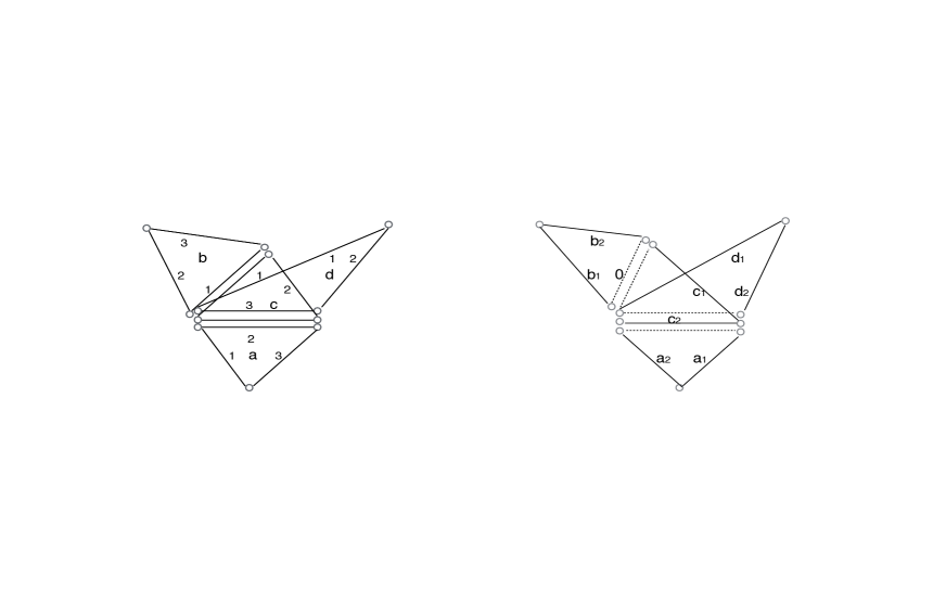
Figure 2: A tree-type diagrams ${\cal T}_{4}^{(3)}$ and $\tilde{\cal T}_{4}^{(3)}$

We assume elements $\lambda_{1},\lambda_{2},\dots,\lambda_{k}$ to be colored in $k$ different colors; these colors are ordered, say $(a,b,c,\dots,h)$; all edges of $\lambda_{i}$ are colored with the same color. To get the Prüfer code, the diagram is modified by the following procedure:

1) choose a couple of vertices of ${\cal T}_{k}^{(q)}$ that are connected by a simple or multiple edge; wash out the colors of all simple edges it has and consider this (multi)edge as the root one; all edges of the elements $\lambda_{i}$ attached to this root edge keep their colors they have; we say that these edges are dominant;

2) consider an element $\lambda_{j}$ attached to one of the dominant edges and wash out the color of the edge of $\lambda_{j}$ attached to the dominant edge; all other edges of $\lambda_{j}$ keep their color and are included to the list of the dominant edges;

3) repeat this action as many times as possible. After this procedure performed, each edge of an element $\lambda_{i}$ is colored excepting the one that we call the bottom edge of $\lambda_{i}$. The diagram obtained $\hat{\cal T}_{k}^{(q)}$ counts $(q-1)k$ colored edges.

4) the left vertex of the bottom edge of each element $\lambda_{j}$ is announced to be the marked vertex; we order the color edges of the same element by labeling them with subscripts in the clockwise direction, say $a_{1},a_{2},\dots,a_{q-1}$. The step (4) being performed, we get a diagram $\tilde{\cal T}_{k}^{(q)}$. On Figure 2 we depict the diagram $\tilde{\cal T}_{4}^{(3)}$ obtained from ${\cal T}_{4}^{(3)}$. Here the edges with the color washed out are represented by dotted lines. The root edge is marked by ”0”.

Given such a prepared diagram $\tilde{\cal T}_{k}^{(q)}$, we can write down the Prüfer code by the standard procedure known for the trees: $\alpha$) find the minimal color such that there is no other element of ${\cal T}_{k}^{(q)}$ attached to the element $\lambda^{\prime}$ of this color;

$\beta$) write down the color with subscript of the edge that $\lambda^{\prime}$ is attached to; in the case when the element $\lambda^{\prime}$ has a root edge, write down ”0” instead of the color with subscript;

$\gamma$) erase the element $\lambda^{\prime}$ from the diagram ${\cal T}_{k}^{(q)}$ and denote the diagram obtained by $\tilde{\cal T}_{k-1}^{(q)}$;

$\delta$) perform the steps $(\alpha),(\beta)$ and $(\gamma)$ to obtain $\tilde{\cal T}_{k-2}^{(q)}$, then $\tilde{\cal T}_{k-3}^{(q)}$ and so on. We repeat the procedure of $(\delta)$ till the last step number $k-1$ is performed. On this stage the diagram $\tilde{\cal T}_{1}^{(q)}$ contains only one element that contains the root edge. Thus we get a sequence of $k-1$ cells (windows) with letters with subscript therein; we denote this Prüfer-type sequence by ${\cal P}_{k-1}^{(q)}$. In each window one can see one of $(q-1)k+1$ values, therefore there are $((q-1)k+1)^{k-1}$ different sequences like this.

For example, regarding the diagram ${\cal T}_{4}^{(3)}$ depicted on Figure 3, we get the following Prüfer sequence:

$${\cal P}_{3}^{(3)}=\begin{tabular}[]{|c|c|c|c|}$c_{2}$&$0$&$c_{2}$\\ \hline\cr\end{tabular}$$

The inverse procedure is very similar to that of the original Prüfer code: - we start by writing down a Prüfer-type sequence ${\cal P}_{k-1}^{(q)}$; under ${\cal P}_{k-1}^{(q)}$ we write down a line ${\cal L}_{k}$ of the values $a,b,c,\dots,h$; we say that $({\cal P}_{k-1}^{(q)},{\cal L}_{k})$ represents the color Prüfer code;

i) in ${\cal L}_{k}$, we underline all letters that appear in ${\cal P}_{k-1}^{(q)}$;

ii) we take the value of the first window of ${\cal P}_{k-1}^{(q)}$ that we denote by $w_{1}$ and find the first value from the line ${\cal L}_{k}$ that is not underlined, say $r$; then we join the element colored by $r$ to the edge indicated by $w_{1}$; erasing $w_{1}$ and the first window from ${\cal P}_{k-1}^{(q)}$ and erasing $r$ from ${\cal L}_{k}$ we get the color Prüfer code $(P_{k-2}^{(q)},{\cal L}_{k-1})$.

Repeating the steps (i) and (ii) till the obvious $k$-th step when the last element from the line ${\cal L}_{1}$ that has the root edge $0$, we get the diagram $\tilde{\cal T}^{(q)}_{k}$ that has been encoded by the Prüfer sequence ${\cal P}^{(q)}_{k-1}$.

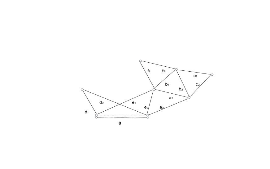
Figure 3: A tree-type diagram $\tilde{\cal T}_{6}^{(3)}$

For example, given a color Prüfer code $({\cal P}_{5}^{(3)},{\cal L}_{6})$ as follows,

$${\cal P}_{5}^{(3)}$$ 0

a b c d e f

where the last boldface zero of the first line is added for convenience as a muet variable always equal to $0$, we get the diagram $\tilde{\cal T}_{6}^{(3)}$ depicted on Figure 3. For simplicity, we do not present the dotted bottom edges, excepting the dotted root edge marked by ”0”. We see that one can split the construction of $\tilde{\cal T}_{6}^{(3)}$ in the following steps:

$$c\mapsto b_{2},\quad d\mapsto 0,\quad f\mapsto b_{1},\quad b\mapsto a_{1},\quad a\mapsto e_{2},\quad e\mapsto{\bf 0}.$$

It is clear that each $\tilde{\cal T}^{(q)}_{k}$ generates a unique Prüfer sequence ${\cal P}_{k-1}^{(q)}$ and each Prüfer sequence ${\cal P}_{k-1}^{(q)}$ represents a unique tree-type diagram of the form $\tilde{\cal T}_{k}^{(q)}$. On this way, we obtain $((q-1)k+1)^{k-1}$ rooted diagrams. Eliminating the choice of the root edge, we divide the number of rooted diagrams by $(q-1)k+1$. Rotating the special marked vertex of each element in ${\cal T}_{k}^{(q)}$, we get the factor $q^{k}$. This gives (7).

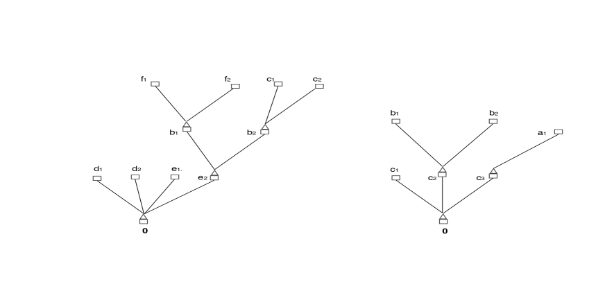
Figure 4: A regular tree diagram $\tilde{\Gamma}_{6}^{(3)}$ and irregular tree diagram $\tilde{\Gamma}^{(1,2,3)}_{3}$

We can see from the last graphical representation that elements $\lambda_{i}$ of the diagram ${\cal T}_{k}^{(q)}$ can also be represented as a kind of stars that have $q-1$ edges attached to the vertex that we denote by triangles; we denote the end vertices of these edges by rectangles. The rectangle vertices can be used as a base for the triangle vertices to be put on. Then we get a tree diagram $\tilde{\Gamma}_{k}^{(q)}$. On Figure 4 we present $\tilde{\Gamma}^{(3)}_{6}$ that corresponds to $\tilde{\cal T}^{(3)}_{6}$ from Figure 3. Then the analogy of the tree-type diagrams ${\cal T}_{k}^{(q)}$ and trees becomes even more clear that before. This representation can be especially useful in the case of $q=2$, when $\Gamma_{k}^{(2)}$ represents a classical tree with $k$ oriented edges. This representation gives a direct combinatorial explanation of the formula (6) [3, 5].

Let us note that the Prüfer-type code developed above to prove (7) can be generalized to the case of tree-type diagrams ${\cal D}^{(q_{1},\dots,q_{k})}_{k}$ whose elements ${\Lambda}_{1},\dots,{\Lambda}_{k}$ have $q_{1},\dots,q_{k}$ edges, respectively. On Figure 4 we present an exemple of an irregular tree diagram $\tilde{\Gamma}^{(1,2,3)}_{3}$ that gives the Prüfer sequence $(c_{3},c_{2})$. It is easy to see that the number of such non-regular tree diagrams $\Gamma_{k}^{(q_{1},\dots,q_{k})}$ is given by the following expression,

$$d^{(q_{1},\dots,q_{k})}_{k}=\big{(}(q_{1}+\dots+q_{k})(k-1)+1)^{k-2}\ \prod_{i=1}^{k}q_{i}\ .$$

It is not clear for us whether (16) leads to a kind of Polya equation of the form (8) or (13).

References

- [1] J. Ambjorn, B. Durhuus, Th. Jonsson, Quantum Geometry: A Statistical Field Theory Approach, Cambridge University Press, 1997
- [2] B. Bollobaś, Random Graphs, Cambridge University Press, 2001
- [3] R. Barequet, G. Barequet, G. Rote, Formulae and growth rates of high-dimensional polycubes, Combinatorica, 30 (2010), no. 3, 257?275
- [4] H. Kajimoto, An extension of the Prüfer code and assembly of connected graphs from their blocks, Graphs Combin. 19 (2003) 231-239
- [5] O. Khorunzhiy, On connected diagrams and cumulants of Erdős-Rényi matrix models, Commun. Math. Phys. 282 (2008) 209-238
- [6] Pólya, George; Szegö, Gabor Problems and theorems in analysis. I. Series, integral calculus, theory of functions, Reprint of the 1978 English translation. Classics in Mathematics. Springer-Verlag, Berlin, 1998. xx+389 pp
- [7] The on-line encyclopedia of integer sequences, https://oeis.org
- [8] R. P. Stanley, Enumerative combinatorics, Vol. 2, Cambridge Studies in Advanced Mathematics, 62 Cambridge University Press, Cambridge, 1999. xii+581 pp