DRESS: Dynamic REal-time Sparse Subnets

Abstract

The limited and dynamically varied resources on edge devices motivate us to deploy an optimized deep neural network that can adapt its sub-networks to fit in different resource constraints. However, existing works often build sub-networks through searching different network architectures in a hand-crafted sampling space, which not only can result in a subpar performance but also may cause on-device re-configuration overhead. In this paper, we propose a novel training algorithm, Dynamic REal-time Sparse Subnets (DRESS). DRESS samples multiple sub-networks from the same backbone network through row-based unstructured sparsity, and jointly trains these sub-networks in parallel with weighted loss. DRESS also exploits strategies including parameter reusing and row-based fine-grained sampling for efficient storage consumption and efficient on-device adaptation. Extensive experiments on public vision datasets show that DRESS yields significantly higher accuracy than state-of-the-art sub-networks.

1 Introduction

There is a growing interest to deploy deep neural networks (DNNs) on resource-constrained edge devices to enable new intelligent services such as mobile assistants, augmented reality, etc. However, state-of-the-art DNNs often make significant demands on memory, computation, and energy. Extensive works [9, 28, 5, 8] have proposed to first compress a pretrained model given resource constraints, and then deploy the compressed model for on-device inference.

However, the time constraints of many practical embedded systems may dynamically change at run-time, e.g. detecting hand position with different speed in real-time, autonomous vehicles’ reaction time on city roads and highways. On the other hand, the available resources on a single device may also vary, e.g. the battery energy, the amount of allocatable RAM. All these considerations indicate that the deployed inference model should maintain a dynamic capacity to be executed under different resource constraints.

Making DNNs adaptable on resource-constrained edge devices is even more challenging. Existing works either fail to adapt to different resource constraints, or result in a subpar performance. Traditional compression techniques, e.g. pruning, quantization, only result in a static inference model. Although the compressed model is well-optimized and deployed on edge devices, it can not meet various resource requirements. As an alternative, we may deploy for example multiple networks with different sparsity levels [35, 22], which however need several times more storage consumption in comparison to a single sparse network. Recent works [37, 4] show that the sub-networks from a pretrained backbone network can reach a decent performance compared to the sub-networks trained individually from scratch. Nevertheless, they only sample the sub-network architectures along hand-crafted structured dimensionalities, e.g. width, kernel size, which leads to sub-optimal results. Switching among different architectures in run-time may also cause extra re-configuration overhead.

In this paper, we propose Dynamic REal-time Sparse Subnets (DRESS). DRESS samples sub-networks from the backbone network through row-based unstructured sparsity, while ensuring that nonzero weights of the higher sparsity networks are reused by the lower sparsity networks. This way, the overall memory consumption is bounded by the network with the lowest sparsity and does not depend on the number of networks, resulting in memory efficiency; all sparse sub-networks leverage the same architecture as the backbone network, leading to re-configuration efficiency. The sub-network with a higher sparsity (i.e. fewer nonzero weights) needs a smaller amount of on-device memory fetching and fewer multiply-accumulate operations (FLOPs), thus shall be adopted to inference under more severe resource constraints, e.g. lower energy budget, limited inference time.

Specifically, we (i) sample weights w.r.t. their magnitudes in a row-based fine-grained manner; (ii) train all sampled sparse sub-networks with weighted loss in parallel; (iii) further fine-tune batch normalization for each sub-network individually. Our contributions are summarized as,

• We design a training pipeline DRESS that generates multiple sub-networks from the backbone network with weight sharing.

• We propose a row-based fine-grained sampling that allows subnets to be efficiently stored and executed using our proposed compressed sparse row (CSR) format.

• Experimental results show DRESS reaches a similar accuracy while only requiring 50%-60% disk storage as unstructured pruning.

2 Related Works

Network compression & deployment. Network compression focuses on trimming down the DNN model size. Commonly used compression techniques consist of, (i) designing efficient network architectures manually [14, 31] or automatically [13, 33, 4]; (ii) quantizing weight into lower bitwidth [5, 28, 27]; (iii) structured [22, 20]/unstructured [9, 8, 29, 7, 25] pruning unimportant weights as zeros to reduce the number of operations (also compute energy) and the number of nonzero weights (also memory consumption). The compressed model is further optimized by some libraries to speed up inference on certain edge platforms, e.g. XNNPACK for ArmV7 CPU [1]. Note that the optimized model often only supports a static computation graph due to the limited resources on edge devices [18, 1, 2]. We focus on unstructured pruning, since (i) it often yields a higher compression ratio [29]; (ii) the networks with different unstructured sparsity may share the same network architecture, i.e. the same computation graph. Furthermore, the recently released XNNPACK library includes fast kernels for sparse matrix-dense matrix multiplication, which enables sparse DNN acceleration on edge platforms [6].

Dynamic networks and anytime networks. Dynamic networks and anytime networks aim at an efficient inference through adapting network structures. Dynamic networks [10, 15, 21, 34] realize an input-dependent adaptation to reduce the average resource consumption during inference. Unlike dynamic networks, anytime networks refer to the network whose sub-networks can be executed separately under a resource constraint while achieving a satisfactory performance. DRESS falls into the same scope of anytime networks. MSDNet [15] densely connects multiple convolutional layers in both depth direction and scale direction, such that the computation can be saved by early-exiting from a certain layer. Slimmable networks [37, 36] propose to train a single model which supports multiple width multipliers (i.e. number of channels) in each layer. Subflow [19] executes only a sub-graph of the full DNN by activating partial neurons given the varied time constraints. State-of-the-art anytime networks always sample sub-networks from the backbone network along hand-crafted structured dimensionalities, e.g. depth, width, kernel size, neuron. As zero weights have no effects on the calculation, anytime networks actually perform structured pruning on the backbone network, which could result in a subpar performance in comparison to unstructured sampling. In addition, resulted sub-networks often have different architectures, e.g. different kernel sizes, the re-configuration of the computation graph may bring extra overhead during on-device adaptation.

3 Dynamic Real-time Sparse Subnets

Problem Definition We aim at sampling multiple subnets from a backbone network. The backbone network is a traditional DNN consisting of $L$ convolutional (conv) layers or fully connected (fc) layers. To achieve memory efficiency, the nonzero weights of the subnet with a higher sparsity are reused by the subnet with a lower sparsity. This way, we only need to store a table for the lowest sparsity network, including its nonzero weights sorted w.r.t. importance and corresponding indices. Accordingly, the other networks can be built from the top important weights through a pre-defined sparsity level. Assume that we sample altogether $K$ sparse subnets, then the preliminary problem is defined as,

$$\min_{\bm{w},\bm{m}_{k}} \mathcal{L}(\bm{w}\odot\bm{m}_{k}) \forall k\in 1...K$$ (1)

s.t. $$\|\bm{m}_{k}\|_{0}=(1-s_{k})\cdot I \forall k\in 1...K$$ (2)

$$\bm{m}_{i}\odot\bm{m}_{j}=\bm{m}_{j} \forall 1\leq i<j\leq K$$ (3)

where $\bm{w}$ stands for the weights of the (dense) backbone network; $\bm{m}_{k}$ stands for the binary mask of the $k$-th subnet; $s_{k}$ stands for the pre-defined sparsity level. $\mathcal{L}(.)$ denotes the loss function, $\|.\|_{0}$ denotes the L0-norm, $\odot$ denotes the element-wise multiplication. Note that $\bm{w}\in\mathbb{R}^{I}$, $\bm{m}_{k}\in\{0,1\}^{I}$, where $I$ is the total number of weights. We have $0<s_{1}<...<s_{K}\leq 1$. $\bm{w}_{k}$ is denoted as nonzero weights of the $k$-th sparse subnet, i.e. $\bm{w}_{k}=\bm{w}\odot\bm{m}_{k}$.

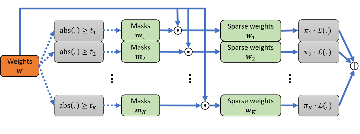
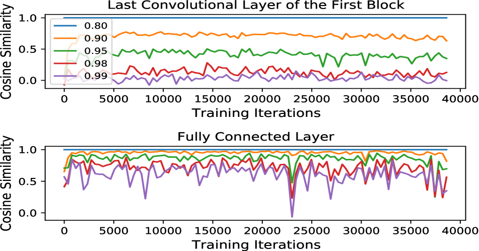
Figure 1: Left: The computation graph used in parallel training multiple subnets. The orange blocks are the leaf variables to be optimized; the green blocks are the intermediate variables; the gray blocks are the computation units. The solid arrows are the differentiable operation to be backpropagated, but the dashed arrows are not. Right: The cosine similarity between the loss gradients of 5 subnets (with sparsity 0.8,0.9,0.95,0.98,0.99) and that of the lowest sparsity subnet with sparsity 0.8. We show two typical layers in ResNet20.

In the following sections, we detail how to solve Eq.(1)-Eq.(3) in our DRESS algorithm. DRESS consists of three training stages, (i) dense pre-training, where the backbone network is trained from scratch to provide a good initial point for the following sparse training; (ii) DRESS training, where multiple sparse subnets are sampled from the backbone network (Sec. 3.1, Sec. 3.3) and are jointly trained in parallel with weighted loss (Sec. 3.2); (iii) post-training on batch normalization (BN), where BN layers are further optimized individually for each subnet to better reveal the statistical information, as BN layers often require a rather small amount of memory and computation. The overall pseudocode is shown in Alg. 1 in Appendix A.

3.1 How to Sample Sparse Subnets

Unlike traditional anytime networks that sample subnets along structured dimensionalities, DRESS samples subnets weight-wise which extremely enlarges the sampling space. The naive approach could be iteratively sampling $K$ subnets by exhaustively searching the best-performed subnet inside the current subnet. However, it can be either conducted rarely or infeasible due to the high complexity. To reduce the complexity, we propose to greedily sample the subnets based on the importance of weights. As previous pruning works [9, 8, 29], the importance of weights is measured by their magnitudes. Given an overall sparsity level $s_{k}$, the $(1-s_{k})\cdot I$ weights with the largest magnitudes will be sampled to build the subnet. To further reduce the sorting complexity, the weights are only sorted inside each layer according to a layer-wise sparsity $s_{k,l}$, where $l$ denotes the layer index. The global sorting, also the (re-)allocation of layer-wise sparsity, is conducted only if the average accuracy of subnets does not improve anymore, see Alg. 1. During (re-)allocation, the weights of all layers with the largest magnitudes are selected in sequence until reaching the overall sparsity $s_{k}$, and the layer-wise sparsity can be then calculated accordingly.

3.2 How to Optimize Subnets

With sampled binary masks, we can now build and train the subnets. Our concept for optimizing subnets is based on the key insight: in comparison to iterative training of subnets in progressively decreased/increased sparsity, parallel training allows multiple subnets to be sampled and optimized jointly, which avoids being stuck into bad local optimum and thus yields higher performance. Experimental results in Appendix C.1 verify that parallel training yield significantly higher performance than iterative training. In parallel training, Eq.(1) can be re-written as,

$$\min_{\bm{w},\bm{m}_{k}}~{}~{}~{}\sum_{k=1}^{K}\pi_{k}\cdot\mathcal{L}(\bm{w}\odot\bm{m}_{k})\vspace{-0.5em}$$ (4)

where $\pi_{k}$ is the normalized scale ($\sum_{k=1}^{K}\pi_{k}=1$) used to weight $K$ loss items, which will be discussed later. This process determines a threshold $t_{k}$, the mask value $m_{k,i}=1$ if $\mathrm{abs(}w_{i}\mathrm{)}\geq t_{k}$, otherwise 0, $\forall i\in 1...I$. $t_{k}$ is set to the value such that $(1-s_{k})$ of weights have a larger absolute value than $t_{k}$. Clearly, we have $t_{1}<t_{2}<...<t_{K}$ due to the constraints of Eq.(2)-Eq.(3). In each training iteration, we sample $K$ sparse subnets $\bm{w}_{1:K}$ and optimize the backbone $\bm{w}$ with the weighted sum of their losses, see in Fig. 1 Left.

We parallelly train 5 subnets of ResNet20 [11] on CIFAR10, and let 5 loss items weighted equally, i.e. $\pi_{1:5}=0.2$. We plot the cosine similarity between the loss gradients (i.e. $(\partial\mathcal{L}(\bm{w}_{k})/\partial\bm{w}_{k})\odot\bm{m}_{k}$) of 5 subnets and that of the lowest sparsity subnet along with the training iterations, see in Fig. 1 Right. It shows that the loss gradients of different subnets are always positively correlated, which also verified that multiple subnets are jointly trained towards the optimal point in the loss landscape. Because of Eq.(3), the nonzero weights in higher sparsity subnets are also selected by other subnets, which means these weights are optimized with a larger step size than others. To balance the step size, we propose to weight the loss items by the ratio of trainable weights (i.e. $1-s_{k}$) together with a correction factor $\gamma$. Particularly, $\alpha_{k}=(1-s_{k})^{\gamma}$, and with the normalization, $\pi_{k}=\alpha_{k}/\sum_{k=1}^{K}\alpha_{k}$. Note that $\gamma=0$ means weighting loss items equally. Experimentally, we find that $\gamma=0.5$ often yields a satisfactory performance, see Appendix C.2.

3.3 How to Store Subnets

State-of-the-art libraries often encodes sparse tensor in compressed sparse row (CSR) format for sparse inference [1, 6]. To achieve an efficient inference on different sparse subnets while without extra memory overhead, we adopt a row-based unstructured sparsity, where different rows leverage the same sparsity level. Especially, for sparsity $s_{k}$, all rows have exactly $(1-s_{k})\cdot N$ nonzero weights, where $N$ is the number of weights per row. In comparison to conventional unstructured sparsity, this kind of sparsity (a.k.a. N:M fine-grained structure sparsity [38, 16, 32]) can also be accelerated with sparse tensor cores of A100 GPUs [23] for both training and inference, and thus becomes prevailing recently. The column indices of nonzero weights are stored in descending order of the importance (also the weight magnitude) in a two-dimensional table. The nonzero weights are stored in a table with the same order as the column indices. This DRESS CSR format needs to store (i) the subnet with the lowest sparsity including the table of the column indices and the table of nonzero weights, (ii) $K$ integers $\{(1-s_{k})\cdot N\}_{k=1}^{K}$. When adopting the $k$-th subnet, we fetch the first $(1-s_{k})\cdot N$ columns from both tables as shown in Fig. 2. Note that all fetched subnets follow the CSR format ($(1-s_{k})\cdot N$ is used to build the row indices in CSR) under the same architecture, which allows us to leverage available libraries to achieve a fast on-device inference without re-configuration overhead. To obtain DRESS CSR format, the sampling process needs to be adjusted accordingly. Especially, for layer $l$, we first pre-define a row size $N_{l}$ and reshape the weight tensor into rows. In this paper, the weights corresponding to each output channel (e.g. each conv filter) are formed into one row. The row-based sampling is shown in Alg. 4 in Appendix A.3.

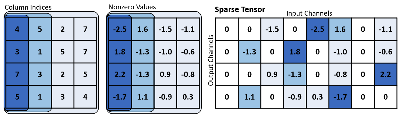
Figure 2: DRESS CSR format of row-based unstructured sparse tensor. The example weight tensor is from a $1\times 1$ conv layer with 8 input channels and 4 output channels. Each row has 8 weights in total, also the row size $N=8$. There are 3 sparse subnets with sparsity 0.5, 0.75, and 0.875. Each subnet has 4, 2, and 1 nonzero weights per row, respectively.

4 Experiments

We implement DRESS with Pytorch [24], and evaluate its performance on CIFAR10 [17] using ResNet20 [11], on ImageNet [30] using ResNet50 [11]. We randomly select 20% of each original test dataset (original validation dataset for ImageNet) as the validation dataset, and the remainder as the test dataset. We use the Nesterov SGD optimizer with the cosine schedule for learning rate decay in all methods. We report the Top-1 test accuracy for the subnets of the epoch when the validation dataset achieves the highest average accuracy over all subnets. More implementation details are provided in Appendix B. Row-based unstructured sampling is conducted in all layers except for BN layers. We set the sparsity levels $s_{1:5}=0.8,0.9,0.95,0.98,0.99$ for ResNet20, and $s_{1:4}=0.5,0.8,0.9,0.95$ for ResNet50.

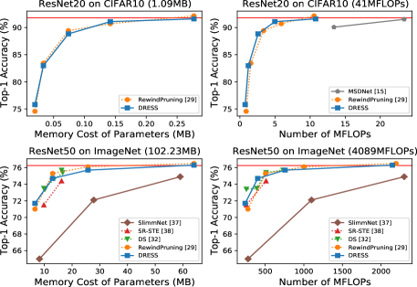
Figure 3: Comparing DRESS with other baselines. The methods that do not involve weight sharing among different networks are plotted with dotted curves. The memory cost and the number of MFLOPs of the original backbone networks are reported in the parentheses in titles; their accuracy is shown as red horizontal lines.

We compare the performance of the subnets generated by DRESS with various methods, including (i) anytime networks [15, 37], where the sub-networks with different width or depth can be cropped from the backbone network; (ii) unstructured pruning [29], where the backbone network is pruned with the same sparsity as DRESS; (iii) N:M fine-grained structure pruning [38, 32]. We choose two metrics for comparison, the memory cost of parameters and the number of FLOPs. FLOPs dominate in the entire computation burden, thus fewer FLOPs can (but does not necessarily) result in a smaller computation time. The memory cost of parameters represents not only the disk storage consumption but also the amount of memory fetching during on-device inference. Note that memory access often consumes more time and energy than computation [12]. Assume that each weight uses 32-bit floating point. DRESS, (ii), and (iii) generate sparse tensors, thus their memory cost also includes the indices of nonzero weights. Each index of nonzero weights are encoded into 8-bit in DRESS and (ii) as [3, 1], wheres the binary mask is stored for indexing in [38, 32].

The results are plotted in Fig. 3. DRESS require a significantly lower memory cost and fewer FLOPs than other anytime networks. Furthermore, different subnets of DRESS leverage the same architecture as the backbone network, which avoids the re-configuration overhead of switching different architectures in other anytime networks [15, 37, 36]. Thanks to the weight reusing, the disk storage is only determined by the largest network for both DRESS and anytime networks [15, 37, 36]. In comparison to (ii), i.e. without weight reusing, DRESS reaches a similar accuracy while only requiring 50%-60% of disk storage.

5 Conclusion

In this paper, we introduce DRESS. DRESS is able to build multiple subnets via row-based unstructured sparsity with weight sharing and architecture sharing. The resulted multiple subnets achieve a similar accuracy as state-of-the-art single compressed network, while enabling memory efficiency and configuration efficiency.

Appendix

Appendix A Pseudocodes

A.1 Parallel Training Subnets (DRESS)

DRESS consists of three training stages, (i) dense pre-training, where the backbone network is trained from scratch with a traditional optimizer to provide a good initial point for the following sparse training; (ii) DRESS training, where the multiple sparse subnets are sampled from the backbone network and are jointly trained in parallel with weighted loss; (iii) post-training on batch normalization (BN), where BN layers are further optimized individually for each subnet to better reveal the statistical information. The overall pseudocode is shown in Alg. 1.

Input: Initial random weights $\bm{w}$, training dataset $\mathcal{D}_{\mathrm{tr}}$, validation dataset $\mathcal{D}_{\mathrm{val}}$, overall sparsity $\{s_{k}\}_{k=1}^{K}$, normalized loss weights $\{\pi_{k}\}_{k=1}^{K}$

Output: Optimized weights $\bm{w}$, binary masks $\{\bm{m}_{k}\}_{k=1}^{K}$

/* Dense pre-training */

Train dense network $\bm{w}$ with traditional optimizer;

/* DRESS training */

Allocate layer-wise sparsity $\{s_{k,l}\}_{l=1}^{L}$ for each $s_{k}$;

Initiate $\bm{w}^{0}=\bm{w}$;

for $q\leftarrow 1$ to $Q$ do

       // The $q$-th training iteration

       Fetch mini-batch from $\mathcal{D}_{\mathrm{tr}}$;

       Initialize backbone-net gradient $\bm{g}(\bm{w}^{q-1})=\bm{0}$;

       for $k\leftarrow 1$ to $K$ do

             Sample a subnet with layer-wise sparsity $\{s_{k,l}\}_{l=1}^{L}$ and get its mask $\bm{m}_{k}$;

             Get sparse subnet $\bm{w}^{q-1}_{k}=\bm{w}^{q-1}\odot\bm{m}_{k}$;

             Back-propagate subnet gradient $\bm{g}(\bm{w}^{q-1}_{k})=\pi_{k}\cdot\frac{\partial\mathcal{L}(\bm{w}^{q-1}_{k})}{\partial\bm{w}^{q-1}_{k}}$;

             Accumulate backbone-net gradient $\bm{g}(\bm{w}^{q-1})=\bm{g}(\bm{w}^{q-1})+\bm{g}(\bm{w}^{q-1}_{k})\odot\bm{m}_{k}$;

            

      Compute optimization step $\Delta\bm{w}^{q}$ with $\bm{g}(\bm{w}^{q-1})$;

       Update $\bm{w}^{q}=\bm{w}^{q-1}+\Delta\bm{w}^{q}$;

       if Higher average (epoch) accuracy on $\mathcal{D}_{\mathrm{val}}$ then

            Save $\bm{w}=\bm{w}^{q}$ and $\{\bm{m}_{k}\}_{k=1}^{K}$;

       else

            Re-allocate layer-wise sparsity $\{s_{k,l}\}_{l=1}^{L}$ for each $s_{k}$;

      

/* Post-training on batch normalization (BN) */

for $k\leftarrow 1$ to $K$ do

       Load $\bm{w}$ and $\bm{m}_{k}$;

       Fine-tune BN layers of subnet $\bm{w}\odot\bm{m}_{k}$;

      

Algorithm 1 Dynamic REal-time Sparse Subnets

A.2 Iterative Training Subnets

Recall that we assume there are $K$ sparsity levels, $s_{1:K}$, where $0<s_{1}<s_{2}<...<s_{K}\leq 1$. In iterative training, each subnet is optimized separately in each iteration, also altogether $K$ iterations. In each iteration, we mainly adopt the idea of traditional unstructured magnitude pruning [29], which is the current best-performed pruning method aiming at the trade-off between the model accuracy and the number of zero’s weights. Traditional unstructured pruning [29] conducts iterative pruning with a pruning scheduler $p^{1:R}$. The network progressively reaches the desired sparsity $s$ until the $R$-th pruning iteration. We choose $p^{1:5}=0.5,0.8,0.9,0.95,1$, i.e. the sparsity is set to $0.5s,0.8s,0.9s,0.95s,s$ in 5 pruning iterations, respectively. During each pruning iteration, the network is pruned with the corresponding sparsity, and the nonzero weights are sparsely fine-tuned for several epochs with learning rate rewinding [29].

Input: Initial random weights $\bm{w}$, training dataset $\mathcal{D}_{\mathrm{tr}}$, validation dataset $\mathcal{D}_{\mathrm{val}}$, sparsity $\{s_{k}\}_{k=1}^{K}$, pruning scheduler $\{p^{r}\}_{r=1}^{R}$

Output: Optimized weights $\bm{w}$, binary masks $\{\bm{m}_{k}\}_{k=1}^{K}$

/* Dense pre-training */

Train dense network $\bm{w}$ with traditional optimizer;

/* Traditional pruning, also k=1 */

for $r\leftarrow 1$ to $R$ do

       // The $r$-th pruning iteration

       Prune with sparsity $s_{1}\cdot p^{r}$ and get mask $\bm{m}_{1}^{r}$;

       Sparsely fine-tune nonzero weights $\bm{w}\odot\bm{m}_{1}^{r}$ with several epochs on $\mathcal{D}_{\mathrm{tr}}$;

      

Get mask $\bm{m}_{1}=\bm{m}_{1}^{R}$;

/* Iterative (training) */

for $k\leftarrow 2$ to $K$ do

       Get the previous subnet $\bm{w}_{k-1}=\bm{w}\odot\bm{m}_{k-1}$;

       Sample a subnet from $\bm{w}_{k-1}$ with sparsity $s_{k}$ and get mask $\bm{m}_{k}$;

       // Note no training here.

      

Algorithm 2 Iterative training with increased sparsity

Input: Initial random weights $\bm{w}$, training dataset $\mathcal{D}_{\mathrm{tr}}$, validation dataset $\mathcal{D}_{\mathrm{val}}$, sparsity $\{s_{k}\}_{k=1}^{K}$, pruning scheduler $\{p^{r}\}_{r=1}^{R}$

Output: Optimized weights $\bm{w}$, binary masks $\{\bm{m}_{k}\}_{k=1}^{K}$

/* Dense pre-training */

Train dense network $\bm{w}$ with traditional optimizer;

/* Iterative training */

Set $s_{K+1}=1$ and $\bm{m}_{K+1}=\bm{0}$;

for $k\leftarrow K$ to $1$ do

       Get the complementary subnet $\bm{w}^{\mathrm{cs}}=\bm{w}\odot(1-\bm{m}_{k+1})$;

       for $r\leftarrow 1$ to $R$ do

             // The $r$-th pruning iteration

             Sample a subnet from $\bm{w}^{\mathrm{cs}}$ with sparsity $(1-(s_{k+1}-s_{k}))\cdot p^{r}$ and get mask $\bm{m}_{k}^{\mathrm{cs},r}$;

             Merge mask $\bm{m}_{k}^{r}=\bm{m}_{k+1}+\bm{m}_{k}^{\mathrm{cs},r}$;

             Initiate $\bm{w}^{0}=\bm{w}$;

             for $q\leftarrow 1$ to $Q$ do

                   // The $q$-th training iteration

                   Fetch mini-batch from $\mathcal{D}_{\mathrm{tr}}$;

                   Get sparse subnet $\bm{w}^{r,q-1}_{k}=\bm{w}^{q-1}\odot\bm{m}_{k}^{r}$;

                   Back-propagate subnet gradient $\bm{g}(\bm{w}^{r,q-1}_{k})=\frac{\partial\mathcal{L}(\bm{w}^{r,q-1}_{k})}{\partial\bm{w}^{r,q-1}_{k}}$;

                   Compute optimization step $\Delta\bm{w}^{q}$ with $\bm{g}(\bm{w}^{r,q-1}_{k})\odot\bm{m}_{k}^{\mathrm{cs},r}$;

                   Update $\bm{w}^{q}=\bm{w}^{q-1}+\Delta\bm{w}^{q}$;

                  

            Save $\bm{w}=\bm{w}^{Q}$

      Save mask $\bm{m}_{k}=\bm{m}_{k}^{R}$;

      

Algorithm 3 Iterative training with decreased sparsity

The pseudocode of training multiple subnets iteratively with increased sparsity is shown in Alg. 2. With progressively increased sparsity (from $s_{1}$ to $s_{K}$), the first optimized subnet of $\bm{w}\odot\bm{m}_{1}$ already contains all subsequent subnets with higher sparsity due to the constraint of Eq.(3) (see in the main text). The first sparse subnet $\bm{w}\odot\bm{m}_{1}$ is trained by traditional unstructured pruning [29] as discussed above. In the following iteration $k$ ($k\in 2...K$), the subnet with sparsity $s_{k}$ is directly sampled from the previous subnet without any retraining regarding the constraint of Eq.(3) (see in the main text).

The pseudocode of training multiple subnets iteratively with decreased sparsity is shown in Alg. 3. For progressively decreased sparsity (from $s_{K}$ to $s_{1}$), the sampling and training process only happen in the complementary part of the previous subnet, due to the constraint of Eq.(3). Particularly, in iteration $k$ ($k\in K...1$), we should (i) sample the new subnet from the backbone network with sparsity $s_{k}$ that contains the subnet of $\bm{w}\odot\bm{m}_{k+1}$; (ii) freeze the subnet of $\bm{w}\odot\bm{m}_{k+1}$ and only update the other weights. We still adopt the iterative pruning idea when training each subnet as mentioned before, i.e. the sparsity of the $k$-th subnet gradually approaches the target sparsity $s_{k}$. Note that the dense backbone network is maintained and updated during iterative training subnets,

Input: Weight tensor $\bm{w}\in\mathbb{R}^{H\times N}$, row size $N$, sparsity $\{s_{k}\}_{k=1}^{K}$

Output: Binary masks $\{\bm{m}_{k}\}_{k=1}^{K}$

for $k\leftarrow 1$ to $K$ do

       Initiate binary mask $\bm{m}_{k}=0^{H\times N}$;

       Get the number of nonzero weights per row, $N_{k}^{\mathrm{nz}}=N\cdot(1-s_{k})$;

      

for $h\leftarrow 1$ to $H$ do

       Sort the weight magnitudes of row $\bm{w}_{h,:}$ in descending order;

       for $k\leftarrow 1$ to $K$ do

             Set the mask value of $\bm{m}_{k,h,:}$ as 1 for Top-$N_{k}^{\mathrm{nz}}$ indices;

            

      

Algorithm 4 Row-based unstructured sampling

A.3 Row-Based Unstructured Sampling

In this section, we present our algorithm of row-based unstructured sampling, see Alg. 4. We focus on sampling a weight tensor $\bm{w}$ from a conv layer or a fc layer. We first define a row size $N$ for the weight tensor. Note that $N$ must be divisible by the total number of weights in $\bm{w}$. The weight tensor $\bm{w}$ is then reshaped into the form of $\mathbb{R}^{H\times N}$, i.e. $N$ weights per row and $H$ rows in total. Given $K$ sparsity levels $s_{1:K}$, $K$ binary masks with the form of $\{0,1\}^{H\times N}$ are generated. Binary masks can be reshaped into the original form of the weight tensor accordingly.

Appendix B Implementation Details

B.1 ResNet20 on CIFAR10

CIFAR10 [17] is an image classification dataset, which consists of $32\times 32$ color images in 10 object classes. Each class contains 6000 data samples. It contains a training dataset with 50000 data samples, and a test dataset with 10000 data samples. We use the original training dataset for training, and randomly select 2000 samples in the original test dataset for validation, and the rest 8000 samples for testing. We use a mini-batch with a size of 128 training on 1 NVIDIA V100 GPU.

ResNet20. The network architecture is the same as ResNet-20 in the original paper [11]. ResNet20 needs around 1.09MB (1.11MB for CIFAR100) to store the weights and around 41MFLOPs for a single image inference. We use the Nesterov SGD optimizer with the cosine schedule for learning rate decay. The initial learning rate is set as 0.1; the momentum is set as 0.9; the weight decay is set as 0.0005; the number of training epochs is set as 100.

B.2 ResNet50 on ImageNet

ImageNet [30] is an image classification dataset, which consists of high-resolution color images in 1000 object classes. It contains a training dataset with 1.2 million data samples, and a validation dataset with 50000 data samples. Following the commonly used pre-processing [24], each sample (single image) is randomly resized and cropped into a $224\times 224$ color image. We use the original training dataset for training, and randomly select 10000 samples in the original validation dataset for validation, and the rest 40000 samples for testing. We use a mini-batch with a size of 1024 training on 4 NVIDIA V100 GPUs.

ResNet50. We use pytorch-style ResNet50, which is slightly different than the original Resnet-50 [11]. The down-sampling (stride=2) is conducted in $3\times 3$ conv layer instead of $1\times 1$ conv layer. The network architecture is the same as “resnet50” in [26]. ResNet50 needs around 102.23MB to store the weights and around 4089MFLOPs for a single image inference. We use the Nesterov SGD optimizer with the cosine schedule for learning rate decay. The initial learning rate is set as 0.5; the momentum is set as 0.9; the weight decay is set as 0.0001; the number of training epochs is set as 150.

Appendix C Additional Experiments

C.1 Iterative Training vs. Parallel Training

In this part, we compare DRESS (parallel training) with iterative training multiple subnets. We implement two iterative training methods mentioned in Sec. 3.2, namely iterative training with progressively increased/decreased sparsity (see Alg. 2 and Alg. 3 in Appendix A.2 respectively). The loss of each subnet is optimized separately in iterative training. Thus for a fair comparison, we do not re-weight loss in DRESS, i.e. $\gamma=0$. Also in all experiments, we conduct unstructured sampling in the entire tensor, and allow BN layers to be fine-tuned individually for each subnet to avoid other side effects.

The comparison results are plotted in Fig. 4 Left. Parallel training substantially outperforms iterative training. Iterating over increased sparsity does not provide any space to optimize subnets with higher sparsity. Therefore, the accuracy drops quickly along iterations. Although iterating over decreased sparsity may yield a well-performed high sparsity network, the accuracy does not improve significantly afterwards. We argue this is due to the fact that iterative training causes the optimizer to end in a hard to escape region around the previous subnet in the loss landscape. On the contrary, parallel training allows multiple subnets to be sampled and optimized jointly, which may especially benefit highly sparse networks, see Fig. 4 Left.

C.2 Correction factor $\gamma$

The loss weights $\pi_{k}$ used in the parallel training may influence the final accuracy of different subnets. In Sec. 3.2, we introduce a correction factor $\gamma$ to control $\pi_{k}$. We thus conduct a set of experiments with different $\gamma$. $\gamma=0$ means all loss items are weighted equally; $\gamma>0$ means the loss of the lower sparsity subnets is weighted larger, and vice versa. For example, for ResNet20 with $s_{1:5}=0.8,0.9,0.95,0.98,0.99$, when $\gamma=0.5$, $\pi_{1:5}\approx 0.36,0.26,0.18,0.12,0.08$; $\gamma=-1.0$, $\pi_{1:5}\approx 0.03,0.05,0.11,0.27,0.54$.

The results in Fig. 4 Right show that the high sparsity subnets generally yield a higher final accuracy with a smaller $\gamma$. This is intuitive since a smaller $\gamma$ assigns a larger weight on the high sparsity subnets. However, the downside is that the most powerful subnet (with the lowest sparsity) can not reach its top accuracy. Note that the most powerful subnet is often adopted either under the critical case requiring high accuracy or in the commonly used scenario with standard resource constraints, see in Sec. 1. Also as discussed in Sec. 3.2, low sparsity subnets should be weighted more, since they are implicitly optimized with a smaller step size. Experimentally, we find that $\gamma\in[0.5,1]$ in parallel training allows us to train a group of subnets where the most powerful subnet can reach a similar accuracy as training in separately. We set $\gamma=0.5$ in the experiments.

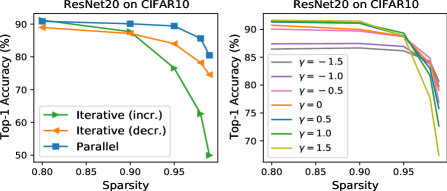
Figure 4: Left: Comparing parallel training with iterative training. Right: Ablation studies on the correction factor $\gamma$.

C.3 Cosine Similarity Analysis

In Fig. 1 Right of Sec. 3.2 in the main text, we choose two typical layers in ResNet20 and plot their cosine similarity between the loss gradients of different subnets along with training iterations. Here, we show the cosine similarity between the loss gradients of all layers in ResNet20, see in Fig. 5. Recall that we parallelly train 5 subnets of ResNet20 [11] with the overall sparsity $s_{1:5}=0.8,0.9,0.95,0.98,0.99$ on CIFAR10, and let the 5 loss items weighted equally, i.e. $\pi_{1:5}=0.2$. We plot the cosine similarity between the loss gradients of 5 subnets (i.e. $(\partial\mathcal{L}(\bm{w}_{k})/\partial\bm{w}_{k})\odot\bm{m}_{k}$ with $k=1,...,5$) and that of the lowest sparsity subnet (i.e. $(\partial\mathcal{L}(\bm{w}_{1})/\partial\bm{w}_{1})\odot\bm{m}_{1}$) along with the training iterations. It shows that the loss gradients of different subnets are always positively correlated with each other. The results also verify that multiple subnets are jointly trained towards the optimal point in the loss landscape.

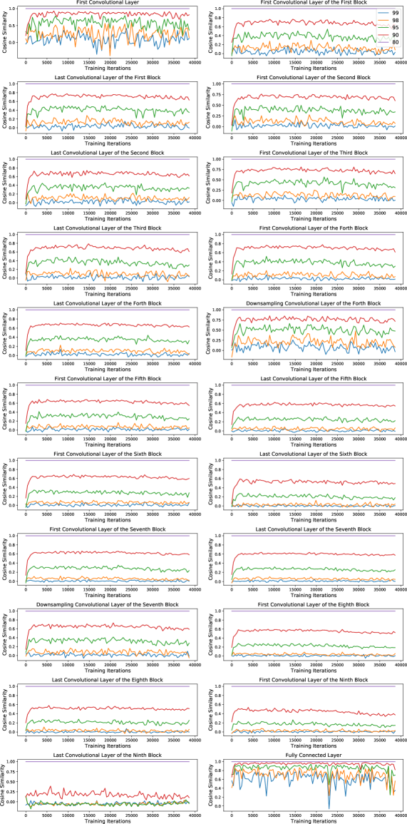
Figure 5: The cosine similarity between the loss gradients of 5 subnets (with sparsity $0.8,0.9,0.95,0.98,0.99$) and that of the lowest sparsity subnet (with sparsity 0.8) along with the parallel training iterations. We show all conv layers and the fc layer in ResNet20.

References

- [1] Google xnnpack - github repository, 2019. Accessed: 2021-10-20.
- [2] Arm vela compiler, 2020. Accessed: 2021-10-20.
- [3] Martín Abadi, Ashish Agarwal, Paul Barham, Eugene Brevdo, Zhifeng Chen, Craig Citro, Greg S. Corrado, Andy Davis, Jeffrey Dean, Matthieu Devin, Sanjay Ghemawat, Ian Goodfellow, Andrew Harp, Geoffrey Irving, Michael Isard, Yangqing Jia, Rafal Jozefowicz, Lukasz Kaiser, Manjunath Kudlur, Josh Levenberg, Dandelion Mané, Rajat Monga, Sherry Moore, Derek Murray, Chris Olah, Mike Schuster, Jonathon Shlens, Benoit Steiner, Ilya Sutskever, Kunal Talwar, Paul Tucker, Vincent Vanhoucke, Vijay Vasudevan, Fernanda Viégas, Oriol Vinyals, Pete Warden, Martin Wattenberg, Martin Wicke, Yuan Yu, and Xiaoqiang Zheng. TensorFlow: Large-scale machine learning on heterogeneous systems, 2015. Software available from tensorflow.org.
- [4] Han Cai, Chuang Gan, Tianzhe Wang, Zhekai Zhang, and Song Han. Once-for-all: Train one network and specialize it for efficient deployment. In International Conference on Learning Representations (ICLR), 2020.
- [5] Matthieu Courbariaux, Yoshua Bengio, and Jean-Pierre David. Binaryconnect: Training deep neural networks with binary weights during propagations. In Proceedings of Advances in Neural Information Processing Systems (NeurIPS), pages 3123–3131, 2015.
- [6] Erich Elsen, Marat Dukhan, Trevor Gale, and Karen Simonyan. Fast sparse convnets. In 2020 IEEE/CVF Conference on Computer Vision and Pattern Recognition (CVPR), 2020.
- [7] Utku Evci, Trevor Gale, Jacob Menick, Pablo Samuel Castro, and Erich Elsen. Rigging the lottery: Making all tickets winners. In Proceedings of the 38th International Conference on Machine Learning (ICML), 2021.
- [8] Jonathan Frankle and Michael Carbin. The lottery ticket hypothesis: Finding sparse, trainable neural networks. In International Conference on Learning Representations (ICLR), 2019.
- [9] Song Han, Huizi Mao, and William J Dally. Deep compression: Compressing deep neural networks with pruning, trained quantization and huffman coding. In Proceedings of International Conference on Learning Representations (ICLR), 2016.
- [10] Yizeng Han, Gao Huang, Shiji Song, Le Yang, Honghui Wang, and Yulin Wang. Dynamic neural networks: A survey. IEEE Transactions on Pattern Analysis and Machine Intelligence, page 1–1, 2021.
- [11] Kaiming He, Xiangyu Zhang, Shaoqing Ren, and Jian Sun. Deep residual learning for image recognition. In 2016 IEEE/CVF Conference on Computer Vision and Pattern Recognition (CVPR), 2016.
- [12] Mark Horowitz. 1.1 computing’s energy problem (and what we can do about it). In 2014 IEEE International Solid-State Circuits Conference Digest of Technical Papers (ISSCC), 2014.
- [13] Andrew Howard, Mark Sandler, Bo Chen, Weijun Wang, Liang-Chieh Chen, Mingxing Tan, Grace Chu, Vijay Vasudevan, Yukun Zhu, Ruoming Pang, Vijay Vasudevan, Quoc Le, and Hartwig Adam. Searching for mobilenetv3. In 2019 IEEE/CVF International Conference on Computer Vision (ICCV), Oct 2019.
- [14] Andrew G. Howard, Menglong Zhu, Bo Chen, Dmitry Kalenichenko, Weijun Wang, Tobias Weyand, Marco Andreetto, and Hartwig Adam. Mobilenets: Efficient convolutional neural networks for mobile vision applications. 2017.
- [15] Gao Huang, Danlu Chen, Tianhong Li, Felix Wu, Laurens van der Maaten, and Kilian Weinberger. Multi-scale dense networks for resource efficient image classification. In International Conference on Learning Representations (ICLR), 2018.
- [16] Itay Hubara, Brian Chmiel, Moshe Island, Ron Banner, Seffi Naor, and Daniel Soudry. Accelerated sparse neural training: A provable and efficient method to find n:m transposable masks. In Proceedings of Advances in Neural Information Processing Systems (NeurIPS), 2021.
- [17] Alex Krizhevsky, Vinod Nair, and Geoffrey Hinton. Cifar (canadian institute for advanced research), 2009.
- [18] Liangzhen Lai, Naveen Suda, and Vikas Chandra. Cmsis-nn: Efficient neural network kernels for arm cortex-m cpus. 2018.
- [19] Seulki Lee and Shahriar Nirjon. Subflow: A dynamic induced-subgraph strategy toward real-time dnn inference and training. In 2020 IEEE Real-Time and Embedded Technology and Applications Symposium (RTAS), pages 15–29, 2020.
- [20] Bailin Li, Bowen Wu, Jiang Su, Guangrun Wang, and Liang Lin. Eagleeye: Fast sub-net evaluation for efficient neural network pruning. In Proceedings of European Conference on Computer Vision (ECCV), 2020.
- [21] Changlin Li, Guangrun Wang, Bing Wang, Xiaodan Liang, Zhihui Li, and Xiaojun Chang. Dynamic slimmable network. In 2020 IEEE/CVF Conference on Computer Vision and Pattern Recognition (CVPR), 2020.
- [22] Zechun Liu, Haoyuan Mu, Xiangyu Zhang, Zichao Guo, Xin Yang, Tim Kwang-Ting Cheng, and Jian Sun. Metapruning: Meta learning for automatic neural network channel pruning. In 2019 IEEE/CVF International Conference on Computer Vision (ICCV), Oct 2019.
- [23] Asit Mishra, Jorge Albericio Latorre, Jeff Pool, Darko Stosic, Dusan Stosic, Ganesh Venkatesh, Chong Yu, and Paulius Micikevicius. Accelerating sparse deep neural networks. 2021.
- [24] Adam Paszke, Sam Gross, Soumith Chintala, Gregory Chanan, Edward Yang, Zachary DeVito, Zeming Lin, Alban Desmaison, Luca Antiga, and Adam Lerer. Automatic differentiation in pytorch. In Proceedings of NIPS Autodiff Workshop: The Future of Gradient-based Machine Learning Software and Techniques, 2017.
- [25] Alexandra Peste, Eugenia Iofinova, Adrian Vladu, and Dan Alistarh. Ac/dc: Alternating compressed/decompressed training of deep neural networks. In Proceedings of Advances in Neural Information Processing Systems (NeurIPS), 2021.
- [26] Pytorch. Pytorch example on resnet, 2019. Accessed: 2021-10-15.
- [27] Zhongnan Qu, Zimu Zhou, Yun Cheng, and Lothar Thiele. Adaptive loss-aware quantization for multi-bit networks. In 2020 IEEE/CVF Conference on Computer Vision and Pattern Recognition (CVPR), 2020.
- [28] Mohammad Rastegari, Vicente Ordonez, Joseph Redmon, and Ali Farhadi. Xnor-net: Imagenet classification using binary convolutional neural networks. In Proceedings of European Conference on Computer Vision (ECCV), pages 525–542, 2016.
- [29] Alex Renda, Jonathan Frankle, and Michael Carbin. Comparing fine-tuning and rewinding in neural network pruning. In International Conference on Learning Representations (ICLR), 2020.
- [30] Olga Russakovsky, Jia Deng, Hao Su, Jonathan Krause, Sanjeev Satheesh, Sean Ma, Zhiheng Huang, Andrej Karpathy, Aditya Khosla, Michael Bernstein, Alexander C. Berg, and Li Fei-Fei. Imagenet large scale visual recognition challenge. International Journal of Computer Vision, 115(3):211–252, 2015.
- [31] Mark Sandler, Andrew Howard, Menglong Zhu, Andrey Zhmoginov, and Liang-Chieh Chen. Mobilenetv2: Inverted residuals and linear bottlenecks. In 2018 IEEE/CVF Conference on Computer Vision and Pattern Recognition (CVPR), 2018.
- [32] Wei Sun, Aojun Zhou, Sander Stuijk, Rob G. J. Wijnhoven, Andrew Nelson, Hongsheng Li, and Henk Corporaal. Dominosearch: Find layer-wise fine-grained n:m sparse schemes from dense neural networks. In Proceedings of Advances in Neural Information Processing Systems (NeurIPS), 2021.
- [33] Mingxing Tan and Quoc V. Le. Efficientnet: Rethinking model scaling for convolutional neural networks. In Proceedings of the 36th International Conference on Machine Learning (ICML), 2019.
- [34] Thomas Verelst and Tinne Tuytelaars. Dynamic convolutions: Exploiting spatial sparsity for faster inference. In 2020 IEEE/CVF Conference on Computer Vision and Pattern Recognition (CVPR), 2020.
- [35] Jiahui Yu and Thomas Huang. Autoslim: Towards one-shot architecture search for channel numbers. 2019.
- [36] Jiahui Yu and Thomas Huang. Universally slimmable networks and improved training techniques. In 2019 IEEE International Conference on Computer Vision (ICCV), Oct 2019.
- [37] Jiahui Yu, Linjie Yang, Ning Xu, Jianchao Yang, and Thomas Huang. Slimmable neural networks. In International Conference on Learning Representations (ICLR), 2019.
- [38] Aojun Zhou, Yukun Ma, Junnan Zhu, Jianbo Liu, Zhijie Zhang, Kun Yuan, Wenxiu Sun, and Hongsheng Li. Learning n:m fine-grained structured sparse neural networks from scratch. In International Conference on Learning Representations (ICLR), 2021.