Stable Morse flow trees

Abstract

Let $L\subset J^{1}M$ be a closed Legendrian, in the 1-jet space of a closed manifold $M$, with simple front singularities. We define a natural generalization of a Morse flow tree, namely, a stable flow tree. We show a result analogous to Gromov compactness for stable maps – a sequence of stable flow trees, with a uniform edge bound, has a subsequence that Floer-Gromov converges to a stable flow tree. Moreover, we realize Floer-Gromov convergence as the topological convergence of a certain moduli space of stable flow trees.

1.  Introduction

Let $(M,g)$ be a closed Riemannian $n$-manifold, let $J^{0}M\coloneqq M\times\mathbb{R}$ be $M$’s 0-jet space, and let $J^{1}M\coloneqq T^{*}M\times\mathbb{R}$ be $M$’s 1-jet space. We endow $J^{1}M$ with the standard contact structure $\xi$, given as the kernel of $dz-\alpha$, where $z$ is the $\mathbb{R}$-coordinate and $\alpha$ is the tautological 1-form on $T^{*}M$. An $n$-dimensional submanifold $L\subset J^{1}M$ is called Legendrian if it is an integral submanifold of $\xi$. We also endow $T^{*}M$ with the standard symplectic structure, given as $-d\alpha$. An $n$-dimensional submanifold of $T^{*}M$ is called Lagrangian if $-d\alpha$ identically vanishes on it.

(Morse) Flow trees were introduced in [Ekh07] to help compute the contact homology of Legendrians in 1-jet spaces. Specifically, Legendrian contact homology is an isotopy invariant of Legendrians in the framework of Symplectic Field Theory (see [EGH00]). The rigorous construction of Legendrian contact homology in 1-jet spaces was done in [EES07], where the construction involves counting rigid pseudo-holomorphic disks with punctures asymptotic to Reeb chords on the Legendrian. Finding pseudo-holomorphic disks involves solving a non-linear first order partial differential equation, thus explicit computations are quite difficult. The main result of [Ekh07] reduces this infinite-dimensional problem to a finite-dimensional problem in Morse theory by building a 1-1 correspondence between (certain types of) flow trees and (certain types of) pseudo-holomorphic disks (after appropriate perturbations of the involved data). The relation between Morse theory and pseudo-holomorphic disks can be found in the Floer-theoretic case (see [Flo89] and [FO97]), and the power of flow trees can be seen in the computations of Legendrian contact homology in [EENS13], [EN18], [RG19], and [Riz11].

A flow tree is essentially a combinatorial tree, where each edge is assigned a gradient flow of some difference of functions locally defined on $M$, where $L$ is locally the multi 1-jet graph of these local functions. In this article, we generalize flow trees by constructing stable flow trees (see Definition 4.5), in analogy to the generalization of pseudo-holomorphic curves to stable maps. Recall that Gromov compactness says: for a sequence of stable maps, with uniformly bounded energy, there exists a Gromov convergent subsequence. We define a notion of convergence of stable flow trees, called Floer-Gromov convergence (see Definition 4.9). The number of edges of a stable flow tree then plays the role of the energy of a pseudo-holomorphic disk, namely, we prove the following result:

Theorem 1.1.

Let $T_{\nu}$ be a sequence of stable flow trees. If $\sup_{\nu}\left\lvert\mathcal{E}_{\nu}\right\rvert<\infty$, where $\left\lvert\mathcal{E}_{\nu}\right\rvert$ is the number of edges of $T_{\nu}$, then $T_{\nu}$ has a Floer-Gromov convergent subsequence.

Given Ekholm’s 1-1 correspondence between flow trees and pseudo-holomorphic disks, such a result is expected. We define the moduli space

$$\overline{\mathcal{L}}(L,N)\coloneqq\left\{T\in\mathcal{L}(L):\begin{aligned} &\textrm{there exists a sequence $T_{\nu}\in\mathcal{L}(L,N)$}\\ &\textrm{that Floer-Gromov converges to $T$}\end{aligned}\right\},$$

where $\mathcal{L}(L)$ is the set of stable flow trees and $\mathcal{L}(L,N)$ is the set of stable flow trees, with at most $N$ edges. The definition of Floer-Gromov convergence is a natural one to consider, due to the following result:

Theorem 1.2.

There exists a unique topology on the set $\overline{\mathcal{L}}(L,N)$ such that the topological convergence is equivalent to Floer-Gromov convergence. Moreover, $\overline{\mathcal{L}}(L,N)$ is compact with respect to this topology.

This article is structured as follows. In Section 2, we recall the theory of flow trees following [Ekh07]. In Section 3, we (formally) compactify the various moduli spaces of gradient flows of local function differences. This is necessary because Floer-Gromov convergence will essentially reduce to the convergence of the various sequences of edges. In Section 4, we define stable flow trees, Floer-Gromov convergence, and prove Theorems 1.1 and 1.2. Finally, in Section 5, we exhibit an example of Floer-Gromov convergence, following an example in Section 7 of [Ekh07].

Acknowledgements

The author would like to Christopher Woodward for suggesting this project, and Soham Chanda, Tyler Lane, Eric Kilgore, and Benoit Pausader for conversations. The author was partially supported by the 2021 DIMACS REU, the Rutgers Department of Mathematics, and NSF grant DMS-1711070 while completing the work for this project.

2.  Preliminaries

2.1.  Local functions and local gradients

As before, let $(M,g)$ be a closed Riemannian $n$-manifold and let $L\subset J^{1}M$ be a closed Legendrian submanifold. We will assume that $L$ is chord generic, i.e., that $L$ has finitely many isolated Reeb chords. This condition may be achieved after generic perturbation and is stable.

Consider the Lagrangian projection $\Pi_{\mathbb{C}}:J^{1}M\to T^{*}M$, then $\Pi_{\mathbb{C}}(L)$ is an immersed Lagrangian. Since the Reeb field of the standard contact structure $\xi$ on $J^{1}M$ is $\partial_{z}$, it follows that there is a 1-1 correspondence between Reeb chords on $L$ and self-transverse double points of $\Pi_{\mathbb{C}}(L)$.

We will assume that $L$ has simple front singularities, which means $L$ satisfies the following conditions.

• The base projection $\Pi:J^{1}M\to M$, restricted to $L$, is an immersion outside of a closed codimension 1 submanifold $\Sigma\subset L$.

• For any $\tilde{p}\in\Sigma$, the front projection $\Pi_{F}:J^{1}M\to J^{0}M$, restricted to $L$, has a standard cusp-edge singularity at $\tilde{p}$. Precisely, there exists coordinates $y=(y_{1},\ldots,y_{n})$ around $\tilde{p}\in L$ and there exists coordinates $x=(x_{1},\ldots,x_{n})$ around $\Pi(\tilde{p})\in M$, such that the following holds. If $z$ is the $\mathbb{R}$-coordinate on $J^{0}(M)$, then $\Pi_{F}(y)=(x(y),z(y))$, where

  $$x_{1}(y) =\dfrac{1}{2}y_{1}^{2},$$

  $$x_{i}(y) =y_{i},\;\;i\geq 2,$$

  $$z(y) =\dfrac{1}{3}y_{1}^{3}+b\dfrac{1}{2}y_{1}^{2}+a_{2}y_{2}+\dots+a_{n}y_{n},\;\;a_{j},b\in\mathbb{R}.$$

• The base projection, restricted to $\Sigma$, is a self-transverse immersion.

In dimensions greater than 1, this condition is not generic. We refer to $\Pi(\Sigma)\subset M$ as the singular set. We will assume that $\Pi|_{\Sigma}$ is self-transverse in the following way: we assume there is a stratification

$$\Pi(\Sigma)\eqqcolon\Sigma_{1}\supset\cdots\supset\Sigma_{k},$$

where $\Sigma_{i}$ is the set of self-intersection points of $\Pi|_{\Sigma}$ of multiplicity at least $i$, such that $\Sigma_{i}$ has codimension $i$ in $M$ (hence $i\leq n$). This condition may be achieved after generic perturbation and is stable.

Locally, $L$ is the multi 1-jet graph of local functions defined on the base $M$, as follows.

If $p\in M\setminus\Pi(\Sigma)$, then there exists an open neighborhood $U\subset M\setminus\Pi(\Sigma)$ of $p$, and there exists $k$ disjoint open sets $U_{1},\ldots,U_{k}\subset L\setminus\Sigma$, such that

$$U_{i}=\{(x,d(f_{i})_{x},f_{i}(x)):x\in U\},$$

for some functions $f_{i}\in C^{\infty}(U)$, and such that each $U_{i}$ is diffeomorphic to $U$ via the base projection. Each $U_{i}$ is called a smooth sheet lying over $p$.

Similarly, a point $p\in\Sigma_{j}\setminus\Sigma_{j+1}$ may have smooth sheets lying over it. In addition, there exists an open neighborhood $V\subset\Sigma_{j}$ of $p$, and there exists $j$ disjoint open sets $V_{1},\ldots,V_{j}\subset\Sigma$, such that each $V_{i}$ is diffeomorphic to $V$ via the base projection. If we consider a sufficiently small neighborhood $U\subset M$ of $p$, then each $\Pi(V_{i})$ subdivides $U$ into two components $\{U_{i}^{\pm}\}$. Moreover, there exists two functions $\{f_{i}^{1},f_{i}^{2}\}$ defined on $U_{i}^{+}$ such that both functions: extend to $\overline{U}_{i}^{+}$, agree on $\partial U_{i}^{+}$, and have differentials whose limits agree on $\partial U_{i}^{+}$ when approached from $U_{i}^{+}$. Since $L$ has simple front singularities, the local functions $\{f_{i}^{1},f_{i}^{2}\}$ are of the form

$$f^{1}_{i}(x) =\dfrac{1}{3}(2x_{1})^{3/2}+bx_{1}+a_{2}x_{2}+\dots+a_{n}x_{n},$$

$$f^{2}_{i}(x) =-\dfrac{1}{3}(2x_{1})^{3/2}+bx_{1}+a_{2}x_{2}+\dots+a_{n}x_{n},$$ (1)

where $\{x_{1}>0\}$, and the common limits of the differentials on $\{x_{1}=0\}$ is

$$bdx_{1}+a_{2}dx_{2}+\cdots+a_{n}dx_{n},$$

where we use the coordinates associated to the standard cusp-edge singularity $\tilde{p}_{i}$ defined by $\{\tilde{p}_{i}\}\coloneqq\Pi^{-1}(p)\cap V_{i}$.

Remark 2.1.

By compactness of $M$ and $L$, there are only finitely many local functions under consideration.

Let $f_{i},f_{j}$ be local functions whose domains overlap on, some open set $U\subset M$, and consider their local function difference $F_{ij}\coloneqq f_{i}-f_{j}\in C^{\infty}(U)$. We call a curve $\phi:I\to M$, where $I\subset\mathbb{R}$ is an interval, a gradient flow of $L$ if $\phi$ is a solution to the gradient flow equation

$$\dot{\phi}=-\nabla F_{ij}(\phi),$$

for some local function difference $F_{ij}$. A 1-jet lift of $\phi$ is an unordered pair

$$\left\{\tilde{\phi}^{1},\tilde{\phi}^{2}\right\}$$

of continuous lifts $\tilde{\phi}^{k}:I\to L$ of $\phi$, such that either: $\tilde{\phi}^{1}$ lies in the sheet determined by $f_{i}$ and $\tilde{\phi}^{2}$ lies in the sheet determined by $f_{j}$, or vice versa; and satisfies

$$\tilde{\phi}^{1}(t_{0})=\tilde{\phi}^{2}(s_{0})$$

if and only if $t_{0}=s_{0}$ and the point $\tilde{\phi}^{1}(t_{0})$ lies in $\Sigma$ over $\phi(t_{0})$ (equivalently, $\tilde{\phi}^{2}(s_{0})$ lies in $\Sigma$ over $\phi(s_{0})$). In other words, the 1-jet lifts may only meet in $\Sigma$. We also define a cotangent lift of $\phi$ as an unordered pair

$$\left\{\overline{\phi}^{1}\coloneqq\Pi_{\mathbb{C}}\circ\tilde{\phi}^{1},\overline{\phi}^{2}\coloneqq\Pi_{\mathbb{C}}\circ\tilde{\phi}^{2}\right\}.$$

Definition 2.2 (Definition 2.9 in [Ekh07]).

The flow orientation of $\tilde{\phi}^{1}$ at $\tilde{p}\in L$ is given by the unique lift of the vector

$$-\nabla F_{ij}(\Pi(\tilde{p}))\in T_{\Pi(\tilde{p})}M$$

to $T_{\tilde{p}}L$, where $f_{i}$ is the local function determined by $\tilde{\phi}^{1}$. We similarly orient $\tilde{\phi}^{2}$.

Remark 2.3.

Definition 2.2 gives a natural orientation of a cotangent lift.

By existence and uniqueness theorems of ODEs, we see that any gradient flow of $L$ has a maximal interval of definition. Any gradient flow of $L$ defined on its maximal interval of definition will be called a maximally extended gradient flow of $L$. The asymptotic behavior of maximally extended gradient flows is given by the following lemma:

Lemma 2.4 (Lemma 2.8 in [Ekh07]).

Let $\Phi:I\to M$ be a maximally extended gradient flow of $L$ associated to $F_{ij}$. If $I$ is an interval with an infinite end, i.e., $I$ equals $(a,\infty)$ or $(-\infty,b)$ for $a,b\in\mathbb{R}\cup\{\infty\}$, then

$$\lim_{t\to\pm\infty}\Phi(t)\in\operatorname{Crit}(F_{ij}),$$

where $\operatorname{Crit}(F_{ij})$ is the set of critical points of $F_{ij}$. If $I$ is an interval with a compact end, i.e., $I$ equals $(a,\ell]$ or $[\ell,b)$ for $a,b\in\mathbb{R}\cup\{\infty\}$ and $\ell\in\mathbb{R}$, then

$$\lim_{t\to\ell}\tilde{\Phi}^{k}(t)\in\Sigma,\;\;\textrm{$k=1$ or $k=2$}$$

for some 1-jet lift of $\Phi$. In particular, $\Phi(\ell)$ lies in $\Pi(\Sigma)\cap\overline{U}$.

Proof.

See Lemma 2.8 in [Ekh07]. ∎

The asymptotic behavior of (maximally extended) gradient flows of $L$ allows us to characterize them.

Definition 2.5.

Let $\phi$ be a gradient flow of $L$ associated to $F_{ij}$ with maximal extension $\Phi$. Then $\phi$ (respectively $\Phi$) is called a:

• (maximally extended) Morse flow if $\Phi$ connects two points of $\operatorname{Crit}(F_{ij})$,

• (maximally extended) fold emanating flow if $\Phi$ connects a point of $\Pi(\Sigma)\cap\overline{U}$ to a point of $\operatorname{Crit}(F_{ij})$,

• (maximally extended) fold terminating flow if $\Phi$ connects a point of $\operatorname{Crit}(F_{ij})$ to a point of $\Pi(\Sigma)\cap\overline{U}$,

• (maximally extended) singular flow if $\Phi$ connects two points of $\Pi(\Sigma)\cap\overline{U}$.

2.2.  Flow trees

Let $T$ be a tree with edge set $\mathcal{E}$ and vertex set $\mathcal{V}$. A source tree is a finite-edge tree $T$ (where the edge set may be empty) such that, at each $k$-valent vertex $v$, $k\geq 3$, the edges adjacent to $v$ are cyclically labelled.

Definition 2.6 (Definition 2.10 in [Ekh07]).

A true flow tree of $L$ is a continuous map $\phi:T\to M$, where $T$ is a source tree, that satisfies the following conditions.

• If $e$ is an edge of $T$, then $\phi:e\to M$ is an injective parameterization of a gradient flow of $L$. In particular, $\phi:e\to M$ cannot be constant.

• Let $v$ be a $k$-valent vertex of $T$ with (cyclically ordered) edges $e_{v,1},\ldots,e_{v,k}$. We require that there exists cotangent lifts

  $$\left\{\overline{\phi}^{1}_{v,j},\overline{\phi}^{2}_{v,j}\right\},$$

  for each edge $e_{v,j}$, such that

  $$\overline{p}_{v,j}\coloneqq\overline{\phi}^{2}_{v,j}(v)=\overline{\phi}^{1}_{v,j+1}(v)\in\Pi_{\mathbb{C}}(L)$$

  and such that the flow orientation of $\overline{\phi}^{2}_{v,j}$ at $\overline{p}_{v,j}$ is directed toward $\overline{p}_{v,j}$ if and only if the flow orientation of $\overline{\phi}^{1}_{v,j+1}$ at $\overline{p}_{v,j}$ is directed away from $\overline{p}_{v,j}$.

• We require that the aforementioned cotangent lifts of all the edges yield an oriented loop in $\Pi_{\mathbb{C}}(L)$.

Definition 2.7.

Let $T$ be a true flow tree. A removable vertex of $T$ is a 2-valent vertex $v$ such that: the assigned gradient flows of the adjacent edges, $\phi_{v,1}$ and $\phi_{v,2}$, are both gradient flows of the same local function difference $F_{ij}$, and these gradient flows concatenate together at

$$p_{v}\coloneqq\phi_{v,1}(v)=\phi_{v,2}(v)$$

to give a single gradient flow $\phi_{v}$ of $F_{ij}$.

The name removable vertex is warranted because these vertices are erroneous in the following sense. Given any true flow tree, we may arbitrarily add a removable vertex by picking an edge and adding a 2-valent vertex somewhere along that edge.

Remark 2.8.

Definition 2.6 is the original definition of a flow tree given in [Ekh07]. However, this definition is problematic because it allows the phenomenon of removable vertices. The reason these kinds of vertices are problematic is because the dimension formulas for flow trees (Definitions 3.4 and 3.5 in [Ekh07]) do not hold for trees with removable vertices. This motivates the following definition.

Definition 2.9.

A (parameterized) flow tree is a true flow tree that does not have any removable vertices.

Lastly, we will assume that $L$ satisfies the preliminary transversality condition, found in pages 1101-1103 in [Ekh07]. We will not define this condition since its definition is quite long-winded. In short, the preliminary transversality condition affects how the various sheets of the Legendrian are allowed to meet, and the consequences of the condition ensure gradient flows of $L$ meet the singular set in a locally stable fashion. In particular, any gradient flow of $L$ may only meet the singular set with order of contact at most $n$ (hence no gradient flow of $L$ may flow along the singular set). This condition may be achieved after generic perturbation and is stable.

3.  Compactification of edges

3.1.  Morse theory

Let $F_{ij}$ be a local function difference defined on some open set $U\subset M$. Since the Reeb chords of $L$ are in 1-1 correspondence with the self-transverse double points of $\Pi_{\mathbb{C}}(L)$, and $L$ is chord generic by assumption, it follows that $F_{ij}$ is a Morse function with finitely many critical points. Moreover, we will assume that no critical point of any local function difference lies in the singular set. This condition may be achieved by generic perturbation and is stable.

Floer-Gromov convergence of stable flow trees will essentially reduce to convergence of the various sequences of edges. Therefore, we must first compactify the various moduli spaces of gradient flows associated to our local function differences. Since each local function difference is Morse, we will use the techniques of standard Morse theory, following Section 2 of [AD14]. However, we will only formally compactify the moduli spaces in this section, i.e., we will not build topologies on the moduli spaces of gradient flows such that the desired sequences topologically converge – we will only formally define the notion of edge convergence (Definition 3.10).

Also, we will make the following (non-generic) assumption: the Riemannian metric $g$ on $M$ is Euclidean in Morse neighborhoods of critical points of local function differences. This assumption is usually made in the literature to simplify various technical arguments regarding the interactions of unstable manifolds, stable manifolds, and Morse neighborhoods. We will recall the relevant definitions now.

Recall that the Morse lemma states:

Lemma 3.1.

Suppose $c\in\operatorname{Crit}(F_{ij})$, then there exists a neighborhood $\Omega(c)\subset U$ and a diffeomorphism $\varphi:\Omega(c)\to\varphi\left(\Omega(c)\right)\subset\mathbb{R}^{n}$ such that

$$\left(F_{ij}\circ\varphi^{-1}\right)(x_{1},\ldots,x_{n})=F_{ij}(c)-\sum_{k=1}^{m}x_{k}^{n}+\sum_{k=m+1}^{n}x_{k}^{2}.$$

The number $I(c)\coloneqq m$ appearing in the Morse lemma is called the Morse index of $c$ and the neighborhood $\Omega(c)$ appearing in the Morse lemma is called a Morse neighborhood of $c$.

In the rest of this section, we will use the fact that our unstable manifolds, stable manifolds, and Morse neighborhoods are of a particular form by our (non-generic) assumption on $g$, which we now describe. See Pages 24-29 of [AD14] for details. Let $c\in\operatorname{Crit}(F_{ij})$ and let $V\coloneqq\varphi\left(\Omega(c)\right)\subset\mathbb{R}^{n}$ be the image of a Morse neighborhood of $c$, where we assume $\varphi$ identifies $c$ with the origin. If we denote by $Q$ the quadratic form $d^{2}\left(F_{ij}\circ\varphi^{-1}\right)_{0}$, i.e., the Hessian of $f$ at the origin, then we see $Q$ is: negative-definite on a subspace $V_{-}\subset\mathbb{R}^{n}$ of dimension $I(c)$ and positive-definite on a complimentary subspace $V_{+}\subset\mathbb{R}^{n}$. Let $\epsilon,\eta>0$ be sufficiently small real numbers. It follows that $V$ is of the form

$$V=\left\{x\in\mathbb{R}^{n}:\begin{aligned} &-\epsilon<Q(x)<\epsilon\\ &\left\lvert x_{-}\right\rvert^{2}\left\lvert x_{+}\right\rvert^{2}\leq\eta(\epsilon+\eta)\end{aligned}\right\},$$

where $x=x_{-}\oplus x_{+}$ for $x_{\pm}\in V_{\pm}$. The boundary of $V$ consists of three parts:

$$\partial_{\pm}V \coloneqq\{x\in V:Q(x)=\pm\epsilon,\;\;\left\lvert x_{\mp}\right\rvert^{2}\leq\eta\},$$

$$\partial_{0}V \coloneqq\{x\in V:\left\lvert x_{-}\right\rvert^{2}\left\lvert x_{+}\right\rvert^{2}=\eta(\epsilon+\eta)\}.$$

See Figure 1.

Figure 1: The image $V$ of the Morse neighborhood $\Omega(c)$. The black border is $\partial V$. The blue lines are the level sets of $F_{ij}$. The red lines are gradient flows of $F_{ij}$. The axes are the sets $V_{\pm}$. The sets $\partial_{\pm}V$ are contained in the level sets that intersect $V_{\pm}$.

The unstable manifold and stable manifold of $c$ are defined as:

$$W^{u}(c) \coloneqq\{x\in M:\textrm{$\exists\phi$ a gradient flow at $x$ with $\lim_{t\to-\infty}\phi(t)=c$}\},$$

$$W^{s}(c) \coloneqq\{x\in M:\textrm{$\exists\phi$ a gradient flow at $x$ with $\lim_{t\to\infty}\phi(t)=c$}\},$$

respectively. We note that, by the above description of $\Omega(c)$,

$$V_{-} =W^{u}(c)\cap\Omega(c),$$

$$V_{+} =W^{s}(c)\cap\Omega(c).$$

Moreover, by the above description of $\Omega(c)$, we see that

$$W^{u}(c)\cap\Omega(c) \cong S^{I(c)-1},$$

$$W^{s}(c)\cap\Omega(c) \cong S^{n-I(c)-1}.$$

We will require the following two lemmas later in this section.

Lemma 3.2 (Lemma 3.2.5 in [AD14]).

Let $x\in U\setminus\operatorname{Crit}(F_{ij})$ and let $x_{\nu}\in U$ be a sequence converging to $x$. Suppose $y_{\nu}$ and $y$ are points lying on the same gradient flows of $F_{ij}$ as $x_{\nu}$ and $x$, respectively, and suppose that $F_{ij}(y_{\nu})=F_{ij}(y)$, then the sequence $y_{\nu}$ converges to $y$.

Proof.

See Lemma 3.2.5 in [AD14]. ∎

Before the second lemma, we have to define some terminology. Recall the local form (2.1) for local functions near the cusp-edge. It follows that the gradient $\nabla F_{ij}$ is non-singular on $\overline{U}$. Suppose $x\in\Pi(\Sigma)$ and $\phi$ is a gradient flow of $F_{ij}$ that passes through $x$, then, since the gradient $\nabla F_{ij}$ is non-singular at $x$, there exists an embedded neighborhood $V\subset\Pi(\Sigma)$ of $x$ and a coordinate chart $\varphi:W\subset M\to\mathbb{R}^{n}$, centered at $x$, that satisfies the following conditions:

• $\varphi$ maps $x$ to the origin,

• $\varphi(V)$ divides $\mathbb{R}^{n}$ into two components, $W^{-}\coloneqq\varphi(W\cap U)$ and $W^{+}\coloneqq\varphi(W\cap U^{c})$,

• $-\nabla F_{ij}|_{W\cap U}$ corresponds to the coordinate vector field $\partial_{x_{1}}|_{W^{-}}$,

• and $\phi$ corresponds to the unique flow line of $\partial_{x_{1}}|_{W^{-}\cap\{x_{2}=\cdots=x_{n}=0\}}$.

By the preliminary transversality condition, $-\nabla F_{ij}$ has order of contact at most $n$ with $\Pi(\Sigma)$, i.e., $\phi$ has order of contact at most $n$ with $\varphi(V)$ at the origin. In particular, $\phi$ cannot flow along $\varphi(V)$. Thus, there are two possibilities, $\phi$ either: can be extended (using the flow of $\partial_{x_{1}}$) to a flow line that touches $\varphi(V)$ at the origin and flows into $W^{+}$, or touches $\varphi(V)$ at the origin and remains in $W^{-}$. In simpler terms, $\phi$ either crosses $\Pi(\Sigma)$ or doesn’t. We say that $\phi$ ends on $\Pi(\Sigma)$ at $x$ if $\phi$ can be extended, in some coordinate chart as above, to a flow line that crosses $\Pi(\Sigma)$.

Lemma 3.3.

Let $\lambda$ be a gradient flow of $F_{ij}$ that ends on $\Pi(\Sigma)$ at $x$ and let $\phi_{\nu}$ be a sequence of gradient flows of $F_{ij}$. Suppose there exists a sequence of points $x_{\nu}$ in $\phi_{\nu}$ that converge to $x$, then there exists a subsequence of $\phi_{\nu}$ that ends on $\Pi(\Sigma)$ at $y_{\nu}$, such that the sequence $y_{\nu}$ converges to $x$.

Proof.

We construct a neighborhood $V\subset\Sigma$ of $x$ and a coordinate chart $\varphi:W\subset M\to\mathbb{R}^{n}$, centered at $x$, as above. For $\nu\gg 0$, we may assume that $\phi_{\nu}$ is identified with a flow line of $\partial_{x_{1}}|_{W^{-}}$, and we may assume that the sequence of points $x_{\nu}$ converges to the origin. Since $\lambda$ ends on $\Pi(\Sigma)$ at $x$, we may extend $\lambda$ to a flow line that crosses $\Pi(\Sigma)$. If we choose $z\in W^{+}$ on this extended flow line, then, by dependence of solutions to ODEs on initial conditions, there exists a sequence $z_{\nu}$ of points on (the extension, using the flow of $\partial_{x_{1}}$, of) $\phi_{\nu}$ that converge to $z$. By continuity, it follows that (the extension, using the flow of $\partial_{x_{1}}$, of) $\phi_{\nu}$ must cross $\Pi(\Sigma)$, for $\nu\gg 0$. In particular, $\phi_{\nu}$ ends on $\Pi(\Sigma)$ at some point $y_{\nu}$, and by passing to a subsequence, we see that the sequence $y_{\nu}$ converges to $x$, by dependence of solutions to ODEs on initial conditions. ∎

3.2.  Notation

In this section, we simply define notation and terminology.

Let $a,b\in\operatorname{Crit}(F_{ij})$, where $a$ and $b$ are not necessarily distinct. We define the following sets:

• $\mathcal{M}_{0}(F_{ij},a,b)$ the set of parameterized Morse flows of $F_{ij}$ connecting $a$ to $b$,

• $\mathcal{M}_{0}(F_{ij},\Pi(\Sigma),b)$ the set of parameterized fold emanating flows of $F_{ij}$ ending at $b$,

• $\mathcal{M}_{0}(F_{ij},a,\Pi(\Sigma))$ the set of parameterized fold terminating flows of $F_{ij}$ starting at $a$,

• and $\mathcal{M}_{0}(F_{ij},\Pi(\Sigma))$ the set of parameterized singular flows of $F_{ij}$.

We will drop the subscript in the notation if we would like to consider the set of maximally extended parameterized gradient flows of a certain type. There is a natural $\mathbb{R}$-action on each set of parameterized gradient flows, given by time-shift, i.e.,

$$(r,\phi)\mapsto\phi(t+r),\;\;r\in\mathbb{R}.$$

Thus, we may define the quotients:

• $\mathcal{L}_{0}(F_{ij},a,b)\coloneqq\mathcal{M}_{0}(F_{ij},a,b)/\mathbb{R}$ the set of (unparameterized) Morse flows of $F_{ij}$ connecting $a$ to $b$,

• $\mathcal{L}_{0}(F_{ij},\Pi(\Sigma),b)\coloneqq\mathcal{M}_{0}(F_{ij},\Pi(\Sigma),b)/\mathbb{R}$ the set of (unparameterized) fold emanating flows of $F_{ij}$ ending at $b$,

• $\mathcal{L}_{0}(F_{ij},a,\Pi(\Sigma))\coloneqq\mathcal{M}_{0}(F_{ij},a,\Pi(\Sigma))/\mathbb{R}$ the set of (unparameterized) fold terminating flows of $F_{ij}$ starting at $a$,

• and $\mathcal{L}_{0}(F_{ij},\Pi(\Sigma))\coloneqq\mathcal{M}_{0}(F_{ij},\Pi(\Sigma))/\mathbb{R}$ the set of (unparameterized) singular flows of $F_{ij}$.

Again, we will drop the subscript in the notation if we would like to only consider the set of maximally extended (unparameterized) gradient flows of a certain type.

Definition 3.4.

Let $c_{0},\ldots,c_{q+1}\in\operatorname{Crit}(F_{ij})$ such that

$$c_{0}=a,\;\;c_{q+1}=b.$$

A $q$-times broken Morse flow of $F_{ij}$ connecting $a$ to $b$, denoted $\lambda=(\lambda^{1},\ldots,\lambda^{q+1})$, is a concatenation of gradient flows:

$$\lambda^{1}\in\mathcal{L}_{0}(F_{ij},c_{0},c_{1}),\;\;\lambda^{k}\in\mathcal{L}(F_{ij},c_{k-1},c_{k}),\;\;\lambda^{q+1}\in\mathcal{L}_{0}(F_{ij},c_{q},c_{q+1}),$$

where $2\leq k\leq q$. We denote by $\mathcal{L}_{q,0}(F_{ij},a,b)$ the set of $q$-times broken Morse flows of $F_{ij}$ connecting $a$ to $b$.

Definition 3.5.

Let $c_{1},\ldots,c_{q+1}\in\operatorname{Crit}(F_{ij})$ such that

$$c_{q+1}=b.$$

A $q$-times broken fold emanating flow of $F_{ij}$ ending at $b$, denoted $\lambda=(\lambda^{1},\ldots,\lambda^{q+1})$, is a concatenation of gradient flows:

$$\lambda^{1}\in\mathcal{L}_{0}(F_{ij},\Pi(\Sigma),c_{1}),\;\;\lambda^{k}\in\mathcal{L}(F_{ij},c_{k-1},c_{k}),\;\;\lambda^{q+1}\in\mathcal{L}_{0}(F_{ij},c_{q},c_{q+1}),$$

where $2\leq k\leq q$. We denote by $\mathcal{L}_{q,0}(F_{ij},\Pi(\Sigma),b)$ the set of $q$-times broken fold emanating flows of $F_{ij}$ ending at $b$.

Definition 3.6.

Let $c_{0},\ldots,c_{q}\in\operatorname{Crit}(F_{ij})$ such that

$$c_{0}=a.$$

A $q$-times broken fold terminating flow of $F_{ij}$ starting at $a$, denoted $\lambda=(\lambda^{1},\ldots,\lambda^{q+1})$, is a concatenation of gradient flows:

$$\lambda^{1}\in\mathcal{L}_{0}(F_{ij},c_{0},c_{1}),\;\;\lambda^{k}\in\mathcal{L}(F_{ij},c_{k-1},c_{k}),\;\;\lambda^{q+1}\in\mathcal{L}_{0}(F_{ij},c_{q},\Pi(\Sigma)),$$

where $2\leq k\leq q$. We denote by $\mathcal{L}_{q,0}(F_{ij},a,\Pi(\Sigma))$ the set of $q$-times broken fold terminating flows of $F_{ij}$ starting at $a$.

Definition 3.7.

Let $c_{1},\ldots,c_{q}\in\operatorname{Crit}(F_{ij})$. For $q\geq 1$, a $q$-times broken singular flow of $F_{ij}$, denoted $\lambda=(\lambda^{1},\ldots,\lambda^{q+1})$, is a concatenation of gradient flows:

$$\lambda^{1}\in\mathcal{L}_{0}(F_{ij},\Pi(\Sigma),c_{1}),\;\;\lambda^{k}\in\mathcal{L}(F_{ij},c_{k-1},c_{k}),\;\;\lambda^{q+1}\in\mathcal{L}_{0}(F_{ij},c_{q},\Pi(\Sigma)),$$

where $2\leq k\leq q$. A $0$-times broken singular flow of $F_{ij}$ is simply a singular flow of $F_{ij}$. We denote by $\mathcal{L}_{q,0}(F_{ij},\Pi(\Sigma))$ the set of $q$-times broken singular flows $F_{ij}$.

Analogously, we may define a maximally extended $q$-times broken gradient flow of $F_{ij}$, of the appropriate type, by restricting to the case that the first and last component of the broken gradient flow are maximally extended gradient flows of $F_{ij}$, of the appropriate type. We may define the stratified sets:

$$\overline{\mathcal{L}}_{0}(F_{ij},a,b) \coloneqq\bigcup_{q\geq 0}\mathcal{L}_{q,0}(F_{ij},a,b),$$

$$\overline{\mathcal{L}}_{0}(F_{ij},\Pi(\Sigma),b) \coloneqq\bigcup_{q\geq 0}\mathcal{L}_{q,0}(F_{ij},\Pi(\Sigma),b),$$

$$\overline{\mathcal{L}}_{0}(F_{ij},a,\Pi(\Sigma)) \coloneqq\bigcup_{q\geq 0}\mathcal{L}_{q,0}(F_{ij},a,\Pi(\Sigma)),$$

$$\overline{\mathcal{L}}_{0}(F_{ij},\Pi(\Sigma)) \coloneqq\bigcup_{q\geq 0}\mathcal{L}_{q,0}(F_{ij},\Pi(\Sigma)).$$

Remark 3.8.

The above stratifications are finite because, there are only finitely many critical points of $F_{ij}$, and the value of $F_{ij}$ strictly decreases along any gradient flow.

We may define analogous stratified sets given by dropping the subscript. Finally, we will define the set of broken gradient flows of $F_{ij}$ as

$$\overline{\mathcal{L}}_{0}(F_{ij})\coloneqq\bigcup_{a,b\in\operatorname{Crit}(F_{ij})}\left\{\overline{\mathcal{L}}_{0}(F_{ij},a,b)\cup\overline{\mathcal{L}}_{0}(F_{ij},\Pi(\Sigma),b)\cup\overline{\mathcal{L}}_{0}(F_{ij},a,\Pi(\Sigma))\right\}\cup\overline{\mathcal{L}}_{0}(F_{ij},\Pi(\Sigma)),$$

where, again, omission of the subscript will be the analogous space where we consider only maximally extended broken gradient flows of $F_{ij}$. There is a natural inclusion $\mathcal{L}_{0}(F_{ij})\to\overline{\mathcal{L}}_{0}(F_{ij})$, where $\mathcal{L}_{0}(F_{ij})$ is the set of (unparameterized) gradient flows of $F_{ij}$:

$$\mathcal{L}_{0}(F_{ij})\coloneqq\bigcup_{a,b\in\operatorname{Crit}(F_{ij})}\left\{\mathcal{L}_{0}(F_{ij},a,b)\cup\mathcal{L}_{0}(F_{ij},\Pi(\Sigma),b)\cup\mathcal{L}_{0}(F_{ij},a,\Pi(\Sigma))\right\}\cup\mathcal{L}_{0}(F_{ij},\Pi(\Sigma)).$$

Similarly, there is a natural inclusion $\mathcal{L}(F_{ij})\to\overline{\mathcal{L}}(F_{ij})$, where $\mathcal{L}(F_{ij})$ is the set of maximally extended (unparameterized) gradient flows of $F_{ij}$

3.3.  Edge convergence

We will denote by $\mathcal{I}_{\phi}$ the set of intersection points of a gradient flow $\phi$ with the singular set. By the compactness of $\phi$ away from critical points, by the compactness of the singular set, and by the preliminary transversality condition, we see that $\mathcal{I}_{\phi}$ is a discrete finite set.

Definition 3.9.

Let $\Lambda\in\overline{\mathcal{L}}(F_{ij})$. A convergence datum for $\Lambda$ consists of the following data.

• A choice of Morse neighborhood $\Omega(c)$, for each $c\in\operatorname{Crit}(F_{ij})$ lying on $\Lambda$.

• A choice of neighborhood $U^{+}_{c}$ of the entry point of $\Lambda$ into $\Omega(c)$, contained in the level set of $F_{ij}$ that the entry point determines, for each critical point $c$ lying on $\Lambda$.

• A choice of neighborhood $U^{-}_{c}$ of the exit point of $\Lambda$ from $\Omega(c)$, contained in the level set of $F_{ij}$ that the exit point determines, for each critical point $c$ lying on $\Lambda$.

• A choice of neighborhoods $\tilde{U}^{1}_{p},\tilde{U}^{2}_{p}\subset\Sigma$ of $\tilde{p}^{1},\tilde{p}^{2}$, respectively, where $\left\{\tilde{p}^{1},\tilde{p}^{2}\right\}$ is a 1-jet lift of a point $p\in\mathcal{I}_{\Lambda}$, for each such intersection point.

Definition 3.10.

Let $\lambda_{\nu}\in\overline{\mathcal{L}}_{0}(F_{ij})$ be a sequence, with maximally extended sequence $\Lambda_{\nu}\in\overline{\mathcal{L}}(F_{ij})$, and let $\lambda\in\overline{\mathcal{L}}_{0}(F_{ij})$, with maximal extension $\Lambda\in\overline{\mathcal{L}}(F_{ij})$. We say that the sequence $\lambda_{\nu}$ edge converges to $\lambda$ if there exists $\Psi^{\textrm{in}},\Psi^{\textrm{out}}\in\overline{\mathcal{L}}(F_{ij})$, such that the concatentation $\Psi\coloneqq\Psi^{\textrm{in}}\#\Lambda\#\Psi^{\textrm{out}}$ is in $\overline{\mathcal{L}}(F_{ij})$, where $\Psi$ satisfies the following condition. For every convergence datum for $\Psi$, and for $\nu\gg 0$, the following conditions are satisfied.

• If $\Lambda_{\nu}$ enters a Morse neighborhood $\Omega(c)$ in the convergence datum for $\Psi$, then $\Lambda_{\nu}$ enters through $U^{+}_{c}$.

• If $\Lambda_{\nu}$ exits a Morse neighborhood $\Omega(c)$ in the convergence datum for $\Psi$, then $\Lambda_{\nu}$ exits through $U^{-}_{c}$

• For every $p_{\nu}\in\mathcal{I}_{\Lambda_{\nu}}$, with 1-jet lift $\left\{\tilde{p}_{\nu}^{1},\tilde{p}_{\nu}^{2}\right\}$, there exists a $p\in\mathcal{I}_{\Psi}$, with 1-jet lift $\left\{\tilde{p}^{1},\tilde{p}^{2}\right\}$ and neighborhoods $\tilde{U}^{1}_{p},\tilde{U}^{2}_{p}\subset\Sigma$ in the convergence datum for $\Psi$, such that $\tilde{p}_{\nu}^{1},\tilde{p}_{\nu}^{2}$ are contained in $\tilde{U}^{1}_{p},\tilde{U}^{2}_{p}$, respectively.

Moreover, we require that $\Psi$ also satisfies the following condition. Let $v^{1}_{\nu},v^{2}_{\nu}$ denote the sequences of endpoints of the sequence $\lambda_{\nu}$, where $\lambda_{\nu}$ flows from $v^{1}_{\nu}$ to $v^{2}_{\nu}$. We require that the points

$$v^{k}\coloneqq\lim_{\nu\to\infty}v^{k}_{\nu},\;\;k=1,2$$

lie on $\Psi$, and we require that $\lambda$ is the restriction of $\Psi$ that connects $v^{1}$ to $v^{2}$.

Remark 3.11.

The edge limit of a sequence $\lambda_{\nu}$, if it exists, is unique. This follows by the condition on convergence of the sequences of endpoints $v^{k}_{\nu}$ and dependence of solutions to ODEs on initial conditions.

Remark 3.12.

It is clear that edge convergence satisfies a diagonal property (Diagonal axiom in Definition 4.11).

We will spend the rest of this section showing that every sequence of broken gradient flows of $F_{ij}$ has a subsequence that edge converges to some broken gradient flow of $F_{ij}$. This will be proved through a sequence of lemmas.

Lemma 3.13.

Suppose we have a sequence $\Phi_{\nu}\in\mathcal{L}(F_{ij},a,b)$, then there exists a subsequence that edge converges.

Proof.

This is essentially the proof of Lemma 3.2.5 in [AD14], with the appropriate modifications.

If $a$ and $b$ are the same point, then the lemma follows, since the sequence is the constant sequence. So we may assume $a\neq b$.

Let $c_{0}\coloneqq a$, let $c_{q+1}\coloneqq b$, and let $\Omega(c_{0})$ be a Morse neighborhood of $c_{0}$. We denote by $\Phi_{\nu,1}^{-}\in W^{u}(c_{0})\cap\partial\Omega(c_{0})$ the point that $\Phi_{\nu}$ exits $\Omega(c_{0})$ through. Since

$$W^{u}(c_{0})\cap\partial\Omega(c_{0})\cong S^{I(c_{0})-1},$$

we may pass to a subsequence and assume that the sequence $\Phi_{\nu,1}^{-}$ converges to a point $\Lambda_{1}^{-}\in W^{u}(c_{0})\cap\partial\Omega(c_{0})$. Let $\Lambda^{1}$ be the unique maximally extended gradient flow of $F_{ij}$ determined by $\Lambda_{1}^{-}$.

We claim that there exists $c_{1}\in\operatorname{Crit}(F_{ij})$ such that $\Lambda^{1}$ terminates at $c_{1}$. If this were not the case, then $\Lambda^{1}$ would end on $\Pi(\Sigma)$ at some point $y$. By dependence of solutions to ODEs on initial conditions, there exists a sequence of points $x_{\nu}$ on $\Phi_{\nu}$ that converges to $y$. But this is a contradiction, by Lemma 3.3, to the fact that $\Phi_{\nu}$ is a sequence in $\mathcal{L}(F_{ij},a,b)$.

Let $\Omega(c_{1})$ be a Morse neighborhood of $c_{1}$. We denote by $\Lambda_{1}^{+}\in W^{s}(c_{1})\cap\partial\Omega(c_{1})$ the point that $\Lambda^{1}$ enters $\Omega(c_{1})$ through. By dependence of solutions to ODEs on initial conditions, there exists a point $\Phi_{\nu,1}^{+}\in\partial\Omega(c_{1})$ on $\Phi_{\nu}$, for $\nu\gg 0$. By Lemma 3.2, the sequence $\Phi_{\nu,1}^{+}$ converges to $\Lambda_{1}^{+}$. If $c_{1}=c_{q+1}$, then we are done.

Suppose that $c_{1}\neq c_{q+1}$, then $\Phi_{\nu,1}^{+}\notin W^{s}(c_{1})$, hence $\Phi_{\nu}$ exits $\Omega(c_{1})$ through a point $\Phi_{\nu,2}^{-}\in\partial\Omega(c_{1})$. Since $\partial\Omega(c_{1})$ is compact, we may pass to a subsequence and assume that the sequence $\Phi_{\nu,2}^{-}$ converges to a point $\Lambda_{2}^{-}\in\partial\Omega(c_{1})$. We claim that $\Lambda_{2}^{-}\in W^{u}(c_{1})$. Suppose this were not the case, then there exists a gradient flow of $F_{ij}$, denoted $\gamma$, that enters $\Omega(c_{1})$, through a point $\gamma_{1}^{+}\in\partial\Omega(c_{1})$ satisfying $F_{ij}(\gamma_{1}^{+})=F_{ij}(\Phi_{\nu,1}^{+})$, and exits $\Omega(c_{1})$ through $\Lambda_{2}^{-}$. By Lemma 3.2, the sequence $\Phi_{\nu,1}^{+}$ converges to $\gamma_{1}^{+}$, hence $\gamma_{1}^{+}=\Lambda_{1}^{+}$. But this is a contradiction, since $\Lambda_{1}^{+}\in W^{s}(c_{1})$, to the fact that $\gamma_{1}^{+}$ cannot possibly be in $W^{s}(c_{1})$. We now apply the argument at the beginning of this proof, replacing $c_{0}$ with $c_{1}$.

We may now inductively construct a maximally extended broken gradient flow $\Lambda$ of $F_{ij}$. By dependence of solutions to ODEs on initial conditions, and by compactness of $\Pi(\Sigma)$, we see that every point in $\mathcal{I}_{\Phi_{\nu}}$ is sufficiently close to a point in $\mathcal{I}_{\Lambda}$. It follows that $\Lambda$ is the edge limit of the sequence $\Phi_{\nu}$, by construction. ∎

Lemma 3.14.

Suppose we have a sequence $\Phi_{\nu}\in\mathcal{L}(F_{ij},\Pi(\Sigma),b)$, then there exists a subsequence that edge converges.

Proof.

Let $c_{q+1}\coloneqq b$. Since $\Pi(\Sigma)\cap\overline{U}$ is compact, we may pass to a subsequence and assume that the sequence of emanation points of $\Phi_{\nu}$ converges to a point $\Lambda_{1}^{-}\in\Pi(\Sigma)\cap\overline{U}$. Let $\Lambda^{1}$ be the unique maximally extended gradient flow of $F_{ij}$ determined by $\Lambda_{1}^{-}$.

We claim that there exists $c_{1}\in\operatorname{Crit}(F_{ij})$ such that $\Lambda^{1}$ terminates at $c_{1}$. If this were not the case, then $\Lambda^{1}$ would end on $\Pi(\Sigma)$ at some point $y$. By dependence of solutions to ODEs on initial conditions, there exists a sequence of points $x_{\nu}$ on $\Phi_{\nu}$ that converges to $y$. But this is a contradiction, by Lemma 3.3, to the fact that $\Phi_{\nu}$ is a sequence in $\mathcal{L}(F_{ij},\Pi(\Sigma),b)$.

We may now apply the argument of Lemma 3.13 to inductively construct a maximally extended broken gradient flow $\Lambda$ of $F_{ij}$. By dependence of solutions to ODEs on initial conditions, and by compactness of $\Pi(\Sigma)$, we see that every point in $\mathcal{I}_{\Phi_{\nu}}$ is sufficiently close to a point in $\mathcal{I}_{\Lambda}$. We let $\lambda$ be the restriction of $\Lambda$ that connects $\Lambda_{1}^{-}$ to $b$. It follows that $\lambda$ is the edge limit of the sequence $\Phi_{\nu}$, by construction. ∎

Lemma 3.15.

Suppose we have a sequence $\Phi_{\nu}\in\mathcal{L}(F_{ij},a,\Pi(\Sigma))$, then there exists a subsequence that edge converges.

Proof.

Consider the sequence $\Phi_{\nu}$ as a sequence in $\mathcal{L}(-F_{ij},\Pi(\Sigma),a)$ and apply Lemma 3.14 ∎

Lemma 3.16.

Suppose we have a sequence $\Phi_{\nu}\in\mathcal{L}(F_{ij},\Pi(\Sigma))$, then there exists a subsequence that edge converges.

Proof.

Since $\Pi(\Sigma)\cap\overline{U}$ is compact, we may pass to a subsequence and assume that the sequence of emanation points of $\Phi_{\nu}$ converges to a point $\Lambda_{1}^{-}\in\Pi(\Sigma)\cap\overline{U}$. Let $\Lambda^{1}$ be the unique maximally extended gradient flow of $F_{ij}$ determined by $\Lambda_{1}^{-}$.

We have two cases.

1. There exists $c_{1}\in\operatorname{Crit}(F_{ij})$ such that $\Lambda^{1}$ terminates at $c_{1}$. We may now apply the argument of Lemma 3.13.

2. There does not exist $c_{1}\in\operatorname{Crit}(F_{ij})$ such that $\Lambda^{1}$ terminates at $c_{1}$, i.e., $\Lambda^{1}$ ends on $\Pi(\Sigma)$ at some point $y$. Since $\Pi(\Sigma)\cap\overline{U}$ is compact, we may pass to a subsequence and assume that the sequence of termination points of $\Phi_{\nu}$ converges to a point $\Lambda_{q+1}^{+}\in\Pi(\Sigma)\cap\overline{U}$. By dependence of solutions to ODEs on initial conditions, it follows that $\Lambda_{q+1}^{+}$ must lie on $\Lambda^{1}$. Note, we do not necessarily have that $\Lambda_{q+1}^{+}=y$.

In either case, we may now inductively construct a maximally extended broken gradient flow $\Lambda$ of $F_{ij}$. By dependence of solutions to ODEs on initial conditions, and by compactness of $\Pi(\Sigma)$, we see that every point in $\mathcal{I}_{\Phi_{\nu}}$ is sufficiently close to a point in $\mathcal{I}_{\Lambda}$. We let $\lambda$ be the restriction of $\Lambda$ that connects $\Lambda_{1}^{-}$ to $\Lambda_{q+1}^{+}$. It follows that $\lambda$ is the edge limit of the sequence $\Phi_{\nu}$, by construction. ∎

Lemma 3.17.

Suppose we have a sequence $\Lambda_{\nu}\in\overline{\mathcal{L}}(F_{ij})$, then there exists a subsequence that edge converges.

Proof.

By the finite stratification of $\overline{\mathcal{L}}(F_{ij})$, we may pass to a subsequence and assume that $\Lambda_{\nu}$ is a sequence in:

$$\overline{\mathcal{L}}(F_{ij},a,b),\;\;\overline{\mathcal{L}}(F_{ij},\Pi(\Sigma),b),\;\;\overline{\mathcal{L}}(F_{ij},a,\Pi(\Sigma)),\;\;\textrm{or}\;\;\overline{\mathcal{L}}(F_{ij},\Pi(\Sigma)).$$

For definiteness, we will assume that $\Lambda_{\nu}$ is a sequence in $\overline{\mathcal{L}}(F_{ij},a,b)$ – the other cases are analogous. If $a$ and $b$ are the same point, then the lemma follows, since the sequence is the constant sequence. So we may assume $a\neq b$.

By the finite stratification of $\overline{\mathcal{L}}(F_{ij},a,b)$, we may pass to a subsequence and assume that $\Lambda_{\nu}$ is a sequence in $\mathcal{L}_{q}(F_{ij},a,b)$, for some $q\geq 0$, i.e.,

$$\Lambda_{\nu}=(\Lambda_{\nu}^{1},\ldots,\Lambda_{\nu}^{q+1}).$$

We may pass to a subsequence and assume that $\Lambda_{\nu}^{k}$ is a sequence in $\mathcal{L}(F_{ij},c_{k-1},c_{k})$, for some $c_{k-1},c_{k}\in\operatorname{Crit}(F_{ij})$, for every $k$. We may now apply Lemma 3.13, to each sequence $\Lambda_{\nu}^{k}$ individually, and construct a maximally extended broken gradient flow $\Lambda$. By dependence of solutions to ODEs on initial conditions, and by compactness of $\Pi(\Sigma)$, we see that every point in $\mathcal{I}_{\Lambda_{\nu}}$ is sufficiently close to a point in $\mathcal{I}_{\Lambda}$. It follows that $\Lambda$ is the edge limit of the sequence $\Lambda_{\nu}$, by construction. ∎

Proposition 3.18.

Suppose we have a sequence $\lambda_{\nu}\in\overline{\mathcal{L}}_{0}(F_{ij})$, then there exists a subsequence that edge converges.

Proof.

Let $\Lambda_{\nu}\in\overline{\mathcal{L}}(F_{ij})$ be the maximal extension of $\lambda_{\nu}$. We may pass to a subsequence and, by Lemma 3.17, assume that the sequence $\Lambda_{\nu}$ edge converges to some $\Lambda$. Let $v^{1}_{\nu},v^{2}_{\nu}$ denote the sequences of endpoints of the sequence $\lambda_{\nu}$, where $\lambda_{\nu}$ flows from $v^{1}_{\nu}$ to $v^{2}_{\nu}$. We may pass to a subsequence and assume that the limits

$$v^{k}\coloneqq\lim_{\nu\to\infty}v^{k}_{\nu},\;\;k=1,2$$

exist and lie on $\Lambda$. Let $\lambda$ be the restriction of $\Lambda$ that connects $v^{1}$ to $v^{2}$. It follows that $\lambda$ is the edge limit of the sequence $\lambda_{\nu}$, by construction. ∎

Remark 3.19.

In this section, we formally compactified gradient flows by using broken gradient flows, in complete analogy to the compactification in standard Morse theory. One could make the argument that, in our case, a broken gradient flow should involve more than just breakings at critical points – perhaps we should add a breaking at every intersection point of the curve with $\Pi(\Sigma)$. However, when translating these “breakings” on $\Pi(\Sigma)$ to flow trees, this would simply result in removable vertices as in Definitions 2.7 and 4.3. Thus, we do not consider these.

Remark 3.20.

The reader familiar with flow trees may be worried about the appearance of switches when compactifying edges. Here, a switch refers to a certain type of 2-valent vertex appearing in a generic flow tree, see Remark 3.8 in [Ekh07] and the surrounding discussion. The edges adjacent to a switch are, necessarily, assigned gradient flows of different local function differences. In particular, a switch vertex cannot possibly appear in the boundary of the moduli space of gradient flows of a fixed local function difference – this would require the moduli space to “know” about gradient flows of other local function differences. In the definition of Floer-Gromov convergence (Definitnion 4.9) we will see that the compactification of edges behaves as follows: given a convergent sequence of edges $e_{\nu}$ then, for $\nu\gg 0$, all edges are assigned gradient flows $\phi_{\nu}$ of the same local function difference; these edges, necessarily, only have two vertices (the emanation point and termination point). The limiting (stable) flow tree of the sequence $e_{\nu}$ will be a chain of edges: one edge for each component of the broken gradient flow $\lambda$ that $\phi_{\nu}$ edge converges to. In particular, no switches appear.

4.  Compactification of flow trees

4.1.  Stable flow trees

The following is a natural generalization of Definition 2.6.

Definition 4.1.

A prestable flow tree of $L$ is a continuous map $\lambda:T\to M$, where $T$ is a source tree, that satisfies the following conditions.

• If $e$ is an edge of $T$, then $\lambda:e\to M$ is either:

  • a broken gradient flow, i.e., a real edge,

  • or a constant map, i.e., a ghost edge.

• Let $v$ be a $k$-valent vertex of $T$ with (cyclically ordered) real edges $e_{v,1},\ldots,e_{v,k}$. We require that there exists cotangent lifts

  $$\left\{\overline{\lambda}^{1}_{v,j},\overline{\lambda}^{2}_{v,j}\right\},$$

  for each edge $e_{v,j}$, such that

  $$\overline{p}_{v,j}\coloneqq\overline{\lambda}^{2}_{v,j}(v)=\overline{\lambda}^{1}_{v,j+1}(v)\in\Pi_{\mathbb{C}}(L)$$

  and such that the flow orientation of $\overline{\lambda}^{2}_{v,j}$ at $\overline{p}_{v,j}$ is directed toward $\overline{p}_{v,j}$ if and only if the flow orientation of $\overline{\lambda}^{1}_{v,j+1}$ at $\overline{p}_{v,j}$ is directed away from $\overline{p}_{v,j}$.

• We require that the aforementioned cotangent lifts of all the edges yield an oriented loop in $\Pi_{\mathbb{C}}(L)$.

Remark 4.2.

A 1-jet lift (or a cotangent lift) of a broken gradient flow is defined in the natural way – we lift each component.

Prestable flow trees have the same issue as true flow trees, namely, the phenomenon of removable vertices:

Definition 4.3.

Let $T$ be a prestable flow tree. A removable vertex of $T$ is a 2-valent vertex $v$, whose adjacent edges are real edges, such that: the assigned gradient flows of the adjacent edges, $\phi_{v,1}$ and $\phi_{v,2}$, are both gradient flows of the same local function difference $F_{ij}$, and these gradient flows concatenate together at

$$p_{v}\coloneqq\phi_{v,1}(v)=\phi_{v,2}(v)$$

to give a single gradient flow $\phi_{v}$ of $F_{ij}$.

Moreover, prestable flow trees also have the issue of missing vertices, which are the following:

Definition 4.4.

Let $T$ be a prestable flow tree and let $\lambda:e\to M$ be a real edge, i.e., $\lambda$ is a broken gradient flow. For every breaking of $\lambda$ at a critical point, we add a 2-valent vertex $v$ to $e$. Such an added vertex is called a missing vertex of $T$.

Definition 4.5.

A stable flow tree is a prestable flow tree with no removable vertices and all possible missing vertices.

Remark 4.6.

Equivalently, a stable flow tree is a(n unparameterized) flow tree that allows ghost edges. Hence, the natural inclusion of the set of (unparameterized) flow trees into the set of (pre)stable flow trees is injective.

Any prestable flow tree $T$ can be stabilized by deleting removable vertices and by adding missing vertices. Also, a (pre)stable flow tree $T$ can be destabilized by adding removable vertices and by removing missing vertices. We will only consider destabilizations that remove missing vertices in this article.

Definition 4.7.

Let $T$ and $T^{\prime}$ be two stable flow trees. We say that $T$ and $T^{\prime}$ have the same combinatorial type $\Gamma$ if $T$ and $T^{\prime}$ satisfy the following conditions.

• $T$ and $T^{\prime}$ are isomorphic as combinatorial trees.

• For any real edge $e$ of $T$, there exists a real edge $e^{\prime}$ of $T^{\prime}$ such that the associated gradient flows $\phi$ and $\phi^{\prime}$ are gradient flows of the same local function difference.

• For any real edge $e^{\prime}$ of $T^{\prime}$, there exists a real edge $e$ of $T$ such that the associated gradient flows $\phi^{\prime}$ and $\phi$ are gradient flows of the same local function difference.

We will denote by $\mathcal{L}(L)$ the set of stable flow trees. Moreover, we will denote by $\mathcal{L}(L,N)$ the set of stable flow trees, with at most $N$ edges. There is a finite stratification

$$\mathcal{L}(L,N)=\bigcup_{\Gamma}\mathcal{L}(L,N,\Gamma),$$

where $\mathcal{L}(L,N,\Gamma)$ is the set of stable flow trees, with at most $N$ edges, of combinatorial type $\Gamma$.

4.2.  Floer-Gromov convergence

Floer-Gromov convergence is meant to be a natural generalization of edge convergence to stable flow trees. However, the definition is a bit long-winded, so we break it into two parts.

Definition 4.8.

Let $T_{\nu}$ be a sequence of stable flow trees and $T$ a prestable flow tree. We say that $T_{\nu}$ converges to $T$ if, for $\nu\gg 0$, the following conditions hold.

• Every $T_{\nu}$ is of the same combinatorial type $\Gamma$.

• $T$ is of the same combinatorial tree isomorphism class as the combinatorial tree isomorphism class determined by $\Gamma$.

• For every sequence $\phi_{\nu}:e_{\nu}\to M$ of real edges, the corresponding isomorphic edge $\lambda:e\to M$ is either: a real edge that the sequence $\phi_{\nu}$ edge converges to, or a ghost edge such that the sequence $\phi_{\nu}$ edge converges to $\lambda(e)$, where $\lambda(e)$ is thought of as the restriction of the edge limit of the sequence $\phi_{\nu}$ to the point $\lambda(e)$.

• For every sequence $\phi_{\nu}:e_{\nu}\to M$ of ghost edges, the corresponding isomorphic edge $\lambda:e\to M$ is a ghost edge such that the sequence $\phi_{\nu}(e_{\nu})$ converges to $\lambda(e)$, in the topology of $M$.

Definition 4.9.

Let $T_{\nu}$ be a sequence of stable flow trees and $T$ a stable flow tree. We say that $T_{\nu}$ Floer-Gromov converges to $T$ if there exists a prestable flow tree $T^{\prime}$, that stabilizes to $T$, such that $T_{\nu}$ converges to $T^{\prime}$.

We are now ready to prove Theorem 1.1.

Proof of Theorem 1.1.

Let $N\coloneqq\sup_{\nu}\left\lvert\mathcal{E}_{\nu}\right\rvert<\infty$. We may pass to a subsequence, since there is a finite stratification of $\mathcal{L}(L,N)$ by combinatorial type, and assume every $T_{\nu}$ is of the same combinatorial type $\Gamma$. Let $T^{\prime}$ be a combinatorial tree in the combinatorial tree isomorphism class determined by $\Gamma$. We must build a prestable flow tree structure on $T^{\prime}$ such that the sequence $T_{\nu}$ converges to $T^{\prime}$. We will do this edge by edge.

Let $\phi_{\nu}:e_{\nu}\to M$ be a sequence of isomorphic edges and let $e^{\prime}$ be the corresponding isomorphic edge of $T^{\prime}$. We may pass to a subsequence, since every $T_{\nu}$ is the same combinatorial type, and assume, by Proposition 3.18, that the sequence $\phi_{\nu}$ edge converges to a broken gradient flow $\lambda^{\prime}$. We now assign this broken gradient flow $\lambda^{\prime}$ to the edge $e^{\prime}$.

Since $N<\infty$, we may do this for all such sequences of isomorphic edges. Hence, we have built a prestable flow tree structure on $T^{\prime}$ such that $T_{\nu}$ converges to $T^{\prime}$. Let $T$ be the stable flow tree obtained by stabilizing $T^{\prime}$. It follows that $T$ is the Floer-Gromov limit of the sequence $T_{\nu}$, by construction. ∎

We may define the moduli space

$$\overline{\mathcal{L}}(L,N)\coloneqq\left\{T\in\mathcal{L}(L):\begin{aligned} &\textrm{there exists a sequence $T_{\nu}\in\mathcal{L}(L,N)$}\\ &\textrm{that Floer-Gromov converges to $T$}\end{aligned}\right\}.$$

Currently, $\overline{\mathcal{L}}(L,N)$ is only a set, but we will give this set a topology later in this section. The proof of Theorem 1.2 will require the following lemma, so we collect its proof here.

Lemma 4.10.

Suppose $T_{\kappa}\in\overline{\mathcal{L}}(L,N)$ is a sequence that Floer-Gromov converges to a stable flow tree $T$, then $T$ is in $\overline{\mathcal{L}}(L,N)$.

Proof.

By definition of $\overline{\mathcal{L}}(L,N)$, for every $\kappa$, there exists a sequence $T_{\nu,\kappa}\in\mathcal{L}(L,N)$ that Floer-Gromov converges to $T_{\kappa}$. It suffices to show that there exists a subsequence $T_{\nu_{r},\kappa_{r}}$ that Floer-Gromov converges to $T$. We note that, since there are only finitely many local function differences under consideration, and every local function difference has a finite number of critical points, the supremum

$$S\coloneqq\sup_{i,j}\left\lvert\operatorname{Crit}(F_{ij})\right\rvert$$

is finite. In particular, the moduli space $\overline{\mathcal{L}}(L,N)$ is contained in $\mathcal{L}(L,N\cdot S)$, so every sequence currently under consideration has a uniform bound on the number of edges, given by $N\cdot S$. This follows since any sequence of edges may break at most $S$ times, so the Floer-Gromov limit of a sequence in $\mathcal{L}(L,N)$ has at most $N\cdot S$ edges.

We may assume, by taking $\kappa\gg 0$, that every $T_{\kappa}$ is of the same combinatorial type $\Gamma$. Moreover, there exists a prestable flow tree $T^{\prime}$ in the combinatorial tree isomorphism class determined by $\Gamma$, that stabilizes to $T$, such that the sequence $T_{\kappa}$ converges to $T^{\prime}$. This is all by Definition 4.9.

For every $\kappa\gg 0$ we may assume, by taking $\nu\gg 0$, that every $T_{\nu,\kappa}$ is of the same combinatorial type $\Gamma_{\kappa}$. Moreover, there exists a prestable flow tree $T^{\prime}_{\kappa}$ in the combinatorial tree isomorphism class determined by $\Gamma_{\kappa}$, that stabilizes to $T_{\kappa}$, such that the sequence $T_{\nu,\kappa}$ converges to $T_{\kappa}^{\prime}$. This is all by Definition 4.9.

We may pass to a subsequence, since there is a finite stratification of $\overline{\mathcal{L}}(L,N\cdot S)$ by combinatorial type, and assume that, for $\nu,\kappa\gg 0$, all of the combinatorial types $\Gamma_{\kappa}$ are the same combinatorial type $\Gamma_{0}$. In particular, all of the prestable flow trees $T_{\kappa}^{\prime}$ are in the same combinatorial tree isomorphism class determined by $\Gamma_{0}$.

Finally, by destabilizing the prestable flow tree $T^{\prime}$, we may assume (the destabilization of) $T^{\prime}$ is in the combinatorial tree isomorphism class determined by $\Gamma_{0}$, and by the convergence of the sequence $T_{\kappa}$ to $T^{\prime}$, we may assume (the destabilization of) $T^{\prime}$ satisfies the following condition. Every sequence $\lambda_{\kappa}^{\prime}:e_{\kappa}^{\prime}\to M$ of isomorphic real edges of $T_{\kappa}^{\prime}$ edge converges to the corresponding isomorphic edge $\lambda^{\prime}:e^{\prime}\to M$ of (the destabilization of) $T^{\prime}$. The same is true of the ghost edges. By the diagonal property of edge convergence, and the fact that every sequence under consideration has at most $N\cdot S$ edges, we may find a subsequence $T_{\nu_{r},\kappa_{r}}$ such that every sequence $\phi_{\nu_{r},\kappa_{r}}:e_{\nu_{r},\kappa_{r}}\to M$ of isomorphic real edges of $T_{\nu_{r},\kappa_{r}}$ edge converges to the corresponding isomorphic edge $\lambda^{\prime}:e^{\prime}\to M$ of (the destabilization of) $T^{\prime}$. The same is true of the ghost edges. By stabilizing $T^{\prime}$ to obtain $T$, we have shown that $T_{\nu_{r},\kappa_{r}}$ Floer-Gromov converges to $T$, as desired. ∎

4.3.  Floer-Gromov topology

We will topologize $\overline{\mathcal{L}}(L,N)$ using convergence structures. The following general facts about convergence structures can be found in Section 5.6 of [MS12].

Definition 4.11.

Let $X$ be a set. A convergence structure on $X$ is a subset $\mathcal{C}\subset X\times X^{\mathbb{N}}$ that satisfies the following conditions.

• Constant: If $x_{\nu}=x_{0}$, for all $\nu\in\mathbb{N}$, then $(x_{0},(x_{\nu})_{\nu})\in\mathcal{C}$.

• Subsequence: If $(x_{0},(x_{\nu})_{\nu})\in\mathcal{C}$ and $g:\mathbb{N}\to\mathbb{N}$ is strictly increasing, then $(x_{0},(x_{g(\nu)})_{\nu})\in\mathcal{C}$.

• Subsubsequence: If, for every strictly increasing function $g:\mathbb{N}\to\mathbb{N}$, there exists a strictly increasing function $f:\mathbb{N}\to\mathbb{N}$, such that $(x_{0},(x_{(g\circ f)(\nu)})_{\nu})\in\mathcal{C}$, then $(x_{0},(x_{\nu})_{\nu})\in\mathcal{C}$.

• Diagonal: If $(x_{0},(x_{\kappa})_{\kappa})\in\mathcal{C}$ and, for every $\kappa\in\mathbb{N}$, $(x_{\kappa},(x_{\nu,\kappa})_{\nu})\in\mathcal{C}$, then there exists subsequences $\nu_{r},\kappa_{r}\in\mathbb{N}$ such that $(x_{0},(x_{\nu_{r},\kappa_{r}})_{r})\in\mathcal{C}$.

• Uniqueness: If $(x_{0},(x_{\nu})_{\nu})\in\mathcal{C}$ and $(y_{0},(x_{\nu})_{\nu})\in\mathcal{C}$, then $x_{0}=y_{0}$.

We call the pair $(X,\mathcal{C})$ a convergence space.

Intuitively, we should think of an element $(x_{0},(x_{\nu})_{\nu})\in\mathcal{C}$ as a sequence $x_{\nu}$ that converges to a point $x_{0}$. This intuition is made precise by the following definition and lemma:

Definition 4.12.

Let $(X,\mathcal{C})$ be a convergence space. We define $U\subset X$ to be open if and only if, for every $(x_{0},(x_{\nu})_{\nu})\in\mathcal{C}\cap(U\times X^{\mathbb{N}})$, $x_{\nu}\in U$ for $\nu\gg 0$.

Lemma 4.13.

The collection of open sets in Definition 4.12 forms a topology on $X$. Moreover, this topology is unique with respect to the following property. A sequence $x_{\nu}\in X$ converges to a point $x_{0}\in X$ if and only if $(x_{0},(x_{\nu})_{\nu})\in\mathcal{C}$.

For the moduli space $\overline{\mathcal{L}}(L,N)$, we consider the subset $\mathcal{C}_{FG}\subset\overline{\mathcal{L}}(L,N)\times\overline{\mathcal{L}}(L,N)^{\mathbb{N}}$ of all pairs

$$\mathcal{C}_{FG}\coloneqq\{(T,T_{\nu}):\textrm{the sequence $T_{\nu}$ Floer-Gromov converges to $T$}\}.$$

We are now ready to prove Theorem 1.2.

Proof of Theorem 1.2.

It suffices to prove that $\left(\overline{\mathcal{L}}(L,N),\mathcal{C}_{FG}\right)$ is a convergence space, and that $\overline{\mathcal{L}}(L,N)$ is compact with respect to the induced topology.

The constant axiom is obvious. The subsequence and subsubsequence axioms follow since Floer-Gromov convergence essentially reduces to edge convergence. The uniqueness axiom follows from the stabilization condition in Floer-Gromov convergence. So we only check the diagonal axiom.

Let $T_{\nu,\kappa}$ be sequences of stable flow trees that Floer-Gromov converge, as $\nu\to\infty$, to stable flow trees $T_{\kappa}$, where $T_{\kappa}$ is a sequence of stable flow trees that Floer-Gromov converges, as $\kappa\to\infty$, to a stable flow tree $T$.

Let $S$ be as in the proof of Lemma 4.10, then, since the moduli space $\overline{\mathcal{L}}(L,N)$ is contained in $\mathcal{L}(L,N\cdot S)$, every sequence currently under consideration has a uniform bound on the number of edges, given by $N\cdot S$.

We may assume, by taking $\kappa\gg 0$, that every $T_{\kappa}$ is of the same combinatorial type $\Gamma$. Moreover, there exists a prestable flow tree $T^{\prime}$ in the combinatorial tree isomorphism class determined by $\Gamma$, that stabilizes to $T$, such that the sequence $T_{\kappa}$ converges to $T^{\prime}$. This is all by Definition 4.9.

For every $\kappa\gg 0$ we may assume, by taking $\nu\gg 0$, that every $T_{\nu,\kappa}$ is of the same combinatorial type $\Gamma_{\kappa}$. Moreover, there exists a prestable flow tree $T^{\prime}_{\kappa}$ in the combinatorial tree isomorphism class determined by $\Gamma_{\kappa}$, that stabilizes to $T_{\kappa}$, such that the sequence $T_{\nu,\kappa}$ converges to $T_{\kappa}^{\prime}$. This is all by Definition 4.9.

We may pass to a subsequence, since there is a finite stratification of $\overline{\mathcal{L}}(L,N\cdot S)$ by combinatorial type, and assume that, for $\nu,\kappa\gg 0$, all of the combinatorial types $\Gamma_{\kappa}$ are the same combinatorial type $\Gamma_{0}$. In particular, all of the prestable flow trees $T_{\kappa}^{\prime}$ are in the same combinatorial tree isomorphism class determined by $\Gamma_{0}$.

Finally, by destabilizing the prestable flow tree $T^{\prime}$, we may assume (the destabilization of) $T^{\prime}$ is in the combinatorial tree isomorphism class determined by $\Gamma_{0}$, and by the convergence of the sequence $T_{\kappa}$ to $T^{\prime}$, we may assume (the destabilization of) $T^{\prime}$ satisfies the following condition. Every sequence $\lambda_{\kappa}^{\prime}:e_{\kappa}^{\prime}\to M$ of isomorphic real edges of $T_{\kappa}^{\prime}$ edge converges to the corresponding isomorphic edge $\lambda^{\prime}:e^{\prime}\to M$ of (the destabilization of) $T^{\prime}$. The same is true of the ghost edges. By the diagonal property of edge convergence, and the fact that every sequence under consideration has at most $N\cdot S$ edges, we may find a subsequence $T_{\nu_{r},\kappa_{r}}$ such that every sequence $\phi_{\nu_{r},\kappa_{r}}:e_{\nu_{r},\kappa_{r}}\to M$ of isomorphic real edges of $T_{\nu_{r},\kappa_{r}}$ edge converges to the corresponding isomorphic edge $\lambda^{\prime}:e^{\prime}\to M$ of (the destabilization of) $T^{\prime}$. The same is true of the ghost edges. By stabilizing $T^{\prime}$ to obtain $T$, we have shown that $T_{\nu_{r},\kappa_{r}}$ Floer-Gromov converges to $T$, as desired.

Thus, $\left(\overline{\mathcal{L}}(L,N),\mathcal{C}_{FG}\right)$ is a convergence space, and it follows that $\overline{\mathcal{L}}(L,N)$ has a unique topology with the property that topological convergence is equivalent to Floer-Gromov convergence. It remains to show $\overline{\mathcal{L}}(L,N)$ is compact with respect to this topology.

Let $T_{\nu}\in\overline{\mathcal{L}}(L,N)$ be a sequence. We may pass to a subsequence, since we have the uniform edge bound $\sup_{\nu}\left\lvert\mathcal{E}_{\nu}\right\rvert\leq N\cdot S$, and assume, by Theorem 1.1, that the sequence $T_{\nu}$ Floer-Gromov converges to some $T$. By Lemma 4.10, it follows that $T\in\overline{\mathcal{L}}(L,N)$, and this completes the proof. ∎

5.  Example of Floer-Gromov convergence

In this section, we exhibit examples of Floer-Gromov convergence of stable flow trees. These examples of (pre)stable flow trees are from Section 7 of [Ekh07].

Let $F_{1},F_{2}\subset J^{0}(\mathbb{R}^{2})=\mathbb{R}^{3}$ be two fronts, where: $F_{1}$ is the 0-section, and $F_{2}$ is the graph of the function $z(x_{1},x_{2})=K-x_{1}$, where $K\gg 0$. We will consider the projection of the fronts, to $\mathbb{R}^{2}$, in a square

$$-R\leq\left\lvert x_{i}\right\rvert\leq R,\;\;R>0.$$

Consider the perturbation of $F_{1}$, via Legendrian isotopy, into $F_{1}^{\prime}$, where $F_{1}^{\prime}$ is a front with three sheets, denoted $A,B,C$, whose projection to $\mathbb{R}^{2}$ is described as follows. Consider two concentric circles in $\mathbb{R}^{2}$, then $A$ is the outer region, $C$ is the middle region, and $B$ is the inner region. The $A$ and $C$ sheet meet at the inner circle, and the $B$ and $C$ sheet meet at the outer circle. We will denote by $D$ the single sheet of $F_{2}$. See Figure 2.

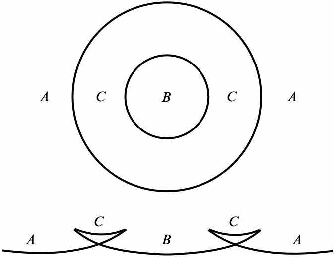
Figure 2: (Figure 17 in [Ekh07]) (Top) The top view of $F_{1}^{\prime}$. (Bottom) The cross-sectional view of $F_{1}^{\prime}$.

We will use the notation in [Ekh07] for (pre)stable flow trees. Vertices will be labelled by Greek letters and edges will be labelled by numbers. For an edge, labelled by $n$, we write $n\coloneqq X|Y$, where $X,Y$ are each one of the four sheets $A,B,C,D$, if the edge $n$ has an associated (broken) gradient flow determined by the sheets $X$ and $Y$.

We will describe our (pre)stable flow trees using the top view of the front $F_{1}^{\prime}$. Consider the sequence of one-edge stable flow trees $T_{\nu}$, with edge $1=A|D$, starting in the region $A$ and flowing horizontally to the region $A$. The sequence $T_{\nu}$ moves this edge downward until it is tangent to the circle connecting the region $C$ to the region $B$. Denote this tangent one-edge stable flow tree by $T$, with edge $1=A|D$. Clearly, $T$ is the Floer-Gromov limit of the sequence $T_{\nu}$. See Figures 3 and 4

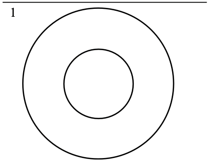
Figure 3: (Figure 18 in [Ekh07]) The sequence of stable flow trees $T_{\nu}$.

Originally, in [Ekh07], the stable flow tree $T$ is described as a two-edge prestable flow tree $\overline{T}$, with a vertex $\alpha$ at the tangency point, and with edges $1=2=A|D$. However, this vertex is a removable vertex (see Remark 3.19).

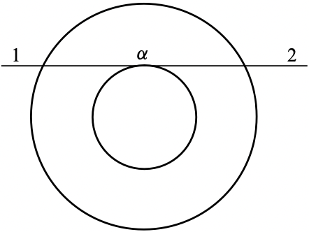
Figure 4: (Figure 19 in [Ekh07]) The original prestable flow tree $\overline{T}$.

Now consider the sequence of four-edge stable flow trees $T_{\nu}^{\prime}$ described as follows. An edge $1=A|D$, flowing from the region $A$ to the region $C$, that ends at a 3-valent vertex $\alpha$. From $\alpha$ we have two other edges: $2=A|C$ flowing transversely into the circle connecting the region $C$ to the region $B$, ending at a vertex $\beta$, and $3=C|D$ flowing tangentially into the circle connecting the region $C$ to the region $B$, that ends at a 2-valent vertex $\gamma$. Finally, from $\gamma$ we have one other edge $4=A|D$, flowing from the region $C$ to the region $A$. The sequence $T_{\nu}^{\prime}$ shrinks the edge 2, colliding the vertices $\alpha$ and $\beta$ into the vertex $\gamma$. See Figure 5.

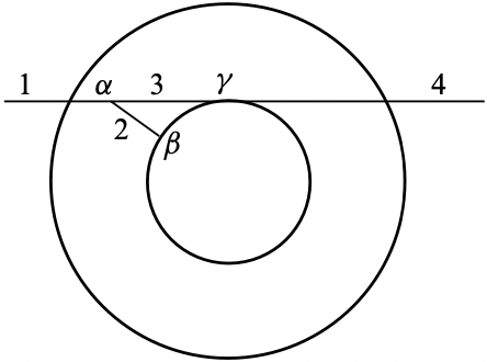
Figure 5: (Figure 20 in [Ekh07]) The sequence of stable flow trees $T_{\nu}^{\prime}$.

The Floer-Gromov limit $T^{\prime}$ of the sequence $T_{\nu}^{\prime}$ will be a stable flow tree, with the same domain as the sequence, where edges 2 and 3 will be ghost edges. In particular, we see that the maps $\lambda:T\to M$ and $\lambda^{\prime}:T^{\prime}\to M$ will have the same image.

Department of Mathematics, Massachusetts Institute of Technology

E-mail address: kblakey@mit.edu

References

- [AD14] Michèle Audin and Mihai Damian. Morse theory and Floer homology. Springer-Verlag, 2014.
- [EENS13] Tobias Ekholm, John Entyre, Lenhard Ng, and Michael Sullivan. Knot contact homology. Geometry and Topology, 17:975–1112, 2013.
- [EES07] Tobias Ekholm, John Entyre, and Michael Sullivan. Legendrian contact homology in . Transactions of the American Mathematical Society, 359(7):3301–3335, July 2007.
- [EGH00] Yakov Eliashberg, Alexander Givental, and Helmut Hofer. Introduction to symplectic field theory. Geometric and Functional Analysis, pages 560–673, 2000.
- [Ekh07] Tobias Ekholm. Morse flow trees and Legendrian contact homology in 1–jet spaces. Geometry and Topology, 11:1083–1224, 2007.
- [EN18] Tobias Ekholm and Lenhard Ng. Higher genus knot contact homology and recursion for colored HOMFLY-PT polynomials. arXiv:1803.04011, March 2018.
- [Flo89] Andreas Floer. Witten’s complex and infinite dimensional Morse theory. Journal of Differential Geometry, 30:207–221, 1989.
- [FO97] Kenji Fukaya and Yong-Geun Oh. Zero-loop open strings in the cotangent bundle and Morse homotopy. Asian Journal of Mathematics, 1(1):96–180, March 1997.
- [MS12] Dusa McDuff and Dietmar Salamon. -holomorphic curves and symplectic topology. American Mathematical Society, 2012.
- [RG19] Georgios Dimitroglou Rizell and Roman Golovko. Legendrian submanifolds from Bohr-Sommerfeld covers of monotone Lagrangian tori. arXiv:1901.08415, January 2019.
- [Riz11] Georgios Dimitroglou Rizell. Knotted Legendrian surfaces with few Reeb chords. Algebraic and Geometric Topology, 11(5):2903–2936, 2011.