Offline Policy Optimization with Eligible Actions

Abstract

Offline policy optimization could have a large impact on many real-world decision-making problems, as online learning may be infeasible in many applications. Importance sampling and its variants are a commonly used type of estimator in offline policy evaluation, and such estimators typically do not require assumptions on the properties and representational capabilities of value function or decision process model function classes. In this paper, we identify an important overfitting phenomenon in optimizing the importance weighted return, in which it may be possible for the learned policy to essentially avoid making aligned decisions for part of the initial state space. We propose an algorithm to avoid this overfitting through a new per-state-neighborhood normalization constraint, and provide a theoretical justification of the proposed algorithm. We also show the limitations of previous attempts to this approach. We test our algorithm in a healthcare-inspired simulator, a logged dataset collected from real hospitals and continuous control tasks. These experiments show the proposed method yields less overfitting and better test performance compared to state-of-the-art batch reinforcement learning algorithms.

1 Introduction

There has been a recent surge in interest, from both the theoretical and algorithmic perspective, in offline/batch Reinforcement Learning (RL). This area could potentially bring insights from RL to the growing number of application settings which produce such datasets (like healthcare [Gottesman et al., 2019, Nie et al., 2021], customer marketing [Bottou et al., 2013, Thomas et al., 2017] or home automation [Emmons et al., 2022]), provide ways to leverage vast amounts of observational training data encoded in videos [Chang et al., 2020, Schmeckpeper et al., 2021], or advance our core understanding of the data characteristics needed to learn near optimal policies.

Many of the settings that might benefit most from offline RL, like healthcare, education or autonomous driving, may not be Markov in the available observed features, and also may not include explicit known representations of the behavior decision policy. This has inspired work on offline policy evaluation estimation methods that make minimal assumptions on the data generation process, such as importance sampling (IS) and doubly robust estimation methods [Precup et al., 2000, Jiang and Li, 2016a, Thomas and Brunskill, 2016] and offline policy learning methods that leverage such estimators [Huang and Jiang, 2020, Cheng et al., 2020, Thomas et al., 2019].

Unfortunately, we show that offline policy selection or learning algorithms that rely on such offline estimation methods that leverage IS can suffer from a key flaw. In brief, the structure of the policy estimator is such that high estimated performance can be achieved both by policies that have high average performance, and by policies that systematically avoid taking actions taken in the dataset for initial states that lead to low rewards. This can substantially inflate the estimated performance of a potential decision policy. As an intuition, consider a setting where some patients arrive much sicker than some healthier patients. In this setting, any policy for the sicker patients will likely yield slightly worse outcomes than the average outcomes for healthier patients, but a policy’s value must be taken in expectation over all patients, not just the healthy patients. We detail how a number of methods, including those that have been proposed before for other reasons, do not solve this issue, including: using a validation set, shifting the reward baseline, and leveraging thresholds on an estimated behavior policy.

Fortunately, we show that a relatively simple method for constraining the policy class considered with off policy learning can greatly ameliorate the problem of propensity overfitting. Our approach can be viewed as related to pessimistic offline RL in Markov decision processes, which has relations to the robust MDP literature [Nilim and El Ghaoui, 2005] and has been receiving growing attention (e.g., Liu et al. [2020], Yu et al. [2020], Kidambi et al. [2020]). One of the key tenants of pessimistic offline RL is to maintain precise quantification over the uncertainty over the model parameters and/or value functions of the Markov decision process, given the available data. A key challenge is how to quantify statistical uncertainty when the state space is extremely large or continuous. This issue is perhaps even more paramount in offline RL settings when we wish to leverage IS-based estimators in order to make minimal assumptions over the data generation process. We show here that constraining the policy class per state only to actions taken in the data for nearby states, which may be viewed as a loose analogy to count-based uncertainty, is sufficient to lower bound the amount of propensity overfitting that can occur. Our approach still ensures asymptotic consistency of the estimation of any policy covered by the behavior policy while providing significant benefits in the finite regime, by essentially constraining policies to observed actions. In this way, our method is related to other methods that revert back to the behavior policy given minimal data for MDP model or value function learning [Satija et al., 2021] or in the bandit setting [Sachdeva et al., 2020, Brandfonbrener et al., 2020]. To our knowledge, our work is the first to explore this for large, non-Markovian stochastic decision processes using policy search methods. We show in simulations and in a real dataset on patient sepsis outcomes that our approach learns policies with significantly higher expected rewards than prior methods, and that those estimates are expected to be reliable, with solid effective samples sizes, a measure of how much of the behavior data would match the proposed policy. Our results highlight and remedy a potential reliability barrier for offline RL with minimal data process and realizability assumptions.

2 Offline Policy Optimization

We study the problem of offline policy optimization in sequential decision-making under uncertainty. Let the environment be a finite-horizon Contextual Decision Process (CDP) [Jiang et al., 2017]. A CDP can capture more general, non-Markovian settings (also sometimes referred to as a Non-Markov DP [Kallus and Uehara, 2019b]). A CDP is defined as a tuple $\langle\mathcal{X},\mathcal{A},H,P,R\rangle$, where $\mathcal{X}$ is the context space, $\mathcal{A}$ is the action space, and $H$ is the horizon. $P=\{P_{h}\}_{h=1}^{H}$ is the unknown transition model, where $P_{h}:(\mathcal{X}\times\mathcal{A})^{h-1}\to\Delta(\mathcal{X})$ is the distribution over next context given the history. $P_{1}:\Delta(\mathcal{X})$ is the initial context distribution. Similarly, $R=\{R_{h}\}_{h=1}^{H}$ is the reward model and $R_{h}:(\mathcal{X}\times\mathcal{A})^{h}\to\Delta([-R_{\max},R_{\max}])$.

In this paper, we focus on learning policies that map from the most recent context to an action distribution, $\pi:\mathcal{X}\to\Delta(\mathcal{A})$. This is optimal when the domain is Markov and can often be more interpretable and more feasible to optimize given finite data in the offline setting. In offline policy optimization settings, we have a dataset with n trajectories collected by a fixed behavior policy $\mu:\mathcal{X}\to\Delta(\mathcal{A})$, and we aim to find a policy $\pi$ in a policy class $\Pi$ with the highest value.

Policy gradient and optimization approaches do not rely on a Markov assumption on the underlying domain, and have had some encouraging success in offline RL  [Chen et al., 2019]. Often these methods leverage an importance sampling (IS) estimator in policy evaluation: $\hat{v}_{\text{IS}}(\pi)=\frac{1}{n}\textstyle\sum_{i=1}^{n}\left(\textstyle\sum_{h=1}^{H}r_{h}^{(i)}\right)\textstyle\prod_{h=1}^{H}\left(\frac{\pi(a^{(i)}_{h}|x^{(i)}_{h})}{\mu(a^{(i)}_{h}|x^{(i)}_{h})}\right).$ The IS estimator is an unbiased and consistent estimate of the value under the following two assumptions:

Assumption 1 (Overlap).

For any $\pi\in\Pi$, and any $x\in\mathcal{X}$, $a\in\mathcal{A}$, $\frac{\pi(a|s)}{\mu(a|s)}<\infty$.

Assumption 2 (No Confounding / Sequential ignorability).

For any policy $\pi\in\Pi$ and $\mu$, conditioning on the current context $x_{h}$, the sampled action $a_{h}$ is independent of the outcome $r_{h:H}$ and $x_{h+1:H}$.

IS often suffers from high variance, which has prompted work into extensions such as doubly robust methods [Jiang and Li, 2016b, Thomas and Brunskill, 2016] and/or methods that balance variance and bias. Truncating the weights and using self-normalization has been shown to be empirically beneficial both in bandit and RL settings [Swaminathan and Joachims, 2015b, Futoma et al., 2020]: we refer to this as Self-Normalized Truncated IS (SNTIS):

$$\textstyle\hat{v}_{\text{SNTIS}}(\pi):=\frac{\sum_{i=1}^{n}\left(\sum_{h=1}^{H}r_{h}^{(i)}\right)\min\left\{\textstyle\prod_{h=1}^{H}W_{h}^{(i)},M\right\}}{\sum_{i=1}^{n}\min\left\{\textstyle\prod_{h=1}^{H}W_{h}^{(i)},M\right\}},$$ (1)

where

$$W_{h}^{(i)}:=\frac{\pi(a^{(i)}_{h}|x^{(i)}_{h})}{\mu(a^{(i)}_{h}|x^{(i)}_{h})}$$ (2)

and $M$ is a constant that truncates the weights. For ease of notation in the rest of this paper, we define:
$W_{1:h}^{(i)}:=\prod_{h=1}^{h}W_{h}^{(i)}$, $W^{(i)}:=W_{1:H}^{(i)}$, $W=\sum_{i=1}^{n}W^{(i)}$, and $r^{(i)}=\sum_{h=1}^{H}r_{h}^{(i)}$.

While this estimate can be used as a direct objective for off policy learning, it may still have a significant variance which is important when comparing across policies. Prior work in contextual bandits [Swaminathan and Joachims, 2015a, Swaminathan and Joachims, 2015b] included a variance penalization in the objective based on the empirical Bernstein’s inequality.

Here we provide a simple extension to the multi-step setting to yield a target objective for offline policy learning:

$$\textstyle\operatorname*{arg\,max}_{\pi\in\Pi}\hat{v}_{\text{SNTIS}}(\pi)-\lambda\sqrt{\widehat{\text{Var}}\left(\hat{v}_{\text{SNTIS}}(\pi)\right)}.$$ (3)

3 Related Work

There is increasing interest in multi-armed bandits and offline RL to avoid overly optimistic estimates of policies computed from finite datasets that can cause suboptimal policy learning. In this paper, we will show a particular unaddressed issue with IS methods avoiding initial states that lead to poor outcomes. In contrast, prior work has shown how to use self-normalized IS (also known as weighted IS) to address over maximizing bandit rewards [Swaminathan and Joachims, 2015b]. Counterfactual risk minimization [Swaminathan and Joachims, 2015a, Joachims et al., 2018] uses variance regularization based on the empirical Bernstein’s inequality for bandit problems. However, this penalization is at the policy level. Both self-normalized IS (SNIS) and variance penalization do not directly solve the problem with avoiding contexts with low reward. In Figure A in Appendix A, we show the counterfactual risk minimization regularization with or without self-normalization requires a large dataset to perform well. Recent work [Brandfonbrener et al., 2020] discussed a similar overfitting issue as we describe and compared the performance of offline policy optimization and model/value-based method on such issue in the bandit setting. Those authors primarily focus on the negative result of the policy optimization approach and the advantage of the model/value-based method, whereas our approach suggests a method for addressing this issue in policy optimization and focuses on the RL setting. Doubly robust estimators [Dudík et al., 2011, Jiang and Li, 2016b, Thomas and Brunskill, 2016, Kallus and Uehara, 2019a, b] have multiple benefits but, as long as the learned $Q$-function is imperfect, the issue of avoiding low performing contexts can still remain as the methods may overfit to the high/positive residual $r-Q$. Pessimism under uncertainty approaches are promising [Kidambi et al., 2020, Yu et al., 2020] but have so far only been developed for Markov settings and are not robust to model class misspecification, unlike IS-based policy optimization.

Another line of offline batch policy optimization constrains the policy search space to be close to the behavior policy, or requires the action taken to have some minimum probability under the behavior policy [Kumar et al., 2019, Buckman et al., 2020, Sachdeva et al., 2020, Fujimoto et al., 2019, Futoma et al., 2020, Liu et al., 2019, 2020]. This work has focused on algorithms and analysis for the Markov setting with additional model realizability and/or closure assumptions that are hard to verify. As we will discuss and empirically validate later, such constraints on the expected or observed empirical behavior policy are not yet sufficient, at least in large state spaces.

Our work can be viewed as following in the recent line of work on pessimism under uncertaintyLiu et al. [2020], Yu et al. [2020], Kidambi et al. [2020], Buckman et al. [2020], but adapted to provide policy search based offline learning method that does not require the Markov assumption or model realizability, and achieves strong performance given a finite dataset.

4 State Propensity overfitting

We identify an important potential issue with using IS estimators during offline policy optimization, as we illustrate in contextual bandits when using the SNIS estimator.

Let $v^{\pi}(x)=\mathbb{E}[r|x,a\sim\pi]$, $\hat{p}(x)$ be the empirical probability mass/density over the contexts $x$ in the dataset, and $W(x)=\sum_{i:x^{(i)}=x}\frac{W^{(i)}}{W}$ where $W$ is the importance weight (Eq. 2). We now decompose the importance weighted off-policy estimator into three parts.

$$\hat{v} =\underbrace{\mathbb{E}_{\hat{p}}[v^{\pi}(x)]}_{\text{empirical }v}+\underbrace{\sum_{x\in\mathcal{X}}(\hat{p}(x)-W(x))v^{\pi}(x)}_{\text{difference in context weights}}$$ (4)

$$+\underbrace{\sum_{x\in\mathcal{X}}W(x)\left(\sum_{x^{(i)}=x}\frac{W^{(i)}}{W(x)W}r^{(i)}-v^{\pi}(x)\right)}_{\text{weighted IS error in each context}}$$ (5)

The first term is a supervised empirical value estimate whose only error is due to the error in the empirical context distribution sampled in the dataset versus the true context distribution. The second term captures the error caused by the difference between context distribution introduced by weights and empirical context distribution in the dataset. The third term computes the difference between the weighted IS estimate of the value of the policy in a specific context $x$ versus its true value $v^{\pi}(x)$, and then sums this over all contexts.

The second term is of particular interest, because it highlights how the IS estimator of a policy may effectively shift the relative weight on the context space. In the bandit setting (and in the initial starting state distribution for RL), such shifting should not be allowed: the policy may control what actions are taken, but cannot change the initial context distribution. We now show how an algorithm maximizing the importance weighted off-policy estimate can exploit this structure and yield overly inflated estimates (Eq. 5).

Example 1.

Consider a contextual bandit problem with $|\mathcal{X}|$ contexts and $|\mathcal{A}|$ actions in each context. For half the contexts $S_{p}$, the reward is $1$ for one action and zero for others. For the other half of the contexts, $S_{n}$, the reward is -1 for half the actions, and -5 for the rest. The true distribution over contexts is uniform. The optimal policy would have an expected reward of 0 over the state space. The behavior dataset is drawn from a uniform distribution over contexts and actions. When the sample size $|\mathcal{D}|<|\mathcal{A}|$, we assume there is only one observed positive reward in the dataset. A policy $\pi_{o}$ that maximizes Eq. 4-5 will select actions that are not present in the dataset for all contexts whose observed actions lead to only zero or negative rewards: let $\mathcal{A}_{s_{i}}=\{a_{i}:r(s_{i},a_{i})\leq 0\}$ then $\pi(s_{i})=a_{j}$ where $a_{j}\notin\mathcal{A}_{s_{i}}$. This will yield $W(x)=0$ on all contexts except for the contexts with observed positive rewards. The resulting IS/SNIS estimator of the value of $\pi_{o}$ is $1$, which is much higher than the optimal value 0. In addition, such a $\pi_{o}$ is likely to be worse than the optimal policy for any context where $r(s_{i},a_{i})=-1$, since that is the optimal reward possible for such states $s_{i}$, and by $\pi$ selecting an unobserved action $a_{j}$ in that state ($\pi(s_{i})=a_{j}$), the policy $\pi$ may select an action with worse true reward, $r(s_{i},a_{j})=-5$.

While this issue can arise in contextual bandits [Swaminathan and Joachims, 2015b], it is even easier for this to occur in sequential RL (Examples 2 and 3 in Appendix A). Intuitively, the issue arises because when estimating the value of a new decision policy, it is acceptable to choose a policy that re-distributes the weights of actions within an initial context but not that re-distributes the weights across initial contexts, since it is not a function of the actions selected. It is well known that in importance sampling, the expected ratio of the weights should be 1: $\mathbb{E}_{y\sim\mu}[\pi(y)/\mu(y)]=1$. In contextual policies, we expect that for each initial context $x_{0}$, the expected weights should also be 1: $\mathbb{E}_{a\sim\mu(a|x_{0})}\left[\pi(a|x_{0})/\mu(a|x_{0})|x_{0}\right]=1$. However, optimizing for a standard importance sampling objective (such as Eq. 5) does not involve constraints that the empirical expectation of weights given an initial context $\hat{\mathbb{E}}[W_{h}^{(i)}|x_{h}^{(i)}]$ (or the weights of $n$-step given initial context $\hat{\mathbb{E}}[W^{(i)}|x_{1}^{(i)}]$ ) is still close to one.

Such propensity overfitting may seem surprising given that under mild assumptions, which are satisfied here by Assumptions 1 and 2, IS provides an unbiased estimate of a policy’s value. Our observations do not contradict this fact: while IS will still provide an unbiased estimate given a policy, policy optimization can exploit the finite sample error and lack of data coverage.

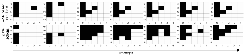
Figure 1: Different policy class constraints in MIMIC sepsis data. The top shows in black which of the 25 actions pass a constraint on having minimal probability over an estimated behavior policy, $\mu_{KNN}(a|s)>b$, for a sequence of patient states. The bottom shows POELA’s eligible actions for the same states. This illustrates that even constraints given the empirical estimated behavior policy can be very different than POELA’s eligible actions. Note sometimes POELA is more conservative, and other times the estimated behavior policy constraint is more conservative.

One might hope that existing methods are sufficient to address this challenge. Here we expand on the discussion in the related work to suggest why this is not the case. First, splitting the data into training and selection sets (e.g., Thomas et al. [2015b], Komorowski et al. [2018]) is generally insufficient. If some of the performance gains come from systematically avoiding actions taken in initial states with low performance, then it is likely that a similar performance benefit can also arise in the validation set if IS-based estimators are used both in policy selection and later estimation. We will observe experimentally this is true even when the estimator or objective involves a variance penalization (Eq. 3). For example, this may occur when only a small set of initial states are avoided, in a way that only mildly impacts the variance and effective sample size, yet results in substantially overly optimistic estimates.

It is also insufficient to shift all rewards to be non-negative. While this voids the benefit of avoiding states if standard IS is used, popular lower-variance IS off-policy estimators like weighted IS are equivariant to any constant shift in rewards. Similarly, doubly robust estimators [Jiang and Li, 2016b, Thomas and Brunskill, 2016] frequently center rewards around estimates of the reward/value outcomes.

Is constraining to the behavior policy sufficient? Perhaps the most compelling idea is whether constraining the policy class to actions with some minimal probability under the behavior policy. First note that constraining to the true behavior policy (e.g., Fujimoto et al. [2019], Sachdeva et al. [2020]) can still cause the propensity overfitting problems we described when the dataset is insufficient to cover all non-zero behavior probability actions in all states. In addition, sometimes the behavior policy is itself unknown. Estimating the behavior policy from data and using this in both the IS-based objective and overlap constraints may be more practical given datasets of limited size and when the state space is large. Indeed, semi-parametric theory and past related work in bandits [Narita et al., 2019] and RL [Hanna et al., 2021] have suggested that even if the behavior policy is known, leveraging the estimated behavior policy can yield more accurate offline policy estimates. It is natural to assume such benefits might also translate to improvements for constrained policy learning.

While promising in principle, this approach may be challenging in large state space environments. First, in such settings the maximum number of observed actions in any particular state is almost always one. Assuming there is good reasons to believe that the behavior policy is not actually deterministic, it is necessary to use some function approximation method to estimate the behavior policy [Hanna et al., 2021], which may be a deep neural network or non-parametric methods like k-nearest neighbors [Raghu et al., 2018]. Unfortunately, as we will demonstrate in our experiments, we find that such approximators may sometimes be sufficient to accurately predict the behavior policy for a given state, but do not seem to be as beneficial when used to constrain the targeted policy class. Such estimates may overestimate (or underestimate) the probability of taking alternate actions in some states, and therefore enable both context avoidance or be too conservative in their policies. Figure 1 illustrates that our method can provide quite different constraints on the policy class than using constraints on the estimated empirical behavior policy, shown for a patient in the MIMIC sepsis dataset.

5 Policy Optimization with ELigible Actions

We have described that in IS-based estimators, because all weight can be placed on unobserved actions for certain initial contexts, the empirical conditional expectation of weights given an initial context $\hat{\mathbb{E}}[W|x]$ can be zero for such contexts, instead of $1$. To address this, one possibility is to constrain the conditional expectation of weights given a context to be $1$ or lower bounded. However doing so in infinite/continuous context spaces is subtle: each context likely only appears once in the dataset, and requiring $\hat{\mathbb{E}}[W|x]=1$ would be equivalent to only allowing a policy that exactly matches the observed logged actions.

We now propose a slight relaxation of the above proposal. Absence constraints, IS-estimator-based policy learning can place a large weight on unobserved actions in the dataset, for which our reward uncertainty is high. The recent line of pessimism under uncertainty for model and value based MDP offline RL (e.g., Liu et al. [2020], Yu et al. [2020]) explicitly accounts for such statistical uncertainty through constraining or penalizing actions and/or states and actions for which there are limited observed data. Our approach is similar but designed to address these issues in settings that may not be Markov.

Specifically, for policy learning, we create local constraints on the eligible policy class. For each context $x$, dataset $\mathcal{D}$ and a given threshold $\delta$, the eligible action set $A(x;\mathcal{D},\delta)$ is:

$$A_{h}(x;\mathcal{D},\delta)\!=\!\{a_{h}:\exists(x_{h},a_{h})\!\in\!\mathcal{D}\,s.t.\,\mathrm{dist}(x,x_{h})\!\leq\!\delta\}.$$

This allows only the action that was taken for a given context, or actions taken in contexts within a given distance $\delta$ of the observed contexts. Note that in large or continuous action spaces, the resulting allowed actions per context may be quite different than policy search methods that places thresholds using the behavior policy probability [Futoma et al., 2020] as we will observe empirically (cf. Figure 1). Intuitively, our eligible action constraint constraints the policy class to observed actions taken in the current or nearby states, but behavior policy thresholds can allow actions that could be taken at that state, even if no such action was taken there, nor at any nearby state. We will shortly prove that our eligible action set is sufficient to lower bound the empirical conditional expectation of weights per observed context. This ameliorates the propensity overfitting problem, and we will shortly show that empirically this can yield significant benefits.

Policy learning can be done by finding the best policy that satisfies the eligible actions constraints given the dataset:

$$\textstyle\operatorname*{arg\,max}_{\pi\in\Pi} \!J(\pi;\mathcal{D})\,$$

$$s.t. \,\forall i,h\,\textstyle\sum_{a\in A_{h}(x_{h}^{(i)};\mathcal{D},\delta)}\!\pi(a|x_{h}^{(i)})\!=\!1.$$ (6)

$J(\pi;\mathcal{D})$ can be any objective function such as $\hat{v}_{\text{IS}}$ or $\hat{v}_{\text{SNTIS}}$.

Algorithm 1 Policy Optimization with ELigible Actions (POELA).

1:Input: $\mathcal{D}$, $\Pi_{\theta}$, sphere radius $\delta$, IS truncation $M$, CRM coefficient $\lambda$, learning rate $\alpha$

2:Output: $\widehat{\pi}_{\theta}$

3:Initialize $\theta_{0}$

4:for $t=0,1$ until convergence do

5:     

$$\widehat{\pi}_{\theta_{t}}(a|x):=\frac{\mathds{1}\{a\in A_{h}(x;\mathcal{D},\delta)\}}{\sum_{a}\mathds{1}\{a\in A_{h}(x;\mathcal{D},\delta)\}\pi_{\theta_{t}}(a|x)}\pi_{\theta_{t}}(a|x)$$

6:     

$$\theta_{t+1}\leftarrow\theta_{t}+\alpha\nabla_{\theta}\left(\hat{v}_{\text{SNTIS}}(\widehat{\pi}_{\theta_{t}})-\lambda\sqrt{\widehat{\text{Var}}\left(\hat{v}_{\text{SNTIS}}(\widehat{\pi}_{\theta_{t}})\right)}\right)$$

7:end for

We now present our POELA (Policy Optimization with ELigible Actions) algorithm (Algorithm 1) that implements the learning objective in Equation 5. We use the counterfactual risk minimization objective function (Eq. 3) as the $J(\pi;\mathcal{D})$, where the estimator $\widehat{\text{Var}}(\hat{v}_{\text{SNTIS}})$ is constructed using the Normal approximation in [Owen, 2013, Equation 9.9]: $\widehat{\text{Var}}(\hat{v}_{\text{SNTIS}})=\frac{\sum_{i=1}^{n}\left(r^{(i)}-\hat{v}_{\text{SNTIS}}\right)^{2}(\min\{W^{(i)},M\})^{2}}{\left(\sum_{i=1}^{n}\min\{W^{(i)},M\}\right)^{2}}.$

After each gradient step, we enforce the policy to satisfy the eligible action constraints by re-normalizing the output probability on $A_{h}(x;\mathcal{D},\delta)$ for $x\in\mathcal{D}$. The eligible action set for each training sample is static and can be stored to reduce computational cost. In the experiments, we use the Euclidean distance over nearby states at any time index.

6 Analysis

In this section we formalize the benefit of the eligible action constraints, and also prove consistency guarantees on the resulting value estimates used in the objective, Equation 5.

Eligible action constraints were introduced to help alleviate propensity overfitting, which can be characterized by the expected empirical sum of propensity weights for a particular context $x$ being much lower than 1, or even $\mathbf{\hat{\mathbb{E}}[W|x]}=0$. We now show that any policy that only selects actions in eligible action sets will ensure that the empirical sum of weights in any hypersphere of any context can be lower bounded, as desired. As mentioned before, for very large state spaces, where only a single action is observed for each observed state in the dataset, the only way to ensure that $\mathbf{\hat{\mathbb{E}}[W|x]}=1$ is to reduce the policy to the observed actions. Intuitively, the guarantee we provide here is reasonable when local smoothness is present and a soft form of state aggregation is tenable, ensuring that the empirical expected sum of weights over nearby states is lower bounded.

To do so, we first introduce an assumption about the target policy’s smoothness in the context space.

Assumption 3 ($L$-Lipschitz policy).

$\forall\pi\in\Pi$, $\|\pi(a|x)-\pi(a|x^{\prime})\|\leq L\mathrm{dist}(x,x^{\prime})$.

That is, nearby contexts have similar actions [Berkenkamp et al., 2017, Wang et al., 2019] which ensures that we have some minimal weight support in a small neighborhood. If different policies have different smoothness, the Lipschitz constant can be taken to be the max over the policy set. Under this assumption and the former assumptions, we can show the following. Proofs are provided in Appendix B:

Theorem 1.

$\forall x_{h}^{(i)}$, $\mathcal{B}(x_{h}^{(i)},\delta):=\{x:\mathrm{dist}(x,x_{h}^{(i)})\leq\delta\}$, $\sum_{x_{h}^{(j)}\in\mathcal{B}(x_{h}^{(i)},\delta)}W_{h}^{(j)}\geq 1-\delta L|\mathcal{A}|$.

Given the likelihood ratio is lower bounded, we can further show that the self-normalized truncated weights are also lower bounded in the one-step settings.

Corollary 1.

For $H=1$, $\sum_{x_{1}^{(j)}\in\mathcal{B}(x_{1}^{(i)},\delta)}\frac{\max\{W^{(i)},M\}}{\sum_{i=1}^{n}\max\{W^{(i)},M\}}\geq\frac{1-\delta L|\mathcal{A}|}{nM}$ for $M>1$.

In the $n$-step sequential setting, it is necessary to have the 1-step weights be greater than zero in order to have $n$-step weights greater than zero.

Proposition 1.

For any $x$, $\delta$, $\mathbb{E}[W_{1:h}^{(i)}|x_{h}^{(i)}\in\mathcal{B}(x,\delta)]=\mathbb{E}[W_{1:h-1}^{(i)}|x_{h}^{(i)}\in\mathcal{B}(x,\delta)]\mathbb{E}[W_{h}^{(i)}|x_{h}^{(i)}\in\mathcal{B}(x,\delta)]$. $\hat{\mathbb{E}}[W_{1:h}^{(i)}|x_{h}^{(i)}\in\mathcal{B}(x,\delta)]=\hat{\mathbb{E}}[W_{1:h-1}^{(i)}|x_{h}^{(i)}\in\mathcal{B}(x,\delta)]\hat{\mathbb{E}}[W_{h}^{(i)}|x_{h}^{(i)}\in\mathcal{B}(x,\delta)].$

The action eligibility local constraints provide a conservative pessimism-like constraint on the policy class, ensuring that the policy does not take actions which have not been tried in nearby states (and therefore for which the potential outcomes are unknown). As we will see shortly, this will yield more stable and beneficial performance in our simulations. An additional desirable property is that asymptotically, POELA relaxes to unconstrained policy learning.

Theorem 2.

(Contains all overlapping policies). For a fixed $\delta$, for any $x$, $A_{h}(x;\mathcal{D},\delta)\to\{a:\mu(a|x)>0\}$ as $n\to\infty$ with probability 1. Therefore asymptotically the policy class will contain all $\pi$ satisfying the overlap assumption.

Theorem 3.

Let $J(\pi,\mathcal{D})$ be the objective in Equation 3, the truncation threshold $M$ as a function satisfies $M\to\infty$ and $M/n\to 0$ as $n\to\infty$, and $|\Pi|<\infty$, then $v^{\hat{\pi}_{\mathcal{D},J}}\to\max_{\pi\in\Pi}v^{\pi}$ in probability.

7 Experiments

	Algorithms	POELA	PO-$\mu$	PO-CRM	BCQ	PQL	$9$-mon
Non-MDP	Test $v^{\pi}$	$95.92\pm 1.68$	$76.99\pm 13.80$	$77.32\pm 14.55$	$13.60\pm 0.15$	$19.64\pm 5.71$	$68.12$
	$\hat{v}_{\text{SNTIS}}-v^{\pi}$	$-1.28\pm 1.93$	$16.07\pm 13.55$	$15.71\pm 14.30$	$80.54\pm 1.42$	$74.48\pm 6.23$	$-$
MDP	Test $v^{\pi}$	$89.53\pm 1.32$	$69.18\pm 10.17$	$63.27\pm 13.27$	$82.68\pm 15.19$	$99.98\pm 0.38$	$68.12$
	$\hat{v}_{\text{SNTIS}}-v^{\pi}$	$5.12\pm 2.01$	$24.92\pm 9.71$	$30.82\pm 12.59$	$14.76\pm 14.89$	$-2.65\pm 1.76$	$-$

Table 1: LGG Tumor Growth Inhibition simulator. Test $v^{\pi}$ (1000 rollouts in the simulator) and $\hat{v}_{\text{SNTIS}}-v^{\pi}$ (amount of overfitting of the learned policy) with $\hat{v}_{\text{SNTIS}}$ on the validation set. Average across 5 runs with standard error reported.

We now compare POELA with several prior methods for offline RL. Perhaps the most relevant work in avoiding overfitting when using importance sampling is norm-POEM [Swaminathan and Joachims, 2015b]. For it to be suitable for sequential decision settings, we use a neural network policy class and refer to the resulting algorithm as PO-CRM. A second baseline PO-$\mu$ constrains the policy class to only include policies which take actions with a sufficient probability under the behavior policy $\mu(a|s)$ [Futoma et al., 2020]. We also compare with recent deep value-based MDP methods in batch RL: BCQ [Fujimoto et al., 2019] and PQL [Liu et al., 2020]. For all algorithms, we use a feed-forward neural network for the relevant policy and/or value function approximators. We report the test performance of the selected policy either through online Monte-Carlo estimation if a simulator is available, or using SNTIS estimates on a held out test set. Full details are provided in Appendix C.

7.1 Tumor Inhibition Simulator

The Tumor Growth Inhibition (TGI) simulator [Ribba et al., 2012] describes low-grade gliomas (LGG) growth kinetics in response to chemotherapy in a horizon of 30 steps (months), with a non-Markov context and a binary action of drug dosage [Yauney and Shah, 2018]. The reward is an immediate penalty proportional to the drug concentration, and a delayed reward of the decrease in mean tumor diameter. The behavior policy selects from a fixed dosing schedule of 9 months (the median duration from Peyre et al. [2010]) with 70% probability and else selects actions at random.

In this experiment, the behavior policy can only take values in $\{0.15,0.85\}$. This means that constraining the policy class to have a minimal probability under $\mu(a|s)$, as in baseline PO-$\mu$, is only a non-trivial constraint for thresholds greater than $0.15$: this generates a single potential target policy, which is the deterministic fixed-dosage part of behavior policy. We include this as $9$-mon (short for 9 month dosing) in Table 1. The training and validation sets both have 1000 episodes. We repeat the experiment 5 times with 5 different train and validation sets. Policy values are normalized between $0$ (uniform random) and $100$ (best policy from online RL). As shown in Table 1 (Non-MDP rows), POELA achieves the highest test value as well as smaller variability compared with the baselines.

Does POELA reduce overfitting? Examining the difference between $\hat{v}_{\text{SNTIS}}$ on the validation set and the online test value, we observe that most algorithms result in a policy whose value is a significant overestimate of its true performance (cf. Table1, $\hat{v}_{\text{SNTIS}}-v^{\pi}$). In contrast, POELA yields a policy whose value is much more accurately estimated and performs better. Experiments with final policies selected during training based on SNTIS estimates on the validation set suggest the same conclusion (cf. Table 12 in Appendix D.2).

Performance comparison in a MDP environment. We also repeat the experiment with an MDP modification of the simulator, including an immediate Markovian reward and additional features for a Markovian state space. Note that we expect BCQ and PQL to do very well: both are designed to avoid overfitting in offline MDP learning and in particular PQL uses a pessimism under uncertainty approach to penalize policies that put weight on state-action pairs with little support. Although POELA makes no Markov assumptions, it ponly erforms on average slightly worse than the two conservative MDP methods but still outperforms BCQ. POELA also substantially outperforms other policy classes.

Method	POELA	PO-$\hat{\mu}$	PO-CRM	BCQ	PQL	Clinician
Test SNTIS	92.32 (90.87)	90.21	86.89	25.62	27.04	81.10
$95\%$ BCa UB	95.83 (92.94)	93.27	89.68	41.93	42.45	82.19
$95\%$ BCa LB	90.91 (87.22)	87.19	83.50	7.93	13.43	79.80
Test ESS	437.03 (396.71)	297.84	289.10	206.63	217.54	2995

Table 2: MIMIC III sepsis dataset. Test evaluation, $(0.05,0.95)$ BCa bootstrap interval, and ESS. The value of POELA without a CRM variance penalty is in parentheses.

Method	POELA	PO-$\hat{\mu}$	PO-CRM	BCQ	PQL
Test SNTIS	86.42 (85.26)	84.39	79.71	32.83	34.69
$95\%$ BCa UB	91.68 (90.32)	87.74	89.33	53.50	52.15
$95\%$ BCa LB	79.71 (77.15)	80.01	65.01	11.87	17.60
Test ESS	310.23 (287.39)	244.97	224.92	207.12	223.03

Table 3: Idem except using behavior policy $\hat{\mu}=\text{BC}$.

Method	POELA	PO-$\hat{\mu}$	PO-CRM	BCQ	PQL
Test SNTIS	88.83 (88.31)	87.97	85.33	33.21	41.66
$95\%$ BCa UB	93.23 (94.04)	91.17	89.44	63.17	57.99
$95\%$ BCa LB	83.43 (80.02)	82.00	78.43	12.23	14.76
Test ESS	379.18 (265.36)	220.74	236.78	203.89	224.33

Table 4: Idem except using behavior policy $\hat{\mu}=\text{BCRNN}$.

7.2 MIMIC III Sepsis ICU data

Next, we apply our method in a real-world example of learning policies for sepsis treatment in medical intensive care units (ICU). We used an extracted cohort [Komorowski et al., 2018] of patients fulfilling the sepsis-3 criteria from the MIMIC III data set [Johnson et al., 2016] and obtained a dataset of 14971 patients, 44 context features, 25 actions and a 20 step maximum horizon. Full details are in the Appendix C.2. We hold out $20\%$ of data for validation and $20\%$ of data for the final test. Treatment logs do not include the probabilities of clinicians’ actions. Instead, as suggested by prior work [Raghu et al., 2018], we estimate the probabilities of the behavior clinicians’ policy by $k$-NN with $k=100$. To ensure overlap, for all policy optimization algorithms we allow $\pi(a|s)>0$ only if $\hat{\mu}(a|s)>0$. Using SNTIS to evaluate the performance on a test set is appealing because it makes little assumptions on the underlying domain. But if only a few test behavior policy trajectories match a test policy, the resulting value estimate is likely unreliable. We measure the amount of overlap between the test set and a desired policy by the effective sample size (ESS) [Owen, 2013]. Only policies with an ESS of at least $200$ on the validation set are considered.Similar to prior work [Thomas et al., 2015a], in addition to the SNTIS estimator on the test set, we also report a $95\%$ upper and lower bound from bias-corrected and accelerated (BCa) bootstrap. The clinician’s column is the test dataset rewards and sample size.

Table 2 shows POELA is the best on all metrics, achieving the highest evaluation on the test set, the highest upper and lower bounds, and the highest ESS. We also show that POELA’s test performance without its variance penalty is worse than using it but is still higher than the baseline algorithms. In Appendix E.3, we further detail the differences in the methods under the prism of ESS and performance. We also demonstrate in Appendix E.4 that POELA takes actions which more closely match the clinicians’ actions for patients with initially high logged SOFA scores (measuring organ failure) in the test dataset in comparison to other baselines, suggesting that propensity overfitting may be occurring more in other methods. Finally, Figure 1 illustrates different actions constraints considered in this paper, using a sample trajectory in the test set as an example, where the 25 actions are depicted in 5x5 grids.

7.3 Behavior policy Estimation

We now explore further if constraining policies to be close to the empirical behavior policy may produce similar benefits, and whether this depends on the function approximator used. We consider two additional function approximators: (1) learning a deep neural network representation of the behavior policy using Behavior Cloning (BC), an imitation learning approach [Pomerleau, 1991] and (2) training a recurrent neural network behavior representation using BCRNN, a variant of BC with a RNN as the policy network. BCRNN can learn temporal dependencies, which can be helpful. More details are included in Appendix C.3.

Results in the MIMIC III sepsis dataset are shown in Tables 4 and 4. Results in the Tumor simulator are included in Tables 10 and 11. Overall, this behavior policy modelling modification impacts all methods, but POELA still outperforms other baselines. We note that BCQ and PQL benefit from these alternate behavior policy approximators, while policy-based methods suffer from it in the Non-MDP setting. Comparing the benefits of using BC versus BCRNN, BCRNN behavior policy approximators in the non-Markov settings generally helps, as expected. We report additional results where best policies are selected from checkpoints during training based on SNTIS estimates in Tables 13 and 14 (tumor) and in Tables 16 and 17 (sepsis). In this application-driven selection procedure, POELA still yields higher test values.

7.4 Experiment with continuous state space

In the next experiment, we use the OpenAI Gym environment [Brockman et al., 2016] CartPole. We also apply our method to a non-Markov modification of the environment. More details about this experiment in Appendix F. In these experiments, only policies with an ESS of at least $30$ on the validation set are considered. Because of space constraints, the full results are provided in Appendix F. Tables 20 to 23 show the results. We observe that in both MDP and Non-MDP settings, POELA provides improved performance over other methods. We also provide some results on D4RL [Fu et al., 2020] datasets in Appendix G. These results show that relying on observed data to decide on action eligibility can be beneficial for learning from the relatively few number of trajectories collected by the behavior policy in a continuous state space.

8 Discussion & Conclusion

A natural question is whether POELA, in addition to its overall improved performance, reduces context avoidance/propensity overfitting in practice. In Appendix C.4, we find that POELA generally puts more weight on initial states with low observed outcomes than other IS policy optimization methods, suggesting that it addresses the motivating problem. POELA also does not seem highly sensitive to the threshold used in the eligible action constraint (cf. Appendix C.5) although middle ranges are more effective.

An alternative to constrained optimization is a soft penalty based on the proportion of contexts that are avoided through selecting alternative actions. This idea was previously proposed for contextual bandits [Sachdeva et al., 2020]. This is challenging to approximate in the RL setting, where deficiency can occur at any steps in a trajectory: exploring this is an interesting area for future work. Another interesting direction is to adapt the solution found in Joachims et al. [2018] when using a minibatch biases the SNTIS estimate.

To conclude, we identify a new overfitting problem arising when using IS as part of an offline policy learning objective. To address this, we constrain the policy class to only consider logged actions taken by nearby states. This can be viewed as a pessimism constraint similar to the one used in MDP offline policy learning, but developed for a non-Markov, direct policy search setting. Our approach yields strong performance relative to state-of-the-art approaches in a tumor growth simulator, a real-world dataset on ICU sepsis treatment and in classic continuous control with few demonstrations. POELA may be particularly useful for many applied settings such as healthcare, education and customer interactions, which have a short/medium length decision horizon, but are unlikely to be Markov in the observed per-step variables. Leveraging constraints on an empirical behavior policy was not as helpful, but an interesting direction for future work is whether other ways of learning such behavior policy might yield additional benefits to our locally constrained approach.

We first briefly describe the structure of the Appendix here. In Appendix A we add two more examples in the multi-step settings as supplementary to the example in Section 4. In Appendix B we provide the proofs of theorems in Section 6. In Appendix C, we include more experiment details. In Appendices D, E, F and G we include more results in the considered domains including experiments with estimating the behavior policy with function approximation and experiments with an alternative policy selection procedure with best intermittent policy checkpoint and the D4RL dataset. In the real world dataset on ICU sepsis treatment, we also include in Appendix E.2 an ablation study without ESS constraints for hyperparameter selection on the validation set and in Appendix C.5 an investigation of the effect of eligible action constraints $\delta$. In AppendixC.4 we also investigate the the weight given by different methods to states with low observed outcomes, and we conduct experiments on the differences in the methods under the prism of ESS and performance in Appendix E.3. Finally, in Appendix E.4 we include visualizations of eligible actions for high/mid/low-SOFA patients in addition to a timestep-by-timestep visualization of the two action constraints considered in this paper (based on the eligible action set in POELA and based on the probability under the behavior policy for other methods).

Appendix A Counter Examples in RL Settings

In the main text, we gave an example about the overfitting issue in contextual bandits with large state and action space in small datasets. Here we show that it is even easier for this to occur in sequential reinforcement learning settings, even when only 2 actions are available in the next two examples with or without state aliasing.

Example 2.

Consider a sequential treatment problem as shown in Figure A. There are two actions available in each state. From the first state, action $a_{1}$ has a 50% chance of leading to an immediate terminal positive reward $r=1$ and a 50% chance of leading to an immediate terminal negative reward $r=-1$. From the first state, action $a_{2}$ also has 50% chance of leading to an immediate terminal positive reward $r=1$. For the other 50% of states, action $a_{2}$ results in transitions to additional states, which are followed by additional actions, for another $H-1$ steps; however, all transitions eventually end in a large negative outcome (e.g., $r=-5$). For example, one could consider a risky surgical procedure that results in many subsequent additional operations and but is ultimately typically unsuccessful. Assume the behavior policy is uniform over each action, yielding $\mu(a=0|x_{1})=\mu(a=1|x_{1})$ = 0.5 and a probability of each action sequence following $a_{2}$ of $\frac{1}{|A|^{H-1}}$. With even minimal data the value of $\pi(x_{0})=a_{1}$ will be accurately estimated as 0. However, when $H$ is large relative to a function of the dataset size, there always exists a action sequence after an initial selection of $a_{2}$ that is not observed in the dataset. This means that a policy $\pi_{2}$ that starts with $\pi(x_{0})=a_{2}$ and then selects an unobserved action sequence will essentially put 0 weight on the resulting contexts that incur $r=-5$ outcomes, even though such outcomes will occur 50% of the time after taking action $a_{2}$. In this case, the value of $\pi_{2}$ will be overestimated significantly by IS or self-normalized IS. Thus the offline policy optimization will prefer taking action 2 at the first step as a result of overfitting even though the true value of first taking $a_{2}$ is $-1.5$ and the optimal policy value is $0$, obtained by taking action $a_{1}$.

Now we add a slight change in the transitions shown in Figure A. We can see that model/value-based approach will also fail.

Example 3.

In this example, we add another action in the first step. The action $3$ and action $1$ will lead to the same next state. However in the next state, no matter which action taken, the reward will depends on the action taken in the last step: If $a_{1}=1$, then we have the same reward for $a=1$ in the example in Figure A. If $a_{1}=3$ then we have a reward $-5$. Thus model and value based method will mix the reward for $a_{1}=1$ and $a_{1}=3$ so fail in this example. Other method is not affected by the additional structure as it only add an action with minimum reward.

(a) Example 2.

(b) Example 3.

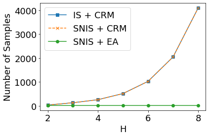
(c) Number of samples to solve Example 2/3 for $A=2$.

Appendix B Proofs of Section 6

Proof of Theorem 1.

Proof.

$$\sum_{x_{h}^{(j)}\in\mathcal{B}(x_{h}^{(i)},\delta)}\frac{\pi(a_{h}^{(j)}|x_{h}^{(j)})}{\mu(a_{h}^{(j)}|x_{h}^{(j)})}\geq \sum_{x_{h}^{(j)}\in\mathcal{B}(x_{h}^{(i)},\delta)}\pi(a_{h}^{(j)}|x_{h}^{(j)})$$ (7)

$$\geq \sum_{x_{h}^{(j)}\in\mathcal{B}(x_{h}^{(i)},\delta)}\max\{0,\pi(a_{h}^{(j)}|x_{h}^{(i)})-\delta L\}$$ (8)

$$\geq \sum_{a\in A_{h}(x_{h}^{(i)};\mathcal{D},\delta)}\max\{0,\pi(a|x_{h}^{(i)})-\delta L\}=1-\delta L|\mathcal{A}|$$ (9)

∎

Proof of Corollary 1.

Proof.

$$\sum_{x_{1}^{(j)}\in\mathcal{B}(x_{1}^{(i)},\delta)}\frac{\max\{W^{(i)},M\}}{\sum_{i=1}^{n}\max\{W^{(i)},M\}} \geq\sum_{x_{1}^{(j)}\in\mathcal{B}(x_{1}^{(i)},\delta)}\frac{\max\{W^{(i)},M\}}{nM}$$ (10)

$$\geq\frac{\max\{\sum_{x_{1}^{(j)}\in\mathcal{B}(x_{1}^{(i)},\delta)}W^{(i)},M\}}{nM}$$ (11)

$$\geq\frac{1-\delta L|\mathcal{A}|}{nM}$$ (12)

∎

Proof of Proposition 1.

Proof.

This is due to $\pi(a|x_{h}^{(i)})$ and $\mu(a|x_{h}^{(i)})$ are independent from history given $x_{h}^{(i)}$. So $W_{1:h}^{(i)}$ and $W_{h}^{(i)}$ are conditionally independent given $x_{h}^{(i)}$. ∎

Proof of Theorem 2.

Proof.

Let $\mathrm{P}_{h}(x;\mu)$ to be the distribution of context at $h$-th step with roll-in policy $\mu$. For any fixed $a$, we can define the distribution $\mathrm{P}_{h}(x|a;\mu)=\mu(a|x)\mathrm{P}_{h}(x;\mu)/\sum_{a}\mu(a|x)\mathrm{P}_{h}(x;\mu)$. For $a$ such that $\mu(a|x)>0$, $\mathrm{P}_{h}(x|a;\mu)$ is also greater than zero. All $x_{h}^{(i)}$ with $a_{h}^{(i)}=a$ are i.i.d. samples draw from the distribution $\mathrm{P}_{h}(x;\mu)$. By the property of nearest neighbor [Cover and Hart, 1967], with probability 1:

$$\min_{x_{h}^{(i)}s.t.a_{h}^{(i)}=a}\mathrm{dist}(x,x_{h}^{(i)})\to 0<\delta.$$

That means with probability $1$ $a\in A_{h}(x;\mathcal{D},\delta)$ for all $a$ such that $\mu(a|x)>0$. Thus we proved the theorem statement and that the policy class will contain all $\pi$ such that $\pi(a|x)>0$ if $\mu(a|x)>0$. ∎

Proof of Theorem 3.

Proof.

Given the overlap assumption and Theorem 2, for all $\pi$ we have $a\in A_{h}(x;\mathcal{D},\delta)$ for all $a$ such that $\pi(a|x)>0$ with probability 1. Thus the solution to Equation 5 is the same as $\operatorname*{arg\,max}_{\pi}J(\pi,\mathcal{D}):=\hat{\pi}_{J,\mathcal{D}}$.

By the condition that $M\to\infty$ and $\frac{M}{n}\to 0$ as $n\to\infty$, we have that the truncated IS estimator is mean square consistent [Ionides, 2008]:

$$\frac{1}{n}\sum_{i=1}^{n}\left(\sum_{h=1}^{H}r_{h}^{(i)}\right)\min\left\{\prod_{h=1}^{H}W_{h}^{(i)},M\right\}\xrightarrow[]{q.m.}v^{\pi},$$ (13)

as $n\to\infty$. Similarly, we have that the mean of weights converge to $1$ in quadratic mean:

$$\frac{1}{n}\sum_{i=1}^{n}\min\left\{\prod_{h=1}^{H}W_{h}^{(i)},M\right\}\xrightarrow[]{q.m.}1.$$ (14)

By continuous mapping theorem, we have that the self-normalized truncated IS converge to $v^{\pi}$ in probability $\hat{v}_{\text{SNTIS}}\xrightarrow[]{p}n$. The empirical variance penalty, also converge to $0$ almostly surely, since $M/n$ converge to $0$:

$$\frac{\sum_{i=1}^{n}\left(r^{(i)}-\hat{v}_{\text{SNTIS}}\right)^{2}(\min\{W^{(i)},M\})^{2}}{\left(\sum_{i=1}^{n}\min\{W^{(i)},M\}\right)^{2}}\leq\frac{M^{2}}{\left(\sum_{i=1}^{n}\min\{W^{(i)},M\}\right)^{2}}\xrightarrow[]{q.m.}0.$$ (15)

Thus the objective function $J(\pi;\mathcal{D})$ converge to $v^{\pi}$ in probability:

$$\Pr\left(|J(\pi;\mathcal{D})-v^{\pi}|>\epsilon\right)=\delta_{n}\to 0.$$ (16)

Since we assume $|\Pi|<\infty$, we have

$$\Pr\left(\forall\pi\in\Pi\,|J(\pi;\mathcal{D})-v^{\pi}|>\epsilon\right)=|\Pi|\delta_{n}.$$ (17)

So with probability $|\Pi|\delta_{n}$, for any $\epsilon$:

$$v^{\hat{\pi}_{J,\mathcal{D}}}\geq J(\hat{\pi}_{J,\mathcal{D}},\mathcal{D})-\epsilon$$ (18)

$$\geq J(\pi^{\star},\mathcal{D})-\epsilon$$ (19)

$$\geq v^{\pi^{\star}}-2\epsilon,$$ (20)

where $\pi^{\star}$ is $\operatorname*{arg\,max}_{\pi\in\Pi}v^{\pi}$. As $|\Pi|\delta_{n}\to 0$, we proved the true value of empirical maximizer $v^{\hat{\pi}_{J,\mathcal{D}}}$ converge to the maximum of value $\max_{\pi\in\Pi}v^{\pi}$ in probability. ∎

Appendix C Experiment Details

For all experiments in the main text, we report the test performance of the policy saved at the end of training either through online Monte-Carlo estimation if a simulator is available, or using SNTIS estimates on a held out test set.

For all experiments reported in Appendices D.2 and E.1, we follow the 3-phases pipelines we describe hereafter to decide the test score we report in the corresponding Tables. To put ourselves in the more realistic situation of real-world applications where practitioners would select a policy from regular checkpoints along its training on the basis of its SNTIS score on the validation set, an algorithm is trained on the training set multiple times, using different hyperparameters and several restarts. Intermittent policies generated during the training process identified with the highest self-normalized truncated IS (SNTIS) estimates on a held-out validation set are saved at checkpoints. The pipeline is illustrated in Figure 2.

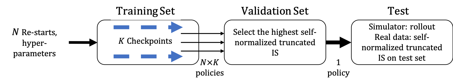
Figure 2: The process of hyperparameters search and test in the experiment.

The open-source code for POELA can be found here: https://github.com/StanfordAI4HI/poela.

C.1 Experiment Details in TGI Simulator

The TGI simulator describes low-grade gliomas (LGG) growth kinetics in response to chemotherapy in a horizon of 30 months using an ordinary differential equation model. The parameter in ODEs are estimated using data from adult diffuse LGG during and after chemotherapy was used, in a horizon of 30 months. The goal in this environment is to achieve a reduction in mean tumor diameters (MTD) while reducing the drug dosage [Yauney and Shah, 2018]. We includes the MTD, the drug concentration, and the number of month (time-step) in the context space. Notice that this context space is non-Markov as it does not include all parameters in the ODEs. Actions are binary representing taking the full dose or no dose which is same as prior work [Yauney and Shah, 2018]. The reward at each step consist of an immediate penalty proportional to the drug concentration, and a delayed reward at the end measures the decrease of MTD compared with the beginning. Each episodes, the parameters including the initial MTD are sampled from a log-Normal distribution as [Ribba et al., 2012] representing the difference in individuals. The behavior policy is a fixed dosing schedule of 9 months (the median duration from Peyre et al. [2010]) plus $30\%$ of a uniformly random choice of actions. We run all algorithms on a training set with 1000 episodes with different hyperparameters (listed below), and 5 restarts, saving checkpoints along the training.The validation set is comprised of 1000 episodes as well.

Hyperparameters.

In the first part of Table 5 we show the searched hyperparameters of each algorithm, except that the parameter $b$ in PQL is set adaptively as the $2$-percentile of the score on the training set as in the original paper Liu et al. [2020]. As we know the behavior policy, we use the true behavior policy in BCQ and PQL algorithm. So BCQ threshold takes only two values as the behavior policy is $\epsilon$-deterministic so there are only two distinct values. In the second part of Table 5 we specify some fixed hyperparameters/settings for all algorithm. All policy/Q functions are approximated by fully-connected neural networks with two hidden layers with 32 units.

Hyperparameters	used in algorithms	values
$\delta$	POELA	$0.05,0.1,0.5$
$\hat{\mu}$ threshold	PO-$\mu$	0.01, 0.05, 0.1, 0.2
CRM Var coefficient	POELA, PO-CRM	$0,0.1,1$
BCQ threshold	BCQ, PQL	$0.0,0.2$
$M$ in $\hat{v}_{\text{SNTIS}}$	All	$1000$
Max training steps	POELA, PO-CRM, PO-$\mu$	500
	BCQ, PQL	1000
Number of checkpoints	All	50
Batch size	BCQ, PQL	100

Table 5: Hyperparameters in the TGI simulator experiment

The difference in the max update steps and checkpoints frequency is caused by the fact that BCQ and PQL is updated by stochastic gradient descent and all policy optimization based on SNTIS is using gradient descent.

C.2 Experiment Details in the MIMIC III Dataset

The MIMIC III sepsis dataset is available upon application and training: https://mimic.mit.edu/iii/gettingstarted/. The code to extract the cohort is available on: https://gitlab.doc.ic.ac.uk/AIClinician/AIClinician. This cohort consists of data for 14971 patients. The contexts for each patient consist of 44 features, summarized in 4-hour intervals, for at most 20 steps. The actions we consider are the prescription of IV fluids and vasopressors. Each of the two treatments is binned into 5 discrete actions according to the dosage amounts, resulting in 25 possible actions. The rewards are defined from the 90-day mortality in the logs, $100$ if the patient survives and $0$ otherwise.

We now provide details of the experiment on MIMIC III sepsis dataset here. We run all algorithms on a training set with 8982 trajectories with different hyperparameters (listed below), and 3 restarts, saving checkpoints along the training.The validation set is comprised of 2994 trajectories. Finally we get the $\hat{v}_{\text{SNTIS}}$ evaluation on the test set with 2995 trajectories. In the first part of Table 6 we list the hyperparameters that we searched on the validation set for each algorithm, except that the parameter $b$ in PQL is set adaptively as the $2$-percentile of the score on the training set as in the original paper [Liu et al., 2020]. In the second part of Table 5 we specify some fixed hyperparameters/settings for all algorithm. All policy/Q-functions are approximated by fully-connected neural networks with two hidden layers with 256 units.

Hyperparameters	used in algorithms	values
$\delta$	POELA	$0.4,0.6,0.8,1.0$
$\hat{\mu}$ threshold	PO-$\mu$	0.01, 0.02, 0.05, 0.1
CRM Var coefficient	POELA, PO-CRM	$0,0.1,1,10$
BCQ threshold	BCQ, PQL	$0.0,0.01,0.05,0.1,0.3,0.5$
$M$ in $\hat{v}_{\text{SNTIS}}$	All	$1000$
Max training steps	POELA, PO-CRM, PO-$\mu$	1000
	BCQ, PQL	10000
Number of checkpoints	All	100
Batch size	BCQ, PQL	100

Table 6: Hyperparameters in the MIMIC III sepsis experiment

As we explained, the difference in the max update steps and checkpoints frequency is caused by the fact that BCQ and PQL is updated by stochastic gradient descent and all policy optimization based on SNTIS is using gradient descent.

C.3 Experiment Details for the Behavior policy Estimation

In the implementation of BC, we use Multi-Layer Perceptrons (MLPs) neural networks with layer dimensions [32, 32, 32] for the LGG Tumor Growth Inhibition simulator and [256, 256, 256] for the MIMIC III dataset. All use ReLU activations. For BCRNN, we use 3-layer GRUs with a RNN hidden dimension of size 100. All networks are trained using Adam optimizer [Kingma and Ba, 2014] with learning rate $3e-4$. For all experiments, BC and BCRNN are trained for 500 steps and directly serve as estimated behavior policies.

C.4 Importance weights in low-reward trajectories

To examine if the proposed overfitting phenomenon exists in real experimental datasets, we compute the importance weights of the learned policy on the low-reward trajectories in the training data for our MIMIC III dataset and our tumor simulator. Our hypothesis is that overfitting of the importance weights in policy gradient methods may result in the algorithm avoiding initial states with low rewards, which motivated our proposed algorithm.

In MIMIC III dataset the reward for a trajectory is either $0$ or $100$. We define the low-reward trajectories as those with $0$ reward. Low-reward trajectories are over $60\%$ of all trajectories in the dataset. In the Tumor simulation experiment we define a low-reward trajectory when reward is less than $-2$. Over $95\%$ of trajectories in the Tumor simulation dataset are low-reward trajectories.

The table below shows, for each algorithm and setting, the sum of the SNTIS weights of the learned policy on the training set, for low-reward trajectory states. Our primary interest is to illustrate that alternate policy gradient methods that are also suitable for non-Markov domains, can exhibit the importance sampling overfitting of avoiding low reward trajectories. We indeed see in Table 7 that POELA has a much larger weight on low-reward trajectories than alternate offline policy search methods:

Method	POELA	PO-$\mu$	PO-CRM
MIMIC III	0.028	0.001	0.003
Tumor non-MDP	0.054	- (fixed policy)	0.005

Table 7: Importance weights overfitting: sum of SNTIS weights of learned policy on the training set.

The Q-learning baselines we consider (BCQ and PQL) do not directly use the importance weights, but they do try to avoid actions and/or states and actions with little support. Our POELA method can be viewed as being similarly inspired, but for non-Markovian settings where policy gradient is beneficial. We also compute the SNTIS weights of the BCQ/PQL policy on the training set in the Markov domain that satisfies the Markov assumptions of BCQ/PQL. In Table 8 we can see that POELA, BCQ and PQL all still give significantly more weight to low reward trajectories than the alternate policy gradient methods:

Method	POELA	PO-$\mu$	PO-CRM	BCQ	PQL
Tumor MDP	0.097	- (fixed policy)	0.0004	0.083	0.124

Table 8: Importance weights overfitting: sum of SNTIS weights of learned policy on the training set.

These results help illustrate that the over avoidance of low-reward trajectories can be observed by past policy gradient methods in our datasets. Of course, one challenge is that in real settings, an excellent policy may have low importance weights in avoidable low-reward states and trajectories, but should have higher importance weights in non-avoidable low reward starting states and trajectories. To get a fuller picture of performance, it is helpful to look both at the weights on trajectories with low rewards and the test evaluation results. Compared with strong policy gradient baselines, our proposed regularization method have larger importance weights on low-reward trajectories, and the gap between training/validation evaluation and online test performance is also smaller, suggesting that we are less likely to learn policies that erroneously believe they can avoid unavoidable low reward settings.

C.5 The effect of eligible action constraints $\delta$

In this section we explore how the choice of $\delta$, which constrains the policy class through impacting the eligible actions, impacts empirical performance. Larger $\delta$ corresponds to a less constrained policy class. Other hyperparameters are selected by the same procedure as described in previous sections.

Table 9 shows the results. As $\delta$ increases, the policy search operates with less constraints. The results show that in this case, our policy gradient method produces a policy with a higher value in the training set, but that policy may not perform as well in the test evaluation, and may have a smaller effective sample size than when a smaller $\delta$ is used. The best hyperparameter value $\delta$ lies in the middle of the explored range. $\delta$ can be selected based on performance and effective sample size.

$\delta$	0.4	0.6	0.8	1.0
training $\hat{v}_{\text{SNTIS}}$	91.62	98.41	98.9	99.12
training ESS	3601.12	2242.07	1993.08	1769.46
test $\hat{v}_{\text{SNTIS}}$	86.62	90.07	91.46	90.23
test ESS	1278.08	819.64	624.92	542.53

Table 9: The effect of eligible action constraints $\delta$ on the results in MIMIC III sepsis dataset.

Appendix D Additional experiments: LGG Tumor Growth Inhibition simulator

In this section, we provide additional experiments to the existing LGG Tumor Growth Inhibition simulator experiments.

D.1 Experiment with estimating the behavior policy with function approximation

	Algorithms	POELA	PO-$\hat{\mu}$	PO-CRM	BCQ	PQL	$9$-mon
Non-MDP	Test $v^{\pi}$	$92.34\pm 1.57$	$59.62\pm 12.71$	$46.66\pm 14.05$	$19.36\pm 5.66$	$30.44\pm 10.38$	$68.12$
	$\hat{v}_{\text{SNTIS}}-v^{\pi}$	$0.94\pm 1.66$	$31.38\pm 10.97$	$42.98\pm 12.87$	$72.35\pm 5.66$	$62.24\pm 10.94$	$-$
MDP	Test $v^{\pi}$	$91.04\pm 0.55$	$78.21\pm 4.94$	$78.70\pm 0.60$	$99.26\pm 0.59$	$99.66\pm 0.29$	$68.12$
	$\hat{v}_{\text{SNTIS}}-v^{\pi}$	$3.40\pm 2.48$	$15.58\pm 3.92$	$15.10\pm 3.97$	$-3.88\pm 1.60$	$-4.09\pm 1.75$	$-$

Table 10: LGG Tumor Growth Inhibition simulator. Test $v^{\pi}$ and amount of overfitting of the learned policy. Test $v^{\pi}$ is computed from 1000 rollouts in the simulator. $\hat{v}_{\text{SNTIS}}$ on the validation set $-$ test $v^{\pi}$ represents the amount of overfitting. All numbers are averaged across 5 runs with the standard error reported. Behavior policy $\hat{\mu}=\text{BC}$.

	Algorithms	POELA	PO-$\hat{\mu}$	PO-CRM	BCQ	PQL	$9$-mon
Non-MDP	Test $v^{\pi}$	$95.81\pm 1.68$	$76.64\pm 14.65$	$76.43\pm 14.59$	$19.79\pm 5.76$	$31.57\pm 10.63$	$68.12$
	$\hat{v}_{\text{SNTIS}}-v^{\pi}$	$-1.52\pm 1.79$	$16.35\pm 14.40$	$16.56\pm 14.36$	$73.71\pm 6.34$	$62.92\pm 11.19$	$-$
MDP	Test $v^{\pi}$	$89.25\pm 1.51$	$75.43\pm 8.25$	$73.61\pm 0.30$	$99.57\pm 0.29$	$99.96\pm 0.12$	$68.12$
	$\hat{v}_{\text{SNTIS}}-v^{\pi}$	$5.17\pm 2.20$	$17.66\pm 7.90$	$19.44\pm 8.52$	$-4.18\pm 1.76$	$-4.38\pm 1.78$	$-$

Table 11: LGG Tumor Growth Inhibition simulator. Test $v^{\pi}$ and amount of overfitting of the learned policy. Test $v^{\pi}$ is computed from 1000 rollouts in the simulator. $\hat{v}_{\text{SNTIS}}$ on the validation set $-$ test $v^{\pi}$ represents the amount of overfitting. All numbers are averaged across 5 runs with the standard error reported. Behavior policy $\hat{\mu}=\text{BCRNN}$.

D.2 Alternative selection procedure: checkpoint best intermittent policies

In this section, we use the procedure of best policy checkpoint during the training described in Section C. We report the test performance of the selected policy through online Monte-Carlo estimation.

	Algorithms	POELA	PO-$\mu$	PO-CRM	BCQ	PQL	$9$-mon
Non-MDP	Test $v^{\pi}$	$92.20\pm 1.63$	$76.99\pm 13.80$	$75.06\pm 13.22$	$57.77\pm 16.71$	$74.76\pm 9.75$	$68.12$
	$\hat{v}_{\text{SNTIS}}-v^{\pi}$	$-1.26\pm 1.92$	$16.07\pm 13.55$	$15.57\pm 13.07$	$37.55\pm 16.91$	$17.74\pm 9.49$	$-$
MDP	Test $v^{\pi}$	$89.52\pm 1.55$	$69.18\pm 10.17$	$78.79\pm 6.42$	$94.7\pm 3.49$	$96.88\pm 3.76$	$68.12$
	$\hat{v}_{\text{SNTIS}}-v^{\pi}$	$5.16\pm 1.78$	$24.92\pm 9.71$	$14.93\pm 5.71$	$2.75\pm 3.41$	$-0.26\pm 4.18$	$-$

Table 12: LGG Tumor Growth Inhibition simulator. Test $v^{\pi}$ and amount of overfitting of the learned policy. Test $v^{\pi}$ is computed from 1000 rollouts in the simulator. $\hat{v}_{\text{SNTIS}}$ on the validation set $-$ test $v^{\pi}$ represents the amount of overfitting. All numbers are averaged across 5 runs with the standard error reported. Procedure: best intermittent policy checkpoints.

	Algorithms	POELA	PO-$\hat{\mu}$	PO-CRM	BCQ	PQL	$9$-mon
Non-MDP	Test $v^{\pi}$	$94.16\pm 1.82$	$74.76\pm 7.66$	$76.38\pm 7.26$	$92.92\pm 1.68$	$74.65\pm 14.5$	$68.12$
	$\hat{v}_{\text{SNTIS}}-v^{\pi}$	$0.95\pm 1.92$	$18.02\pm 7.07$	$15.02\pm 6.68$	$0.58\pm 0.27$	$20.49\pm 14.46$	$-$
MDP	Test $v^{\pi}$	$91.81\pm 1.05$	$84.86\pm 3.48$	$84.08\pm 3.46$	$86.22\pm 9.61$	$95.02\pm 4.95$	$68.12$
	$\hat{v}_{\text{SNTIS}}-v^{\pi}$	$2.7\pm 2.82$	$9.23\pm 3.85$	$10.01\pm 3.88$	$11.03\pm 10.4$	$2.45\pm 5.27$	$-$

Table 13: LGG Tumor Growth Inhibition simulator. Test $v^{\pi}$ and amount of overfitting of the learned policy. Test $v^{\pi}$ is computed from 1000 rollouts in the simulator. $\hat{v}_{\text{SNTIS}}$ on the validation set $-$ test $v^{\pi}$ represents the amount of overfitting. All numbers are averaged across 5 runs with the standard error reported. Behavior policy $\hat{\mu}=\text{BC}$. Procedure: best intermittent policy checkpoints.

	Algorithms	POELA	PO-$\hat{\mu}$	PO-CRM	BCQ	PQL	$9$-mon
Non-MDP	Test $v^{\pi}$	$96.34\pm 1.58$	$77.51\pm 13.87$	$75.73\pm 14.3$	$92.73\pm 1.67$	$74.94\pm 14.47$	$68.12$
	$\hat{v}_{\text{SNTIS}}-v^{\pi}$	$-2.05\pm 1.9$	$15.48\pm 13.62$	$17.27\pm 14.02$	$0.77\pm 0.52$	$20.2\pm 14.43$	$-$
MDP	Test $v^{\pi}$	$90.06\pm 1.65$	$79.62\pm 7.82$	$79.54\pm 7.65$	$86.38\pm 9.47$	$95.16\pm 4.9$	$68.12$
	$\hat{v}_{\text{SNTIS}}-v^{\pi}$	$4.46\pm 2.31$	$13.81\pm 6.96$	$13.89\pm 6.81$	$10.87\pm 10.24$	$2.33\pm 5.19$	$-$

Table 14: LGG Tumor Growth Inhibition simulator. Test $v^{\pi}$ and amount of overfitting of the learned policy. Test $v^{\pi}$ is computed from 1000 rollouts in the simulator. $\hat{v}_{\text{SNTIS}}$ on the validation set $-$ test $v^{\pi}$ represents the amount of overfitting. All numbers are averaged across 5 runs with the standard error reported. Behavior policy $\hat{\mu}=\text{BCRNN}$. Procedure: best intermittent policy checkpoints.

Appendix E Additional experiments: MIMIC III sepsis

In this section we provide additional experiments to the existing MIMIC III sepsis experiments.

E.1 Alternative selection procedure: checkpoint best intermittent policies

In this section, we use the procedure of using checkpoints to select best policies during the training described in Section C. We report the test performance of the selected policy using SNTIS estimates on a held out test set.

Method	POELA	PO-$\hat{\mu}$	PO-CRM	BCQ	PQL	Clinician
Test SNTIS	91.46 (90.82)	87.95	87.71	82.67	84.40	81.10
$95\%$ BCa UB	93.24 (92.61)	90.58	90.04	86.83	88.29	82.19
$95\%$ BCa LB	89.59 (88.68)	84.77	84.90	78.25	80.13	79.80
Test ESS	624.92 (586.37)	372.00	399.59	228.82	231.93	2995

Table 15: MIMIC III sepsis dataset. Test evaluation, $(0.05,0.95)$ BCa bootstrap interval, and effective sample size. The value of POELA without a CRM variance penalty is shown in parentheses. Procedure: best intermittent policy checkpoints.

Method	POELA	PO-$\hat{\mu}$	PO-CRM	BCQ	PQL	Clinician
Test SNTIS	$85.01$ ($89.62$)	$84.70$	$85.53$	$83.17$	$84.16$	81.10
$95\%$ BCa UB	$88.61$ ($92.75$)	$88.56$	$87.80$	$92.88$	$88.04$	82.19
$95\%$ BCa LB	$80.55$ ($85.57$)	$80.15$	$83.23$	$63.98$	$79.98$	79.80
Test ESS	$227.92$ ($214.12$)	$228.97$	$354.86$	$208.92$	$209.72$	2995

Table 16: MIMIC III sepsis dataset. Test evaluation, $(0.05,0.95)$ BCa bootstrap interval, and effective sample size. The value of POELA without a CRM variance penalty is shown in parentheses. Behavior policy $\hat{\mu}=\text{BC}$. Procedure: best intermittent policy checkpoints.

Method	POELA	PO-$\hat{\mu}$	PO-CRM	BCQ	PQL	Clinician
Test SNTIS	$88.34$ ($90.89$)	$87.98$	$85.12$	$83.20$	$85.06$	81.10
$95\%$ BCa UB	$91.65$ ($93.78$)	$91.06$	$92.75$	$91.56$	$89.12$	82.19
$95\%$ BCa LB	$83.94$ ($87.05$)	$84.41$	$72.96$	$66.27$	$79.76$	79.80
Test ESS	$201.49$ ($220.86$)	$285.82$	$211.20$	$206.11$	$212.36$	2995

Table 17: MIMIC III sepsis dataset. Test evaluation, $(0.05,0.95)$ BCa bootstrap interval, and effective sample size. The value of POELA without a CRM variance penalty is shown in parentheses. Behavior policy $\hat{\mu}=\text{BCRNN}$. Procedure: best intermittent policy checkpoints.

E.2 Ablation study: ESS constraints for hyperparameter selection on validation set

In the main text, we set an effective sample size threshold of 200 for a policy/hyperparameter to be selected on validation set. This is to make sure we have large enough effective sample size on the test set to provide reliable off-policy test estimates. In Table 18, we show the results if we do not threshold the effective sample size on validation set. Generally, all algorithms will prefer a high off-policy estimates without enough effective sample size. On the test set, all algorithms yields a small effective sample size, thus unreliable off-policy estimates and large bootstrap confidence interval. The proposed methods is better than baselines but also has much smaller $95\%$ bootstrap lower bound than with the effective sample size constraint.

Method	POELA	PO-$\mu$	PO-CRM	BCQ	PQL
Test SNTIS	87.63(86.29)	82.36	82.36	83.28	96.32
$95\%$ BCa LB	85.06(83.51)	64.92	63.48	56.65	57.25
$95\%$ BCa UB	90.00(88.59)	94.22	93.62	100	100
Test ESS	528.18(491.71)	21.23	21.23	9.04	1.27

Table 18: Test evaluation without effective sample size constraint on the validation set, $(0.05,0.95)$ BCa bootstrap interval, and effective sample size in the sepsis cohort of MIMIC III dataset. Value inside parenthesis of POELA is without CRM variance penalty.

E.3 The trade-off between ESS and performance estimates

A tension in conservative offline optimization is that the most reliable and conservative policy estimates come from effectively imitating the behavior policy (which will maximize ESS). Policies that differ substantially from the behavior policy may yield higher performance, but have less overlap with the existing logged data (and lower ESS). This is illustrated in Figure 3, where the value estimates are plotted for each hyperparameter and re-start of the different algorithms. We observe that POELA achieves a better Pareto frontier between performance estimates and ESS than other algorithms. Note that for this experiment we placed ourselves in the policy selection procedure in which the best policy is selected during training based on SNTIS estimates on the validation set (cf. Table 15).

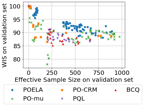
Figure 3: Trade-off between ESS and value estimates.

E.4 Eligible actions visualization for high/mid/low-SOFA patients

In this section, we explore the learned policies for patients with high logged SOFA scores (measuring organ failure) in the test dataset. Figure 4 illustrates the number of actions taken by different policies and the clinicians. POELA mainly takes treatments similar to the clinician’s but more concentrated on high-vasopressors treatments, while PO-CRM and value-based methods take treatments different from the logged clinician decisions, suggesting these policies may be overfitting to avoid contexts with high SOFA. However, some patients arrive with high SOFA scores and a policy must have suitable treatments to support such individuals, which our method appears to ensure. For completeness, we also show the visualization of mid-SOFA ($5-15$) and low-SOFA ($<5$) patient contexts in Figures 4 and 4.

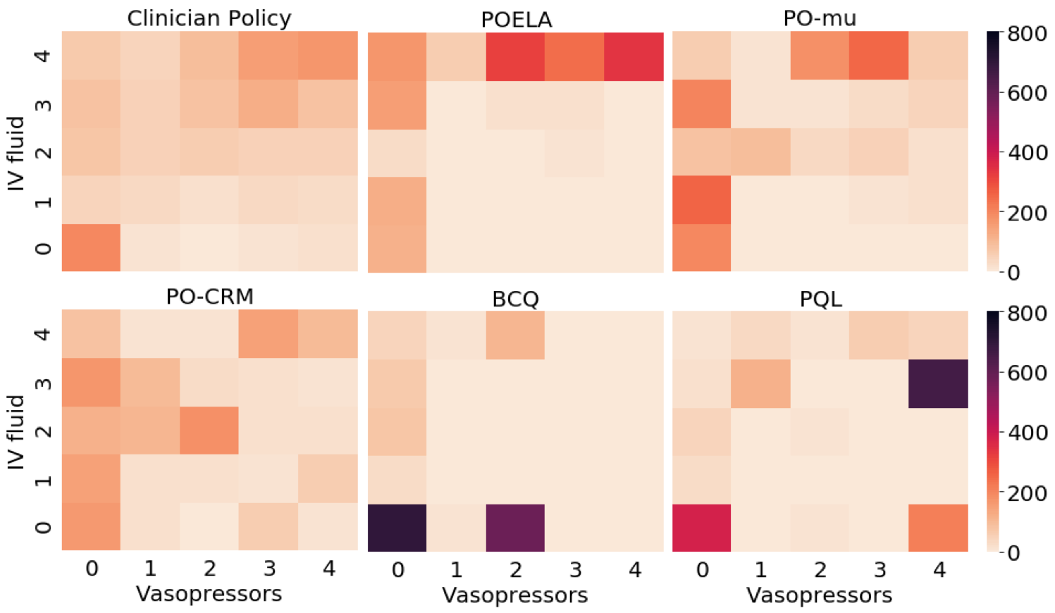
(a) Action counts in high-SOFA contexts

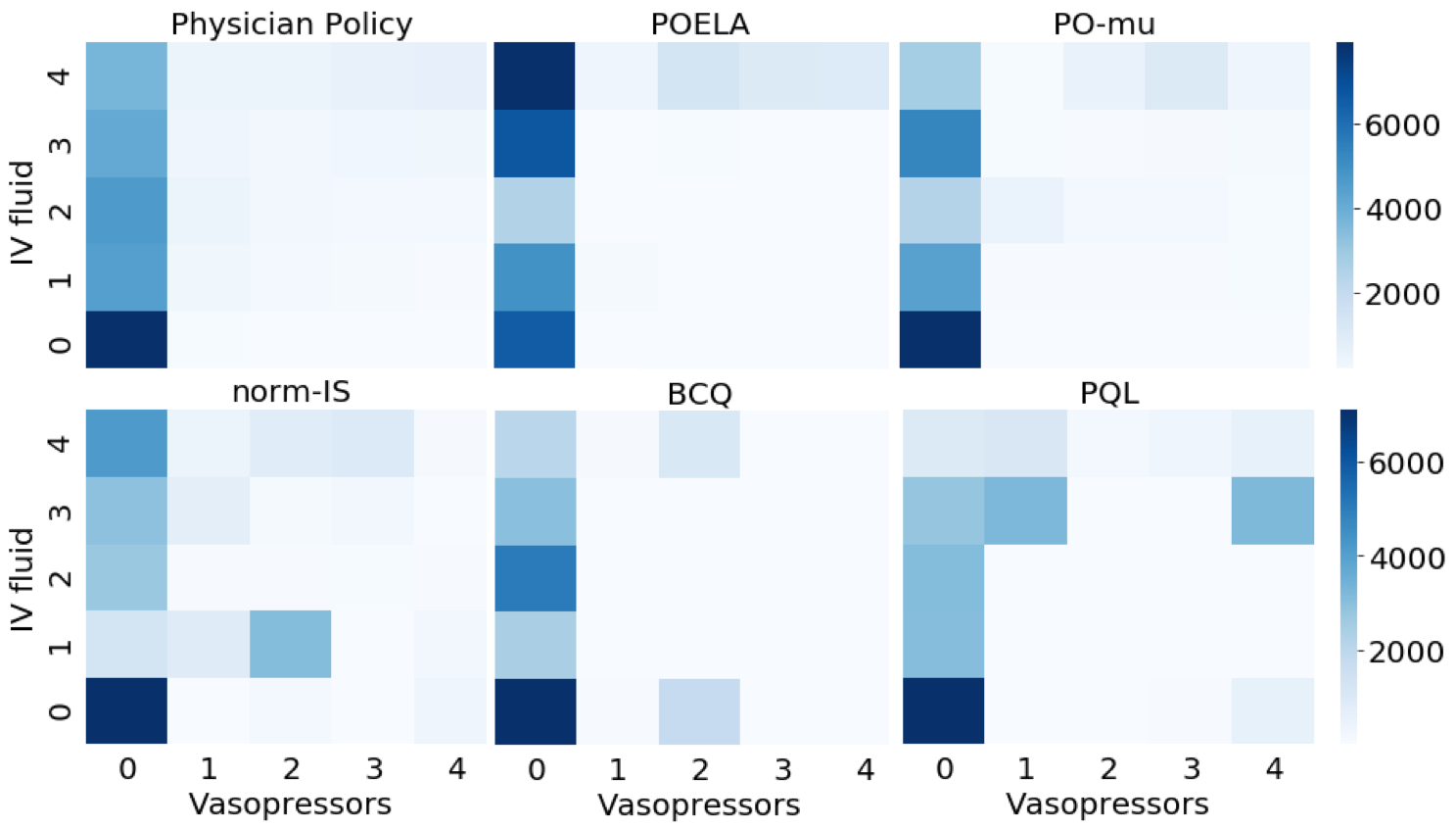
(b) Action counts in mid-SOFA contexts

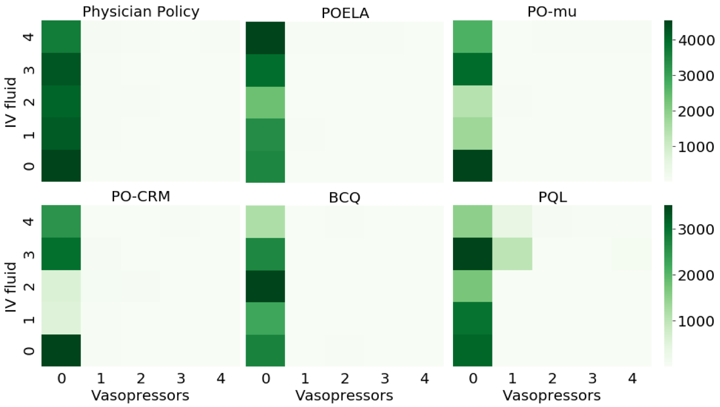
(c) Action counts in low-SOFA contexts

Figure 4: (a): Action counts heatmap in high-SOFA contexts of the policy learned from different algorithms. (b): Action counts heatmap in mid-SOFA contexts of the policy learned from different algorithms. (c): Action counts heatmap in low-SOFA contexts of the policy learned from different algorithms.

Appendix F Additional experiments: OpenAI Gym environment CartPole

In this experiment, we collect a dataset by training DQN [Mnih et al., 2013] on the task and saving trajectories of horizon 200 steps at regular checkpoints during the training. The dataset is composed of a mixture of sub-optimal and expert data totalling 20000 transitions. For the non-Markov modification, we keep the Cart Position, Cart Velocity and Pole Angle observations but remove the Pole Angular Velocity element. In Table 19, we report the hyperparameter used in the experiments.

Hyperparameters	used in algorithms	values
$\delta$	POELA	$0.0001,0.0005,0.001,0.005,0.01$
$\hat{\mu}$ threshold	PO-$\mu$	0.05, 0.1, 0.15, 0.2
CRM Var coefficient	POELA, PO-CRM	$0,0.1,1,10$
BCQ threshold	BCQ, PQL	$0.0,0.05,0.1,0.2,0.5$
$M$ in $\hat{v}_{\text{SNTIS}}$	All	$1000$
Max training steps	POELA, PO-CRM, PO-$\mu$	500
	BCQ, PQL	1000
Number of checkpoints	All	50
Batch size	BCQ, PQL	64

Table 19: Hyperparameters in the CartPole experiment.

F.1 Standard evaluation procedure: use policy at the end of training

Method	POELA	PO-$\hat{\mu}$	PO-CRM	BCQ	PQL	Behavior policy
Test SNTIS	88.29 (86.62)	78.79	72.63	21.28	23.61	41.41
$95\%$ BCa UB	89.70 (89.81)	83.87	76.77	24.63	27.14	45.04
$95\%$ BCa LB	85.93 (85.57)	69.64	68.15	16.22	20.36	38.16
Test ESS	43.32 (40.78)	30.51	30.13	30.11	30.08	248

Table 20: CartPole dataset. Test evaluation, $(0.05,0.95)$ BCa bootstrap interval, and ESS. The value of POELA without a CRM variance penalty is shown in parentheses.

Method	POELA	PO-$\hat{\mu}$	PO-CRM	BCQ	PQL	Behavior policy
Test SNTIS	76.18 (72.21)	68.39	67.14	12.13	5.46	41.41
$95\%$ BCa UB	89.27 (88.32)	80.22	83.72	12.89	6.63	45.04
$95\%$ BCa LB	68.97 (67.49)	57.13	57.78	9.17	5.02	38.16
Test ESS	36.41 (34.72)	34.56	31.87	31.22	30.07	248

Table 21: Non-MDP CartPole dataset. Test evaluation, $(0.05,0.95)$ BCa bootstrap interval, and ESS. The value of POELA without a CRM variance penalty is shown in parentheses.

F.2 Alternative selection procedure: checkpoint best intermittent policies

Method	POELA	PO-$\hat{\mu}$	PO-CRM	BCQ	PQL	Behavior policy
Test SNTIS	88.43 (87.56)	76.01	82.25	17.74	17.83	41.41
$95\%$ BCa UB	90.46 (90.72)	82.87	86.18	21.80	21.84	45.04
$95\%$ BCa LB	85.48 (84.63)	66.21	74.30	12.84	13.26	38.16
Test ESS	43.32 (39.66)	31.04	30.87	30.29	30.18	248

Table 22: CartPole dataset. Test evaluation, $(0.05,0.95)$ BCa bootstrap interval, and ESS. The value of POELA without a CRM variance penalty is shown in parentheses. Procedure: best intermittent policy checkpoints.

Method	POELA	PO-$\hat{\mu}$	PO-CRM	BCQ	PQL	Behavior policy
Test SNTIS	75.76 (75.70)	68.66	66.34	11.73	5.70	41.41
$95\%$ BCa UB	92.35 (89.16)	79.56	82.46	12.49	6.71	45.04
$95\%$ BCa LB	68.34 (66.08)	55.49	57.50	7.98	5.08	38.16
Test ESS	37.72 (35.27)	35.15	36.02	30.12	31.77	248

Table 23: Non-MDP CartPole dataset. Test evaluation, $(0.05,0.95)$ BCa bootstrap interval, and ESS. The value of POELA without a CRM variance penalty is shown in parentheses. Procedure: best intermittent policy checkpoints.

Appendix G Additional experiments: D4RL

Although our primary focus is on application areas where the Markov assumption may not be correct or unverifiable, we also compare to an additional standard benchmark, namely D4RL.

An adaptation of the POELA algorithm is necessary to work with continuous action spaces. Practically, instead of using the eligible action set $A_{h}$, for each data sample, we pre-compute a set of similar actions and use the distance to the closest state $x_{h}$ associated with the most similar action distributions in the dataset as a smooth penalty in Line 5 of Algorithm 1.

For each dataset quality (random, medium, and expert) and task (Hopper and Walker2D), we report the performances scaled from 0 to 100 (0 corresponds to the average returns of a random policy and 100 that of an expert policy) following the experimental protocol for D4RL with 200 episodes in each dataset. We compare with state-of-the-art methods in this dataset. The results are reported in Table 24.

Dataset	POELA	BCQ	CQL	Behavior policy
Hopper-random	10.5	10.5	10.8	9.8
Hopper-medium	43.7	42.9	41.4	29.0
Hopper-expert	58.9	59.7	52.6	43.6
Walker2D-random	6.1	4.6	5.4	1.6
Walker2D-medium	33.8	31.1	49.6	6.6
Walker2D-expert	32.2	32.8	54.7	50.2

Table 24: Additional experiments on 6 D4RL datasets.

The results in Table 24 suggest that POELA performs similarly to two other state-of-the-art methods in this setting, even though POELA does not make Markov assumptions, which are made and leveraged in BCQ and CQL.