Ranking Theoretical Supernovae Explosion Models from Observations of the Intracluster Gas

Abstract

The intracluster medium (ICM) is a reservoir of heavy elements synthesized by different supernovae (SNe) types over cosmic history. Different enrichment mechanisms contribute a different relative metal production, predominantly caused by different SNe Type dominance. Using spatially resolved X-ray spectroscopy, one can probe the contribution of each metal enrichment mechanism. However, a large variety of physically feasible supernova explosion models make the analysis of the ICM enrichment history more uncertain. This paper presents a non-parametric PDF analysis to rank different theoretical SNe yields models by comparing their performance against observations. Specifically, we apply this new methodology to rank 7192 combinations of core-collapse SN and Type Ia SN models using 8 abundance ratios from Suzaku observations of 18 galaxy systems (clusters and groups) to test their predictions. This novel technique can compare many SN models and maximize spectral information extraction, considering all the individual measurable abundance ratios and their uncertainties. We find that Type II Supernova with nonzero initial metallicity progenitors in general performed better than Pair-Instability SN and Hypernova models and that 3D SNIa models (with the WD progenitor central density of $2.9\times 10^{9}\mathrm{g\,cm^{-3}}$) performed best among all tested SN model pairs.

1 Introduction

The discovery of the non-pristine hot intracluster medium (ICM) over 40 years ago (Mitchell et al., 1976; Serlemitsos et al., 1977) established a link between stellar and supernova (SN) nucleosynthesis products in galaxies and metals (i.e., heavy elements) in the ICM (or in the intragroup medium, IGrM). Supernovae events play a dominant role in synthesizing and ejecting heavy elements and can offer clues to processes involved in the ICM chemical enrichment. Core collapse supernovae (SNcc) produce significant amounts of oxygen (O), neon (Ne), magnesium (Mg), silicon (Si), sulfur (S), argon (Ar), and calcium (Ca), as compared to iron (Fe) and its neighboring elements, such as nickel (Ni), mainly produced, instead, primarily by Type Ia supernovae (SNIa). Despite the general picture of the metal production, there are still uncertainties about the amount of synthesized metals (yields) by the different SNe types, related to their explosion mechanisms and the nature of their progenitors.

Type Ia supernovae are generally associated to thermonuclear explosions of carbon and oxygen white dwarfs (C+O WD) in binary star systems. However, the nature of the companion star is still uncertain (see reviews by Maeda & Terada 2016, Seitenzahl & Townsley 2017, and Livio & Mazzali 2018). The accreted material can come from a non-degenerate companion star (single degenerate scenario, Whelan & Iben Jr, 1973) or another white dwarf (WD) (double degenerate scenario, Iben & Tutukov, 1984; Webbink, 1984). The physics of the propagation burning front is also under debate (Hillebrandt & Niemeyer, 2000). Central detonation models of near-Chandrasekhar mass ($M_{Ch}\sim 1.4M_{\odot}$) WDs (Arnett, 1969; Hansen & Wheeler, 1969) produce insufficient amounts of intermediate mass elements (IMEs), such as S and Si, needed to explain the observed SNIa spectra. Deflagration models allow the WD to expand to lower density conditions suitable to the synthesis of IMEs but still fall short in reproducing their observed spectra (Fink et al., 2014). Delayed-detonation models such as deflagration-to-detonation transition (Khokhlov, 1991), gravitationally confined detonations (Plewa et al., 2004; Jordan et al., 2008), and pulsating reverse detonations (Bravo et al., 2009), arise as a reasonable option to overcome the nucleosynthetic deficiencies to explain normal SNIa. Different mechanisms can also lead to SNIa in the sub-$M_{Ch}$ scenario, involving violent mergers of two C+O WDs (e.g. Pakmor et al., 2010, 2012), direct collisions of two C+O WDs with or without He-shells (e.g. Papish & Perets, 2016), double-detonations of WD with He shells (e.g. Leung & Nomoto, 2020a), and dynamically driven double-degenerate double-detonations (e.g. Shen et al., 2018).

Core collapse supernovae (SNcc) are related to the death of massive stars ($\gtrsim 10M_{\odot}-140M_{\odot}$ see Nomoto et al., 2013, for a review). Their nucleosynthetic products depend on the initial mass and metallicity of the progenitor stars, the mass cut separating the final core mass and the remnant ejected mass, and the final kinetic energy (e.g. Chieffi & Limongi, 2004; Nomoto et al., 2013). Moreover, to determine the yields in populations of massive stars, the considered initial mass function (IMF) is also an additional uncertain factor. As a result, all these uncertainties lead to numerous theoretical explosion models for both SNIa and SNcc present in the literature, where competing models often exhibit discrepant heavy element abundance patterns.

The metals in the ICM can be seen as a reservoir of ejecta from SNIa and SNcc explosions. There are many processes involved in producing the chemical enrichment of the ICM, the relative importance of each of them is still under debate (for a review see e.g. Schindler & Diaferio, 2008; Mernier et al., 2018a). They might include SN II powered galactic winds (Larson & Dinerstein, 1975), ram-pressure stripping of gas from galaxies (Gunn & Gott, 1972) after cluster formation, or ICM metal enrichment could have happened in the environment before cluster’s virialization (pre-enrichment) (e.g. Biffi et al., 2018). The importance of each of these mechanisms can be assessed through comparison to SNe yield models if these models are well constrained. However, as mentioned above, there are still significant uncertainties about the predicted yields for different SN Types, and one can, in principle, invert the problem and use bona fide abundances observed in the ICM to differentiate among various SNe explosion models. This iteration is justified because the ICM is generally optically thin to X-rays and close to collisional ionization equilibrium (see reviews by Böhringer & Werner 2010 and Mernier et al. 2018a), making abundance measurements clean and easy to derive.

Abundance measurements from X-ray spectroscopy have proven to be a powerful tool to constrain theoretical supernova yield models (Dupke & White, 2000; Finoguenov et al., 2002; Sato et al., 2007; de Plaa et al., 2007; Bulbul et al., 2012; Mernier et al., 2016; Simionescu et al., 2019). This work applies a new technique to improve the power of elemental abundance ratios measured in a selected cluster sample to rank different theoretical SNe explosion models. The sample is composed of 18 carefully selected nearby galaxy systems, such that (i) the internal and external regions can be cleanly separated and (ii) the particle background is low enough, so we do not need to worry about particle background modeling, which would introduce additional uncertainties. Thanks to the very low particle background combined with an excellent spectral resolution, the X-ray Imaging Spectrometer (XIS) on-board of Suzaku is the most suitable for measuring individual abundances accurately. Our technique identifies the level of incompatibility with the observations between an extensive set of SNIa and SNcc predicted yield models by individually assessing eight abundance ratios (O/Fe, Ne/Fe, Mg/Fe, Si/Fe, S/Fe, Ar/Fe, Ca/Fe, and Ni/Fe) in a non-parametric analysis based on the Kolmogorov-Smirnov test (KS test, hereafter). We compare them to those predicted by 7192 different combinations SNIa–SNcc pairs among 263 theoretical supernova yield models found in the literature.

This paper is organized as follows. In Section 2, we describe the data preparation and reduction, as well as the spectra modeling of the sample. The comparison between the predicted yields from SN models and the measured ratio abundances from observations is detailed in Section 3. We then implement our methodology to quantify the incompatibility of the theoretical yields with the abundance ratio measurements in Section 4 over 263 theoretical supernovae yield models, whose main properties are quickly described in Section 5. Our main results are presented in Section 6 and we summarize our main conclusions in Section 7. We assume cosmological parameters being $H_{0}=67.8$ km s^-1 Mpc^-1, $\Omega_{m}$=0.308, and $\Omega_{\Lambda}$=0.692 (Planck Collaboration et al., 2016). Error bars of abundance ratios are given at 68% significance level. We adopt the metal solar abundance model by Anders & Grevesse (1989, hereafter ANGR).

2 Data Preparation

Table 1: Observations of groups and clusters of galaxies.

Cluster/Group name	RA	DEC	Redshifta	Cool-core radius	Obs ID	Exposure time	PI Name
	(hh:mm:ss)	(dd:mm:ss)		(kpc)		(ks)
NGC 5846	15 06 29.62	+01 36 09.0	0.0060	$\lesssim 20$	803042010	155,9	M. Loewenstein
NGC 4472	12 29 46.58	+08 00 18.0	0.0044	$\lesssim 10$	801064010	121,0	M. Loewenstein
HCG62	12 53 05.76	-09 12 07.9	0.0147	$\lesssim 30$	800013020	114,8	N. Ota
Ophiuchus	17 12 26.23	-23 22 44.4	0.0280	$\lesssim 40$	802046010	100,5	A. Furuzawa
NGC 1550	04 19 47.71	+02 24 37.8	0.012	$\lesssim 25$	803017010	83,3	K. Sato
Abell 3581	14 07 37.99	-27 01 11.6	0.0226	$<100$	807026010	80,4	K. Sato
NGC 507	01 23 38.52	+33 15 35.3	0.01902	$\lesssim 40$	801017010	79,5	K. Sato
Abell 426	03 19 49.30	+41 30 14.0	0.0179	$\lesssim 100$	800010010	50,4	A. Fabian
Abell 496	04 33 39.50	-13 16 44.8	0.0329	$<90$	803073010	44,3	R. Dupke
Abell 3571	13 47 26.98	-32 51 08.6	0.0391	$\lesssim 100$	808094010	38,3	R. Dupke
Abell 262	01 52 46.13	+36 09 32.8	0.01641	$<40$	802001010	37,2	K. Matsushita
NGC 2300	07 31 15.79	+85 41 47.4	0.0070	$<20$	804030010	37,1	K. Matsushita
Abell 3526	12 48 48.29	-41 18 47.5	0.0104	$<50$	800014010	36,5	Y. Fukazawa
MKW4	12 04 32.88	+01 54 50.8	0.01975	$<25$	808066010	34,6	Y. Su
NGC 5044	13 15 24.10	-16 23 23.6	0.0082	$<40$	801046010	19,7	K. Matsushita
AWM7	02 54 31.44	+41 35 35.9	0.0172	$<30$	801035010	19,0	T. Ohashi
NGC 6338	17 15 15.10	+57 25 14.9	0.02816	$<70$	809099010	15,5	L. Lovisari
UGC 3957	07 40 58.39	+55 25 44.4	0.0340	$\lesssim 110$	801072010	10,8	C. Scharf

Note. — The first three columns show the target names and their equatorial coordinates. The ^aFourth column (z) shows the corresponding redshifts taken from NASA/IPAC Extragalactic Database (2019) (NED) to perform spectral fittings (see Section 2.2). The fifth column (Inner radius) indicates the radius that delimits the inner regions of each group/cluster. The last three columns (ObsID, Exposure time, and PI Name) are related to its observation identification number, exposure time, and the name of the principal investigator on the proposal, respectively.

Our analysis is based on 18 nearby ($z\leq 0.0391$) groups and clusters of galaxies observed with the X-ray Imaging Spectrometer observations on-board the Suzaku satellite. Their properties are presented in Table 1. Downloaded observations from the HEASARC website were processed as follows. We selected the observations with the longest exposure time available for each object in the sample. We calibrated and screened 4 XIS chips (XIS0, 1, 2 & 3), when available, via aepipeline tool. We applied standard criteria using HEAsoft v6.21. Editing mode data 5x5 were converted and combined to 3x3 event files with XSELECT v2.4d. We extracted three regions - inner, outer and total - for each object. The inner region is where one would expect higher contamination of metals from SNIa in the cool-core galaxy groups and clusters (see Section 2.1). Spectra channels were grouped with $\geq 10$ counts per channel. Redistribution matrices and ancillary response files were generated using xisrmfgen and xissimarfgen, respectively. Observations of the North Ecliptic Pole were used as background observations. We applied the same screening criteria described above for the background observation (ID 100018010).

2.1 Regions selection

We used three regions for each cluster, an inner region encompassing (nearly) the entire cool-core, an outer region built to avoid cool-core contamination, and a full field-of-view (FoV) region. We selected cool-core clusters with central Fe abundance gradients. The innermost regions of cool-core clusters have particular characteristics. Fe abundance and surface brightness peak at the center, while temperature falls typically to $\sim 2-3$ times lower than the outskirt values. Non-cool-core clusters lack the surface brightness peak and central temperature drop (e.g. De Grandi & Molendi, 2001). We exploit the central Fe excess adopting inner region sizes that maximize the Fe abundance excess, encompassing the cool-core domain. The Fe abundance peak in the center of the cool-core galaxy systems may be a result of an extensive period of enrichment by SNIa explosions deposited in or created by the brightest cluster galaxy (De Grandi et al., 2004; Böhringer et al., 2004). While early studies suggested a relatively higher contribution of the Fe mass fraction from SNIa ejecta in the central regions of cool core clusters compared to the outer regions (e.g. Dupke & White, 2000; Finoguenov et al., 2000), this was not shown to be ubiquitous and also not systematically found across all measured ratios (e.g. de Plaa et al., 2006; Simionescu et al., 2009; Böhringer & Werner, 2010; Mernier et al., 2017, and references therein). However, the presence of such a radial gradient of SNIa/SNcc Fe mass fraction could increase the ranking power of SN explosion model pairs by our method by analyzing the central and outer regions separately. If the gradient is not present, the separation of inner/outer regions would smooth out the ranking ability of specific abundance ratios due to the increased errors associated with having fewer counts. But even so, it should provide similar ranking results. For this reason, we choose to measure the abundances separately from the innermost and outermost regions to potentially maximize the range of variation of SNIa/SNcc yield mass fraction, improving the ranking power of the method.

The redshift spanned by the sample is based on both the point spread function (PSF) and the field-of-view of Suzaku. The inner regions are circles, with radii varying from $1\arcmin$ to $4\arcmin$. The variation of the inner region size is chosen to take into account the cool-core radius and the minimization of Suzaku PSF contamination. We assessed the cool-core radius from the ACCEPT project (Cavagnolo et al., 2009), except for Abell 3571 (Dupke & White, 2000; Eckert et al., 2011), the NGC 6338, NGC 2300, (Rasmussen & Ponman, 2007), NGC 4472 (Kraft et al., 2010), NGC 1550 (Kolokythas et al., 2020), and UGC 3957 (Thölken et al., 2016) groups. Outer regions are annuli with a radius $\geq 5\arcmin$ to reduce contamination from the cool-core vicinity. Full FoV regions (i.e., total regions) have $8\arcmin$ of radius.

2.2 Spectral Models

We fit each cluster/group to the optically thin thermal plasma cluster/group emission vapec model. Elemental abundances of O, Ne, Mg, Si, S, Ar, Ca, Fe, and Ni were free to vary and temperature and normalization. Cluster emission is expected to be absorbed by foreground Galactic gas, characterized by wabs model (Morrison & McCammon, 1983). We then adopted a fixed Galactic hydrogen column of $N_{H}$ collected from the HEASARC $N_{H}$ tool. We included a power-law component to model active galaxy nuclei (AGN) emission when needed, based on visual inspection of archival Chandra observations (only for inner and total regions). We fixed the power-law index at 1.9, as found by the high-resolution Hitomi analysis of NGC 1275 (Hitomi Collaboration et al., 2017), but its normalization is a free parameter. The energy band range of spectral fits was limited to 0.5–8.0 keV. We fitted individual spectra for each cluster/group, region, and XIS instrument. For instance, the inner region of the Centaurus Cluster has four abundances of Si (from XIS0, 1, 2 & 3), and we calculate their error-weighted average to obtain a final value of Si abundance. We repeated this procedure for each object, instrument, region, and elemental abundance measurement. We report the final error-weighted average of temperature and chemical abundances for each region in Table 2. Then, we determined and compared these final abundance ratios of O/Fe, Ne/Fe, Mg/Fe, Si/Fe, S/Fe, Ar/Fe, Ca/Fe, and Ni/Fe with those predicted by SN explosion models. We performed the spectral fittings with XSPEC v12.9.1 (Arnaud, 1996) and AtomDB v3.0.7 assuming a $\chi^{2}$ statistic.

3 Supernova Model Yields and Observed ICM comparison

Metals in the ICM have origin in different stellar sources. We assume that the heavy elements observed in the ICM/IGrM originate ultimately from ejected material of two SN Types, SNIa and SNcc, the latter representing all core-collapse SNe. The chemical enrichment of the ICM can then be quantified by the linear combination of each SN type. The observed number of atoms in the ICM, $N(\mathrm{E})$, of a certain element E, is expressed as

$$\underbrace{N(\mathrm{E})}_{\text{observed in the ICM}}=\underbrace{n_{i}N_{i}^{\text{Ia}}(\mathrm{E})+n_{j}N_{j}^{\text{cc}}(\mathrm{E})}_{\text{predicted by SN models}},$$ (1)

where $N_{i}^{\text{Ia}}(\mathrm{E})$ and $N_{j}^{\text{cc}}(\mathrm{E})$ are the number of atoms predicted by the SNIa model $i$ and SNcc model $j$, respectively, where $i=\{1,2,...\,,232\}$ refers to the 232 SNIa models considered, and $j=\{1,2,...\,,31\}$, indexes the 31 SNcc models. The numerical abundances $A_{i}^{\text{Ia}}(\mathrm{E})$ and $A_{j}^{\text{cc}}(\mathrm{E})$ are the number of atoms of a given element E divided by the number of atoms of Hydrogen (H), normalized to the same ratio for the solar value, produced by the SNIa and SNcc models $i$ and $j$, respectively. The coefficients $n_{i}$ and $n_{j}$ are the number of SNIa and SNcc that enriched the ICM calculated adopting models $i$ and $j$, respectively. The argument E represents the chemical element considered, where E={O, Ne, Mg, Si, S, Ar, Ca, Fe, Ni}.

To calculate the predicted abundance $A_{i}^{\text{Ia}}$ (relative to H) of a given element E, defined as

$$A_{i}^{\text{Ia}}=A_{i}^{\text{Ia}}(\mathrm{E})\equiv\frac{[N_{i}^{\text{Ia}}(\mathrm{E})/N(\mathrm{H})]}{[N(\mathrm{E})/N(\mathrm{H})]_{\odot}},\\$$ (2)

we derive the number of atoms, $N_{i}^{\text{Ia}}$, of a given element E via the relation below:

$$N_{i}^{\text{Ia}}=N_{i}^{\text{Ia}}(\mathrm{E})=\frac{Y_{i}^{\text{Ia}}(\mathrm{E})}{\mu(\mathrm{E})},$$ (3)

where $Y_{i}^{\text{Ia}}(\mathrm{E})$ is the mass yield of the element E (simulated) by the SNIa model $i$ and $\mu(\mathrm{E})$ is the atomic mass of the element E. $N(\mathrm{E})$ and $N(\mathrm{H})$ are the number of atoms of the elements E and Hydrogen, respectively, where $[N(\mathrm{E})/N(\mathrm{H})]_{\odot}$ represents that ratio for the sun, i.e., solar abundance (in this work we use solar abundances of ANGR). The results obtained in this work are not affected by the choice of the solar abundance table.

Our collection of SNe models encompasses the current models with published yields, $Y_{i}^{\text{Ia}}$ and $Y_{j}^{\text{cc}}$, of a given element E and are listed in Tables 3 and 4 in the Appendix E. While $Y_{i}^{\text{Ia}}$ are taken directly from the yield tables, the SNcc yields are provided only for discrete progenitor masses (m), with a given initial progenitor metallicity $Z_{\rm init}$, $Y_{j}^{\text{cc}}(m,\mathrm{E},Z_{\rm init})$. We then used a Salpeter IMF (Salpeter, 1955) with slope $\alpha=-2.35$ to weigh these discrete yields within the mass limits simulated ($m_{j,\text{low}}$ to $m_{j,\text{up}}$) for a common $Z_{\rm init}$. The total average yield mass, $\overline{Y}_{j}^{\text{cc}}(\mathrm{E},Z_{\rm init})$, of a given element E weighted over the Salpeter IMF within $m_{j,low}$ and $m_{j,up}$ at a given initial metallicity of the progenitor star, $Z_{\rm init}$, is expressed as

$$\overline{Y}_{j}^{\text{cc}}=\overline{Y}_{j}^{\text{cc}}(\mathrm{E},Z_{\rm init})=\frac{\displaystyle\int_{m_{j,\text{low}}}^{m_{j,\text{up}}}Y_{j}^{\text{cc}}(m,\mathrm{E},Z_{\rm init})\ m^{\alpha}\,dm}{\displaystyle\int_{m_{j,\text{low}}}^{m_{j,\text{up}}}m^{\alpha}\ dm}\,,$$ (4)

where $Y_{j}^{\text{cc}}(m,\mathrm{E},Z_{\rm init})$ is the yield predicted by SNcc model $j$ of a given element E produced by an initial progenitor stellar mass $m$ with an initial metallicity $Z_{\rm init}$.

The individual elemental abundance ratio of a given element E to that of Fe, $R(\mathrm{E})$, using Equations (1)–(3), can be written as:

$$\textstyle R(\mathrm{E})=f_{i}\,R_{i}^{\text{Ia}}(\mathrm{E})+f_{j}\,R_{j}^{\text{cc}}(\mathrm{E})\,,$$ (5)

where

$$R_{i}^{\text{Ia}}=R_{i}^{\text{Ia}}(\mathrm{E})\equiv\frac{A_{i}^{\text{Ia}}(\mathrm{E})}{A_{i}^{\text{Ia}}(\text{Fe})}=\bigg{(}\frac{N_{i}^{\text{Ia}}(\mathrm{E})}{N_{i}^{\text{Ia}}(\text{Fe})}\bigg{)}\bigg{/}\bigg{(}\frac{N(\mathrm{E})}{N(\text{Fe})}\bigg{)}_{\odot}\,.\\$$ (6)

Here, $R_{i}^{\text{Ia}}(\mathrm{E})$ and $R_{j}^{\text{cc}}(\mathrm{E})$ are the abundance ratios of element E predicted by the SNIa model $i$ and SNcc model $j$, respectively. The $f_{i}$ and $f_{j}$ represent the iron mass fractions that result from enriching the ICM using the SNIa model $i$ and SNcc model $j$. An analogous expression of Equation (6) can be easily obtained for SNcc using the same formalism denoted by the index $j$ in Equations (2), (3) and (6).

The iron mass fraction of the respective SNIa from model $i$ and SNcc from model $j$ that enriches the ICM, $f_{i}$ and $f_{j}$, are then expressed as

$$f_{i}=\frac{Y_{i}^{\text{Ia}}(\mathrm{Fe})\overline{Y}_{j}^{\text{cc}}(\mathrm{Fe})-Y_{i}^{\text{Ia}}(\mathrm{Fe})\overline{Y}_{j}^{\text{cc}}(\mathrm{E})\frac{A(\mathrm{Fe})}{A(\mathrm{E})}\frac{\mu(\mathrm{Fe})}{\mu(\mathrm{E})}\big{(}\frac{N(\mathrm{E})}{N(\text{Fe})}\big{)}_{\odot}}{\frac{A(\mathrm{Fe})}{A(\mathrm{E})}\frac{\mu(\mathrm{Fe})}{\mu(\mathrm{E})}\big{(}\frac{N(\mathrm{E})}{N(\text{Fe})}\big{)}_{\odot}\left[Y_{i}^{\text{Ia}}(\mathrm{E})\overline{Y}_{j}^{\text{cc}}(\mathrm{Fe})-Y_{i}^{\text{Ia}}(\mathrm{Fe})\overline{Y}_{j}^{\text{cc}}(\mathrm{E})\right]}\,,$$ (7)

where, by definition

$$f_{i}+f_{j}\equiv 1\,.$$ (8)

The numerical abundance measured in the ICM of a given element E and Fe are represented by $A(\mathrm{E})$ and $A(\mathrm{Fe})$, respectively. The number of SNIa per SNcc enriching the ICM, $\eta\equiv n_{i}/n_{j}$, in terms of fundamental parameters can be derived as

$$\eta\equiv\frac{n_{i}}{n_{j}}=\frac{\overline{Y}_{j}^{\text{cc}}(\mathrm{E})\frac{M(\mathrm{Fe})}{M(\mathrm{E})}-\overline{Y}_{j}^{\text{cc}}(\mathrm{Fe})}{Y_{i}^{\text{Ia}}(\mathrm{Fe})-Y_{i}^{\text{Ia}}(\mathrm{E})\frac{M(\mathrm{Fe})}{M(\mathrm{E})}}\,,$$ (9)

where $M(\mathrm{Fe})$ and $M(\mathrm{E})$ are the total gas mass in the ICM originally from Fe and element E, respectively.

In Section 4, we compare these theoretical abundance ratios from a SNIa and SNcc models ($R_{i}^{\text{Ia}}(\mathrm{E})$ and $R_{j}^{\text{cc}}(\mathrm{E})$, respectively) to the observed abundance ratio distribution of a given element E.

4 Evaluation of Supernovae Explosion Models

The Kolmogorov-Smirnov test is a non-parametric statistical test that compares the cumulative distribution function (CDF) of two samples under the null hypothesis that these two samples are drawn from the same distribution (see Ivezić et al., 2014, for details). $D_{i,j}(\mathrm{E})$ is the metric that measures the maximum distance between two cumulative distribution functions (CDF) built for a given element E and drawn from the observations, and specific pair $(i,j)$ of supernova models, defined as

$$D_{i,j}(\mathrm{E})=\mathrm{max}\left|\mathrm{eCDF}(R(\mathrm{E}))-\mathrm{tCDF}(R_{i}^{\text{Ia}}(\mathrm{E}),R_{j}^{\text{cc}}(\mathrm{E}))|\right.$$ (10)

These two CDFs are built as follows. Firstly, we build the empirical cumulative distribution function (eCDF) from the measured abundance ratios of the ICM of a given element E ($\mathrm{eCDF}(R(\mathrm{E}))$, see Section 4.1). Secondly, the theoretical cumulative distribution function (tCDF) is associated with the theoretical abundance ratios of a pair of SN models, $R_{i}^{\text{Ia}}(\mathrm{E})$ and $R_{j}^{\text{cc}}(\mathrm{E})$, composed by a certain SNIa model $i$ and a SNcc model $j$ ($\mathrm{tCDF}(R_{i}^{\text{Ia}}(\mathrm{E}),R_{j}^{\text{cc}}(\mathrm{E}))$, see Section 4.2). This tCDF is built using those ratios as the limits of the probability distribution function (PDF) and the assumption that, in between these limits, each value has the same probability, i.e., a flat PDF.

We choose a pre-established significance level $\alpha=0.05$ as the threshold to reject the null hypothesis. Hence, when a p-value is lower than the threshold, we can conclude that the two distributions are too dissimilar to be drawn from the same distribution at a 95% significance level and, thus, we reject the null hypothesis. We implement the two-sample Kolmogorov-Smirnov test adapting the scipy.stats.kstest routine of the SciPy-Python library (Virtanen et al., 2020) to compute the KS statistics $D_{i,j}(\mathrm{E})$ and the respective p-values.

4.1 Empirical Cumulative Distribution Function (eCDF)

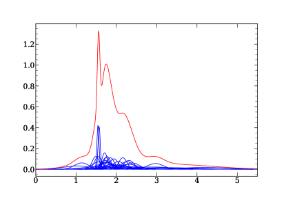
Figure 1: Probability Distribution Function of Si/Fe abundance ratio measurements of inner and outer regions. Blue lines indicate the Si/Fe measurement for each object in our sample, represented by normal distributions whose mean is the nominal Si/Fe value and the standard deviation is the respective error. The red line is the final sum of each normal distribution in our sample. We also present the PDFs for others abundance ratios in the Appendix A in Figure 12.

We built the empirical CDF considering the nominal values of the observed abundance ratios and their associated errors. For the sake of illustration, we describe the procedure using the Si/Fe abundance ratio to evaluate a pair of SN models as an example. We assumed that each Si/Fe measurement could be modeled as a normal distribution centered in the nominal value of the abundance ratio with a standard deviation given by its error. Figure 1 shows the normal distributions of Si/Fe ratios, $R(\mathrm{E})$, for each galaxy cluster and group (blue lines) in our sample. The total probability distribution function of Si/Fe (red line) is obtained by summing and normalizing the individual normal distributions. We can easily calculate the corresponding eCDF of Si/Fe (green line, Figure 2) using the total probability distribution. This procedure is repeated for each one of the eight abundance ratios considered in this work. The PDFs for others abundance ratios are presented in the Appendix A in Figure 12.

4.2 Theoretical Cumulative Distribution Function (tCDF)

The observed abundance ratios can be expressed as a (linear) combination of yields produced by both SN types (see Section 3). For this reason, we build a single theoretical CDF per pair of SNe models, i.e., composed of one SNIa and one SNcc model.

To illustrate the procedure, as an example, we chose the yields of the SNIa WDD1 delayed-detonation model of Iwamoto et al. (1999) (Iw99_WDD1 model) and the Type II supernova solar metallicity model of (Nomoto et al., 2013) (No13_SNII_Z2E-2 model), respectively. We then employ the Si/Fe ratio predictions from the Iw99_WDD1 model and No13_SNII_Z2E-2 model, which are $R(\texttt{Si})_{\text{\tiny WDD1}}^{\text{Ia}}=1.067$ and $R(\texttt{Si})_{\text{\tiny SNIIZ2E-2}}^{\text{cc}}=4.43$, respectively (for definition, see Eq. (6)).

We built the tCDF as a piecewise function defined as follows. For a 100% SNIa enrichment of the ICM (and therefore no contribution by SNcc), the abundance ratio would correspond to $R(\texttt{Si})\sim 1.067$, as predicted by the Iw99_WDD1 model solely. In the opposite extreme case, where all the enrichment comes from SNcc, $R(\texttt{Si})\sim 4.43$, as estimated by the No13_SNII_Z2E-2 model. This implies that: (i) any intermediate measurement $1.067<R(\texttt{Si})<4.43$ must come from a linear combination of both SN types, and (ii) this pair of SN models can only explain the observed abundance ratio between $1.067$ and $4.43$, so that the probability of measuring a $R(\texttt{Si})$ lower than $1.067$ or higher than $4.43$ is 0. In terms of cumulative distribution function ($\text{tCDF(}x\text{)=P[Si/Fe}\leq x$]), any measurement of $R(\texttt{Si})<1.067$ corresponds to a value of 0 (i.e., this pair of SN models could not explain finding a measurement of $R(\texttt{Si})<1.067$), while the tCDF is equal to 1 for any measurement of $R(\texttt{Si})>4.43$, i.e., any value of Si/Fe lower or equal than $4.43$, is predicted by this pair of SN models. We assume that any intermediate combination of both SN types produces a linear relation in probability, which is derived from the following tCDF:

$$\text{tCDF}(x)=\left\{\begin{array}[]{@{}c@{\hspace{0.7cm}}l}\text{0}\hfil\hskip 19.91684pt&\text{if $x<1.067$,}\\[2.84526pt] \dfrac{x-1.067}{4.43-1.067}\hfil\hskip 19.91684pt&\text{if $1.067\leq x<4.43$,}\\[2.84526pt] \text{1}\hfil\hskip 19.91684pt&\text{if $x\geq 4.43$.}\end{array}\right.$$ (11)

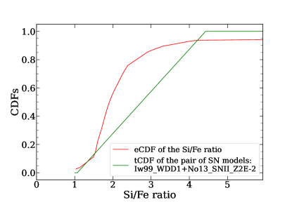
Figure 2: Comparison between the Empirical cumulative distribution function (eCDF) and Theoretical cumulative distribution function (tCDF) for the SN pair composed by Iw99_WDD1 (SNIa) and No13_SNII_Z2E-2 (SNcc). The solid red line represents the eCDF of Si/Fe abundance ratio of the groups and clusters of galaxies of our sample. The solid green line indicates the tCDF built from the pair of SNe models Iw99_WDD1 and No13_SNII_Z2E-2 (see text).

The tCDF of the pair of SN models Iw99_WDD1 (SNIa) and No13_SNII_Z2E-2 (SNcc) is presented in Figure 2 for illustration. We repeat this procedure for each one of the eight abundance ratios considered in this work and for each pair of supernova models.

4.3 Applying the KS test to the sample

Figure 2 reveals the similarity or differences between the eCDF for Si/Fe and the tCDF for Si/Fe and the pair of SN models Iw99_WDD1 (SNIa) and No13_SNII_Z2E-2 (SNcc). We quantify this (dis)similarity by Equation (10) and its p-value. Using only Si/Fe ratio, we repeated the above procedure for each of 7192 different pair combinations of SNe models, as shown in Figure 4 for some of the tested SN models. Moreover, this analysis is conducted for each one of the eight abundance ratios listed in Section 2.2, which is also represented in Figure 4. In the end, we have implemented a total of 57536 KS tests.

As mentioned previously, to reject the null hypothesis associated with the KS test, we use a threshold of 0.05. As a result, a rejected pair of SN models cannot explain our measurements of that particular abundance ratio at a 95% significance level. As we repeat this process for each of our eight abundance ratios, we can count how many times a particular pair of SN models is rejected according to the KS test. The closer this number is to 8 (total number of abundance ratios), the less representative of the data this pair of models is.

Note that in this work, we assume that there is an equal probability for an abundance ratio to have a value at any point within the predicted range of $R_{i}^{\text{Ia}}(\mathrm{E})$ and $R_{j}^{\text{cc}}(\mathrm{E})$ for a given SNIa model $i$ and a SNcc model $j$ when building its $\mathrm{tCDF}(R_{i}^{\text{Ia}}(\mathrm{E}),R_{j}^{\text{cc}}(\mathrm{E}))$. There is no theoretical reason (so far) to assume otherwise. However, this assumption may induce some perhaps unfair rejections. Among all the SN model pairs analyzed here, some outlier SN model pairs predict very wide limits in abundance ratios, and the method will tend to reject them, given that ePDFs have a more limited range. Ideally, one would have different tPDFs provided by the modelers, perhaps based on the likelihood of physical parameters used in the models. This is something to encourage the modelers to provide. Another extreme scenario that could cause undesired rejections would be if we measured the same abundance ratio for every cluster region of every cluster with extreme precision. In this case, the ePDF would be a very narrow Gaussian within the range predicted by the tPDFs, increasing the eCDF and tCDF distances. Such an unusual set of observational measurements, however, would imply that the assumption of equal probabilities along with all the theoretically “predicted” ranges would be likely incorrect. In any case, this particular anomalous case would be easily seen in the ePDF curves.

5 Published Theoretical Supernova yield models

Based on the measured ICM abundances of eighteen nearby galaxy clusters/groups, we checked the capacity of theoretical SN models to recover the observed abundance ratio distributions of our sample successfully. For that, we first built linear combinations of the fractional contribution of yields from each pair of SN models. We then verified its consistency with the distribution of observed abundance ratio measurements. The theoretical SNIa and SNcc yield models used are summarized in Tables 3 and 4, respectively. We briefly describe them here. In the model description below, all masses are in $M_{\odot}$ and $\rho_{c,9}$ is the central density in units of $10^{9}\mathrm{g~{}cm^{-3}}$).

We tested the following theoretical SNIa models:

1. The classical 1D Chandrasekhar mass ($M_{\text{Ch}}$) models (Iwamoto et al., 1999), including the “fast” deflagration models W7 and W70, as well as the delayed-detonation series of WDD and CDD models. Here, W and C are models based on a white dwarf and a carbon-oxygen core of an asymptotic giant branch star, respectively (Nomoto et al., 1984). They are artificially transformed from a subsonic to a supersonic regime based on different transition densities ($\rho_{T,7}$). In denoting the models in the tables, we follow their original notation but starting with “Iw99”.

2. 2D spherical pure deflagration (DF) model and two 2D delayed-detonation (or deflagration-detonation transition, DD) models, one of which assumes a central (denoted as “ctr”) deflagration and the other an initial off-center (denoted as “off”) deflagration (Maeda et al., 2010). We denote them as Ma10_(ctr$\mid$off)_(DF$\mid$DD), whereby (x$\mid$y$\mid$z) indicates that we choose either x or y or z to be in the displayed name.

3. 3D off-center deflagration model of Kromer et al. (2015) in a near-$M_{\text{Ch}}$ hybrid white dwarf, i.e., composed by carbon-oxygen (C+O) core and a surrounding layer of oxygen-neon (O+Ne) with five ignition spots placed randomly around the center of the WD as in Kromer et al. (2013a) and Fink et al. (2014) (denoted Kr15_hybrid).

4. A set of 3D pure deflagration models of $M_{\text{Ch}}$ C+O WD progenitor of Fink et al. (2014), where the number of ignition spots, N, varies from 1 to 1600 and with a range of central densities ($\rho_{c,9}=1-5.5$). The authors used the same setup for deflagration explosions as Seitenzahl et al. (2013) without assuming delayed-detonation. Two models initially have a very dense arrangement of the ignition kernels and are referred to as “compact” models and denoted with an additional “c” in the model name. The notation then follows Fi14_$\rho_{c,9}\_c$.

5. A set of 3D delayed-detonation models of Seitenzahl et al. (2013) assuming a range of the number of ignition spots N, which varies from 1 to 1600, central densities ($\rho_{c,9}=1-5.5$) and initial metallicities ($Z_{\rm init}=0.01-1.0Z_{\odot}$). We name the models Se13_$\rho_{c,9}$_Z$Z_{\rm init}$_c. The additional “$Z_{\rm init}$” or “c” are in the name when the initial metallicity is not a unity or if there are “compact” ignition kernels, respectively. We also included the more recent 3D gravitationally confined detonation model with one off-centered ignition spot Se16_GCD (Seitenzahl et al., 2016).

6. A set of 3D delayed-detonation $M_{\text{Ch}}$ models of Ohlmann et al. (2014), which investigates the impact of different initial carbon mass fractions ($X_{\rm C}$) on the spontaneous deflagration to detonation transition. They have deflagration ignition conditions identical to the N100 model of Seitenzahl et al. (2013). The WD progenitor has a homogeneous core or a homogeneous carbon depleted core with different $X_{\rm C}$, and we denote these models following Oh14_DD_$X_{\rm C}$.

7. A set of 2D pure turbulent deflagration models with and without transition to detonation for different central densities ($\rho_{c,9}=0.5-5.0$) and initial metallicities ($Z_{\rm init}=0-5Z_{\odot}$) of the progenitor (Leung & Nomoto, 2018). Four models assume only pure turbulent deflagration and are denoted with an additional “1P” in the model name. We then denote the models as Le18_$\rho_{c,9}\_{\rm Z}Z_{\rm init}$_1P.

8. We also consider, the sub-MCh double-detonation (DDet) models of Leung & Nomoto (2020a), for a wide range of progenitor masses ($M_{\text{WD}}=0.9-1.2$), Helium envelope masses ($M_{\text{He}}=0.05-0.1$), initial metallicities ($Z_{\rm init}=0-0.1$) and also probed carbon detonations triggered by different He detonation configurations: spherical (S), bubble (B) and ring (R) shaped. We denote their models as Le20a_$M_{\text{WD}}$_$M_{\text{He}}$_$Z_{\rm init}$_(S$\mid$B$\mid$R).

9. 2D pure turbulent deflagration models of Leung & Nomoto (2020b) for a range of initial central densities ($\rho_{c,9}=1.0-9.0$) and WD masses ($M_{\text{WD}}=1.33-1.40$) of the progenitor with solar metallicity. These models are named as Le20b_$\rho_{c,9}$_$M_{\text{WD}}$. We also include the set of hybrid C+O core WDs with an O+Ne+Mg surrounding layer (hybrid) for the same range of total masses composed by different C+O masses ($M_{\rm C+O}=0.43-0.5$) with constant oxygen and neon mass of $0.9M_{\odot}$. We name these hybrid models as Le20b_Hybrid_$M_{\rm C+O}$.

10. The 3D violent merger models of Kromer et al. (2013b, 2016) including a merger between two sub-$M_{\text{Ch}}$ WDs (with masses $0.9M_{\odot}$ and $0.76M_{\odot}$) for two different metallicities ($Z_{\rm init}=1$ and $Z_{\rm init}=0.01$). These models are respectively, named Kr13_0.9_0.76 and Kr16_0.9_0.76_Z1E-2.

11. The 3D violent merger model between two sub-$M_{\text{Ch}}$ C+O WDs of $\approx 0.9M_{\odot}$ (Pakmor et al., 2010), as well as the 3D violent merger model between two sub-$M_{\text{Ch}}$ C+O WDs of $0.9M_{\odot}$ and $1.1M_{\odot}$ (Pakmor et al., 2012), named Pr10_0.9_0.9 and Pr12_1.1_0.9, respectively.

12. The 3D models of Papish & Perets (2016) with published yields, simulating a direct collision of two sub-$M_{\text{Ch}}$ C+O WDs of $0.6M_{\odot}$, with and without the presence of a low-mass He shell of $0.01M_{\odot}$) in the WD progenitors. These models are named Pa16_1A and Pa16_1C_He, respectively.

13. 3D Dynamically-driven double-degenerate double-detonation models of Shen et al. (2018) for different progenitor masses ($M_{\text{WD}}=0.8-1.10$), carbon to oxygen ratios (${\rm C/O}=30/70$ or $50/50$), initial metallicities ($Z_{\rm init}=0-0.02$) and ${\rm{}^{12}C+^{16}O}$ reaction rates ($\text{f}_{\rm{}^{12}C+^{16}O}=0.1$ or $1.0$). The model parameters are inserted in their names following the notation Sh18_$M_{\text{WD}}$_${\rm C/O}$_$Z_{\rm init}$_$\text{f}_{\rm{}^{12}C+^{16}O}$.

14. 1D pure detonation (Det) of sub-$M_{\text{Ch}}$ C+O WD models for a range of $M_{\text{WD}}=(0.81-1.15)$, initial central densities ($\rho_{c,7}=1.0-7.9$) of the progenitor of Sim et al. (2010). We follow the notation Si10_Det_$M_{\text{WD}}$_$\rho_{c,7}$. One of the cases, Si10_Det_1.06_4.15 is also simulated for a non-zero Ne mass fraction and detonated by Si10_Det_1.06_4.15_Ne.

15. Both sets of 2D converging-shock (CS) and edge-lit (EL) double-detonation models and He only (He) detonation models of Sim et al. (2012), for two $M_{\text{WD}}$ masses of 0.66 and 0.79 $M_{\odot}$ (with a fixed $M_{\rm He}=0.21$) and central densities of $\rho_{c,7}$ of 0.38 and 0.85, for each case. We named them Si12_DDet_$M_{\text{WD}}$_$\rho_{c,7}$_(CS$\mid$EL$\mid$He).

16. The 3D delayed-detonation models of O+Ne WD for a range of masses $M_{\text{WD}}=1.18-1.25$ and central densities ($\rho_{c,9}=0.1-0.2$) of Marquardt et al. (2015). We also include their comparison model of a 1.23 M_⊙ C+O WD. We denote them as Mk15_DD_$M_{\text{WD}}$_$\rho_{c,9}$_(ONe$\mid$CO).

17. 2D and 3D centrally ignited deflagration models, as well as 3D multi-point ignition models with 5 and 30 ignition bubbles (IB) of Travaglio et al. (2004). Their WD central density, $\rho_{c,9}$, is 2.9 using a variety of linear grid sizes (GS) of 256, 512, and 768. We name the models Tr04_3D_IB_GS if the ignition bubbles are off-center and Tr04_(2D$\mid$3D)_GS if they are centered. In one of the cases, we also considered the Tr04_3D_256 for the nucleosynthesis calculations starting only at 90% of the temperature peak ($\sim 8.5\ \mathrm{x}\ 10^{9}$ K) for those tracer particles that reach nuclear statistical equilibrium (NSE) conditions. We add a “T” to its notation.

In the context of SNcc models, we test the following SNcc models assuming a Salpeter IMF (see Equation (4)):

1. Type II supernova model of Nomoto et al. (1997), which provides the IMF-weighted yields calculated for a range of $10-50M_{\odot}$ with $Z_{\rm init}=1Z_{\odot}$ and we denote by No97_SNII_Z1.

2. Three older versions of the SNII and Hypernovae (HN) models from Nomoto et al. (2006) as a function of the initial metallicity and mass of the progenitor star; The models are named No06_(SNII$\mid$HN)_$Z_{\rm init}$. Their updated models are in Table 4 referenced by Kobayashi et al. (2011).

3. A set of SNcc models including normal SNII, HN, and pair-instability SN (PISN) taken from Nomoto et al. (2013) as a function of the mass of the progenitor star (up to $40\text{M}_{\odot}$) for a range of initial metallicity ($Z_{\rm init}=0-0.05$). The PISN model has only zero initial metallicity. The models are named No13_(SNII$\mid$HN$\mid$PISN)_Z$Z_{\rm init}$. We also consider the extended version for yields normal SNII and HN models (up to $140\text{M}_{\odot}$) at $Z_{\rm init}=0$, which we denoted by No13_(SNII$\mid$HN)_Z0_ext. We also include a PISN & SNII model with a progenitor mass range from 11 to 300 M_⊙ and zero initial metallicity called No13_SNII&PISN_Z0.

4. Heger & Woosley (2002) SNII yields for $10-100\text{M}_{\odot}$ mass range and Heger & Woosley (2010) PISN yields for $140-260\text{M}_{\odot}$ denoted by He02_SNII_$Z_{\rm init}$ and He10_PISN_$Z_{\rm init}$ model, respectively. We also consider the combination of the two. They are named He10_SNII&PISN_0, for $10-260\text{M}_{\odot}$ mass range. All of the above models use $Z_{\rm init}=0$.

5. SNII yields for a $13-35\text{M}_{\odot}$ mass range of the progenitor with different metallicities ($Z_{\rm init}=0-0.02$), which correspond to models named Ch04_SNII_Z$Z_{\rm init}$ (Chieffi & Limongi, 2004).

6. A recent alternative set of SNcc models of Sukhbold et al. (2016) that provides yields for a progenitor mass range of $12.25-120\text{M}_{\odot}$ with solar metallicity. These models include neutrino transport and use the well-studied SN1987A as a calibrated point, denoted Su16_W18 and Su16_N20.

6 Results

6.1 Abundance Distributions

Table 2 presents our results of the X-ray spectral fitting for inner, outer, and entire FoV regions. We measured the elemental abundances (relative to Solar) of O, Ne, Mg, Si, S, Ar, Ca, Ni, and Fe for the eighteen groups and clusters of galaxies up to redshift 0.0391. The error-weighted average over our sample of each abundance ratio is presented in Figure 3.

By comparing Fe abundance measurements of inner and outer regions, we have confirmed the central Fe abundance enhancement using Suzaku observations for the clusters and groups of our sample (see Figure 3). The high Fe abundance in central regions compared to outer regions is consistent with our sample being composed of cool-core clusters/groups (see Section 2.1). This gradient is possibly due to a combination of effects, including ram-pressure stripping of galaxy flybys near the center of clusters, winds from the BCG, uplifting gas by AGN produced bubbles (e.g. Nulsen et al., 2002; Simionescu et al., 2009; Kirkpatrick & McNamara, 2015) or even intracluster type Ia supernovae (Omar, 2019). As mentioned previously, if the Fe gradient is coupled to an abundance ratio gradient, we can use it to improve the discriminating power of our technique. We can do this by separating observations of internal and external regions instead of using only the entire FoV measurements. Despite the obvious gain in number counts (statistics), the use of the whole FoV averages out the abundance inhomogeneities (potentially due to different enrichment types) inherent to the ICM and makes it insensitive to the real span of elemental abundance ratios. By sampling, instead, abundance measurements in internal and external regions, we maximize the observed range of abundance ratios and improve the discriminating power between the SN explosion models, which is the goal of this work.

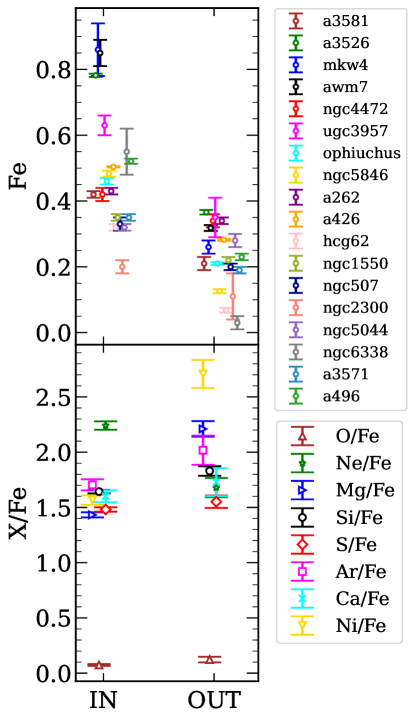
Figure 3: Top: Suzaku Fe abundance from the inner and outer regions (see text) for each group/cluster in our sample. Bottom: The error-weighted average over our sample of each abundance ratio (X/Fe) for the inner and outer regions.

Figure 3 shows the elemental abundance ratio of element “X” to iron (X/Fe) radial inner and outer region measurements. While some ratios are consistent with flat profiles, within the errors, others show indications of radial gradients within $\sim$0.2 R₂₀₀.

It is worth noticing that aside from the expected abundance ratio radial gradients mentioned above, the distribution of abundance ratios often shows significant differences not just radially but also azimuthally (e.g. Dupke et al., 2007b). These inhomogeneities also can be found at small spatial scales near the cluster core (e.g. Dupke et al., 2007a, b) and can be due to different mechanisms, e.g., core sloshing, AGN induced bubble uplifting (e.g. Churazov et al., 2001; Guo & Mathews, 2010), residual substructures from a merger, and will vary from cluster to cluster. The precise level of inhomogeneity and its causes for each cluster are scientifically interesting, but not relevant for the purposes of this work. However, even if we had the necessary spatial resolution to map the inhomogeneities in detail, it could only result in minor variations of the range of abundance ratios, which would only slightly improve the discriminating power of the method. Given that the ICM is optically thin throughout, we apply the simplest models that account for the collisionally ionized equilibrium (CIE) plasma, Galactic Hydrogen absorption, and the AGN emission, the latter being applied only to the inner and total regions. Nevertheless, as a sanity check, we compare some of our results to other works that aim to determine the phenomenological idiosyncrasies of the ICM, especially near the core. For that, we chose the Perseus cluster, overwhelmingly studied with multiple independent abundance ratio measurements, including RGS/XMM-Newton and Hitomi (Simionescu et al., 2019, hereafter S19) aside from Suzaku (Tamura et al., 2009, hereafter T09). The detailed discussion of that comparison is presented in Appendix B, where one can see that despite the differences in extracted spatial regions, spectral modeling, systematics related to the effective area, and line de-blending capabilities, our results are consistent overall with previous measurements.

Since the systems studied here exhibit positive radial temperature gradients within the regions analyzed, and they are overall “cold” it is pertinent to check the effects of the so-called Fe bias (Buote & Fabian, 1998; Buote, 2000; Gastaldello et al., 2021). In principle, one would expect this effect to be small(e.g. Rasia et al., 2008) especially using our coarse regions and extending the energy range down to 0.5 keV, which allows us to obtain a robust determination of the continuum. Nevertheless, we investigated whether neglecting the multi-temperature structure in cool groups significantly impacts the X/Fe ratio. We re-fitted the cool clusters (below kT=2 keV) with a vapec+vapec (2T) model, where the individual abundance parameters were tied between the vapec models. We found that the single vapec (1T) model measures Fe abundance was lower than the 2T model for 55% of the cool groups/clusters. In fact, the Fe error-weighted average increased from $0.553\pm 0.005$ (1T) to $0.779\pm 0.007$ (2T) for our sample of groups/clusters below 2 keV. However, the abundance ratios derived from the 2T and 1T models are generally within the errors, except for very few specific and non systematic cases, which do not affect the assessment of SN pair rankings, given the large set of abundance ratio measures to build the eCDF.

We also compare our X/Fe measurements with previous results in the literature. A brief discussion of that comparison is presented in the Appendix C, where one can see that despite using different samples, X-ray satellites, detectors, extraction regions, atomic database versions, and spectral models, the results presented here are, in general, consistent for most X/Fe measurements.

6.2 Comparison between ICM abundance ratios with Supernovae models yields

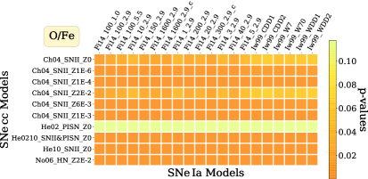
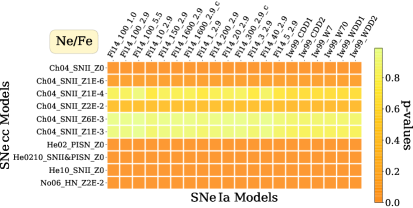
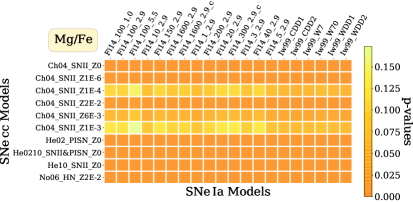
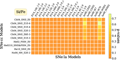
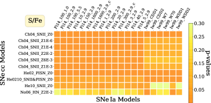
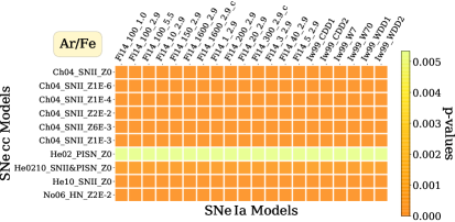
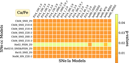
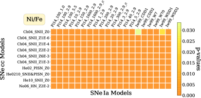
Figure 4: KS test p-values of a subset of SN model pairs (SNIa+SNcc) tested in this work using inner/outer regions for each of the eight abundance ratios (see Section 4). The color intensity map represents the values in the color bar, where more yellow cells have greater p-values. Part of SN model pairs are shown for illustration.

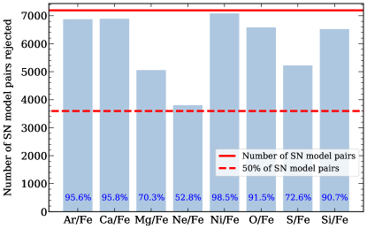
Figure 5: The number (light blue bars) and the fraction (dark blue on the bottom of the bars) of SN model pairs rejected for each abundance ratio at a 95% significance level. Solid and dashed red lines represent the total number of SN model pairs tested (7192 pairs) and its half (3,596 pairs), respectively.

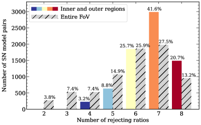
Figure 6: The amount of SN model pairs rejected by the number of rejecting ratios when using the inner/outer regions individually (colored bars) or instead, using the full FoV, denoted by “entire FoV” (gray hatched bars). The fraction of SN model pairs rejected per number of rejecting ratios (out of the 7192 SN model pairs tested) is also indicated on the top of the bars.

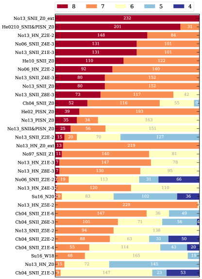
Figure 7: The number of SNIa models rejected when combined with each of the SNcc models. The number of times a SN model pair can be rejected is 8 (red), 7 (orange), 6 (yellow), 5 (light blue), and 4 (dark blue) times, as indicated by the numbers in the stacked bars. The redder the bar, the greater is the number of the most rejected pairs of SN models (i.e., the highest the rate of rejection).

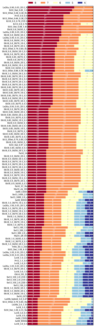
Figure 8: Same as Figure 7, but for the rejected SNcc models.

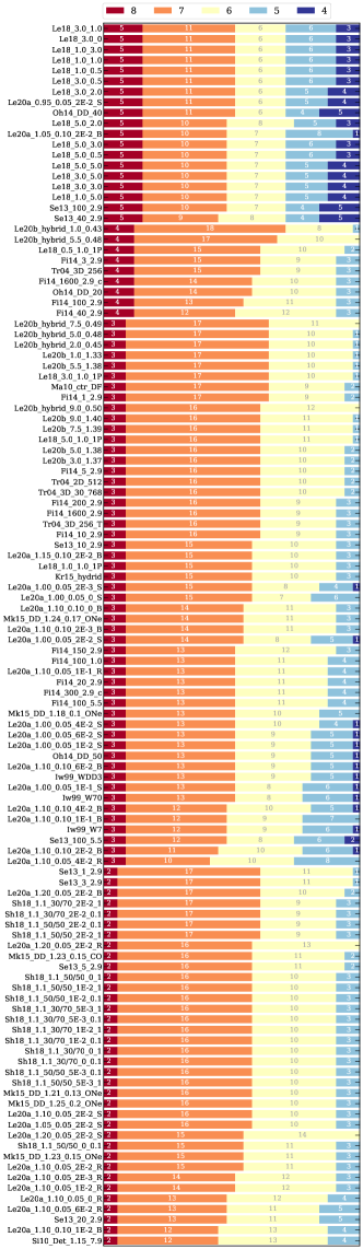
Figure 9: Continued from Figure 8

We assess the (dis)similarity of two sets of abundance ratio distributions: the ones predicted by a particular pair of SN models to those observed in the ICM/IGrM. Figure 4 shows the compilation of the p-values for each abundance ratio for some pair of SN models. In these figures, we only show a snippet of the entire figure for illustration here. The color bar represents the p-value range, increasing from yellow to orange. The color bars throughout this paper indicate the number of rejecting ratios.

We found a significant number of rejected SN model pairs by each abundance ratio individually; every abundance ratio rejected at least 50% of the total pairs (see Figure 5). In principle, one could choose a single abundance ratio as the “best” one and carry out the comparison with the SN model pairs, but this is prone to inaccuracies, given the different systematics of different detectors, such as the capacity of de-blending specific lines and different frequency range covered. Therefore, any robust comparative evaluation of SN model pairs should use as many abundance ratios as possible. Here, we used eight abundance ratios to perform this comparison without attributing reliability weights to any individual one (see Section 4).

It is important to note that the discriminative power of the method increases with the number of rejections as well as with the number of rejecting ratios. This combination is maximized when we treat inner and outer regions separately, as shown in Figure 6. Using the abundance ratios measured from the entire FoV instead of the inner and outer regions reduces the amount of rejected SN pairs at a higher number of rejecting ratios. We found that 2,989 SN pairs have been rejected by 7 (out of 8 ratios) using the inner/outer region, while only about 1,979 have been rejected by seven ratios using the entire FoV. Since this paper aims to compare and rank different pairs of SN models, the more extensive the observationally sampled range in the SNIa/SNcc contribution to ICM metal mass fraction, the higher discriminative power we have. The fact that separating the inner/outer regions increases the discriminative power of the method is consistent with the presence of radial gradients in abundance ratios. Moreover, the fact that no pair was rejected by only one ratio (or none) is consistent with the assumption that all ratios should tend to converge to a single combination of SNIa model and SNcc model mix. If the individual ratios did not converge, they would reject the pairs randomly and one could expect many ratios to reject all SN model pairs. This is not the case as shown in Figure 5, where it can be seen that the rejection number per ratio varies from 52.8% (Ne/Fe) to 98.5%(Ni/Fe). The reasons for particular individual ratios to reject pairs may be due not only to the models being inadequate but also to different intrinsic systematics related to abundance measurements, such as the conditions of the organic deposition layer and periods where Spaced-Row Charge Injection was turned on and off among the four detectors, or the ATOMDB used. The latter is especially important for ratios depending on abundances of elements measured within the L-shell region. However, here, we found no convincing indication that would lead us to systematically exclude data from any of the detectors, time periods or individual abundance ratios. In the next section, we discuss the results for the most and the least rejected pairs of SN models.

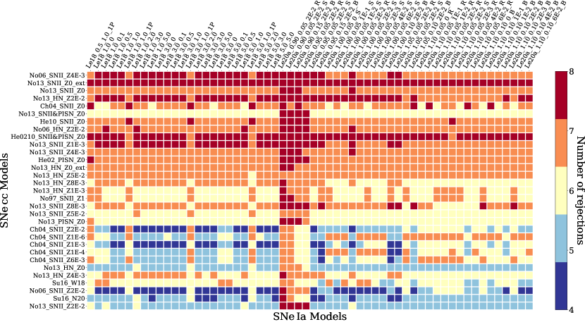
Figure 10: The number of times each SN model pair has been rejected at the 95% significance level via KS test using inner/outer regions. A pair of SN models can be rejected at a maximum of 8 times due to the 8 abundance ratios considered in this work (see Figure 4). The red and dark blue squares represent the most and least rejected pairs of SN models found in this work. The remaining results can be found in the Appendix D in Figures 14, 15 and 16.

6.2.1 The most rejected SN model pairs

The most rejected pairs of SN models have complete incompatibility with all abundance ratio distributions. They correspond to about $21\%$ of the total pairs of SN models tested (i.e., 1,489 pairs) and, we indicate them in red color throughout this paper (e.g., Figure 7). In the following, we highlight some general common trends noticed. We show the main results in Figures 7–9.

Figure 7 indicates the number of SNIa models that are rejected when combined with a particular SNcc model; the color bar represents the number of rejecting ratios that the corresponding SN pair is rejected at a 95% significance level. The No13_SNII_Z0_ext (SNcc) model paired with each one of the 232 SNIa models has the maximum rejection number that our test can obtain. It represents a Type II Supernova model with zero initial metallicity progenitor stars ($Z_{\rm init}=0$), where the average yield spans from $11$ to $140$ $\text{M}_{\odot}$. Even within the wide range of SNIa models tested, all SN pairs that include the No13_SNII_Z0_ext model provide a poor correspondence of the observed abundance ratio pattern of the ICM/IGrM analyzed here. We note that in this case, the only stellar yields available above 40M_⊙ are 100M_⊙ and 140M_⊙. As a result of this limitation, the final yield integration (Eq. (4)) may be affected by the IMF weighting for the broad-spaced mass binning applied within the 40-140M_⊙ interval mass (Mernier et al., 2017). Therefore, one could compare it with the No13_SNII_Z0 model instead, in which the progenitor’s mass upper limit is 40M_⊙. Despite the slight performance improvement for the No13_SNII_Z0 SNcc model, where the number of the most rejected combinations drops from 232 to 80, the 152 remaining pairs are still notably incompatible for all ratios except Ca/Fe. Even though these family models’ performance changes with the initial metallicity, no clear trend could be found.

The performance of SN pairs that include pair-instability SN (PISN) yields is significantly poorer (in the bottom 50%) than other types of SNcc models, none of them being rejected by less than six abundance ratios. In particular, the theoretical Ni/Fe, Ca/Fe, Si/Fe, and Ne/Fe ratios (and also S/Fe most of the time) of these pairs are entirely incompatible with the observed ratio distributions of our sample. For instance, SN pairs including the SNII & PISN yields of (Heger & Woosley, 2002, 2010) (He0210_SNII&PISN_Z0) are rejected 201 times for all abundance ratios tested (red bars in Figure 7) whereas, the remaining 31 pairs are still rejected significantly by 7 ratios, except for S/Fe (orange bars in Figure 7). This result suggests that PISNe, as characterized by their predicted elemental yields, are less likely to contribute to the chemical enrichment of the ICM as other models, based on the ICM measurements taken from our sample and on the PISN models considered.

Analogously, it may be insightful to look also at the most rejected SNIa models. Interestingly, no individual SNIa model was rejected by all abundance ratios when paired with each one of all SNcc models (see Figure 8). However, one can see from Figures 8 and 9 that nine SNIa models were rejected by at least 7 ratios for all combinations tested (red and orange bars). Two 3D violent C+O WDs merger models (Pr10_0.9_0.9 & Kr16_0.9_0.76_Z1E-2), two 2D double-detonation models both with $M_{\text{WD}}=0.90$ but with different He detonation configurations (Le20a_0.90_0.05_2E-2_R & Le20a_0.90_0.05_2E-2_S), two pure detonation 1D sub-Chandrasekhar mass C+O WDs models (Si10_Det_0.81_1.0 & Si10_Det_0.88_1.45), two 2D double-detonation models with different initial detonation configurations (Si12_DDet_0.66_0.38_EL & Si12_DDet_0.66_0.38_CS) and a 1D dynamically-driven double-degenerate double-detonation model with high ${\rm{}^{12}C+^{16}O}$ reaction rate (Sh18_0.8_50/50_0_1).

By comparing how the variants (parameter values) of the mentioned SN models have performed, we can draw some conclusions about the possible commonalities that could explain the high rejection level. Out of the four violent merger models, the one that fared well was Pr12_1.1_0.9 (Pakmor et al., 2012), a merger of two WDs of $0.9M_{\odot}$ and $1.1M_{\odot}$. All other violent merger models where both WD masses were $\leq 0.9M_{\odot}$ were highly rejected. There was a tendency to be less rejected as WD masses got larger: $\geq 0.9M_{\odot}$ for the double-detonation models of Leung & Nomoto (2020a), $\geq 1.06M_{\odot}$ for the pure detonation models of Sim et al. (2010) and $\geq 0.79M_{\odot}$ for all cases of the double-detonation models of Sim et al. (2012). Although a similar trend can be seen in the double-degenerate double-detonation models of Shen et al. (2018) for low masses, the 1 M_⊙ models outperformed the 1.1 M_⊙ ones.

The complete rejecting maps of all pairs of SN models tested in this work are presented in Figure 10 and in the Appendix D in Figures 14, 15 and 16.

6.2.2 The least rejected SN model pairs

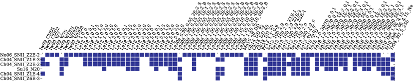
Figure 11: Subset of 229 SN pairs (SNIa+SNcc) ranked as the least rejected pairs of SN models in this work (dark blue). The blank squares refer to the SN pairs rejected by more than four abundance ratios.

In this section, we analyze the subset of pairs of SN models rejected only 4 out of 8 times tested, which are the least rejected pairs found (see Figure 11). It is worth stressing again that when a pair of models is rejected repeatedly, we can conclude that this pair does not represent the observations satisfactorily. On the other hand, even if a pair of models is not systematically rejected, one can only conclude that the observed data set provides insufficient evidence against the null hypothesis. As a result, one cannot formally state that the pair is the best fit for the observed data. As in the previous section, we can highlight some common trends among the SN models that fared best for ICM enrichment studies.

Figure 6 shows that only 229 (out of 7192) SN model pairs are rejected only by 4 abundance ratios, when paired within the set of SNIa models (see dark blue bars in Figure 7), corresponding to a small fraction of $\sim 3.2\%$ of the total number of pairs tested in this study. Among them, we identified only 6 (out of 31) different SNcc models: the Nomoto et al. (2006) Type II model with $Z_{\rm init}=2$E-2, four Type II models from Chieffi & Limongi (2004) with 1E-4$\leq Z_{\rm init}\leq$2E-2 and a nonrotating model calibrated for SN1987A with $Z_{\rm init}=1Z_{\odot}$ (Sukhbold et al., 2016).

All models above are SNcc models with nonzero initial metallicity progenitor stars exploding as Type II Supernova, which outperforms PISN and Hypernova models with any initial metallicity and also Type II Supernovae with $Z_{\rm init}=0$. The total number of SNIa models combined with each SNcc model mentioned above with only 4 rejection ratios are 66, 53, 50, 36, 20, and 4, respectively (see Figure 7). Since our work ranks SN model pairs and not individual models, it is interesting to look at the “flexibility” of the SNIa models individually to maximize the number of SN pairs that rank best in the least-rejected-pair space. Doing so, we notice that the 3D delayed-detonation models of Seitenzahl et al. (2013) with 40-150 ignition spots for central densities ($\rho_{c,9}=2.9$) and initial metallicities ($Z_{\rm init}\neq 0$), the delayed-detonation models of Ohlmann et al. (2014) with 100 near-center ignition spots for carbon depleted core WD (Oh14_DD_32/40), and also the gravitationally confined detonation model with one off-centered ignition spot of Seitenzahl et al. (2016) outperform all other matches when paired with the SNcc models listed above. In addition, the Ch04_SNII_Z6E-3 model performed equally well when paired with 3D multi-point ignition, five bubbles, and $\rho_{c,9}=2.9$ model of Travaglio et al. (2004).

7 Conclusions

We have determined O/Fe, Ne/Fe, Mg/Fe, Si/Fe, S/Fe, Ar/Fe, Ca/Fe, and Ni/Fe elemental abundance ratios in the inner, outer, and entire FoV regions ($\sim$0.2 R₂₀₀) of 18 nearby clusters and groups of galaxies ($z\leq 0.0391$) with XIS/Suzaku observations, which were subsequently used to compare how well the predicted yields of different combinations of SNe yield models (i.e., an SNcc and an SNIa model) recover the observed abundance ratios in the intracluster medium. By implementing the developed non-parametric analysis based on the KS test, we ranked 7192 SNe explosion yields models from the literature using these eight different abundance ratios.

Our methodology reinforces the potential that X-ray spectroscopy of the intracluster gas has to rank among the variety of SNe yield models in the literature. Despite the purely statistical nature of the method, it provides a helpful general guidance to those interested in both the chemical enrichment mechanisms in galaxy clusters and those interested in the nature of supernova progenitor systems and explosion mechanisms. Our main findings can be summarized as follows.

1. We confirm the Fe central abundance enhancement for our sample, even for those systems where the cool-core is not easily resolved, suggesting that the Fe abundance (negative) gradient has a shallower profile than that of the temperature (positive) gradient (see Table 2).

2. By building probability distributions for each elemental abundance ratio measurement, we quantified the degree of incompatibility between the prediction by each pair of SN models and the observations. More than half of the total number of SN pairs are rejected by each abundance ratio individually (see Figure 5) and $\approx 21\%$ of the total pairs of SN models tested (i.e., 1489 SN pairs) have complete incompatibility with all abundance ratio distributions (see Figure 6).

3. The separate measurements of clusters’ inner and outer regions enhance the discriminative power of our technique among the 7192 SN model pairs tested (see Figure 6). This is consistent with the premise of abundance ratio gradients in the central regions of cool-core clusters and groups, as raised by different authors previously.

4. Among the 7192 different SN model pairs tested, all 232 SN model combinations that include No13_SNII_Z0_ext are rejected by all abundance ratios (see Figure 7). This model simulates a Type II Supernova with zero initial metallicity progenitor stars ($Z_{\rm init}=0$) for yield mass range from $11$ to $140\text{M}_{\odot}$. On the other hand, no SNIa model paired with all 31 SNcc models, achieves the highest rejection number (see Figures 8 and 9).

5. Overall, PISN and Hypernova models with any initial metallicity and Type II Supernova models with $Z_{\rm init}=0$ do not predict the observed abundances as well as Type II Supernova with nonzero initial metallicity progenitors.

6. Narrowing down to the least rejected pairs of SN models, we see that 3D models where the WD progenitor central density of $2.9\times 10^{9}\,{\rm gcm^{-3}}$ seem to dominate. Among them, Ohlmann et al. (2014) delayed-detonation models with 100 near-center ignition spots, for carbon depleted core (Oh14_DD_32/40), Seitenzahl et al. (2013) delayed-detonation models with 40-150 near-center ignition spots and their one-ignition, and Seitenzahl et al. (2016) gravitationally confined detonation model (Se16_GCD) are more observationally robust, in the sense of predicting the range of the observed abundance ratios and so is the off-center 5-bubble ignition of Travaglio et al. (2004) (Tr04_3D_5_256)(see Table 3).

   On the SNcc side, among the least rejected pairs, we find Nomoto et al. (2006) Type II model with $Z_{\rm init}=2$E-2, four Type II models from Chieffi & Limongi (2004) with $1{\rm E}-4\leq Z_{\rm init}\leq 2{\rm E}-2$ and a nonrotating model calibrated for SN1987A with $Z_{\rm init}=1Z_{\odot}$ (Sukhbold et al., 2016) (see Table 4 and Section 5 for main characteristics about SN models tested in this work).

7. The results favor the scenario where the massive progenitor stars of core-collapse Supernova that contributed significantly to the ICM enrichment must have been initially enriched. The zero metallicity SNcc models ($Z_{\rm init}=0$) do not reasonably reproduce the ICM abundance ratios distribution pattern, independent of the SNIa pairing choice. Also, the results suggest the origin of the majority of the intracluster gas metal enriching SNIa as near-Chandrasekhar mass progenitors with near-center, multiple ignition spots.

The PDF non-parametric analysis carried out in this work is a potentially powerful tool to constrain competing SNe explosion models. This technique will become more and more refined as the number of ICM abundance measurements grows, as the spectral resolution improves, and as the number of predicted yields from different types of SN are made available. Hence, the algorithm is suitable for new X-ray measurements and SN models, as they appear in the literature. The analysis is robust because we are not “picking and choosing” the preferred ratios, even though the method is open to the implementation of particular sets of weights to individual ratios based on information on the instrument efficiency, background contamination susceptibility, and energy range used, etc. This analysis can be helpful to the cluster and the SNe communities, serving as a guide to improving SN models based on observations and helping to choose the most adequate set of SN models to analyze many critical problems related to metal enrichment in clusters, groups, and even galaxies. In this work, no combination of SN models is fully compatible with all observed abundance ratios, even testing an extensive set of 7192 pairs of SN models. The upcoming micro-calorimeters onboard X-ray observatories will achieve more precise measurements of ICM abundances of (rare) elements, allowing better discrimination among SNe models enriching the ICM (e.g. Mernier et al., 2020). The power of XRISM Resolve high-resolution spectroscopy (XRISM Science Team, 2020) will enable accurate measurements of elements such as Cr and Mn in the ICM for multiple nearby systems within the next few years. Incorporating these different abundance ratios in this analysis can better constrain SN models by having accurate measurement abundances of these and other elements and different abundance ratios. By combining low and stable detector background, high effective area, and large FoV, the Advanced X-ray Imaging Satellite (AXIS) camera (Mushotzky et al., 2019) will provide measurements of abundance with low particle background and an overwhelmingly better spatial resolution than Suzaku, offering invaluable information to map the enrichment in different cluster regions. Complementary, the X-IFU Athena (Pointecouteau et al., 2013) will trace the detailed metal distribution in these systems at high redshifts (z$\sim$2) and allow us to explore the nearby systems at unprecedented distances (Cucchetti et al., 2018). It will be crucial to investigate the role of pre-enrichment in the history of metal enrichment mechanisms. Compiling these achievements with this analysis should provide significantly better constraints on the variety of SN models and serve as a testbed for the different physical ingredients input in the SN simulations.

Appendix A Probability distribution functions for abundance ratios used in this work

This section presents the probability distribution functions for other abundance ratios used throughout this work. Figure 12 illustrates the PDFs from both inner and outer regions (solid blue lines) for each object and the combined PDF distribution (solid red lines).

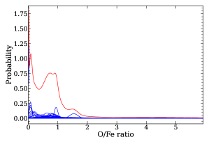
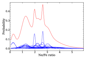
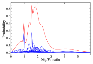
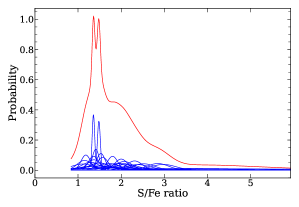
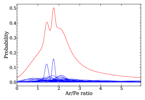
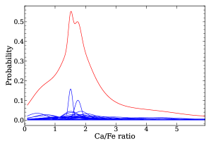
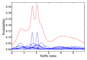
Figure 12: Same as Figure 1 for each X/Fe abundance ratio measurements.

Appendix B Comparison of Perseus measurements with previous results

Here we estimate the impact of averaging out the possible idiosyncratic phenomenologies of the ICM near the core on the abundance measurements, due to Suzaku’s limited spatial resolution. We chose the Perseus cluster as the golden case for comparison because it has been overwhelmingly studied with multiple independent abundance measurements, including the XMM-Newton RGS, Hitomi (Simionescu et al., 2019, hereafter S19) and also Suzaku (Tamura et al., 2009, hereafter T09).

T09 have measured several abundance ratios in the central regions of the Perseus cluster with Suzaku, using the observation taken in Feb 2006 (that we used in this work) and seven more pointings taken for calibration purposes between Aug. 2006 and Feb 2009. Their results for the two central bins within the central $4\arcmin$ are very similar to each other, which is not surprising given that they are effectively within Suzaku’s PSF. Their observed abundance ratios generally agree with what we found for a single absorbed CIE model, except for the Ne/Fe ratio. We found a higher Ne/Fe value even considering the $\sim 25\%$ systematic errors suggested by T09 to account for the simultaneous fittings of all instruments and observations in their work. Our measured Ne/Fe ratio becomes compatible with the values obtained by T09 when we use a two-temperature model (with the same spectral fitting setup as that of T09). However, as we mentioned previously, a more complex spectral fitting model is not justified in our work since a detailed mapping of the ICM thermal inhomogeneities is not our goal. In the worst-case scenario, this would increase the span covered by the Ne/Fe ratio values, making that index less discriminative than the others. Indeed, the Ne/Fe ratio has the lowest impact on our analyses since it is the most irrelevant ratio to indicate the discrepancies between the SN model pairs (see Ne/Fe ratio in Figure 5). The evaluation of the most rejected pair of models relies not only on Ne/Fe but also on seven other ratios. Moreover, excluding Ne/Fe from the analysis increases the absolute number of the least rejected pairs of SN models (i.e., incompatible with only four ratios – see section 6.2.2) from 229 to 238. It corresponds to only a slight change from $\approx 3.2\%$ to $3.3\%$ of the total pairs of SN models tested, respectively.

We also chose to use only the earliest Perseus observation to avoid the systematics due to the contamination layer of the filters, which is stronger in lower frequencies and may artificially influence the measurements of the abundances of O and Ne. The amplitude and scatter of the degradation of the soft-energy effective area due to the organic contamination layer in the optical path of each sensor of Suzaku is well documented (Petre, 2008) also in The Suzaku Data Reduction Guide v5.0, and affects more strongly the late (post 2006) observations, which were included in both Tamura et al. (2009) and Simionescu et al. (2019).

The Hitomi satellite carried on-board a high-resolution spectrometer, which unfortunately stopped working during the commissioning phase in 2016. However, it partially observed the core of the Perseus cluster with four pointings, three overlapping in the central $\sim 2^{\prime}-3^{\prime}$, and an offset pointing about 4^′ SW of the center (Hitomi Collaboration et al., 2018). S19 performed an analysis of the metallicity of the Perseus core using data from Hitomi (above 2 keV), Suzaku (all available pointings to date), and XMM-Newton, including the RGS for abundances measured below 2 keV.

When comparing the results from S19 to our analysis of the main Suzaku pointing of Perseus, one should keep in mind that, even with the large PSF of Suzaku (and Hitomi), S19 so-called Hitomi’s “entire core” region is asymmetrically configured and reaches at most $\sim 3^{\prime}$ distance from the center. In area, it is $\sim$ 50% smaller than our central region and significantly larger (by 4 to 5 times) than that analyzed with the RGS. One notable discrepancy likely due to the differences in extraction regions is the Fe abundance, which is measured to be $0.46\pm 0.05$ (RGS/XMM-Newton), $0.71\pm 0.003$ (this work, but with the same spectral models as that of S19), $0.81\pm 0.01$ (Hitomi), and $0.821\pm 0.001$ (Suzaku) in solar units converted from Lodders et al. (2009), used in their paper, for proper comparison.

The Fe abundance distribution in Perseus is known to have an overall negative radial gradient first noted by Ulmer et al. (1987) and later confirmed by many different works (e.g. Ponman et al., 1990; Dupke & Arnaud, 2001; Simionescu et al., 2011; Ueda et al., 2013). Also, it has significant anisotropic inhomogeneities measured with Chandra (Sanders et al., 2004). The slight differences between the Fe abundances measured by us with Suzaku and with Hitomi are not surprising, given the presence of a radial Fe abundance gradient. However, the discrepant lower Fe abundance measured by the RGS is puzzling and possibly related to the degeneracy between the Fe absolute abundance and the normalization of the CIE component due to the RGS limited wavelength coverage (S19).

The best-fit values of Ne/Fe, Mg/Fe, and Ni/Fe ratios obtained by us agree with those from the RGS, while the O/Fe ratio is somewhat smaller. de Plaa et al. (2017) extensively discusses the systematics affecting the O/Fe ratio with the RGS, and we refer the reader to that work. However, given the very small area of analysis of the RGS (basically the central $10\,{\rm kpc}$), it cannot be ruled out that this discrepancy could be caused by a large amount of dips and peaks of the individual elemental abundances in that region near the core (Sanders et al., 2004). In addition, if we fix the value of the Fe abundance to that of Hitomi, which is measured in the Fe-K complex and very reliable, the O/Fe ratio measured by RGS becomes entirely consistent with our measured values. Analogously, if we fix the Fe abundance of Hitomi as the “golden” value and use it to compensate for the possible impact of the central Fe abundance gradient in our measurements with Suzaku, the abundance ratios of Si, S, and Ni to Fe become entirely consistent, while Ca and Ar to Fe become marginally consistent with those derived by our work. Therefore, we consider the overall consistency with previous measurements satisfactory.

Appendix C Comparison between abundance ratio measurements from the literature with our measurements

We compare the results of T09 and S19 from the Perseus cluster in detail in Appendix B, showing a satisfactory agreement with ours. Even though we cannot compare our measurements directly to previous works as closely as we could with Perseus, we can do a “general” comparison using a common solar abundance table. We converted our abundance ratio measurements from photospheric solar ANGR to proto-solar Lodders et al. (2009, hereafter L09), used by Mernier et al. (2016, 2018b) and S19. Similarly, we also converted the measurements of de Plaa et al. (2007) from proto-solar Lodders (2003) to proto-solar L09. After doing the proper abundance table conversion, we show the comparison in Figure 13, where we use the ‘entire FoV’ (all) region. In Figure 13, indeed, Mg/Fe, S/Fe, Ar/Fe, and Ni/Fe measurements are directly consistent with those from Mernier et al. (2016, 2018b) and S19. There are some discrepant ratios, which can be due to several reasons, including the sample choice. For example, the error-weighted average of the Ca/Fe ratio becomes about unity (0.997$\pm$0.03 Z_⊙) when ratios of NGC 4472 and 5846 groups are not considered. Overall, this illustrates the need for caution when comparing our results to others, which use different samples, satellites, detectors, extraction regions, atomic database versions, and spectral models. Even though a detailed comparison with those other works could be enlightening, it is beyond the scope of the proposed work. In any case, it is important to note that the proposed methodology does not depend on solar abundance table choice.

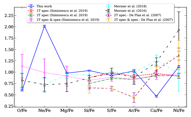
Figure 13: Comparison between abundance ratio measurements from the literature with our measurements from the entire FoV (triangle symbol connected by the solid blue line).

Appendix D The complete evaluation of SN pairs of models in this work.

Here, we present the complete result obtained in this work and partially shown in Figure 10. It represents the number of times a pair of SNIa+SNcc models has been rejected at the 95% level of significance via the KS test using the inner and outer regions. A certain pair of SN models can be rejected at a maximum of 8 times due to the 8 abundance ratios considered in this work (see Figure 4). The red squares represent the most rejected pairs of SN models in this work. Figures 14, 15 and 16 together with Figure 10 are the fully rejected maps of the 7192 SN pairs tested by the eight abundance ratios.

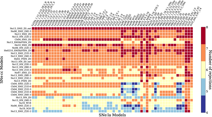
Figure 14: Continuation of Figure 10.

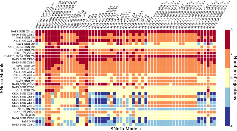
Figure 15: Continuation of Figure 10.

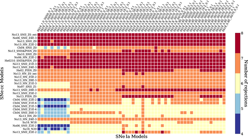
Figure 16: Continuation of Figure 10.

Appendix E List of SNe models with yields

Given the substantial number of theoretical SN model combinations tested in this work and summarized in Section 5, we present here the main remarks of each SN model collected from the literature. The nomenclature for the 232 SNIa models and 31 SNcc models in Table 3 and 4, respectively.

Table 3: List of the 232 SNIa explosion models with yields from the literature tested with our method.

Model Name	Ref.	Basic Proprieties
Fi14_1_2.9	1	3D deflagration, $\rho_{c,9}=2.9$, 1 slightly off-centre ignition bubble
Fi14_3_2.9	1	3D deflagration, $\rho_{c,9}=2.9$, 3 centred ignition bubbles
Fi14_5_2.9	1	3D deflagration, $\rho_{c,9}=2.9$, 5 centred ignition bubbles
Fi14_10_2.9	1	3D deflagration, $\rho_{c,9}=2.9$, 10 centred ignition bubbles
Fi14_20_2.9	1	3D deflagration, $\rho_{c,9}=2.9$, 20 centred ignition bubbles
Fi14_40_2.9	1	3D deflagration, $\rho_{c,9}=2.9$, 40 centred ignition bubbles
Fi14_100_5.5	1	3D deflagration, $\rho_{c,9}=5.5$, 100 centred ignition bubbles
Fi14_100_2.9	1	3D deflagration, $\rho_{c,9}=2.9$, 100 centred ignition bubbles
Fi14_100_1.0	1	3D deflagration, $\rho_{c,9}=1.0$, 100 centred ignition bubbles
Fi14_150_2.9	1	3D deflagration, $\rho_{c,9}=2.9$, 150 centred ignition bubbles
Fi14_200_2.9	1	3D deflagration, $\rho_{c,9}=2.9$, 200 centred ignition bubbles
Fi14_300_2.9_c	1	3D deflagration, $\rho_{c,9}=2.9$, 300 compact centred ignition bubbles (highly sph. symmetry)
Fi14_1600_2.9	1	3D deflagration, $\rho_{c,9}=2.9$, 1600 centred ignition bubbles
Fi14_1600_2.9_c	1	3D deflagration, $\rho_{c,9}=2.9$, 1600 compact centred ignition bubbles (highly sph. symmetry)
Iw99_W7	2	Deflagration, $\rho_{c,9}=2.12$, $\mathbf{Z_{\rm\textbf{{init}}}}=1$
Iw99_W70	2	Deflagration, $\rho_{c,9}=2.12$, $\mathbf{Z_{\rm\textbf{{init}}}}=0$
Iw99_WDD1	2	Delayed Detonation, $\rho_{c,9}=2.12$, $\rho_{T,7}=1.7$, $\mathbf{Z_{\rm\textbf{{init}}}}=1$
Iw99_WDD2	2	Delayed Detonation, $\rho_{c,9}=2.12$, $\rho_{T,7}=2.2$, $\mathbf{Z_{\rm\textbf{{init}}}}=1$
Iw99_WDD3	2	Delayed Detonation, $\rho_{c,9}=2.12$, $\rho_{T,7}=3.0$, $\mathbf{Z_{\rm\textbf{{init}}}}=1$
Iw99_CDD1	2	Delayed Detonation, $\rho_{c,9}=1.37$, $\rho_{T,7}=1.7$, $\mathbf{Z_{\rm\textbf{{init}}}}=1$
Iw99_CDD2	2	Delayed Detonation, $\rho_{c,9}=1.37$, $\rho_{T,7}=2.2$, $\mathbf{Z_{\rm\textbf{{init}}}}=1$
Kr13_0.9_0.76	3	3D C+O WDs violent merger, $(M_{1,_{\text{WD}}},M_{2,_{\text{WD}}})=(0.9,\,0.76)$, $\mathbf{Z_{\rm\textbf{{init}}}}=1$
Kr15_hybrid	4	3D Hybrid WD deflagr. (C+O core w/ O+Ne layers), five off-centre spots, $\rho_{c,9}=2.12$
Kr16_0.9_0.76_Z1E-2	3,5	3D C+O WDs violent merger, $(M_{1,_{\text{WD}}},M_{2,_{\text{WD}}})=(0.9,\,0.76)$, $\mathbf{Z_{\rm\textbf{{init}}}}=0.01$
Le18_0.5_1.0_1P	6	2D Pure Turbulent Deflagr., $\rho_{c,9}=0.5$, $\mathbf{Z_{\rm\textbf{{init}}}}=1$, C/O=1.0
Le18_1.0_1.0_1P	6	2D Pure Turbulent Deflagr., $\rho_{c,9}=1.0$, $\mathbf{Z_{\rm\textbf{{init}}}}=1$, C/O=1.0
Le18_1.0_0	6	2D Deflagration-to-Detonation, $\rho_{c,9}=1.0$, $\mathbf{Z_{\rm\textbf{{init}}}}=0$
Le18_1.0_0.1	6	2D Deflagration-to-Detonation, $\rho_{c,9}=1.0$, $\mathbf{Z_{\rm\textbf{{init}}}}=0.1$
Le18_1.0_0.5	6	2D Deflagration-to-Detonation, $\rho_{c,9}=1.0$, $\mathbf{Z_{\rm\textbf{{init}}}}=0.5$
Le18_1.0_1.0	6	2D Deflagration-to-Detonation, $\rho_{c,9}=1.0$, $\mathbf{Z_{\rm\textbf{{init}}}}=1.0$
Le18_1.0_2.0	6	2D Deflagration-to-Detonation, $\rho_{c,9}=1.0$, $\mathbf{Z_{\rm\textbf{{init}}}}=2.0$
Le18_1.0_3.0	6	2D Deflagration-to-Detonation, $\rho_{c,9}=1.0$, $\mathbf{Z_{\rm\textbf{{init}}}}=3.0$
Le18_1.0_5.0	6	2D Deflagration-to-Detonation, $\rho_{c,9}=1.0$, $\mathbf{Z_{\rm\textbf{{init}}}}=5.0$
Le18_3.0_1.0_1P	6	2D Pure Turbulent Deflagr., $\rho_{c,9}=3.0$, $\mathbf{Z_{\rm\textbf{{init}}}}=1.0$, C/O=1.0
Le18_3.0_0	6	2D Deflagration-to-Detonation, $\rho_{c,9}=3.0$, $\mathbf{Z_{\rm\textbf{{init}}}}=0$
Le18_3.0_0.1	6	2D Deflagration-to-Detonation, $\rho_{c,9}=3.0$, $\mathbf{Z_{\rm\textbf{{init}}}}=0.1$
Le18_3.0_0.5	6	2D Deflagration-to-Detonation, $\rho_{c,9}=3.0$, $\mathbf{Z_{\rm\textbf{{init}}}}=0.5$
Le18_3.0_1.0	6	2D Deflagration-to-Detonation, $\rho_{c,9}=3.0$, $\mathbf{Z_{\rm\textbf{{init}}}}=1.0$
Le18_3.0_2.0	6	2D Deflagration-to-Detonation, $\rho_{c,9}=3.0$, $\mathbf{Z_{\rm\textbf{{init}}}}=2.0$
Le18_3.0_3.0	6	2D Deflagration-to-Detonation, $\rho_{c,9}=3.0$, $\mathbf{Z_{\rm\textbf{{init}}}}=3.0$
Le18_3.0_5.0	6	2D Deflagration-to-Detonation, $\rho_{c,9}=3.0$, $\mathbf{Z_{\rm\textbf{{init}}}}=5.0$
Le18_5.0_1.0_1P	6	2D Pure Turbulent Deflagr., $\rho_{c,9}=5.0$, $\mathbf{Z_{\rm\textbf{{init}}}}=1.0$, C/O=1.0
Le18_5.0_0	6	2D Deflagration-to-Detonation, $\rho_{c,9}=5.0$, $\mathbf{Z_{\rm\textbf{{init}}}}=0$
Le18_5.0_0.1	6	2D Deflagration-to-Detonation, $\rho_{c,9}=5.0$, $\mathbf{Z_{\rm\textbf{{init}}}}=0.1$
Le18_5.0_0.5	6	2D Deflagration-to-Detonation, $\rho_{c,9}=5.0$, $\mathbf{Z_{\rm\textbf{{init}}}}=0.5$
Le18_5.0_1.0	6	2D Deflagration-to-Detonation, $\rho_{c,9}=5.0$, $\mathbf{Z_{\rm\textbf{{init}}}}=1.0$
Le18_5.0_2.0	6	2D Deflagration-to-Detonation, $\rho_{c,9}=5.0$, $\mathbf{Z_{\rm\textbf{{init}}}}=2.0$
Le18_5.0_3.0	6	2D Deflagration-to-Detonation, $\rho_{c,9}=5.0$, $\mathbf{Z_{\rm\textbf{{init}}}}=3.0$
Le18_5.0_5.0	6	2D Deflagration-to-Detonation, $\rho_{c,9}=5.0$, $\mathbf{Z_{\rm\textbf{{init}}}}=5.0$
Le20a_1.10_0.10_0_B	7	2D Double-Deton., $M_{\text{WD}}=1.10$, $M_{\text{He}}=0.10$, $Z_{\rm init}=0$, one He deton. bubble
Le20a_1.10_0.10_2E-3_B	7	2D Double-Deton., $M_{\text{WD}}=1.10$, $M_{\text{He}}=0.10$, $Z_{\rm init}=0.002$, one He deton. bubble
Le20a_1.10_0.10_1E-2_B	7	2D Double-Deton., $M_{\text{WD}}=1.10$, $M_{\text{He}}=0.10$, $Z_{\rm init}=0.01$, one He deton. bubble
Le20a_1.10_0.10_2E-2_B	7	2D Double-Deton., $M_{\text{WD}}=1.10$, $M_{\text{He}}=0.10$, $Z_{\rm init}=0.02$, one He deton. bubble
Le20a_1.10_0.10_4E-2_B	7	2D Double-Deton., $M_{\text{WD}}=1.10$, $M_{\text{He}}=0.10$, $Z_{\rm init}=0.04$, one He deton. bubble
Le20a_1.10_0.10_6E-2_B	7	2D Double-Deton., $M_{\text{WD}}=1.10$, $M_{\text{He}}=0.10$, $Z_{\rm init}=0.06$, one He deton. bubble
Le20a_1.10_0.10_1E-1_B	7	2D Double-Deton., $M_{\text{WD}}=1.10$, $M_{\text{He}}=0.10$, $Z_{\rm init}=0.1$, one He deton. bubble
Le20a_1.10_0.05_0_R	7	2D Double-Deton., $M_{\text{WD}}=1.10$, $M_{\text{He}}=0.05$, $Z_{\rm init}=0$, He deton. ring
Le20a_1.10_0.05_2E-3_R	7	2D Double-Deton., $M_{\text{WD}}=1.10$, $M_{\text{He}}=0.05$, $Z_{\rm init}=0.002$, He deton. ring
Le20a_1.10_0.05_1E-2_R	7	2D Double-Deton., $M_{\text{WD}}=1.10$, $M_{\text{He}}=0.05$, $Z_{\rm init}=0.01$, He deton. ring
Le20a_1.10_0.05_2E-2_R	7	2D Double-Deton., $M_{\text{WD}}=1.10$, $M_{\text{He}}=0.05$, $Z_{\rm init}=0.02$, He deton. ring
Le20a_1.10_0.05_4E-2_R	7	2D Double-Deton., $M_{\text{WD}}=1.10$, $M_{\text{He}}=0.05$, $Z_{\rm init}=0.04$, He deton. ring
Le20a_1.10_0.05_6E-2_R	7	2D Double-Deton., $M_{\text{WD}}=1.10$, $M_{\text{He}}=0.05$, $Z_{\rm init}=0.06$, He deton. ring
Le20a_1.10_0.05_1E-1_R	7	2D Double-Deton., $M_{\text{WD}}=1.10$, $M_{\text{He}}=0.05$, $Z_{\rm init}=0.1$, He deton. ring
Le20a_1.00_0.05_0_S	7	2D Double-Deton., $M_{\text{WD}}=1.00$, $M_{\text{He}}=0.05$, $Z_{\rm init}=0$, spherical He deton.
Le20a_1.00_0.05_2E-3_S	7	2D Double-Deton., $M_{\text{WD}}=1.00$, $M_{\text{He}}=0.05$, $Z_{\rm init}=0.002$, spherical He deton.
Le20a_1.00_0.05_1E-2_S	7	2D Double-Deton., $M_{\text{WD}}=1.00$, $M_{\text{He}}=0.05$, $Z_{\rm init}=0.01$, spherical He deton.
Le20a_1.00_0.05_2E-2_S	7	2D Double-Deton., $M_{\text{WD}}=1.00$, $M_{\text{He}}=0.05$, $Z_{\rm init}=0.02$, spherical He deton.
Le20a_1.00_0.05_4E-2_S	7	2D Double-Deton., $M_{\text{WD}}=1.00$, $M_{\text{He}}=0.05$, $Z_{\rm init}=0.04$, spherical He deton.
Le20a_1.00_0.05_6E-2_S	7	2D Double-Deton., $M_{\text{WD}}=1.00$, $M_{\text{He}}=0.05$, $Z_{\rm init}=0.06$, spherical He deton.
Le20a_1.00_0.05_1E-1_S	7	2D Double-Deton., $M_{\text{WD}}=1.00$, $M_{\text{He}}=0.05$, $Z_{\rm init}=0.1$, spherical He deton.
Le20a_0.90_0.15_2E-2_B	7	2D Double-Deton., $M_{\text{WD}}=0.90$, $M_{\text{He}}=0.15$, $Z_{\rm init}=0.02$, one He deton. bubble
Le20a_0.95_0.15_2E-2_B	7	2D Double-Deton., $M_{\text{WD}}=0.95$, $M_{\text{He}}=0.15$, $Z_{\rm init}=0.02$, one He deton. bubble
Le20a_1.00_0.10_2E-2_B	7	2D Double-Deton., $M_{\text{WD}}=1.00$, $M_{\text{He}}=0.10$, $Z_{\rm init}=0.02$, one He deton. bubble
Le20a_1.05_0.10_2E-2_B	7	2D Double-Deton., $M_{\text{WD}}=1.05$, $M_{\text{He}}=0.10$, $Z_{\rm init}=0.02$, one He deton. bubble
Le20a_1.15_0.10_2E-2_B	7	2D Double-Deton., $M_{\text{WD}}=1.15$, $M_{\text{He}}=0.10$, $Z_{\rm init}=0.02$, one He deton. bubble
Le20a_1.20_0.05_2E-2_B	7	2D Double-Deton., $M_{\text{WD}}=1.20$, $M_{\text{He}}=0.05$, $Z_{\rm init}=0.02$, one He deton. bubble
Le20a_0.90_0.05_2E-2_R	7	2D Double-Deton., $M_{\text{WD}}=0.90$, $M_{\text{He}}=0.05$, $Z_{\rm init}=0.02$, He deton. ring
Le20a_0.95_0.05_2E-2_R	7	2D Double-Deton., $M_{\text{WD}}=0.95$, $M_{\text{He}}=0.05$, $Z_{\rm init}=0.02$, He deton. ring
Le20a_1.00_0.05_2E-2_R	7	2D Double-Deton., $M_{\text{WD}}=1.00$, $M_{\text{He}}=0.05$, $Z_{\rm init}=0.02$, He deton. ring
Le20a_1.05_0.05_2E-2_R	7	2D Double-Deton., $M_{\text{WD}}=1.05$, $M_{\text{He}}=0.05$, $Z_{\rm init}=0.02$, He deton. ring
Le20a_1.20_0.05_2E-2_R	7	2D Double-Deton., $M_{\text{WD}}=1.20$, $M_{\text{He}}=0.05$, $Z_{\rm init}=0.02$, He deton. ring
Le20a_0.90_0.05_2E-2_S	7	2D Double-Deton., $M_{\text{WD}}=0.90$, $M_{\text{He}}=0.05$, $Z_{\rm init}=0.02$, spherical He deton.
Le20a_0.95_0.05_2E-2_S	7	2D Double-Deton., $M_{\text{WD}}=0.95$, $M_{\text{He}}=0.05$, $Z_{\rm init}=0.02$, spherical He deton.
Le20a_1.05_0.05_2E-2_S	7	2D Double-Deton., $M_{\text{WD}}=1.05$, $M_{\text{He}}=0.05$, $Z_{\rm init}=0.02$, spherical He deton.
Le20a_1.10_0.05_2E-2_S	7	2D Double-Deton., $M_{\text{WD}}=1.10$, $M_{\text{He}}=0.05$, $Z_{\rm init}=0.02$, spherical He deton.
Le20a_1.20_0.05_2E-2_S	7	2D Double-Deton., $M_{\text{WD}}=1.20$, $M_{\text{He}}=0.05$, $Z_{\rm init}=0.02$, spherical He deton.
Le20b_1.0_1.33	8	2D Turbulent Deflagration, $\rho_{c,9}=1.0$, $M_{\rm C+O}=1.33$, C/O=1
Le20b_2.0_1.35	8	2D Turbulent Deflagration, $\rho_{c,9}=2.0$, $M_{\rm C+O}=1.35$, C/O=1
Le20b_3.0_1.37	8	2D Turbulent Deflagration, $\rho_{c,9}=3.0$, $M_{\rm C+O}=1.37$, C/O=1
Le20b_5.0_1.38	8	2D Turbulent Deflagration, $\rho_{c,9}=5.0$, $M_{\rm C+O}=1.38$, C/O=1
Le20b_5.5_1.38	8	2D Turbulent Deflagration, $\rho_{c,9}=5.5$, $M_{\rm C+O}=1.38$, C/O=1
Le20b_7.5_1.39	8	2D Turbulent Deflagration, $\rho_{c,9}=7.0$, $M_{\rm C+O}=1.39$, C/O=1
Le20b_9.0_1.40	8	2D Turbulent Deflagration, $\rho_{c,9}=9.0$, $M_{\rm C+O}=1.4$, C/O=1
Le20b_hybrid_1.0_0.43	8	2D Hybrid WD Deflagr. (C+O core w/ O+Ne+Mg layer), $\rho_{c,9}=1.0$, $M_{\rm C+O}=0.43$
Le20b_hybrid_2.0_0.45	8	2D Hybrid WD Deflagr. (C+O core w/ O+Ne+Mg layer), $\rho_{c,9}=2.0$, $M_{\rm C+O}=0.45$
Le20b_hybrid_3.0_0.47	8	2D Hybrid WD Deflagr. (C+O core w/ O+Ne+Mg layer), $\rho_{c,9}=3.0$, $M_{\rm C+O}=0.47$
Le20b_hybrid_5.0_0.48	8	2D Hybrid WD Deflagr. (C+O core w/ O+Ne+Mg layer), $\rho_{c,9}=5.0$, $M_{\rm C+O}=0.48$
Le20b_hybrid_5.5_0.48	8	2D Hybrid WD Deflagr. (C+O core w/ O+Ne+Mg layer), $\rho_{c,9}=5.5$, $M_{\rm C+O}=0.48$
Le20b_hybrid_7.5_0.49	8	2D Hybrid WD Deflagr. (C+O core w/ O+Ne+Mg layer), $\rho_{c,9}=7.5$, $M_{\rm C+O}=0.49$
Le20b_hybrid_9.0_0.50	8	2D Hybrid WD Deflagr. (C+O core w/ O+Ne+Mg layer), $\rho_{c,9}=9.0$, $M_{\rm C+O}=0.5$
Ma10_ctr_DF	9	2D Deflagration, $\rho_{c,9}=2.9$, centred ignition
Ma10_ctr_DD	9	2D Delayed-Detonation, $\rho_{c,9}=2.9$, $\rho_{\text{T,7}}\leq 1.0$, centred ignition
Ma10_off_DD	9	2D Delayed-Detonation, $\rho_{c,9}=2.9$, $\rho_{\text{T,7}}\leq 1.0$, off-centre ignition
Mk15_DD_1.23_0.15_CO	10	3D C+O WD Delayed-Detonation, $M_{\text{WD}}=1.23$, $\rho_{c,9}=0.15$, C/O=1
Mk15_DD_1.18_0.1_ONe	10	3D O+Ne WD Delayed-Detonation, $M_{\text{WD}}=1.18$, $\rho_{c,9}=0.1$
Mk15_DD_1.21_0.13_ONe	10	3D O+Ne WD Delayed-Detonation, $M_{\text{WD}}=1.21$, $\rho_{c,9}=0.13$
Mk15_DD_1.23_0.15_ONe	10	3D O+Ne WD Delayed-Detonation, $M_{\text{WD}}=1.23$, $\rho_{c,9}=0.15$
Mk15_DD_1.24_0.17_ONe	10	3D O+Ne WD Delayed-Detonation, $M_{\text{WD}}=1.24$, $\rho_{c,9}=0.17$
Mk15_DD_1.25_0.2_ONe	10	3D O+Ne WD Delayed-Detonation, $M_{\text{WD}}=1.25$, $\rho_{c,9}=0.2$
Oh14_DD_50	11	Se13_100_2.9, Homogeneous WD with 50% carbon mass fraction
Oh14_DD_20	11	Se13_100_2.9, Carbon depleted core WD with 20% carbon mass fraction
Oh14_DD_32	11	Se13_100_2.9, Carbon depleted core WD with 32% carbon mass fraction
Oh14_DD_40	11	Se13_100_2.9, Carbon depleted core WD with 40% carbon mass fraction
Pr10_0.9_0.9	12	3D WDs violent merger; $(M_{1,_{\text{WD}}},M_{2,_{\text{WD}}})=(0.9,\,0.9)$
Pr12_1.1_0.9	13	3D WDs violent merger; $(M_{1,_{\text{WD}}},M_{2,_{\text{WD}}})=(1.1,\,0.9)$
Pa16_1A	14	3D WDs collision, $(M_{1,_{\text{WD}}},M_{2,_{\text{WD}}})=(0.6,\,0.6)$, $\rho_{c,9}=3.4\times 10^{-3}$
Pa16_1C_He	14	3D WDs collision, $(M_{1,_{\text{WD}}},M_{2,_{\text{WD}}})=(0.6,\,0.6)$, $\rho_{c,9}=3.4\times 10^{-3}$, both w/ $M_{\text{He}}=0.01$
Se13_1_2.9	15	3D Delayed-Detonation, $\rho_{c,9}=2.9$, 1 off-centred ignition spot
Se13_3_2.9	15	3D Delayed-Detonation, $\rho_{c,9}=2.9$, 3 near-center ignition spots
Se13_5_2.9	15	3D Delayed-Detonation, $\rho_{c,9}=2.9$, 5 near-center ignition spots
Se13_10_2.9	15	3D Delayed-Detonation, $\rho_{c,9}=2.9$, 10 near-center ignition spots
Se13_20_2.9	15	3D Delayed-Detonation, $\rho_{c,9}=2.9$, 20 near-center ignition spots
Se13_40_2.9	15	3D Delayed-Detonation, $\rho_{c,9}=2.9$, 40 near-center ignition spots
Se13_100_5.5	15	3D Delayed-Detonation, $\rho_{c,9}=5.5$, 100 near-center ignition spots
Se13_100_2.9	15	3D Delayed-Detonation, $\rho_{c,9}=2.9$, 100 near-center ignition spots
Se13_100_1.0	15	3D Delayed-Detonation, $\rho_{c,9}=1.0$, 100 near-center ignition spots
Se13_150_2.9	15	3D Delayed-Detonation, $\rho_{c,9}=2.9$, 150 near-center ignition spots
Se13_200_2.9	15	3D Delayed-Detonation, $\rho_{c,9}=2.9$, 200 near-center ignition spots
Se13_300_2.9_c	15	3D Delayed-Detonation, $\rho_{c,9}=2.9$, 300 compact centred ignition spots, sph. symmetry
Se13_1600_2.9	15	3D Delayed-Detonation, $\rho_{c,9}=2.9$, 1600 near-center ignition spots
Se13_1600_2.9_c	15	3D Delayed-Detonation, $\rho_{c,9}=2.9$, 1600 compact centred ignition spots, sph. symmetry
Se13_100_2.9_Z5E-1	15	3D Delayed-Detonation, $\rho_{c,9}=2.9$, 100 near-center ignition spots, $\mathbf{Z_{\rm\textbf{{init}}}}=0.5$
Se13_100_2.9_Z1E-1	15	3D Delayed-Detonation, $\rho_{c,9}=2.9$, 100 near-center ignition spots, $\mathbf{Z_{\rm\textbf{{init}}}}=0.1$
Se13_100_2.9_Z1E-2	15	3D Delayed-Detonation, $\rho_{c,9}=2.9$, 100 near-center ignition spots, $\mathbf{Z_{\rm\textbf{{init}}}}=0.01$
Se16_GCD	16	3D Gravitationally confined detonation, $\rho_{c,9}=2.9$, one off-centre ignition spot
		with distance from the center of the ignition kernel to the center of WD of 200km
Sh18_0.8_30/70_5E-3_0.1	17	1D DDDDDD, $M_{\text{WD}}=0.8$, C/O=30/70, $Z_{\rm init}=0.005$, $\text{f}_{\rm{}^{12}C+^{16}O}=0.1$
Sh18_0.8_30/70_5E-3_1	17	1D DDDDDD, $M_{\text{WD}}=0.8$, C/O=30/70, $Z_{\rm init}=0.005$, $\text{f}_{\rm{}^{12}C+^{16}O}=1.0$
Sh18_0.8_30/70_1E-2_0.1	17	1D DDDDDD, $M_{\text{WD}}=0.8$, C/O=30/70, $Z_{\rm init}=0.01$, $\text{f}_{\rm{}^{12}C+^{16}O}=0.1$
Sh18_0.8_30/70_1E-2_1	17	1D DDDDDD, $M_{\text{WD}}=0.8$, C/O=30/70, $Z_{\rm init}=0.01$, $\text{f}_{\rm{}^{12}C+^{16}O}=1.0$
Sh18_0.8_30/70_0_0.1	17	1D DDDDDD, $M_{\text{WD}}=0.8$, C/O=30/70, $Z_{\rm init}=0.00$, $\text{f}_{\rm{}^{12}C+^{16}O}=0.1$
Sh18_0.8_30/70_2E-2_0.1	17	1D DDDDDD, $M_{\text{WD}}=0.8$, C/O=30/70, $Z_{\rm init}=0.02$, $\text{f}_{\rm{}^{12}C+^{16}O}=1.0$
Sh18_0.8_30/70_2E-2_1	17	1D DDDDDD, $M_{\text{WD}}=0.8$, C/O=30/70, $Z_{\rm init}=0.02$, $\text{f}_{\rm{}^{12}C+^{16}O}=0.1$
Sh18_0.8_30/70_0_1	17	1D DDDDDD, $M_{\text{WD}}=0.8$, C/O=30/70, $Z_{\rm init}=0.00$, $\text{f}_{\rm{}^{12}C+^{16}O}=1.0$
Sh18_0.8_50/50_5E-3_0.1	17	1D DDDDDD, $M_{\text{WD}}=0.8$, C/O=50/50, $Z_{\rm init}=0.005$, $\text{f}_{\rm{}^{12}C+^{16}O}=0.1$
Sh18_0.8_50/50_5E-3_1	17	1D DDDDDD, $M_{\text{WD}}=0.8$, C/O=50/50, $Z_{\rm init}=0.005$, $\text{f}_{\rm{}^{12}C+^{16}O}=1.0$
Sh18_0.8_50/50_1E-2_0.1	17	1D DDDDDD, $M_{\text{WD}}=0.8$, C/O=50/50, $Z_{\rm init}=0.01$, $\text{f}_{\rm{}^{12}C+^{16}O}=0.1$
Sh18_0.8_50/50_1E-2_1	17	1D DDDDDD, $M_{\text{WD}}=0.8$, C/O=50/50, $Z_{\rm init}=0.01$, $\text{f}_{\rm{}^{12}C+^{16}O}=1.0$
Sh18_0.8_50/50_0_0.1	17	1D DDDDDD, $M_{\text{WD}}=0.8$, C/O=50/50, $Z_{\rm init}=0.00$, $\text{f}_{\rm{}^{12}C+^{16}O}=0.1$
Sh18_0.8_50/50_2E-2_0.1	17	1D DDDDDD, $M_{\text{WD}}=0.8$, C/O=50/50, $Z_{\rm init}=0.02$, $\text{f}_{\rm{}^{12}C+^{16}O}=1.0$
Sh18_0.8_50/50_2E-2_1	17	1D DDDDDD, $M_{\text{WD}}=0.8$, C/O=50/50, $Z_{\rm init}=0.02$, $\text{f}_{\rm{}^{12}C+^{16}O}=0.1$
Sh18_0.8_50/50_0_1	17	1D DDDDDD, $M_{\text{WD}}=0.8$, C/O=50/50, $Z_{\rm init}=0.00$, $\text{f}_{\rm{}^{12}C+^{16}O}=1.0$
Sh18_0.85_30/70_5E-3_0.1	17	1D DDDDDD, $M_{\text{WD}}=0.85$, C/O=30/70, $Z_{\rm init}=0.005$, $\text{f}_{\rm{}^{12}C+^{16}O}=0.1$
Sh18_0.85_30/70_5E-3_1	17	1D DDDDDD, $M_{\text{WD}}=0.85$, C/O=30/70, $Z_{\rm init}=0.005$, $\text{f}_{\rm{}^{12}C+^{16}O}=1.0$
Sh18_0.85_30/70_1E-2_0.1	17	1D DDDDDD, $M_{\text{WD}}=0.85$, C/O=30/70, $Z_{\rm init}=0.01$, $\text{f}_{\rm{}^{12}C+^{16}O}=0.1$
Sh18_0.85_30/70_1E-2_1	17	1D DDDDDD, $M_{\text{WD}}=0.85$, C/O=30/70, $Z_{\rm init}=0.01$, $\text{f}_{\rm{}^{12}C+^{16}O}=1.0$
Sh18_0.85_30/70_0_0.1	17	1D DDDDDD, $M_{\text{WD}}=0.85$, C/O=30/70, $Z_{\rm init}=0.00$, $\text{f}_{\rm{}^{12}C+^{16}O}=0.1$
Sh18_0.85_30/70_2E-2_0.1	17	1D DDDDDD, $M_{\text{WD}}=0.85$, C/O=30/70, $Z_{\rm init}=0.02$, $\text{f}_{\rm{}^{12}C+^{16}O}=1.0$
Sh18_0.85_30/70_2E-2_1	17	1D DDDDDD, $M_{\text{WD}}=0.85$, C/O=30/70, $Z_{\rm init}=0.02$, $\text{f}_{\rm{}^{12}C+^{16}O}=0.1$
Sh18_0.85_30/70_0_1	17	1D DDDDDD, $M_{\text{WD}}=0.85$, C/O=30/70, $Z_{\rm init}=0.00$, $\text{f}_{\rm{}^{12}C+^{16}O}=1.0$
Sh18_0.85_50/50_5E-3_0.1	17	1D DDDDDD, $M_{\text{WD}}=0.85$, C/O=50/50, $Z_{\rm init}=0.005$, $\text{f}_{\rm{}^{12}C+^{16}O}=0.1$
Sh18_0.85_50/50_5E-3_1	17	1D DDDDDD, $M_{\text{WD}}=0.85$, C/O=50/50, $Z_{\rm init}=0.005$, $\text{f}_{\rm{}^{12}C+^{16}O}=1.0$
Sh18_0.85_50/50_1E-2_0.1	17	1D DDDDDD, $M_{\text{WD}}=0.85$, C/O=50/50, $Z_{\rm init}=0.01$, $\text{f}_{\rm{}^{12}C+^{16}O}=0.1$
Sh18_0.85_50/50_1E-2_1	17	1D DDDDDD, $M_{\text{WD}}=0.85$, C/O=50/50, $Z_{\rm init}=0.01$, $\text{f}_{\rm{}^{12}C+^{16}O}=1.0$
Sh18_0.85_50/50_0_0.1	17	1D DDDDDD, $M_{\text{WD}}=0.85$, C/O=50/50, $Z_{\rm init}=0.00$, $\text{f}_{\rm{}^{12}C+^{16}O}=0.1$
Sh18_0.85_50/50_2E-2_0.1	17	1D DDDDDD, $M_{\text{WD}}=0.85$, C/O=50/50, $Z_{\rm init}=0.02$, $\text{f}_{\rm{}^{12}C+^{16}O}=1.0$
Sh18_0.85_50/50_2E-2_1	17	1D DDDDDD, $M_{\text{WD}}=0.85$, C/O=50/50, $Z_{\rm init}=0.02$, $\text{f}_{\rm{}^{12}C+^{16}O}=0.1$
Sh18_0.85_50/50_0_1	17	1D DDDDDD, $M_{\text{WD}}=0.85$, C/O=50/50, $Z_{\rm init}=0.00$, $\text{f}_{\rm{}^{12}C+^{16}O}=1.0$
Sh18_0.9_30/70_5E-3_0.1	17	1D DDDDDD, $M_{\text{WD}}=0.90$, C/O=30/70, $Z_{\rm init}=0.005$, $\text{f}_{\rm{}^{12}C+^{16}O}=0.1$
Sh18_0.9_30/70_5E-3_1	17	1D DDDDDD, $M_{\text{WD}}=0.90$, C/O=30/70, $Z_{\rm init}=0.005$, $\text{f}_{\rm{}^{12}C+^{16}O}=1.0$
Sh18_0.9_30/70_1E-2_0.1	17	1D DDDDDD, $M_{\text{WD}}=0.90$, C/O=30/70, $Z_{\rm init}=0.01$, $\text{f}_{\rm{}^{12}C+^{16}O}=0.1$
Sh18_0.9_30/70_1E-2_1	17	1D DDDDDD, $M_{\text{WD}}=0.90$, C/O=30/70, $Z_{\rm init}=0.01$, $\text{f}_{\rm{}^{12}C+^{16}O}=1.0$
Sh18_0.9_30/70_0_0.1	17	1D DDDDDD, $M_{\text{WD}}=0.90$, C/O=30/70, $Z_{\rm init}=0.00$, $\text{f}_{\rm{}^{12}C+^{16}O}=0.1$
Sh18_0.9_30/70_2E-2_0.1	17	1D DDDDDD, $M_{\text{WD}}=0.90$, C/O=30/70, $Z_{\rm init}=0.02$, $\text{f}_{\rm{}^{12}C+^{16}O}=1.0$
Sh18_0.9_30/70_2E-2_1	17	1D DDDDDD, $M_{\text{WD}}=0.90$, C/O=30/70, $Z_{\rm init}=0.02$, $\text{f}_{\rm{}^{12}C+^{16}O}=0.1$
Sh18_0.9_30/70_0_1	17	1D DDDDDD, $M_{\text{WD}}=0.90$, C/O=30/70, $Z_{\rm init}=0.00$, $\text{f}_{\rm{}^{12}C+^{16}O}=1.0$
Sh18_0.9_50/50_5E-3_0.1	17	1D DDDDDD, $M_{\text{WD}}=0.90$, C/O=50/50, $Z_{\rm init}=0.005$, $\text{f}_{\rm{}^{12}C+^{16}O}=0.1$
Sh18_0.9_50/50_5E-3_1	17	1D DDDDDD, $M_{\text{WD}}=0.90$, C/O=50/50, $Z_{\rm init}=0.005$, $\text{f}_{\rm{}^{12}C+^{16}O}=1.0$
Sh18_0.9_50/50_1E-2_0.1	17	1D DDDDDD, $M_{\text{WD}}=0.90$, C/O=50/50, $Z_{\rm init}=0.01$, $\text{f}_{\rm{}^{12}C+^{16}O}=0.1$
Sh18_0.9_50/50_1E-2_1	17	1D DDDDDD, $M_{\text{WD}}=0.90$, C/O=50/50, $Z_{\rm init}=0.01$, $\text{f}_{\rm{}^{12}C+^{16}O}=1.0$
Sh18_0.9_50/50_0_0.1	17	1D DDDDDD, $M_{\text{WD}}=0.90$, C/O=50/50, $Z_{\rm init}=0.00$, $\text{f}_{\rm{}^{12}C+^{16}O}=0.1$
Sh18_0.9_50/50_2E-2_0.1	17	1D DDDDDD, $M_{\text{WD}}=0.90$, C/O=50/50, $Z_{\rm init}=0.02$, $\text{f}_{\rm{}^{12}C+^{16}O}=1.0$
Sh18_0.9_50/50_2E-2_1	17	1D DDDDDD, $M_{\text{WD}}=0.90$, C/O=50/50, $Z_{\rm init}=0.02$, $\text{f}_{\rm{}^{12}C+^{16}O}=0.1$
Sh18_0.9_50/50_0_1	17	1D DDDDDD, $M_{\text{WD}}=0.90$, C/O=50/50, $Z_{\rm init}=0.00$, $\text{f}_{\rm{}^{12}C+^{16}O}=1.0$
Sh18_1.0_30/70_5E-3_0.1	17	1D DDDDDD, $M_{\text{WD}}=1.0$, C/O=30/70, $Z_{\rm init}=0.005$, $\text{f}_{\rm{}^{12}C+^{16}O}=0.1$
Sh18_1.0_30/70_5E-3_1	17	1D DDDDDD, $M_{\text{WD}}=1.0$, C/O=30/70, $Z_{\rm init}=0.005$, $\text{f}_{\rm{}^{12}C+^{16}O}=1.0$
Sh18_1.0_30/70_1E-2_0.1	17	1D DDDDDD, $M_{\text{WD}}=1.0$, C/O=30/70, $Z_{\rm init}=0.01$, $\text{f}_{\rm{}^{12}C+^{16}O}=0.1$
Sh18_1.0_30/70_1E-2_1	17	1D DDDDDD, $M_{\text{WD}}=1.0$, C/O=30/70, $Z_{\rm init}=0.01$, $\text{f}_{\rm{}^{12}C+^{16}O}=1.0$
Sh18_1.0_30/70_0_0.1	17	1D DDDDDD, $M_{\text{WD}}=1.0$, C/O=30/70, $Z_{\rm init}=0.00$, $\text{f}_{\rm{}^{12}C+^{16}O}=0.1$
Sh18_1.0_30/70_2E-2_0.1	17	1D DDDDDD, $M_{\text{WD}}=1.0$, C/O=30/70, $Z_{\rm init}=0.02$, $\text{f}_{\rm{}^{12}C+^{16}O}=1.0$
Sh18_1.0_30/70_2E-2_1	17	1D DDDDDD, $M_{\text{WD}}=1.0$, C/O=30/70, $Z_{\rm init}=0.02$, $\text{f}_{\rm{}^{12}C+^{16}O}=0.1$
Sh18_1.0_30/70_0_1	17	1D DDDDDD, $M_{\text{WD}}=1.0$, C/O=30/70, $Z_{\rm init}=0.00$, $\text{f}_{\rm{}^{12}C+^{16}O}=1.0$
Sh18_1.0_50/50_5E-3_0.1	17	1D DDDDDD, $M_{\text{WD}}=1.0$, C/O=50/50, $Z_{\rm init}=0.005$, $\text{f}_{\rm{}^{12}C+^{16}O}=0.1$
Sh18_1.0_50/50_5E-3_1	17	1D DDDDDD, $M_{\text{WD}}=1.0$, C/O=50/50, $Z_{\rm init}=0.005$, $\text{f}_{\rm{}^{12}C+^{16}O}=1.0$
Sh18_1.0_50/50_1E-2_0.1	17	1D DDDDDD, $M_{\text{WD}}=1.0$, C/O=50/50, $Z_{\rm init}=0.01$, $\text{f}_{\rm{}^{12}C+^{16}O}=0.1$
Sh18_1.0_50/50_1E-2_1	17	1D DDDDDD, $M_{\text{WD}}=1.0$, C/O=50/50, $Z_{\rm init}=0.01$, $\text{f}_{\rm{}^{12}C+^{16}O}=1.0$
Sh18_1.0_50/50_0_0.1	17	1D DDDDDD, $M_{\text{WD}}=1.0$, C/O=50/50, $Z_{\rm init}=0.00$, $\text{f}_{\rm{}^{12}C+^{16}O}=0.1$
Sh18_1.0_50/50_2E-2_0.1	17	1D DDDDDD, $M_{\text{WD}}=1.0$, C/O=50/50, $Z_{\rm init}=0.02$, $\text{f}_{\rm{}^{12}C+^{16}O}=1.0$
Sh18_1.0_50/50_2E-2_1	17	1D DDDDDD, $M_{\text{WD}}=1.0$, C/O=50/50, $Z_{\rm init}=0.02$, $\text{f}_{\rm{}^{12}C+^{16}O}=0.1$
Sh18_1.0_50/50_0_1	17	1D DDDDDD, $M_{\text{WD}}=1.0$, C/O=50/50, $Z_{\rm init}=0.00$, $\text{f}_{\rm{}^{12}C+^{16}O}=1.0$
Sh18_1.1_30/70_5E-3_0.1	17	1D DDDDDD, $M_{\text{WD}}=1.10$, C/O=30/70, $Z_{\rm init}=0.005$, $\text{f}_{\rm{}^{12}C+^{16}O}=0.1$
Sh18_1.1_30/70_5E-3_1	17	1D DDDDDD, $M_{\text{WD}}=1.10$, C/O=30/70, $Z_{\rm init}=0.005$, $\text{f}_{\rm{}^{12}C+^{16}O}=1.0$
Sh18_1.1_30/70_1E-2_0.1	17	1D DDDDDD, $M_{\text{WD}}=1.10$, C/O=30/70, $Z_{\rm init}=0.01$, $\text{f}_{\rm{}^{12}C+^{16}O}=0.1$
Sh18_1.1_30/70_1E-2_1	17	1D DDDDDD, $M_{\text{WD}}=1.10$, C/O=30/70, $Z_{\rm init}=0.01$, $\text{f}_{\rm{}^{12}C+^{16}O}=1.0$
Sh18_1.1_30/70_0_0.1	17	1D DDDDDD, $M_{\text{WD}}=1.10$, C/O=30/70, $Z_{\rm init}=0.00$, $\text{f}_{\rm{}^{12}C+^{16}O}=0.1$
Sh18_1.1_30/70_2E-2_0.1	17	1D DDDDDD, $M_{\text{WD}}=1.10$, C/O=30/70, $Z_{\rm init}=0.02$, $\text{f}_{\rm{}^{12}C+^{16}O}=1.0$
Sh18_1.1_30/70_2E-2_1	17	1D DDDDDD, $M_{\text{WD}}=1.10$, C/O=30/70, $Z_{\rm init}=0.02$, $\text{f}_{\rm{}^{12}C+^{16}O}=0.1$
Sh18_1.1_30/70_0_1	17	1D DDDDDD, $M_{\text{WD}}=1.10$, C/O=30/70, $Z_{\rm init}=0.00$, $\text{f}_{\rm{}^{12}C+^{16}O}=1.0$
Sh18_1.1_50/50_5E-3_0.1	17	1D DDDDDD, $M_{\text{WD}}=1.10$, C/O=50/50, $Z_{\rm init}=0.005$, $\text{f}_{\rm{}^{12}C+^{16}O}=0.1$
Sh18_1.1_50/50_5E-3_1	17	1D DDDDDD, $M_{\text{WD}}=1.10$, C/O=50/50, $Z_{\rm init}=0.005$, $\text{f}_{\rm{}^{12}C+^{16}O}=1.0$
Sh18_1.1_50/50_1E-2_0.1	17	1D DDDDDD, $M_{\text{WD}}=1.10$, C/O=50/50, $Z_{\rm init}=0.01$, $\text{f}_{\rm{}^{12}C+^{16}O}=0.1$
Sh18_1.1_50/50_1E-2_1	17	1D DDDDDD, $M_{\text{WD}}=1.10$, C/O=50/50, $Z_{\rm init}=0.01$, $\text{f}_{\rm{}^{12}C+^{16}O}=1.0$
Sh18_1.1_50/50_0_0.1	17	1D DDDDDD, $M_{\text{WD}}=1.10$, C/O=50/50, $Z_{\rm init}=0.00$, $\text{f}_{\rm{}^{12}C+^{16}O}=0.1$
Sh18_1.1_50/50_2E-2_0.1	17	1D DDDDDD, $M_{\text{WD}}=1.10$, C/O=50/50, $Z_{\rm init}=0.02$, $\text{f}_{\rm{}^{12}C+^{16}O}=1.0$
Sh18_1.1_50/50_2E-2_1	17	1D DDDDDD, $M_{\text{WD}}=1.10$, C/O=50/50, $Z_{\rm init}=0.02$, $\text{f}_{\rm{}^{12}C+^{16}O}=0.1$
Sh18_1.1_50/50_0_1	17	1D DDDDDD, $M_{\text{WD}}=1.10$, C/O=50/50, $Z_{\rm init}=0.00$, $\text{f}_{\rm{}^{12}C+^{16}O}=1.0$
Si10_Det_0.81_1.0	18	1D sub-$M_{\text{Ch}}$ C+O WD Detonation, $M_{\text{WD}}=0.81$, $\rho_{c,7}=1.0$, C/O/Ne=50/50/0
Si10_Det_0.88_1.45	18	1D sub-$M_{\text{Ch}}$ C+O WD Detonation, $M_{\text{WD}}=0.88$, $\rho_{c,7}=1.45$, C/O/Ne=50/50/0
Si10_Det_0.97_2.4	18	1D sub-$M_{\text{Ch}}$ C+O WD Detonation, $M_{\text{WD}}=0.97$, $\rho_{c,7}=2.4$, C/O/Ne=50/50/0
Si10_Det_1.06_4.15	18	1D sub-$M_{\text{Ch}}$ C+O WD Detonation, $M_{\text{WD}}=1.06$, $\rho_{c,7}=4.15$, C/O/Ne=50/50/0
Si10_Det_1.06_4.15_Ne	18	1D sub-$M_{\text{Ch}}$ C+O WD Detonation, $M_{\text{WD}}=1.06$, $\rho_{c,7}=4.15$, C/O/Ne=42.5/50/7.5
Si10_Det_1.15_7.9	18	1D sub-$M_{\text{Ch}}$ C+O WD Detonation, $M_{\text{WD}}=1.15$, $\rho_{c,7}=7.9$, C/O/Ne=50/50/0
Si12_DDet_0.66_0.38_CS	19	2D Converging-shock Double-Deton. (low-mass), $M_{\rm WD}=0.66$, $\rho_{c,7}=3.81\times 10^{-1}$
Si12_DDet_0.79_0.85_CS	19	2D Converging-shock Double-Deton. (standard), $M_{\rm WD}=0.79$, $\rho_{c,7}=8.5\times 10^{-1}$
Si12_DDet_0.66_0.38_EL	19	2D Edge-lit double-detonation (low-mass), $M_{\rm WD}=0.66$, $\rho_{c,7}=3.81\times 10^{-1}$
Si12_DDet_0.79_0.85_EL	19	2D Edge-lit double-detonation (standard), $M_{\rm WD}=0.79$, $\rho_{c,7}=8.5\times 10^{-1}$
Si12_DDet_0.66_0.38_He	19	2D He-only Detonation (low-mass), $M_{\rm WD}=0.66$, $\rho_{c,7}=3.81\times 10^{-1}$
Si12_DDet_0.79_0.85_He	19	2D He-only Detonation (standard), $M_{\rm WD}=0.79$, $\rho_{c,7}=8.5\times 10^{-1}$
Tr04_2D_512	20	2D central ignition, gridsize=$512^{2}$, $\rho_{c,9}=2.9$
Tr04_3D_256	20	3D central ignition, gridsize=$256^{3}$, $\rho_{c,9}=2.9$
Tr04_3D_256_Ta	20	3D central ignition, gridsize=$256^{3}$, $\rho_{c,9}=2.9$
Tr04_3D_5_256a	20	3D multi-point ignition, 5 bubbles, gridsize=$256^{3}$, $\rho_{c,9}=2.9$
Tr04_3D_30_768a	20	3D multi-point ignition, 30 bubbles, gridsize=$768^{3}$, $\rho_{c,9}=2.9$

(1) Fink et al. (2014); (2) Iwamoto et al. (1999); (3) Kromer et al. (2013b); (4) Kromer et al. (2015); (5) Kromer et al. (2016); (6) Leung & Nomoto (2018); (7) Leung & Nomoto (2020a); (8) Leung & Nomoto (2020b); (9) Maeda et al. (2010); (10) Marquardt et al. (2015); (11) Ohlmann et al. (2014); (12) Pakmor et al. (2010); (13) Pakmor et al. (2012); (14) Papish & Perets (2016) (15) Seitenzahl et al. (2013); (16) Seitenzahl et al. (2016); (17) Shen et al. (2018); (18) Sim et al. (2010); (19) Sim et al. (2012); (20) Travaglio et al. (2004).

Note. — The central density of the white dwarf ($\rho_{c,7}$ and $\rho_{c,9}$) is given in units of $10^{7}$ and $10^{9}\mathrm{g\,cm^{-3}}$, respectively. The density of the deflagration-to-detonation transition ($\rho_{T,7}$) is given in units of $10^{7}\mathrm{g\,cm^{-3}}$. The mass fraction of the carbon/oxygen ratio (C/O) of the white dwarf and the ${\rm{}^{12}C+^{16}O}$ reaction rate ($\text{f}_{\rm{}^{12}C+^{16}O}$) are dimensionless. The initial mass of the white dwarf ($M_{\text{WD}}$), the masses of CO core ($M_{\rm C+O}$) and of the helium envelope ($M_{\text{He}}$), and the initial masses of the primary and secondary white dwarfs in collision and mergers ($M_{1,_{\text{WD}}}$ and $M_{2,_{\text{WD}}}$, respectively) are all given in units of $M_{\odot}$. The initial mass fraction composition of WD (C/O/Ne) are given by mass fraction of ${\rm{}^{12}C/^{16}O/^{22}Ne}$. The progenitor initial metallicity is denoted by $Z_{\rm init}$, while bold ($\mathbf{Z_{\rm\textbf{{init}}}}$) is given in terms of solar metallicity units, $Z_{\odot}$; each SNcc model can assume different solar values to define their initial metallicity composition (see references for details). We denote DDDDDD for the Dynamically-Driven Double-Degenerate Double-Detonation models from Shen et al. (2018). ^aOnly those tracer particles that reach NSE conditions starting 90% of the peak temperature ($\sim 8.5\ \mathrm{x}\ 10^{9}$ K) are considered in the nucleosynthesis calculations.

Table 4: List of 31 SNcc explosion models tested in this study.

Model Name	Ref.	Basic Proprieties
Ch04_SNII_Z0	a	Type II Supernova, $Z_{\rm init}=0$, $m=13,15,20,25,30,35$
Ch04_SNII_Z1E-6	a	Type II Supernova, $Z_{\rm init}=1\text{E-}06$, $m=13,15,20,25,30,35$
Ch04_SNII_Z1E-4	a	Type II Supernova, $Z_{\rm init}=1\text{E-}04$, $m=13,15,20,25,30,35$
Ch04_SNII_Z1E-3	a	Type II Supernova, $Z_{\rm init}=1\text{E-}03$, $m=13,15,20,25,30,35$
Ch04_SNII_Z6E-3	a	Type II Supernova, $Z_{\rm init}=6\text{E-}03$, $m=13,15,20,25,30,35$
Ch04_SNII_Z2E-2	a	Type II Supernova, $Z_{\rm init}=2\text{E-}02$, $m=13,15,20,25,30,35$
No97_SNII_Z1	b	Type II Supernova, $\mathbf{Z_{\rm\textbf{{init}}}}=1$, $(m_{\text{low}},m_{\text{up}})=(11,50)$
No06_SNII_Z4E-3	c	Type II Supernova, $Z_{\rm init}=0.004$, $m=13,15,18,20,25,30,40$
No06_SNII_Z2E-2	c	Type II Supernova, $Z_{\rm init}=0.02$, $m=13,15,18,20,25,30,40$
No06_HN_Z2E-2	c	Hypernovae, $Z_{\rm init}=0.02$, $m=20,25,30,40$
No13_SNII_Z0	c,d	Type II Supernova, $Z_{\rm init}=0$, $m=11,13,15,18,20,25,30,40$
No13_SNII_Z0_ext	c,d	Type II Supernova, $Z_{\rm init}=0$, $m=11,13,15,18,20,25,30,40,100,140$
No13_SNII_Z1E-3	c,d	Type II Supernova, $Z_{\rm init}=0.001$, $m=13,15,18,20,25,30,40$
No13_SNII_Z4E-3	c,d,e	Type II Supernova, $Z_{\rm init}=0.004$, $m=13,15,18,20,25,30,40$
No13_SNII_Z8E-3	c,d	Type II Supernova, $Z_{\rm init}=0.008$, $m=13,15,18,20,25,30,40$
No13_SNII_Z2E-2	c,d,e	Type II Supernova, $Z_{\rm init}=0.02$, $m=13,15,18,20,25,30,40$
No13_SNII_Z5E-2	c,d	Type II Supernova, $Z_{\rm init}=0.05$, $m=13,15,18,20,25,30,40$
No13_HN_Z0	c,d	Hypernovae, $Z_{\rm init}=0$, $m=20,25,30,40$
No13_HN_Z0_ext	c,d	Hypernovae, $Z_{\rm init}=0$, $m=20,25,30,40,100,140$
No13_HN_Z1E-3	c,d	Hypernovae, $Z_{\rm init}=0.001$, $m=20,25,30,40$
No13_HN_Z4E-3	c,d	Hypernovae, $Z_{\rm init}=0.004$, $m=20,25,30,40$
No13_HN_Z8E-3	c,d	Hypernovae, $Z_{\rm init}=0.008$, $m=20,25,30,40$
No13_HN_Z2E-2	c,d,e	Hypernovae, $Z_{\rm init}=0.02$, $m=20,25,30,40$
No13_HN_Z5E-2	c,d	Hypernovae, $Z_{\rm init}=0.05$, $m=20,25,30,40$
No13_PISN_Z0	c,d	Pair-instability, $Z_{\rm init}=0$, $m=140,150,170,200,270,300$
No13_SNII&PISN_Z0	c,d	Type II Supernova and Pair-instability, $Z_{\rm init}=0$,
		$m=11,13,15,18,20,25,30,40,100,140,150,170,200,270,300$
He10_SNII_Z0	f,g	Type II Supernova, $Z_{\rm init}=0$, $m=10,12,15,20,25,35,50,75,100$
He02_PISN_Z0	f,g	Type II Supernova, $Z_{\rm init}=0$, $(m_{\text{low}},m_{\text{up}})=(140,260)$
He0210_SNII&PISN_Z0	f,g	Type II SN and Pair-instability, $Z_{\rm init}=0$, $(m_{\text{low}},m_{\text{up}})=(10,260)$
Su16_N20	h	Nonrotating SN1987A model calibrated by Nomoto & Hashimoto (1988),
		$\mathbf{Z_{\rm\textbf{{init}}}}=1$, $(m_{\text{low}},m_{\text{up}})=(12.25,120.0)$
Su16_W18	h	Rotating SN1987A model calibrated by Utrobin et al. (2015),
		$\mathbf{Z_{\rm\textbf{{init}}}}=1$, $(m_{\text{low}},m_{\text{up}})=(12.25,120.0)$

(a) Chieffi & Limongi (2004); (b) Nomoto et al. (1997); (c) Nomoto et al. (2006); (d) Nomoto et al. (2013); (e) Kobayashi et al. (2011); (f) Heger & Woosley (2002); (g) Heger & Woosley (2010); (h) Sukhbold et al. (2016).

Note. — Respectively, the $m$, $m_{\text{low}}$ and $m_{\text{up}}$ are the initial, lowest, and greatest progenitor stellar mass simulated given in units of M_⊙ for a SNcc model. The progenitor initial metallicity is denoted by $Z_{\rm init}$, while bold ($\mathbf{Z_{\rm\textbf{{init}}}}$) is given in terms of solar metallicity units, $Z_{\odot}$; each SNcc model can assume different solar values to define their initial metallicity composition (see references for details).

References

- Anders & Grevesse (1989) Anders, E., & Grevesse, N. 1989, Geochim. Cosmochim. Acta, 53, 197, doi: 10.1016/0016-7037(89)90286-X
- Arnaud (1996) Arnaud, K. A. 1996, in Astronomical Society of the Pacific Conference Series, Vol. 101, Astronomical Data Analysis Software and Systems V, ed. G. H. Jacoby & J. Barnes, 17
- Arnett (1969) Arnett, W. D. 1969, Astrophysics and Space Science, 5, 180, doi: 10.1007/BF00650291
- Biffi et al. (2018) Biffi, V., Mernier, F., & Medvedev, P. 2018, Space Sci. Rev., 214, 123, doi: 10.1007/s11214-018-0557-7
- Böhringer et al. (2004) Böhringer, H., Matsushita, K., Churazov, E., Finoguenov, A., & Ikebe, Y. 2004, A&A, 416, L21, doi: 10.1051/0004-6361:20040047
- Böhringer & Werner (2010) Böhringer, H., & Werner, N. 2010, A&A Rev., 18, 127, doi: 10.1007/s00159-009-0023-3
- Bravo et al. (2009) Bravo, E., García-Senz, D., Cabezón, R. M., & Domínguez, I. 2009, The Astrophysical Journal, 695, 1257, doi: 10.1088/0004-637x/695/2/1257
- Bulbul et al. (2012) Bulbul, E., Smith, R. K., & Loewenstein, M. 2012, ApJ, 753, 54, doi: 10.1088/0004-637X/753/1/54
- Buote (2000) Buote, D. A. 2000, ApJ, 539, 172, doi: 10.1086/309224
- Buote & Fabian (1998) Buote, D. A., & Fabian, A. C. 1998, MNRAS, 296, 977, doi: 10.1046/j.1365-8711.1998.01478.x
- Cavagnolo et al. (2009) Cavagnolo, K. W., Donahue, M., Voit, G. M., & Sun, M. 2009, ApJS, 182, 12, doi: 10.1088/0067-0049/182/1/12
- Chieffi & Limongi (2004) Chieffi, A., & Limongi, M. 2004, ApJ, 608, 405, doi: 10.1086/392523
- Churazov et al. (2001) Churazov, E., Brüggen, M., Kaiser, C. R., Böhringer, H., & Forman, W. 2001, ApJ, 554, 261, doi: 10.1086/321357
- Cucchetti et al. (2018) Cucchetti, E., Pointecouteau, E., Peille, P., et al. 2018, A&A, 620, A173, doi: 10.1051/0004-6361/201833927
- De Grandi et al. (2004) De Grandi, S., Ettori, S., Longhetti, M., & Molendi, S. 2004, A&A, 419, 7, doi: 10.1051/0004-6361:20034228
- De Grandi & Molendi (2001) De Grandi, S., & Molendi, S. 2001, ApJ, 551, 153, doi: 10.1086/320098
- de Plaa et al. (2007) de Plaa, J., Werner, N., Bleeker, J. A. M., et al. 2007, A&A, 465, 345, doi: 10.1051/0004-6361:20066382
- de Plaa et al. (2006) de Plaa, J., Werner, N., Bykov, A. M., et al. 2006, A&A, 452, 397, doi: 10.1051/0004-6361:20053864
- de Plaa et al. (2017) de Plaa, J., Kaastra, J. S., Werner, N., et al. 2017, A&A, 607, A98, doi: 10.1051/0004-6361/201629926
- Dupke et al. (2007a) Dupke, R., White, Raymond E., I., & Bregman, J. N. 2007a, ApJ, 671, 181, doi: 10.1086/522194
- Dupke & Arnaud (2001) Dupke, R. A., & Arnaud, K. A. 2001, ApJ, 548, 141, doi: 10.1086/318694
- Dupke et al. (2007b) Dupke, R. A., Mirabal, N., Bregman, J. N., & Evrard, A. E. 2007b, ApJ, 668, 781, doi: 10.1086/520708
- Dupke & White (2000) Dupke, R. A., & White, Raymond E., I. 2000, ApJ, 528, 139, doi: 10.1086/308181
- Eckert et al. (2011) Eckert, D., Molendi, S., & Paltani, S. 2011, A&A, 526, A79, doi: 10.1051/0004-6361/201015856
- Fink et al. (2014) Fink, M., Kromer, M., Seitenzahl, I. R., et al. 2014, MNRAS, 438, 1762, doi: 10.1093/mnras/stt2315
- Finoguenov et al. (2000) Finoguenov, A., David, L. P., & Ponman, T. J. 2000, ApJ, 544, 188, doi: 10.1086/317173
- Finoguenov et al. (2002) Finoguenov, A., Matsushita, K., Böhringer, H., Ikebe, Y., & Arnaud, M. 2002, A&A, 381, 21, doi: 10.1051/0004-6361:20011477
- Gastaldello et al. (2021) Gastaldello, F., Simionescu, A., Mernier, F., et al. 2021, Universe, 7, 208, doi: 10.3390/universe7070208
- Gunn & Gott (1972) Gunn, J. E., & Gott, III, J. R. 1972, The Astrophysical Journal, 176, 1, doi: 10.1086/151605
- Guo & Mathews (2010) Guo, F., & Mathews, W. G. 2010, ApJ, 717, 937, doi: 10.1088/0004-637X/717/2/937
- Hansen & Wheeler (1969) Hansen, C. J., & Wheeler, J. C. 1969, Astrophysics and Space Science, 3, 464, doi: 10.1007/BF00653366
- Heger & Woosley (2002) Heger, A., & Woosley, S. E. 2002, ApJ, 567, 532, doi: 10.1086/338487
- Heger & Woosley (2010) —. 2010, ApJ, 724, 341, doi: 10.1088/0004-637X/724/1/341
- Hillebrandt & Niemeyer (2000) Hillebrandt, W., & Niemeyer, J. C. 2000, Ann. Rev. Astron. Astrophys., 38, 191, doi: 10.1146/annurev.astro.38.1.191
- Hitomi Collaboration et al. (2017) Hitomi Collaboration, Aharonian, F., Akamatsu, H., et al. 2017, Nature, 551, 478, doi: 10.1038/nature24301
- Hitomi Collaboration et al. (2018) —. 2018, PASJ, 70, 11, doi: 10.1093/pasj/psy004
- Iben & Tutukov (1984) Iben, I., J., & Tutukov, A. V. 1984, ApJS, 54, 335, doi: 10.1086/190932
- Ivezić et al. (2014) Ivezić, Ž., Connelly, A. J., Vand erPlas, J. T., & Gray, A. 2014, Statistics, Data Mining, and Machine Learning in Astronomy (Princeton University Press)
- Iwamoto et al. (1999) Iwamoto, K., Brachwitz, F., Nomoto, K., et al. 1999, ApJS, 125, 439, doi: 10.1086/313278
- Jordan et al. (2008) Jordan, G. C., I., Fisher, R. T., Townsley, D. M., et al. 2008, ApJ, 681, 1448, doi: 10.1086/588269
- Khokhlov (1991) Khokhlov, A. M. 1991, A&A, 245, 114
- Kirkpatrick & McNamara (2015) Kirkpatrick, C. C., & McNamara, B. R. 2015, MNRAS, 452, 4361, doi: 10.1093/mnras/stv1574
- Kobayashi et al. (2011) Kobayashi, C., Karakas, A. I., & Umeda, H. 2011, MNRAS, 414, 3231, doi: 10.1111/j.1365-2966.2011.18621.x
- Kolokythas et al. (2020) Kolokythas, K., O’Sullivan, E., Giacintucci, S., et al. 2020, MNRAS, 496, 1471, doi: 10.1093/mnras/staa1506
- Kraft et al. (2010) Kraft, R. P., Forman, W. R., Jones, C., et al. 2010, The Astrophysical Journal, 727, 41, doi: 10.1088/0004-637x/727/1/41
- Kromer et al. (2013a) Kromer, M., Fink, M., Stanishev, V., et al. 2013a, MNRAS, 429, 2287, doi: 10.1093/mnras/sts498
- Kromer et al. (2013b) Kromer, M., Pakmor, R., Taubenberger, S., et al. 2013b, ApJ, 778, L18, doi: 10.1088/2041-8205/778/1/L18
- Kromer et al. (2015) Kromer, M., Ohlmann, S. T., Pakmor, R., et al. 2015, MNRAS, 450, 3045, doi: 10.1093/mnras/stv886
- Kromer et al. (2016) Kromer, M., Fremling, C., Pakmor, R., et al. 2016, MNRAS, 459, 4428, doi: 10.1093/mnras/stw962
- Larson & Dinerstein (1975) Larson, R. B., & Dinerstein, H. L. 1975, Publications of the Astronomical Society of the Pacific, 87, 911, doi: 10.1086/129870
- Leung & Nomoto (2018) Leung, S.-C., & Nomoto, K. 2018, ApJ, 861, 143, doi: 10.3847/1538-4357/aac2df
- Leung & Nomoto (2020a) —. 2020a, ApJ, 888, 80, doi: 10.3847/1538-4357/ab5c1f
- Leung & Nomoto (2020b) —. 2020b, ApJ, 900, 54, doi: 10.3847/1538-4357/aba1e3
- Livio & Mazzali (2018) Livio, M., & Mazzali, P. 2018, Physics Reports, 736, 1, doi: 10.1016/j.physrep.2018.02.002
- Lodders (2003) Lodders, K. 2003, ApJ, 591, 1220, doi: 10.1086/375492
- Lodders et al. (2009) Lodders, K., Palme, H., & Gail, H. P. 2009, Landolt Börnstein, 4B, 712, doi: 10.1007/978-3-540-88055-4_34
- Maeda et al. (2010) Maeda, K., Röpke, F. K., Fink, M., et al. 2010, ApJ, 712, 624, doi: 10.1088/0004-637X/712/1/624
- Maeda & Terada (2016) Maeda, K., & Terada, Y. 2016, International Journal of Modern Physics D, 25, 1630024, doi: 10.1142/S021827181630024X
- Marquardt et al. (2015) Marquardt, K. S., Sim, S. A., Ruiter, A. J., et al. 2015, A&A, 580, A118, doi: 10.1051/0004-6361/201525761
- Mernier et al. (2016) Mernier, F., de Plaa, J., Pinto, C., et al. 2016, A&A, 595, A126, doi: 10.1051/0004-6361/201628765
- Mernier et al. (2017) Mernier, F., de Plaa, J., Kaastra, J. S., et al. 2017, A&A, 603, A80, doi: 10.1051/0004-6361/201630075
- Mernier et al. (2018a) Mernier, F., Biffi, V., Yamaguchi, H., et al. 2018a, Space Sci. Rev., 214, 129, doi: 10.1007/s11214-018-0565-7
- Mernier et al. (2018b) Mernier, F., Werner, N., de Plaa, J., et al. 2018b, MNRAS, 480, L95, doi: 10.1093/mnrasl/sly134
- Mernier et al. (2020) Mernier, F., Cucchetti, E., Tornatore, L., et al. 2020, A&A, 642, A90, doi: 10.1051/0004-6361/202038638
- Mitchell et al. (1976) Mitchell, R., Culhane, J., Davison, P., & Ives, J. 1976, Monthly Notices of the Royal Astronomical Society, 175, 29P
- Morrison & McCammon (1983) Morrison, R., & McCammon, D. 1983, ApJ, 270, 119, doi: 10.1086/161102
- Mushotzky et al. (2019) Mushotzky, R., Aird, J., Barger, A. J., et al. 2019, in Bulletin of the American Astronomical Society, Vol. 51, 107. https://arxiv.org/abs/1903.04083
- NASA/IPAC Extragalactic Database (2019) (NED) NASA/IPAC Extragalactic Database (NED). 2019, NASA/IPAC Extragalactic Database (NED), IPAC, doi: 10.26132/NED1
- Nomoto & Hashimoto (1988) Nomoto, K., & Hashimoto, M. 1988, Phys. Rep., 163, 13, doi: 10.1016/0370-1573(88)90032-4
- Nomoto et al. (1997) Nomoto, K., Iwamoto, K., Nakasato, N., et al. 1997, Nucl. Phys. A, 621, 467, doi: 10.1016/S0375-9474(97)00291-1
- Nomoto et al. (2013) Nomoto, K., Kobayashi, C., & Tominaga, N. 2013, ARA&A, 51, 457, doi: 10.1146/annurev-astro-082812-140956
- Nomoto et al. (1984) Nomoto, K., Thielemann, F. K., & Yokoi, K. 1984, ApJ, 286, 644, doi: 10.1086/162639
- Nomoto et al. (2006) Nomoto, K., Tominaga, N., Umeda, H., Kobayashi, C., & Maeda, K. 2006, Nucl. Phys. A, 777, 424, doi: 10.1016/j.nuclphysa.2006.05.008
- Nulsen et al. (2002) Nulsen, P. E. J., David, L. P., McNamara, B. R., et al. 2002, ApJ, 568, 163, doi: 10.1086/338494
- Ohlmann et al. (2014) Ohlmann, S. T., Kromer, M., Fink, M., et al. 2014, A&A, 572, A57, doi: 10.1051/0004-6361/201423924
- Omar (2019) Omar, A. 2019, MNRAS, 484, L141, doi: 10.1093/mnrasl/slz020
- Pakmor et al. (2010) Pakmor, R., Kromer, M., Röpke, F. K., et al. 2010, Nature, 463, 61, doi: 10.1038/nature08642
- Pakmor et al. (2012) Pakmor, R., Kromer, M., Taubenberger, S., et al. 2012, ApJ, 747, L10, doi: 10.1088/2041-8205/747/1/L10
- Papish & Perets (2016) Papish, O., & Perets, H. B. 2016, ApJ, 822, 19, doi: 10.3847/0004-637X/822/1/19
- Petre (2008) Petre, R. 2008, Suzaku Mission Status, JHU Suzaku Symposium. https://heasarc.gsfc.nasa.gov/docs/suzaku/jhu2008/jhusymposium/petre.pdf
- Planck Collaboration et al. (2016) Planck Collaboration, Ade, P. A. R., Aghanim, N., et al. 2016, A&A, 594, A13, doi: 10.1051/0004-6361/201525830
- Plewa et al. (2004) Plewa, T., Calder, A. C., & Lamb, D. Q. 2004, ApJ, 612, L37, doi: 10.1086/424036
- Pointecouteau et al. (2013) Pointecouteau, E., Reiprich, T. H., Adami, C., et al. 2013, arXiv e-prints, arXiv:1306.2319. https://arxiv.org/abs/1306.2319
- Ponman et al. (1990) Ponman, T. J., Bertram, D., Church, M. J., Eyles, C. J., & Watt, M. P. 1990, Nature, 347, 450, doi: 10.1038/347450a0
- Rasia et al. (2008) Rasia, E., Mazzotta, P., Bourdin, H., et al. 2008, ApJ, 674, 728, doi: 10.1086/524345
- Rasmussen & Ponman (2007) Rasmussen, J., & Ponman, T. J. 2007, Monthly Notices of the Royal Astronomical Society, 380, 1554, doi: 10.1111/j.1365-2966.2007.12191.x
- Salpeter (1955) Salpeter, E. E. 1955, ApJ, 121, 161, doi: 10.1086/145971
- Sanders et al. (2004) Sanders, J. S., Fabian, A. C., Allen, S. W., & Schmidt, R. W. 2004, MNRAS, 349, 952, doi: 10.1111/j.1365-2966.2004.07576.x
- Sato et al. (2007) Sato, K., Tokoi, K., Matsushita, K., et al. 2007, The Astrophysical Journal, 667, L41, doi: 10.1086/522031
- Schindler & Diaferio (2008) Schindler, S., & Diaferio, A. 2008, Space Sci. Rev., 134, 363, doi: 10.1007/s11214-008-9321-8
- Seitenzahl & Townsley (2017) Seitenzahl, I. R., & Townsley, D. M. 2017, Nucleosynthesis in Thermonuclear Supernovae, ed. A. W. Alsabti & P. Murdin, 1955, doi: 10.1007/978-3-319-21846-5_87
- Seitenzahl et al. (2013) Seitenzahl, I. R., Ciaraldi-Schoolmann, F., Röpke, F. K., et al. 2013, MNRAS, 429, 1156, doi: 10.1093/mnras/sts402
- Seitenzahl et al. (2016) Seitenzahl, I. R., Kromer, M., Ohlmann, S. T., et al. 2016, A&A, 592, A57, doi: 10.1051/0004-6361/201527251
- Serlemitsos et al. (1977) Serlemitsos, P. J., Smith, B. W., Boldt, E. A., Holt, S. S., & Swank, J. H. 1977, ApJ, 211, L63, doi: 10.1086/182342
- Shen et al. (2018) Shen, K. J., Kasen, D., Miles, B. J., & Townsley, D. M. 2018, ApJ, 854, 52, doi: 10.3847/1538-4357/aaa8de
- Sim et al. (2012) Sim, S. A., Fink, M., Kromer, M., et al. 2012, MNRAS, 420, 3003, doi: 10.1111/j.1365-2966.2011.20162.x
- Sim et al. (2010) Sim, S. A., Röpke, F. K., Hillebrandt, W., et al. 2010, ApJ, 714, L52, doi: 10.1088/2041-8205/714/1/L52
- Simionescu et al. (2009) Simionescu, A., Werner, N., Böhringer, H., et al. 2009, A&A, 493, 409, doi: 10.1051/0004-6361:200810225
- Simionescu et al. (2011) Simionescu, A., Allen, S. W., Mantz, A., et al. 2011, Science, 331, 1576, doi: 10.1126/science.1200331
- Simionescu et al. (2019) Simionescu, A., Nakashima, S., Yamaguchi, H., et al. 2019, MNRAS, 483, 1701, doi: 10.1093/mnras/sty3220
- Sukhbold et al. (2016) Sukhbold, T., Ertl, T., Woosley, S. E., Brown, J. M., & Janka, H. T. 2016, ApJ, 821, 38, doi: 10.3847/0004-637X/821/1/38
- Tamura et al. (2009) Tamura, T., Maeda, Y., Mitsuda, K., et al. 2009, ApJ, 705, L62, doi: 10.1088/0004-637X/705/1/L62
- Thölken et al. (2016) Thölken, S., Lovisari, L., Reiprich, T. H., & Hasenbusch, J. 2016, A&A, 592, A37, doi: 10.1051/0004-6361/201527608
- Travaglio et al. (2004) Travaglio, C., Hillebrandt, W., Reinecke, M., & Thielemann, F. K. 2004, A&A, 425, 1029, doi: 10.1051/0004-6361:20041108
- Ueda et al. (2013) Ueda, S., Hayashida, K., Nakajima, H., & Tsunemi, H. 2013, Astronomische Nachrichten, 334, 426, doi: 10.1002/asna.201211872
- Ulmer et al. (1987) Ulmer, M. P., Cruddace, R. G., Fenimore, E. E., Fritz, G. G., & Snyder, W. A. 1987, ApJ, 319, 118, doi: 10.1086/165437
- Utrobin et al. (2015) Utrobin, V. P., Wongwathanarat, A., Janka, H. T., & Müller, E. 2015, A&A, 581, A40, doi: 10.1051/0004-6361/201425513
- Virtanen et al. (2020) Virtanen, P., Gommers, R., Oliphant, T. E., et al. 2020, Nature Methods, 17, 261, doi: 10.1038/s41592-019-0686-2
- Webbink (1984) Webbink, R. F. 1984, ApJ, 277, 355, doi: 10.1086/161701
- Whelan & Iben Jr (1973) Whelan, J., & Iben Jr, I. 1973, The Astrophysical Journal, 186, 1007, doi: 10.1086/152565
- XRISM Science Team (2020) XRISM Science Team. 2020, arXiv e-prints, arXiv:2003.04962. https://arxiv.org/abs/2003.04962