Compatibility in Ozsváth–Szabó’s bordered HFK via higher representations

Abstract.

We equip the basic local crossing bimodules in Ozsváth–Szabó’s theory of bordered knot Floer homology with the structure of 1-morphisms of 2-representations, categorifying the $U_{q}(\mathfrak{gl}(1|1)^{+})$-intertwining property of the corresponding maps between ordinary representations. Besides yielding a new connection between bordered knot Floer homology and higher representation theory in line with work of Rouquier and the second author, this structure gives an algebraic reformulation of a “compatibility between summands” property for Ozsváth–Szabó’s bimodules that is important when building their theory up from local crossings to more global tangles and knots.

1. Introduction

Ozsváth–Szabó’s theory [OSz18, OSz19b, OSz19a, OSz20] of bordered knot Floer homology, or bordered HFK, has proven to be highly efficient for computations (see [OSz] for a fast computer program based on the theory). It works by assigning certain dg algebras to sets of $n$ tangle endpoints (oriented up or down) and certain $A_{\infty}$ bimodules to tangles; one recovers HFK for closed knots by taking appropriate tensor products of these bimodules.

In [Man19], the second author showed that the dg algebras of bordered HFK categorify representations of the quantum supergroup $U_{q}(\mathfrak{gl}(1|1))$ and that the tangle bimodules categorify intertwining maps between these representations. While [Man19] did not consider a categorified action of the quantum group on the bordered HFK algebras, such an action (for Khovanov’s categorification $\mathcal{U}$ [Kho14] of the positive half $U_{q}(\mathfrak{gl}(1|1)^{+})=\frac{\mathbb{C}(q)[E]}{(E^{2})}$) was defined in [LM21], compatibly (via [LP20, MMW20]) with a more general family of higher actions defined in [MR20].

Since Ozsváth–Szabó’s tangle bimodules categorify intertwining maps between representations, it is natural to ask whether the bimodules themselves intertwine the higher actions of $\mathcal{U}$ on the bordered HFK algebras. Since a higher action of $\mathcal{U}$ on a dg algebra $\mathcal{A}$ amounts to a dg bimodule $\mathcal{E}$ over $\mathcal{A}$ together with some extra data, one (roughly) asks whether tangle bimodules $X$ satisfy $X\otimes_{\mathcal{A}}\mathcal{E}\cong\mathcal{E}\otimes_{\mathcal{A}}X$. A structured way to require such commutativity is to equip $X$ with the data of a 1-morphism between 2-representations of $\mathcal{U}$.

The main result of this paper is that one can naturally equip Ozsváth–Szabó’s local crossing bimodules with this 1-morphism structure.

Theorem 1.1.

Ozsváth–Szabó’s local crossing bimodules $\mathcal{P}$ and $\mathcal{N}$, for a positive and negative crossing between two strands, can be equipped with the structure of 1-morphisms of 2-representations over $\mathcal{U}$, encoding the commutativity of $\mathcal{P}$ and $\mathcal{N}$ with the 2-action bimodule $\mathcal{E}$.

In fact, the algebra over which $\mathcal{P}$ and $\mathcal{N}$ are defined has two natural 2-actions of $\mathcal{U}$, and we prove Theorem 1.1 for both 2-actions. Below we comment a bit more on the motivation and potential applications for Theorem 1.1, as well as future directions for study.

Remark 1.2.

Theorem 1.1 is an algebraic expression of an important “compatibility between summands” property of the bordered HFK bimodules. Indeed, like the general strands algebras $\mathcal{A}(\mathcal{Z})$ of bordered Heegaard Floer homology, Ozsváth–Szabó’s bordered HFK algebras have a direct sum decomposition indexed by $\mathbb{Z}$ (in Heegaard diagram terms this index describes occupancy number, while representation-theoretically it encodes a $\mathfrak{gl}(1|1)$ weight space decomposition). The $A_{\infty}$ bimodules for tangles respect this decomposition, and there is a certain compatibility between the bimodule summands for different $k$. In [OSz18], this compatibility is encoded in a graph from which one can define all summands of the bimodules. Because of how the 2-action bimodules $\mathcal{E}$ interact with the index of the direct sum decomposition, Theorem 1.1 is a more algebraic way to formulate this compatibility.

In [OSz18], this compatibility is the key ingredient in the “global extension” of the two-strand crossing bimodules to bimodules, over larger algebras, for $n$ strands with one crossing between two adjacent strands (this extension is necessary when using the theory of [OSz18] to compute HFK for knots). The global extension is one of the most technical parts of [OSz18]; the main hoped-for application of the results of this paper is a more algebraic treatment of the global extension, based on higher representation theory.

Remark 1.3.

The 1-morphism structure of Theorem 1.1 can be interpreted as an instance of an extra layer of the connection between higher representation theory and cornered Heegaard Floer homology, beyond what was explored in [MR20]. This extra layer involves 3-manifolds, not just 1- and 2-manifolds, and begins to relate to the parts of cornered Heegaard Floer homology that use holomorphic disk counts and domains in Heegaard diagrams with corners. Generalizing from Theorem 1.1, there should be a general family of Heegaard diagrams (with the diagrams underlying the bordered HFK bimodules as special cases) whose bimodules can be upgraded to 1-morphisms of 2-representations, and the data needed for this upgrade should come from counting holomorphic disks whose domains have positive multiplicities at the corners of the Heegaard diagram.

Remark 1.4.

This paper is focused on the local two-strand aspects of bordered HFK, since these are the elementary building blocks to which one wants to apply a global extension procedure to obtain $n$-strand tangle invariants. One could also ask whether the globally-extended $n$-strand tangle bimodules of bordered HFK give 1-morphisms of 2-representations of $\mathcal{U}$; we expect this to be true. Furthermore, the local bimodules considered here are adapted to two strands pointing in the same direction (downwards, in the conventions of [OSz18]). For strands with other orientations, one has a choice of more elaborate theories from [OSz18, OSz19b, OSz19a], some involving curved dg algebras. We expect that the bimodules of these more elaborate theories also give 1-morphisms of 2-representations of $\mathcal{U}$, once (e.g.) 2-representations are appropriately defined on the curved dg algebras.

Remark 1.5.

Since it follows from [LP20, MMW20] that the local Ozsváth–Szabó algebras appearing in this paper are quasi-isomorphic to certain (larger) dg strands algebras $\mathcal{A}(\mathcal{Z})$, it is natural to ask whether there are bimodules corresponding to $\mathcal{P}$ and $\mathcal{N}$ over the larger algebras, and if so, whether these bimodules give 1-morphisms between the 2-representation structures on $\mathcal{A}(\mathcal{Z})$ defined directly in [MR20]. The answer in both cases appears to be “yes;” the authors of [MMW20] hope to address this question in work in preparation.

Organization

In Section 2 we review algebraic definitions from bordered Heegaard Floer homology, including a matrix-based notation from [Man20] that will be useful here. In Section 3 we review what we need from Ozsváth–Szabó’s theory of bordered HFK. In Section 4 we review the relevant input from higher representation theory and define 2-actions of $\mathcal{U}$ on the local bordered HFK algebras. In Section 5 we show that Theorem 1.1 holds for Ozsváth–Szabó’s local positive-crossing bimodule $\mathcal{P}$, and in Section 6 we do the same for the local negative-crossing bimodule $\mathcal{N}$.

Acknowledgments

The second author would like to thank Zoltán Szabó for many useful conversations over the years related to bordered HFK and the topics of this paper. A.M. is partially supported by NSF grant DMS-2151786.

2. Bordered algebra

2.1. $DA$ bimodules

We will work with $DA$ bimodules, as defined by Lipshitz–Ozsváth–Thurston [LOT15, Section 2.2.4], over associative algebras. We will assume that these associative algebras $\mathcal{A}$ are defined over a field $k$ of characteristic $2$ and come equipped with a finite collection of orthogonal idempotents $\{I_{1},\ldots,I_{n}\}$ such that $I_{1}+\cdots+I_{n}=1$. We will refer to the $I_{j}$ as distinguished idempotents.

Remark 2.1.

An equivalent perspective is to view $\mathcal{A}$ as a $k$-linear category with objects $\{I_{1},\ldots,I_{n}\}$.

For such an algebra $\mathcal{A}$, we will let $\mathcal{I}_{\mathcal{A}}$ denote the ring of idempotents of $\mathcal{A}$, i.e. a finite direct product of copies of $k$ (one for each idempotent $I_{j}$), viewed as a subalgebra of $\mathcal{A}$.

We will also assume that $\mathcal{A}$ is equipped with two $\mathbb{Z}$-gradings which we will call the intrinsic and homological gradings; we let $[1]$ denote an upward shift by $1$ in the homological grading (we use upward rather than downward shifts because, following the conventions of [LOT15, OSz18], we use differentials that decrease the homological grading by $1$).

Definition 2.2.

Let $\mathcal{A}$ and $\mathcal{B}$ be graded associative algebras over a field $k$ of characteristic $2$. A $DA$ bimodule over $(\mathcal{A},\mathcal{B})$ is given by the data $(X,(\delta^{1}_{i})_{i=1}^{\infty})$ where $X$ is a $\mathbb{Z}\oplus\mathbb{Z}$-graded bimodule over $(\mathcal{I}_{\mathcal{A}},\mathcal{I}_{\mathcal{B}})$ and, for $i\geq 1$,

$$\delta^{1}_{i}\colon X\otimes\mathcal{B}[1]^{\otimes(i-1)}\to\mathcal{A}[1]\otimes X$$

(tensor products are over $\mathcal{I}_{\mathcal{A}}$ or $\mathcal{I}_{\mathcal{B}}$ as appropriate) is a bidegree-preserving morphism of bimodules over $(\mathcal{I}_{\mathcal{A}},\mathcal{I}_{\mathcal{B}})$ such that the $DA$ bimodule relations are satisfied, i.e. such that

$$\sum_{j_{1}+j_{2}=i+1}(\mu_{\mathcal{A}}\otimes\operatorname{id}_{X})\circ(\operatorname{id}_{\mathcal{A}}\otimes\delta^{1}_{j_{1}})\circ(\delta^{1}_{j_{2}}\otimes\operatorname{id}_{\mathcal{B}^{\otimes(j_{1}-1)}})$$

$$+\sum_{j=1}^{i-2}\delta^{1}_{i-1}\circ(\operatorname{id}_{\mathcal{B}^{\otimes(j-1)}}\otimes\mu_{\mathcal{B}}\otimes\operatorname{id}_{\mathcal{B}^{\otimes(i-j-2)}})$$

$$=0$$

for all $i\geq 1$, where $\mu_{\mathcal{A}}$ and $\mu_{\mathcal{B}}$ are the multiplication operations on $\mathcal{A}$ and $\mathcal{B}$.

We will often refer to $(X,(\delta^{1}_{i})_{i=1}^{\infty})$ simply as $X$. We say that $X$ is strictly unital if $\delta^{1}_{2}(x,1)=1\otimes x$ for all $x\in X$ and $\delta^{1}_{i}(x,b_{1},\ldots,b_{i-1})=0$ if $i>2$ and any $b_{j}$ is in the idempotent ring $\mathcal{I}_{\mathcal{B}}$.

If we have a $k$-basis for $X$ and $x,x^{\prime}$ are basis elements with $a\otimes x^{\prime}$ appearing as a nonzero term of $\delta^{1}_{i}(x\otimes b_{1}\otimes\cdots\otimes b_{i-1})$ (where $a\in\mathcal{A}$ and $b_{1},\ldots,b_{i-1}\in\mathcal{B}$), we will sometimes depict the situation using a “$DA$ module operation graph” as in [LOT15, Definition 2.2.45]. See Figure 1 for an example. In this notation, the $DA$ bimodule relations are shown in Figure 2.

Figure 1. A $DA$ module operation graph showing a term $a\otimes x^{\prime}$ of the action of $\delta^{1}_{i}$ on $x\otimes b_{1}\otimes\cdots\otimes b_{i-1}$.

Figure 2. The DA bimodule relations in Definition 2.2.

Remark 2.3.

For all $DA$ bimodules $(X,(\delta^{1}_{i})_{i=1}^{\infty})$ considered in this paper, $X$ will be finite-dimensional over $k$, as well as left and right bounded in the sense of [LOT15, Definition 2.2.46].

Remark 2.4.

If $X$ is a $DA$ bimodule over $(\mathcal{A},\mathcal{B})$, then $\mathcal{A}\otimes_{\mathcal{I}_{\mathcal{A}}}X$ is an $A_{\infty}$ bimodule over $(\mathcal{A},\mathcal{B})$ such that the left action of $\mathcal{A}$ has no higher $A_{\infty}$ terms and such that, as a left $\mathcal{A}$-module, $X$ is a direct sum of projective modules $\mathcal{A}\cdot I$ for distinguished idempotents $I$ of $\mathcal{A}$ (disregarding the differential). One can think of the definition of $DA$ bimodule as a convenient way of specifying and reasoning about such $A_{\infty}$ bimodules.

2.2. The box tensor product

Let $\mathcal{A},\mathcal{B},\mathcal{C}$ be associative algebras as in Section 2.1 and let $X$ and $Y$ be $DA$ bimodules over $(\mathcal{A},\mathcal{B})$ and $(\mathcal{B},\mathcal{C})$ respectively. Assuming $X$ is left bounded or $Y$ is right bounded, Lipshitz–Ozsváth–Thurston define a $DA$ bimodule $X\boxtimes Y$ in [LOT15, Section 2.3.2].

Definition 2.5.

As a bimodule over $(\mathcal{I}_{\mathcal{A}},\mathcal{I}_{\mathcal{C}})$, $X\boxtimes Y$ is defined to be $X\otimes_{\mathcal{I}_{\mathcal{B}}}Y$. For $i\geq 1$, the $DA$ bimodule operation $\delta^{\boxtimes,1}_{i}$ on $X\boxtimes Y$ is defined in terms of the operations $\delta^{X,1}_{*}$ on $X$ and $\delta^{Y,1}_{*}$ on $Y$ by

$$\delta^{\boxtimes,1}_{i}=\sum_{j\geq 0}\sum_{i_{1}+\cdots+i_{j}=i+j-1} (\delta^{X,1}_{j}\otimes\operatorname{id}_{Y})\circ(\operatorname{id}_{X}\otimes\operatorname{id}_{\mathcal{B}^{\otimes(j-1)}}\otimes\delta^{Y,1}_{i_{j}})$$

$$\circ(\operatorname{id}_{X}\otimes\operatorname{id}_{\mathcal{B}^{\otimes(j-2)}}\otimes\delta^{Y,1}_{i_{j-1}}\otimes\operatorname{id}_{\mathcal{A}^{\otimes(i_{j}-1)}})$$

$$\circ\cdots\circ(\operatorname{id}_{X}\otimes\delta^{Y,1}_{i_{1}}\otimes\operatorname{id}_{\mathcal{A}^{\otimes(i_{2}+\cdots+i_{j}-j+1)}}).$$

In terms of $DA$ module operation graphs, the general pattern for the operation $\delta^{\boxtimes,1}_{i}$ on $X\boxtimes Y$ is shown in Figure 3.

Figure 3. The general pattern for the operation $\delta^{\boxtimes,1}_{i}$ on $X\boxtimes Y$.

Remark 2.6.

By [LOT15, Proposition 2.3.10], if $X$ and $Y$ are both left bounded then so is $X\boxtimes Y$.

Remark 2.7.

Assuming suitable boundedness, the box tensor product $X\boxtimes Y$ is a convenient way of working with the derived tensor product $(\mathcal{A}\otimes_{\mathcal{I}_{\mathcal{A}}}X)\tilde{\otimes}_{\mathcal{B}}(\mathcal{B}\otimes_{\mathcal{I}_{\mathcal{B}}}Y)$; indeed, by [LOT15, Proposition 2.3.18] we have

$$\mathcal{A}\otimes_{\mathcal{I}_{\mathcal{A}}}(X\boxtimes Y)\simeq(\mathcal{A}\otimes_{\mathcal{I}_{\mathcal{A}}}X)\tilde{\otimes}_{\mathcal{B}}(\mathcal{B}\otimes_{\mathcal{I}_{\mathcal{B}}}Y)$$

where $\simeq$ denotes homotopy equivalence of $DA$ bimodules (see [LOT15, Section 2.2.4]).

2.3. Matrix notation

We will describe $DA$ bimodules using the matrix-based notation of [Man20, Section 2.2]; we recall this notation here. When using this notation to describe a $DA$ bimodule over $(\mathcal{A},\mathcal{B})$, it is assumed that $\mathcal{B}$ comes equipped with a choice of $k$-basis such that:

• distinguished idempotents of $\mathcal{B}$ are basis elements;

• each basis element $b$ satisfies $I\cdot b\cdot I^{\prime}=b$ for unique distinguished idempotents $I$ of $\mathcal{A}$ and $I^{\prime}$ of $\mathcal{B}$ (called the left and right idempotents of $b$ respectively) with $\tilde{I}\cdot b\cdot\tilde{I}^{\prime}=0$ whenever $\tilde{I},\tilde{I}^{\prime}$ are distinguished idempotents of $\mathcal{A}$ and $\mathcal{B}$ with $\tilde{I}\neq I$ or $\tilde{I}^{\prime}\neq I^{\prime}$;

• each basis element of $\mathcal{B}$ is homogeneous with respect to the bigrading.

Definition 2.8.

To specify a $DA$ bimodule $(X,(\delta^{1}_{i})_{i=1}^{\infty})$ over $(\mathcal{A},\mathcal{B})$ (finite-dimensional over $k$), we specify two matrices, a primary matrix and a secondary matrix.

• The primary matrix is a set-valued matrix (each entry is a finite set with a $\mathbb{Z}\oplus\mathbb{Z}$-bidegree specified for each element) with columns indexed by the distinguished idempotents of $\mathcal{B}$ and rows indexed by the distinguished idempotents of $\mathcal{A}$. Given such a matrix, the bimodule $X$ over $(\mathcal{I}_{\mathcal{A}},\mathcal{I}_{\mathcal{B}})$ is taken to have a $k$-basis given by the union of the sets in each entry (with each basis element given its specified bidegree). More specifically, the left action of $\mathcal{I}_{\mathcal{A}}$ and right action of $\mathcal{I}_{\mathcal{B}}$ are fixed by saying that, for distinguished idempotents $I$ of $\mathcal{A}$ and $I^{\prime}$ of $\mathcal{B}$, the vector space $I\cdot X\cdot I^{\prime}$ has a basis given by the set in row $I$ and column $I^{\prime}$. For an element $x$ of this set, we say that $I$ is the left idempotent of $x$ and $I^{\prime}$ is the right idempotent of $x$.

• The secondary matrix is a matrix whose entries are formal sums of expressions $a$ (for $a\in\mathcal{A}$) and $a\otimes(b_{1},\ldots,b_{i-1})$ (for $a\in\mathcal{A}$ and each $b_{j}$ a basis element for $\mathcal{B}$). The sums are allowed to be infinite, but there should be finitely many terms $a$ (without the $\otimes$ symbol) and finitely many terms for each given sequence $(b_{1},\ldots,b_{i-1})$. The rows and columns of the secondary matrix are each given by the union of all entries of the primary matrix, in some fixed order. Given such a matrix, the operations $\delta^{1}_{i}$ on $X$ are defined as follows for a basis element $x$ of $X$ (a column label of the secondary matrix):

  • $\delta^{1}_{1}(x)$ is the sum of all elements $a\otimes y$ where $a$ is a term (without the $\otimes$ symbol) of a secondary matrix entry in column $x$ and $y$ is the row label of the entry containing this term;

  • for $i>1$ and a sequence $(b_{1},\ldots,b_{i-1})$ of basis elements of $\mathcal{B}$, $\delta^{1}_{i}(x\otimes b_{1}\otimes\cdots\otimes b_{i-1})$ is the sum of all elements $a\otimes y$ where $a\otimes(b_{1},\ldots,b_{i-1})$ is a term of a secondary matrix entry in column $x$ and $y$ is the row label of the entry containing this term.

An example of a $DA$ bimodule specified by primary and secondary matrices can be found in Definition 3.3 below. We use the following conventions:

Convention 2.9.

If indices such as $k$ or $l$ appear in entries of the secondary matrix, we take an infinite sum over all $k\geq 0$ or $l\geq 0$ unless otherwise specified.

Convention 2.10.

When using matrix notation to specify a strictly unital $DA$ bimodule, the above rules would say that in each diagonal entry of the secondary matrix (corresponding to an entry $x$ of the primary matrix), there is a term $I\otimes I^{\prime}$ where $I$ and $I^{\prime}$ are the left and right idempotents of $x$ respectively (it should also be the case that no basis element $b_{j}$ appearing in an entry $a\otimes(b_{1},\ldots,b_{i-1})$ is a distinguished idempotent). However, we will omit the terms $I\otimes I^{\prime}$ when we write the secondary matrix.

If the primary or secondary matrix has block form, we will often give each block separately.

Remark 2.11.

One advantage of this matrix-based notation is that the $DA$ bimodule relations can be checked using linear-algebraic manipulations. Indeed, to check the $DA$ bimodule relations, one forms two new matrices from the secondary matrix. The first matrix, which we will call the “squared secondary matrix,” is obtained by multiplying the secondary matrix by itself. When doing so, one will need to take products of secondary matrix entries; these products are defined by

• $a\cdot a^{\prime}=a^{\prime}a$

• $a\cdot(a^{\prime}\otimes(b^{\prime}_{1},\ldots,b^{\prime}_{i-1})=a^{\prime}a\otimes(b^{\prime}_{1},\ldots,b^{\prime}_{i-1})$

• $(a\otimes(b_{1},\ldots,b_{i-1})\cdot a^{\prime}=a^{\prime}a\otimes(b_{1},\ldots,b_{i-1})$

• $(a\otimes(b_{1},\ldots,b_{i-1})\cdot(a^{\prime}\otimes(b^{\prime}_{1},\ldots,b^{\prime}_{j-1})=a^{\prime}a\otimes(b^{\prime}_{1},\ldots,b^{\prime}_{j-1},b_{1},\ldots,b_{i-1})$

The second matrix, which we will call the “multiplication matrix,” is obtained by, for each $b_{j}$ in an entry $a\otimes(b_{1},\ldots,b_{i-1})$ and each pair of $\mathcal{B}$-basis elements $(b^{\prime},b^{\prime\prime})$ (neither a distinguished idempotent in the strictly unital case) such that $Cb_{j}$ is a term of the basis expansion of $b^{\prime}b^{\prime\prime}$ for some nonzero element $C\in k$, adding the term $Ca\otimes(b_{1},\ldots,b_{j-1},b^{\prime},b^{\prime\prime},b_{j+1},\ldots,b_{i-1})$ to the corresponding entry of the multiplication matrix.

Once these two matrices are formed, the $DA$ bimodule relations amount to saying that the squared secondary matrix and the multiplication matrix sum to zero.

2.4. Box tensor products in matrix notation

Suppose we have $DA$ bimodules $X$ over $(\mathcal{A},\mathcal{B})$ and $Y$ over $(\mathcal{B},\mathcal{C})$ as in Section 2.2. To specify $X\boxtimes Y$ in matrix notation, one can do the following manipulations:

• The primary matrix for $X\boxtimes Y$ is the matrix product of the primary matrix for $X$ (on the left) and the primary matrix for $Y$ (on the right). When multiplying two entries of these primary matrices, one uses the Cartesian product of sets, and when adding these products together, one uses the disjoint union.

• Let $(x,y)$ and $(x^{\prime},y^{\prime})$ be two elements of the primary matrix for $X\boxtimes Y$. To obtain the secondary matrix element in row $(x^{\prime},y^{\prime})$ and column $(x,y)$, there are two cases to consider:

  • For entries $a$ (with no $\otimes$ symbol) in row $x^{\prime}$ and column $x$ of the secondary matrix for $X$, if $y=y^{\prime}$ then add an entry $a$ to the secondary matrix for $X\boxtimes Y$ in row $(x^{\prime},y^{\prime})$ and column $(x,y)$. If $y\neq y^{\prime}$, do not add such an entry.

  • For entries $a\otimes(b_{1},\ldots,b_{i-1})$ in row $x^{\prime}$ and column $x$ of the secondary matrix for $X$, look for all sequences $(y=y_{1},y_{2},\ldots,y_{i}=y^{\prime})$ of primary matrix entries for $Y$ such that, for $1\leq j\leq i-1$, there is a term $b\otimes(c^{j}_{1},\ldots,c^{j}_{m_{j}-1})$ in row $y_{j+1}$ and column $y_{j}$ of the secondary matrix for $Y$ such that $C_{j}b_{j}$ is a term of the basis expansion of $b$ for some nonzero $C_{j}\in k$. For all such sequences $(y_{1},\ldots,y_{i})$ and all such choices of terms $b\otimes(c^{j}_{1},\ldots,c^{j}_{m_{j}-1})$, add an entry

    $$C_{1}\cdots C_{i-1}a\otimes(c^{1}_{1},\ldots,c^{1}_{m_{1}-1},\ldots,c^{i-1}_{1},\ldots,c^{i-1}_{m_{i-1}-1})$$

    to the secondary matrix of $X\boxtimes Y$ in row $(x^{\prime},y^{\prime})$ and column $(x,y)$.

3. Bordered HFK

3.1. Algebras

We now review Ozsváth–Szabó’s algebra $\displaystyle\mathcal{B}(2)=\bigoplus_{k=0}^{3}\mathcal{B}(2,k)$ from [OSz18, Section 3.2], which is an algebra over $\mathbb{F}_{2}$.

Definition 3.1.

The algebra $\mathcal{B}(2,0)$ is $\mathbb{F}_{2}$. The algebra $\mathcal{B}(2,1)$ is the path algebra of the quiver shown in Figure 4 modulo the relations $[R_{i},U_{j}]=0$, $[L_{i},U_{j}]=0$, $R_{i}L_{i}=U_{i}$, $L_{i}R_{i}=U_{i}$, $R_{1}R_{2}=0$, $L_{2}L_{1}=0$, $U_{2}=0$ at the leftmost node, and $U_{1}=0$ at the rightmost node.

The algebra $\mathcal{B}(2,2)$ is the path algebra of the quiver shown in Figure 5 modulo the relations $[R_{i}U_{j}]=0$, $[L_{i},U_{j}]=0$, $R_{i}L_{i}=U_{i}$, and $L_{i}R_{i}=U_{i}$. The algebra $\mathcal{B}(2,3)$ is $\mathbb{F}_{2}[U_{1},U_{2}]$. We set $\displaystyle\mathcal{B}(2)=\bigoplus_{k=0}^{3}\mathcal{B}(2,k)$.

Figure 4. The quiver for $\mathcal{B}(2,1)$.

Figure 5. The quiver for $\mathcal{B}(2,2)$.

Our definition matches Ozsváth–Szabó’s by [MMW21, Theorem 1.1]; also see [OSz18, Figure 10] for $\mathcal{B}(2,1)$, although in this figure Ozsváth–Szabó leave out some of the relations. We define an intrinsic grading on $\mathcal{B}(2)$ by setting $\deg(R_{i})=\deg(L_{i})=1$ and $\deg(U_{i})=2$; this grading is twice Ozsváth–Szabó’s single Alexander grading (the doubling is related to the expression $t=q^{2}$ when obtaining the Alexander polynomial from representations of $U_{q}(\mathfrak{gl}(1|1))$). We define the homological grading to be identically zero on the generators of $\mathcal{B}(2)$.

The algebras $\mathcal{B}(2,1)$ and $\mathcal{B}(2,2)$ each have three distinguished idempotents given by the length-zero paths at each node. Ordering the nodes from left to right and following Ozsváth–Szabó’s notation, for $\mathcal{B}(2,1)$ we can call these idempotents $I_{0}$, $I_{1}$, and $I_{2}$. For $\mathcal{B}(2,2)$ we can call them $I_{01}$, $I_{02}$, and $I_{12}$. The unique nonzero element of $\mathcal{B}(2,0)$ is its distinguished idempotent and we can call it $I_{\varnothing}$; for $\mathcal{B}(2,3)$ the distinguished idempotent is $1\in\mathbb{F}_{2}[U_{1},U_{2}]$ and we can call it $I_{012}$.

To avoid subscripts as much as possible, we will relabel these idempotents as follows:

$$\varnothing:=I_{\varnothing},$$

$$A:=I_{0},\quad B:=I_{1},\quad C:=I_{2},$$

$$AB:=I_{01},\quad AC:=I_{02},\quad BC:=I_{12},$$

$$ABC:=I_{012}.$$

To clarify the conventions: in Figure 4 the left and right idempotents of $R_{1}$ are $A$ and $B$ respectively, while in Figure 5 the left and right idempotents of $R_{1}$ are $AC$ and $BC$ respectively.

The following proposition can be deduced from the definition of $\mathcal{B}(2)$.

Proposition 3.2.

A $\mathbb{F}_{2}$-basis for $\mathcal{B}(2,1)$ is given by

$$\{U_{1}^{k}(A),\,\,U_{1}^{k}(B),\,\,U_{2}^{k}(B),\,\,U_{2}^{k}(C),\,\,R_{1}U_{1}^{k},\,\,L_{1}U_{1}^{k},\,\,R_{2}U_{2}^{k},\,\,L_{2}U_{2}^{k}\}$$

($k$ runs over all integers $\geq 0$). A $\mathbb{F}_{2}$-basis for $\mathcal{B}(2,2)$ is given by

$$\{U_{1}^{k}U_{2}^{k}(AB),\,\,U_{1}^{k}U_{2}^{l}(AC),\,\,U_{1}^{k}U_{2}^{l}(BC),\,\,R_{1}U_{1}^{k}U_{2}^{l},\,\,L_{1}U_{1}^{k}U_{2}^{l},\,\,R_{2}U_{1}^{k}U_{2}^{l},\,\,L_{2}U_{1}^{k}U_{2}^{l})$$

($k$ and $l$ run over all integers $\geq 0$).

The algebra $\mathcal{B}(2,0)=\mathbb{F}_{2}$ has a unique $\mathbb{F}_{2}$-basis, and for $\mathcal{B}(2,3)$ we use the basis of monomials $U_{1}^{k}U_{2}^{l}$ for $k,l\geq 0$.

3.2. Bimodules

Next we review, in matrix notation, Ozsváth–Szabó’s $DA$ bimodules $\mathcal{P}$ and $\mathcal{N}$ over $\mathcal{B}(2)$. One thinks of these bimodules as being associated to two-strand tangles consisting of a single positive crossing and a single negative crossing respectively and containing the minimal amount of data necessary to build the bimodules for $n$-strand single-crossing tangles. They can be obtained by counting holomorphic disks in the Heegaard diagrams shown in Section 3.2.3 below.

3.2.1. The bimodule $\mathcal{P}$

This bimodule is defined in [OSz18, Section 5.1]; here we translate Ozsváth–Szabó’s definition into matrix notation.

Definition 3.3.

The primary matrix for $\mathcal{P}$ has rows and columns indexed by the distinguished idempotents

$$\varnothing,A,B,C,AB,AC,BC,ABC$$

of $\mathcal{B}(2)$. The matrix has block-diagonal form with blocks specified by the following matrices:

$$\hbox{}\vbox{\kern 0.86108pt\hbox{$\kern 0.0pt\kern 2.5pt\kern-5.0pt\left[\kern 0.0pt\kern-2.5pt\kern-5.55557pt\vbox{\kern-0.86108pt\vbox{\vbox{ \halign{\kern\arraycolsep\hfil\@arstrut$\kbcolstyle#$\hfil\kern\arraycolsep& \kern\arraycolsep\hfil$\@kbrowstyle#$\ifkbalignright\relax\else\hfil\fi\kern\arraycolsep&& \kern\arraycolsep\hfil$\@kbrowstyle#$\ifkbalignright\relax\else\hfil\fi\kern\arraycolsep\cr 5.0pt\hfil\@arstrut$\scriptstyle$\hfil\kern 5.0pt&5.0pt\hfil$\scriptstyle\varnothing\\\varnothing$\hfil\kern 5.0pt&5.0pt\hfil$\scriptstyle{{}_{\varnothing}}S_{\varnothing}$\hfil\kern 5.0pt\crcr}}}}\right]$}},$$

$$\hbox{}\vbox{\kern 0.86108pt\hbox{$\kern 0.0pt\kern 2.5pt\kern-5.0pt\left[\kern 0.0pt\kern-2.5pt\kern-5.55557pt\vbox{\kern-0.86108pt\vbox{\vbox{ \halign{\kern\arraycolsep\hfil\@arstrut$\kbcolstyle#$\hfil\kern\arraycolsep& \kern\arraycolsep\hfil$\@kbrowstyle#$\ifkbalignright\relax\else\hfil\fi\kern\arraycolsep&& \kern\arraycolsep\hfil$\@kbrowstyle#$\ifkbalignright\relax\else\hfil\fi\kern\arraycolsep\cr 5.0pt\hfil\@arstrut$\scriptstyle$\hfil\kern 5.0pt&5.0pt\hfil$\scriptstyle A$\hfil\kern 5.0pt&5.0pt\hfil$\scriptstyle B$\hfil\kern 5.0pt&5.0pt\hfil$\scriptstyle C\\A$\hfil\kern 5.0pt&5.0pt\hfil$\scriptstyle\{{{}_{A}}S_{A}\}$\hfil\kern 5.0pt&5.0pt\hfil$\scriptstyle\varnothing$\hfil\kern 5.0pt&5.0pt\hfil$\scriptstyle\varnothing\\B$\hfil\kern 5.0pt&5.0pt\hfil$\scriptstyle\{{{}_{B}}W_{A}\}$\hfil\kern 5.0pt&5.0pt\hfil$\scriptstyle\{{{}_{B}}N_{B}\}$\hfil\kern 5.0pt&5.0pt\hfil$\scriptstyle\{{{}_{B}}E_{C}\}\\C$\hfil\kern 5.0pt&5.0pt\hfil$\scriptstyle\varnothing$\hfil\kern 5.0pt&5.0pt\hfil$\scriptstyle\varnothing$\hfil\kern 5.0pt&5.0pt\hfil$\scriptstyle\{{{}_{C}}S_{C}\}$\hfil\kern 5.0pt\crcr}}}}\right]$}},$$

$$\hbox{}\vbox{\kern 0.86108pt\hbox{$\kern 0.0pt\kern 2.5pt\kern-5.0pt\left[\kern 0.0pt\kern-2.5pt\kern-5.55557pt\vbox{\kern-0.86108pt\vbox{\vbox{ \halign{\kern\arraycolsep\hfil\@arstrut$\kbcolstyle#$\hfil\kern\arraycolsep& \kern\arraycolsep\hfil$\@kbrowstyle#$\ifkbalignright\relax\else\hfil\fi\kern\arraycolsep&& \kern\arraycolsep\hfil$\@kbrowstyle#$\ifkbalignright\relax\else\hfil\fi\kern\arraycolsep\cr 5.0pt\hfil\@arstrut$\scriptstyle$\hfil\kern 5.0pt&5.0pt\hfil$\scriptstyle AB$\hfil\kern 5.0pt&5.0pt\hfil$\scriptstyle AC$\hfil\kern 5.0pt&5.0pt\hfil$\scriptstyle BC\\AB$\hfil\kern 5.0pt&5.0pt\hfil$\scriptstyle\{{{}_{AB}}N_{AB}\}$\hfil\kern 5.0pt&5.0pt\hfil$\scriptstyle\{{{}_{AB}}E_{AC}\}$\hfil\kern 5.0pt&5.0pt\hfil$\scriptstyle\varnothing\\AC$\hfil\kern 5.0pt&5.0pt\hfil$\scriptstyle\varnothing$\hfil\kern 5.0pt&5.0pt\hfil$\scriptstyle\{{{}_{AC}}S_{AC}\}$\hfil\kern 5.0pt&5.0pt\hfil$\scriptstyle\varnothing\\BC$\hfil\kern 5.0pt&5.0pt\hfil$\scriptstyle\varnothing$\hfil\kern 5.0pt&5.0pt\hfil$\scriptstyle\{{{}_{BC}}W_{AC}\}$\hfil\kern 5.0pt&5.0pt\hfil$\scriptstyle\{{{}_{BC}}N_{BC}\}$\hfil\kern 5.0pt\crcr}}}}\right]$}},$$

$$\hbox{}\vbox{\kern 0.86108pt\hbox{$\kern 0.0pt\kern 2.5pt\kern-5.0pt\left[\kern 0.0pt\kern-2.5pt\kern-5.55557pt\vbox{\kern-0.86108pt\vbox{\vbox{ \halign{\kern\arraycolsep\hfil\@arstrut$\kbcolstyle#$\hfil\kern\arraycolsep& \kern\arraycolsep\hfil$\@kbrowstyle#$\ifkbalignright\relax\else\hfil\fi\kern\arraycolsep&& \kern\arraycolsep\hfil$\@kbrowstyle#$\ifkbalignright\relax\else\hfil\fi\kern\arraycolsep\cr 5.0pt\hfil\@arstrut$\scriptstyle$\hfil\kern 5.0pt&5.0pt\hfil$\scriptstyle ABC\\ABC$\hfil\kern 5.0pt&5.0pt\hfil$\scriptstyle\{{{}_{ABC}}N_{ABC}\}$\hfil\kern 5.0pt\crcr}}}}\right]$}}.$$

Below we will abuse notation slightly and omit the braces $\{\}$, writing e.g. ${{}_{A}}S_{A}$ instead of $\{{{}_{A}}S_{A}\}$. The secondary matrix for $\mathcal{P}$ has a corresponding block-diagonal form; the blocks are

$$\hbox{}\vbox{\kern 0.86108pt\hbox{$\kern 0.0pt\kern 2.5pt\kern-5.0pt\left[\kern 0.0pt\kern-2.5pt\kern-5.55557pt\vbox{\kern-0.86108pt\vbox{\vbox{ \halign{\kern\arraycolsep\hfil\@arstrut$\kbcolstyle#$\hfil\kern\arraycolsep& \kern\arraycolsep\hfil$\@kbrowstyle#$\ifkbalignright\relax\else\hfil\fi\kern\arraycolsep&& \kern\arraycolsep\hfil$\@kbrowstyle#$\ifkbalignright\relax\else\hfil\fi\kern\arraycolsep\cr 5.0pt\hfil\@arstrut$\scriptstyle$\hfil\kern 5.0pt&5.0pt\hfil$\scriptstyle{{}_{\varnothing}}S_{\varnothing}\\{{}_{\varnothing}}S_{\varnothing}$\hfil\kern 5.0pt&5.0pt\hfil$\scriptstyle 0$\hfil\kern 5.0pt\crcr}}}}\right]$}},$$

$$\leavevmode\resizebox{433.62pt}{}{ \hbox{}\vbox{\kern 0.86108pt\hbox{$\kern 0.0pt\kern 2.5pt\kern-5.0pt\left[\kern 0.0pt\kern-2.5pt\kern-5.55557pt\vbox{\kern-0.86108pt\vbox{\vbox{ \halign{\kern\arraycolsep\hfil\@arstrut$\kbcolstyle#$\hfil\kern\arraycolsep& \kern\arraycolsep\hfil$\@kbrowstyle#$\ifkbalignright\relax\else\hfil\fi\kern\arraycolsep&& \kern\arraycolsep\hfil$\@kbrowstyle#$\ifkbalignright\relax\else\hfil\fi\kern\arraycolsep\cr 5.0pt\hfil\@arstrut$\scriptstyle$\hfil\kern 5.0pt&5.0pt\hfil$\scriptstyle{{}_{A}}S_{A}$\hfil\kern 5.0pt&5.0pt\hfil$\scriptstyle{{}_{B}}W_{A}$\hfil\kern 5.0pt&5.0pt\hfil$\scriptstyle{{}_{B}}N_{B}$\hfil\kern 5.0pt&5.0pt\hfil$\scriptstyle{{}_{B}}E_{C}$\hfil\kern 5.0pt&5.0pt\hfil$\scriptstyle{{}_{C}}S_{C}\\{{}_{A}}S_{A}$\hfil\kern 5.0pt&5.0pt\hfil$\scriptstyle 0$\hfil\kern 5.0pt&5.0pt\hfil$\scriptstyle L_{1}$\hfil\kern 5.0pt&5.0pt\hfil$\scriptstyle 0$\hfil\kern 5.0pt&5.0pt\hfil$\scriptstyle 0$\hfil\kern 5.0pt&5.0pt\hfil$\scriptstyle 0\\{{}_{B}}W_{A}$\hfil\kern 5.0pt&5.0pt\hfil$\scriptstyle 0$\hfil\kern 5.0pt&5.0pt\hfil$\scriptstyle U_{2}^{k+1}\otimes U_{1}^{k+1}$\hfil\kern 5.0pt&5.0pt\hfil$\scriptstyle U_{2}^{k+1}\otimes L_{1}U_{1}^{k}$\hfil\kern 5.0pt&5.0pt\hfil$\scriptstyle 0$\hfil\kern 5.0pt&5.0pt\hfil$\scriptstyle L_{2}U_{2}^{k}\otimes(L_{2},L_{1}U_{1}^{k})\\{{}_{B}}N_{B}$\hfil\kern 5.0pt&5.0pt\hfil$\scriptstyle R_{1}U_{1}^{k}\otimes(R_{1},U_{2}^{k+1})$\hfil\kern 5.0pt&5.0pt\hfil$\scriptstyle U_{2}^{k}\otimes R_{1}U_{1}^{k}$\hfil\kern 5.0pt&5.0pt\hfil$\scriptstyle U_{2}^{k+1}\otimes U_{1}^{k+1}+U_{1}^{k+1}\otimes U_{2}^{k+1}$\hfil\kern 5.0pt&5.0pt\hfil$\scriptstyle U_{1}^{k}\otimes L_{2}U_{2}^{k}$\hfil\kern 5.0pt&5.0pt\hfil$\scriptstyle L_{2}U_{2}^{k}\otimes(L_{2},U_{1}^{k+1})\\{{}_{B}}E_{C}$\hfil\kern 5.0pt&5.0pt\hfil$\scriptstyle R_{1}U_{1}^{k}\otimes(R_{1},R_{2}U_{2}^{k})$\hfil\kern 5.0pt&5.0pt\hfil$\scriptstyle 0$\hfil\kern 5.0pt&5.0pt\hfil$\scriptstyle U_{1}^{k+1}\otimes R_{2}U_{2}^{k}$\hfil\kern 5.0pt&5.0pt\hfil$\scriptstyle U_{1}^{k+1}\otimes U_{2}^{k+1}$\hfil\kern 5.0pt&5.0pt\hfil$\scriptstyle 0\\{{}_{C}}S_{C}$\hfil\kern 5.0pt&5.0pt\hfil$\scriptstyle 0$\hfil\kern 5.0pt&5.0pt\hfil$\scriptstyle 0$\hfil\kern 5.0pt&5.0pt\hfil$\scriptstyle 0$\hfil\kern 5.0pt&5.0pt\hfil$\scriptstyle R_{2}$\hfil\kern 5.0pt&5.0pt\hfil$\scriptstyle 0$\hfil\kern 5.0pt\crcr}}}}\right]$}} },$$

$$\leavevmode\resizebox{433.62pt}{}{ \hbox{}\vbox{\kern 0.86108pt\hbox{$\kern 0.0pt\kern 2.5pt\kern-5.0pt\left[\kern 0.0pt\kern-2.5pt\kern-5.55557pt\vbox{\kern-0.86108pt\vbox{\vbox{ \halign{\kern\arraycolsep\hfil\@arstrut$\kbcolstyle#$\hfil\kern\arraycolsep& \kern\arraycolsep\hfil$\@kbrowstyle#$\ifkbalignright\relax\else\hfil\fi\kern\arraycolsep&& \kern\arraycolsep\hfil$\@kbrowstyle#$\ifkbalignright\relax\else\hfil\fi\kern\arraycolsep\cr 5.0pt\hfil\@arstrut$\scriptstyle$\hfil\kern 5.0pt&5.0pt\hfil$\scriptstyle{{}_{AB}}N_{AB}$\hfil\kern 5.0pt&5.0pt\hfil$\scriptstyle{{}_{AB}}E_{AC}$\hfil\kern 5.0pt&5.0pt\hfil$\scriptstyle{{}_{AC}}S_{AC}$\hfil\kern 5.0pt&5.0pt\hfil$\scriptstyle{{}_{BC}}W_{AC}$\hfil\kern 5.0pt&5.0pt\hfil$\scriptstyle{{}_{BC}}N_{BC}\\{{}_{AB}}N_{AB}$\hfil\kern 5.0pt&5.0pt\hfil$\scriptstyle U_{1}^{l}U_{2}^{k}\otimes U_{1}^{k}U_{2}^{l}$\hfil\kern 5.0pt&5.0pt\hfil$\scriptstyle U_{1}^{k}\otimes L_{2}U_{2}^{k}$\hfil\kern 5.0pt&5.0pt\hfil$\scriptstyle*_{1}$\hfil\kern 5.0pt&5.0pt\hfil$\scriptstyle L_{1}L_{2}U_{2}^{k}\otimes L_{2}U_{1}^{k+1}$\hfil\kern 5.0pt&5.0pt\hfil$\scriptstyle L_{1}L_{2}U_{1}^{l}U_{2}^{k}\otimes L_{1}L_{2}U_{1}^{k}U_{2}^{l}\\{{}_{AB}}E_{AC}$\hfil\kern 5.0pt&5.0pt\hfil$\scriptstyle U_{1}^{l+1}U_{2}^{k}\otimes R_{2}U_{1}^{k}U_{2}^{l}$\hfil\kern 5.0pt&5.0pt\hfil$\scriptstyle U_{1}^{k+1}\otimes U_{2}^{k+1}$\hfil\kern 5.0pt&5.0pt\hfil$\scriptstyle*_{2}$\hfil\kern 5.0pt&5.0pt\hfil$\scriptstyle L_{1}L_{2}U_{2}^{k}\otimes U_{1}^{k+1}$\hfil\kern 5.0pt&5.0pt\hfil$\scriptstyle L_{1}L_{2}U_{1}^{l}U_{2}^{k}\otimes L_{1}U_{1}^{k}U_{2}^{l}\\{{}_{AC}}S_{AC}$\hfil\kern 5.0pt&5.0pt\hfil$\scriptstyle 0$\hfil\kern 5.0pt&5.0pt\hfil$\scriptstyle R_{2}$\hfil\kern 5.0pt&5.0pt\hfil$\scriptstyle 0$\hfil\kern 5.0pt&5.0pt\hfil$\scriptstyle L_{1}$\hfil\kern 5.0pt&5.0pt\hfil$\scriptstyle 0\\{{}_{BC}}W_{AC}$\hfil\kern 5.0pt&5.0pt\hfil$\scriptstyle R_{2}R_{1}U_{1}^{l}U_{2}^{k}\otimes R_{2}U_{1}^{k}U_{2}^{l}$\hfil\kern 5.0pt&5.0pt\hfil$\scriptstyle R_{2}R_{1}U_{1}^{k}\otimes U_{2}^{k+1}$\hfil\kern 5.0pt&5.0pt\hfil$\scriptstyle*_{3}$\hfil\kern 5.0pt&5.0pt\hfil$\scriptstyle U_{2}^{k+1}\otimes U_{1}^{k+1}$\hfil\kern 5.0pt&5.0pt\hfil$\scriptstyle U_{1}^{l}U_{2}^{k+1}\otimes L_{1}U_{1}^{k}U_{2}^{l}\\{{}_{BC}}N_{BC}$\hfil\kern 5.0pt&5.0pt\hfil$\scriptstyle R_{2}R_{1}U_{1}^{l}U_{2}^{k}\otimes R_{2}R_{1}U_{1}^{k}U_{2}^{l}$\hfil\kern 5.0pt&5.0pt\hfil$\scriptstyle R_{2}R_{1}U_{1}^{k}\otimes R_{1}U_{2}^{k+1}$\hfil\kern 5.0pt&5.0pt\hfil$\scriptstyle*_{4}$\hfil\kern 5.0pt&5.0pt\hfil$\scriptstyle U_{2}^{k}\otimes R_{1}U_{1}^{k}$\hfil\kern 5.0pt&5.0pt\hfil$\scriptstyle U_{1}^{l}U_{2}^{k}\otimes U_{1}^{k}U_{2}^{l}$\hfil\kern 5.0pt\crcr}}}}\right]$}} },$$

$$\hbox{}\vbox{\kern 0.86108pt\hbox{$\kern 0.0pt\kern 2.5pt\kern-5.0pt\left[\kern 0.0pt\kern-2.5pt\kern-5.55557pt\vbox{\kern-0.86108pt\vbox{\vbox{ \halign{\kern\arraycolsep\hfil\@arstrut$\kbcolstyle#$\hfil\kern\arraycolsep& \kern\arraycolsep\hfil$\@kbrowstyle#$\ifkbalignright\relax\else\hfil\fi\kern\arraycolsep&& \kern\arraycolsep\hfil$\@kbrowstyle#$\ifkbalignright\relax\else\hfil\fi\kern\arraycolsep\cr 5.0pt\hfil\@arstrut$\scriptstyle$\hfil\kern 5.0pt&5.0pt\hfil$\scriptstyle{{}_{ABC}}N_{ABC}\\{{}_{ABC}}N_{ABC}$\hfil\kern 5.0pt&5.0pt\hfil$\scriptstyle U_{1}^{l}U_{2}^{k}\otimes U_{1}^{k}U_{2}^{l}$\hfil\kern 5.0pt\crcr}}}}\right]$}}.$$

The entries $*_{i}$ for $1\leq i\leq 4$ are specified below; also, in any entry of the form $U_{1}^{l}U_{2}^{k}\otimes U_{1}^{k}U_{2}^{l}$, we disallow $(k,l)=(0,0)$ to match Convention 2.10. The entry $*_{1}$ in column ${}_{AC}S_{AC}$ and row ${}_{AB}N_{AB}$ is:

$$L_{2}U_{1}^{t}U_{2}^{n}\otimes(U_{1}^{n+1},L_{2}U_{2}^{t})\quad(0\leq n<t)$$

$$+L_{2}U_{1}^{t}U_{2}^{n}\otimes(R_{1}U_{1}^{n},L_{1}L_{2}U_{2}^{t})\quad(0\leq n<t)$$

$$+L_{2}U_{1}^{t}U_{2}^{n}\otimes(L_{2}U_{1}^{n+1},U_{2}^{t})\quad(0\leq n<t)$$

$$+L_{2}U_{1}^{t}U_{2}^{n}\otimes(L_{2}U_{2}^{t},U_{1}^{n+1})\quad(1\leq t\leq n)$$

$$+L_{2}U_{1}^{t}U_{2}^{n}\otimes(U_{2}^{t},L_{2}U_{1}^{n+1})\quad(1\leq t\leq n)$$

$$+L_{2}U_{1}^{t}U_{2}^{n}\otimes(R_{1}U_{2}^{t},L_{1}L_{2}U_{1}^{n})\quad(1\leq t\leq n)$$

$$+L_{2}U_{2}^{n}\otimes(L_{2},U_{1}^{n+1})\quad(0\leq n)$$

The entry $*_{2}$ in column ${}_{AC}S_{AC}$ and row ${}_{AB}E_{AC}$ is:

$$L_{2}U_{1}^{t}U_{2}^{n}\otimes(U_{1}^{n+1},U_{2}^{t})\quad(0\leq n<t)$$

$$+L_{2}U_{1}^{t}U_{2}^{n}\otimes(R_{1}U_{1}^{n},L_{1}U_{2}^{t})\quad(0\leq n<t)$$

$$+L_{2}U_{1}^{t}U_{2}^{n}\otimes(L_{2}U_{1}^{n+1},R_{2}U_{2}^{t-1})\quad(0\leq n<t)$$

$$+L_{2}U_{1}^{t}U_{2}^{n}\otimes(U_{2}^{t},U_{1}^{n+1})\quad(1\leq t\leq n)$$

$$+L_{2}U_{1}^{t}U_{2}^{n}\otimes(R_{1}U_{2}^{t},L_{1}U_{1}^{n})\quad(1\leq t\leq n)$$

$$+L_{2}U_{1}^{t}U_{2}^{n}\otimes(L_{2}U_{2}^{t-1},R_{2}U_{1}^{n+1})\quad(1\leq t\leq n)$$

The entry $*_{3}$ in column ${}_{AC}S_{AC}$ and row ${}_{BC}W_{AC}$ is:

$$R_{1}U_{1}^{t}U_{2}^{n}\otimes(U_{2}^{t+1},U_{1}^{n})\quad(0\leq t<n)$$

$$+R_{1}U_{1}^{t}U_{2}^{n}\otimes(L_{2}U_{2}^{t},R_{2}U_{1}^{n})\quad(0\leq t<n)$$

$$+R_{1}U_{1}^{t}U_{2}^{n}\otimes(R_{1}U_{2}^{t+1},L_{1}U_{1}^{n-1})\quad(0\leq t<n)$$

$$+R_{1}U_{1}^{t}U_{2}^{n}\otimes(U_{1}^{n},U_{2}^{t+1})\quad(1\leq n\leq t)$$

$$+R_{1}U_{1}^{t}U_{2}^{n}\otimes(L_{2}U_{1}^{n},R_{2}U_{2}^{t})\quad(1\leq n\leq t)$$

$$+R_{1}U_{1}^{t}U_{2}^{n}\otimes(R_{1}U_{1}^{n-1},L_{1}U_{2}^{t+1})\quad(1\leq n\leq t)$$

The entry $*_{4}$ in column ${}_{AC}S_{AC}$ and row ${}_{BC}N_{BC}$ is:

$$R_{1}U_{1}^{t}U_{2}^{n}\otimes(U_{2}^{t+1},R_{1}U_{1}^{n})\quad(0\leq t<n)$$

$$+R_{1}U_{1}^{t}U_{2}^{n}\otimes(L_{2}U_{2}^{t},R_{2}R_{1}U_{1}^{n})\quad(0\leq t<n)$$

$$+R_{1}U_{1}^{t}U_{2}^{n}\otimes(R_{1}U_{2}^{t+1},U_{1}^{n})\quad(0\leq t<n)$$

$$+R_{1}U_{1}^{t}U_{2}^{n}\otimes(R_{1}U_{1}^{n},U_{2}^{t+1})\quad(1\leq n\leq t)$$

$$+R_{1}U_{1}^{t}U_{2}^{n}\otimes(U_{1}^{n},R_{1}U_{2}^{t+1})\quad(1\leq n\leq t)$$

$$+R_{1}U_{1}^{t}U_{2}^{n}\otimes(L_{2}U_{1}^{n},R_{2}R_{1}U_{2}^{t})\quad(1\leq n\leq t)$$

$$+R_{1}U_{1}^{t}\otimes(R_{1},U_{2}^{t+1})\quad(0\leq t)$$

3.2.2. The bimodule $\mathcal{N}$

The bimodule $\mathcal{N}$ is defined in [OSz18, Section 5.5] using a symmetry relationship with $\mathcal{P}$. Explicitly, $\mathcal{N}$ has the same primary matrix as $\mathcal{P}$. The blocks of the secondary matrix of $\mathcal{N}$ are

$$\hbox{}\vbox{\kern 0.86108pt\hbox{$\kern 0.0pt\kern 2.5pt\kern-5.0pt\left[\kern 0.0pt\kern-2.5pt\kern-5.55557pt\vbox{\kern-0.86108pt\vbox{\vbox{ \halign{\kern\arraycolsep\hfil\@arstrut$\kbcolstyle#$\hfil\kern\arraycolsep& \kern\arraycolsep\hfil$\@kbrowstyle#$\ifkbalignright\relax\else\hfil\fi\kern\arraycolsep&& \kern\arraycolsep\hfil$\@kbrowstyle#$\ifkbalignright\relax\else\hfil\fi\kern\arraycolsep\cr 5.0pt\hfil\@arstrut$\scriptstyle$\hfil\kern 5.0pt&5.0pt\hfil$\scriptstyle{{}_{\varnothing}}S_{\varnothing}\\{{}_{\varnothing}}S_{\varnothing}$\hfil\kern 5.0pt&5.0pt\hfil$\scriptstyle 0$\hfil\kern 5.0pt\crcr}}}}\right]$}},$$

$$\leavevmode\resizebox{433.62pt}{}{ \hbox{}\vbox{\kern 0.86108pt\hbox{$\kern 0.0pt\kern 2.5pt\kern-5.0pt\left[\kern 0.0pt\kern-2.5pt\kern-5.55557pt\vbox{\kern-0.86108pt\vbox{\vbox{ \halign{\kern\arraycolsep\hfil\@arstrut$\kbcolstyle#$\hfil\kern\arraycolsep& \kern\arraycolsep\hfil$\@kbrowstyle#$\ifkbalignright\relax\else\hfil\fi\kern\arraycolsep&& \kern\arraycolsep\hfil$\@kbrowstyle#$\ifkbalignright\relax\else\hfil\fi\kern\arraycolsep\cr 5.0pt\hfil\@arstrut$\scriptstyle$\hfil\kern 5.0pt&5.0pt\hfil$\scriptstyle{{}_{A}}S_{A}$\hfil\kern 5.0pt&5.0pt\hfil$\scriptstyle{{}_{B}}W_{A}$\hfil\kern 5.0pt&5.0pt\hfil$\scriptstyle{{}_{B}}N_{B}$\hfil\kern 5.0pt&5.0pt\hfil$\scriptstyle{{}_{B}}E_{C}$\hfil\kern 5.0pt&5.0pt\hfil$\scriptstyle{{}_{C}}S_{C}\\{{}_{A}}S_{A}$\hfil\kern 5.0pt&5.0pt\hfil$\scriptstyle 0$\hfil\kern 5.0pt&5.0pt\hfil$\scriptstyle 0$\hfil\kern 5.0pt&5.0pt\hfil$\scriptstyle L_{1}U_{1}^{k}\otimes(U_{2}^{k+1},L_{1})$\hfil\kern 5.0pt&5.0pt\hfil$\scriptstyle L_{1}U_{1}^{k}\otimes(L_{2}U_{2}^{k},L_{1})$\hfil\kern 5.0pt&5.0pt\hfil$\scriptstyle 0\\{{}_{B}}W_{A}$\hfil\kern 5.0pt&5.0pt\hfil$\scriptstyle R_{1}$\hfil\kern 5.0pt&5.0pt\hfil$\scriptstyle U_{2}^{k+1}\otimes U_{1}^{k+1}$\hfil\kern 5.0pt&5.0pt\hfil$\scriptstyle U_{2}^{k}\otimes L_{1}U_{1}^{k}$\hfil\kern 5.0pt&5.0pt\hfil$\scriptstyle 0$\hfil\kern 5.0pt&5.0pt\hfil$\scriptstyle 0\\{{}_{B}}N_{B}$\hfil\kern 5.0pt&5.0pt\hfil$\scriptstyle 0$\hfil\kern 5.0pt&5.0pt\hfil$\scriptstyle U_{2}^{k+1}\otimes R_{1}U_{1}^{k}$\hfil\kern 5.0pt&5.0pt\hfil$\scriptstyle U_{2}^{k+1}\otimes U_{1}^{k+1}+U_{1}^{k+1}\otimes U_{2}^{k+1}$\hfil\kern 5.0pt&5.0pt\hfil$\scriptstyle U_{1}^{k+1}\otimes L_{2}U_{2}^{k}$\hfil\kern 5.0pt&5.0pt\hfil$\scriptstyle 0\\{{}_{B}}E_{C}$\hfil\kern 5.0pt&5.0pt\hfil$\scriptstyle 0$\hfil\kern 5.0pt&5.0pt\hfil$\scriptstyle 0$\hfil\kern 5.0pt&5.0pt\hfil$\scriptstyle U_{1}^{k}\otimes R_{2}U_{2}^{k}$\hfil\kern 5.0pt&5.0pt\hfil$\scriptstyle U_{1}^{k+1}\otimes U_{2}^{k+1}$\hfil\kern 5.0pt&5.0pt\hfil$\scriptstyle L_{2}\\{{}_{C}}S_{C}$\hfil\kern 5.0pt&5.0pt\hfil$\scriptstyle 0$\hfil\kern 5.0pt&5.0pt\hfil$\scriptstyle R_{2}U_{2}^{k}\otimes(R_{1}U_{1}^{k},R_{2})$\hfil\kern 5.0pt&5.0pt\hfil$\scriptstyle R_{2}U_{2}^{k}\otimes(U_{1}^{k+1},R_{2})$\hfil\kern 5.0pt&5.0pt\hfil$\scriptstyle 0$\hfil\kern 5.0pt&5.0pt\hfil$\scriptstyle 0$\hfil\kern 5.0pt\crcr}}}}\right]$}} },$$

$$\leavevmode\resizebox{433.62pt}{}{ \hbox{}\vbox{\kern 0.86108pt\hbox{$\kern 0.0pt\kern 2.5pt\kern-5.0pt\left[\kern 0.0pt\kern-2.5pt\kern-5.55557pt\vbox{\kern-0.86108pt\vbox{\vbox{ \halign{\kern\arraycolsep\hfil\@arstrut$\kbcolstyle#$\hfil\kern\arraycolsep& \kern\arraycolsep\hfil$\@kbrowstyle#$\ifkbalignright\relax\else\hfil\fi\kern\arraycolsep&& \kern\arraycolsep\hfil$\@kbrowstyle#$\ifkbalignright\relax\else\hfil\fi\kern\arraycolsep\cr 5.0pt\hfil\@arstrut$\scriptstyle$\hfil\kern 5.0pt&5.0pt\hfil$\scriptstyle{{}_{AB}}N_{AB}$\hfil\kern 5.0pt&5.0pt\hfil$\scriptstyle{{}_{AB}}E_{AC}$\hfil\kern 5.0pt&5.0pt\hfil$\scriptstyle{{}_{AC}}S_{AC}$\hfil\kern 5.0pt&5.0pt\hfil$\scriptstyle{{}_{BC}}W_{AC}$\hfil\kern 5.0pt&5.0pt\hfil$\scriptstyle{{}_{BC}}N_{BC}\\{{}_{AB}}N_{AB}$\hfil\kern 5.0pt&5.0pt\hfil$\scriptstyle U_{1}^{l}U_{2}^{k}\otimes U_{1}^{k}U_{2}^{l}$\hfil\kern 5.0pt&5.0pt\hfil$\scriptstyle U_{1}^{l+1}U_{2}^{k}\otimes L_{2}U_{1}^{k}U_{2}^{l}$\hfil\kern 5.0pt&5.0pt\hfil$\scriptstyle 0$\hfil\kern 5.0pt&5.0pt\hfil$\scriptstyle L_{1}L_{2}U_{1}^{l}U_{2}^{k}\otimes L_{2}U_{1}^{k}U_{2}^{l}$\hfil\kern 5.0pt&5.0pt\hfil$\scriptstyle L_{1}L_{2}U_{1}^{l}U_{2}^{k}\otimes L_{1}L_{2}U_{1}^{k}U_{2}^{l}\\{{}_{AB}}E_{AC}$\hfil\kern 5.0pt&5.0pt\hfil$\scriptstyle U_{1}^{k}\otimes R_{2}U_{2}^{k}$\hfil\kern 5.0pt&5.0pt\hfil$\scriptstyle U_{1}^{k+1}\otimes U_{2}^{k+1}$\hfil\kern 5.0pt&5.0pt\hfil$\scriptstyle L_{2}$\hfil\kern 5.0pt&5.0pt\hfil$\scriptstyle L_{1}L_{2}U_{1}^{k}\otimes U_{2}^{k+1}$\hfil\kern 5.0pt&5.0pt\hfil$\scriptstyle L_{1}L_{2}U_{1}^{k}\otimes L_{1}U_{2}^{k+1}\\{{}_{AC}}S_{AC}$\hfil\kern 5.0pt&5.0pt\hfil$\scriptstyle*^{\prime}_{1}$\hfil\kern 5.0pt&5.0pt\hfil$\scriptstyle*^{\prime}_{2}$\hfil\kern 5.0pt&5.0pt\hfil$\scriptstyle 0$\hfil\kern 5.0pt&5.0pt\hfil$\scriptstyle*^{\prime}_{3}$\hfil\kern 5.0pt&5.0pt\hfil$\scriptstyle*^{\prime}_{4}\\{{}_{BC}}W_{AC}$\hfil\kern 5.0pt&5.0pt\hfil$\scriptstyle R_{2}R_{1}U_{2}^{k}\otimes R_{2}U_{1}^{k+1}$\hfil\kern 5.0pt&5.0pt\hfil$\scriptstyle R_{2}R_{1}U_{2}^{k}\otimes U_{1}^{k+1}$\hfil\kern 5.0pt&5.0pt\hfil$\scriptstyle R_{1}$\hfil\kern 5.0pt&5.0pt\hfil$\scriptstyle U_{2}^{k+1}\otimes U_{1}^{k+1}$\hfil\kern 5.0pt&5.0pt\hfil$\scriptstyle U_{2}^{k}\otimes L_{1}U_{1}^{k}\\{{}_{BC}}N_{BC}$\hfil\kern 5.0pt&5.0pt\hfil$\scriptstyle R_{2}R_{1}U_{1}^{l}U_{2}^{k}\otimes R_{2}R_{1}U_{1}^{k}U_{2}^{l}$\hfil\kern 5.0pt&5.0pt\hfil$\scriptstyle R_{2}R_{1}U_{1}^{l}U_{2}^{k}\otimes R_{1}U_{1}^{k}U_{2}^{l}$\hfil\kern 5.0pt&5.0pt\hfil$\scriptstyle 0$\hfil\kern 5.0pt&5.0pt\hfil$\scriptstyle U_{1}^{l}U_{2}^{k+1}\otimes R_{1}U_{1}^{k}U_{2}^{l}$\hfil\kern 5.0pt&5.0pt\hfil$\scriptstyle U_{1}^{l}U_{2}^{k}\otimes U_{1}^{k}U_{2}^{l}$\hfil\kern 5.0pt\crcr}}}}\right]$}} },$$

$$\kern 0.0pt\kern 2.5pt\kern-5.0pt\left[\kern 0.0pt\kern-2.5pt\kern-5.55557pt\vbox{\kern-0.86108pt\vbox{\vbox{ \halign{\kern\arraycolsep\hfil\@arstrut$\kbcolstyle#$\hfil\kern\arraycolsep& \kern\arraycolsep\hfil$\@kbrowstyle#$\ifkbalignright\relax\else\hfil\fi\kern\arraycolsep&& \kern\arraycolsep\hfil$\@kbrowstyle#$\ifkbalignright\relax\else\hfil\fi\kern\arraycolsep\cr 5.0pt\hfil\@arstrut$\scriptstyle$\hfil\kern 5.0pt&5.0pt\hfil$\scriptstyle{{}_{ABC}}N_{ABC}\\{{}_{ABC}}N_{ABC}$\hfil\kern 5.0pt&5.0pt\hfil$\scriptstyle U_{1}^{l}U_{2}^{k}\otimes U_{1}^{k}U_{2}^{l}$\hfil\kern 5.0pt\crcr}}}}\right]$$

where in any entry of the specific form $U_{1}^{l}U_{2}^{k}\otimes U_{1}^{k}U_{2}^{l}$ we disallow $(k,l)=(0,0)$ to match Convention 2.10. The entry $*^{\prime}_{1}$ in column ${{}_{AB}}N_{AB}$ and row ${{}_{AC}}S_{AC}$ is:

$$R_{2}U_{1}^{t}U_{2}^{n}\otimes(R_{2}U_{2}^{t},U_{1}^{n+1})\quad(0\leq n<t)$$

$$+R_{2}U_{1}^{t}U_{2}^{n}\otimes(R_{2}R_{1}U_{2}^{t},L_{1}U_{1}^{n})\quad(0\leq n<t)$$

$$+R_{2}U_{1}^{t}U_{2}^{n}\otimes(U_{2}^{t},R_{2}U_{1}^{n+1})\quad(0\leq n<t)$$

$$+R_{2}U_{1}^{t}U_{2}^{n}\otimes(U_{1}^{n+1},R_{2}U_{2}^{t})\quad(1\leq t\leq n)$$

$$+R_{2}U_{1}^{t}U_{2}^{n}\otimes(R_{2}U_{1}^{n+1},U_{2}^{t})\quad(1\leq t\leq n)$$

$$+R_{2}U_{1}^{t}U_{2}^{n}\otimes(R_{2}R_{1}U_{1}^{n},L_{1}U_{2}^{t})\quad(1\leq t\leq n)$$

$$+R_{2}U_{2}^{n}\otimes(U_{1}^{n+1},R_{2})\quad(0\leq n)$$

The entry $*^{\prime}_{2}$ in column ${{}_{AB}}E_{AC}$ and row ${{}_{AC}}S_{AC}$ is:

$$R_{2}U_{1}^{t}U_{2}^{n}\otimes(U_{2}^{t},U_{1}^{n+1})\quad(0\leq n<t)$$

$$R_{2}U_{1}^{t}U_{2}^{n}\otimes(R_{1}U_{2}^{t},L_{1}U_{1}^{n})\quad(0\leq n<t)$$

$$R_{2}U_{1}^{t}U_{2}^{n}\otimes(L_{2}U_{2}^{t-1},R_{2}U_{1}^{n+1})\quad(0\leq n<t)$$

$$R_{2}U_{1}^{t}U_{2}^{n}\otimes(U_{1}^{n+1},U_{2}^{t})\quad(1\leq t\leq n)$$

$$R_{2}U_{1}^{t}U_{2}^{n}\otimes(R_{1}U_{1}^{n},L_{1}U_{2}^{t})\quad(1\leq t\leq n)$$

$$R_{2}U_{1}^{t}U_{2}^{n}\otimes(L_{2}U_{1}^{n+1},R_{2}U_{2}^{t-1})\quad(1\leq t\leq n)$$

The entry $*^{\prime}_{3}$ in column ${{}_{BC}}W_{AC}$ and row ${{}_{AC}}S_{AC}$ is:

$$L_{1}U_{1}^{t}U_{2}^{n}\otimes(U_{1}^{n},U_{2}^{t+1})\quad(0\leq t<n)$$

$$L_{1}U_{1}^{t}U_{2}^{n}\otimes(L_{2}U_{1}^{n}R_{2}U_{2}^{t})\quad(0\leq t<n)$$

$$L_{1}U_{1}^{t}U_{2}^{n}\otimes(R_{1}U_{1}^{n-1},L_{1}U_{2}^{t+1})\quad(0\leq t<n)$$

$$L_{1}U_{1}^{t}U_{2}^{n}\otimes(U_{2}^{t+1},U_{1}^{n})\quad(1\leq n\leq t)$$

$$L_{1}U_{1}^{t}U_{2}^{n}\otimes(L_{2}U_{2}^{t},R_{2}U_{1}^{n})\quad(1\leq n\leq t)$$

$$L_{1}U_{1}^{t}U_{2}^{n}\otimes(R_{1}U_{2}^{t+1},L_{1}U_{1}^{n-1})\quad(1\leq n\leq t)$$

The entry $*^{\prime}_{4}$ in column ${{}_{BC}}N_{BC}$ and row ${{}_{AC}}S_{AC}$ is:

$$L_{1}U_{1}^{t}U_{2}^{n}\otimes(L_{1}U_{1}^{n},U_{2}^{t+1})\quad(0\leq t<n)$$

$$L_{1}U_{1}^{t}U_{2}^{n}\otimes(L_{1}L_{2}U_{1}^{n},R_{2}U_{2}^{t})\quad(0\leq t<n)$$

$$L_{1}U_{1}^{t}U_{2}^{n}\otimes(U_{1}^{n},L_{1}U_{2}^{t+1})\quad(0\leq t<n)$$

$$L_{1}U_{1}^{t}U_{2}^{n}\otimes(U_{2}^{t+1},L_{1}U_{1}^{n})\quad(1\leq n\leq t)$$

$$L_{1}U_{1}^{t}U_{2}^{n}\otimes(L_{1}U_{2}^{t+1},U_{1}^{n})\quad(1\leq n\leq t)$$

$$L_{1}U_{1}^{t}U_{2}^{n}\otimes(L_{1}L_{2}U_{2}^{t},R_{2}U_{1}^{n})\quad(1\leq n\leq t)$$

$$L_{1}U_{1}^{t}\otimes(U_{2}^{t+1},L_{1})\quad(0\leq t)$$

The starred terms in row ${{}_{AC}}S_{AC}$ of middle block of the secondary matrix for $\mathcal{N}$, as well as in the column ${{}_{AC}}S_{AC}$ of the middle block of the secondary matrix for $\mathcal{P}$, encode the $A_{\infty}$ terms of the right algebra actions on (the middle summands of) the bimodules. See [LOT15, Section 2.2.4] for more context on these $A_{\infty}$ structures in general.

The symmetry relationship between $\mathcal{P}$ and $\mathcal{N}$ described in [OSz18, Section 5.5] can be summarized by saying the secondary matrix of $\mathcal{N}$ is obtained from that of $\mathcal{P}$ by performing the following operations:

• Take the transpose of the secondary matrix of $\mathcal{P}$.

• In each entry, replace $L_{i}$ with $R_{i}$ and vice-versa, while reversing the order of multiplication when relevant (so e.g. $L_{1}L_{2}$ becomes $R_{2}R_{1}$)

• For any entry $a\otimes(b_{1},b_{2})$, reverse the order of $b_{1}$ and $b_{2}$.

3.2.3. Heegaard diagram origins

We comment briefly here on the Heegaard diagram origins of the $DA$ bimodules $\mathcal{P}$ and $\mathcal{N}$. Roughly, they can be thought of as $DA$ bimodules associated to the bordered sutured Heegaard diagrams shown in Figure 6 and Figure 7 respectively. A detailed study of the relationship of the algebraically defined bimodules $\mathcal{P}$ and $\mathcal{N}$ to the holomorphic geometry associated with these diagrams can be found in [OSz19a], although in that paper Ozsváth–Szabó do not use the language of bordered sutured Heegaard Floer homology.

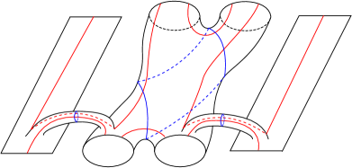
Figure 6. The bordered sutured Heegaard diagram for $\mathcal{P}$.

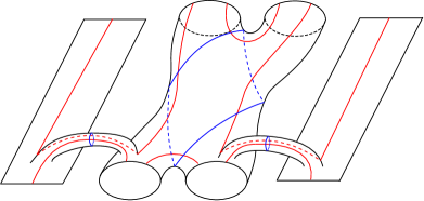
Figure 7. The bordered sutured Heegaard diagram for $\mathcal{N}$.

Remark 3.4.

The diagrams in Figure 6 and Figure 7 do not satisfy all the hypotheses necessary to be covered by Lipshitz–Ozsváth–Thurston’s results in [LOT15] or Zarev’s results in [Zar11]; Ozsváth–Szabó show in [OSz19a] that they can still be analyzed using a generalization of the analytic setup of bordered or bordered sutured Heegaard Floer homology. However, a more literal generalization of these theories would yield bimodules over the larger dg algebras of [LP20, MMW20] rather than over the associative algebra $\mathcal{B}(2)$. The second author, with Marengon and Willis, hope to address this difference in future work, defining $DA$ bimodules over the larger dg algebras and relating them to $\mathcal{P}$ and $\mathcal{N}$.

4. Higher representations

4.1. General setup

We now briefly review how higher representation theory interacts with bordered Heegaard Floer homology, as discussed in more generality in [MR20].

4.1.1. Monoidal category

The following differential monoidal category $\mathcal{U}$ was defined in [Kho14], and 2-actions of $\mathcal{U}$ are a main subject of [MR20] (see also [DM14, DLM19]).

Definition 4.1.

Let $\mathcal{U}$ denote the strict differential monoidal category with objects generated under $\otimes$ by a single object $e$ and with morphisms generated under $\otimes$ and composition by an endomorphism $\tau$ of $e\otimes e$, subject to the relations $\tau^{2}=0$ and

$$(\operatorname{id}_{e}\otimes\tau)\circ(\tau\otimes\operatorname{id}_{e})\circ(\operatorname{id}_{e}\otimes\tau)=(\tau\otimes\operatorname{id}_{e})\otimes(\operatorname{id}_{e}\otimes\tau)\otimes(\tau\otimes\operatorname{id}_{e}),$$

and with differential determined by $d(\tau)=\operatorname{id}_{e\otimes e}$.

Remark 4.2.

A grading on $\mathcal{U}$ is defined in [Kho14], making it into a dg category. Here we will not need to work with this grading; indeed, in the 2-actions of $\mathcal{U}$ we consider below, $\tau$ will act as zero.

The endomorphism algebra in $\mathcal{U}$ of $e^{\otimes m}$ is the nilCoxeter dg algebra denoted by $\mathfrak{N}_{m}$ in [DM14].

4.1.2. 2-representations

We will be especially concerned with 2-representations of $\mathcal{U}$ on associative algebras in the setting of $DA$ bimodules; we give a concrete definition of this notion below.

Definition 4.3.

Let $\mathcal{A}$ be an associative algebra (we make the same assumptions on $\mathcal{A}$ as in Section 2.1). A ($DA$ bimodule) 2-representation of $\mathcal{U}$ on $\mathcal{A}$ is the data of a $DA$ bimodule $\mathcal{E}$ over $\mathcal{A}$ and a (typically non-closed) $DA$ bimodule morphism $\tau$ from $\mathcal{E}\boxtimes\mathcal{E}$ to itself satisfying $\tau^{2}=0$,

$$(\operatorname{id}_{\mathcal{E}}\boxtimes\tau)\circ(\tau\boxtimes\operatorname{id}_{\mathcal{E}})\circ(\operatorname{id}_{\mathcal{E}}\boxtimes\tau)=(\tau\boxtimes\operatorname{id}_{\mathcal{E}})\circ(\operatorname{id}_{\mathcal{E}}\boxtimes\tau)\circ(\tau\boxtimes\operatorname{id}_{\mathcal{E}}),$$

and $d(\tau)=1$. We also assume that $\mathcal{E}$ is left bounded in the sense of [LOT15, Definition 2.2.46].

We will write the above data as $(\mathcal{A},\mathcal{E},\tau)$.

Remark 4.4.

The definitions of $DA$ bimodule morphisms, their tensor products, and their differentials can be found in [LOT15, Section 2.2.4 and Section 2.3.2], but we will refrain from spelling out these definitions here because in the examples we will consider, $\mathcal{E}\boxtimes\mathcal{E}$ will be the zero $DA$ bimodule and $\tau$ will be the zero morphism.

4.1.3. 1-morphisms of 2-representations

We will also work with a $DA$ bimodule version of 1-morphisms between 2-representations of $\mathcal{U}$.

Definition 4.5.

Let $(\mathcal{A},\mathcal{E},\tau)$ and $(\mathcal{A}^{\prime},\mathcal{E}^{\prime},\tau^{\prime})$ be ($DA$ bimodule) 2-representations of $\mathcal{U}$ on associative algebras $\mathcal{A}$ and $\mathcal{A}^{\prime}$. A ($DA$ bimodule) 1-morphism of 2-representations from $(\mathcal{A},\mathcal{E},\tau)$ to $(\mathcal{A}^{\prime},\mathcal{E}^{\prime},\tau^{\prime})$ consists of a left bounded $DA$ bimodule $X$ over $(\mathcal{A}^{\prime},\mathcal{A})$ together with a homotopy equivalence

$$\alpha\colon X\boxtimes\mathcal{E}\to\mathcal{E}^{\prime}\boxtimes X,$$

satisfying

$$(\tau^{\prime}\boxtimes\operatorname{id}_{X})\circ(\operatorname{id}_{\mathcal{E}^{\prime}}\boxtimes\alpha)\circ(\alpha\boxtimes\operatorname{id}_{\mathcal{E}})=(\operatorname{id}_{\mathcal{E}^{\prime}}\boxtimes\alpha)\circ(\alpha\boxtimes\operatorname{id}_{\mathcal{E}})\circ(\operatorname{id}_{X}\boxtimes\tau)$$

as morphisms from $X\boxtimes\mathcal{E}\boxtimes\mathcal{E}$ to $\mathcal{E}^{\prime}\boxtimes\mathcal{E}^{\prime}\boxtimes X$.

Remark 4.6.

We will not elaborate on the definition of homotopy equivalence of $DA$ bimodules here (it can be found in [LOT15, Section 2.2.4]); in this paper the homotopy equivalences $\alpha$ will be isomorphisms given by bijections between primary matrix entries such that the corresponding secondary matrices agree.

4.2. Actions on bordered HFK algebras

In [MR20], 2-representations of $\mathcal{U}$ are defined on the algebras $\mathcal{A}(\mathcal{Z})$ appearing in bordered sutured Heegaard Floer homology. Here $\mathcal{Z}$ denotes an arc diagram, i.e. a finite collection of oriented intervals and circles equipped with a 2-to-1 matching of finitely many points in the interiors of the intervals and circles, and there is a 2-representation of $\mathcal{U}$ on $\mathcal{A}(\mathcal{Z})$ for each interval in $\mathcal{Z}$.

The algebra $\mathcal{B}(2)$ was shown in [MMW20, LP20] to be quasi-isomorphic to $\mathcal{A}(\mathcal{Z})$ where $\mathcal{Z}$ is the arc diagram shown in Figure 8. Since $\mathcal{Z}$ has two intervals, we should expect two 2-actions of $\mathcal{U}$ on $\mathcal{B}(2)$; we define these 2-actions below. See [LM21] for a related 2-representation of $\mathcal{U}$ on an $n$-strand Ozsváth–Szabó algebra from [OSz18]. In more detail, we will define $DA$ bimodules $\mathcal{E}_{1}$ and $\mathcal{E}_{2}$ over $\mathcal{B}(2)$; these bimodules will satisfy $\mathcal{E}_{i}\boxtimes\mathcal{E}_{i}=0$, so that $(\mathcal{A},\mathcal{E}_{i},0)$ is a 2-representation of $\mathcal{U}$.

Remark 4.7.

The arc diagram shown in Figure 8 can also be seen on the front and back edges of the Heegaard diagrams in Figure 6 and Figure 7, with the red arcs in Figure 8 determined by the matching pattern of the red arcs in the Heegaard diagrams.

Figure 8. The arc diagram $\mathcal{Z}$ such that $\mathcal{A}(\mathcal{Z})$ is quasi-isomorphic to $\mathcal{B}(2)$; the 2-to-1 matching is indicated by the red arcs, and by symmetry one may take any orientation on the circles and intervals.

Definition 4.8.

The primary matrix for $\mathcal{E}_{1}$ has block form with the following blocks (we write e.g. $X_{1}$ for the singleton set $\{X_{1}\}$):

$$\hbox{}\vbox{\kern 0.86108pt\hbox{$\kern 0.0pt\kern 2.5pt\kern-5.0pt\left[\kern 0.0pt\kern-2.5pt\kern-5.55557pt\vbox{\kern-0.86108pt\vbox{\vbox{ \halign{\kern\arraycolsep\hfil\@arstrut$\kbcolstyle#$\hfil\kern\arraycolsep& \kern\arraycolsep\hfil$\@kbrowstyle#$\ifkbalignright\relax\else\hfil\fi\kern\arraycolsep&& \kern\arraycolsep\hfil$\@kbrowstyle#$\ifkbalignright\relax\else\hfil\fi\kern\arraycolsep\cr 5.0pt\hfil\@arstrut$\scriptstyle$\hfil\kern 5.0pt&5.0pt\hfil$\scriptstyle A$\hfil\kern 5.0pt&5.0pt\hfil$\scriptstyle B$\hfil\kern 5.0pt&5.0pt\hfil$\scriptstyle C\\\varnothing$\hfil\kern 5.0pt&5.0pt\hfil$\scriptstyle X_{1}$\hfil\kern 5.0pt&5.0pt\hfil$\scriptstyle\varnothing$\hfil\kern 5.0pt&5.0pt\hfil$\scriptstyle\varnothing$\hfil\kern 5.0pt\crcr}}}}\right]$}},\hbox{}\vbox{\kern 0.86108pt\hbox{$\kern 0.0pt\kern 2.5pt\kern-5.0pt\left[\kern 0.0pt\kern-2.5pt\kern-5.55557pt\vbox{\kern-0.86108pt\vbox{\vbox{ \halign{\kern\arraycolsep\hfil\@arstrut$\kbcolstyle#$\hfil\kern\arraycolsep& \kern\arraycolsep\hfil$\@kbrowstyle#$\ifkbalignright\relax\else\hfil\fi\kern\arraycolsep&& \kern\arraycolsep\hfil$\@kbrowstyle#$\ifkbalignright\relax\else\hfil\fi\kern\arraycolsep\cr 5.0pt\hfil\@arstrut$\scriptstyle$\hfil\kern 5.0pt&5.0pt\hfil$\scriptstyle AB$\hfil\kern 5.0pt&5.0pt\hfil$\scriptstyle AC$\hfil\kern 5.0pt&5.0pt\hfil$\scriptstyle BC\\A$\hfil\kern 5.0pt&5.0pt\hfil$\scriptstyle\varnothing$\hfil\kern 5.0pt&5.0pt\hfil$\scriptstyle\varnothing$\hfil\kern 5.0pt&5.0pt\hfil$\scriptstyle\varnothing\\B$\hfil\kern 5.0pt&5.0pt\hfil$\scriptstyle X_{2}$\hfil\kern 5.0pt&5.0pt\hfil$\scriptstyle\varnothing$\hfil\kern 5.0pt&5.0pt\hfil$\scriptstyle\varnothing\\C$\hfil\kern 5.0pt&5.0pt\hfil$\scriptstyle\varnothing$\hfil\kern 5.0pt&5.0pt\hfil$\scriptstyle X_{3}$\hfil\kern 5.0pt&5.0pt\hfil$\scriptstyle\varnothing$\hfil\kern 5.0pt\crcr}}}}\right]$}},\hbox{}\vbox{\kern 0.86108pt\hbox{$\kern 0.0pt\kern 2.5pt\kern-5.0pt\left[\kern 0.0pt\kern-2.5pt\kern-5.55557pt\vbox{\kern-0.86108pt\vbox{\vbox{ \halign{\kern\arraycolsep\hfil\@arstrut$\kbcolstyle#$\hfil\kern\arraycolsep& \kern\arraycolsep\hfil$\@kbrowstyle#$\ifkbalignright\relax\else\hfil\fi\kern\arraycolsep&& \kern\arraycolsep\hfil$\@kbrowstyle#$\ifkbalignright\relax\else\hfil\fi\kern\arraycolsep\cr 5.0pt\hfil\@arstrut$\scriptstyle$\hfil\kern 5.0pt&5.0pt\hfil$\scriptstyle ABC\\AB$\hfil\kern 5.0pt&5.0pt\hfil$\scriptstyle\varnothing\\AC$\hfil\kern 5.0pt&5.0pt\hfil$\scriptstyle\varnothing\\BC$\hfil\kern 5.0pt&5.0pt\hfil$\scriptstyle X_{4}$\hfil\kern 5.0pt\crcr}}}}\right]$}}.$$

The secondary matrix for $\mathcal{E}_{1}$ has a corresponding block form with blocks

$$\hbox{}\vbox{\kern 0.86108pt\hbox{$\kern 0.0pt\kern 2.5pt\kern-5.0pt\left[\kern 0.0pt\kern-2.5pt\kern-5.55557pt\vbox{\kern-0.86108pt\vbox{\vbox{ \halign{\kern\arraycolsep\hfil\@arstrut$\kbcolstyle#$\hfil\kern\arraycolsep& \kern\arraycolsep\hfil$\@kbrowstyle#$\ifkbalignright\relax\else\hfil\fi\kern\arraycolsep&& \kern\arraycolsep\hfil$\@kbrowstyle#$\ifkbalignright\relax\else\hfil\fi\kern\arraycolsep\cr 5.0pt\hfil\@arstrut$\scriptstyle$\hfil\kern 5.0pt&5.0pt\hfil$\scriptstyle X_{1}\\X_{1}$\hfil\kern 5.0pt&5.0pt\hfil$\scriptstyle 0$\hfil\kern 5.0pt\crcr}}}}\right]$}},$$

$$\hbox{}\vbox{\kern 0.86108pt\hbox{$\kern 0.0pt\kern 2.5pt\kern-5.0pt\left[\kern 0.0pt\kern-2.5pt\kern-5.55557pt\vbox{\kern-0.86108pt\vbox{\vbox{ \halign{\kern\arraycolsep\hfil\@arstrut$\kbcolstyle#$\hfil\kern\arraycolsep& \kern\arraycolsep\hfil$\@kbrowstyle#$\ifkbalignright\relax\else\hfil\fi\kern\arraycolsep&& \kern\arraycolsep\hfil$\@kbrowstyle#$\ifkbalignright\relax\else\hfil\fi\kern\arraycolsep\cr 5.0pt\hfil\@arstrut$\scriptstyle$\hfil\kern 5.0pt&5.0pt\hfil$\scriptstyle X_{2}$\hfil\kern 5.0pt&5.0pt\hfil$\scriptstyle X_{3}\\X_{2}$\hfil\kern 5.0pt&5.0pt\hfil$\scriptstyle U_{1}^{k+1}\otimes U_{1}^{k+1}+U_{2}^{k+1}\otimes U_{2}^{k+1}$\hfil\kern 5.0pt&5.0pt\hfil$\scriptstyle L_{2}U_{2}^{k}\otimes L_{2}U_{2}^{k}\\X_{3}$\hfil\kern 5.0pt&5.0pt\hfil$\scriptstyle R_{2}U_{2}^{k}\otimes R_{2}U_{2}^{k}$\hfil\kern 5.0pt&5.0pt\hfil$\scriptstyle U_{2}^{k+1}\otimes U_{2}^{k+1}$\hfil\kern 5.0pt\crcr}}}}\right]$}},$$

$$\hbox{}\vbox{\kern 0.86108pt\hbox{$\kern 0.0pt\kern 2.5pt\kern-5.0pt\left[\kern 0.0pt\kern-2.5pt\kern-5.55557pt\vbox{\kern-0.86108pt\vbox{\vbox{ \halign{\kern\arraycolsep\hfil\@arstrut$\kbcolstyle#$\hfil\kern\arraycolsep& \kern\arraycolsep\hfil$\@kbrowstyle#$\ifkbalignright\relax\else\hfil\fi\kern\arraycolsep&& \kern\arraycolsep\hfil$\@kbrowstyle#$\ifkbalignright\relax\else\hfil\fi\kern\arraycolsep\cr 5.0pt\hfil\@arstrut$\scriptstyle$\hfil\kern 5.0pt&5.0pt\hfil$\scriptstyle X_{4}\\X_{4}$\hfil\kern 5.0pt&5.0pt\hfil$\scriptstyle U_{1}^{k}U_{2}^{l}\otimes U_{1}^{k}U_{2}^{l}$\hfil\kern 5.0pt\crcr}}}}\right]$}};$$

in the final block we disallow $(k,l)=(0,0)$ to match Convention 2.10.

Definition 4.9.

The primary matrix for $\mathcal{E}_{2}$ has block form with the following blocks (again we write e.g. $Y_{1}$ for the singleton set $\{Y_{1}\}$):

$$\hbox{}\vbox{\kern 0.86108pt\hbox{$\kern 0.0pt\kern 2.5pt\kern-5.0pt\left[\kern 0.0pt\kern-2.5pt\kern-5.55557pt\vbox{\kern-0.86108pt\vbox{\vbox{ \halign{\kern\arraycolsep\hfil\@arstrut$\kbcolstyle#$\hfil\kern\arraycolsep& \kern\arraycolsep\hfil$\@kbrowstyle#$\ifkbalignright\relax\else\hfil\fi\kern\arraycolsep&& \kern\arraycolsep\hfil$\@kbrowstyle#$\ifkbalignright\relax\else\hfil\fi\kern\arraycolsep\cr 5.0pt\hfil\@arstrut$\scriptstyle$\hfil\kern 5.0pt&5.0pt\hfil$\scriptstyle A$\hfil\kern 5.0pt&5.0pt\hfil$\scriptstyle B$\hfil\kern 5.0pt&5.0pt\hfil$\scriptstyle C\\\varnothing$\hfil\kern 5.0pt&5.0pt\hfil$\scriptstyle\varnothing$\hfil\kern 5.0pt&5.0pt\hfil$\scriptstyle\varnothing$\hfil\kern 5.0pt&5.0pt\hfil$\scriptstyle Y_{1}$\hfil\kern 5.0pt\crcr}}}}\right]$}},\hbox{}\vbox{\kern 0.86108pt\hbox{$\kern 0.0pt\kern 2.5pt\kern-5.0pt\left[\kern 0.0pt\kern-2.5pt\kern-5.55557pt\vbox{\kern-0.86108pt\vbox{\vbox{ \halign{\kern\arraycolsep\hfil\@arstrut$\kbcolstyle#$\hfil\kern\arraycolsep& \kern\arraycolsep\hfil$\@kbrowstyle#$\ifkbalignright\relax\else\hfil\fi\kern\arraycolsep&& \kern\arraycolsep\hfil$\@kbrowstyle#$\ifkbalignright\relax\else\hfil\fi\kern\arraycolsep\cr 5.0pt\hfil\@arstrut$\scriptstyle$\hfil\kern 5.0pt&5.0pt\hfil$\scriptstyle AB$\hfil\kern 5.0pt&5.0pt\hfil$\scriptstyle AC$\hfil\kern 5.0pt&5.0pt\hfil$\scriptstyle BC\\A$\hfil\kern 5.0pt&5.0pt\hfil$\scriptstyle\varnothing$\hfil\kern 5.0pt&5.0pt\hfil$\scriptstyle Y_{2}$\hfil\kern 5.0pt&5.0pt\hfil$\scriptstyle\varnothing\\B$\hfil\kern 5.0pt&5.0pt\hfil$\scriptstyle\varnothing$\hfil\kern 5.0pt&5.0pt\hfil$\scriptstyle\varnothing$\hfil\kern 5.0pt&5.0pt\hfil$\scriptstyle Y_{3}\\C$\hfil\kern 5.0pt&5.0pt\hfil$\scriptstyle\varnothing$\hfil\kern 5.0pt&5.0pt\hfil$\scriptstyle\varnothing$\hfil\kern 5.0pt&5.0pt\hfil$\scriptstyle\varnothing$\hfil\kern 5.0pt\crcr}}}}\right]$}},\hbox{}\vbox{\kern 0.86108pt\hbox{$\kern 0.0pt\kern 2.5pt\kern-5.0pt\left[\kern 0.0pt\kern-2.5pt\kern-5.55557pt\vbox{\kern-0.86108pt\vbox{\vbox{ \halign{\kern\arraycolsep\hfil\@arstrut$\kbcolstyle#$\hfil\kern\arraycolsep& \kern\arraycolsep\hfil$\@kbrowstyle#$\ifkbalignright\relax\else\hfil\fi\kern\arraycolsep&& \kern\arraycolsep\hfil$\@kbrowstyle#$\ifkbalignright\relax\else\hfil\fi\kern\arraycolsep\cr 5.0pt\hfil\@arstrut$\scriptstyle$\hfil\kern 5.0pt&5.0pt\hfil$\scriptstyle ABC\\AB$\hfil\kern 5.0pt&5.0pt\hfil$\scriptstyle Y_{4}\\AC$\hfil\kern 5.0pt&5.0pt\hfil$\scriptstyle\varnothing\\BC$\hfil\kern 5.0pt&5.0pt\hfil$\scriptstyle\varnothing$\hfil\kern 5.0pt\crcr}}}}\right]$}}.$$

The secondary matrix for $\mathcal{E}_{2}$ has a corresponding block form with blocks

$$\hbox{}\vbox{\kern 0.86108pt\hbox{$\kern 0.0pt\kern 2.5pt\kern-5.0pt\left[\kern 0.0pt\kern-2.5pt\kern-5.55557pt\vbox{\kern-0.86108pt\vbox{\vbox{ \halign{\kern\arraycolsep\hfil\@arstrut$\kbcolstyle#$\hfil\kern\arraycolsep& \kern\arraycolsep\hfil$\@kbrowstyle#$\ifkbalignright\relax\else\hfil\fi\kern\arraycolsep&& \kern\arraycolsep\hfil$\@kbrowstyle#$\ifkbalignright\relax\else\hfil\fi\kern\arraycolsep\cr 5.0pt\hfil\@arstrut$\scriptstyle$\hfil\kern 5.0pt&5.0pt\hfil$\scriptstyle Y_{1}\\Y_{1}$\hfil\kern 5.0pt&5.0pt\hfil$\scriptstyle 0$\hfil\kern 5.0pt\crcr}}}}\right]$}},$$

$$\hbox{}\vbox{\kern 0.86108pt\hbox{$\kern 0.0pt\kern 2.5pt\kern-5.0pt\left[\kern 0.0pt\kern-2.5pt\kern-5.55557pt\vbox{\kern-0.86108pt\vbox{\vbox{ \halign{\kern\arraycolsep\hfil\@arstrut$\kbcolstyle#$\hfil\kern\arraycolsep& \kern\arraycolsep\hfil$\@kbrowstyle#$\ifkbalignright\relax\else\hfil\fi\kern\arraycolsep&& \kern\arraycolsep\hfil$\@kbrowstyle#$\ifkbalignright\relax\else\hfil\fi\kern\arraycolsep\cr 5.0pt\hfil\@arstrut$\scriptstyle$\hfil\kern 5.0pt&5.0pt\hfil$\scriptstyle Y_{2}$\hfil\kern 5.0pt&5.0pt\hfil$\scriptstyle Y_{3}\\Y_{2}$\hfil\kern 5.0pt&5.0pt\hfil$\scriptstyle U_{1}^{k+1}\otimes U_{1}^{k+1}$\hfil\kern 5.0pt&5.0pt\hfil$\scriptstyle L_{1}U_{1}^{k}\otimes L_{1}U_{1}^{k}\\Y_{3}$\hfil\kern 5.0pt&5.0pt\hfil$\scriptstyle R_{1}U_{1}^{k}\otimes R_{1}U_{1}^{k}$\hfil\kern 5.0pt&5.0pt\hfil$\scriptstyle U_{1}^{k+1}\otimes U_{1}^{k+1}+U_{2}^{k+1}\otimes U_{2}^{k+1}$\hfil\kern 5.0pt\crcr}}}}\right]$}},$$

$$\hbox{}\vbox{\kern 0.86108pt\hbox{$\kern 0.0pt\kern 2.5pt\kern-5.0pt\left[\kern 0.0pt\kern-2.5pt\kern-5.55557pt\vbox{\kern-0.86108pt\vbox{\vbox{ \halign{\kern\arraycolsep\hfil\@arstrut$\kbcolstyle#$\hfil\kern\arraycolsep& \kern\arraycolsep\hfil$\@kbrowstyle#$\ifkbalignright\relax\else\hfil\fi\kern\arraycolsep&& \kern\arraycolsep\hfil$\@kbrowstyle#$\ifkbalignright\relax\else\hfil\fi\kern\arraycolsep\cr 5.0pt\hfil\@arstrut$\scriptstyle$\hfil\kern 5.0pt&5.0pt\hfil$\scriptstyle Y_{4}\\Y_{4}$\hfil\kern 5.0pt&5.0pt\hfil$\scriptstyle U_{1}^{k}U_{2}^{l}\otimes U_{1}U_{2}^{l}$\hfil\kern 5.0pt\crcr}}}}\right]$}};$$

in the final block we disallow $(k,l)=(0,0)$ to match Convention 2.10.

By multiplying the primary matrix for $\mathcal{E}_{i}$ by itself ($i=1,2$), one can see that $\mathcal{E}_{i}\boxtimes\mathcal{E}_{i}$ has a primary matrix with each entry the empty set; in other words, $\mathcal{E}_{i}\boxtimes\mathcal{E}_{i}$ is zero as claimed above.

5. 1-morphism structure for $\mathcal{P}$

5.1. Commutativity with $\mathcal{E}_{1}$

5.1.1. The bimodule $\mathcal{E}_{1}\boxtimes\mathcal{P}$

We give a matrix description for $\mathcal{E}_{1}\boxtimes\mathcal{P}$ following Section 2.4. To get the primary matrix for $\mathcal{E}_{1}\boxtimes\mathcal{P}$, we multiply the primary matrices for $\mathcal{E}_{1}$ and $\mathcal{P}$. We can do this block-by-block, so the primary matrix for $\mathcal{E}_{1}\boxtimes\mathcal{P}$ has block form with blocks given by

$$\hbox{}\vbox{\kern 0.86108pt\hbox{$\kern 0.0pt\kern 2.5pt\kern-5.0pt\left[\kern 0.0pt\kern-2.5pt\kern-5.55557pt\vbox{\kern-0.86108pt\vbox{\vbox{ \halign{\kern\arraycolsep\hfil\@arstrut$\kbcolstyle#$\hfil\kern\arraycolsep& \kern\arraycolsep\hfil$\@kbrowstyle#$\ifkbalignright\relax\else\hfil\fi\kern\arraycolsep&& \kern\arraycolsep\hfil$\@kbrowstyle#$\ifkbalignright\relax\else\hfil\fi\kern\arraycolsep\cr 5.0pt\hfil\@arstrut$\scriptstyle$\hfil\kern 5.0pt&5.0pt\hfil$\scriptstyle A$\hfil\kern 5.0pt&5.0pt\hfil$\scriptstyle B$\hfil\kern 5.0pt&5.0pt\hfil$\scriptstyle C\\\varnothing$\hfil\kern 5.0pt&5.0pt\hfil$\scriptstyle X_{1}$\hfil\kern 5.0pt&5.0pt\hfil$\scriptstyle\varnothing$\hfil\kern 5.0pt&5.0pt\hfil$\scriptstyle\varnothing$\hfil\kern 5.0pt\crcr}}}}\right]$}}\cdot\hbox{}\vbox{\kern 0.86108pt\hbox{$\kern 0.0pt\kern 2.5pt\kern-5.0pt\left[\kern 0.0pt\kern-2.5pt\kern-5.55557pt\vbox{\kern-0.86108pt\vbox{\vbox{ \halign{\kern\arraycolsep\hfil\@arstrut$\kbcolstyle#$\hfil\kern\arraycolsep& \kern\arraycolsep\hfil$\@kbrowstyle#$\ifkbalignright\relax\else\hfil\fi\kern\arraycolsep&& \kern\arraycolsep\hfil$\@kbrowstyle#$\ifkbalignright\relax\else\hfil\fi\kern\arraycolsep\cr 5.0pt\hfil\@arstrut$\scriptstyle$\hfil\kern 5.0pt&5.0pt\hfil$\scriptstyle A$\hfil\kern 5.0pt&5.0pt\hfil$\scriptstyle B$\hfil\kern 5.0pt&5.0pt\hfil$\scriptstyle C\\A$\hfil\kern 5.0pt&5.0pt\hfil$\scriptstyle S_{A}$\hfil\kern 5.0pt&5.0pt\hfil$\scriptstyle\varnothing$\hfil\kern 5.0pt&5.0pt\hfil$\scriptstyle\varnothing\\B$\hfil\kern 5.0pt&5.0pt\hfil$\scriptstyle W$\hfil\kern 5.0pt&5.0pt\hfil$\scriptstyle N$\hfil\kern 5.0pt&5.0pt\hfil$\scriptstyle E\\C$\hfil\kern 5.0pt&5.0pt\hfil$\scriptstyle\varnothing$\hfil\kern 5.0pt&5.0pt\hfil$\scriptstyle\varnothing$\hfil\kern 5.0pt&5.0pt\hfil$\scriptstyle S_{C}$\hfil\kern 5.0pt\crcr}}}}\right]$}}=\hbox{}\vbox{\kern 0.86108pt\hbox{$\kern 0.0pt\kern 2.5pt\kern-5.0pt\left[\kern 0.0pt\kern-2.5pt\kern-5.55557pt\vbox{\kern-0.86108pt\vbox{\vbox{ \halign{\kern\arraycolsep\hfil\@arstrut$\kbcolstyle#$\hfil\kern\arraycolsep& \kern\arraycolsep\hfil$\@kbrowstyle#$\ifkbalignright\relax\else\hfil\fi\kern\arraycolsep&& \kern\arraycolsep\hfil$\@kbrowstyle#$\ifkbalignright\relax\else\hfil\fi\kern\arraycolsep\cr 5.0pt\hfil\@arstrut$\scriptstyle$\hfil\kern 5.0pt&5.0pt\hfil$\scriptstyle A$\hfil\kern 5.0pt&5.0pt\hfil$\scriptstyle B$\hfil\kern 5.0pt&5.0pt\hfil$\scriptstyle C\\\varnothing$\hfil\kern 5.0pt&5.0pt\hfil$\scriptstyle X_{1}S_{C}$\hfil\kern 5.0pt&5.0pt\hfil$\scriptstyle\varnothing$\hfil\kern 5.0pt&5.0pt\hfil$\scriptstyle\varnothing$\hfil\kern 5.0pt\crcr}}}}\right]$}},$$

$$\hbox{}\vbox{\kern 0.86108pt\hbox{$\kern 0.0pt\kern 2.5pt\kern-5.0pt\left[\kern 0.0pt\kern-2.5pt\kern-5.55557pt\vbox{\kern-0.86108pt\vbox{\vbox{ \halign{\kern\arraycolsep\hfil\@arstrut$\kbcolstyle#$\hfil\kern\arraycolsep& \kern\arraycolsep\hfil$\@kbrowstyle#$\ifkbalignright\relax\else\hfil\fi\kern\arraycolsep&& \kern\arraycolsep\hfil$\@kbrowstyle#$\ifkbalignright\relax\else\hfil\fi\kern\arraycolsep\cr 5.0pt\hfil\@arstrut$\scriptstyle$\hfil\kern 5.0pt&5.0pt\hfil$\scriptstyle AB$\hfil\kern 5.0pt&5.0pt\hfil$\scriptstyle AC$\hfil\kern 5.0pt&5.0pt\hfil$\scriptstyle BC\\A$\hfil\kern 5.0pt&5.0pt\hfil$\scriptstyle\varnothing$\hfil\kern 5.0pt&5.0pt\hfil$\scriptstyle\varnothing$\hfil\kern 5.0pt&5.0pt\hfil$\scriptstyle\varnothing\\B$\hfil\kern 5.0pt&5.0pt\hfil$\scriptstyle X_{2}$\hfil\kern 5.0pt&5.0pt\hfil$\scriptstyle\varnothing$\hfil\kern 5.0pt&5.0pt\hfil$\scriptstyle\varnothing\\C$\hfil\kern 5.0pt&5.0pt\hfil$\scriptstyle\varnothing$\hfil\kern 5.0pt&5.0pt\hfil$\scriptstyle X_{3}$\hfil\kern 5.0pt&5.0pt\hfil$\scriptstyle\varnothing$\hfil\kern 5.0pt\crcr}}}}\right]$}}\cdot\hbox{}\vbox{\kern 0.86108pt\hbox{$\kern 0.0pt\kern 2.5pt\kern-5.0pt\left[\kern 0.0pt\kern-2.5pt\kern-5.55557pt\vbox{\kern-0.86108pt\vbox{\vbox{ \halign{\kern\arraycolsep\hfil\@arstrut$\kbcolstyle#$\hfil\kern\arraycolsep& \kern\arraycolsep\hfil$\@kbrowstyle#$\ifkbalignright\relax\else\hfil\fi\kern\arraycolsep&& \kern\arraycolsep\hfil$\@kbrowstyle#$\ifkbalignright\relax\else\hfil\fi\kern\arraycolsep\cr 5.0pt\hfil\@arstrut$\scriptstyle$\hfil\kern 5.0pt&5.0pt\hfil$\scriptstyle AB$\hfil\kern 5.0pt&5.0pt\hfil$\scriptstyle AC$\hfil\kern 5.0pt&5.0pt\hfil$\scriptstyle BC\\AB$\hfil\kern 5.0pt&5.0pt\hfil$\scriptstyle N_{AB}$\hfil\kern 5.0pt&5.0pt\hfil$\scriptstyle E$\hfil\kern 5.0pt&5.0pt\hfil$\scriptstyle\varnothing\\AC$\hfil\kern 5.0pt&5.0pt\hfil$\scriptstyle\varnothing$\hfil\kern 5.0pt&5.0pt\hfil$\scriptstyle S$\hfil\kern 5.0pt&5.0pt\hfil$\scriptstyle\varnothing\\BC$\hfil\kern 5.0pt&5.0pt\hfil$\scriptstyle\varnothing$\hfil\kern 5.0pt&5.0pt\hfil$\scriptstyle W$\hfil\kern 5.0pt&5.0pt\hfil$\scriptstyle N_{BC}$\hfil\kern 5.0pt\crcr}}}}\right]$}}=\hbox{}\vbox{\kern 0.86108pt\hbox{$\kern 0.0pt\kern 2.5pt\kern-5.0pt\left[\kern 0.0pt\kern-2.5pt\kern-5.55557pt\vbox{\kern-0.86108pt\vbox{\vbox{ \halign{\kern\arraycolsep\hfil\@arstrut$\kbcolstyle#$\hfil\kern\arraycolsep& \kern\arraycolsep\hfil$\@kbrowstyle#$\ifkbalignright\relax\else\hfil\fi\kern\arraycolsep&& \kern\arraycolsep\hfil$\@kbrowstyle#$\ifkbalignright\relax\else\hfil\fi\kern\arraycolsep\cr 5.0pt\hfil\@arstrut$\scriptstyle$\hfil\kern 5.0pt&5.0pt\hfil$\scriptstyle AB$\hfil\kern 5.0pt&5.0pt\hfil$\scriptstyle AC$\hfil\kern 5.0pt&5.0pt\hfil$\scriptstyle BC\\A$\hfil\kern 5.0pt&5.0pt\hfil$\scriptstyle\varnothing$\hfil\kern 5.0pt&5.0pt\hfil$\scriptstyle\varnothing$\hfil\kern 5.0pt&5.0pt\hfil$\scriptstyle\varnothing\\B$\hfil\kern 5.0pt&5.0pt\hfil$\scriptstyle X_{2}N_{AB}$\hfil\kern 5.0pt&5.0pt\hfil$\scriptstyle X_{2}E$\hfil\kern 5.0pt&5.0pt\hfil$\scriptstyle\varnothing\\C$\hfil\kern 5.0pt&5.0pt\hfil$\scriptstyle\varnothing$\hfil\kern 5.0pt&5.0pt\hfil$\scriptstyle X_{3}X$\hfil\kern 5.0pt&5.0pt\hfil$\scriptstyle\varnothing$\hfil\kern 5.0pt\crcr}}}}\right]$}},$$

$$\hbox{}\vbox{\kern 0.86108pt\hbox{$\kern 0.0pt\kern 2.5pt\kern-5.0pt\left[\kern 0.0pt\kern-2.5pt\kern-5.55557pt\vbox{\kern-0.86108pt\vbox{\vbox{ \halign{\kern\arraycolsep\hfil\@arstrut$\kbcolstyle#$\hfil\kern\arraycolsep& \kern\arraycolsep\hfil$\@kbrowstyle#$\ifkbalignright\relax\else\hfil\fi\kern\arraycolsep&& \kern\arraycolsep\hfil$\@kbrowstyle#$\ifkbalignright\relax\else\hfil\fi\kern\arraycolsep\cr 5.0pt\hfil\@arstrut$\scriptstyle$\hfil\kern 5.0pt&5.0pt\hfil$\scriptstyle ABC\\AB$\hfil\kern 5.0pt&5.0pt\hfil$\scriptstyle\varnothing\\AC$\hfil\kern 5.0pt&5.0pt\hfil$\scriptstyle\varnothing\\BC$\hfil\kern 5.0pt&5.0pt\hfil$\scriptstyle X_{4}$\hfil\kern 5.0pt\crcr}}}}\right]$}}\cdot\hbox{}\vbox{\kern 0.86108pt\hbox{$\kern 0.0pt\kern 2.5pt\kern-5.0pt\left[\kern 0.0pt\kern-2.5pt\kern-5.55557pt\vbox{\kern-0.86108pt\vbox{\vbox{ \halign{\kern\arraycolsep\hfil\@arstrut$\kbcolstyle#$\hfil\kern\arraycolsep& \kern\arraycolsep\hfil$\@kbrowstyle#$\ifkbalignright\relax\else\hfil\fi\kern\arraycolsep&& \kern\arraycolsep\hfil$\@kbrowstyle#$\ifkbalignright\relax\else\hfil\fi\kern\arraycolsep\cr 5.0pt\hfil\@arstrut$\scriptstyle$\hfil\kern 5.0pt&5.0pt\hfil$\scriptstyle ABC\\ABC$\hfil\kern 5.0pt&5.0pt\hfil$\scriptstyle N$\hfil\kern 5.0pt\crcr}}}}\right]$}}=\hbox{}\vbox{\kern 0.86108pt\hbox{$\kern 0.0pt\kern 2.5pt\kern-5.0pt\left[\kern 0.0pt\kern-2.5pt\kern-5.55557pt\vbox{\kern-0.86108pt\vbox{\vbox{ \halign{\kern\arraycolsep\hfil\@arstrut$\kbcolstyle#$\hfil\kern\arraycolsep& \kern\arraycolsep\hfil$\@kbrowstyle#$\ifkbalignright\relax\else\hfil\fi\kern\arraycolsep&& \kern\arraycolsep\hfil$\@kbrowstyle#$\ifkbalignright\relax\else\hfil\fi\kern\arraycolsep\cr 5.0pt\hfil\@arstrut$\scriptstyle$\hfil\kern 5.0pt&5.0pt\hfil$\scriptstyle ABC\\AB$\hfil\kern 5.0pt&5.0pt\hfil$\scriptstyle\varnothing\\AC$\hfil\kern 5.0pt&5.0pt\hfil$\scriptstyle\varnothing\\BC$\hfil\kern 5.0pt&5.0pt\hfil$\scriptstyle X_{4}N$\hfil\kern 5.0pt\crcr}}}}\right]$}}.$$

In these matrices, we indicate idempotents only when necessary to distinguish primary matrix entries in the same block (so, for example, in the block with rows and columns $A,B,C$, we distinguish between two types of $S$ generators, but the only $N$ generator in this block is ${{}_{B}}N_{B}$ so we omit the idempotents and just write $N$).

The secondary matrix for $\mathcal{E}_{1}\boxtimes\mathcal{P}$ also has block form with blocks given by

$$\hbox{}\vbox{\kern 0.86108pt\hbox{$\kern 0.0pt\kern 2.5pt\kern-5.0pt\left[\kern 0.0pt\kern-2.5pt\kern-5.55557pt\vbox{\kern-0.86108pt\vbox{\vbox{ \halign{\kern\arraycolsep\hfil\@arstrut$\kbcolstyle#$\hfil\kern\arraycolsep& \kern\arraycolsep\hfil$\@kbrowstyle#$\ifkbalignright\relax\else\hfil\fi\kern\arraycolsep&& \kern\arraycolsep\hfil$\@kbrowstyle#$\ifkbalignright\relax\else\hfil\fi\kern\arraycolsep\cr 5.0pt\hfil\@arstrut$\scriptstyle$\hfil\kern 5.0pt&5.0pt\hfil$\scriptstyle X_{1}S_{C}\\X_{1}S_{C}$\hfil\kern 5.0pt&5.0pt\hfil$\scriptstyle 0$\hfil\kern 5.0pt\crcr}}}}\right]$}},$$

$$\hbox{}\vbox{\kern 0.86108pt\hbox{$\kern 0.0pt\kern 2.5pt\kern-5.0pt\left[\kern 0.0pt\kern-2.5pt\kern-5.55557pt\vbox{\kern-0.86108pt\vbox{\vbox{ \halign{\kern\arraycolsep\hfil\@arstrut$\kbcolstyle#$\hfil\kern\arraycolsep& \kern\arraycolsep\hfil$\@kbrowstyle#$\ifkbalignright\relax\else\hfil\fi\kern\arraycolsep&& \kern\arraycolsep\hfil$\@kbrowstyle#$\ifkbalignright\relax\else\hfil\fi\kern\arraycolsep\cr 5.0pt\hfil\@arstrut$\scriptstyle$\hfil\kern 5.0pt&5.0pt\hfil$\scriptstyle X_{2}N_{AB}$\hfil\kern 5.0pt&5.0pt\hfil$\scriptstyle X_{2}E$\hfil\kern 5.0pt&5.0pt\hfil$\scriptstyle X_{3}S\\X_{2}N_{AB}$\hfil\kern 5.0pt&5.0pt\hfil$\scriptstyle U_{2}^{k+1}\otimes U_{1}^{k+1}+U_{1}^{k+1}\otimes U_{2}^{k+1}$\hfil\kern 5.0pt&5.0pt\hfil$\scriptstyle U_{1}^{k}\otimes L_{2}U_{2}^{k}$\hfil\kern 5.0pt&5.0pt\hfil$\scriptstyle L_{2}U_{2}^{k}\otimes(L_{2},U_{1}^{k+1})\\X_{2}E$\hfil\kern 5.0pt&5.0pt\hfil$\scriptstyle U_{1}^{k+1}\otimes R_{2}U_{2}^{k}$\hfil\kern 5.0pt&5.0pt\hfil$\scriptstyle U_{1}^{k+1}\otimes U_{2}^{k+1}$\hfil\kern 5.0pt&5.0pt\hfil$\scriptstyle 0\\X_{3}S$\hfil\kern 5.0pt&5.0pt\hfil$\scriptstyle 0$\hfil\kern 5.0pt&5.0pt\hfil$\scriptstyle R_{2}$\hfil\kern 5.0pt&5.0pt\hfil$\scriptstyle 0$\hfil\kern 5.0pt\crcr}}}}\right]$}},$$

$$\hbox{}\vbox{\kern 0.86108pt\hbox{$\kern 0.0pt\kern 2.5pt\kern-5.0pt\left[\kern 0.0pt\kern-2.5pt\kern-5.55557pt\vbox{\kern-0.86108pt\vbox{\vbox{ \halign{\kern\arraycolsep\hfil\@arstrut$\kbcolstyle#$\hfil\kern\arraycolsep& \kern\arraycolsep\hfil$\@kbrowstyle#$\ifkbalignright\relax\else\hfil\fi\kern\arraycolsep&& \kern\arraycolsep\hfil$\@kbrowstyle#$\ifkbalignright\relax\else\hfil\fi\kern\arraycolsep\cr 5.0pt\hfil\@arstrut$\scriptstyle$\hfil\kern 5.0pt&5.0pt\hfil$\scriptstyle X_{4}N\\X_{4}N$\hfil\kern 5.0pt&5.0pt\hfil$\scriptstyle U_{1}^{l}U_{2}^{k}\otimes U_{1}^{k}U_{2}^{l}$\hfil\kern 5.0pt\crcr}}}}\right]$}};$$

in the final block we disallow $(k,l)=(0,0)$. An explanation for the terms in the secondary matrix is given in Figure 9, which uses the operation graph depictions of Figure 3.

Figure 9. Operation graphs for the terms in the secondary matrix of $\mathcal{E}_{1}\boxtimes\mathcal{P}$.

5.1.2. The bimodule $\mathcal{P}\boxtimes\mathcal{E}_{1}$

Similarly, we give a matrix description for $\mathcal{P}\boxtimes\mathcal{E}_{1}$. The primary matrix has block form with blocks

$$\hbox{}\vbox{\kern 0.86108pt\hbox{$\kern 0.0pt\kern 2.5pt\kern-5.0pt\left[\kern 0.0pt\kern-2.5pt\kern-5.55557pt\vbox{\kern-0.86108pt\vbox{\vbox{ \halign{\kern\arraycolsep\hfil\@arstrut$\kbcolstyle#$\hfil\kern\arraycolsep& \kern\arraycolsep\hfil$\@kbrowstyle#$\ifkbalignright\relax\else\hfil\fi\kern\arraycolsep&& \kern\arraycolsep\hfil$\@kbrowstyle#$\ifkbalignright\relax\else\hfil\fi\kern\arraycolsep\cr 5.0pt\hfil\@arstrut$\scriptstyle$\hfil\kern 5.0pt&5.0pt\hfil$\scriptstyle\varnothing\\\varnothing$\hfil\kern 5.0pt&5.0pt\hfil$\scriptstyle S$\hfil\kern 5.0pt\crcr}}}}\right]$}}\cdot\hbox{}\vbox{\kern 0.86108pt\hbox{$\kern 0.0pt\kern 2.5pt\kern-5.0pt\left[\kern 0.0pt\kern-2.5pt\kern-5.55557pt\vbox{\kern-0.86108pt\vbox{\vbox{ \halign{\kern\arraycolsep\hfil\@arstrut$\kbcolstyle#$\hfil\kern\arraycolsep& \kern\arraycolsep\hfil$\@kbrowstyle#$\ifkbalignright\relax\else\hfil\fi\kern\arraycolsep&& \kern\arraycolsep\hfil$\@kbrowstyle#$\ifkbalignright\relax\else\hfil\fi\kern\arraycolsep\cr 5.0pt\hfil\@arstrut$\scriptstyle$\hfil\kern 5.0pt&5.0pt\hfil$\scriptstyle A$\hfil\kern 5.0pt&5.0pt\hfil$\scriptstyle B$\hfil\kern 5.0pt&5.0pt\hfil$\scriptstyle C\\\varnothing$\hfil\kern 5.0pt&5.0pt\hfil$\scriptstyle X_{1}$\hfil\kern 5.0pt&5.0pt\hfil$\scriptstyle\varnothing$\hfil\kern 5.0pt&5.0pt\hfil$\scriptstyle\varnothing$\hfil\kern 5.0pt\crcr}}}}\right]$}}=\hbox{}\vbox{\kern 0.86108pt\hbox{$\kern 0.0pt\kern 2.5pt\kern-5.0pt\left[\kern 0.0pt\kern-2.5pt\kern-5.55557pt\vbox{\kern-0.86108pt\vbox{\vbox{ \halign{\kern\arraycolsep\hfil\@arstrut$\kbcolstyle#$\hfil\kern\arraycolsep& \kern\arraycolsep\hfil$\@kbrowstyle#$\ifkbalignright\relax\else\hfil\fi\kern\arraycolsep&& \kern\arraycolsep\hfil$\@kbrowstyle#$\ifkbalignright\relax\else\hfil\fi\kern\arraycolsep\cr 5.0pt\hfil\@arstrut$\scriptstyle$\hfil\kern 5.0pt&5.0pt\hfil$\scriptstyle A$\hfil\kern 5.0pt&5.0pt\hfil$\scriptstyle B$\hfil\kern 5.0pt&5.0pt\hfil$\scriptstyle C\\\varnothing$\hfil\kern 5.0pt&5.0pt\hfil$\scriptstyle SX_{1}$\hfil\kern 5.0pt&5.0pt\hfil$\scriptstyle\varnothing$\hfil\kern 5.0pt&5.0pt\hfil$\scriptstyle\varnothing$\hfil\kern 5.0pt\crcr}}}}\right]$}},$$

$$\hbox{}\vbox{\kern 0.86108pt\hbox{$\kern 0.0pt\kern 2.5pt\kern-5.0pt\left[\kern 0.0pt\kern-2.5pt\kern-5.55557pt\vbox{\kern-0.86108pt\vbox{\vbox{ \halign{\kern\arraycolsep\hfil\@arstrut$\kbcolstyle#$\hfil\kern\arraycolsep& \kern\arraycolsep\hfil$\@kbrowstyle#$\ifkbalignright\relax\else\hfil\fi\kern\arraycolsep&& \kern\arraycolsep\hfil$\@kbrowstyle#$\ifkbalignright\relax\else\hfil\fi\kern\arraycolsep\cr 5.0pt\hfil\@arstrut$\scriptstyle$\hfil\kern 5.0pt&5.0pt\hfil$\scriptstyle A$\hfil\kern 5.0pt&5.0pt\hfil$\scriptstyle B$\hfil\kern 5.0pt&5.0pt\hfil$\scriptstyle C\\A$\hfil\kern 5.0pt&5.0pt\hfil$\scriptstyle S_{A}$\hfil\kern 5.0pt&5.0pt\hfil$\scriptstyle\varnothing$\hfil\kern 5.0pt&5.0pt\hfil$\scriptstyle\varnothing\\B$\hfil\kern 5.0pt&5.0pt\hfil$\scriptstyle W$\hfil\kern 5.0pt&5.0pt\hfil$\scriptstyle N$\hfil\kern 5.0pt&5.0pt\hfil$\scriptstyle E\\C$\hfil\kern 5.0pt&5.0pt\hfil$\scriptstyle\varnothing$\hfil\kern 5.0pt&5.0pt\hfil$\scriptstyle\varnothing$\hfil\kern 5.0pt&5.0pt\hfil$\scriptstyle S_{C}$\hfil\kern 5.0pt\crcr}}}}\right]$}}\cdot\hbox{}\vbox{\kern 0.86108pt\hbox{$\kern 0.0pt\kern 2.5pt\kern-5.0pt\left[\kern 0.0pt\kern-2.5pt\kern-5.55557pt\vbox{\kern-0.86108pt\vbox{\vbox{ \halign{\kern\arraycolsep\hfil\@arstrut$\kbcolstyle#$\hfil\kern\arraycolsep& \kern\arraycolsep\hfil$\@kbrowstyle#$\ifkbalignright\relax\else\hfil\fi\kern\arraycolsep&& \kern\arraycolsep\hfil$\@kbrowstyle#$\ifkbalignright\relax\else\hfil\fi\kern\arraycolsep\cr 5.0pt\hfil\@arstrut$\scriptstyle$\hfil\kern 5.0pt&5.0pt\hfil$\scriptstyle AB$\hfil\kern 5.0pt&5.0pt\hfil$\scriptstyle AC$\hfil\kern 5.0pt&5.0pt\hfil$\scriptstyle BC\\A$\hfil\kern 5.0pt&5.0pt\hfil$\scriptstyle\varnothing$\hfil\kern 5.0pt&5.0pt\hfil$\scriptstyle\varnothing$\hfil\kern 5.0pt&5.0pt\hfil$\scriptstyle\varnothing\\B$\hfil\kern 5.0pt&5.0pt\hfil$\scriptstyle X_{2}$\hfil\kern 5.0pt&5.0pt\hfil$\scriptstyle\varnothing$\hfil\kern 5.0pt&5.0pt\hfil$\scriptstyle\varnothing\\C$\hfil\kern 5.0pt&5.0pt\hfil$\scriptstyle\varnothing$\hfil\kern 5.0pt&5.0pt\hfil$\scriptstyle X_{3}$\hfil\kern 5.0pt&5.0pt\hfil$\scriptstyle\varnothing$\hfil\kern 5.0pt\crcr}}}}\right]$}}=\hbox{}\vbox{\kern 0.86108pt\hbox{$\kern 0.0pt\kern 2.5pt\kern-5.0pt\left[\kern 0.0pt\kern-2.5pt\kern-5.55557pt\vbox{\kern-0.86108pt\vbox{\vbox{ \halign{\kern\arraycolsep\hfil\@arstrut$\kbcolstyle#$\hfil\kern\arraycolsep& \kern\arraycolsep\hfil$\@kbrowstyle#$\ifkbalignright\relax\else\hfil\fi\kern\arraycolsep&& \kern\arraycolsep\hfil$\@kbrowstyle#$\ifkbalignright\relax\else\hfil\fi\kern\arraycolsep\cr 5.0pt\hfil\@arstrut$\scriptstyle$\hfil\kern 5.0pt&5.0pt\hfil$\scriptstyle AB$\hfil\kern 5.0pt&5.0pt\hfil$\scriptstyle AC$\hfil\kern 5.0pt&5.0pt\hfil$\scriptstyle BC\\A$\hfil\kern 5.0pt&5.0pt\hfil$\scriptstyle\varnothing$\hfil\kern 5.0pt&5.0pt\hfil$\scriptstyle\varnothing$\hfil\kern 5.0pt&5.0pt\hfil$\scriptstyle\varnothing\\B$\hfil\kern 5.0pt&5.0pt\hfil$\scriptstyle NX_{2}$\hfil\kern 5.0pt&5.0pt\hfil$\scriptstyle EX_{3}$\hfil\kern 5.0pt&5.0pt\hfil$\scriptstyle\varnothing\\C$\hfil\kern 5.0pt&5.0pt\hfil$\scriptstyle\varnothing$\hfil\kern 5.0pt&5.0pt\hfil$\scriptstyle S_{C}X_{3}$\hfil\kern 5.0pt&5.0pt\hfil$\scriptstyle\varnothing$\hfil\kern 5.0pt\crcr}}}}\right]$}},$$

$$\hbox{}\vbox{\kern 0.86108pt\hbox{$\kern 0.0pt\kern 2.5pt\kern-5.0pt\left[\kern 0.0pt\kern-2.5pt\kern-5.55557pt\vbox{\kern-0.86108pt\vbox{\vbox{ \halign{\kern\arraycolsep\hfil\@arstrut$\kbcolstyle#$\hfil\kern\arraycolsep& \kern\arraycolsep\hfil$\@kbrowstyle#$\ifkbalignright\relax\else\hfil\fi\kern\arraycolsep&& \kern\arraycolsep\hfil$\@kbrowstyle#$\ifkbalignright\relax\else\hfil\fi\kern\arraycolsep\cr 5.0pt\hfil\@arstrut$\scriptstyle$\hfil\kern 5.0pt&5.0pt\hfil$\scriptstyle AB$\hfil\kern 5.0pt&5.0pt\hfil$\scriptstyle AC$\hfil\kern 5.0pt&5.0pt\hfil$\scriptstyle BC\\AB$\hfil\kern 5.0pt&5.0pt\hfil$\scriptstyle N_{AB}$\hfil\kern 5.0pt&5.0pt\hfil$\scriptstyle E$\hfil\kern 5.0pt&5.0pt\hfil$\scriptstyle\varnothing\\AC$\hfil\kern 5.0pt&5.0pt\hfil$\scriptstyle\varnothing$\hfil\kern 5.0pt&5.0pt\hfil$\scriptstyle S$\hfil\kern 5.0pt&5.0pt\hfil$\scriptstyle\varnothing\\BC$\hfil\kern 5.0pt&5.0pt\hfil$\scriptstyle\varnothing$\hfil\kern 5.0pt&5.0pt\hfil$\scriptstyle W$\hfil\kern 5.0pt&5.0pt\hfil$\scriptstyle N_{BC}$\hfil\kern 5.0pt\crcr}}}}\right]$}}\cdot\hbox{}\vbox{\kern 0.86108pt\hbox{$\kern 0.0pt\kern 2.5pt\kern-5.0pt\left[\kern 0.0pt\kern-2.5pt\kern-5.55557pt\vbox{\kern-0.86108pt\vbox{\vbox{ \halign{\kern\arraycolsep\hfil\@arstrut$\kbcolstyle#$\hfil\kern\arraycolsep& \kern\arraycolsep\hfil$\@kbrowstyle#$\ifkbalignright\relax\else\hfil\fi\kern\arraycolsep&& \kern\arraycolsep\hfil$\@kbrowstyle#$\ifkbalignright\relax\else\hfil\fi\kern\arraycolsep\cr 5.0pt\hfil\@arstrut$\scriptstyle$\hfil\kern 5.0pt&5.0pt\hfil$\scriptstyle ABC\\AB$\hfil\kern 5.0pt&5.0pt\hfil$\scriptstyle\varnothing\\AC$\hfil\kern 5.0pt&5.0pt\hfil$\scriptstyle\varnothing\\BC$\hfil\kern 5.0pt&5.0pt\hfil$\scriptstyle X_{4}$\hfil\kern 5.0pt\crcr}}}}\right]$}}=\hbox{}\vbox{\kern 0.86108pt\hbox{$\kern 0.0pt\kern 2.5pt\kern-5.0pt\left[\kern 0.0pt\kern-2.5pt\kern-5.55557pt\vbox{\kern-0.86108pt\vbox{\vbox{ \halign{\kern\arraycolsep\hfil\@arstrut$\kbcolstyle#$\hfil\kern\arraycolsep& \kern\arraycolsep\hfil$\@kbrowstyle#$\ifkbalignright\relax\else\hfil\fi\kern\arraycolsep&& \kern\arraycolsep\hfil$\@kbrowstyle#$\ifkbalignright\relax\else\hfil\fi\kern\arraycolsep\cr 5.0pt\hfil\@arstrut$\scriptstyle$\hfil\kern 5.0pt&5.0pt\hfil$\scriptstyle ABC\\AB$\hfil\kern 5.0pt&5.0pt\hfil$\scriptstyle\varnothing\\AC$\hfil\kern 5.0pt&5.0pt\hfil$\scriptstyle\varnothing\\BC$\hfil\kern 5.0pt&5.0pt\hfil$\scriptstyle N_{BC}X_{4}$\hfil\kern 5.0pt\crcr}}}}\right]$}}.$$

The secondary matrix for $\mathcal{P}\boxtimes\mathcal{E}_{1}$ also has block form with blocks

$$\hbox{}\vbox{\kern 0.86108pt\hbox{$\kern 0.0pt\kern 2.5pt\kern-5.0pt\left[\kern 0.0pt\kern-2.5pt\kern-5.55557pt\vbox{\kern-0.86108pt\vbox{\vbox{ \halign{\kern\arraycolsep\hfil\@arstrut$\kbcolstyle#$\hfil\kern\arraycolsep& \kern\arraycolsep\hfil$\@kbrowstyle#$\ifkbalignright\relax\else\hfil\fi\kern\arraycolsep&& \kern\arraycolsep\hfil$\@kbrowstyle#$\ifkbalignright\relax\else\hfil\fi\kern\arraycolsep\cr 5.0pt\hfil\@arstrut$\scriptstyle$\hfil\kern 5.0pt&5.0pt\hfil$\scriptstyle SX_{1}\\SX_{1}$\hfil\kern 5.0pt&5.0pt\hfil$\scriptstyle 0$\hfil\kern 5.0pt\crcr}}}}\right]$}},$$

$$\hbox{}\vbox{\kern 0.86108pt\hbox{$\kern 0.0pt\kern 2.5pt\kern-5.0pt\left[\kern 0.0pt\kern-2.5pt\kern-5.55557pt\vbox{\kern-0.86108pt\vbox{\vbox{ \halign{\kern\arraycolsep\hfil\@arstrut$\kbcolstyle#$\hfil\kern\arraycolsep& \kern\arraycolsep\hfil$\@kbrowstyle#$\ifkbalignright\relax\else\hfil\fi\kern\arraycolsep&& \kern\arraycolsep\hfil$\@kbrowstyle#$\ifkbalignright\relax\else\hfil\fi\kern\arraycolsep\cr 5.0pt\hfil\@arstrut$\scriptstyle$\hfil\kern 5.0pt&5.0pt\hfil$\scriptstyle NX_{2}$\hfil\kern 5.0pt&5.0pt\hfil$\scriptstyle EX_{3}$\hfil\kern 5.0pt&5.0pt\hfil$\scriptstyle S_{C}X_{3}\\NX_{2}$\hfil\kern 5.0pt&5.0pt\hfil$\scriptstyle U_{2}^{k+1}\otimes U_{1}^{k+1}+U_{1}^{k+1}\otimes U_{2}^{k+1}$\hfil\kern 5.0pt&5.0pt\hfil$\scriptstyle U_{1}^{k}\otimes L_{2}U_{2}^{k}$\hfil\kern 5.0pt&5.0pt\hfil$\scriptstyle L_{2}U_{2}^{k}\otimes(L_{2},U_{1}^{k+1})\\EX_{3}$\hfil\kern 5.0pt&5.0pt\hfil$\scriptstyle U_{1}^{k+1}\otimes R_{2}U_{2}^{k}$\hfil\kern 5.0pt&5.0pt\hfil$\scriptstyle U_{1}^{k+1}\otimes U_{2}^{k+1}$\hfil\kern 5.0pt&5.0pt\hfil$\scriptstyle 0\\S_{C}X_{3}$\hfil\kern 5.0pt&5.0pt\hfil$\scriptstyle 0$\hfil\kern 5.0pt&5.0pt\hfil$\scriptstyle R_{2}$\hfil\kern 5.0pt&5.0pt\hfil$\scriptstyle 0$\hfil\kern 5.0pt\crcr}}}}\right]$}},$$

$$\hbox{}\vbox{\kern 0.86108pt\hbox{$\kern 0.0pt\kern 2.5pt\kern-5.0pt\left[\kern 0.0pt\kern-2.5pt\kern-5.55557pt\vbox{\kern-0.86108pt\vbox{\vbox{ \halign{\kern\arraycolsep\hfil\@arstrut$\kbcolstyle#$\hfil\kern\arraycolsep& \kern\arraycolsep\hfil$\@kbrowstyle#$\ifkbalignright\relax\else\hfil\fi\kern\arraycolsep&& \kern\arraycolsep\hfil$\@kbrowstyle#$\ifkbalignright\relax\else\hfil\fi\kern\arraycolsep\cr 5.0pt\hfil\@arstrut$\scriptstyle$\hfil\kern 5.0pt&5.0pt\hfil$\scriptstyle N_{BC}X_{4}\\N_{BC}X_{4}$\hfil\kern 5.0pt&5.0pt\hfil$\scriptstyle U_{1}^{l}U_{2}^{k}\otimes U_{1}^{k}U_{2}^{l}$\hfil\kern 5.0pt\crcr}}}}\right]$}};$$

in the final block we disallow $(k,l)=(0,0)$. An explanation for the terms in the secondary matrix is given in Figure 10.

Figure 10. Operation graphs for the terms in the secondary matrix of $\mathcal{P}\boxtimes\mathcal{E}_{1}$.

Corollary 5.1.

The $DA$ bimodules $\mathcal{E}_{1}\boxtimes\mathcal{P}$ and $\mathcal{P}\boxtimes\mathcal{E}_{1}$ are isomorphic to each other.

Proof.

The primary and secondary matrices for $\mathcal{E}_{1}\boxtimes\mathcal{P}$ and $\mathcal{P}\boxtimes\mathcal{E}_{1}$ agree up to a relabeling of primary matrix entries. ∎

5.2. Commutativity with $\mathcal{E}_{2}$

5.2.1. The bimodule $\mathcal{E}_{2}\boxtimes\mathcal{P}$

Next we give a matrix description of $\mathcal{E}_{2}\boxtimes\mathcal{P}$. The primary matrix has block form with blocks

$$\hbox{}\vbox{\kern 0.86108pt\hbox{$\kern 0.0pt\kern 2.5pt\kern-5.0pt\left[\kern 0.0pt\kern-2.5pt\kern-5.55557pt\vbox{\kern-0.86108pt\vbox{\vbox{ \halign{\kern\arraycolsep\hfil\@arstrut$\kbcolstyle#$\hfil\kern\arraycolsep& \kern\arraycolsep\hfil$\@kbrowstyle#$\ifkbalignright\relax\else\hfil\fi\kern\arraycolsep&& \kern\arraycolsep\hfil$\@kbrowstyle#$\ifkbalignright\relax\else\hfil\fi\kern\arraycolsep\cr 5.0pt\hfil\@arstrut$\scriptstyle$\hfil\kern 5.0pt&5.0pt\hfil$\scriptstyle A$\hfil\kern 5.0pt&5.0pt\hfil$\scriptstyle B$\hfil\kern 5.0pt&5.0pt\hfil$\scriptstyle C\\\varnothing$\hfil\kern 5.0pt&5.0pt\hfil$\scriptstyle\varnothing$\hfil\kern 5.0pt&5.0pt\hfil$\scriptstyle\varnothing$\hfil\kern 5.0pt&5.0pt\hfil$\scriptstyle Y_{1}$\hfil\kern 5.0pt\crcr}}}}\right]$}}\cdot\hbox{}\vbox{\kern 0.86108pt\hbox{$\kern 0.0pt\kern 2.5pt\kern-5.0pt\left[\kern 0.0pt\kern-2.5pt\kern-5.55557pt\vbox{\kern-0.86108pt\vbox{\vbox{ \halign{\kern\arraycolsep\hfil\@arstrut$\kbcolstyle#$\hfil\kern\arraycolsep& \kern\arraycolsep\hfil$\@kbrowstyle#$\ifkbalignright\relax\else\hfil\fi\kern\arraycolsep&& \kern\arraycolsep\hfil$\@kbrowstyle#$\ifkbalignright\relax\else\hfil\fi\kern\arraycolsep\cr 5.0pt\hfil\@arstrut$\scriptstyle$\hfil\kern 5.0pt&5.0pt\hfil$\scriptstyle A$\hfil\kern 5.0pt&5.0pt\hfil$\scriptstyle B$\hfil\kern 5.0pt&5.0pt\hfil$\scriptstyle C\\A$\hfil\kern 5.0pt&5.0pt\hfil$\scriptstyle S_{A}$\hfil\kern 5.0pt&5.0pt\hfil$\scriptstyle\varnothing$\hfil\kern 5.0pt&5.0pt\hfil$\scriptstyle\varnothing\\B$\hfil\kern 5.0pt&5.0pt\hfil$\scriptstyle W$\hfil\kern 5.0pt&5.0pt\hfil$\scriptstyle N$\hfil\kern 5.0pt&5.0pt\hfil$\scriptstyle E\\C$\hfil\kern 5.0pt&5.0pt\hfil$\scriptstyle\varnothing$\hfil\kern 5.0pt&5.0pt\hfil$\scriptstyle\varnothing$\hfil\kern 5.0pt&5.0pt\hfil$\scriptstyle S_{C}$\hfil\kern 5.0pt\crcr}}}}\right]$}}=\hbox{}\vbox{\kern 0.86108pt\hbox{$\kern 0.0pt\kern 2.5pt\kern-5.0pt\left[\kern 0.0pt\kern-2.5pt\kern-5.55557pt\vbox{\kern-0.86108pt\vbox{\vbox{ \halign{\kern\arraycolsep\hfil\@arstrut$\kbcolstyle#$\hfil\kern\arraycolsep& \kern\arraycolsep\hfil$\@kbrowstyle#$\ifkbalignright\relax\else\hfil\fi\kern\arraycolsep&& \kern\arraycolsep\hfil$\@kbrowstyle#$\ifkbalignright\relax\else\hfil\fi\kern\arraycolsep\cr 5.0pt\hfil\@arstrut$\scriptstyle$\hfil\kern 5.0pt&5.0pt\hfil$\scriptstyle A$\hfil\kern 5.0pt&5.0pt\hfil$\scriptstyle B$\hfil\kern 5.0pt&5.0pt\hfil$\scriptstyle C\\\varnothing$\hfil\kern 5.0pt&5.0pt\hfil$\scriptstyle\varnothing$\hfil\kern 5.0pt&5.0pt\hfil$\scriptstyle\varnothing$\hfil\kern 5.0pt&5.0pt\hfil$\scriptstyle Y_{1}S_{C}$\hfil\kern 5.0pt\crcr}}}}\right]$}},$$

$$\hbox{}\vbox{\kern 0.86108pt\hbox{$\kern 0.0pt\kern 2.5pt\kern-5.0pt\left[\kern 0.0pt\kern-2.5pt\kern-5.55557pt\vbox{\kern-0.86108pt\vbox{\vbox{ \halign{\kern\arraycolsep\hfil\@arstrut$\kbcolstyle#$\hfil\kern\arraycolsep& \kern\arraycolsep\hfil$\@kbrowstyle#$\ifkbalignright\relax\else\hfil\fi\kern\arraycolsep&& \kern\arraycolsep\hfil$\@kbrowstyle#$\ifkbalignright\relax\else\hfil\fi\kern\arraycolsep\cr 5.0pt\hfil\@arstrut$\scriptstyle$\hfil\kern 5.0pt&5.0pt\hfil$\scriptstyle AB$\hfil\kern 5.0pt&5.0pt\hfil$\scriptstyle AC$\hfil\kern 5.0pt&5.0pt\hfil$\scriptstyle BC\\A$\hfil\kern 5.0pt&5.0pt\hfil$\scriptstyle\varnothing$\hfil\kern 5.0pt&5.0pt\hfil$\scriptstyle Y_{2}$\hfil\kern 5.0pt&5.0pt\hfil$\scriptstyle\varnothing\\B$\hfil\kern 5.0pt&5.0pt\hfil$\scriptstyle\varnothing$\hfil\kern 5.0pt&5.0pt\hfil$\scriptstyle\varnothing$\hfil\kern 5.0pt&5.0pt\hfil$\scriptstyle Y_{3}\\C$\hfil\kern 5.0pt&5.0pt\hfil$\scriptstyle\varnothing$\hfil\kern 5.0pt&5.0pt\hfil$\scriptstyle\varnothing$\hfil\kern 5.0pt&5.0pt\hfil$\scriptstyle\varnothing$\hfil\kern 5.0pt\crcr}}}}\right]$}}\cdot\hbox{}\vbox{\kern 0.86108pt\hbox{$\kern 0.0pt\kern 2.5pt\kern-5.0pt\left[\kern 0.0pt\kern-2.5pt\kern-5.55557pt\vbox{\kern-0.86108pt\vbox{\vbox{ \halign{\kern\arraycolsep\hfil\@arstrut$\kbcolstyle#$\hfil\kern\arraycolsep& \kern\arraycolsep\hfil$\@kbrowstyle#$\ifkbalignright\relax\else\hfil\fi\kern\arraycolsep&& \kern\arraycolsep\hfil$\@kbrowstyle#$\ifkbalignright\relax\else\hfil\fi\kern\arraycolsep\cr 5.0pt\hfil\@arstrut$\scriptstyle$\hfil\kern 5.0pt&5.0pt\hfil$\scriptstyle AB$\hfil\kern 5.0pt&5.0pt\hfil$\scriptstyle AC$\hfil\kern 5.0pt&5.0pt\hfil$\scriptstyle BC\\AB$\hfil\kern 5.0pt&5.0pt\hfil$\scriptstyle N_{AB}$\hfil\kern 5.0pt&5.0pt\hfil$\scriptstyle E$\hfil\kern 5.0pt&5.0pt\hfil$\scriptstyle\varnothing\\AC$\hfil\kern 5.0pt&5.0pt\hfil$\scriptstyle\varnothing$\hfil\kern 5.0pt&5.0pt\hfil$\scriptstyle S$\hfil\kern 5.0pt&5.0pt\hfil$\scriptstyle\varnothing\\BC$\hfil\kern 5.0pt&5.0pt\hfil$\scriptstyle\varnothing$\hfil\kern 5.0pt&5.0pt\hfil$\scriptstyle W$\hfil\kern 5.0pt&5.0pt\hfil$\scriptstyle N_{BC}$\hfil\kern 5.0pt\crcr}}}}\right]$}}=\hbox{}\vbox{\kern 0.86108pt\hbox{$\kern 0.0pt\kern 2.5pt\kern-5.0pt\left[\kern 0.0pt\kern-2.5pt\kern-5.55557pt\vbox{\kern-0.86108pt\vbox{\vbox{ \halign{\kern\arraycolsep\hfil\@arstrut$\kbcolstyle#$\hfil\kern\arraycolsep& \kern\arraycolsep\hfil$\@kbrowstyle#$\ifkbalignright\relax\else\hfil\fi\kern\arraycolsep&& \kern\arraycolsep\hfil$\@kbrowstyle#$\ifkbalignright\relax\else\hfil\fi\kern\arraycolsep\cr 5.0pt\hfil\@arstrut$\scriptstyle$\hfil\kern 5.0pt&5.0pt\hfil$\scriptstyle AB$\hfil\kern 5.0pt&5.0pt\hfil$\scriptstyle AC$\hfil\kern 5.0pt&5.0pt\hfil$\scriptstyle BC\\A$\hfil\kern 5.0pt&5.0pt\hfil$\scriptstyle\varnothing$\hfil\kern 5.0pt&5.0pt\hfil$\scriptstyle Y_{2}S$\hfil\kern 5.0pt&5.0pt\hfil$\scriptstyle\varnothing\\B$\hfil\kern 5.0pt&5.0pt\hfil$\scriptstyle\varnothing$\hfil\kern 5.0pt&5.0pt\hfil$\scriptstyle Y_{3}W$\hfil\kern 5.0pt&5.0pt\hfil$\scriptstyle Y_{3}N_{BC}\\C$\hfil\kern 5.0pt&5.0pt\hfil$\scriptstyle\varnothing$\hfil\kern 5.0pt&5.0pt\hfil$\scriptstyle\varnothing$\hfil\kern 5.0pt&5.0pt\hfil$\scriptstyle\varnothing$\hfil\kern 5.0pt\crcr}}}}\right]$}},$$

$$\hbox{}\vbox{\kern 0.86108pt\hbox{$\kern 0.0pt\kern 2.5pt\kern-5.0pt\left[\kern 0.0pt\kern-2.5pt\kern-5.55557pt\vbox{\kern-0.86108pt\vbox{\vbox{ \halign{\kern\arraycolsep\hfil\@arstrut$\kbcolstyle#$\hfil\kern\arraycolsep& \kern\arraycolsep\hfil$\@kbrowstyle#$\ifkbalignright\relax\else\hfil\fi\kern\arraycolsep&& \kern\arraycolsep\hfil$\@kbrowstyle#$\ifkbalignright\relax\else\hfil\fi\kern\arraycolsep\cr 5.0pt\hfil\@arstrut$\scriptstyle$\hfil\kern 5.0pt&5.0pt\hfil$\scriptstyle ABC\\AB$\hfil\kern 5.0pt&5.0pt\hfil$\scriptstyle Y_{4}\\AC$\hfil\kern 5.0pt&5.0pt\hfil$\scriptstyle\varnothing\\BC$\hfil\kern 5.0pt&5.0pt\hfil$\scriptstyle\varnothing$\hfil\kern 5.0pt\crcr}}}}\right]$}}\cdot\hbox{}\vbox{\kern 0.86108pt\hbox{$\kern 0.0pt\kern 2.5pt\kern-5.0pt\left[\kern 0.0pt\kern-2.5pt\kern-5.55557pt\vbox{\kern-0.86108pt\vbox{\vbox{ \halign{\kern\arraycolsep\hfil\@arstrut$\kbcolstyle#$\hfil\kern\arraycolsep& \kern\arraycolsep\hfil$\@kbrowstyle#$\ifkbalignright\relax\else\hfil\fi\kern\arraycolsep&& \kern\arraycolsep\hfil$\@kbrowstyle#$\ifkbalignright\relax\else\hfil\fi\kern\arraycolsep\cr 5.0pt\hfil\@arstrut$\scriptstyle$\hfil\kern 5.0pt&5.0pt\hfil$\scriptstyle ABC\\ABC$\hfil\kern 5.0pt&5.0pt\hfil$\scriptstyle N$\hfil\kern 5.0pt\crcr}}}}\right]$}}=\hbox{}\vbox{\kern 0.86108pt\hbox{$\kern 0.0pt\kern 2.5pt\kern-5.0pt\left[\kern 0.0pt\kern-2.5pt\kern-5.55557pt\vbox{\kern-0.86108pt\vbox{\vbox{ \halign{\kern\arraycolsep\hfil\@arstrut$\kbcolstyle#$\hfil\kern\arraycolsep& \kern\arraycolsep\hfil$\@kbrowstyle#$\ifkbalignright\relax\else\hfil\fi\kern\arraycolsep&& \kern\arraycolsep\hfil$\@kbrowstyle#$\ifkbalignright\relax\else\hfil\fi\kern\arraycolsep\cr 5.0pt\hfil\@arstrut$\scriptstyle$\hfil\kern 5.0pt&5.0pt\hfil$\scriptstyle ABC\\AB$\hfil\kern 5.0pt&5.0pt\hfil$\scriptstyle Y_{4}N\\AC$\hfil\kern 5.0pt&5.0pt\hfil$\scriptstyle\varnothing\\BC$\hfil\kern 5.0pt&5.0pt\hfil$\scriptstyle\varnothing$\hfil\kern 5.0pt\crcr}}}}\right]$}}.$$

The secondary matrix for $\mathcal{E}_{2}\boxtimes\mathcal{P}$ also has block form with blocks

$$\hbox{}\vbox{\kern 0.86108pt\hbox{$\kern 0.0pt\kern 2.5pt\kern-5.0pt\left[\kern 0.0pt\kern-2.5pt\kern-5.55557pt\vbox{\kern-0.86108pt\vbox{\vbox{ \halign{\kern\arraycolsep\hfil\@arstrut$\kbcolstyle#$\hfil\kern\arraycolsep& \kern\arraycolsep\hfil$\@kbrowstyle#$\ifkbalignright\relax\else\hfil\fi\kern\arraycolsep&& \kern\arraycolsep\hfil$\@kbrowstyle#$\ifkbalignright\relax\else\hfil\fi\kern\arraycolsep\cr 5.0pt\hfil\@arstrut$\scriptstyle$\hfil\kern 5.0pt&5.0pt\hfil$\scriptstyle Y_{1}S_{C}\\Y_{1}S_{C}$\hfil\kern 5.0pt&5.0pt\hfil$\scriptstyle 0$\hfil\kern 5.0pt\crcr}}}}\right]$}},$$

$$\hbox{}\vbox{\kern 0.86108pt\hbox{$\kern 0.0pt\kern 2.5pt\kern-5.0pt\left[\kern 0.0pt\kern-2.5pt\kern-5.55557pt\vbox{\kern-0.86108pt\vbox{\vbox{ \halign{\kern\arraycolsep\hfil\@arstrut$\kbcolstyle#$\hfil\kern\arraycolsep& \kern\arraycolsep\hfil$\@kbrowstyle#$\ifkbalignright\relax\else\hfil\fi\kern\arraycolsep&& \kern\arraycolsep\hfil$\@kbrowstyle#$\ifkbalignright\relax\else\hfil\fi\kern\arraycolsep\cr 5.0pt\hfil\@arstrut$\scriptstyle$\hfil\kern 5.0pt&5.0pt\hfil$\scriptstyle Y_{2}S$\hfil\kern 5.0pt&5.0pt\hfil$\scriptstyle Y_{3}W$\hfil\kern 5.0pt&5.0pt\hfil$\scriptstyle Y_{3}N_{BC}\\Y_{2}S$\hfil\kern 5.0pt&5.0pt\hfil$\scriptstyle 0$\hfil\kern 5.0pt&5.0pt\hfil$\scriptstyle L_{1}$\hfil\kern 5.0pt&5.0pt\hfil$\scriptstyle 0\\Y_{3}W$\hfil\kern 5.0pt&5.0pt\hfil$\scriptstyle 0$\hfil\kern 5.0pt&5.0pt\hfil$\scriptstyle U_{2}^{k+1}\otimes U_{1}^{k+1}$\hfil\kern 5.0pt&5.0pt\hfil$\scriptstyle U_{2}^{k+1}\otimes L_{1}U_{1}^{k}\\Y_{3}N_{BC}$\hfil\kern 5.0pt&5.0pt\hfil$\scriptstyle R_{1}U_{1}^{k}\otimes(R_{1},U_{2}^{k+1})$\hfil\kern 5.0pt&5.0pt\hfil$\scriptstyle U_{2}^{k}\otimes R_{1}U_{1}^{k}$\hfil\kern 5.0pt&5.0pt\hfil$\scriptstyle U_{1}^{k+1}\otimes U_{2}^{k+1}+U_{2}^{k+1}\otimes U_{1}^{k+1}$\hfil\kern 5.0pt\crcr}}}}\right]$}},$$

$$\hbox{}\vbox{\kern 0.86108pt\hbox{$\kern 0.0pt\kern 2.5pt\kern-5.0pt\left[\kern 0.0pt\kern-2.5pt\kern-5.55557pt\vbox{\kern-0.86108pt\vbox{\vbox{ \halign{\kern\arraycolsep\hfil\@arstrut$\kbcolstyle#$\hfil\kern\arraycolsep& \kern\arraycolsep\hfil$\@kbrowstyle#$\ifkbalignright\relax\else\hfil\fi\kern\arraycolsep&& \kern\arraycolsep\hfil$\@kbrowstyle#$\ifkbalignright\relax\else\hfil\fi\kern\arraycolsep\cr 5.0pt\hfil\@arstrut$\scriptstyle$\hfil\kern 5.0pt&5.0pt\hfil$\scriptstyle Y_{4}N\\Y_{4}N$\hfil\kern 5.0pt&5.0pt\hfil$\scriptstyle U_{1}^{k}U_{2}^{l}\otimes U_{1}^{l}U_{2}^{k}$\hfil\kern 5.0pt\crcr}}}}\right]$}};$$

in the final block we disallow $(k,l)=(0,0)$. One can draw operation graphs for the secondary matrix entries as we did above in Figures 9 and 10, but we will omit the graphs here.

5.2.2. The bimodule $\mathcal{P}\boxtimes\mathcal{E}_{2}$

The primary matrix for $\mathcal{P}\boxtimes\mathcal{E}_{2}$ has block form with blocks

$$\hbox{}\vbox{\kern 0.86108pt\hbox{$\kern 0.0pt\kern 2.5pt\kern-5.0pt\left[\kern 0.0pt\kern-2.5pt\kern-5.55557pt\vbox{\kern-0.86108pt\vbox{\vbox{ \halign{\kern\arraycolsep\hfil\@arstrut$\kbcolstyle#$\hfil\kern\arraycolsep& \kern\arraycolsep\hfil$\@kbrowstyle#$\ifkbalignright\relax\else\hfil\fi\kern\arraycolsep&& \kern\arraycolsep\hfil$\@kbrowstyle#$\ifkbalignright\relax\else\hfil\fi\kern\arraycolsep\cr 5.0pt\hfil\@arstrut$\scriptstyle$\hfil\kern 5.0pt&5.0pt\hfil$\scriptstyle\varnothing\\\varnothing$\hfil\kern 5.0pt&5.0pt\hfil$\scriptstyle S$\hfil\kern 5.0pt\crcr}}}}\right]$}}\cdot\hbox{}\vbox{\kern 0.86108pt\hbox{$\kern 0.0pt\kern 2.5pt\kern-5.0pt\left[\kern 0.0pt\kern-2.5pt\kern-5.55557pt\vbox{\kern-0.86108pt\vbox{\vbox{ \halign{\kern\arraycolsep\hfil\@arstrut$\kbcolstyle#$\hfil\kern\arraycolsep& \kern\arraycolsep\hfil$\@kbrowstyle#$\ifkbalignright\relax\else\hfil\fi\kern\arraycolsep&& \kern\arraycolsep\hfil$\@kbrowstyle#$\ifkbalignright\relax\else\hfil\fi\kern\arraycolsep\cr 5.0pt\hfil\@arstrut$\scriptstyle$\hfil\kern 5.0pt&5.0pt\hfil$\scriptstyle A$\hfil\kern 5.0pt&5.0pt\hfil$\scriptstyle B$\hfil\kern 5.0pt&5.0pt\hfil$\scriptstyle C\\\varnothing$\hfil\kern 5.0pt&5.0pt\hfil$\scriptstyle\varnothing$\hfil\kern 5.0pt&5.0pt\hfil$\scriptstyle\varnothing$\hfil\kern 5.0pt&5.0pt\hfil$\scriptstyle Y_{1}$\hfil\kern 5.0pt\crcr}}}}\right]$}}=\hbox{}\vbox{\kern 0.86108pt\hbox{$\kern 0.0pt\kern 2.5pt\kern-5.0pt\left[\kern 0.0pt\kern-2.5pt\kern-5.55557pt\vbox{\kern-0.86108pt\vbox{\vbox{ \halign{\kern\arraycolsep\hfil\@arstrut$\kbcolstyle#$\hfil\kern\arraycolsep& \kern\arraycolsep\hfil$\@kbrowstyle#$\ifkbalignright\relax\else\hfil\fi\kern\arraycolsep&& \kern\arraycolsep\hfil$\@kbrowstyle#$\ifkbalignright\relax\else\hfil\fi\kern\arraycolsep\cr 5.0pt\hfil\@arstrut$\scriptstyle$\hfil\kern 5.0pt&5.0pt\hfil$\scriptstyle A$\hfil\kern 5.0pt&5.0pt\hfil$\scriptstyle B$\hfil\kern 5.0pt&5.0pt\hfil$\scriptstyle C\\\varnothing$\hfil\kern 5.0pt&5.0pt\hfil$\scriptstyle\varnothing$\hfil\kern 5.0pt&5.0pt\hfil$\scriptstyle\varnothing$\hfil\kern 5.0pt&5.0pt\hfil$\scriptstyle SY_{1}$\hfil\kern 5.0pt\crcr}}}}\right]$}},$$

$$\hbox{}\vbox{\kern 0.86108pt\hbox{$\kern 0.0pt\kern 2.5pt\kern-5.0pt\left[\kern 0.0pt\kern-2.5pt\kern-5.55557pt\vbox{\kern-0.86108pt\vbox{\vbox{ \halign{\kern\arraycolsep\hfil\@arstrut$\kbcolstyle#$\hfil\kern\arraycolsep& \kern\arraycolsep\hfil$\@kbrowstyle#$\ifkbalignright\relax\else\hfil\fi\kern\arraycolsep&& \kern\arraycolsep\hfil$\@kbrowstyle#$\ifkbalignright\relax\else\hfil\fi\kern\arraycolsep\cr 5.0pt\hfil\@arstrut$\scriptstyle$\hfil\kern 5.0pt&5.0pt\hfil$\scriptstyle A$\hfil\kern 5.0pt&5.0pt\hfil$\scriptstyle B$\hfil\kern 5.0pt&5.0pt\hfil$\scriptstyle C\\A$\hfil\kern 5.0pt&5.0pt\hfil$\scriptstyle S_{A}$\hfil\kern 5.0pt&5.0pt\hfil$\scriptstyle\varnothing$\hfil\kern 5.0pt&5.0pt\hfil$\scriptstyle\varnothing\\B$\hfil\kern 5.0pt&5.0pt\hfil$\scriptstyle W$\hfil\kern 5.0pt&5.0pt\hfil$\scriptstyle N$\hfil\kern 5.0pt&5.0pt\hfil$\scriptstyle E\\C$\hfil\kern 5.0pt&5.0pt\hfil$\scriptstyle\varnothing$\hfil\kern 5.0pt&5.0pt\hfil$\scriptstyle\varnothing$\hfil\kern 5.0pt&5.0pt\hfil$\scriptstyle S_{C}$\hfil\kern 5.0pt\crcr}}}}\right]$}}\cdot\hbox{}\vbox{\kern 0.86108pt\hbox{$\kern 0.0pt\kern 2.5pt\kern-5.0pt\left[\kern 0.0pt\kern-2.5pt\kern-5.55557pt\vbox{\kern-0.86108pt\vbox{\vbox{ \halign{\kern\arraycolsep\hfil\@arstrut$\kbcolstyle#$\hfil\kern\arraycolsep& \kern\arraycolsep\hfil$\@kbrowstyle#$\ifkbalignright\relax\else\hfil\fi\kern\arraycolsep&& \kern\arraycolsep\hfil$\@kbrowstyle#$\ifkbalignright\relax\else\hfil\fi\kern\arraycolsep\cr 5.0pt\hfil\@arstrut$\scriptstyle$\hfil\kern 5.0pt&5.0pt\hfil$\scriptstyle AB$\hfil\kern 5.0pt&5.0pt\hfil$\scriptstyle AC$\hfil\kern 5.0pt&5.0pt\hfil$\scriptstyle BC\\A$\hfil\kern 5.0pt&5.0pt\hfil$\scriptstyle\varnothing$\hfil\kern 5.0pt&5.0pt\hfil$\scriptstyle Y_{2}$\hfil\kern 5.0pt&5.0pt\hfil$\scriptstyle\varnothing\\B$\hfil\kern 5.0pt&5.0pt\hfil$\scriptstyle\varnothing$\hfil\kern 5.0pt&5.0pt\hfil$\scriptstyle\varnothing$\hfil\kern 5.0pt&5.0pt\hfil$\scriptstyle Y_{3}\\C$\hfil\kern 5.0pt&5.0pt\hfil$\scriptstyle\varnothing$\hfil\kern 5.0pt&5.0pt\hfil$\scriptstyle\varnothing$\hfil\kern 5.0pt&5.0pt\hfil$\scriptstyle\varnothing$\hfil\kern 5.0pt\crcr}}}}\right]$}}=\hbox{}\vbox{\kern 0.86108pt\hbox{$\kern 0.0pt\kern 2.5pt\kern-5.0pt\left[\kern 0.0pt\kern-2.5pt\kern-5.55557pt\vbox{\kern-0.86108pt\vbox{\vbox{ \halign{\kern\arraycolsep\hfil\@arstrut$\kbcolstyle#$\hfil\kern\arraycolsep& \kern\arraycolsep\hfil$\@kbrowstyle#$\ifkbalignright\relax\else\hfil\fi\kern\arraycolsep&& \kern\arraycolsep\hfil$\@kbrowstyle#$\ifkbalignright\relax\else\hfil\fi\kern\arraycolsep\cr 5.0pt\hfil\@arstrut$\scriptstyle$\hfil\kern 5.0pt&5.0pt\hfil$\scriptstyle AB$\hfil\kern 5.0pt&5.0pt\hfil$\scriptstyle AC$\hfil\kern 5.0pt&5.0pt\hfil$\scriptstyle BC\\A$\hfil\kern 5.0pt&5.0pt\hfil$\scriptstyle\varnothing$\hfil\kern 5.0pt&5.0pt\hfil$\scriptstyle S_{A}Y_{2}$\hfil\kern 5.0pt&5.0pt\hfil$\scriptstyle\varnothing\\B$\hfil\kern 5.0pt&5.0pt\hfil$\scriptstyle\varnothing$\hfil\kern 5.0pt&5.0pt\hfil$\scriptstyle WY_{2}$\hfil\kern 5.0pt&5.0pt\hfil$\scriptstyle NY_{3}\\C$\hfil\kern 5.0pt&5.0pt\hfil$\scriptstyle\varnothing$\hfil\kern 5.0pt&5.0pt\hfil$\scriptstyle\varnothing$\hfil\kern 5.0pt&5.0pt\hfil$\scriptstyle\varnothing$\hfil\kern 5.0pt\crcr}}}}\right]$}},$$

$$\hbox{}\vbox{\kern 0.86108pt\hbox{$\kern 0.0pt\kern 2.5pt\kern-5.0pt\left[\kern 0.0pt\kern-2.5pt\kern-5.55557pt\vbox{\kern-0.86108pt\vbox{\vbox{ \halign{\kern\arraycolsep\hfil\@arstrut$\kbcolstyle#$\hfil\kern\arraycolsep& \kern\arraycolsep\hfil$\@kbrowstyle#$\ifkbalignright\relax\else\hfil\fi\kern\arraycolsep&& \kern\arraycolsep\hfil$\@kbrowstyle#$\ifkbalignright\relax\else\hfil\fi\kern\arraycolsep\cr 5.0pt\hfil\@arstrut$\scriptstyle$\hfil\kern 5.0pt&5.0pt\hfil$\scriptstyle AB$\hfil\kern 5.0pt&5.0pt\hfil$\scriptstyle AC$\hfil\kern 5.0pt&5.0pt\hfil$\scriptstyle BC\\AB$\hfil\kern 5.0pt&5.0pt\hfil$\scriptstyle N_{AB}$\hfil\kern 5.0pt&5.0pt\hfil$\scriptstyle E$\hfil\kern 5.0pt&5.0pt\hfil$\scriptstyle\varnothing\\AC$\hfil\kern 5.0pt&5.0pt\hfil$\scriptstyle\varnothing$\hfil\kern 5.0pt&5.0pt\hfil$\scriptstyle S$\hfil\kern 5.0pt&5.0pt\hfil$\scriptstyle\varnothing\\BC$\hfil\kern 5.0pt&5.0pt\hfil$\scriptstyle\varnothing$\hfil\kern 5.0pt&5.0pt\hfil$\scriptstyle W$\hfil\kern 5.0pt&5.0pt\hfil$\scriptstyle N_{BC}$\hfil\kern 5.0pt\crcr}}}}\right]$}}\cdot\hbox{}\vbox{\kern 0.86108pt\hbox{$\kern 0.0pt\kern 2.5pt\kern-5.0pt\left[\kern 0.0pt\kern-2.5pt\kern-5.55557pt\vbox{\kern-0.86108pt\vbox{\vbox{ \halign{\kern\arraycolsep\hfil\@arstrut$\kbcolstyle#$\hfil\kern\arraycolsep& \kern\arraycolsep\hfil$\@kbrowstyle#$\ifkbalignright\relax\else\hfil\fi\kern\arraycolsep&& \kern\arraycolsep\hfil$\@kbrowstyle#$\ifkbalignright\relax\else\hfil\fi\kern\arraycolsep\cr 5.0pt\hfil\@arstrut$\scriptstyle$\hfil\kern 5.0pt&5.0pt\hfil$\scriptstyle ABC\\AB$\hfil\kern 5.0pt&5.0pt\hfil$\scriptstyle Y_{4}\\AC$\hfil\kern 5.0pt&5.0pt\hfil$\scriptstyle\varnothing\\BC$\hfil\kern 5.0pt&5.0pt\hfil$\scriptstyle\varnothing$\hfil\kern 5.0pt\crcr}}}}\right]$}}=\hbox{}\vbox{\kern 0.86108pt\hbox{$\kern 0.0pt\kern 2.5pt\kern-5.0pt\left[\kern 0.0pt\kern-2.5pt\kern-5.55557pt\vbox{\kern-0.86108pt\vbox{\vbox{ \halign{\kern\arraycolsep\hfil\@arstrut$\kbcolstyle#$\hfil\kern\arraycolsep& \kern\arraycolsep\hfil$\@kbrowstyle#$\ifkbalignright\relax\else\hfil\fi\kern\arraycolsep&& \kern\arraycolsep\hfil$\@kbrowstyle#$\ifkbalignright\relax\else\hfil\fi\kern\arraycolsep\cr 5.0pt\hfil\@arstrut$\scriptstyle$\hfil\kern 5.0pt&5.0pt\hfil$\scriptstyle ABC\\AB$\hfil\kern 5.0pt&5.0pt\hfil$\scriptstyle N_{AB}Y_{4}\\AC$\hfil\kern 5.0pt&5.0pt\hfil$\scriptstyle\varnothing\\BC$\hfil\kern 5.0pt&5.0pt\hfil$\scriptstyle\varnothing$\hfil\kern 5.0pt\crcr}}}}\right]$}}.$$

The secondary matrix for $\mathcal{P}\boxtimes\mathcal{E}_{2}$ also has block form with blocks

$$\hbox{}\vbox{\kern 0.86108pt\hbox{$\kern 0.0pt\kern 2.5pt\kern-5.0pt\left[\kern 0.0pt\kern-2.5pt\kern-5.55557pt\vbox{\kern-0.86108pt\vbox{\vbox{ \halign{\kern\arraycolsep\hfil\@arstrut$\kbcolstyle#$\hfil\kern\arraycolsep& \kern\arraycolsep\hfil$\@kbrowstyle#$\ifkbalignright\relax\else\hfil\fi\kern\arraycolsep&& \kern\arraycolsep\hfil$\@kbrowstyle#$\ifkbalignright\relax\else\hfil\fi\kern\arraycolsep\cr 5.0pt\hfil\@arstrut$\scriptstyle$\hfil\kern 5.0pt&5.0pt\hfil$\scriptstyle SY_{1}\\SY_{1}$\hfil\kern 5.0pt&5.0pt\hfil$\scriptstyle 0$\hfil\kern 5.0pt\crcr}}}}\right]$}},$$

$$\hbox{}\vbox{\kern 0.86108pt\hbox{$\kern 0.0pt\kern 2.5pt\kern-5.0pt\left[\kern 0.0pt\kern-2.5pt\kern-5.55557pt\vbox{\kern-0.86108pt\vbox{\vbox{ \halign{\kern\arraycolsep\hfil\@arstrut$\kbcolstyle#$\hfil\kern\arraycolsep& \kern\arraycolsep\hfil$\@kbrowstyle#$\ifkbalignright\relax\else\hfil\fi\kern\arraycolsep&& \kern\arraycolsep\hfil$\@kbrowstyle#$\ifkbalignright\relax\else\hfil\fi\kern\arraycolsep\cr 5.0pt\hfil\@arstrut$\scriptstyle$\hfil\kern 5.0pt&5.0pt\hfil$\scriptstyle S_{A}Y_{2}$\hfil\kern 5.0pt&5.0pt\hfil$\scriptstyle WY_{2}$\hfil\kern 5.0pt&5.0pt\hfil$\scriptstyle NY_{3}\\S_{A}Y_{2}$\hfil\kern 5.0pt&5.0pt\hfil$\scriptstyle 0$\hfil\kern 5.0pt&5.0pt\hfil$\scriptstyle L_{1}$\hfil\kern 5.0pt&5.0pt\hfil$\scriptstyle 0\\WY_{2}$\hfil\kern 5.0pt&5.0pt\hfil$\scriptstyle 0$\hfil\kern 5.0pt&5.0pt\hfil$\scriptstyle U_{2}^{k+1}\otimes U_{1}^{k+1}$\hfil\kern 5.0pt&5.0pt\hfil$\scriptstyle U_{2}^{k+1}\otimes L_{1}U_{1}^{k}\\NY_{3}$\hfil\kern 5.0pt&5.0pt\hfil$\scriptstyle R_{1}U_{1}^{k}\otimes(R_{1},U_{2}^{k+1})$\hfil\kern 5.0pt&5.0pt\hfil$\scriptstyle U_{2}^{k}\otimes R_{1}U_{1}^{k}$\hfil\kern 5.0pt&5.0pt\hfil$\scriptstyle U_{1}^{k+1}\otimes U_{2}^{k+1}+U_{2}^{k+1}\otimes U_{1}^{k+1}$\hfil\kern 5.0pt\crcr}}}}\right]$}},$$

$$\hbox{}\vbox{\kern 0.86108pt\hbox{$\kern 0.0pt\kern 2.5pt\kern-5.0pt\left[\kern 0.0pt\kern-2.5pt\kern-5.55557pt\vbox{\kern-0.86108pt\vbox{\vbox{ \halign{\kern\arraycolsep\hfil\@arstrut$\kbcolstyle#$\hfil\kern\arraycolsep& \kern\arraycolsep\hfil$\@kbrowstyle#$\ifkbalignright\relax\else\hfil\fi\kern\arraycolsep&& \kern\arraycolsep\hfil$\@kbrowstyle#$\ifkbalignright\relax\else\hfil\fi\kern\arraycolsep\cr 5.0pt\hfil\@arstrut$\scriptstyle$\hfil\kern 5.0pt&5.0pt\hfil$\scriptstyle N_{AB}Y_{4}\\N_{AB}Y_{4}$\hfil\kern 5.0pt&5.0pt\hfil$\scriptstyle U_{1}^{k}U_{2}^{l}\otimes U_{1}^{l}U_{2}^{k}$\hfil\kern 5.0pt\crcr}}}}\right]$}};$$

in the final block we disallow $(k,l)=(0,0)$. As with $\mathcal{E}_{2}\boxtimes\mathcal{P}$, we will omit drawing the operation graphs.

Corollary 5.2.

The $DA$ bimodules $\mathcal{E}_{2}\boxtimes\mathcal{P}$ and $\mathcal{P}\boxtimes\mathcal{E}_{2}$ are isomorphic to each other.

Proof.

The primary and secondary matrices for $\mathcal{E}_{2}\boxtimes\mathcal{P}$ and $\mathcal{P}\boxtimes\mathcal{E}_{2}$ agree up to a relabeling of primary matrix entries. ∎

6. 1-morphism structure for $\mathcal{N}$

Here we summarize, with fewer details, the computations for $\mathcal{N}$ that are analogous to those for $\mathcal{P}$ in Section 5.

6.1. Commutativity with $\mathcal{E}_{1}$

6.1.1. The bimodule $\mathcal{E}_{1}\boxtimes\mathcal{N}$

The primary matrix for $\mathcal{E}_{1}\boxtimes\mathcal{N}$ has block form with the same blocks as for $\mathcal{E}_{1}\boxtimes\mathcal{P}$, namely

$$\hbox{}\vbox{\kern 0.86108pt\hbox{$\kern 0.0pt\kern 2.5pt\kern-5.0pt\left[\kern 0.0pt\kern-2.5pt\kern-5.55557pt\vbox{\kern-0.86108pt\vbox{\vbox{ \halign{\kern\arraycolsep\hfil\@arstrut$\kbcolstyle#$\hfil\kern\arraycolsep& \kern\arraycolsep\hfil$\@kbrowstyle#$\ifkbalignright\relax\else\hfil\fi\kern\arraycolsep&& \kern\arraycolsep\hfil$\@kbrowstyle#$\ifkbalignright\relax\else\hfil\fi\kern\arraycolsep\cr 5.0pt\hfil\@arstrut$\scriptstyle$\hfil\kern 5.0pt&5.0pt\hfil$\scriptstyle A$\hfil\kern 5.0pt&5.0pt\hfil$\scriptstyle B$\hfil\kern 5.0pt&5.0pt\hfil$\scriptstyle C\\\varnothing$\hfil\kern 5.0pt&5.0pt\hfil$\scriptstyle\varnothing$\hfil\kern 5.0pt&5.0pt\hfil$\scriptstyle\varnothing$\hfil\kern 5.0pt&5.0pt\hfil$\scriptstyle X_{1}S_{C}$\hfil\kern 5.0pt\crcr}}}}\right]$}},\quad\hbox{}\vbox{\kern 0.86108pt\hbox{$\kern 0.0pt\kern 2.5pt\kern-5.0pt\left[\kern 0.0pt\kern-2.5pt\kern-5.55557pt\vbox{\kern-0.86108pt\vbox{\vbox{ \halign{\kern\arraycolsep\hfil\@arstrut$\kbcolstyle#$\hfil\kern\arraycolsep& \kern\arraycolsep\hfil$\@kbrowstyle#$\ifkbalignright\relax\else\hfil\fi\kern\arraycolsep&& \kern\arraycolsep\hfil$\@kbrowstyle#$\ifkbalignright\relax\else\hfil\fi\kern\arraycolsep\cr 5.0pt\hfil\@arstrut$\scriptstyle$\hfil\kern 5.0pt&5.0pt\hfil$\scriptstyle AB$\hfil\kern 5.0pt&5.0pt\hfil$\scriptstyle AC$\hfil\kern 5.0pt&5.0pt\hfil$\scriptstyle BC\\A$\hfil\kern 5.0pt&5.0pt\hfil$\scriptstyle\varnothing$\hfil\kern 5.0pt&5.0pt\hfil$\scriptstyle\varnothing$\hfil\kern 5.0pt&5.0pt\hfil$\scriptstyle\varnothing\\B$\hfil\kern 5.0pt&5.0pt\hfil$\scriptstyle X_{2}N_{AB}$\hfil\kern 5.0pt&5.0pt\hfil$\scriptstyle X_{2}E$\hfil\kern 5.0pt&5.0pt\hfil$\scriptstyle\varnothing\\C$\hfil\kern 5.0pt&5.0pt\hfil$\scriptstyle\varnothing$\hfil\kern 5.0pt&5.0pt\hfil$\scriptstyle X_{3}X$\hfil\kern 5.0pt&5.0pt\hfil$\scriptstyle\varnothing$\hfil\kern 5.0pt\crcr}}}}\right]$}},\quad\hbox{}\vbox{\kern 0.86108pt\hbox{$\kern 0.0pt\kern 2.5pt\kern-5.0pt\left[\kern 0.0pt\kern-2.5pt\kern-5.55557pt\vbox{\kern-0.86108pt\vbox{\vbox{ \halign{\kern\arraycolsep\hfil\@arstrut$\kbcolstyle#$\hfil\kern\arraycolsep& \kern\arraycolsep\hfil$\@kbrowstyle#$\ifkbalignright\relax\else\hfil\fi\kern\arraycolsep&& \kern\arraycolsep\hfil$\@kbrowstyle#$\ifkbalignright\relax\else\hfil\fi\kern\arraycolsep\cr 5.0pt\hfil\@arstrut$\scriptstyle$\hfil\kern 5.0pt&5.0pt\hfil$\scriptstyle ABC\\AB$\hfil\kern 5.0pt&5.0pt\hfil$\scriptstyle\varnothing\\AC$\hfil\kern 5.0pt&5.0pt\hfil$\scriptstyle\varnothing\\BC$\hfil\kern 5.0pt&5.0pt\hfil$\scriptstyle X_{4}N$\hfil\kern 5.0pt\crcr}}}}\right]$}}.$$

The secondary matrix for $\mathcal{E}_{1}\boxtimes\mathcal{N}$ has block form with blocks given by

$$\hbox{}\vbox{\kern 0.86108pt\hbox{$\kern 0.0pt\kern 2.5pt\kern-5.0pt\left[\kern 0.0pt\kern-2.5pt\kern-5.55557pt\vbox{\kern-0.86108pt\vbox{\vbox{ \halign{\kern\arraycolsep\hfil\@arstrut$\kbcolstyle#$\hfil\kern\arraycolsep& \kern\arraycolsep\hfil$\@kbrowstyle#$\ifkbalignright\relax\else\hfil\fi\kern\arraycolsep&& \kern\arraycolsep\hfil$\@kbrowstyle#$\ifkbalignright\relax\else\hfil\fi\kern\arraycolsep\cr 5.0pt\hfil\@arstrut$\scriptstyle$\hfil\kern 5.0pt&5.0pt\hfil$\scriptstyle X_{1}S_{C}\\X_{1}S_{C}$\hfil\kern 5.0pt&5.0pt\hfil$\scriptstyle 0$\hfil\kern 5.0pt\crcr}}}}\right]$}},$$

$$\hbox{}\vbox{\kern 0.86108pt\hbox{$\kern 0.0pt\kern 2.5pt\kern-5.0pt\left[\kern 0.0pt\kern-2.5pt\kern-5.55557pt\vbox{\kern-0.86108pt\vbox{\vbox{ \halign{\kern\arraycolsep\hfil\@arstrut$\kbcolstyle#$\hfil\kern\arraycolsep& \kern\arraycolsep\hfil$\@kbrowstyle#$\ifkbalignright\relax\else\hfil\fi\kern\arraycolsep&& \kern\arraycolsep\hfil$\@kbrowstyle#$\ifkbalignright\relax\else\hfil\fi\kern\arraycolsep\cr 5.0pt\hfil\@arstrut$\scriptstyle$\hfil\kern 5.0pt&5.0pt\hfil$\scriptstyle X_{2}N_{AB}$\hfil\kern 5.0pt&5.0pt\hfil$\scriptstyle X_{2}E$\hfil\kern 5.0pt&5.0pt\hfil$\scriptstyle X_{3}S\\X_{2}N_{AB}$\hfil\kern 5.0pt&5.0pt\hfil$\scriptstyle U_{2}^{k+1}\otimes U_{1}^{k+1}+U_{1}^{k+1}\otimes U_{2}^{k+1}$\hfil\kern 5.0pt&5.0pt\hfil$\scriptstyle U_{1}^{k+1}\otimes L_{2}U_{2}^{k}$\hfil\kern 5.0pt&5.0pt\hfil$\scriptstyle 0\\X_{2}E$\hfil\kern 5.0pt&5.0pt\hfil$\scriptstyle U_{1}^{k}\otimes R_{2}U_{2}^{k}$\hfil\kern 5.0pt&5.0pt\hfil$\scriptstyle U_{1}^{k+1}\otimes U_{2}^{k+1}$\hfil\kern 5.0pt&5.0pt\hfil$\scriptstyle L_{2}\\X_{3}S$\hfil\kern 5.0pt&5.0pt\hfil$\scriptstyle R_{2}U_{2}^{k}\otimes(U_{1}^{k+1},R_{2})$\hfil\kern 5.0pt&5.0pt\hfil$\scriptstyle 0$\hfil\kern 5.0pt&5.0pt\hfil$\scriptstyle 0$\hfil\kern 5.0pt\crcr}}}}\right]$}},$$

$$\hbox{}\vbox{\kern 0.86108pt\hbox{$\kern 0.0pt\kern 2.5pt\kern-5.0pt\left[\kern 0.0pt\kern-2.5pt\kern-5.55557pt\vbox{\kern-0.86108pt\vbox{\vbox{ \halign{\kern\arraycolsep\hfil\@arstrut$\kbcolstyle#$\hfil\kern\arraycolsep& \kern\arraycolsep\hfil$\@kbrowstyle#$\ifkbalignright\relax\else\hfil\fi\kern\arraycolsep&& \kern\arraycolsep\hfil$\@kbrowstyle#$\ifkbalignright\relax\else\hfil\fi\kern\arraycolsep\cr 5.0pt\hfil\@arstrut$\scriptstyle$\hfil\kern 5.0pt&5.0pt\hfil$\scriptstyle X_{4}N\\X_{4}N$\hfil\kern 5.0pt&5.0pt\hfil$\scriptstyle U_{1}^{l}U_{2}^{k}\otimes U_{1}^{k}U_{2}^{l}$\hfil\kern 5.0pt\crcr}}}}\right]$}};$$

in the final block we disallow $(k,l)=(0,0)$.

6.1.2. The bimodule $\mathcal{N}\boxtimes\mathcal{E}_{1}$

The primary matrix for $\mathcal{N}\boxtimes\mathcal{E}_{1}$ has block form with the same blocks as for $\mathcal{P}\boxtimes\mathcal{E}_{1}$, namely

$$\hbox{}\vbox{\kern 0.86108pt\hbox{$\kern 0.0pt\kern 2.5pt\kern-5.0pt\left[\kern 0.0pt\kern-2.5pt\kern-5.55557pt\vbox{\kern-0.86108pt\vbox{\vbox{ \halign{\kern\arraycolsep\hfil\@arstrut$\kbcolstyle#$\hfil\kern\arraycolsep& \kern\arraycolsep\hfil$\@kbrowstyle#$\ifkbalignright\relax\else\hfil\fi\kern\arraycolsep&& \kern\arraycolsep\hfil$\@kbrowstyle#$\ifkbalignright\relax\else\hfil\fi\kern\arraycolsep\cr 5.0pt\hfil\@arstrut$\scriptstyle$\hfil\kern 5.0pt&5.0pt\hfil$\scriptstyle A$\hfil\kern 5.0pt&5.0pt\hfil$\scriptstyle B$\hfil\kern 5.0pt&5.0pt\hfil$\scriptstyle C\\\varnothing$\hfil\kern 5.0pt&5.0pt\hfil$\scriptstyle SX_{1}$\hfil\kern 5.0pt&5.0pt\hfil$\scriptstyle\varnothing$\hfil\kern 5.0pt&5.0pt\hfil$\scriptstyle\varnothing$\hfil\kern 5.0pt\crcr}}}}\right]$}},\quad\hbox{}\vbox{\kern 0.86108pt\hbox{$\kern 0.0pt\kern 2.5pt\kern-5.0pt\left[\kern 0.0pt\kern-2.5pt\kern-5.55557pt\vbox{\kern-0.86108pt\vbox{\vbox{ \halign{\kern\arraycolsep\hfil\@arstrut$\kbcolstyle#$\hfil\kern\arraycolsep& \kern\arraycolsep\hfil$\@kbrowstyle#$\ifkbalignright\relax\else\hfil\fi\kern\arraycolsep&& \kern\arraycolsep\hfil$\@kbrowstyle#$\ifkbalignright\relax\else\hfil\fi\kern\arraycolsep\cr 5.0pt\hfil\@arstrut$\scriptstyle$\hfil\kern 5.0pt&5.0pt\hfil$\scriptstyle AB$\hfil\kern 5.0pt&5.0pt\hfil$\scriptstyle AC$\hfil\kern 5.0pt&5.0pt\hfil$\scriptstyle BC\\A$\hfil\kern 5.0pt&5.0pt\hfil$\scriptstyle\varnothing$\hfil\kern 5.0pt&5.0pt\hfil$\scriptstyle\varnothing$\hfil\kern 5.0pt&5.0pt\hfil$\scriptstyle\varnothing\\B$\hfil\kern 5.0pt&5.0pt\hfil$\scriptstyle NX_{2}$\hfil\kern 5.0pt&5.0pt\hfil$\scriptstyle EX_{3}$\hfil\kern 5.0pt&5.0pt\hfil$\scriptstyle\varnothing\\C$\hfil\kern 5.0pt&5.0pt\hfil$\scriptstyle\varnothing$\hfil\kern 5.0pt&5.0pt\hfil$\scriptstyle S_{C}X_{3}$\hfil\kern 5.0pt&5.0pt\hfil$\scriptstyle\varnothing$\hfil\kern 5.0pt\crcr}}}}\right]$}},\quad\hbox{}\vbox{\kern 0.86108pt\hbox{$\kern 0.0pt\kern 2.5pt\kern-5.0pt\left[\kern 0.0pt\kern-2.5pt\kern-5.55557pt\vbox{\kern-0.86108pt\vbox{\vbox{ \halign{\kern\arraycolsep\hfil\@arstrut$\kbcolstyle#$\hfil\kern\arraycolsep& \kern\arraycolsep\hfil$\@kbrowstyle#$\ifkbalignright\relax\else\hfil\fi\kern\arraycolsep&& \kern\arraycolsep\hfil$\@kbrowstyle#$\ifkbalignright\relax\else\hfil\fi\kern\arraycolsep\cr 5.0pt\hfil\@arstrut$\scriptstyle$\hfil\kern 5.0pt&5.0pt\hfil$\scriptstyle ABC\\AB$\hfil\kern 5.0pt&5.0pt\hfil$\scriptstyle\varnothing\\AC$\hfil\kern 5.0pt&5.0pt\hfil$\scriptstyle\varnothing\\BC$\hfil\kern 5.0pt&5.0pt\hfil$\scriptstyle N_{BC}X_{4}$\hfil\kern 5.0pt\crcr}}}}\right]$}}.$$

The secondary matrix for $\mathcal{N}\boxtimes\mathcal{E}_{1}$ has block form with blocks given by

$$\hbox{}\vbox{\kern 0.86108pt\hbox{$\kern 0.0pt\kern 2.5pt\kern-5.0pt\left[\kern 0.0pt\kern-2.5pt\kern-5.55557pt\vbox{\kern-0.86108pt\vbox{\vbox{ \halign{\kern\arraycolsep\hfil\@arstrut$\kbcolstyle#$\hfil\kern\arraycolsep& \kern\arraycolsep\hfil$\@kbrowstyle#$\ifkbalignright\relax\else\hfil\fi\kern\arraycolsep&& \kern\arraycolsep\hfil$\@kbrowstyle#$\ifkbalignright\relax\else\hfil\fi\kern\arraycolsep\cr 5.0pt\hfil\@arstrut$\scriptstyle$\hfil\kern 5.0pt&5.0pt\hfil$\scriptstyle SX_{1}\\SX_{1}$\hfil\kern 5.0pt&5.0pt\hfil$\scriptstyle 0$\hfil\kern 5.0pt\crcr}}}}\right]$}},$$

$$\hbox{}\vbox{\kern 0.86108pt\hbox{$\kern 0.0pt\kern 2.5pt\kern-5.0pt\left[\kern 0.0pt\kern-2.5pt\kern-5.55557pt\vbox{\kern-0.86108pt\vbox{\vbox{ \halign{\kern\arraycolsep\hfil\@arstrut$\kbcolstyle#$\hfil\kern\arraycolsep& \kern\arraycolsep\hfil$\@kbrowstyle#$\ifkbalignright\relax\else\hfil\fi\kern\arraycolsep&& \kern\arraycolsep\hfil$\@kbrowstyle#$\ifkbalignright\relax\else\hfil\fi\kern\arraycolsep\cr 5.0pt\hfil\@arstrut$\scriptstyle$\hfil\kern 5.0pt&5.0pt\hfil$\scriptstyle NX_{2}$\hfil\kern 5.0pt&5.0pt\hfil$\scriptstyle EX_{3}$\hfil\kern 5.0pt&5.0pt\hfil$\scriptstyle S_{C}X_{3}\\NX_{2}$\hfil\kern 5.0pt&5.0pt\hfil$\scriptstyle U_{2}^{k+1}\otimes U_{1}^{k+1}+U_{1}^{k+1}\otimes U_{2}^{k+1}$\hfil\kern 5.0pt&5.0pt\hfil$\scriptstyle U_{1}^{k+1}\otimes L_{2}U_{2}^{k}$\hfil\kern 5.0pt&5.0pt\hfil$\scriptstyle 0\\EX_{3}$\hfil\kern 5.0pt&5.0pt\hfil$\scriptstyle U_{1}^{k}\otimes R_{2}U_{2}^{k}$\hfil\kern 5.0pt&5.0pt\hfil$\scriptstyle U_{1}^{k+1}\otimes U_{2}^{k+1}$\hfil\kern 5.0pt&5.0pt\hfil$\scriptstyle L_{2}\\S_{C}X_{3}$\hfil\kern 5.0pt&5.0pt\hfil$\scriptstyle R_{2}U_{2}^{k}\otimes(U_{1}^{k+1},R_{2})$\hfil\kern 5.0pt&5.0pt\hfil$\scriptstyle 0$\hfil\kern 5.0pt&5.0pt\hfil$\scriptstyle 0$\hfil\kern 5.0pt\crcr}}}}\right]$}},$$

$$\hbox{}\vbox{\kern 0.86108pt\hbox{$\kern 0.0pt\kern 2.5pt\kern-5.0pt\left[\kern 0.0pt\kern-2.5pt\kern-5.55557pt\vbox{\kern-0.86108pt\vbox{\vbox{ \halign{\kern\arraycolsep\hfil\@arstrut$\kbcolstyle#$\hfil\kern\arraycolsep& \kern\arraycolsep\hfil$\@kbrowstyle#$\ifkbalignright\relax\else\hfil\fi\kern\arraycolsep&& \kern\arraycolsep\hfil$\@kbrowstyle#$\ifkbalignright\relax\else\hfil\fi\kern\arraycolsep\cr 5.0pt\hfil\@arstrut$\scriptstyle$\hfil\kern 5.0pt&5.0pt\hfil$\scriptstyle N_{BC}X_{4}\\N_{BC}X_{4}$\hfil\kern 5.0pt&5.0pt\hfil$\scriptstyle U_{1}^{l}U_{2}^{k}\otimes U_{1}^{k}U_{2}^{l}$\hfil\kern 5.0pt\crcr}}}}\right]$}};$$

in the final block we disallow $(k,l)=(0,0)$.

Corollary 6.1.

The $DA$ bimodules $\mathcal{E}_{1}\boxtimes\mathcal{N}$ and $\mathcal{N}\boxtimes\mathcal{E}_{1}$ are isomorphic to each other.

6.2. Commutativity with $\mathcal{E}_{2}$

6.2.1. The bimodule $\mathcal{E}_{2}\boxtimes\mathcal{N}$

The primary matrix for $\mathcal{E}_{2}\boxtimes\mathcal{N}$ has block form with the same blocks as for $\mathcal{E}_{2}\boxtimes\mathcal{P}$, namely

$$\hbox{}\vbox{\kern 0.86108pt\hbox{$\kern 0.0pt\kern 2.5pt\kern-5.0pt\left[\kern 0.0pt\kern-2.5pt\kern-5.55557pt\vbox{\kern-0.86108pt\vbox{\vbox{ \halign{\kern\arraycolsep\hfil\@arstrut$\kbcolstyle#$\hfil\kern\arraycolsep& \kern\arraycolsep\hfil$\@kbrowstyle#$\ifkbalignright\relax\else\hfil\fi\kern\arraycolsep&& \kern\arraycolsep\hfil$\@kbrowstyle#$\ifkbalignright\relax\else\hfil\fi\kern\arraycolsep\cr 5.0pt\hfil\@arstrut$\scriptstyle$\hfil\kern 5.0pt&5.0pt\hfil$\scriptstyle A$\hfil\kern 5.0pt&5.0pt\hfil$\scriptstyle B$\hfil\kern 5.0pt&5.0pt\hfil$\scriptstyle C\\\varnothing$\hfil\kern 5.0pt&5.0pt\hfil$\scriptstyle\varnothing$\hfil\kern 5.0pt&5.0pt\hfil$\scriptstyle\varnothing$\hfil\kern 5.0pt&5.0pt\hfil$\scriptstyle Y_{1}S_{C}$\hfil\kern 5.0pt\crcr}}}}\right]$}},\quad\hbox{}\vbox{\kern 0.86108pt\hbox{$\kern 0.0pt\kern 2.5pt\kern-5.0pt\left[\kern 0.0pt\kern-2.5pt\kern-5.55557pt\vbox{\kern-0.86108pt\vbox{\vbox{ \halign{\kern\arraycolsep\hfil\@arstrut$\kbcolstyle#$\hfil\kern\arraycolsep& \kern\arraycolsep\hfil$\@kbrowstyle#$\ifkbalignright\relax\else\hfil\fi\kern\arraycolsep&& \kern\arraycolsep\hfil$\@kbrowstyle#$\ifkbalignright\relax\else\hfil\fi\kern\arraycolsep\cr 5.0pt\hfil\@arstrut$\scriptstyle$\hfil\kern 5.0pt&5.0pt\hfil$\scriptstyle AB$\hfil\kern 5.0pt&5.0pt\hfil$\scriptstyle AC$\hfil\kern 5.0pt&5.0pt\hfil$\scriptstyle BC\\A$\hfil\kern 5.0pt&5.0pt\hfil$\scriptstyle\varnothing$\hfil\kern 5.0pt&5.0pt\hfil$\scriptstyle Y_{2}S$\hfil\kern 5.0pt&5.0pt\hfil$\scriptstyle\varnothing\\B$\hfil\kern 5.0pt&5.0pt\hfil$\scriptstyle\varnothing$\hfil\kern 5.0pt&5.0pt\hfil$\scriptstyle Y_{3}W$\hfil\kern 5.0pt&5.0pt\hfil$\scriptstyle Y_{3}N_{BC}\\C$\hfil\kern 5.0pt&5.0pt\hfil$\scriptstyle\varnothing$\hfil\kern 5.0pt&5.0pt\hfil$\scriptstyle\varnothing$\hfil\kern 5.0pt&5.0pt\hfil$\scriptstyle\varnothing$\hfil\kern 5.0pt\crcr}}}}\right]$}},\quad\hbox{}\vbox{\kern 0.86108pt\hbox{$\kern 0.0pt\kern 2.5pt\kern-5.0pt\left[\kern 0.0pt\kern-2.5pt\kern-5.55557pt\vbox{\kern-0.86108pt\vbox{\vbox{ \halign{\kern\arraycolsep\hfil\@arstrut$\kbcolstyle#$\hfil\kern\arraycolsep& \kern\arraycolsep\hfil$\@kbrowstyle#$\ifkbalignright\relax\else\hfil\fi\kern\arraycolsep&& \kern\arraycolsep\hfil$\@kbrowstyle#$\ifkbalignright\relax\else\hfil\fi\kern\arraycolsep\cr 5.0pt\hfil\@arstrut$\scriptstyle$\hfil\kern 5.0pt&5.0pt\hfil$\scriptstyle ABC\\AB$\hfil\kern 5.0pt&5.0pt\hfil$\scriptstyle Y_{4}N\\AC$\hfil\kern 5.0pt&5.0pt\hfil$\scriptstyle\varnothing\\BC$\hfil\kern 5.0pt&5.0pt\hfil$\scriptstyle\varnothing$\hfil\kern 5.0pt\crcr}}}}\right]$}}.$$

The secondary matrix for $\mathcal{E}_{2}\boxtimes\mathcal{N}$ has block form with blocks given by

$$\hbox{}\vbox{\kern 0.86108pt\hbox{$\kern 0.0pt\kern 2.5pt\kern-5.0pt\left[\kern 0.0pt\kern-2.5pt\kern-5.55557pt\vbox{\kern-0.86108pt\vbox{\vbox{ \halign{\kern\arraycolsep\hfil\@arstrut$\kbcolstyle#$\hfil\kern\arraycolsep& \kern\arraycolsep\hfil$\@kbrowstyle#$\ifkbalignright\relax\else\hfil\fi\kern\arraycolsep&& \kern\arraycolsep\hfil$\@kbrowstyle#$\ifkbalignright\relax\else\hfil\fi\kern\arraycolsep\cr 5.0pt\hfil\@arstrut$\scriptstyle$\hfil\kern 5.0pt&5.0pt\hfil$\scriptstyle Y_{1}S_{C}\\Y_{1}S_{C}$\hfil\kern 5.0pt&5.0pt\hfil$\scriptstyle 0$\hfil\kern 5.0pt\crcr}}}}\right]$}},$$

$$\hbox{}\vbox{\kern 0.86108pt\hbox{$\kern 0.0pt\kern 2.5pt\kern-5.0pt\left[\kern 0.0pt\kern-2.5pt\kern-5.55557pt\vbox{\kern-0.86108pt\vbox{\vbox{ \halign{\kern\arraycolsep\hfil\@arstrut$\kbcolstyle#$\hfil\kern\arraycolsep& \kern\arraycolsep\hfil$\@kbrowstyle#$\ifkbalignright\relax\else\hfil\fi\kern\arraycolsep&& \kern\arraycolsep\hfil$\@kbrowstyle#$\ifkbalignright\relax\else\hfil\fi\kern\arraycolsep\cr 5.0pt\hfil\@arstrut$\scriptstyle$\hfil\kern 5.0pt&5.0pt\hfil$\scriptstyle Y_{2}S$\hfil\kern 5.0pt&5.0pt\hfil$\scriptstyle Y_{3}W$\hfil\kern 5.0pt&5.0pt\hfil$\scriptstyle Y_{3}N_{BC}\\Y_{2}S$\hfil\kern 5.0pt&5.0pt\hfil$\scriptstyle 0$\hfil\kern 5.0pt&5.0pt\hfil$\scriptstyle 0$\hfil\kern 5.0pt&5.0pt\hfil$\scriptstyle L_{1}U_{1}^{k}\otimes(U_{2}^{k+1},L_{1})\\Y_{3}W$\hfil\kern 5.0pt&5.0pt\hfil$\scriptstyle R_{1}$\hfil\kern 5.0pt&5.0pt\hfil$\scriptstyle U_{2}^{k+1}\otimes U_{1}^{k+1}$\hfil\kern 5.0pt&5.0pt\hfil$\scriptstyle U_{2}^{k}\otimes L_{1}U_{1}^{k}\\Y_{3}N_{BC}$\hfil\kern 5.0pt&5.0pt\hfil$\scriptstyle 0$\hfil\kern 5.0pt&5.0pt\hfil$\scriptstyle U_{2}^{k+1}\otimes R_{1}U_{1}^{k}$\hfil\kern 5.0pt&5.0pt\hfil$\scriptstyle U_{1}^{k+1}\otimes U_{2}^{k+1}+U_{2}^{k+1}\otimes U_{1}^{k+1}$\hfil\kern 5.0pt\crcr}}}}\right]$}},$$

$$\hbox{}\vbox{\kern 0.86108pt\hbox{$\kern 0.0pt\kern 2.5pt\kern-5.0pt\left[\kern 0.0pt\kern-2.5pt\kern-5.55557pt\vbox{\kern-0.86108pt\vbox{\vbox{ \halign{\kern\arraycolsep\hfil\@arstrut$\kbcolstyle#$\hfil\kern\arraycolsep& \kern\arraycolsep\hfil$\@kbrowstyle#$\ifkbalignright\relax\else\hfil\fi\kern\arraycolsep&& \kern\arraycolsep\hfil$\@kbrowstyle#$\ifkbalignright\relax\else\hfil\fi\kern\arraycolsep\cr 5.0pt\hfil\@arstrut$\scriptstyle$\hfil\kern 5.0pt&5.0pt\hfil$\scriptstyle Y_{4}N\\Y_{4}N$\hfil\kern 5.0pt&5.0pt\hfil$\scriptstyle U_{1}^{k}U_{2}^{l}\otimes U_{1}^{l}U_{2}^{k}$\hfil\kern 5.0pt\crcr}}}}\right]$}};$$

in the final block we disallow $(k,l)=(0,0)$.

6.2.2. The bimodule $\mathcal{N}\boxtimes\mathcal{E}_{2}$

The primary matrix for $\mathcal{N}\boxtimes\mathcal{E}_{2}$ has block form with the same blocks as for $\mathcal{P}\boxtimes\mathcal{E}_{2}$, namely

$$\hbox{}\vbox{\kern 0.86108pt\hbox{$\kern 0.0pt\kern 2.5pt\kern-5.0pt\left[\kern 0.0pt\kern-2.5pt\kern-5.55557pt\vbox{\kern-0.86108pt\vbox{\vbox{ \halign{\kern\arraycolsep\hfil\@arstrut$\kbcolstyle#$\hfil\kern\arraycolsep& \kern\arraycolsep\hfil$\@kbrowstyle#$\ifkbalignright\relax\else\hfil\fi\kern\arraycolsep&& \kern\arraycolsep\hfil$\@kbrowstyle#$\ifkbalignright\relax\else\hfil\fi\kern\arraycolsep\cr 5.0pt\hfil\@arstrut$\scriptstyle$\hfil\kern 5.0pt&5.0pt\hfil$\scriptstyle A$\hfil\kern 5.0pt&5.0pt\hfil$\scriptstyle B$\hfil\kern 5.0pt&5.0pt\hfil$\scriptstyle C\\\varnothing$\hfil\kern 5.0pt&5.0pt\hfil$\scriptstyle\varnothing$\hfil\kern 5.0pt&5.0pt\hfil$\scriptstyle\varnothing$\hfil\kern 5.0pt&5.0pt\hfil$\scriptstyle SY_{1}$\hfil\kern 5.0pt\crcr}}}}\right]$}},\quad\hbox{}\vbox{\kern 0.86108pt\hbox{$\kern 0.0pt\kern 2.5pt\kern-5.0pt\left[\kern 0.0pt\kern-2.5pt\kern-5.55557pt\vbox{\kern-0.86108pt\vbox{\vbox{ \halign{\kern\arraycolsep\hfil\@arstrut$\kbcolstyle#$\hfil\kern\arraycolsep& \kern\arraycolsep\hfil$\@kbrowstyle#$\ifkbalignright\relax\else\hfil\fi\kern\arraycolsep&& \kern\arraycolsep\hfil$\@kbrowstyle#$\ifkbalignright\relax\else\hfil\fi\kern\arraycolsep\cr 5.0pt\hfil\@arstrut$\scriptstyle$\hfil\kern 5.0pt&5.0pt\hfil$\scriptstyle AB$\hfil\kern 5.0pt&5.0pt\hfil$\scriptstyle AC$\hfil\kern 5.0pt&5.0pt\hfil$\scriptstyle BC\\A$\hfil\kern 5.0pt&5.0pt\hfil$\scriptstyle\varnothing$\hfil\kern 5.0pt&5.0pt\hfil$\scriptstyle S_{A}Y_{2}$\hfil\kern 5.0pt&5.0pt\hfil$\scriptstyle\varnothing\\B$\hfil\kern 5.0pt&5.0pt\hfil$\scriptstyle\varnothing$\hfil\kern 5.0pt&5.0pt\hfil$\scriptstyle WY_{2}$\hfil\kern 5.0pt&5.0pt\hfil$\scriptstyle NY_{3}\\C$\hfil\kern 5.0pt&5.0pt\hfil$\scriptstyle\varnothing$\hfil\kern 5.0pt&5.0pt\hfil$\scriptstyle\varnothing$\hfil\kern 5.0pt&5.0pt\hfil$\scriptstyle\varnothing$\hfil\kern 5.0pt\crcr}}}}\right]$}},\quad\hbox{}\vbox{\kern 0.86108pt\hbox{$\kern 0.0pt\kern 2.5pt\kern-5.0pt\left[\kern 0.0pt\kern-2.5pt\kern-5.55557pt\vbox{\kern-0.86108pt\vbox{\vbox{ \halign{\kern\arraycolsep\hfil\@arstrut$\kbcolstyle#$\hfil\kern\arraycolsep& \kern\arraycolsep\hfil$\@kbrowstyle#$\ifkbalignright\relax\else\hfil\fi\kern\arraycolsep&& \kern\arraycolsep\hfil$\@kbrowstyle#$\ifkbalignright\relax\else\hfil\fi\kern\arraycolsep\cr 5.0pt\hfil\@arstrut$\scriptstyle$\hfil\kern 5.0pt&5.0pt\hfil$\scriptstyle ABC\\AB$\hfil\kern 5.0pt&5.0pt\hfil$\scriptstyle N_{AB}Y_{4}\\AC$\hfil\kern 5.0pt&5.0pt\hfil$\scriptstyle\varnothing\\BC$\hfil\kern 5.0pt&5.0pt\hfil$\scriptstyle\varnothing$\hfil\kern 5.0pt\crcr}}}}\right]$}}.$$

The secondary matrix for $\mathcal{N}\boxtimes\mathcal{E}_{2}$ has block form with blocks given by

$$\hbox{}\vbox{\kern 0.86108pt\hbox{$\kern 0.0pt\kern 2.5pt\kern-5.0pt\left[\kern 0.0pt\kern-2.5pt\kern-5.55557pt\vbox{\kern-0.86108pt\vbox{\vbox{ \halign{\kern\arraycolsep\hfil\@arstrut$\kbcolstyle#$\hfil\kern\arraycolsep& \kern\arraycolsep\hfil$\@kbrowstyle#$\ifkbalignright\relax\else\hfil\fi\kern\arraycolsep&& \kern\arraycolsep\hfil$\@kbrowstyle#$\ifkbalignright\relax\else\hfil\fi\kern\arraycolsep\cr 5.0pt\hfil\@arstrut$\scriptstyle$\hfil\kern 5.0pt&5.0pt\hfil$\scriptstyle SY_{1}\\SY_{1}$\hfil\kern 5.0pt&5.0pt\hfil$\scriptstyle 0$\hfil\kern 5.0pt\crcr}}}}\right]$}},$$

$$\hbox{}\vbox{\kern 0.86108pt\hbox{$\kern 0.0pt\kern 2.5pt\kern-5.0pt\left[\kern 0.0pt\kern-2.5pt\kern-5.55557pt\vbox{\kern-0.86108pt\vbox{\vbox{ \halign{\kern\arraycolsep\hfil\@arstrut$\kbcolstyle#$\hfil\kern\arraycolsep& \kern\arraycolsep\hfil$\@kbrowstyle#$\ifkbalignright\relax\else\hfil\fi\kern\arraycolsep&& \kern\arraycolsep\hfil$\@kbrowstyle#$\ifkbalignright\relax\else\hfil\fi\kern\arraycolsep\cr 5.0pt\hfil\@arstrut$\scriptstyle$\hfil\kern 5.0pt&5.0pt\hfil$\scriptstyle S_{A}Y_{2}$\hfil\kern 5.0pt&5.0pt\hfil$\scriptstyle WY_{2}$\hfil\kern 5.0pt&5.0pt\hfil$\scriptstyle NY_{3}\\S_{A}Y_{2}$\hfil\kern 5.0pt&5.0pt\hfil$\scriptstyle 0$\hfil\kern 5.0pt&5.0pt\hfil$\scriptstyle 0$\hfil\kern 5.0pt&5.0pt\hfil$\scriptstyle L_{1}U_{1}^{k}\otimes(U_{2}^{k+1},L_{1})\\WY_{2}$\hfil\kern 5.0pt&5.0pt\hfil$\scriptstyle R_{1}$\hfil\kern 5.0pt&5.0pt\hfil$\scriptstyle U_{2}^{k+1}\otimes U_{1}^{k+1}$\hfil\kern 5.0pt&5.0pt\hfil$\scriptstyle U_{2}^{k}\otimes L_{1}U_{1}^{k}\\NY_{3}$\hfil\kern 5.0pt&5.0pt\hfil$\scriptstyle 0$\hfil\kern 5.0pt&5.0pt\hfil$\scriptstyle U_{2}^{k+1}\otimes R_{1}U_{1}^{k}$\hfil\kern 5.0pt&5.0pt\hfil$\scriptstyle U_{1}^{k+1}\otimes U_{2}^{k+1}+U_{2}^{k+1}\otimes U_{1}^{k+1}$\hfil\kern 5.0pt\crcr}}}}\right]$}},$$

$$\hbox{}\vbox{\kern 0.86108pt\hbox{$\kern 0.0pt\kern 2.5pt\kern-5.0pt\left[\kern 0.0pt\kern-2.5pt\kern-5.55557pt\vbox{\kern-0.86108pt\vbox{\vbox{ \halign{\kern\arraycolsep\hfil\@arstrut$\kbcolstyle#$\hfil\kern\arraycolsep& \kern\arraycolsep\hfil$\@kbrowstyle#$\ifkbalignright\relax\else\hfil\fi\kern\arraycolsep&& \kern\arraycolsep\hfil$\@kbrowstyle#$\ifkbalignright\relax\else\hfil\fi\kern\arraycolsep\cr 5.0pt\hfil\@arstrut$\scriptstyle$\hfil\kern 5.0pt&5.0pt\hfil$\scriptstyle N_{AB}Y_{4}\\N_{AB}Y_{4}$\hfil\kern 5.0pt&5.0pt\hfil$\scriptstyle U_{1}^{k}U_{2}^{l}\otimes U_{1}^{l}U_{2}^{k}$\hfil\kern 5.0pt\crcr}}}}\right]$}};$$

in the final block we disallow $(k,l)=(0,0)$.

Corollary 6.2.

The $DA$ bimodules $\mathcal{E}_{2}\boxtimes\mathcal{N}$ and $\mathcal{N}\boxtimes\mathcal{E}_{2}$ are isomorphic to each other.

References

- [DLM19] C. L. Douglas, R. Lipshitz, and C. Manolescu. Cornered Heegaard Floer homology. Mem. Amer. Math. Soc., 262(1266):v+124, 2019. arXiv:1309.0155.
- [DM14] C. L. Douglas and C. Manolescu. On the algebra of cornered Floer homology. J. Topol., 7(1):1–68, 2014. arXiv:1105.0113.
- [Kho14] M. Khovanov. How to categorify one-half of quantum . In Knots in Poland III. Part III, volume 103 of Banach Center Publ., pages 211–232. Polish Acad. Sci. Inst. Math., Warsaw, 2014. arXiv:1007.3517.
- [LM21] A. D. Lauda and A. Manion. Ozsváth-Szabó bordered algebras and subquotients of category . Adv. Math., 376:107455, 59 pages, 2021. arXiv:1910.03770.
- [LOT15] R. Lipshitz, P. S. Ozsváth, and D. P. Thurston. Bimodules in bordered Heegaard Floer homology. Geom. Topol., 19(2):525–724, 2015. arXiv:1003.0598.
- [LP20] Y. Lekili and A. Polishchuk. Homological mirror symmetry for higher-dimensional pairs of pants. Compos. Math., 156(7):1310–1347, 2020. arXiv:1811.04264.
- [Man19] A. Manion. On the decategorification of Ozsváth and Szabó’s bordered theory for knot Floer homology. Quantum Topol., 10(1):77–206, 2019. arXiv:1611.08001.
- [Man20] A. Manion. Trivalent vertices and bordered knot Floer homology in the standard basis, 2020. arXiv:2012.07184.
- [MMW20] A. Manion, M. Marengon, and M. Willis. Strands algebras and Ozsváth and Szabó’s Kauffman-states functor. Algebr. Geom. Topol., 20(7):3607–3706, 2020. arXiv:1903.05655.
- [MMW21] A. Manion, M. Marengon, and M. Willis. Generators, relations, and homology for Ozsváth-Szabó’s Kauffman-states algebras. Nagoya Math. J., 244:60–118, 2021. arXiv:1903.05654.
- [MR20] A. Manion and R. Rouquier. Higher representations and cornered Heegaard Floer homology, 2020. arXiv:2009.09627.
- [OSz] P. S. Ozsváth and Z. Szabó. Knot Floer homology calculator. math.princeton.edu/szabo/HFKcalc.html.
- [OSz18] P. S. Ozsváth and Z. Szabó. Kauffman states, bordered algebras, and a bigraded knot invariant. Adv. Math., 328:1088–1198, 2018. arXiv:1603.06559.
- [OSz19a] P. S. Ozsváth and Z. Szabó. Algebras with matchings and knot Floer homology, 2019. arXiv:1912.01657.
- [OSz19b] P. S. Ozsváth and Z. Szabó. Bordered knot algebras with matchings. Quantum Topol., 10(3):481–592, 2019. arXiv:1707.00597.
- [OSz20] P. S. Ozsváth and Z. Szabó. Algebras with matchings and link Floer homology, 2020. arXiv:2004.07309.
- [Zar11] R. Zarev. Bordered Sutured Floer Homology. 2011. Thesis (Ph.D.)–Columbia University.