How trial-to-trial learning shapes mappings in the mental lexicon: Modelling Lexical Decision with Linear Discriminative Learning

Abstract

Trial-to-trial effects have been found in a number of studies, indicating that processing a stimulus influences responses in subsequent trials. A special case are priming effects which have been modelled successfully with error-driven learning (Marsolek,, 2008), implying that participants are continuously learning during experiments. This study investigates whether trial-to-trial learning can be detected in an unprimed lexical decision experiment. We used the Discriminative Lexicon Model (DLM; Baayen et al.,, 2019), a model of the mental lexicon with meaning representations from distributional semantics, which models error-driven incremental learning with the Widrow-Hoff rule. We used data from the British Lexicon Project (BLP; Keuleers et al.,, 2012) and simulated the lexical decision experiment with the DLM on a trial-by-trial basis for each subject individually. Then, reaction times were predicted with Generalised Additive Models (GAMs), using measures derived from the DLM simulations as predictors. We extracted measures from two simulations per subject (one with learning updates between trials and one without), and used them as input to two GAMs. Learning-based models showed better model fit than the non-learning ones for the majority of subjects. Our measures also provide insights into lexical processing and individual differences. This demonstrates the potential of the DLM to model behavioural data and leads to the conclusion that trial-to-trial learning can indeed be detected in unprimed lexical decision. Our results support the possibility that our lexical knowledge is subject to continuous changes.

Keywords: trial-to-trial learning, linear discriminative learning, lexical decision, distributional semantics, mental lexicon, individual differences

1 Introduction

When going through our daily lives, we are constantly confronted with new information. What we see, hear and feel continuously updates our internal model of the world. This continuous learning shapes how we perceive, process, learn and react to the world (e.g. Bennett et al.,, 2015; Diedrichsen et al.,, 2010; Nassar et al.,, 2010; O’Reilly and Rohrlich,, 2018; O’Reilly et al.,, 2021; Ramscar et al.,, 2014; Ramscar,, 2016; Ramscar et al.,, 2017). Learning does not only change our perception at a general level, but it also has immediate consequences for how we react to the world given what we have just perceived or experienced. Experimentally, this effect can be observed for example in repetition priming: after processing some information, when similar information is encountered again, it is processed more easily, which usually results in e.g. higher accuracy compared to non-repeated information (see McNamara,, 2005; Roediger,, 1993, for a review). Analogously, it has been found across many domains that the opposite is also true: if a repeated or similar stimulus is followed by a different outcome, processing is impaired (an effect often referred to as “antipriming”; overview in Marsolek,, 2008).

It has been found in recent work that priming effects can be modelled with a simple error-driven learning rule, called the Rescorla-Wagner learning rule (Baayen and Smolka,, 2020; Hoppe et al.,, 2022; Marsolek,, 2008; Nixon and Tomaschek,, 2021; Oppenheim et al.,, 2010; Rescorla and Wagner,, 1972). Error-driven learning, as modelled by the Rescorla-Wagner rule, assumes that when perceiving an input (often referred to as a cue), activations of outcomes are predicted (the terminology of cues and outcomes follows Danks,, 2003). Then, the error between the actual outcome and its predicted activation are computed, and the mapping from the cue to the observed outcome is strengthened accordingly. Mappings from the cue to all other outcomes that were activated but not observed are weakened. This mechanism accounts for repetition priming: successful processing of cue $a$ and outcome $A$ results in the strengthening of the connection between cue $a$ and outcome $A$. As a consequence, when the same cue $a$ is encountered again, the outcome $A$ is activated more strongly, thus reducing error rates and processing time. At the same time, error-driven learning also provides an account of antipriming: Connection strengths to other outcomes which are not present in the learning event (e.g. to $B$) are weakened. As a consequence, if cue $a$ is presented again, outcome $B$ will be activated less and processing $B$ is impaired.

The Rescorla-Wagner rule has recently been applied successfully to language learning and subsequently in many areas of psycholinguistics. In its simplest forms, it has been used to account for issues in (second) language acquisition (Arnon and Ramscar,, 2012; Ellis, 2006a, ; Ellis, 2006b, ; Ellis and Sagarra,, 2010; Milin et al., 2017b, ; Milin et al., 2017a, ) and ageing research (Ramscar et al.,, 2014, 2017), as well as semantic priming (Oppenheim et al.,, 2010), morphological processing (Baayen et al.,, 2011, 2016; Milin et al., 2017b, ), learning of symbolic knowledge (Ramscar et al.,, 2010), genre-decision making (Milin et al., 2020b, ), the U-shaped learning of irregular English plurals in children (Ramscar and Yarlett,, 2007; Ramscar et al.,, 2013) and early infant sound acquisition (Nixon and Tomaschek,, 2021).

Modelling priming with the Rescorla-Wagner rule assumes that the learning taking place during the processing of the prime changes the way in which the target is subsequently processed. If learning takes place in priming paradigms, from prime to target, then it likely also occurs in other tasks. Indeed, a number of previous studies have identified inter-trial effects in various paradigms both outside of (e.g. Allenmark et al.,, 2021; Gilden,, 2001; Jones et al.,, 2006, 2013; Palmeri and Mack,, 2015) and within psycholinguistics, specifically the lexical decision task. In a lexical decision task, participants have to decide whether a presented stimulus is an existing word in their language or not. Lexical decision is traditionally employed to probe representation and processing in the mental lexicon. One line of research found that global composition of stimuli in lexical decision experiments systematically changed reaction times (e.g. Dorfman and Glanzer,, 1988; Ferrand and Grainger,, 1996; Wagenmakers et al.,, 2008). A different line of research focused on the effects of immediately preceding trials (often termed “first-order sequential effects”). For example, it was found that the lexicality (i.e. word/nonword) of trial $n-1$ can influence the reaction time in trial $n$ (Lima and Huntsman,, 1997). Characteristics of the stimuli other than lexicality can also have an influence: Balota et al., (2018) found a four-way interaction between degradation and lexicality of the previous and current stimulus on reaction times, and Perea and Carreiras, (2003) found that if trial $n$ is a nonword or a low-frequency word, its reaction time is influenced by the frequency of the word in the previous trial, whereas if the stimulus in trial $n$ is a high-frequency word, there is no such influence. Various computational models have been developed to capture such inter-trial effects (e.g. Allenmark et al.,, 2021; Jones et al.,, 2006, 2013). For example, the mathematical account for modelling inter-trial effects in two-answer-forced-choice tasks by Jones et al., (2013) uses previous stimuli categories and their repetition pattern to predict reaction times on subsequent trials. At an even more stimulus-specific level, early research demonstrated repetition priming in lexical decision: if a stimulus was shown repeatedly, reaction times became shorter (Forbach et al.,, 1974; Scarborough et al.,, 1977).

A number of computational studies have modelled trial-to-trial learning. Theories such as ACT-R (Anderson and Lebiere,, 1998) can model the learning and forgetting of stimuli during experiments. It has also been shown that trial-to-trial learning can be modelled with the Rescorla-Wagner or related learning rules. Oppenheim et al., (2010) studied semantic priming effects in a naming task, using an incremental learning model. Other studies showed that the learning of serial patterns (Tomaschek et al.,, 2022) and event-related potentials (ERPs) when listening to sequences of tones (Lentz et al.,, 2021) can be predicted with a Rescorla-Wagner learning model. However, these models view representations in such learning tasks as mostly categorical. For example, both ACT-R and the model by Oppenheim et al., (2010) treat words’ forms as units, disregarding any effects that orthographical similarity might have on inter-trial learning. This disregards that similarity at a subcategorical level is the essence of the anti-priming effect of Marsolek, (2008), and underlies many of the results reported for example by Ramscar and Yarlett, (2007); Ramscar et al., (2013). Moreover, ACT-R models forgetting as a function of time (Van Rijn and Anderson,, 2003), without explicitly taking into account interference caused by the learning of intervening stimuli, which is a crucial characteristic of the Rescorla-Wagner rule.

Within the current study, we explore the effect of continuous learning with a model of the mental lexicon called the Discriminative Lexicon Model (DLM), and its learning mechanism, Linear Discriminative Learning (LDL). The DLM posits simple modality-specific mappings between numeric representations of words’ forms and numeric representations of their meanings (Baayen et al.,, 2018, 2019). The DLM has been successful both in modelling different morphological systems across a range of languages, such as Latin, English, German, Estonian, Korean and Maltese (Baayen et al.,, 2018, 2019; Chuang et al., 2020a, ; Chuang et al.,, 2022; Heitmeier et al.,, 2021; Nieder et al.,, 2021), but at the same time also at modelling a range of behavioural data (Cassani et al.,, 2019; Chuang et al., 2020b, ; Heitmeier and Baayen,, 2020; Heitmeier et al.,, 2021; Schmitz et al.,, 2021; Shafaei-Bajestan et al.,, 2021; Stein and Plag,, 2021). It implements learning using an error-driven learning rule for continuous data (Widrow and Hoff,, 1960; Milin et al., 2020a, ) which is closely related to the later developed Rescorla-Wagner rule. Additionally, in contrast to previous models such as Naive Discriminative Learning (NDL; Baayen et al.,, 2011), it uses word embeddings to represent words’ semantics. Word embeddings (aka semantic vectors) represent meanings in a distributed manner, building on the hypothesis that similar words occur in similar contexts (Harris,, 1954). They are able to capture fine-grained meaning similarities between words and have been shown to predict numerous aspects of human processing in various studies (e.g. Baayen et al.,, 2019; Baroni et al.,, 2014; Mandera et al.,, 2017; Westbury et al.,, 2014; Westbury and Wurm,, 2022).

The computational modeling study that we report below is motivated by two hypotheses. First, we anticipate that learning takes place not only in priming trials, but from trial to trial in unprimed tasks such as simple lexical decision, and by inference, in daily life, from word use to word use. Second, we take on the challenge of demonstrating that the DLM is powerful enough to predict the consequences of trial-to-trial learning for reaction times at the detailed level of individual subject-item combinations. The current study therefore improves on previous modelling work in four ways: a) we will use an error-driven learning algorithm, building on previous work demonstrating its success in modelling a wide range of phenomena in psycholinguistics, b) we aim to model the learning task at a much more fine-grained level than previous work (e.g. Jones et al.,, 2013) by taking into account both words’ forms and their meanings, c) we will take into account a much larger set of stimuli presented in a much longer experiment compared to previous work (e.g. Oppenheim et al.,, 2010), and d), last but not least, we will demonstrate that learning effects can be found (and predicted in fine detail using Linear Discriminative Learning) in experiments not specifically designed to detect learning effects.

Being a simple psycholinguistic experiment with a long history in the field, megastudies of lexical decision are now available, experiments which have recorded lexical decision data for large numbers of participants and for thousands of experimental stimuli for various languages, such as English, Dutch or Spanish (Aguasvivas et al.,, 2018; Balota et al.,, 2007; Brysbaert et al.,, 2016; Keuleers et al.,, 2012). In the present work, we use data from the British Lexicon Project (BLP; Keuleers et al.,, 2012), which encompasses lexical decision data from 78 participants for about 28,000 words and an equal number of nonwords. With datasets as big as these, even small effects of trial-to-trial learning should be detectable, if they exist.

In order to test our main hypothesis that during psycholinguistic experiments continuous learning occurs and can be traced down to fine-grained word-level updates of mappings between word forms and meanings as modelled by the DLM, we proceeded as follows. We first implemented two instances of the DLM to predict participants’ lexical decision reaction times: one with learning updates of the lexicon after each trial and one without any learning updates. We then tested which of these two models provides a better fit to reaction times. If the model with incremental updates shows better model fit, we can conclude that continuous learning may indeed be taking place during the experiment (see Allenmark et al.,, 2021, for a similar approach comparing models capturing inter-trial priming effects in a visual search task).

In addition to this main question, we also explored two further issues. Firstly, we examined what the model tells us about lexical processing in general. The form and meaning representations and learning mechanisms that we are using in the present study have been found to be useful for predicting behavioural data in previous work (e.g. Chuang et al., 2020b, ; Schmitz et al.,, 2021; Stein and Plag,, 2021), but for an improved understanding of what insights they offer, we compare the measures that we extracted from the DLM with classical psycholinguistic predictors such as orthographic neighbourhood density. Thus, we explore whether we still need such classical predictors or whether our model-based ones render them superfluous.

Secondly, we explore individual differences. Previous work has shown that there are considerable individual differences in lexical processing. For example, Kuperman and Van Dyke, (2011) observed that in highly skilled readers, the frequency of the base word of morphologically complex words predicted longer reading latencies, whereas in low-skilled readers, it predicted shorter ones. Orthographic effects also differ across individuals. Milin et al., 2017a conducted a serial reaction time experiment which they also simulated with NDL. They found that readers who speed up more across the experiment are less influenced by how much the target word is predicted by its orthographical cues than other subjects. Further studies confirm the influence of individual differences (e.g. Fischer-Baum et al.,, 2018; Perfetti et al.,, 2005), but note that connecting differences in morphological processing to individual psychological measures is not straightforward (Lõo et al.,, 2019). In the present work we explore individual differences in lexical processing in considerable detail by investigating the random effect structure of a linear mixed model, in the hope of being able to provide an algorithmic characterization of these differences.

The paper is structured as follows: Section 2 gives an overview over previous computational models of lexical decision, and how the DLM relates to them. Section 3 introduces the DLM and Section 4 explains how lexical decision is modelled in the framework of the DLM. In Section 5 we give details on data pre-processing and the statistical models we employed to answer our main research questions. Section 6 reports our findings regarding insights into lexical processing and the lexical decision task which we can gain from the DLM, the effect of trial-to-trial learning as well as individual differences. Finally, Section 7 discusses the conclusions which can be drawn from our results.

2 Computational models of Lexical Decision

There exists a multitude of models of word recognition and lexical decision, beginning from so-called “box-and-arrow” models, which describe the processing of stimuli only verbally, all the way to full-fledged computational models. The latter set of models has the advantage that they need to specify each aspect of the model precisely and that they can predict behavioural data quantitatively, resulting in models which can be tested rigorously (e.g. Bröker and Ramscar,, 2020; Dell and Caramazza,, 2008; Luce,, 1995; McClelland,, 2009). This section gives a short overview of the most influential computational models which have been used to account for lexical decision, before contrasting them with the present approach.

Norris, (2013) classifies computational models of reading and word recognition into different “styles” such as interactive activation (IA), mathematical-computational, and connectionist models. IA models are essentially networks with typically three different feature levels: letter features, letters, and words, implemented as nodes in the network. Nodes typically inhibit other nodes at their own level, and activate or inhibit nodes at higher levels. In order to recognise a word, first, relevant letter features are activated, which in turn activate letters which finally lead to activation of a word node fitting best to the activated letters (Rumelhart and McClelland,, 1982). Models based on the original IA model usually took this basic architecture for granted and refined single aspects (“nested modelling”, Jacobs and Grainger,, 1994), such as the Spatial Coding Model (Davis,, 2010), the Dual Route Cascaded Model (Coltheart et al.,, 2001) or the Multiple Read-Out model (Grainger and Jacobs,, 1996). IA models are commonly initialised by assigning resting activation levels to the individual nodes. For word nodes these can be derived from word frequencies (McClelland and Rumelhart,, 1989, Chapter 7). The original versions of the three models mentioned here did not include an account of learning, but learning mechanisms were developed for some of the later iterations of these models (e.g. Pritchard et al.,, 2016).

The second group, mathematical-computational models, are generally defined by mathematical functions rather than a network. The Diffusion Model (Ratcliff et al.,, 2004; Wagenmakers et al.,, 2008) is such a model. The model takes frequency and type of nonword as given, and uses these to let the response drift slowly either to a word or nonword response, the aim being to account for the distribution of reaction times in lexical decision. The model’s parameters are usually either set by the modeller or estimated from existing data. The Bayesian Reader (Norris,, 2006) makes use of Bayes’ formula to integrate the prior probability for various strings to be words (based on word frequency) with the incoming information on the target string to predict whether the string is a word or not.

A third style of models are so-called connectionist models. These models employ distributed representations rather than localist representations, and they usually make use of backpropagation of error (Rumelhart et al.,, 1986) to estimate optimal connection weights. The use of distributed representations makes it possible to model fine-grained meaning similarities and differences. One example of an influential connectionist model is the triangle model (Harm and Seidenberg,, 2004; Seidenberg and McClelland,, 1989), which consists of orthography, phonology and semantic representations with mappings between them. The model can be trained, i.e. it “learns”, and lexical decisions have been based on the error scores in these mappings (Seidenberg and McClelland,, 1989). The model was later implemented as a recurrent neural network to enable the modelling of reaction times based on time steps (Chang et al.,, 2013).

These models differ in their ability to (theoretically) implement trial-to-trial learning. For instance, while the original IA model does not include a learning mechanism, trial-to-trial effects could for example be implemented by not resetting activations after each trial (as described in Davis and Lupker,, 2006, for primed lexical decision; see also discussion in Perea and Carreiras,, 2003). Both the diffusion model and the Bayesian Reader do not make explicit assumptions about the nature of the lexicon and instead only provide mechanisms for lexical decision-making itself. While an implementation of trial-to-trial adaptations in the decision process are imaginable (see e.g. Allenmark et al.,, 2021, for an implementation of inter-trial effects in a visual search task in a diffusion model), they are not the focus of the current investigation. Similarly, the Multiple-Read Out Model could theoretically also accommodate trial-by-trial effects (as discussed in Perea and Carreiras,, 2003). All of these models address inter-trial effects at a very high level that does not take into account form or semantic similarity across trials. On the other hand, connectionist models based on backpropagation (e.g. Chang et al.,, 2013; Seidenberg and McClelland,, 1989) should be able to implement trial-to-trial learning in a similar manner to the one proposed in the current study. However, to our knowledge this has not been attempted so far, and thus it is not known whether the resulting trial-to-trial learning is flexible enough to match participant behaviour.

Lastly, a more recent style of modelling has emerged which Norris, (2013) calls symbolic/localist models: Naive Discriminative Learning (NDL, Baayen et al.,, 2011). NDL posits mappings between vector representations of form (for different modalities) and meaning; instead of using backpropagation it makes use of the simplest form of error-driven learning, the Rescorla-Wagner rule (Hoppe et al.,, 2022; Marsolek,, 2008; Ramscar et al.,, 2013; Rescorla and Wagner,, 1972; Schultz,, 1998; Trimmer et al.,, 2012), or the equilibrium equations of Danks, (2003) for the Rescorla-Wagner equations. The framework has been used to model both primed and unprimed lexical decision reaction times (Baayen et al.,, 2011; Baayen and Smolka,, 2020; Milin et al., 2017b, ). Milin et al., 2017b used an extension of the model where localist meaning representations are understood as pointers to distributed meaning representations. Properties of this second embedding network were found to also be highly predictive for lexical decision times (Baayen et al.,, 2016).

In a pilot study, Chuang and Baayen, (2021) used the incremental NDL model (without this extension to distributional semantics) to account for trial-to-trial learning effects in lexical decision data of one subject in the BLP, showing that NDL models which update connection weights after each trial show a better fit to speaker data than those without updates.

In the current study we explore a different implementation of discriminative learning by making use of the Discriminative Lexicon Model (DLM). Just as NDL, form units and semantic units are linked up without intervening hidden layers. Unlike NDL, semantic representations are not localist but distributed. The use of distributed semantic representations is motivated by a range of studies that have pointed out the significance of semantics not only in lexical access and processing in general, but crucially also in the lexical decision task. Several studies found that variables related to a word’s semantics, such as the semantic density of a word (Chuang et al., 2020b, ; Hendrix and Sun,, 2021), its imageability (Balota et al.,, 2004), its availability of meaning (Chumbley and Balota,, 1984) and how well its form predicts its meaning (Hendrix and Sun,, 2021; Marelli et al.,, 2015; Marelli and Amenta,, 2018) are predictive for reaction times in lexical decision.

In what follows, we use word embeddings as distributed representations of words’ meanings. Word embeddings (also known as semantic vectors) have been found useful for predicting a remarkable number of phenomena in cognitive science in general (Günther et al.,, 2019), and lexical processing in particular (e.g. Cassani et al.,, 2019; Chuang et al., 2020b, ; Chuang et al.,, 2022; Gahl and Baayen,, 2022; Heitmeier and Baayen,, 2020; Schmitz et al.,, 2021; Stein and Plag,, 2021). By replacing the localist representations of NDL (which formally can be represented by vectors of zeroes and ones, with ones representing which stems and morphological functions are present) with corpus-based word embeddings, it becomes possible to study the consequences for lexical processing of subtle similarities in meaning. For instance, plural semantics of nouns have recently been found to depend on the semantic class of the noun stem in English (Shafaei-Bajestan et al.,, 2023) and on case in languages such as Russian (Chuang et al.,, 2023) and Finnish (Nikolaev et al.,, 2023). Such subtle dependencies in semantics are beyond what can be accomplished with the localist coding of NDL, and are also outside the scope of hand-crafted featural representations as used by, e.g., Oppenheim et al., (2010).

3 Introduction to the Discriminative Lexicon Model

The DLM is a theory of lexical processing that seeks to understand comprehension and production as mediated by modality-specific distributed representations of form and distributed semantic representations that are shared across modalities. For auditory form representations derived from the speech signal, the reader is referred to Shafaei-Bajestan et al., (2021). For details on how speech production is modeled, see Baayen et al., (2019) and Luo, (2021). Across modalities, the DLM sets up mappings between distributed form and meaning representations using the simplest possible networks, i.e., networks with an input layer, an output layer, and no hidden layer. Mathematically, this amounts to using multivariate multiple regression to predict form from meaning, and meaning from form.

For the modeling of reading, word’s orthographic forms need to be represented in a distributed way. In this study, forms are represented by binary cue vectors coding the presence and absence of letter trigrams. By way of example, consider the wordform aback. As a first step, its set of unique trigrams is extracted (#ab, aba, bac, ack, ck#), with # denoting word boundaries. In a second step, in a vector where each value stands for a possible trigram in the lexicon, the trigrams present in aback are now coded with 1, and all others with 0. The resulting vector is stored as a row vector in a matrix $\mathbf{C}$ together with the form vectors of all other wordforms in the lexicon:

$$\mathbf{C}=\hbox{}\vbox{\kern 0.86108pt\hbox{$\kern 0.0pt\kern 2.5pt\kern-5.0pt\left(\kern 0.0pt\kern-2.5pt\kern-6.66669pt\vbox{\kern-0.86108pt\vbox{\vbox{ \halign{\kern\arraycolsep\hfil\@arstrut$\kbcolstyle#$\hfil\kern\arraycolsep& \kern\arraycolsep\hfil$\@kbrowstyle#$\ifkbalignright\relax\else\hfil\fi\kern\arraycolsep&& \kern\arraycolsep\hfil$\@kbrowstyle#$\ifkbalignright\relax\else\hfil\fi\kern\arraycolsep\cr 5.0pt\hfil\@arstrut$\scriptstyle$\hfil\kern 5.0pt&5.0pt\hfil$\scriptstyle\mathtt{\#ab}$\hfil\kern 5.0pt&5.0pt\hfil$\scriptstyle\mathtt{aba}$\hfil\kern 5.0pt&5.0pt\hfil$\scriptstyle\mathtt{bac}$\hfil\kern 5.0pt&5.0pt\hfil$\scriptstyle\mathtt{ack}$\hfil\kern 5.0pt&5.0pt\hfil$\scriptstyle\mathtt{ck\#}$\hfil\kern 5.0pt&5.0pt\hfil$\scriptstyle\mathtt{\#ba}$\hfil\kern 5.0pt&5.0pt\hfil$\scriptstyle\mathtt{\#la}$\hfil\kern 5.0pt&5.0pt\hfil$\scriptstyle...$\hfil\kern 5.0pt&5.0pt\hfil$\scriptstyle\mathtt{lac}\\\text{aback}$\hfil\kern 5.0pt&5.0pt\hfil$\scriptstyle 1$\hfil\kern 5.0pt&5.0pt\hfil$\scriptstyle 1$\hfil\kern 5.0pt&5.0pt\hfil$\scriptstyle 1$\hfil\kern 5.0pt&5.0pt\hfil$\scriptstyle 1$\hfil\kern 5.0pt&5.0pt\hfil$\scriptstyle 1$\hfil\kern 5.0pt&5.0pt\hfil$\scriptstyle 0$\hfil\kern 5.0pt&5.0pt\hfil$\scriptstyle 0$\hfil\kern 5.0pt&5.0pt\hfil$\scriptstyle...$\hfil\kern 5.0pt&5.0pt\hfil$\scriptstyle 0\\\text{back}$\hfil\kern 5.0pt&5.0pt\hfil$\scriptstyle 0$\hfil\kern 5.0pt&5.0pt\hfil$\scriptstyle 0$\hfil\kern 5.0pt&5.0pt\hfil$\scriptstyle 1$\hfil\kern 5.0pt&5.0pt\hfil$\scriptstyle 1$\hfil\kern 5.0pt&5.0pt\hfil$\scriptstyle 1$\hfil\kern 5.0pt&5.0pt\hfil$\scriptstyle 1$\hfil\kern 5.0pt&5.0pt\hfil$\scriptstyle 0$\hfil\kern 5.0pt&5.0pt\hfil$\scriptstyle...$\hfil\kern 5.0pt&5.0pt\hfil$\scriptstyle 0\\...$\hfil\kern 5.0pt&5.0pt\hfil$\scriptstyle...$\hfil\kern 5.0pt&5.0pt\hfil$\scriptstyle...$\hfil\kern 5.0pt&5.0pt\hfil$\scriptstyle...$\hfil\kern 5.0pt&5.0pt\hfil$\scriptstyle...$\hfil\kern 5.0pt&5.0pt\hfil$\scriptstyle...$\hfil\kern 5.0pt&5.0pt\hfil$\scriptstyle...$\hfil\kern 5.0pt&5.0pt\hfil$\scriptstyle...$\hfil\kern 5.0pt&5.0pt\hfil$\scriptstyle...$\hfil\kern 5.0pt&5.0pt\hfil$\scriptstyle...\\\text{lack}$\hfil\kern 5.0pt&5.0pt\hfil$\scriptstyle 0$\hfil\kern 5.0pt&5.0pt\hfil$\scriptstyle 0$\hfil\kern 5.0pt&5.0pt\hfil$\scriptstyle 0$\hfil\kern 5.0pt&5.0pt\hfil$\scriptstyle 1$\hfil\kern 5.0pt&5.0pt\hfil$\scriptstyle 1$\hfil\kern 5.0pt&5.0pt\hfil$\scriptstyle 0$\hfil\kern 5.0pt&5.0pt\hfil$\scriptstyle 1$\hfil\kern 5.0pt&5.0pt\hfil$\scriptstyle...$\hfil\kern 5.0pt&5.0pt\hfil$\scriptstyle 1\\$\hfil\kern 5.0pt\crcr}}}}\right)$}}.$$

For representing words’ meanings, we made use of GloVe embeddings (Pennington et al.,, 2014) that were visually grounded using the method of Shahmohammadi et al., (2021). We explored embeddings generated with Word2Vec (Mikolov et al.,, 2013) and its visually grounded counterpart. However, evaluation on the data of participant 1 of the British Lexicon Project indicated that grounded GloVe vectors are the best choice. Words’ semantic vectors are stored as row vectors in a matrix $\mathbf{S}$ (values in the following example are simulated):

$$\mathbf{S}=\hbox{}\vbox{\kern 0.86108pt\hbox{$\kern 0.0pt\kern 2.5pt\kern-5.0pt\left(\kern 0.0pt\kern-2.5pt\kern-6.66669pt\vbox{\kern-0.86108pt\vbox{\vbox{ \halign{\kern\arraycolsep\hfil\@arstrut$\kbcolstyle#$\hfil\kern\arraycolsep& \kern\arraycolsep\hfil$\@kbrowstyle#$\ifkbalignright\relax\else\hfil\fi\kern\arraycolsep&& \kern\arraycolsep\hfil$\@kbrowstyle#$\ifkbalignright\relax\else\hfil\fi\kern\arraycolsep\cr 5.0pt\hfil\@arstrut$\scriptstyle$\hfil\kern 5.0pt&5.0pt\hfil$\scriptstyle S_{1}$\hfil\kern 5.0pt&5.0pt\hfil$\scriptstyle S_{2}$\hfil\kern 5.0pt&5.0pt\hfil$\scriptstyle S_{3}$\hfil\kern 5.0pt&5.0pt\hfil$\scriptstyle S_{4}$\hfil\kern 5.0pt&5.0pt\hfil$\scriptstyle S_{5}$\hfil\kern 5.0pt&5.0pt\hfil$\scriptstyle S_{6}$\hfil\kern 5.0pt&5.0pt\hfil$\scriptstyle S_{7}$\hfil\kern 5.0pt&5.0pt\hfil$\scriptstyle...$\hfil\kern 5.0pt&5.0pt\hfil$\scriptstyle S_{n}\\\text{aback}$\hfil\kern 5.0pt&5.0pt\hfil$\scriptstyle-0.11$\hfil\kern 5.0pt&5.0pt\hfil$\scriptstyle 0.13$\hfil\kern 5.0pt&5.0pt\hfil$\scriptstyle-0.06$\hfil\kern 5.0pt&5.0pt\hfil$\scriptstyle-0.16$\hfil\kern 5.0pt&5.0pt\hfil$\scriptstyle-0.33$\hfil\kern 5.0pt&5.0pt\hfil$\scriptstyle 0.46$\hfil\kern 5.0pt&5.0pt\hfil$\scriptstyle 0.37$\hfil\kern 5.0pt&5.0pt\hfil$\scriptstyle...$\hfil\kern 5.0pt&5.0pt\hfil$\scriptstyle 0.13\\\text{back}$\hfil\kern 5.0pt&5.0pt\hfil$\scriptstyle 0.22$\hfil\kern 5.0pt&5.0pt\hfil$\scriptstyle 0.32$\hfil\kern 5.0pt&5.0pt\hfil$\scriptstyle-0.28$\hfil\kern 5.0pt&5.0pt\hfil$\scriptstyle-0.42$\hfil\kern 5.0pt&5.0pt\hfil$\scriptstyle-0.19$\hfil\kern 5.0pt&5.0pt\hfil$\scriptstyle 0.37$\hfil\kern 5.0pt&5.0pt\hfil$\scriptstyle-0.24$\hfil\kern 5.0pt&5.0pt\hfil$\scriptstyle...$\hfil\kern 5.0pt&5.0pt\hfil$\scriptstyle 0.01\\...$\hfil\kern 5.0pt&5.0pt\hfil$\scriptstyle...$\hfil\kern 5.0pt&5.0pt\hfil$\scriptstyle...$\hfil\kern 5.0pt&5.0pt\hfil$\scriptstyle...$\hfil\kern 5.0pt&5.0pt\hfil$\scriptstyle...$\hfil\kern 5.0pt&5.0pt\hfil$\scriptstyle...$\hfil\kern 5.0pt&5.0pt\hfil$\scriptstyle...$\hfil\kern 5.0pt&5.0pt\hfil$\scriptstyle...$\hfil\kern 5.0pt&5.0pt\hfil$\scriptstyle...$\hfil\kern 5.0pt&5.0pt\hfil$\scriptstyle...\\\text{lack}$\hfil\kern 5.0pt&5.0pt\hfil$\scriptstyle-0.11$\hfil\kern 5.0pt&5.0pt\hfil$\scriptstyle 0.4$\hfil\kern 5.0pt&5.0pt\hfil$\scriptstyle-0.02$\hfil\kern 5.0pt&5.0pt\hfil$\scriptstyle-0.21$\hfil\kern 5.0pt&5.0pt\hfil$\scriptstyle-0.31$\hfil\kern 5.0pt&5.0pt\hfil$\scriptstyle-0.09$\hfil\kern 5.0pt&5.0pt\hfil$\scriptstyle 0.34$\hfil\kern 5.0pt&5.0pt\hfil$\scriptstyle...$\hfil\kern 5.0pt&5.0pt\hfil$\scriptstyle-0.16\\$\hfil\kern 5.0pt\crcr}}}}\right)$}}.$$

For modeling comprehension, we use a mapping $\mathbf{F}$ that approximates $\mathbf{S}$ from $\mathbf{C}$. As the mapping is approximate, albeit optimal in the least squares sense, borrowing notation from statistics, we write

$$\hat{\mathbf{S}}=\mathbf{CF}.$$ (1)

For any individual wordform (represented as a binary vector $\mathbf{c}$), we can obtain its meaning (predicted semantic vector $\hat{\mathbf{s}}$) via

$$\hat{\mathbf{s}}=\mathbf{c}\cdot\mathbf{F}.$$ (2)

In the same way we can also model the initial stage of speech production as a mapping from a word’s semantics to its form vector. This is achieved simply by a mapping in the opposite direction, so from $\mathbf{S}$ to $\mathbf{C}$, using a second mapping matrix $\mathbf{G}$. Again this mapping is approximate:

$$\hat{\mathbf{C}}=\mathbf{SG}.$$ (3)

$\mathbf{G}$ can now likewise be used to obtain a word’s predicted form ($\hat{\mathbf{c}}$) from its meaning ($\mathbf{s}$):

$$\hat{\mathbf{c}}=\mathbf{s}\cdot\mathbf{G}.$$ (4)

There are two ways in which $\mathbf{F}$ and $\mathbf{G}$ can be computed. The first method makes use of the linear algebra underlying multivariate multiple regression (details on how the endstate-of-learning can be estimated efficiently can be found in Baayen et al.,, 2018 and Luo,, 2021). The mapping matrices $\mathbf{F}$ and $\mathbf{G}$ can be thought of as the result of infinite experience with words’ forms and meanings. We therefore characterize this method as estimating the “endstate-of-learning”. The mapping matrices at the endstate of learning are optimal, in the sense that they are learned as best as possible, given the limitations that come with the linear mappings of multivariate multiple regression (and, equivalently, the use of networks without hidden layers).

The second method learns the mappings incrementally. Mappings are updated each time a word is encountered. As expected, the mapping between a word’s form and its meaning becomes more accurate the more often it is encountered. Since we make use of distributed rather than localist semantic representations as in NDL, we replace the discrete learning rule of Rescorla and Wagner with the continuous rule of Widrow and Hoff (Widrow and Hoff,, 1960). Firstly, let’s focus on word comprehension. When at time step $t$ a word $w_{t}$ is encountered, which has a wordform $\mathbf{c}_{t}$ and a meaning $\mathbf{s}_{t}$, the mapping from form to meaning is updated in a way which decreases the error between the predicted and the target semantics, making the learning “error-driven”. In the following equation, $\eta$ represents the learning rate (the only hyperparameter of the mapping).

$$\mathbf{F}_{t+1}=\mathbf{F}_{t}+\mathbf{c}_{t}^{T}\cdot(\mathbf{s}_{t}-\hat{\mathbf{s}}_{t})\cdot\eta.$$ (5)

Since the next time the same word is encountered, the mapping will be more accurate, we refer to this update step as “strengthening” the mapping. It is worth noting that a higher learning rate $\eta$ implies not only that a form-meaning association is learned faster, but also that form-meaning associations which are not encountered are unlearned faster.

Secondly, for production we use the same algorithm to update the $\mathbf{G}$ matrix:

$$\mathbf{G}_{t+1}=\mathbf{G}_{t}+\mathbf{s}_{t}^{T}\cdot(\mathbf{c}_{t}-\hat{\mathbf{c}}_{t})\cdot\eta.$$ (6)

In the full DLM model, production is followed by a second step: The result of mapping a semantic vector onto a form vector results in a vector that specifies, for all trigrams, how well these trigrams are supported by the semantic vector. However, in order to actually produce a word, it has to be decided a) which trigrams have enough support to be included in the wordform that is to be articulated, and b) in which order the trigrams should be arranged for articulation. Since the trigrams are partially overlapping, they contain internal information about possible orderings. Various algorithms are available for generating candidates and selecting the optimal candidate for articulation, see, e.g., Baayen et al., (2018) and Luo, (2021). Evaluation of accuracy then reduces to comparing the selected word candidate with the target word form. As in this study, we only make use of the first step, i.e. calculating $\hat{\mathbf{C}}$ using the mapping matrix $\mathbf{G}$, and these later steps in the production process do not play a role, in what follows, only the properties of the predicted form vector $\hat{\mathbf{c}}$ will be of interest.

4 Modeling lexical decision making

Similar to previous work both in discriminative learning models (Baayen et al.,, 2013; Milin et al., 2017b, ) and also other computational models such as the interactive activation model of Dijkstra and Van Heuven, (2002), we view lexical decision as a two-step process. First, the incoming stimulus is processed by the lexical processing system. In our view (for which we present evidence below), this involves a comprehension mapping from form to semantics, followed by a production mapping from meaning to form (following evidence for an ‘inner loop’ in word recognition, see below and Chuang et al., 2020b, ; Liberman and Mattingly,, 1985; Skipper et al.,, 2017; Pulvermüller et al.,, 2006). Importantly, the DLM highlights that these are not distinct cognitive processes but rather integrated components of the word recognition process. Next, a lexicality decision is made by distinct cognitive control processes (as e.g. proposed by Gurney et al.,, 2001; Redgrave et al.,, 1999) which take as input “data” provided by lexical processing components. Instead of explicitly modelling the decision process, we will make use of statistical models to tease apart lexical processing measures and establish their individual contributions to the final decision. Note that this differs from some of the previous models of lexical decision which generally try to derive word/nonword decisions from the models directly (e.g. the activation of a word-node in the interactive activation model, Rumelhart and McClelland,, 1982). We adopt this approach for two reasons: a) we think that lexical decisions are based on a wide variety of factors which cannot be simply captured by a single variable (this is confirmed by the diverse set of measures we find influencing the decision process below), and b) our focus in the present study lies on whether trial-to-trial learning effects arise in the course of the initial stage of lexical processing, and do not investigate trial-to-trial effects in the decision mechanism (which previous studies have already explored, see for example Jones et al.,, 2013).

In this section, we first introduce how we think trial-to-trial learning takes place in the course of a lexical decision experiment, using the DLM to generate predictions for form and meaning vectors. We then introduce a series of measures that we calculate from these vectors, including measures such as a word’s semantic neighborhood. Importantly, the values of these measures will depend on the learning history of the preceding trials.

Sections 5 and 6 report how we have used these measures to predict the time it takes to execute lexicality decisions, using non-linear regression models fitted to the time series of reaction times in the British Lexicon Project.

4.1 Lexical processes

4.1.1 Prior knowledge

Participants come to a lexical decision experiment with fully developed knowledge of the words of their language. In order to approximate this prior lexical knowledge that participants bring to the experiment, we set up mappings between form and meaning for all the words that are encountered during the experiment. As described above in Section 3, the DLM can learn words in two ways: using the linear algebra of multivariate multiple regression, resulting in endstate-of-learning mappings; or alternatively, using the learning rule of Widrow and Hoff, applied word token by word token. This learning rule is computationally demanding, and prohibitively so for training data with millions of word tokens. In the absence of properly chronologically ordered training data, we opted for initializing participants’ lexicons using endstate-of-learning mappings. A detailed discussion of the different options available for estimating mappings is available in Heitmeier et al., (2023).

Matrices $\mathbf{F}$ and $\mathbf{G}$ initialized with the endstate-of-learning calculated for the entire set of 28,456 words in the BLP for which semantic vectors were available (details in Section 5.1) resulted in an accuracy of 61% for comprehension. For 81% of the words, the targeted semantic vector was among the five closest semantic neighbours. Accuracy for production was at 50%; for 65% of the 28,456 words, the targeted form was among the top 10 candidates. A possible reason for this relatively low production accuracy is the irregularities that abound in the English spelling system. Another possible reason is that in the present study, the mappings between form and meaning are constrained to be linear.

4.1.2 Trial-to-trial learning: processing steps

Figure 1: Overview over steps during simulation of one trial $t$. Boxes represent representations, while arrows show processes. The last step (not pictured) is to update $\mathbf{F}_{t}$, $\mathbf{G}_{t}$ and $\mathbf{D}_{t}$ using the Widrow-Hoff learning rule.

Having set up networks for participants’ prior lexical knowledge, we now explain how we model a trial in the lexical decision experiment. Figure 1 provides an overview of the different modeling steps that unfold at each subsequent trial. When encountering a stimulus letter string at trial $t$, the very first step (labeled A in Figure 1) is the encoding of this stimulus as a form vector $\mathbf{c}_{t}$. (Here and in what follows, we use a subscript $t$ to specify the state of a matrix or vector at trial $t$ in the experiment.) At this point, two processes are started up. The first process (B) maps the form vector into the semantic space, using the comprehension mapping $\mathbf{F}_{t}$, resulting in the estimated semantic vector $\hat{\mathbf{s}}_{t}$ ($\hat{\mathbf{s}}_{t}=\mathbf{c}_{t}\cdot\mathbf{F}_{t}$).

The second process (labelled C in Figure 1) that is started up after the creation of the form vector is a mapping that learns to predict whether the form vector represents a word or a nonword. We assume that before the experiment, participants who have not participated in any lexical decision experiments before do not have experience with the meta-linguistic concept of ‘nonwords’. Participants will know that there are words that they do not know the meaning of, and that words that they do know can be misspelled. However, letter strings that are meaningless on purpose are not part of everyday language experience. Readers who encounter a word they do not know are generally justified in assuming that the word is a meaningful part of their language, and they will seek to infer its meaning from its context of use. During the practice session preceding an actual lexical decision experiment, participants are therefore familiarized with the concept of nonwords, and we assume that this knowledge is subsequently developed and refined in the course of the experiment. The mapping from a form vector to a word/nonword outcome is formalized with a matrix $\mathbf{D}_{t}$. The support for the word/nonword outcome $d_{t}$ provided by the cue vector $\mathbf{c}_{t}$ given $\mathbf{D}_{t}$ is simply $d_{t}=\mathbf{c}_{t}\cdot\mathbf{D}_{t}$. Note that this network does not represent a decision mechanism. Rather, we assume that the bottom-up support for word vs. nonword status is one source of evidence for the decision mechanism, which we take to be informed by other kinds of information as well, as explained below.

Recall that step B takes the form vector $\mathbf{c}_{t}$ and projects it into the semantic space, resulting in the predicted embedding $\hat{\mathbf{s}}_{t}$. We now introduce a ‘feedback loop’ that takes the predicted embedding $\hat{\mathbf{s}}_{t}$, and projects it back into the form space, resulting in a form vector $\hat{\mathbf{c}}_{t}=\hat{\mathbf{s}}_{t}\cdot\mathbf{G}_{t}$. Evidence is accumulating that the comprehension and production systems interact and collaborate. Multiple studies have reported empirical evidence that speech production is involved in speech perception (e.g. Liberman and Mattingly,, 1985; Pulvermüller et al.,, 2006; Skipper et al.,, 2017). Feedback loops to production exist also during silent reading (e.g. Haber and Haber,, 1982; Abramson and Goldinger,, 1997; Perrone-Bertolotti et al.,, 2012; Kell et al.,, 2017; Taitz et al.,, 2020). Conversely, for speech production, Levelt, (1983) proposed an inner loop from form to semantics (see also Hartsuiker and Kolk,, 2001), and such a loop is implemented in the spiking neuron model of Kröger et al., (2016) as well as in the DLM (Baayen et al.,, 2019). More in general, Casserly and Pisoni, (2010), Hickok, (2014), and Skipper et al., (2017) argue for much better integration in linguistic and cognitive theories of the production and comprehension systems. The feedback loop $\mathbf{G}$, which is assumed to be automatic and subconscious, implements such an integration at a high-level of computational formalization. A feedback loop similar to the one proposed here was introduced in Chuang et al., 2020b , and was shown to provide considerable leverage for predicting both naming latencies and spoken word duration in an auditory lexical decision task.

In the present study we model visual comprehension and therefore loop back to orthography. However, it remains an open question if a loop back to phonology might perform even better also for visual comprehension. We note here simply that linear mappings between orthography and phonology are generally quite accurate and the two could presumably be exchanged easily.

Once the predicted semantic and form vectors $\hat{\mathbf{s}}$ and $\hat{\mathbf{c}}$ have been obtained, the last step (E) is to calculate various measures which will be used as predictors for reaction times in regression models. These measures will be introduced and discussed below in Section 4.2.

4.1.3 Trial-to-trial learning: updating mappings

Finally, we need to implement the learning which we hypothesise to take place after each trial. The participant’s response is used to update all mappings (not displayed in Figure 1). Using the Widrow-Hoff learning rule (see equations 5 and 6 above), the mapping $\mathbf{F}_{t}$ from cue vector $\mathbf{c}_{t}$ to its target semantic vector $\mathbf{s}_{t}$ is updated, as well as the mapping $\mathbf{G}_{t}$ from $\mathbf{s}_{t}$ to $\mathbf{c}_{t}$, both with learning rate $\eta=0.001$, which we found to give best results for participant 1 in the BLP (see Section 5.2 for details on how hyperparameters were chosen). It is at this step that trial-to-trial effects arise. If exactly the same stimulus would be presented again, the mapping to its semantics would be more accurate than before the update, resulting in ‘facilitation’. If a similar input stimulus with very different semantics would be presented next, the mapping would be less accurate. The cues that the target stimulus shares with the previous stimulus have just been mapped more strongly towards the meaning of the previous stimulus, resulting in ‘inhibition’.

The target semantic vector for updating $\mathbf{F}$ necessarily depends on the response of the participant and the lexicality of the stimulus. We distinguish four cases, as shown in Table 1. For word responses to words, the gold standard vector generating the error is simply the semantic vector $\mathbf{s}_{t}$ of word $w_{t}$ in the semantic matrix $\mathbf{S}$. The assumption here is that the participant understood the stimulus correctly, and that hence updating with $\mathbf{s}_{t}$ is justified. We do not know this for sure, but it seems more likely that upon reading the word dog, some kind of dog came to participants’ minds, rather than CO₂ or Gödel’s theorem. Occasionally, participants will have misunderstood the stimulus word (see also Diependaele et al.,, 2012), and although this certainly will add noise to our modeling efforts, this noise is unlikely to dominate results.

In trials where the participant responds with “word” but the stimulus is actually a nonword, we do not know which word the participant had in mind, or even whether the participant acted on a general sense that the stimulus was more word-like than non-word like. We therefore assume that for this kind of trial, the error comes from a generalized sense of wordness. To approximate this sense of wordness, we calculated the average of all word vectors in the participant’s lexicon — the centroid of the cloud of word exemplars in the semantic space — and we use this centroid to represent ‘wordness’.

For nonword responses, we need a semantic representation for what it means to be a nonword. Without an embedding for ‘nonword’, it is simply not possible to update mappings for trials with nonword responses. We assume that a semantic representation for nonword does not exist before the experiment, but comes into being during the experiment. Dealing with nonwords is a metalinguistic skill that is acquired and continuously refined as the experiment proceeds.

An important property of the mapping $\mathbf{F}$ is that it generates semantic vectors not only for word stimuli, but also for nonword stimuli. The resulting nonword embeddings typically do not give rise to conscious percepts, but they do have detectable consequences for lexical processing (see Cassani et al.,, 2020; Chuang et al., 2020b, , for experimental evidence). Unfortunately, a nonword’s predicted embedding $\hat{\mathbf{s}}_{t}$ cannot itself drive error feedback, as this error would be zero. We therefore need an evolving nonword vector that reflects past experience with nonwords and their meanings. We defined such a dynamic target semantic vector $\mathbf{n}_{t}$ for a nonword encountered at trial $t$ using the following recurrence equation:

$$\mathbf{n}_{t}=\frac{\mathbf{n}_{t-1}+\hat{\mathbf{s}}_{t-1}}{2}.$$ (7)

For trials in which the participant provides a word response, $\mathbf{n}_{t}$ does not change. Thus, the current target nonword embedding is the average of the previous nonword embedding and the semantic vector generated from the previous nonword stimulus. This implies that the embedding for the meaning of ‘nonword’ is to 50% determined by the last stimulus with a nonword response, with the nonword encountered before that (according to the participant’s response) contributing 25% to the vector, and so on. As a consequence, the nonword vector fluctuates considerably across the course of the experiment, with the magnitude of change determined primarily by the nonword and its estimated semantic vector encountered previously. Such a representation worked best for our validation subjects (see Section 5.2 below) and is in line with findings that category judgments show a recency effect with both a decisional and perceptual component (Jones et al.,, 2006, but see Duffy and Crawford,, 2008, for a possible primacy effect in category induction).

Lexicality	Response = Word	Response = Nonword
Word	reinforce using word’s semantic vector	reinforce using nonword vector
Nonword	reinforce using average of all semantic vectors	reinforce using nonword vector

Table 1: Decision table of which vector is chosen as target semantic vector for updating $\mathbf{F}$ after a trial.

We now have in place all vectors required for updating the mappings $\mathbf{F}_{t}$ and $\mathbf{G}_{t}$. What remains to be clarified is how the mapping $\mathbf{D}_{t}$ from form to word/nonword outcome is updated from trial to trial. We update the mapping matrix $\mathbf{D}_{t}$ with the Widrow-Hoff learning rule, the target outcome being the participant’s word/nonword response $r_{t}\in\{1,0\}$. Crucially, $\mathbf{D}_{t}$ is not updated according to the actual lexicality of the stimulus, but strictly according to the participant’s response. Since there is no “correct/incorrect” feedback in the BLP, we are constrained to modeling the participant’s individual experience of the experiment. Therefore,

$$\mathbf{D}_{t+1}=\mathbf{D}_{t}+\mathbf{c}_{t}^{T}\cdot(r_{t}-d_{t})\cdot\eta,$$ (8)

with $d_{t}=\mathbf{c}_{t}\cdot\mathbf{D}_{t}$.

4.1.4 Trial-to-trial learning: learning rates

Based on exploration with the data of subject 1, the learning rate $\eta$ was set to 0.01 for mapping $\mathbf{D}$, and to 0.001 for the mappings $\mathbf{F}$ and $\mathbf{G}$. It makes sense that the learning rate for the word/nonword outcome is an order of magnitude higher than the learning rate used to reinforce the mappings between forms and meanings. The lexical decision task requires subjects to make metalinguistic judgements in a cognitive task that subjects do not have much experience with, and that they learn to rapidly optimize as the experiment unfolds (Baayen et al.,, 2022). By contrast, lexical knowledge in long-term memory is expected to be much less affected by trial-to-trial contingencies.

In what follows, we used the same learning rates $\eta=0.001$ for $\mathbf{F}$ and $\mathbf{G}$, and $\eta=0.01$ for $\mathbf{D}$ for all participants. The assumption that learning rates are fixed across participants involves substantial simplification, but it protects us from having to solve an extremely complex high-dimensional optimization problem.

4.2 Predicting reaction times

For assessing whether incremental learning in the course of the experiment is taking place, we make use of generalized additive regression models (GAMs) fitted to participants’ response latencies. We distinguish between two kinds of predictors: classical predictors with a long history of exploration, and model-based predictors. The former are invariant with respect to experimental time (trial), the latter crucially depend on the learning history in the course of the experiment. We discuss these predictors in turn.

4.2.1 Classical predictors

Three psycholinguistic, non-incremental predictors have been used many times to predict lexical decision reaction times (e.g. Balota et al.,, 2004; Keuleers et al.,, 2012; Yap et al.,, 2015).

Word Frequency, i.e., the frequency of occurrence of a word in some corpus, is generally associated with shorter reaction times in lexical decision tasks (e.g. Keuleers et al.,, 2012; Rubenstein et al.,, 1970; Scarborough et al.,, 1977). We used word frequency counts based on the British National Corpus, as reported in the BLP data. Though subtitle frequencies have been reported to be superior at predicting reaction times (Brysbaert and New,, 2009), we opted for frequencies from the BNC because, first, this corpus covers all registers and second, the confound of frequency and arousal found in subtitle corpora (cf. Baayen et al.,, 2016) is avoided.

Word length, measured in terms of number of letters, is a predictor the effect of which is still under debate (overview in New et al.,, 2006). Null effects reported for this predictor may have arisen from a failure to match word and nonword stimuli in lexical decision experiments, see Chumbley and Balota, (1984). Word length has also been reported to have a U-shaped effect on reaction times (Baayen,, 2005; New et al.,, 2006). The latter study reports that in the English Lexicon Project (Balota et al.,, 2007), word lengths up to 5 letters tend to give rise to shorter reaction times, and lengths from 8 to 13 letters to longer reaction times. No effect was found for lengths between 5 and 8 letters. Hendrix and Sun, (2021), using survival analysis, found that the effect of word length changes across the distribution of reaction times. Early responses are unlikely for long words, presumably because of higher visual processing costs linked to longer words. For short words, early responses are much more likely. Later responses are somewhat more likely for longer words. However, very late responses appear to be equally likely for all word lengths. For nonwords, on the other hand, multiple studies found that word length elicits longer reaction times (Balota et al.,, 2004; Yap et al.,, 2015).

Orthograhpic Neighbourhood Size has been reported to afford shorter reaction times for words (see, e.g., Andrews,, 1992; Balota et al.,, 2004). On the other hand, orthographic neighbourhood size was not found to be predictive for reaction times to words in various virtual experiments, where reaction times for stimuli used in other studies were retrieved from the BLP (Keuleers et al.,, 2012). For nonwords, Yap et al., (2015) and Balota et al., (2004) observed that larger neighbourhood size led to longer reaction times.

Similar to Word Length, the effect of Orthographic Neighbourhood Size thus seems to be somewhat unclear with regard to words, but clearly leads to longer reaction times for nonwords. In the analyses reported below, we quantified orthographic neighbourhood size by the number of words in CELEX (Baayen et al.,, 1995) with a Levenshtein distance (Levenshtein et al.,, 1966) of 1 from the target stimulus.

In our analyses, we also included two task-related predictors. Trial Number denotes the rank of a stimulus in the experimental list. The reaction times in a lexical decision experiment constitute time series, and these time series often show structure, indicating that the responses are not independent. Trial Number gauges three distinct processes that often unfold in the course of experiments. First, for most of the participants, reaction times decrease substantially as Trial Number increases. In the BLP, participants adapt to the task and generally respond more quickly as the experiment proceeds (Keuleers et al.,, 2012). We interpret this as reflecting participants tuning in to the lexical decision task. Explaining this kind of learning process is outside the scope of the present study, which focuses on lexical learning and not on how participants optimize task behavior. Second, in the course of an experiment, many participants reveal fairly large ups and downs in response times that show up as undulating, wave-like patterns in plots of reaction time against Trial Number (see, e.g., Baayen et al.,, 2017). Such variable behavior appears to be more pronounced for participants with higher degrees of ADHD (Baayen et al.,, 2022). Undulations in response behavior most likely reflect fluctuations in attention. Third, it cannot be ruled out that Trial Number also captures, in part, the much more modest consequences of ongoing low-level lexical learning and recalibration.

We included Trial Number as predictor in our GAM models, which offer powerful tools for capturing nonlinear effects, in order to bring the large variances that are due to learning and changes in attention under control. By doing so, when testing models with measures gauging incermental lexical learning, we work against our hypothesis, as effects of lexical learning could be absorbed by the effect of Trial Number.

Response Type We also included the participant’s response (word/nonword) as a binary predictor. Responses to words and nonwords tend to differ systematically (Keuleers et al.,, 2012), depending on the kind of nonwords used (Ratcliff et al.,, 2004). Since both correct and incorrect responses are an integral part of the learning process, we included both types of responses in our analyses, adding a factorial predictor to differentiate between response types. An additional reason for including response as a predictor is the following: given that different target semantic vectors are used depending on whether a participant’s response was ‘word’ or ‘nonword’, we reasoned that it is possible that a DLM-based measure is significant due to a confound with response type. We controlled for this potential confound by adding response type as an additional predictor.

4.2.2 Measures from the DLM

From the DLM, we derived five measures for predicting the reaction times in the BLP. Our method for selecting these measures is described in Section 5.2 (see the Supplementary Materials for a full listing of all measures that we investigated).

The first measure assesses words’ Semantic Density, the number and proximity of its closest semantic neighbors. Measures of semantic density have been used in previous work to predict not only reaction times in lexical decision (e.g. Buchanan et al.,, 2001; Chuang et al., 2020b, ; Hendrix and Sun,, 2021; Schmitz et al.,, 2021; Stein and Plag,, 2021), but also in other fields such as word learning (Hopman et al.,, 2018). The measure of semantic density that we have found to be optimal is based on the closest semantic neighbors of the predicted semantic vector $\hat{\mathbf{s}}$, and gauges how densely populated the area in semantic space is around $\hat{\mathbf{s}}$. If a form vector $\mathbf{c}$ is projected by the mapping $\mathbf{F}$ into a semantically dense area, this indicates not only that the predicted vector $\hat{\mathbf{s}}$ has landed in an area of high lexicality, providing it with a high degree of “wordlikeness”, but also that it might be more difficult to tell the meaning $\hat{\mathbf{s}}$ of the word apart from similar meanings (Arnold et al.,, 2017).

Semantic density can be quantified by inspecting the $n$ closest semantic neighbours and computing the mean of their cosine similarities to $\hat{\mathbf{s}}$ (see e.g. Buchanan et al.,, 2001). Let $CS_{t}$ be the set of all cosine similarities between $\hat{\mathbf{s}}_{t}$ and the semantic vectors $\mathbf{s}_{k}\in\mathbf{S}$:

$$CS_{t}=\{\text{cosine\_similarity}(\hat{\mathbf{s}}_{t},\mathbf{s}_{k})\,\forall\,\mathbf{s}_{k}\in\mathbf{S}\}.$$ (9)

Then, Semantic Density is defined as the mean of the $n$ highest values in $CS_{t}$:

$$\text{Semantic Density}_{t}=\frac{\sum\text{max}_{n}(CS_{t})}{n}.$$ (10)

We set $n=10$.

A second semantic measure, Form-driven Semantic Relatedness, assesses how close the semantic vectors are of a word’s orthographic neighbors. This measure is motivated by two findings from previous work. Firstly, we know from studies such as Bowers et al., (2005); Forster and Davis, (1984); Rodd, (2004) that during word recognition, the meanings of orthographic neighbors are activated. Secondly, Marelli et al., (2015) proposed a measure of the semantic similarity between embeddings of word’s orthographic neighbours (Orthographic-Semantic Consistency, OSC), and reported that it is predictive for lexical decision latencies in the BLP. Form-driven Semantic Relatedness follows up on these findings by quantifying how far apart the embeddings of orthographic neighbours of a stimulus are in the semantic space.

Let $N$ denote the set of a word’s nearest orthographic neighbours, defined as all words with the same number of letters, and one letter exchanged, following Coltheart et al., (1977). We calculate the corresponding predicted semantic vectors $\hat{\mathbf{s}}_{n}$ for each neighbor $n\in N$. Then we find the Form-driven Semantic Relatedness in the semantic space (measured in Euclidean distance) that connects all predicted semantic vectors $\hat{\mathbf{s}}_{n}$ including the predicted semantic vector of the target stimulus $\hat{\mathbf{s}}_{t}$ (see Figure 2). The Form-driven Semantic Relatedness measure is correlated with, but not identical to the OSC measure. For the 54% of words in the BLP for which OSC is available in Marelli and Amenta, (2018), the correlation between Log Form-driven Semantic Relatedness and OSC is $r=-.34$. OSC is a frequency-weighted average of cosine similarities, whereas the Form-driven Semantic Relatedness measure evaluates the distances between neighbor’s embeddings; evaluation using cosine similarities in semantic space (rather than distances) is implemented in our Semantic Density measure. Important from a geometric perspective is that the combination of Form-driven Semantic Relatedness and Semantic Density allows us to probe semantic space both using angles and distances between semantic vectors.

These two semantic measures are complemented with two measures that evaluate the predicted form vectors generated in the “feedback loop”. Recall that the feedback loop uses the production mapping $\mathbf{G}$ to project a stimulus’ predicted semantic vector $\hat{\mathbf{s}}_{t}$ back into the form space, resulting in the predicted form vector $\hat{\mathbf{c}}$. C-Precision measures how well the predicted form vector $\hat{\mathbf{c}}_{t}$ matches the original form vector $\mathbf{c}_{t}$, and is defined as the correlation between the two:

$$\text{C-Precision}_{t}=\text{cor}(\mathbf{c}_{t},\mathbf{\hat{c}}_{t}).$$ (11)

With this measure, we probe whether the meaning that is understood maps back properly onto the corresponding form. We also evaluated the quality of $\hat{\mathbf{c}}$ with a second measure, Cue Activation Diversity, the L1-norm of the predicted form vector:

$$\text{Cue Activation Diversity}_{t}=\sum_{j=1}^{n}|\hat{c}_{j}|=L_{1}(\hat{\mathbf{c}}_{t}),$$ (12)

with $n$ the length of $\hat{\mathbf{c}}$. This measure quantifies the uncertainty in the predicted form vector $\hat{\mathbf{c}}$  (similar to the activation diversity measure used in Milin et al., 2017b, ).

The last measure, Yes-activation, assesses the “wordlikeness” of a word form, and is defined as the support for the outcome “Word” (the value of $d_{t}$, see Section 4.1). It thus measures how strongly the sublexical cues of the visual stimulus support a word outcome given the participant’s previous experience with words and nonwords.

The four lexical measures (Semantic Density, Form-driven Semantic Relatedness, C-Precision, and Cue Activation Diversity) can be computed in two ways. They can be calculated for ‘dynamic simulations’, i.e., simulations in which the mappings are updated after each trial, and as a consequence, vary from trial to trial. Alternatively, in simulations without learning, they can be calculated on the basis of the mappings representing subjects’ prior knowledge. In these static simulations, these measures always have the same values for a given word, irrespective of the participant and the moment in the experiment at which it is presented. Of course, Yes-Activation, by its very nature, is available only for dynamic simulations.

Figure 2: Four points in a two-dimensional semantic space, with hypothetical (euclidean) distances between them. The green node is the vector $\hat{\mathbf{s}}$ for the target word back, the others represent the semantic vectors of four of its orthographical neighbours. Form-driven Semantic Relatedness measures the shortest path connecting all points. In this toy example, the shortest path would be $back\rightarrow lack\rightarrow tack\rightarrow sack\rightarrow back$, with a length of 9. The Form-driven Semantic Relatedness for this example therefore is 9.

5 Data preprocessing and regression modeling strategies

This section describes data preprocessing, and also provides details on our regression modelling strategies.

5.1 Data

We used the data collected by Keuleers et al., (2012) in the British Lexicon Project (BLP). They collected lexical decision reaction times for 28,730 mono- and disyllabic words and an equal number of nonwords from 78 British students. To save time — the experiment took about 16 hours per participant —, each participant responded to half of the target stimuli. Words with a frequency of at least 0.02 per million in the BNC were selected. The nonwords were generated from real words (the ‘base’ words) using Wuggy (Keuleers and Brysbaert,, 2010), implementing the following constraints: (1) nonwords and words were matched in syllabic and subsyllabic as well as in morphological structure, (2) monosyllabic nonwords differed in one and disyllabic ones in two subsyllabic elements from the base word, (3) transition frequencies of subsyllabic elements were matched as much as possible. As described in previous work, even though all nonwords were based on real words, the method used to generate them made most nonwords opaque as to their base words (Hendrix and Sun,, 2021).

Participants first completed a set of 200 training trials with trisyllabic words and matching nonwords to familiarise themselves with the task. Then, participants were allowed to freely choose how many blocks (500 trials) they wanted to complete in one day. There was no time-limit on responses, and no feedback was given during the experiment. Further details on the experimental procedure can be found in Keuleers et al., (2012).

Selecting all words in the BLP for which a visually grounded GloVe embedding (Shahmohammadi et al.,, 2021) is available resulted in a set of 28,465 words. Before the simulation, we removed trials with ‘null’ and ‘nan’ as target stimuli (156 datapoints), as these spellings disrupted data processing. We also removed all trials with time-out responses, as for these trials (21 responses for subject 65, 4 for subject 70 and 1 for subject 10) no clear word/nonword response is available. Finally, we excluded all trials with reaction times $\leq 100$ ms, which is the minimum for response execution, or $>2000$ ms, which are outliers in the distribution and probably reflect additional cognitive processes which are not of interest to the present study (20,094 datapoints, 0.9% of the total dataset)).

The distribution of reaction times in the BLP has a strong right skew. In order to make the reaction times suitable for analysis with Gaussian regression modeling (Ratcliff,, 1993), they were transformed as follows:

$$\text{RTinv}=-1000/\text{RT}.$$ (13)

The distribution of RTinv is close to normal. This transformation implies that instead of response time, we model response rate (with a scaling factor 1000 to avoid very small numbers, and negative sign to ensure a positive correlation of the rate variable with the time variable). However, since a higher RTinv (i.e. lower response rate) corresponds to higher raw reaction times, for ease of exposition we will refer to this negative response rate as “reaction time” for the remainder of this paper.

For each predictor, we inspected its distribution. If this distribution showed a strong right skew with outliers, a log-transformation was applied (if necessary to back off from zero, 0.002 was added before taking logs). Figure 3 presents the estimated probability density curves for words (upper panels) and nonwords (lower panels), based on the data of subject 1.

Special care was taken for predictors with a substantial number of zeros. For such predictors, a log transformation often leads to a bimodal distribution. In Figure 3(a), such a bimodal distribution is visible for Log Neighbourhood Size. For such a variable $p$, we introduced an indicator variable $b$ indicating where the (untransformed) variable is zero (i.e. a factor which is zero when untransformed $p$ is zero, and is one otherwise), and added $b+b\times p$ to the regression model. In this way, we capture the mean difference in RTinv for the zero and non-zero values of $p$, and at the same time enable the regression model to capture the relative contributions of the non-zero values of $p$. This procedure was necessary for Log Word Frequency (binary predictor in_bnc), Log Neighbourhood Size (binary predictor has_neighbours) and Log Form-driven Semantic Relatedness (binary predictor has_neighbours_path). This had the added benefit of removing the spike at 0 in the distributions of Log Form-driven Semantic Relatedness and Log Neighbourhood Size, resulting in their effects remaining interpretable in the regression models below. Trial number was centered and scaled.

5.2 Regression Modeling Strategies

Predicting the response latencies of the participants in the BLP as well as possible, faces many challenges. This task requires solving a highly complex optimization problem that is beset by a range of problems.

First, there are many potentially relevant predictors: classical predictors, model-based predictors, and task-related predictors, as outlined above. As many of these predictors are correlated, regression modeling carried out with the aim of understanding how individual predictors co-determine the response variable is not served well by including all variables jointly, due to issues of collinearity and concurvity. In order to safeguard the interpretability of our regression models, we decided to limit as much as possible the number of predictors that we took into consideration.

Second, predictors may have non-linear effects, and may enter into non-linear interactions. To constrain the search space of regression models, we decided not to consider many of the different non-linear interactions that could be considered.

Third, predictors are not necessarily equally relevant for individual participants. In principle, learning rates may vary from participant to participant, resulting in different sets of model-based predictors, one for each participant. Furthermore, a predictor that is highly relevant for one participant may be irrelevant for other participants. As determining optimal learning rates for all participants individually has an unjustifiably high carbon footprint, we used the same learning rates across all participants. However, we did carefully monitor for how the effects of predictors varied with participant, and will report on our findings in detail below.

For clarification, our aim is not to provide globally optimized participant-specific models that best predict response latencies. We have a more modest aim, namely, to show that trial-to-trial learning indeed takes place, and that this trial-to-trial learning can be approximated by our implementation of the DLM model. This simpler goal motivates the simplifying strategies described above.

5.2.1 Model development strategy

In order to determine reasonable learning rates, and to select a well-motivated subset of predictors, we followed a development strategy widely used in machine learning. When developing a model, the available data are often partitioned into training data, validation data, and test data. The model is trained on, unsurprisingly, the training data, hyperparameters and modelling decisions are based on the validation data (usually a small proportion of the available data), and then its performance is tested on the held-out test data.

For our purposes, the training data are the total set of words in the BLP from which we estimate the prior lexical knowledge for the model. Here, we don’t have any hyperparameters. Given the set of words, the mappings are completely determined.

As validation data, we used the data of participants 1 and 2, which together cover all words and nonwords occurring in the BLP (see Section 5.1). We used the data from participant 1 to estimate the two hyperparameters of the model, the learning rate for the lexical mappings ($\eta=0.001$) and the learning rate for predicting word/nonword status ($\eta=0.1$), as explained above. Furthermore, we used the validation data to trim down the set of possible model-based predictors to a much smaller set of well-supported predictors, as detailed below.

The remaining 76 subjects constitute the test data on which we evaluate the combination of the prior lexical knowledge, the learning rates, and the selected predictors. In this way, we make sure that we evaluate our computational model on data on which it has not been developed and fine-tuned (see also Wilson and Collins,, 2019; Shmueli,, 2010).

5.2.2 Variable selection

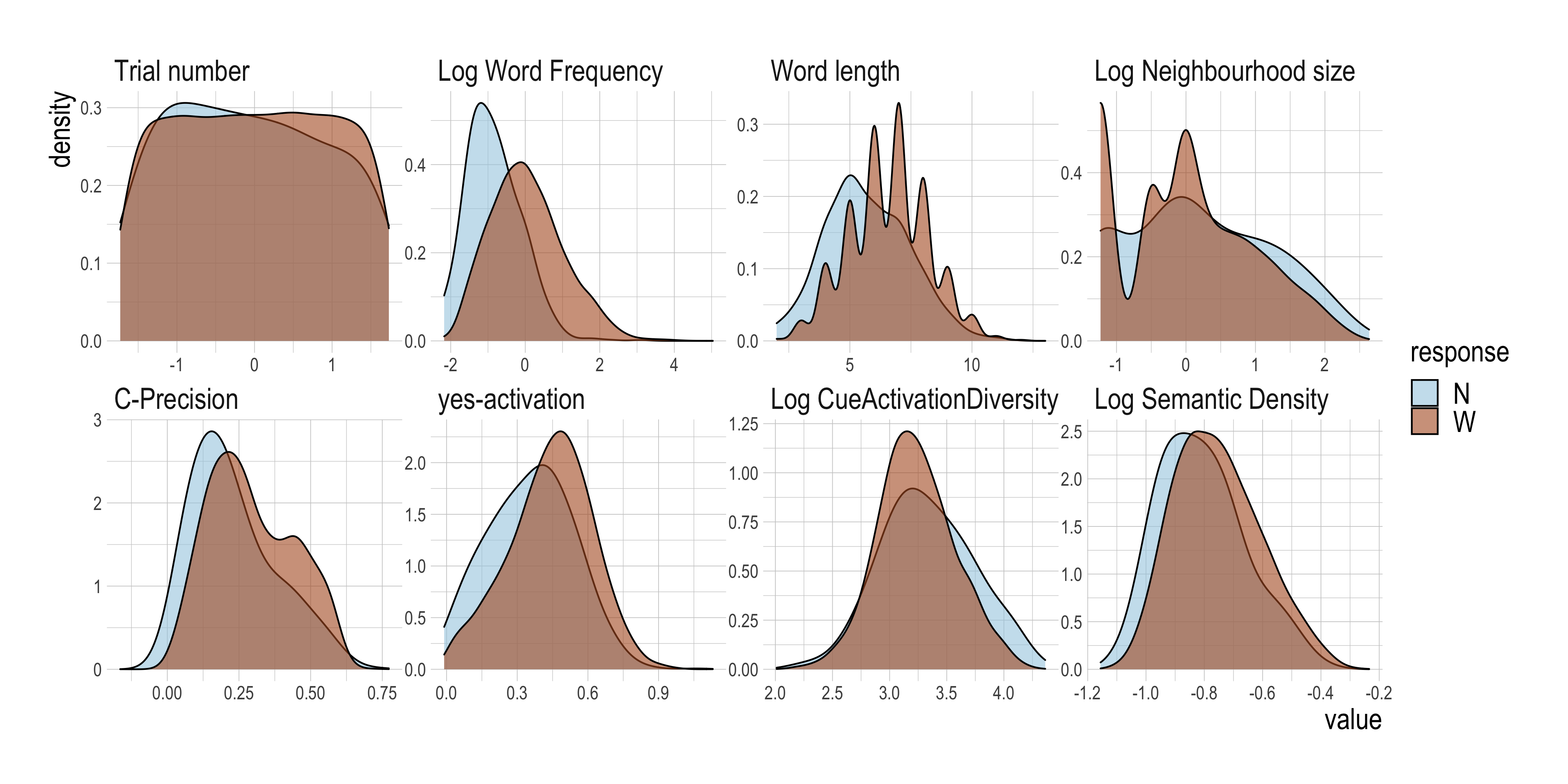
(a) Words

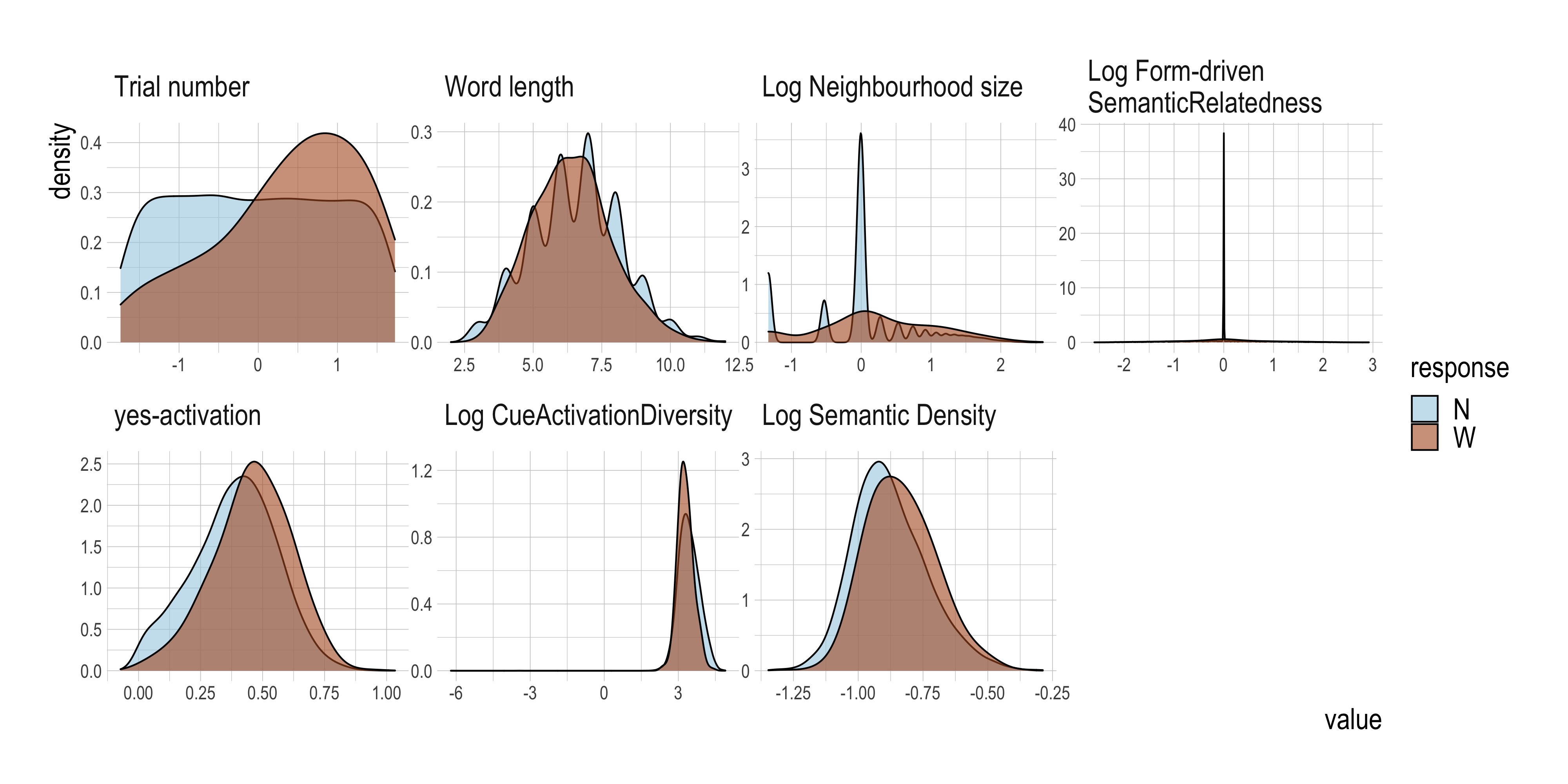
(b) Nonwords

Figure 3: Distribution of measures for words and nonwords for subject 1.

As mentioned above, given a large number of predictor variables, many of which are to some extent correlated (the maximum correlation of a pair of DLM-based predictors was $r<.6$), in order to safeguard interpretability of the partial effects of predictors in our regression models, it is crucial to bring down the number of predictors. For the full list of model-based predictors, the reader is referred to the supplementary materials.

Predictors were included in our exploratory models if, and only if, (1) their partial effect was significant ($p<0.001$), (2) including the predictor improved the overall Akaike Information Criterion (AIC; Akaike,, 1998), and (3) inclusion of a predictor did not lead to unacceptably high concurvity. We allowed for two exceptions to these rules: C-Precision in the word models and Yes-activation in the nonword models did not reach significance for one of two training subjects, but their inclusion did substantially improve model fit. These predictors were therefore retained. Further details on the validation modeling are provided in the Supplementary Materials.

5.2.3 Regression with GAMs

We used the Generalised Additive Model (GAM; Hastie and Tibshirani,, 1987; Wood,, 2011), as implemented in the mgcv package for R, to study the functional relation between response latencies and our predictor variables. GAMs are regression models that can incorporate non-linear effects of one or more predictors on the response variable (see also Baayen et al.,, 2017).

The BLP dataset is too large to allow fitting with an insightful generalized additive mixed model. To avoid this computational bottleneck, we fitted separate GAMs to the data of the individual subjects. Furthermore, for ease of interpretation, we fitted separate models to the word data and to the nonword data.

The sequences of reaction times in the BLP form time series that are characterized by autocorrelations (e.g. Baayen et al.,, 2017, 2022). GAMs can take autocorrelations into account by building an AR(1) process into the residuals, such that the residual at $t$ is a proportion $\rho$ of the residual at $t-1$ plus Gaussian noise. We obtained $\rho$ for each model individually by first extracting the autocorrelation values of residuals at lag 1 from a GAM without autocorrelation with classical predictors for both words and nonwords respectively. We then set this value as our $\rho$ for the subject, and ran both classical and DLM-based models, this time with the autocorrelation parameter included. Note that the reaction times in our GAMs are not time series in the strictest sense, as we carried out separate analyses for words and nonwords as well as excluded extreme outliers (see above).

As the original BLP experiment was too long to perform all in one session, the participants were allowed to freely choose how many blocks they wanted to do in one day. A session expired after a break of more than 10 mins between blocks. Since we assumed that after such a break, a response would no longer be influenced by the previous one, we opted to restart the autocorrelation for each new session. We experimented with never restarting and restarting only for each new day of the experiment, but found that a session-based restart addressed the issue of inter-trial autocorrelation with greater precision for our validation data.

Model criticism revealed that the de-correlated residuals did not follow Gaussian distributions. As a consequence, our models remain approximate. To ensure that these approximate models are reasonable, we also considered Gaussian location-scale models, which model the effect of predictor variables on both mean and variance of the dependent variables, as well as Quantile GAMs, which are distribution free. The functional form of partial effects remained stable across these analyses. Full details are available in the Supplementary Materials.

We complemented the GAM analyses (Sections 6.1 and 6.2) with Linear Mixed Models (LMMs) fitted to the data of all subjects jointly, with one LMM fitted to the word data, and one to the nonword data. Since participant can be included as a random-effect factor, and by allowing interactions of participant with the other predictors, the LMM becomes an eminent tool for studying individual differences between subjects.

Although it is in principle possible to use mixed GAMs, for the large dataset of the BLP, we were confronted with two problems. First, the dataset is too big for the current implementation in mgcv to estimate a model with the full complexity that we need. Second, a Generalised Additive Mixed Model with all necessary interactions, even if it were estimable, would be extremely difficult to interpret. Therefore, to study individual variation within a regression framework, we needed to simplify. The simplifying assumption that we made is that linear trends, although approximate, can be used to capture the main differences between participants.

The LMMs, which we fitted with the julia package MixedModels.jl (Bates et al.,, 2021), are reported in Section 6.3.

6 Results and Discussion

In what follows, we first present our GAMs for both words and nonwords and show how well our predictors generalise across subjects. Based on these models we then address the main question of this study, namely whether trial-to-trial learning can be detected in the BLP data. Finally, we take a closer look at individual differences between subjects.

6.1 Modeling reaction times to words and nonwords with GAMs

6.1.1 Words

GAM with Classical Predictors

We started out by fitting a baseline model using only classical psycholinguistic measures (Log Word frequency, Word length and Log Neighbourhood size) to predict reaction times. This model cannot take trial-to-trial learning into account. Additionally, we included Trial Number and the participant’s Response (word/nonword) as predictors. In the following, we will refer to the ratio of subjects for which an effect is significant ($\alpha=0.001$) as a predictor’s “reliability”. An overview of the various predictors, the direction of their effect and reliability can be found in Table 2.

Trial number was a significant predictor for all subjects. Inspecting the individual effects, we see that along the course of the experiment (see Figure 4), reaction times generally became shorter, with a couple of exceptional subjects who remained relatively stable and others who even slowed down. There was also considerable variability within sessions (cf. Baayen et al.,, 2017; Pham and Baayen,, 2015). Response was significant for 82% of participants. Log Word frequency was also significant for all subjects. The effect was qualitatively remarkably similar across all subjects. Higher Log Word frequency generally elicited shorter reaction times. At very high frequencies this effect was attenuated (Baayen et al.,, 2006; Keuleers et al.,, 2012). Higher Word Length (significant predictor for 87% of subjects) gave rise to longer reaction times, except for five subjects for which the effect was U-shaped. The U-shaped effect reported by Baayen, (2005) and New et al., (2006) apparently did not generalize to the majority of participants in the BLP. Finally, the most contested predictor for words, Log Neighbourhood size, was significant in 55% of cases. The direction of the effect was incoherent across subjects. For 28 of the subjects, higher Log Neighbourhood size elicited longer reaction times, whereas for 14 subjects they were shorter. The effects for the remaining subjects either were not significant or had no clear direction (one subject). This variability is presumably one of the reasons why the effect of Log Neighbourhood size was found to be so inconsistent across previous studies (Andrews,, 1992; Balota et al.,, 2004; Keuleers et al.,, 2012). It should be noted that this does not invalidate the construct of neighbourhood size, but that it is important to better understand the reason for this variability.

Predictor	Increase elicits …	Reliability
Trial number	shorter RTs (but wiggly)	100%
Log Word frequency	shorter RTs, attenuated at high frequencies	100%
Word length	longer RTs	87%
Log Neighbourhood size	65% longer RTs, 33% shorter RTs, rest U-shaped	55%
Response=W	30% shorter RTs, 70% longer RTs	82%

Table 2: Predictors and their reliability for words in the classical GAMs. Effect of increase (given for significant predictors only) is intended as a summary and may differ for individual subjects (see Figure 4 for details). Reliability gives the percentage of subjects for which the predictor (regardless of direction) is significant ($p<0.001$).

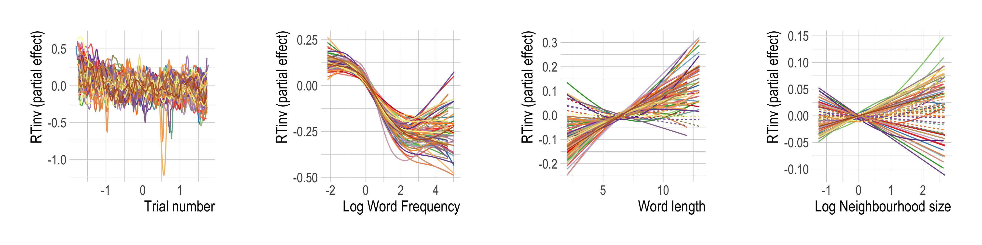
Figure 4: Partial effects of classical predictors for response latencies to words for all subjects. Solid lines are significant for $\alpha=0.001$. While the effects of Log Word frequency is very similar across all subjects, the effects of Word length and Log Neighbourhood size show substantial variability, indicative of widespread individual differences.

GAM using DLM measures

We included two sets of measures in our GAMs: a set of non-incremental measures (Trial number, Log Word frequency, Word length and Response), and four incremental measures from the DLM (Log Semantic density, Log Cue Activation Diversity, C-Precision and Yes-activation). The set of non-incremental measures does not include Orthographic Neighbourhood Size as by itself it has no clear theoretical motivation from the DLM perspective. Table 3 provides an overview of the predictors and their reliability; Figure 5 visualises the partial effects. The classical predictors in the dynamic GAMs had similar effects as in the baseline model, and are therefore not displayed (but see Supplementary Materials for further details).

Trial Number was significant across all subjects. We included this predictor because effects which arise from e.g. increased motor training, task adaption or attention fluctuations (cf. Baayen et al.,, 2022) are outside the scope of our model. We note, however, that by including Trial Number, we work against our hypothesis, as this predictor may absorb part of the effect of learning.

As expected, Log Word frequency was again significant for all subjects. Word length was a significant predictor for somewhat fewer subjects (74%), and Response for 77%.

The partial effects of the predictors that are grounded in the DLM are visualized in Figure 5. Log Semantic density (top left) was significant for 56% of all subjects: the denser the semantic space the predicted vector $\hat{\mathbf{s}}$ landed in, the faster the response. This fits well with insights gained with models such as MROM, where higher general activation implies higher lexicality — and thus faster reaction times (Grainger and Jacobs,, 1996).

Log Cue Activation Diversity (top center), a measure of the uncertainty in the $\hat{\mathbf{c}}$ vector, had high reliability for both word responses (78% of subjects) and nonword responses (90% of subjects). If the response was nonword, higher Log Cue Activation Diversity was associated with shorter reaction times (i.e. high uncertainty led to faster reaction times for nonword responses), while for word responses it elicited longer reaction times (high uncertainty led to slower reaction times).

C-Precision (bottom left), which measures how correlated the predicted vector $\hat{\mathbf{c}}$ is with the original form vector $\mathbf{c}$, was significant for about half of the subjects. For these subjects, the more precise the mapping back from the semantics to the form was, the longer reaction times were. Our interpretation of this effect is that a well-supported form vector requires suppressing the production system more, which takes resources away from making a rapid lexicality decision.

The effect of Yes-activation is displayed in the bottom center of Figure 5. Its effect was significant for 32% of subjects. For these subjects, the more sublexical evidence in favour of a word outcome (higher Yes-activation) was available, the faster participants reacted.

Predictor	Increase elicits …	Reliability
Trial number	shorter RTs (but wiggly)	100%
Log Word frequency	shorter RTs, attenuated at high frequencies	100%
Word length	longer RTs	74%
Log Semantic density	shorter RTs	56%
Log Cue Activation Diversity (word response)	longer RTs	78%
Log Cue Activation Diversity (nonword response)	shorter RTs	90%
C-Precision	longer RTs	51%
Yes-activation	shorter RTs	32%
Response=W	35% shorter RTs, 65% longer RTs	77%

Table 3: Predictors and their reliability for words in the DLM-based models. Effect of increase (given for significant predictors only) is intended as a summary and may differ for individual subjects (see Figure 5 for details). Reliability gives the percentage of subjects for which the predictor (regardless of direction) is significant ($\alpha=0.001$).

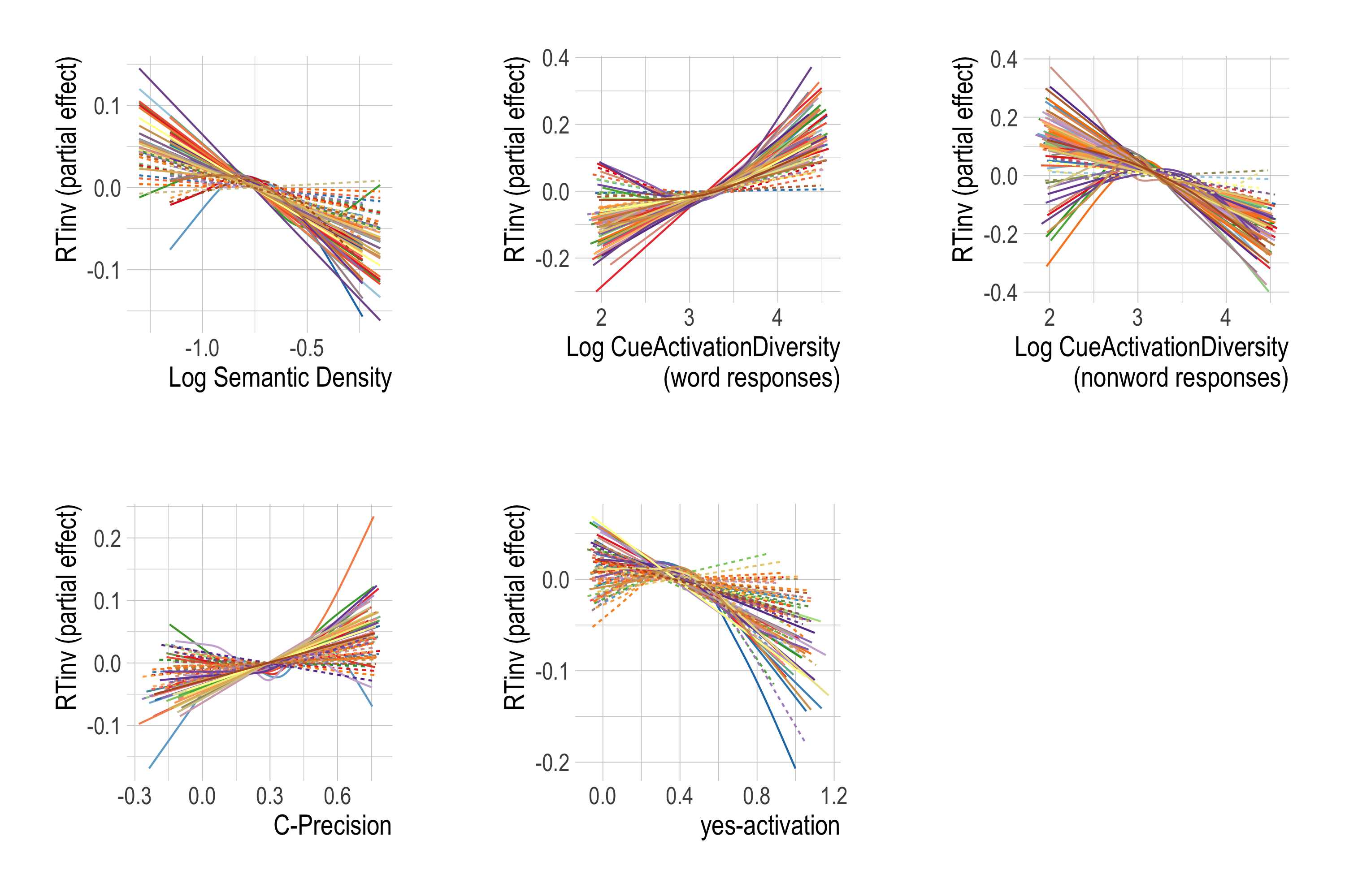
Figure 5: Partial effects of DLM predictors for all subjects (words). Solid lines have a significance level of $p<0.001$. Classical measures are omitted, as their partial effects are very similar to Figure 4. The ranges of predictors vary within plots as a consequence of the between-subject design of the BLP. Full figures can be found in the Supplementary Material.

We finally observed that 99% of the GAMs based on the DLM measures (with incremental updates) had a lower AIC value (i.e. better model fit) than the classical models (Mean AIC difference 152.6; see also Figure 8 below). In other words, the DLM-derived measures offer substantial additional precision to models based on the classical predictors only.

6.1.2 Nonwords

GAM with Classical predictors

As we had no frequencies for the nonwords in the BLP (but see Hendrix and Sun,, 2021, for the predictivity of nonword frequencies from the web for lexical decision latencies), we only included Trial number, Word length, Log Neighbourhood size and Response as classical predictors in our baseline model. Their effects are visualised in Figure 6. Overall, reaction times tended to decrease for increasing Trial Number. For both increasing Word length, and increasing Log Neighbourhood size, reaction times increased, replicating results from previous studies (Balota et al.,, 2004; Yap et al.,, 2015). All three covariates were significant for all subjects; the binary variable Response was significant for 82% of subjects (Table 4).

Predictor	Increase elicits …	Reliability
Trial number	shorter RTs (but wiggly)	100%
Word length	longer RTs	100%
Log Neighbourhood size	longer RTs	100%
Response=W	16% shorter RTs, 84% longer RTs	82%

Table 4: Predictors and their reliability for reaction times to nonwords in the classical GAMs. Effect of increase (given for significant predictors only) is intended as a summary and may differ for individual subjects (see Figure 6 for details). Reliability gives the percentage of subjects for which the predictor (regardless of direction) is significant ($\alpha=0.001$).

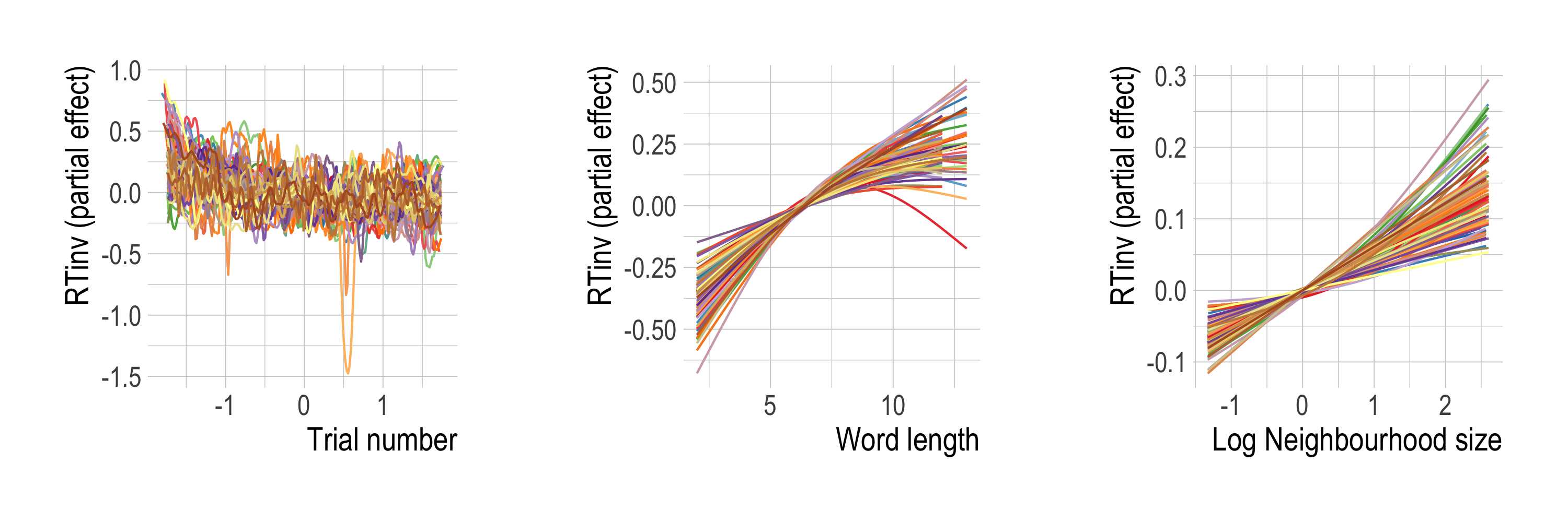
Figure 6: Partial effects of classical predictors in GAMs fitted to reaction times to nonwords, for all subjects. Solid lines are significant at $\alpha=0.001$. Effects are remarkably uniform across subjects.

GAM including DLM measures

Turning again to GAMs with DLM measures, we included Trial number and Word length as non-incremental predictors. We did not include Neighborhood Size as predictor as again, it does not have a theoretical motivation and is strongly correlated with Form-driven Semantic Relatedness (a measure that goes beyond a simple count of the number of close competitors). Unsurprisingly, both Trial number and Word length were significant for nearly all subjects and had a remarkably similar effect as in the classical models (see Supplementary Materials for visualization). Response was significant for 88% of subjects. Additionally, we found Log Form-driven Semantic Relatedness, Yes-activation, and an interaction between Log Cue Activation Diversity and Log Semantic density conditioned on response to be good predictors for nonword reaction times. These effects are summarised in Table 5 and visualised in Figure 7.

The left panel in Figure 7(a) shows the effect of Log Form-driven Semantic Relatedness, which was relatively reliable ($p<0.001$ for 71% of subjects): The more orthographic neighbours of a nonword there were, and the further apart these neighbours were in semantic space (and hence the less confusable the meanings of these neighbors are), the longer it took a subject to react to the nonword. This finding dovetails well with the effect of Log Neighbourhood size, with which it is correlated ($r=0.67$): the more orthographic neighbours a nonword has, the more it looks like a word, and the longer it takes to reject it as a word.

A higher Yes-activation, i.e. a higher support for a word outcome, predicted longer response latencies. As expected, its effect was opposite to its effect for words. While Yes-activation was only significant in 32% of subjects for words, it was significant for virtually all subjects for nonwords (99%).

One interaction emerged for the validation data, and turned out to be robust across all subjects, namely, an interaction between Log Cue Activation Diversity and Log Semantic density for nonword responses. The left three panels in the upper row of Figure 7(b) present the regression surfaces (obtained with tensor product smooths) for Subjects 53, 11 and 36. These subjects show the pattern that was typical for most subjects: higher Log Cue Activation Diversity elicited shorter reaction times, while higher Log Semantic density elicited longer reaction times specifically for lower values of Log Cue Activation Diversity. Subject 51 (upper right panel) shows a somewhat wiggly effect of Log Semantic density that is less characteristic of the full set of subjects. Plots for all subjects can be found in the Supplementary Materials.

We note here that for word responses, an interaction between Log Cue Activation Diversity and Log Semantic density was only significant for 22% of subjects, and was highly variable and inconsistent across subjects.

Predictor	Increase elicits…	Reliability
Trial number	shorter RTs (but wiggly)	100%
Word length	longer RTs	99%
Form-driven Semantic Relatedness	longer RTs	71%
Yes-activation	longer RTs	99%
N response: Sem. Density x Cue Activation Diversity	Cue Activation Diversity shorter RTs, Sem. Density longer RTs (effect stronger for lower Cue Activation Diversity)	100%
W response: Sem. Density x Cue Activation Diversity	no generalisable effect in any direction	22%
Response=W	13% shorter RTs, 87% longer RTs	88%

Table 5: Predictors and their reliability for nonwords in the DLM-based GAM models. Effect of increase (given for significant predictors only) is intended as a summary and may differ for individual subjects (see Figure 7 for details). Reliability gives the percentage of subjects for which the predictor (regardless of direction) is significant ($\alpha=0.001$).

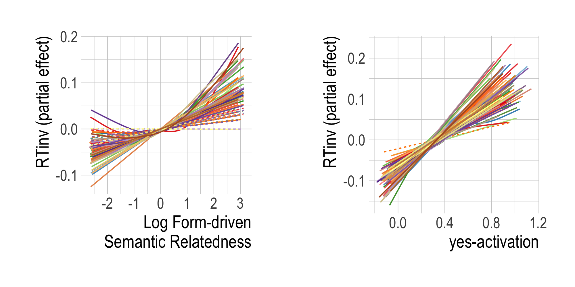
(a)

(b)

Figure 7: (a) Partial effects of the thin-plate regression smooth DLM predictors for all subjects (nonwords). Solid lines represent significance for $\alpha=0.001$. Classical measures are omitted, as they are very similar to Figure 4. (b) Sample of tensor product partial effect for nonwords with nonword responses, yellow indicates longer, and red shorter reaction times. Full figures, including those for word responses, can be found in the Supplementary Material.

Finally, the GAMs for nonwords based on DLM measures had a lower AIC (i.e. better model fit) than the classical models for all subjects (Mean AIC difference 135.3; see also Figure 8). DLM measures seem therefore well suited to also predict nonword reaction times.

6.2 Trial-to-trial learning

In order to answer the main question of this study, whether the modelling profits from incremental updates during the simulation, we ran an additional model for each subject, using the DLM-based predictors, but without ever updating these from trial to trial. This allowed us to directly compare, for any given subject, the contributions of measures obtained from a model with and a model without trial by trial learning.

The dynamic models for words had lower AIC values than the corresponding static models in 85% of cases. Differences in AIC values ranged from -40.9 (static better than dynamic) to 219.2 (dynamic better than static) (M 35.2). On average, the relative likelihood of dynamic compared to static models was $5.0\times 10^{45}$. For nonwords, dynamic models were better than static ones in 94% of cases (differences in AIC: M 55.7, range -32.7 to 208.5), with the relative likelihood of dynamic compared to the static models on average $2.5\times 10^{43}$. The differences in AIC values are presented in Figure 8. A possible explanation for some of the simulations not profiting from trial-to-trial learning is that some of these respective subjects did learn trial by trial, but the learning rate we chose was so suboptimal, that their behaviour was better approximated by the measures based on the static models, rather than the learning ones.

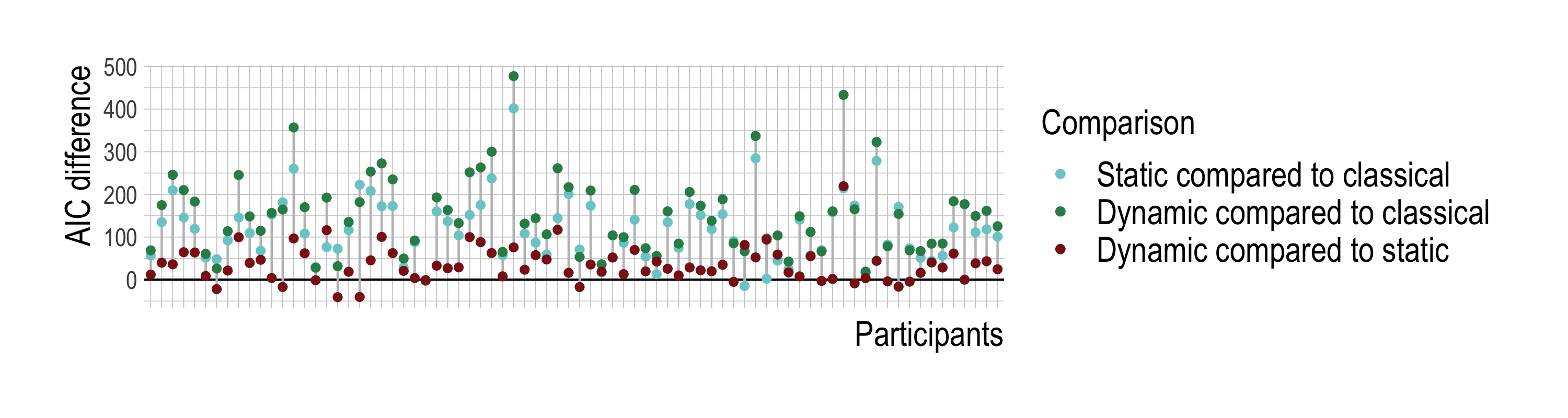
(a) Words

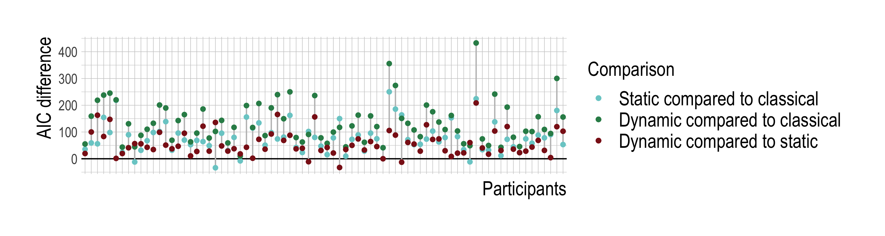
(b) Nonwords

Figure 8: AIC comparisons of classical, static (i.e. no trial-to-trial learning) and dynamic (with trial-to-trial learning) models for both words (a) and nonwords (b). If, for example, the AIC difference of “static compared to classical” (turquoise) is positive for a subject, the static GAM has a better model fit than the classical one for this particular subject. The other comparisons can be interpreted analogously. Static and dynamic models almost always have higher relative likelihood than the classical model. Dynamic models mostly show a better model fit than static models, implying that the models benefit from trial-to-trial learning.

Recall that for static models we cannot include the Yes-Activation predictor, as it is critically dependent on incremental updates. This raises the question of whether the improved model fit of dynamic simulations was due to the incremental updates of the main mapping matrices $\mathbf{F}$ and $\mathbf{G}$ during the simulation, or whether it was mainly the Yes-Activation that was responsible for improving goodness of fit. To investigate this possibility, we ran GAMs for the dynamic simulations without Yes-activation and again compared AIC values. We found that for word models, even without Yes-Activation, dynamic GAMs still provided a better model fit for 82% of the subjects, a reduction of a mere 3% (M AIC difference: 35.2). For nonwords, however, this was only the case for 60% of the subjects, a reduction by 34% (M AIC difference: 3.0). Apparently, for responses to words, trial-to-trial updating of the lexical networks contributed substantially to the goodness of fit. However, for nonwords, improvements in goodness of fit are to a much larger extent due to purely form-based sublexical learning.

6.3 Individual differences

In order to clarify the main differences between individual participants, we fitted an LMM to the reaction times for words, and a second LMM to the reaction times for nonwords. These models included by-participant random intercepts as well as by-participant random slopes for all predictors. The random effect components of the two LMMs are summarized in Table 6. The LMMs confirmed the direction of effect for all predictors, which all were well-supported ($p<0.001$), including predictors such as Yes-activation with relatively low reliability in the individual GAMs. Exceptions were the main effects as well as the interaction of Log Semantic density and Log Cue Activation Diversity for word responses in the nonword model ($p>0.68$). Possibly, this was because only 5.7% (63,274) of responses to nonwords were word responses. Additionally, the table includes information on how important the individual random slope adjustments are to the overall model fit, by providing the AIC difference that removing the respective random slope adjustment would result in.

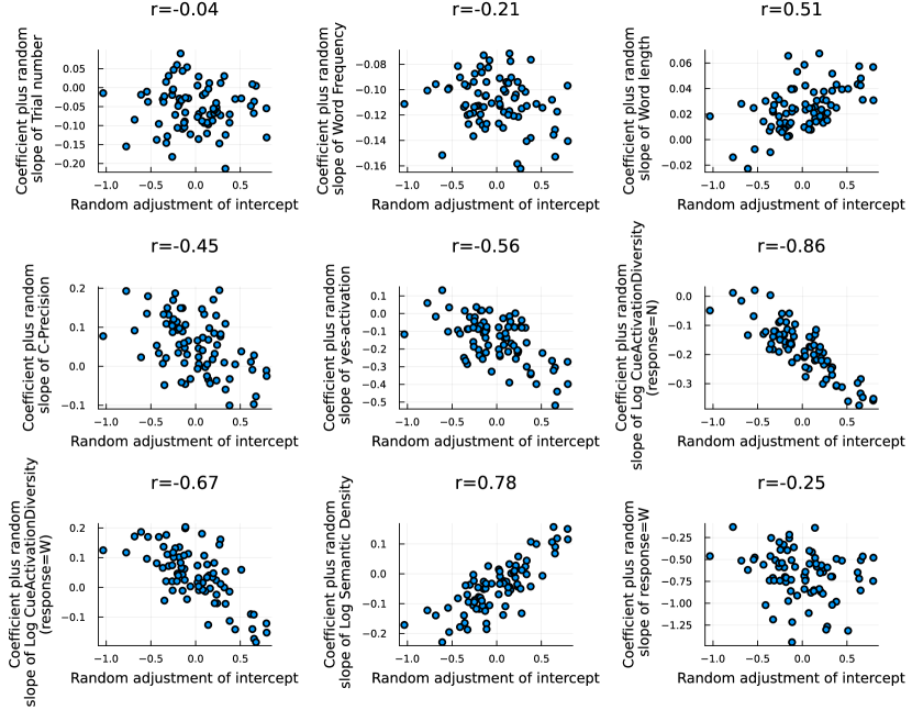
(a) Words

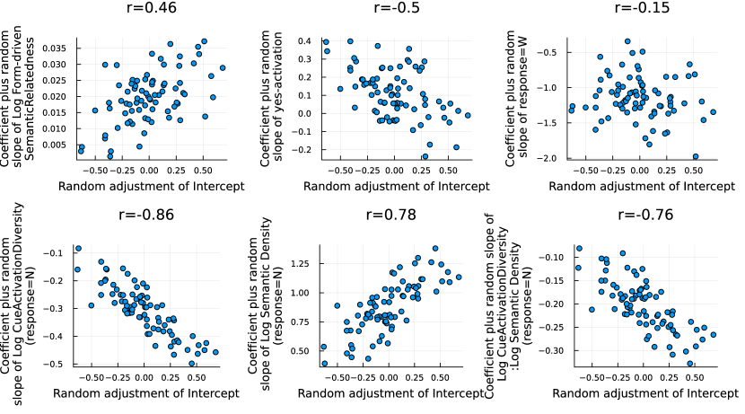
(b) Nonwords

Figure 10: Correlation between selection of participant-specific coefficients and random adjustment of intercept.

To understand subject-specific differences in the effects of our predictors, we make use of visualization by plotting by-subject random slopes against by-subject random intercepts (Figure 10). The random intercepts represent the deviation of the average response time of the individual participants from the population mean response time, with slower subjects more to the right, and faster subjects more to the left in the scatterplots in Figure 10.

First consider individual variability as revealed for the three non-incremental, classical predictors by the scatterplots in the top row of Figure 10(a) (full correlation tables can be found in the Supplementary Materials). In this figure, the y-axis concerns the participant-specific coefficients of a given predictor, i.e., the population slope $+$ the participant-specific random slope (posterior mode).

For Trial number (upper left), there is no clear correlation between random intercept and slope adjustment. For the vast majority of participants, the slope of Trial number is negative: as the experiment proceeds, participants respond more quickly. Log Word frequency (upper center) shows a weak correlation (-.21) for slopes and random intercepts, suggesting that possibly slower subjects have a stronger effect of frequency (more negative slopes; see also Kuperman and Van Dyke,, 2013). For Word length on the other hand, a clear correlation is present. For fast subjects (left side of the plot), the effect of Word length is weak or even negative, whereas for slow subjects (right side of the plot), greater word length clearly predicts longer reaction times. The correlations within the nonword model for Trial number and Word Length are very similar and not displayed in Figure 10(b), but further information is available in the Supplementary Materials. In summary, of the classical predictors, a strong correlation with response speed is present only for Word Length.

Scatterplots for the DLM-based predictors are shown in the second and third row of Figure 10(a) for words, and in Figure 10(b) for nonwords. For words (Figure 10(a)), faster subjects (with a random intercept $<0$) show large positive slopes for C-Precision (center left panel). For slower participants, the slope is close to zero, and sometimes negative. A stronger correlation is visible for Yes-Activation (center middle panel). For almost all subjects, the slope is negative, and more so for slower participants. An even stronger correlation emerges for Log Cue Activation Diversity when participants are executing nonword responses to word stimuli (center right panel). There is hardly an effect for the fastest subjects, but the slower a participant responds on average, the more negative the slope of Log Cue Activation Diversity becomes. When executing a word response, a clear negative correlation is also present (bottom left panel), but the datapoints are shifted upwards, with large positive slopes for the fastest participants, and only the very slowest subjects showing negative slopes. A strong positive correlation characterizes participants response behavior with respect to Log Semantic Density. The fastest participants show facilitation, but this effect reverses into inhibition for the slowest responders. Finally, there is no clear correlation of the slope of Response and random intercept (lower right panel).

The left-hand part of Table 7 contrasts the effects for the slower subjects as opposed to the faster subjects. The pattern that emerges is that slow subjects are primarily making use of words’ form properties. They take more time to respond to longer words, and they speed up when the orthographic features of the word provide good support for a yes response. When making a nonword response, they decide more quickly when the uncertainty of the predicted form vector is greater (Log Cue Activation Diversity). By contrast, the faster participants respond faster for words with greater semantic density, and they do not show much of an effect of word length. Faster responders appear to focus more on meaning. This explains why they respond more slowly when C-Precision is high: When the semantics precisely maps back onto form, faster responders are distracted by supporting evidence from words’ forms, having to suppress saying the word out loud. When making word responses, they also respond more slowly when Log Cue Activation Diversity is high, indicating that uncertainty about the form space is also detrimental for faster participants when presented with words.

Further insight into the individual differences between faster and slower responders is provided by the correlations in the random effects for nonwords, which are presented in Figure 10(b). A greater Log Form-driven Semantic Relatedness invariably led to longer nonword decisions (upper left panel), especially for the slower subjects. For the fastest subjects, there hardly was any effect.

Just as for responses to words, a negative correlation was present for the slopes of Yes-Activation and the random intercepts (upper center panel). But whereas for words, all but the fastest responders had negative slopes, for nonwords, negative slopes were present only for the slowest responders. In other words, slow responders made use of yes-activation to speed up their responses to words and hardly made use of yes-activation for nonwords; however, fast responders did not use yes-activation much for words, and were slowed down by this information for nonwords.

When participants made a nonword response to nonword stimuli, the slope of Log Cue Activation Diversity was always negative, and more so for slower responders (lower left panel). The same negative correlation was present for word responses to words. But whereas for words, responses were slowed down most for faster subjects, for nonwords, responses were speeded up more for slower responders. Apparently, uncertainty about the form predicted by the feedback loop differentially affected participants’ response strategies for words and nonwords.

When making nonword responses, stimuli with a greater Semantic Density (center bottom panel) elicited longer reaction times, especially for the slower responders. For nonwords, even the fast responders have positive slopes for semantic density. By contrast, for words, fast responders had negative slopes. Apparently, fast responders used dense semantic neighborhoods to respond more quickly to words, at a small cost for response speed for nonwords. Conversely, the slowest participants were hardly slowed down for words, but were especially slow to respond to nonwords in dense semantic neighborhoods.

The effects of Log Cue Activation Diversity and Log Semantic Density were modulated by a multiplicative interaction (bottom right panel). The slowing effect of Log Semantic Density is attenuated by higher values of Log Cue Activation Diversity, and most prominently so for the slower responders. Correspondingly, the negative effect of Log Cue Activation Diversity on reaction times is enhanced by higher values of Log Semantic Density, again especially so for slower responders. (For the joint effect of these predictors according to the GAM, see the example contour plots for subjects 11 and 36 in Figure 7; the estimated surfaces for these subjects are similar to sections of a hyperbolic plane, the surface modeled with a multiplicative interaction in the LMM.)

	Est.	SE	z	p	$\sigma_{\text{participant}}$	AIC diff $\sigma$
(Intercept)	-1.1370	0.0441	-25.81	$<0.0001$	0.3775
Trial number	-0.0531	0.0067	-7.98	$<0.0001$	0.0586	14,931
in_bnc=1	-0.1248	0.0060	-20.92	$<0.0001$	0.0357	37
Word length	0.0246	0.0020	12.23	$<0.0001$	0.0176	3,118
C-Precision	0.0544	0.0094	5.81	$<0.0001$	0.0764	353
Yes-activation	-0.1517	0.0151	-10.05	$<0.0001$	0.1302	1,472
Log Semantic density	-0.0450	0.0103	-4.35	$<0.0001$	0.0870	703
response=W	-0.6712	0.0330	-20.36	$<0.0001$	0.2817	936
Log Word frequency & in_bnc	-0.1100	0.0023	-47.74	$<0.0001$	0.0200	1,869
Log Cue Activation Diversity (response=N)	-0.1832	0.0108	-16.90	$<0.0001$	0.0931	2,817
Log Cue Activation Diversity (response=W)	0.0380	0.0107	3.55	0.0004	0.0928
Residual	0.3883

(a) Words

	Est.	SE	z	p	$\sigma_{\text{participant}}$	AIC diff $\sigma$
(Intercept)	-0.8557	0.0423	-20.21	$<0.0001$	0.3237
Trial number	-0.0628	0.0069	-9.08	$<0.0001$	0.0610	20,621
Word length	0.0470	0.0018	26.37	$<0.0001$	0.0154	1,686
has_neighbours_path=1	0.0718	0.0026	27.12	$<0.0001$	0.0218	406
Yes-activation	0.1135	0.0162	6.99	$<0.0001$	0.1406	1,726
response=W	-1.1454	0.0983	-11.65	$<0.0001$	0.3793	9
Log Form-driven Semantic Relatedness & has_neighbours_path	0.0198	0.0012	16.90	$<0.0001$	0.0091	140
Log Cue Activation Diversity (response=N)	-0.3071	0.0129	-23.75	$<0.0001$	0.1016	1,821
Log Cue Activation Diversity (response=W)	0.0020	0.0294	0.07	0.9450	0.1306
Log Semantic density (response=N)	0.8793	0.0366	24.05	$<0.0001$	0.2541
Log Semantic density (response=W)	0.0119	0.1090	0.11	0.9134	0.4063
Log Cue Activation Diversity & Log Semantic density (response=N)	-0.2038	0.0096	-21.30	$<0.0001$	0.0630
Log Cue Activation Diversity & Log Semantic density (response=W)	-0.0133	0.0322	-0.41	0.6795	0.1212
Residual	0.3841

(b) Nonwords

Table 6: Intercepts and random slopes estimated by the LMMs for words (a) and nonwords (b). Factors are treatment-coded. “AIC diff $\sigma$” indicates the change in AIC if the pertinent random slope is removed.

	Words		Nonwords
	strong effect	weak/reversed effect	strong effect	weak/reversed effect
Slower subjects	Word length, Yes-activation, Log Cue Activation Diversity (response=N)	Log Cue Activation Diversity (response=W), Log Semantic density, C-Precision	Word length, Log Semantic density (response=N), Log Form-driven Semantic Relatedness, Log Cue Activation Diversity (response=N), Log Cue Activation Diversity:Log Semantic density (response=N)	Yes-activation
Faster subjects	Log Cue Activation Diversity (response=W), Log Semantic density, C-Precision	Word length, Yes-activation, Log Cue Activation Diversity (response=N)	Yes-activation	Word length, Log Semantic density (response=N), Log Cue Activation Diversity (response=N), Log Form-driven Semantic Relatedness, Log Cue Activation Diversity:Log Semantic density (response=N)

Table 7: Summary table of individual differences in predictor strengths, for slower and faster subjects. Faster subjects optimize their responses by focusing on meaning for words (leading to delays from form measures), and on form for nonwords. Slower subjects optimize their responses by focusing on form across words and nonwords. In addition, for nonwords, slower subjects suffer from interference from semantics.

The right part of Table 7 summarizes the effects for nonwords, contrasting faster and slower responders. The pattern that emerges from Table 7 is the following. Slower subjects focus primarily on form properties. Slower subjects are especially slow for longer words and longer nonwords. For words, they respond extra fast for greater Yes-activation, another measure of form. For nonwords, a greater uncertainty about the form predicted by the feedback loop allows slower subjects to respond especially quickly. At the same time, measures of meaning predict especially elongated response times for slower responders (Log Form-driven Semantic Relatedness, Log Semantic density). This suggests that the slower subjects are attempting to make sense of nonwords’ semantics, but that this slows them down. Faster subjects, on the other hand, do not reveal solid effects of word length. When faster subjects are responding to words, they show more facilitation for Log Semantic Density, and more inhibition for two form measures, C-Precision and Log Cue Activation Diversity. For nonwords, faster subjects have larger positive slopes for Yes-Activation: when a stimulus’ form features provide better support for a word decision, faster subjects are slowed down more in their responses.

In other words, faster subjects optimize their responses by focusing on meaning for words (leading to delays from form measures), and on form for nonwords. Slower subjects optimize their responses by focusing on form across words and nonwords. In addition, for nonwords, slower subjects suffer from interference from semantics.

In the end, the question remains whether we can link these individual differences to hyperparameters of the DLM. Theoretically, there are three such parameters which were held constant across all participants: first, the prior knowledge of the model before entering the simulation was the same for all subjects, but it is likely that differing prior knowledge gives rise to some individual differences (e.g. Kuperman and Van Dyke,, 2013). Secondly, the two learning rates for Yes-Activation and for “lexical” learning were held constant for all participants. It is possible that for some subjects, the effects of our measures could not play out because they were based on suboptimal learning rates. While we have not explored these hyperparameters in-depth in the present study, the presented effects can inform future work investigating subject-specific hyperparameters underlying individual differences.

7 Conclusion

We set out with the hypothesis that humans’ lexical knowledge is continuously changing according to our experiences and environment. More specifically, we proposed that humans continuously learn and update their mental lexicons, from word use to word use. Since it is not clear how this effect can be measured in daily language use, we focused on detecting the effects of this continuous learning in psycholinguistic experiments. Therefore, the main question of this study was whether effects of within-experiment learning are present in the lexical decision task, and can be detected using incremental learning. We investigated this question by predicting the lexical decision latencies of individual participants in the British Lexicon Project (BLP; Keuleers et al.,, 2012), using the Discriminative Lexicon Model (DLM; Baayen et al.,, 2019) to simulate trial-to-trial learning. We then used predictors from this model to predict reaction times using Generalised Additive Models (GAMs). We found that our DLM-based measures provided a better model fit than “traditional” predictors (i.e. word frequency, length and orthographic neighbourhood density) to the reaction time data, from which we concluded that measures based on the DLM are indeed able to account for variance in lexical decision reaction times. We then hypothesised that measures based on DLM simulations with trial-to-trial learning updates would provide a better model fit than measures from non-learning DLM simulations. We found that for the majority of subjects, these learning-based predictors account for substantially more variance in reaction times than the corresponding predictors derived from a static DLM without incremental learning. We therefore conclude that trial-to-trial learning effects on reaction times are indeed present in the BLP, and that they can be detected with error-driven learning.

Our findings have several implications for theories of lexical representation and processing. First, several studies (e.g., Baayen et al.,, 2022; Balota et al.,, 2018; Lima and Huntsman,, 1997; Perea and Carreiras,, 2003) have documented inter-trial effects and discussed the consequences of these effects for the interpretation of experimental results. One particularly salient example is the study by Palmeri and Mack, (2015) on perceptual categorisation. In experiments where participants are supposed to learn categories by repeatedly categorising various stimuli, supposedly storing category representations in their long-term memory, participants can avoid learning these categories by using a “relative judgment strategy”: Participants can simply base their judgments on the difference between the current and the previous stimulus in the task. The resulting behaviour is indistinguishable from behaviour where participants store learned categories in long-term memory. Basing conclusions about long-term memory on the results of such an experiment poses the danger of building a theory about long term learning on inter-trial effects. The present study shows that there is a category learning component to lexical decision making as well. In the course of the experiment, participants learn to predict word/nonword status from words’ sublexical features, bypassing long-term lexical knowledge in lexical memory altogether, and use this information to inform their lexicality decision alongside information from long-term lexical knowledge. This is mediated by individual differences: for example, faster-responding participants emerged as primarily making nonword decisions based on this task-specific predictor, while relying primarily on long-term lexical knowledge for word decisions. The modeling framework that we are proposing makes it possible to tease apart these task effects from truly lexical effects.

Second, our results support the possibility that our lexical knowledge is not static, but changes continuously as part of the never-ending adaptation of our cognitive systems to the environment (Hoffman,, 2019). This has two implications: first, it supports learning-based theories of lexical processing (e.g. Harm and Seidenberg,, 2004; Seidenberg and McClelland,, 1989) and suggests that the proposed learning never ceases (see also Ramscar et al.,, 2014, 2017, for studies demonstrating the effects of life-long learning). Our lexical knowledge continues to grow, and changes not only across a life-time, but also locally, from word use to word use. Continuous recalibration is not restricted to language, but also takes place in, for instance, vision, as demonstrated by the anti-priming effects studied by Marsolek, (2008). Secondly, our results dovetail well with the general methodological law that a measurement instrument changes what it is designed to measure. The lexical decision task likewise does not simply probe participants’ lexical knowledge, it also changes this knowledge. Luce, (1995) argued many years ago that psychological models need to move from being static to being dynamic. We have shown that considerable headway can be made with incremental learning, as implemented in the DLM model.

Third, in addition to effects of trial-to-trial learning, in this study we also found that the DLM-derived measures contributed substantial increases in model fit. Model fits improved more for the predictors derived from the dynamic models that incorporated trial-to-trial learning, compared to the static DLM models. But even the predictors derived from the static model made it possible to substantially improve on models with the classical lexical predictors frequency, word length, and orthographic neighborhood size. This finding adds to previous studies demonstrating the ability of the DLM to provide additional prediction accuracy for behavioural data (Chuang and Baayen,, 2021; Gahl and Baayen,, 2022; Schmitz et al.,, 2021; Stein and Plag,, 2021). Of specific theoretical interest is that several of the DLM measures are grounded in a feedback loop (Chuang et al., 2020b, ) from the semantics back to form. For modeling speech production, the DLM also includes a feedback loop from form to meaning. The present simulation results therefore contribute evidence against strictly ‘feed-forward’ models of lexical processing, and evidence in favor of models in which comprehension and production are to some extent interleaved.

Fourth, the predictors grounded in discriminative learning also provide more detailed insight into individual differences. That individual differences exist between speakers is by itself unsurprising. Language users have different exposure to and experience with language (Gardner et al.,, 1987; Hernandez et al.,, 2021; Keuleers et al.,, 2015; Ramscar,, 2016). Furthermore, cognitive differences may affect lexical processing (e.g. Fischer-Baum et al.,, 2018; Kuperman and Van Dyke,, 2011; Lõo et al.,, 2019; Milin et al., 2017a, ; Perfetti et al.,, 2005). As a consequence, the regression weights of lexical-distributional predictors can vary significantly between participants (example in Baayen,, 2014). For the British Lexicon Project, we observed that faster subjects optimized their responses by focusing on meaning for words (leading to delays from well-supported forms), and on form for nonwords. Slower subjects, by contrast, optimized their responses by focusing on form across both words and nonwords. Furthermore, for nonwords, slower subjects suffered from interference from semantic neighbors. This variegated pattern of response strategies for words and nonwords by variables of form and meaning is not detectable with the classical lexical variables word frequency, word length, and neighborhood density. However, we expect the Orthography-Semantics Consistency measure of Marelli et al., (2015) to provide further evidence for a differentiated role of semantics in the BLP lexical decision latencies, similar to the measure of semantic density that we used.

Fifth, the present study supports the possibility that nonwords are not totally devoid of meaning. Earlier studies already presented experimental evidence for this possibility (Cassani et al.,, 2020; Chuang et al., 2020b, ). The present study adds to this an incremental perspective, in two ways. Firstly, especially slower responders took more time to reject nonwords when their predicted semantic vectors landed in a densely populated region of semantic space, and also when the predicted semantic vectors of their orthographic neighbors were spread out more widely in semantic space. Secondly, we modeled the semantics associated with the lexical category of ‘nonword’ as a continuously updated and ever changing location in semantic space, different across subjects, and within subjects updated from nonword trial to nonword trial in such a way that more recent nonword vectors were weighted more heavily. This implementation is in line with recency effects found in category learning (e.g. Jones et al.,, 2006). This highly dynamic and continuously evolving meaning of the nonword category was successful in driving the error for nonwords in trial-to-trial incremental learning.

Since our main research interest in this study was the detection of continuous changes of lexical knowledge, we did not implement a decision process. This approach differs from many previous computational models of lexical decision which generally tried to implement a decision directly as part of the model. For example, architectures based on the interactive activation model (Rumelhart and McClelland,, 1982) such as Grainger and Jacobs, (1996)’s Multiple Read-out Model use the activations of individual word nodes to inform the decision process. Norris, (2006)’s Bayesian reader implements a lexical decision mechanism based on the integration of a word’s prior probability with incoming evidence. Similar to the Bayesian Reader, the DIANA model (Ten Bosch et al.,, 2022), a model of auditory word recognition, implements different decision mechanisms depending on the task at hand. For lexical decision tasks, the activations between the highest supported word (modulated by prior probabilities, i.e. words’ frequencies) and pseudoword candidates are compared, until they differ by some threshold $\theta$. Instead of incorporating a decision mechanism directly into our model, we adopted a two-step approach. The first step is the lexical processing of the incoming stimulus, which includes a comprehension mapping from form to meaning as well as a production mapping from meaning to form, underlining the integrated nature of the word recognition process (Chuang et al., 2020b, ; Liberman and Mattingly,, 1985; Pulvermüller et al.,, 2006). Lexical processing is followed by the decision which is driven by general cognitive control processes. This approach was motivated in part by our research goal, showing that incremental discriminative learning can capture human trial-to-trial learning, but in part also by the work of Redgrave et al., (1999) and Gurney et al., (2001), who argue that decisions are made by distinct general cognitive control processes. Therefore, we made use of statistical models to establish the relative importance of various DLM-based lexical processing measures for lexical decision reaction times. However, improved insights into incremental lexical learning might be obtainable when the higher-order processes involved in lexicality decision making are modeled and allowed to feed back into the low-level processes of incremental lexical learning. The modeling of these processes is beyond the scope of the present study.

As is common in many computational modelling studies, we had to adopt a number of simplifications to avoid a combinatorial explosion of modelling decisions and to make our simulations feasible. For example, we chose a learning rate based on the data of one subject and used it across all subjects, even though individual differences in learning rate are to be expected (e.g. Ez-zizi et al.,, 2023). Furthermore, our model is based only on mappings between orthographic form and meaning and does not take into account any influences of mappings to phonology commonly assumed to be part of the reading process (e.g. Amenta et al.,, 2017; Newman et al.,, 2012). Future work should explore these aspects in more detail.

We conclude with a note on the Rescorla-Wagner and Widrow-Hoff learning rules. The learning rule of Rescorla and Wagner has been used successfully in many areas of language-related research (e.g. Ellis, 2006a, ; Ellis, 2006b, ; Nixon and Tomaschek,, 2021; Ramscar et al.,, 2013), including studies on trial-to-trial learning (Chuang and Baayen,, 2021; Lentz et al.,, 2021; Tomaschek et al.,, 2022). The learning rule of Widrow and Hoff has had much less impact in language and psychology, perhaps unsurprisingly, given the widespread use of discrete symbolic representations, especially for meanings and semantic features. But with the advent of distributional semantics, and the widespread availability of high-quality word embeddings, the learning rule of Widrow and Hoff now comes into its own. As demonstrated by the present study, it has exactly the right flexibility for trial-to-trial learning. A challenge for further research is the incorporation of more powerful algorithms from deep learning, while retaining this flexibility of learning.

References

- Abramson and Goldinger, (1997) Abramson, M. and Goldinger, S. D. (1997). What the reader’s eye tells the mind’s ear: Silent reading activates inner speech. Perception & Psychophysics, 59(7):1059–1068.
- Aguasvivas et al., (2018) Aguasvivas, J. A., Carreiras, M., Brysbaert, M., Mandera, P., Keuleers, E., and Duñabeitia, J. A. (2018). Spalex: A spanish lexical decision database from a massive online data collection. Frontiers in psychology, 9:2156.
- Akaike, (1998) Akaike, H. (1998). Information theory and an extension of the maximum likelihood principle. In Selected papers of Hirotugu Akaike, pages 199–213. Springer.
- Allenmark et al., (2021) Allenmark, F., Gokce, A., Geyer, T., Zinchenko, A., Müller, H. J., and Shi, Z. (2021). Inter-trial effects in priming of pop-out: Comparison of computational updating models. PLoS computational biology, 17(9):e1009332.
- Amenta et al., (2017) Amenta, S., Marelli, M., and Sulpizio, S. (2017). From sound to meaning: Phonology-to-semantics mapping in visual word recognition. Psychonomic bulletin & review, 24:887–893.
- Anderson and Lebiere, (1998) Anderson, J. and Lebiere, C. (1998). The Atomic Components of Thought (1st ed.). Psychology Press.
- Andrews, (1992) Andrews, S. (1992). Frequency and neighborhood effects on lexical access: Lexical similarity or orthographic redundancy? Journal of Experimental Psychology: Learning, Memory, and Cognition, 18(2):234.
- Arnold et al., (2017) Arnold, D., Tomaschek, F., Sering, K., Lopez, F., and Baayen, R. H. (2017). Words from spontaneous conversational speech can be recognized with human-like accuracy by an error-driven learning algorithm that discriminates between meanings straight from smart acoustic features, bypassing the phoneme as recognition unit. PloS one, 12(4):e0174623.
- Arnon and Ramscar, (2012) Arnon, I. and Ramscar, M. (2012). Granularity and the acquisition of grammatical gender: How order-of-acquisition affects what gets learned. Cognition, 122(3):292–305.
- Baayen et al., (2017) Baayen, H., Vasishth, S., Kliegl, R., and Bates, D. (2017). The cave of shadows: Addressing the human factor with generalized additive mixed models. Journal of Memory and Language, 94:206–234.
- Baayen, (2005) Baayen, R. H. (2005). Data mining at the intersection of psychology and linguistics. In Twenty-first century psycholinguistics: Four cornerstones, pages 69–84. Routledge.
- Baayen, (2014) Baayen, R. H. (2014). Multivariate statistics. Research methods in linguistics, page 337.
- Baayen et al., (2018) Baayen, R. H., Chuang, Y.-Y., and Blevins, J. P. (2018). Inflectional morphology with linear mappings. The Mental Lexicon, 13(2):230–268.
- Baayen et al., (2019) Baayen, R. H., Chuang, Y.-Y., Shafaei-Bajestan, E., and Blevins, J. (2019). The discriminative lexicon: A unified computational model for the lexicon and lexical processing in comprehension and production grounded not in (de) composition but in linear discriminative learning. Complexity, 2019.
- Baayen et al., (2022) Baayen, R. H., Fasiolo, M., Wood, S., and Chuang, Y.-Y. (2022). A note on the modeling of the effects of experimental time in psycholinguistic experiments. The Mental Lexicon, 17(2):178–212.
- Baayen et al., (2006) Baayen, R. H., Feldman, L. B., and Schreuder, R. (2006). Morphological influences on the recognition of monosyllabic monomorphemic words. Journal of Memory and Language, 55(2):290–313.
- Baayen et al., (2013) Baayen, R. H., Hendrix, P., and Ramscar, M. (2013). Sidestepping the combinatorial explosion: An explanation of n-gram frequency effects based on naive discriminative learning. Language and speech, 56(3):329–347.
- Baayen et al., (2016) Baayen, R. H., Milin, P., and Ramscar, M. (2016). Frequency in lexical processing. Aphasiology, 30(11):1174–1220.
- Baayen et al., (2011) Baayen, R. H., Milin, P., Đurđević, D. F., Hendrix, P., and Marelli, M. (2011). An amorphous model for morphological processing in visual comprehension based on naive discriminative learning. Psychological review, 118(3):438.
- Baayen et al., (1995) Baayen, R. H., Piepenbrock, R., and Gulikers, L. (1995). The CELEX lexical database [cd rom]. Philadelphia: Linguistic Data Consortium, University of Pennsylvania.
- Baayen and Smolka, (2020) Baayen, R. H. and Smolka, E. (2020). Modeling morphological priming in german with naive discriminative learning. Frontiers in Communication, 5:17.
- Balota et al., (2018) Balota, D. A., Aschenbrenner, A. J., and Yap, M. J. (2018). Dynamic adjustment of lexical processing in the lexical decision task: Cross-trial sequence effects. Quarterly Journal of Experimental Psychology, 71(1):37–45.
- Balota et al., (2004) Balota, D. A., Cortese, M. J., Sergent-Marshall, S. D., Spieler, D. H., and Yap, M. J. (2004). Visual word recognition of single-syllable words. Journal of experimental psychology: General, 133(2):283.
- Balota et al., (2007) Balota, D. A., Yap, M. J., Hutchison, K. A., Cortese, M. J., Kessler, B., Loftis, B., Neely, J. H., Nelson, D. L., Simpson, G. B., and Treiman, R. (2007). The english lexicon project. Behavior research methods, 39(3):445–459.
- Baroni et al., (2014) Baroni, M., Dinu, G., and Kruszewski, G. (2014). Don’t count, predict! a systematic comparison of context-counting vs. context-predicting semantic vectors. In Proceedings of the 52nd Annual Meeting of the Association for Computational Linguistics (Volume 1: Long Papers), pages 238–247.
- Bates et al., (2021) Bates, D., Alday, P., Kleinschmidt, D., Calderón, J. B. S., Zhan, L., Noack, A., Arslan, A., Bouchet-Valat, M., Kelman, T., Baldassari, A., Ehinger, B., Karrasch, D., Saba, E., Quinn, J., Hatherly, M., Piibeleht, M., Mogensen, P. K., Babayan, S., and Gagnon, Y. L. (2021). Juliastats/mixedmodels v4.3.0.
- Bennett et al., (2015) Bennett, D., Murawski, C., and Bode, S. (2015). Single-trial event-related potential correlates of belief updating. ENeuro, 2(5).
- Bowers et al., (2005) Bowers, J. S., Davis, C. J., and Hanley, D. A. (2005). Automatic semantic activation of embedded words: Is there a “hat” in “that”? Journal of Memory and Language, 52(1):131–143.
- Bröker and Ramscar, (2020) Bröker, F. and Ramscar, M. (2020). Representing absence of evidence: why algorithms and representations matter in models of language and cognition. Language, Cognition and Neuroscience, pages 1–24.
- Bruni et al., (2014) Bruni, E., Tran, N.-K., and Baroni, M. (2014). Multimodal distributional semantics. Journal of artificial intelligence research, 49:1–47.
- Brysbaert and New, (2009) Brysbaert, M. and New, B. (2009). Moving beyond Kučera and Francis: A critical evaluation of current word frequency norms and the introduction of a new and improved word frequency measure for American English. Behavior research methods, 41(4):977–990.
- Brysbaert et al., (2016) Brysbaert, M., Stevens, M., Mandera, P., and Keuleers, E. (2016). The impact of word prevalence on lexical decision times: Evidence from the dutch lexicon project 2. Journal of Experimental Psychology: Human Perception and Performance, 42(3):441.
- Buchanan et al., (2001) Buchanan, L., Westbury, C., and Burgess, C. (2001). Characterizing semantic space: Neighborhood effects in word recognition. Psychonomic Bulletin & Review, 8(3):531–544.
- Cassani et al., (2019) Cassani, G., Chuang, Y.-Y., and Baayen, R. H. (2019). On the semantics of non-words and their lexical category. Journal of Experimental Psychology: Learning, Memory, Cognition, 46(4):621–637.
- Cassani et al., (2020) Cassani, G., Chuang, Y.-Y., and Baayen, R. H. (2020). On the semantics of nonwords and their lexical category. Journal of Experimental Psychology: Learning, Memory, and Cognition, 46(4):621.
- Casserly and Pisoni, (2010) Casserly, E. D. and Pisoni, D. B. (2010). Speech perception and production. Wiley Interdisciplinary Reviews: Cognitive Science, 1(5):629–647.
- Chang et al., (2013) Chang, Y.-N., Ralph, M. L., Furber, S., and Welbourne, S. (2013). Modelling graded semantic effects in lexical decision. In Proceedings of the Annual Meeting of the Cognitive Science Society, volume 35.
- Chuang and Baayen, (2021) Chuang, Y.-Y. and Baayen, R. H. (2021). Discriminative learning and the lexicon: Ndl and ldl. In Oxford Research Encyclopedia of Linguistics.
- Chuang et al., (2023) Chuang, Y.-Y., Brown, D., Baayen, R. H., and Evans, R. (2023). Paradigm gaps are associated with weird “distributional semantics” properties: Russian defective nouns and their case and number paradigms. under revision for The Mental Lexicon.
- Chuang et al., (2022) Chuang, Y.-Y., Kang, M., Luo, X., and Baayen, R. H. (2022). Vector space morphology with linear discriminative learning. In Crepaldi, D., editor, Linguistic morphology in the mind and brain.
- (41) Chuang, Y.-Y., Lõo, K., Blevins, J. P., and Baayen, R. H. (2020a). Estonian case inflection made simple a case study in word and paradigm morphology with. In Körtvélyessy, L. and Štekauer, P., editors, Complex Words: Advances in Morphology, chapter 7, pages 119–14. Cambridge University Press.
- (42) Chuang, Y.-Y., Vollmer, M.-l., Shafaei-Bajestan, E., Gahl, S., Hendrix, P., and Baayen, R. H. (2020b). The processing of pseudoword form and meaning in production and comprehension: A computational modeling approach using linear discriminative learning. Behaviour Research Methods.
- Chumbley and Balota, (1984) Chumbley, J. I. and Balota, D. A. (1984). A word’s meaning affects the decision in lexical decision. Memory & Cognition, 12(6):590–606.
- Coltheart et al., (1977) Coltheart, M., Davelaar, E., Jonasson, J. T., and Besner, D. (1977). Access to the internal lexicon. In Dornick, S., editor, Attention and performance, volume VI, pages 535–556. Erlbaum, Hillsdale, New Jersey.
- Coltheart et al., (2001) Coltheart, M., Rastle, K., Perry, C., Langdon, R., and Ziegler, J. (2001). DRC: a dual route cascaded model of visual word recognition and reading aloud. Psychological review, 108(1):204.
- Dalal and Triggs, (2005) Dalal, N. and Triggs, B. (2005). Histograms of oriented gradients for human detection. In 2005 IEEE computer society conference on computer vision and pattern recognition (CVPR’05), volume 1, pages 886–893. Ieee.
- Danks, (2003) Danks, D. (2003). Equilibria of the rescorla–wagner model. Journal of Mathematical Psychology, 47(2):109–121.
- Davis, (2010) Davis, C. J. (2010). The spatial coding model of visual word identification. Psychological review, 117(3):713.
- Davis and Lupker, (2006) Davis, C. J. and Lupker, S. J. (2006). Masked inhibitory priming in english: evidence for lexical inhibition. Journal of Experimental Psychology: Human Perception and Performance, 32(3):668.
- Dell and Caramazza, (2008) Dell, G. S. and Caramazza, A. (2008). Introduction to special issue on computational modelling in cognitive neuropsychology. Cognitive Neuropsychology, 25(2):131–135.
- Diedrichsen et al., (2010) Diedrichsen, J., White, O., Newman, D., and Lally, N. (2010). Use-dependent and error-based learning of motor behaviors. Journal of Neuroscience, 30(15):5159–5166.
- Diependaele et al., (2012) Diependaele, K., Brysbaert, M., and Neri, P. (2012). How noisy is lexical decision? Frontiers in psychology, 3:348.
- Dijkstra and Van Heuven, (2002) Dijkstra, T. and Van Heuven, W. J. (2002). The architecture of the bilingual word recognition system: From identification to decision. Bilingualism: Language and cognition, 5(3):175–197.
- Dorfman and Glanzer, (1988) Dorfman, D. and Glanzer, M. (1988). List composition effects in lexical decision and recognition memory. Journal of Memory and Language, 27(6):633–648.
- Duffy and Crawford, (2008) Duffy, S. and Crawford, L. E. (2008). Primacy or recency effects in forming inductive categories. Memory & Cognition, 36(3):567–577.
- (56) Ellis, N. C. (2006a). Language acquisition as rational contingency learning. Applied linguistics, 27(1):1–24.
- (57) Ellis, N. C. (2006b). Selective attention and transfer phenomena in l2 acquisition: Contingency, cue competition, salience, interference, overshadowing, blocking, and perceptual learning. Applied linguistics, 27(2):164–194.
- Ellis and Sagarra, (2010) Ellis, N. C. and Sagarra, N. (2010). The bounds of adult language acquisition: Blocking and learned attention. Studies in Second Language Acquisition, 32(4):553–580.
- Ez-zizi et al., (2023) Ez-zizi, A., Divjak, D., and Milin, P. (2023). Error-correction mechanisms in language learning: Modeling individuals. Language Learning.
- Ferrand and Grainger, (1996) Ferrand, L. and Grainger, J. (1996). List context effects on masked phonological priming in the lexical decision task. Psychonomic Bulletin & Review, 3(4):515–519.
- Fischer-Baum et al., (2018) Fischer-Baum, S., Kook, J. H., Lee, Y., Ramos-Nuñez, A., and Vannucci, M. (2018). Individual differences in the neural and cognitive mechanisms of single word reading. Frontiers in human neuroscience, 12:271.
- Forbach et al., (1974) Forbach, G. B., Stanners, R. F., and Hochhaus, L. (1974). Repetition and practice effects in a lexical decision task. Memory & Cognition, 2(2):337–339.
- Forster and Davis, (1984) Forster, K. I. and Davis, C. (1984). Repetition priming and frequency attenuation in lexical access. Journal of experimental psychology: Learning, Memory, and Cognition, 10(4):680.
- Friedman and Wall, (2005) Friedman, L. and Wall, M. (2005). Graphical views of suppression and multicollinearity in multiple linear regression. The American Statistician, 59(2):127–136.
- Gahl and Baayen, (2022) Gahl, S. and Baayen, R. H. (2022). Time and thyme again: Connecting spoken word duration to models of the mental lexicon. https://osf.io/kxpaj/.
- Gardner et al., (1987) Gardner, M. K., Rothkopf, E. Z., Lapan, R., and Lafferty, T. (1987). The word frequency effect in lexical decision: Finding a frequency-based component. Memory and Cognition, 15:24–28.
- Gilden, (2001) Gilden, D. L. (2001). Cognitive emissions of 1/f noise. Psychological review, 108(1):33.
- Grainger and Jacobs, (1996) Grainger, J. and Jacobs, A. M. (1996). Orthographic processing in visual word recognition: a multiple read-out model. Psychological review, 103(3):518.
- Günther et al., (2019) Günther, F., Rinaldi, L., and Marelli, M. (2019). Vector-space models of semantic representation from a cognitive perspective: A discussion of common misconceptions. Perspectives on Psychological Science, 14(6):1006–1033.
- Gurney et al., (2001) Gurney, K., Prescott, T., and Redgrave, P. (2001). A computational model of action selection in the basal ganglia. Biol. Cybern., 84:401–423.
- Haber and Haber, (1982) Haber, L. R. and Haber, R. N. (1982). Does silent reading involve articulation? evidence from tongue twisters. The American journal of psychology, pages 409–419.
- Harm and Seidenberg, (2004) Harm, M. W. and Seidenberg, M. S. (2004). Computing the meanings of words in reading: cooperative division of labor between visual and phonological processes. Psychological review, 111(3):662.
- Harris, (1954) Harris, Z. S. (1954). Distributional Structure. WORD, 10(2-3).
- Hartsuiker and Kolk, (2001) Hartsuiker, R. J. and Kolk, H. H. (2001). Error monitoring in speech production: A computational test of the perceptual loop theory. Cognitive psychology, 42(2):113–157.
- Hastie and Tibshirani, (1987) Hastie, T. and Tibshirani, R. (1987). Generalized additive models: some applications. Journal of the American Statistical Association, 82(398):371–386.
- Heitmeier and Baayen, (2020) Heitmeier, M. and Baayen, R. H. (2020). Simulating phonological and semantic impairment of English tense inflection with linear discriminative learning. The Mental Lexicon, 15(3):385–421.
- Heitmeier et al., (2023) Heitmeier, M., Chuang, Y.-Y., Axen, S. D., and Baayen, R. H. (2023). Frequency effects in linear discriminative learning. arXiv preprint arXiv:2306.11044.
- Heitmeier et al., (2021) Heitmeier, M., Chuang, Y.-Y., and Baayen, R. H. (2021). Modeling morphology with linear discriminative learning: considerations and design choices. Frontiers in psychology, page 4929.
- Hendrix and Sun, (2021) Hendrix, P. and Sun, C. C. (2021). A word or two about nonwords: Frequency, semantic neighborhood density, and orthography-to-semantics consistency effects for nonwords in the lexical decision task. Journal of Experimental Psychology: Learning, Memory, and Cognition, 47(1):157.
- Hernandez et al., (2021) Hernandez, A. E., Ronderos, J., Bodet, J. P., Claussenius-Kalman, H., Nguyen, M. V., and Bunta, F. (2021). German in childhood and latin in adolescence: On the bidialectal nature of lexical access in english. Humanities and Social Sciences Communications, 8(1):1–12.
- Hickok, (2009) Hickok, G. (2009). The functional neuroanatomy of language. Physics of life reviews, 6(3):121–143.
- Hickok, (2014) Hickok, G. (2014). The architecture of speech production and the role of the phoneme in speech processing. Language, Cognition and Neuroscience, 29(1):2–20.
- Hickok and Poeppel, (2004) Hickok, G. and Poeppel, D. (2004). Dorsal and ventral streams: a framework for understanding aspects of the functional anatomy of language. Cognition, 92(1-2):67–99.
- Hoffman, (2019) Hoffman, D. (2019). The case against reality: Why evolution hid the truth from our eyes. WW Norton & Company.
- Hopman et al., (2018) Hopman, E., Thompson, B., Austerweil, J., and Lupyan, G. (2018). Predictors of l2 word learning accuracy: A big data investigation. In the 40th Annual Conference of the Cognitive Science Society (CogSci 2018), pages 513–518. Cognitive Science Society.
- Hoppe et al., (2022) Hoppe, D. B., Hendriks, P., Ramscar, M., and van Rij, J. (2022). An exploration of error-driven learning in simple two-layer networks from a discriminative learning perspective. Behavior Research Methods, pages 1–31.
- Jacobs and Grainger, (1994) Jacobs, A. M. and Grainger, J. (1994). Models of visual word recognition: sampling the state of the art. Journal of Experimental Psychology: Human perception and performance, 20(6):1311.
- Jones et al., (2013) Jones, M., Curran, T., Mozer, M. C., and Wilder, M. H. (2013). Sequential effects in response time reveal learning mechanisms and event representations. Psychological review, 120(3):628.
- Jones et al., (2006) Jones, M., Love, B. C., and Maddox, W. T. (2006). Recency effects as a window to generalization: separating decisional and perceptual sequential effects in category learning. Journal of Experimental Psychology: Learning, Memory, and Cognition, 32(2):316.
- Kell et al., (2017) Kell, C. A., Darquea, M., Behrens, M., Cordani, L., Keller, C., and Fuchs, S. (2017). Phonetic detail and lateralization of reading-related inner speech and of auditory and somatosensory feedback processing during overt reading. Human brain mapping, 38(1):493–508.
- Keuleers and Brysbaert, (2010) Keuleers, E. and Brysbaert, M. (2010). Wuggy: A multilingual pseudoword generator. Behavior research methods, 42(3):627–633.
- Keuleers et al., (2012) Keuleers, E., Lacey, P., Rastle, K., and Brysbaert, M. (2012). The British Lexicon Project: Lexical decision data for 28,730 monosyllabic and disyllabic English words. Behavior research methods, 44(1):287–304.
- Keuleers et al., (2015) Keuleers, E., Stevens, M., Mandera, P., and Brysbaert, M. (2015). Word knowledge in the crowd: Measuring vocabulary size and word prevalence in a massive online experiment. The Quarterly Journal of Experimental Psychology, (8):1665–1692.
- Kröger et al., (2016) Kröger, B. J., Crawford, E., Bekolay, T., and Eliasmith, C. (2016). Modeling interactions between speech production and perception: speech error detection at semantic and phonological levels and the inner speech loop. Frontiers in Computational Neuroscience, 10:51.
- Kuperman and Van Dyke, (2011) Kuperman, V. and Van Dyke, J. (2011). Individual differences in visual comprehension of morphological complexity. In Proceedings of the Annual Meeting of the Cognitive Science Society, volume 33.
- Kuperman and Van Dyke, (2013) Kuperman, V. and Van Dyke, J. A. (2013). Reassessing word frequency as a determinant of word recognition for skilled and unskilled readers. Journal of Experimental Psychology: Human Perception and Performance, 39(3):802.
- Lõo et al., (2019) Lõo, K., Toth, A., Karaca, F., and Järvikivi, J. (2019). Effects of affective ratings and individual differences in English morphological processing. In CogSci, pages 2179–2185.
- Laming, (1979) Laming, D. (1979). Autocorrelation of choice-reaction times. Acta psychologica, 43(5):381–412.
- Lentz et al., (2021) Lentz, T., Nixon, J. S., and van Rij, J. (2021). Temporal response modelling uncovers electrophysiological correlates of trial-by-trial error-driven learning. PsyArXiv: 10.31234/osf.io/dg5mw.
- Levelt, (1983) Levelt, W. J. (1983). Monitoring and self-repair in speech. Cognition, 14(1):41–104.
- Levenshtein et al., (1966) Levenshtein, V. I. et al. (1966). Binary codes capable of correcting deletions, insertions, and reversals. In Soviet physics doklady, volume 10, pages 707–710. Soviet Union.
- Liberman and Mattingly, (1985) Liberman, A. M. and Mattingly, I. G. (1985). The motor theory of speech perception revised. Cognition, 21(1):1–36.
- Lima and Huntsman, (1997) Lima, S. D. and Huntsman, L. A. (1997). Sequential dependencies in the lexical decision task. Psychological Research, 60(4):264–269.
- Linke et al., (2017) Linke, M., Bröker, F., Ramscar, M., and Baayen, H. (2017). Are baboons learning” orthographic” representations? probably not. PloS one, 12(8):e0183876.
- Luce, (1995) Luce, R. D. (1995). Four tensions concerning mathematical modeling in psychology. Annual Review of Psychology, 46:1.
- Luo, (2021) Luo, X. (2021). JudiLing: An implementation for Linear Discriminative Learning in JudiLing (unpublished Master’s thesis). https://github.com/MegamindHenry/JudiLing.jl/blob/master/thesis/thesis_JudiLing__An_implementation_for_Discriminative_Learning_in_Julia.pdf.
- Mandera et al., (2017) Mandera, P., Keuleers, E., and Brysbaert, M. (2017). Explaining human performance in psycholinguistic tasks with models of semantic similarity based on prediction and counting: A review and empirical validation. Journal of Memory and Language, 92:57–78.
- Marelli and Amenta, (2018) Marelli, M. and Amenta, S. (2018). A database of orthography-semantics consistency (osc) estimates for 15,017 english words. Behavior research methods, 50(4):1482–1495.
- Marelli et al., (2015) Marelli, M., Amenta, S., and Crepaldi, D. (2015). Semantic transparency in free stems: The effect of orthography-semantics consistency on word recognition. Quarterly Journal of Experimental Psychology, 68(8):1571–1583.
- Marsolek, (2008) Marsolek, C. J. (2008). What antipriming reveals about priming. Trends in Cognitive Sciences, 12(5):176–181.
- McClelland, (2009) McClelland, J. L. (2009). The place of modeling in cognitive science. Topics in Cognitive Science, 1(1):11–38.
- McClelland and Rumelhart, (1989) McClelland, J. L. and Rumelhart, D. E. (1989). Explorations in parallel distributed processing: A handbook of models, programs, and exercises. MIT press.
- McNamara, (2005) McNamara, T. P. (2005). Semantic priming: Perspectives from memory and word recognition. Psychology Press.
- Mikolov et al., (2013) Mikolov, T., Chen, K., Corrado, G., and Dean, J. (2013). Efficient estimation of word representations in vector space. arXiv preprint arXiv:1301.3781.
- (115) Milin, P., Divjak, D., and Baayen, R. H. (2017a). A learning perspective on individual differences in skilled reading: Exploring and exploiting orthographic and semantic discrimination cues. Journal of Experimental Psychology: Learning, Memory, and Cognition, 43(11):1730.
- (116) Milin, P., Feldman, L. B., Ramscar, M., Hendrix, P., and Baayen, R. H. (2017b). Discrimination in lexical decision. PloS one, 12(2):e0171935.
- (117) Milin, P., Madabushi, H. T., Croucher, M., and Divjak, D. (2020a). Keeping it simple: Implementation and performance of the proto-principle of adaptation and learning in the language sciences. arXiv preprint arXiv:2003.03813.
- (118) Milin, P., Nenadić, F., and Ramscar, M. (2020b). Approaching text genre: How contextualized experience shapes task-specific performance. Scientific Study of Literature, 10(1):3–34.
- Nassar et al., (2010) Nassar, M. R., Wilson, R. C., Heasly, B., and Gold, J. I. (2010). An approximately bayesian delta-rule model explains the dynamics of belief updating in a changing environment. Journal of Neuroscience, 30(37):12366–12378.
- New et al., (2006) New, B., Ferrand, L., Pallier, C., and Brysbaert, M. (2006). Re-examining word length effects in visual word recognition: New evidence from the english lexicon project. Psychonomic bulletin & review, 13:45–52.
- Newman et al., (2012) Newman, R. L., Jared, D., and Haigh, C. A. (2012). Does phonology play a role when skilled readers read high-frequency words? evidence from erps. Language and Cognitive Processes, 27(9):1361–1384.
- Nieder et al., (2021) Nieder, J., Chuang, Y.-Y., van de Vijver, R., and Baayen, R. (2021). Comprehension, production and processing of maltese plurals in the discriminative lexicon. PyArXiv preprint 10.31234/osf.io/rkath.
- Nikolaev et al., (2023) Nikolaev, A., Chuang, Y.-Y., and Baayen, R. H. (2023). A generating model for finnish nominal inflection using distributional semantics. The Mental Lexicon.
- Nixon and Tomaschek, (2021) Nixon, J. S. and Tomaschek, F. (2021). Prediction and error in early infant speech learning: A speech acquisition model. Cognition, 212:104697.
- Norris, (2006) Norris, D. (2006). The bayesian reader: explaining word recognition as an optimal bayesian decision process. Psychological review, 113(2):327.
- Norris, (2013) Norris, D. (2013). Models of visual word recognition. Trends in cognitive sciences, 17(10):517–524.
- Oppenheim et al., (2010) Oppenheim, G. M., Dell, G. S., and Schwartz, M. F. (2010). The dark side of incremental learning: A model of cumulative semantic interference during lexical access in speech production. Cognition, 114(2):227–252.
- O’Reilly et al., (2021) O’Reilly, R. C., Russin, J. L., Zolfaghar, M., and Rohrlich, J. (2021). Deep predictive learning in neocortex and pulvinar. Journal of Cognitive Neuroscience, 33(6):1158–1196.
- O’Reilly and Rohrlich, (2018) O’Reilly, R. and Rohrlich, J. (2018). Deep predictive learning in vision. In 2018 Conference on Cognitive Computational Neuroscience, pages 2018–1242.
- Palmeri and Mack, (2015) Palmeri, T. J. and Mack, M. L. (2015). How experimental trial context affects perceptual categorization. Frontiers in Psychology, 6:180.
- Pennington et al., (2014) Pennington, J., Socher, R., and Manning, C. D. (2014). Glove: Global vectors for word representation. In Empirical Methods in Natural Language Processing (EMNLP), pages 1532–1543.
- Perea and Carreiras, (2003) Perea, M. and Carreiras, M. (2003). Sequential effects in the lexical decision task: The role of the item frequency of the previous trial. Quarterly Journal of Experimental Psychology Series a Human Experimental Psychology, 56(3):385–402.
- Perfetti et al., (2005) Perfetti, C. A., Wlotko, E. W., and Hart, L. A. (2005). Word learning and individual differences in word learning reflected in event-related potentials. Journal of Experimental Psychology: Learning, Memory, and Cognition, 31(6):1281.
- Perrone-Bertolotti et al., (2012) Perrone-Bertolotti, M., Kujala, J., Vidal, J. R., Hamame, C. M., Ossandon, T., Bertrand, O., Minotti, L., Kahane, P., Jerbi, K., and Lachaux, J.-P. (2012). How silent is silent reading? intracerebral evidence for top-down activation of temporal voice areas during reading. Journal of Neuroscience, 32(49):17554–17562.
- Pferschy and Staněk, (2017) Pferschy, U. and Staněk, R. (2017). Generating subtour elimination constraints for the tsp from pure integer solutions. Central European journal of operations research, 25(1):231–260.
- Pham and Baayen, (2015) Pham, H. and Baayen, H. (2015). Vietnamese compounds show an anti-frequency effect in visual lexical decision. Language, Cognition and Neuroscience, 30(9):1077–1095.
- Pritchard et al., (2016) Pritchard, S. C., Coltheart, M., Marinus, E., and Castles, A. (2016). Modelling the implicit learning of phonological decoding from training on whole-word spellings and pronunciations. Scientific studies of reading, 20(1):49–63.
- Pulvermüller et al., (2006) Pulvermüller, F., Huss, M., Kherif, F., del Prado Martin, F. M., Hauk, O., and Shtyrov, Y. (2006). Motor cortex maps articulatory features of speech sounds. Proceedings of the National Academy of Sciences, 103(20):7865–7870.
- Ramscar, (2016) Ramscar, M. (2016). Learning and the replicability of priming effects. Current Opinion in Psychology, 12:80–84.
- Ramscar et al., (2013) Ramscar, M., Dye, M., and McCauley, S. M. (2013). Error and expectation in language learning: The curious absence of ”mouses” in adult speech. Language, pages 760–793.
- Ramscar et al., (2014) Ramscar, M., Hendrix, P., Shaoul, C., Milin, P., and Baayen, H. (2014). The myth of cognitive decline: Non-linear dynamics of lifelong learning. Topics in cognitive science, 6(1):5–42.
- Ramscar et al., (2017) Ramscar, M., Sun, C. C., Hendrix, P., and Baayen, H. (2017). The mismeasurement of mind: Life-span changes in paired-associate-learning scores reflect the “cost” of learning, not cognitive decline. Psychological science, 28(8):1171–1179.
- Ramscar and Yarlett, (2007) Ramscar, M. and Yarlett, D. (2007). Linguistic self-correction in the absence of feedback: A new approach to the logical problem of language acquisition. Cognitive science, 31(6):927–960.
- Ramscar et al., (2010) Ramscar, M., Yarlett, D., Dye, M., Denny, K., and Thorpe, K. (2010). The effects of feature-label-order and their implications for symbolic learning. Cognitive science, 34(6):909–957.
- Ratcliff, (1993) Ratcliff, R. (1993). Methods for dealing with reaction time outliers. Psychological bulletin, 114(3):510.
- Ratcliff et al., (2004) Ratcliff, R., Gomez, P., and McKoon, G. (2004). A diffusion model account of the lexical decision task. Psychological review, 111(1):159.
- Redgrave et al., (1999) Redgrave, P., Prescott, T., and Gurney, K. (1999). The basal ganglia: a vertebrate solution to the selection problem? Neuroscience, 89:1009–1023.
- Rescorla and Wagner, (1972) Rescorla, R. A. and Wagner, A. R. (1972). Classical conditioning II: current research and theory, chapter A theory of Pavlovian conitioning: variations in the effectiveness of reinforcement and nonreinforcement, pages 64–99. Appleton-Century-Crofts, New York.
- Rodd, (2004) Rodd, J. M. (2004). When do leotards get their spots? semantic activation of lexical neighbors in visual word recognition. Psychonomic Bulletin & Review, 11(3):434–439.
- Roediger, (1993) Roediger, H. L. (1993). Implicit memory in normal subjects. Handbook of neuropsychology, 8:63–131.
- Rubenstein et al., (1970) Rubenstein, H., Garfield, L., and Millikan, J. A. (1970). Homographic entries in the internal lexicon. Journal of verbal learning and verbal behavior, 9(5):487–494.
- Rumelhart et al., (1986) Rumelhart, D., Hinton, G., and Williams, R. (1986). Learning by error backpropagation. In Parallel Distributed Processing, volume 1. MIT press.
- Rumelhart and McClelland, (1982) Rumelhart, D. E. and McClelland, J. L. (1982). An interactive activation model of context effects in letter perception: Ii. the contextual enhancement effect and some tests and extensions of the model. Psychological review, 89(1):60.
- Scarborough et al., (1977) Scarborough, D. L., Cortese, C., and Scarborough, H. S. (1977). Frequency and repetition effects in lexical memory. Journal of Experimental Psychology: Human perception and performance, 3(1):1.
- Schmidt-Barbo et al., (2021) Schmidt-Barbo, P., Shafaei-Bajestan, E., and Sering, K. (2021). Predictive articulatory speech synthesis with semantic discrimination. In Studientexte zur Sprachkommunikation: Elektronische Sprachsignalverarbeitung 2021, pages 177–184. TUDpress, Dresden.
- Schmitz et al., (2021) Schmitz, D., Plag, I., Baer-Henney, D., and Stein, S. D. (2021). Durational differences of word-final/s/emerge from the lexicon: Modelling morpho-phonetic effects in pseudowords with linear discriminative learning. Frontiers in Psychology, 12:2983.
- Schultz, (1998) Schultz, W. (1998). Predictive reward signal of dopamine neurons. Journal of Neurophysiology, 80:1–27.
- Seidenberg and McClelland, (1989) Seidenberg, M. and McClelland, J. (1989). A distributed, developmental model of word recognition and naming. Psychological review, 96(4):523.
- Shafaei-Bajestan et al., (2021) Shafaei-Bajestan, E., Moradipour-Tari, M., Uhrig, P., and Baayen, R. H. (2021). Ldl-auris: a computational model, grounded in error-driven learning, for the comprehension of single spoken words. Language, Cognition and Neuroscience, pages 1–28.
- Shafaei-Bajestan et al., (2023) Shafaei-Bajestan, E., Uhrig, P., and Baayen, R. H. (2023). Making sense of spoken plurals. Under revision for the Mental Lexicon.
- Shahmohammadi et al., (2021) Shahmohammadi, H., Lensch, H. P., and Baayen, H. (2021). Learning zero-shot multifaceted visually grounded word embeddings via multi-task training. In Proceedings of the 25th Conference on Computational Natural Language Learning, pages 158–170.
- Shmueli, (2010) Shmueli, G. (2010). To explain or to predict? Statistical Science, pages 289–310.
- Skipper et al., (2017) Skipper, J. I., Devlin, J. T., and Lametti, D. R. (2017). The hearing ear is always found close to the speaking tongue: Review of the role of the motor system in speech perception. Brain and language, 164:77–105.
- Stein and Plag, (2021) Stein, S. D. and Plag, I. (2021). Morpho-phonetic effects in speech production: Modeling the acoustic duration of english derived words with linear discriminative learning. Frontiers in Psychology, 12.
- Taitz et al., (2020) Taitz, A., Assaneo, M. F., Shalom, D. E., and Trevisan, M. A. (2020). Motor representations underlie the reading of unfamiliar letter combinations. Scientific Reports, 10(1):3828.
- Ten Bosch et al., (2022) Ten Bosch, L., Boves, L., and Ernestus, M. (2022). Diana, a process-oriented model of human auditory word recognition. Brain Sciences, 12(5):681.
- Thul et al., (2021) Thul, R., Conklin, K., and Barr, D. J. (2021). Using gamms to model trial-by-trial fluctuations in experimental data: More risks but hardly any benefit. Journal of Memory and Language, 120:104247.
- Tomaschek et al., (2018) Tomaschek, F., Hendrix, P., and Baayen, R. H. (2018). Strategies for addressing collinearity in multivariate linguistic data. Journal of Phonetics, 71:249–267.
- Tomaschek et al., (2022) Tomaschek, F., Ramscar, M., and Nixon, J. (2022). The keys to the future? An examination of associative versus discriminative accounts of Serial Pattern Learning. Submitted to Cognitive Science.
- Trimmer et al., (2012) Trimmer, P. C., McNamara, J. M., Houston, A. I., and Marshall, J. A. R. (2012). Does natural selection favour the Rescorla-Wagner rule? Journal of Theoretical Biology, 302:39–52.
- Van Rijn and Anderson, (2003) Van Rijn, H. and Anderson, J. R. (2003). Modeling lexical decision as ordinary retrieval. Department of Psychology.
- Wagenmakers et al., (2008) Wagenmakers, E.-J., Ratcliff, R., Gomez, P., and McKoon, G. (2008). A diffusion model account of criterion shifts in the lexical decision task. Journal of memory and language, 58(1):140–159.
- Westbury et al., (2014) Westbury, C., Keith, J., Briesemeister, B. B., Hofmann, M. J., and Jacobs, A. M. (2014). Avoid violence, rioting, and outrage; approach celebration, delight, and strength: Using large text corpora to compute valence, arousal, and the basic emotions. The Quarterly Journal of Experimental Psychology.
- Westbury and Wurm, (2022) Westbury, C. and Wurm, L. H. (2022). Is it you you’re looking for? Personal relevance as a principal component of semantics. The Mental Lexicon, 17(1):1–33.
- Widrow and Hoff, (1960) Widrow, B. and Hoff, M. (1960). Adaptive switching circuits. 1960 WESCON Convention Record Part IV.
- Wilson and Collins, (2019) Wilson, R. C. and Collins, A. G. (2019). Ten simple rules for the computational modeling of behavioral data. Elife, 8:e49547.
- Wood, (2011) Wood, S. N. (2011). Fast stable restricted maximum likelihood and marginal likelihood estimation of semiparametric generalized linear models. Journal of the Royal Statistical Society (B), 73(1):3–36.
- Yap et al., (2015) Yap, M. J., Sibley, D. E., Balota, D. A., Ratcliff, R., and Rueckl, J. (2015). Responding to nonwords in the lexical decision task: Insights from the english lexicon project. Journal of Experimental Psychology: Learning, Memory, and Cognition, 41(3):597.