Nonlocal Drag Thermoelectricity Generated by Ferroelectric Heterostructures

Abstract

The “ferron” excitations of the electric-dipolar order carry energy as well as electric dipoles. Here we predict a nonlocal ferron drag effect in a ferroelectric on top of a metallic film: An electric current in the conductor generates a heat current in the ferroelectric by long-range charge-dipole interactions. The non-local Peltier and its reciprocal Seebeck effect can be controlled by electric gates and detected thermographically. We predict large effects for van der Waals ferroelectric films on graphene.

The electron-electron interaction between closely spaced two-dimensional electron gases (2DEGs) gives rise to non-local Coulomb drag effects gramila1991mutual ; jauho1993coulomb ; narozhny2016coulomb , in which a current in an active layer induces a voltage over the passive one. The concept of Coulomb drag has been extended to other systems and interactions. A local drag effect by the electron-phonon interaction contributes to the thermopower in bulk conductors bailyn1967phonon ; cantrell1987calculation ; lyo1988low ; vavro2003thermoelectric and also a non-local drag effect can be mediated by phonons in the spacer between the 2DEGs tso1992direct ; bonsager1998frictional ; noh1999phonon . In ferromagnetic metals, magnons, the quasiparticle excitations of local magnetization, transfer their momenta to conduction electrons by the exchange interaction. This local magnon drag effect enhances the Seebeck and Peltier coefficients bailyn1962maximum ; blatt1967magnon ; PhysRevB.13.2072 ; costache2012magnon ; flebus2016landau ; watzman2016magnon . The voltage in one layer induced by a current in the other in a heavy metal/ferromagnetic insulator/heavy metal stack is a non-local drag effect caused by spin Hall effect zhang2012magnon ; wu2016observation ; li2016observation . Theory predicts that magnons in magnetic films separated by a vacuum barrier experience a non-local drag effect by the magnetodipolar interaction liu2016nonlocal . The magnetodipolar interaction can also mediate an energy transfer through an air gap Kainuma2021 , but a non-local magnon drag effect has not yet been observed.

Ferroelectrics exhibit an electrically switchable spontaneous polarization that orders below a Curie temperature. Recently, we introduced “ferrons”, the bosonic excitations of ferroelectric order that carry elementary electric dipoles in the presence of transverse Bauer2021 ; Tang2022 or longitudinal fluctuations arXiv:2203.06367 . A direct experimental observation of the predicted polarization and heat transport phenomena, e.g. by the transient Peltier effect Bauer2021 and associated stray fields Tang2022 , may not be so simple, however.

Here we pursue ideas to simplify the detection of ferronic effects via non-local thermoelectric drag effects in bilayers of a ferroelectric and a metal, which opens new strategies for heat-to-electricity conversion. We consider a film of a perpendicularly polarized ferroelectric insulator on top of an extended metallic sheet that experiences a “ferron drag” in the form of a non-local Peltier effect, i.e., a heat current in the ferroelectric generated by an electric current in the metal film (see figure 1). We assume that the electric dipoles are all located in a common plane and that the electrons in the metal move in a parallel plane. This two-dimensional (2D) assumption is valid when the two films are separated by a distance $d$ much larger than their thickness, but certainly appropriate when the conductor is, e.g., graphene and the ferroelectric a van der Waals mono- or bilayer Chang2016 ; Liu2016 ; Li2017 ; Yang2018 ; Fei2018 ; Yuan2019 ; Yasuda2021 ; Wang2022 .

The linear response relations of transport or Ohm’s Law in our bilayer (in the $x$-direction) connect four driving forces, i.e. an in-plane electric field $E_{\mathrm{M}}$ in the metal, a gradient of an out-of-plane electric field $\partial E_{\mathrm{FE}}$ in the ferroelectric, and independent temperature gradients in the two films, with the charge current $j_{c}$ in the metal, polarization current $j_{p}$ in the ferroelectric and the heat currents $j_{q}^{(\mathrm{M})}$ and $j_{q}^{(\mathrm{FE})}$:

$$\left(\begin{array}[c]{c}-j_{c}\\ j_{q}^{(\mathrm{M})}\\ -j_{p}\\ j_{q}^{(\mathrm{FE})}\end{array}\right)=\left(\begin{array}[c]{cccc}L_{11}&L_{12}&L_{13}&L_{14}\\ L_{12}&L_{22}&L_{23}&L_{24}\\ L_{13}&L_{23}&L_{33}&L_{34}\\ L_{14}&L_{24}&L_{34}&L_{44}\end{array}\right)\left(\begin{array}[c]{c}-E_{\mathrm{M}}\\ -\partial\ln T_{\mathrm{M}}\\ \partial E_{\mathrm{FE}}\\ -\partial\ln T_{\mathrm{FE}}\end{array}\right)$$ (1)

where we already inserted the Onsager-Kelvin relation $L_{ij}=L_{ji}$ between the off-diagonal transport coefficients. We focus here on the steady state with finite $E_{\mathrm{M}}$ that induces polarization and heat currents in the ferroelectric. In the following, we disregard small thermoelectric effects in the metal, thermal leakage between the films, and electric field gradients $\partial E_{\mathrm{FE}}$ at the edges of the ferroelectric. The task then reduces to the calculation of the polarization drag $\vartheta_{D}\equiv L_{13}/L_{11}$ as well as the thermoelectric effects summarized by

$$\left(\begin{array}[c]{c}-j_{c}\\ j_{q}^{(\mathrm{FE})}\end{array}\right)=\left(\begin{array}[c]{cc}L_{11}&L_{14}\\ L_{14}&L_{44}\end{array}\right)\left(\begin{array}[c]{c}-E_{\mathrm{M}}\\ -\partial\ln T_{\mathrm{FE}}\end{array}\right)$$ (2)

in which we identify the non-local Peltier coefficient $\pi_{D}=L_{14}/L_{11}$ and thermopower $s_{D}=\pi_{D}/T_{\text{FE}}$. The electrical conductivity $\sigma=L_{11}$ is also affected by the equilibrium fluctuations of the nearby ferroelectric.

The conduction electrons in the metallic layer interact with the electric polarization $\mathbf{P}\left(\mathbf{r}\right)=P\left(\mathbf{r}_{\|}\right)\delta\left(z-d\right)\mathbf{\hat{z}}$ of the ferroelectric at $z=d$ by the electrostatic energy

$$\mathcal{H}_{\mathrm{int}}=-\int\mathbf{E}_{\mathrm{el}}\left(\mathbf{r}\right)\cdot\mathbf{P}(\mathbf{r})d\mathbf{r,}$$ (3)

where

$$\mathbf{E}_{\mathrm{el}}(\mathbf{r})=-\frac{e}{4\pi\epsilon_{r}\epsilon_{0}}\int d\mathbf{r}^{\prime}\frac{n(\mathbf{r}^{\prime})}{|\mathbf{r}-\mathbf{r}^{\prime}|^{3}}(\mathbf{r}-\mathbf{r}^{\prime})$$ (4)

is the Hartree field of the electrons, $-e$ the electron charge, $n(\mathbf{r})=n(\mathbf{r}_{\|})\delta\left(z\right)$ the electron density in the metal at $z=0$ and $\epsilon_{r}$ the relative permittivity of the separating barrier. Substituting Eq. (4) leads to

$$\mathcal{H}_{\mathrm{int}}=\frac{ed}{4\pi\epsilon_{r}\epsilon_{0}}\int\int d\mathbf{r}_{\|}d\mathbf{r}_{\|}^{\prime}\frac{P(\mathbf{r}_{\|})n(\mathbf{r}_{\|}^{\prime})}{[(\mathbf{r}_{\|}-\mathbf{r}_{\|}^{\prime})^{2}+d^{2}]^{3/2}}.$$ (5)

where $P(\mathbf{r}_{\|})$ and $n(\mathbf{r}_{\|})$ represent the 2D polarization and electron density in units of C/m and m^-2, respectively.

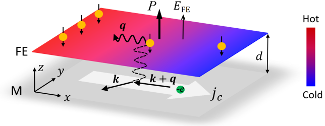
Figure 1: A schematic of the nonlocal ferron-drag Peltier effect between an extended metallic (M) and a perpendicularly polarized and electrically insulating ferroelectric (FE) film. A charge current ($j_{c}$) in the active M sheet transfers its linear momentum to the ferrons in the FE by the electrostatic interaction, leading to heat accumulations at the FE edges. The orange balls represent the ferrons, while the small black arrows are the ferron dipoles that oppose the ferroelectric order and can couple with an out-of-plane electric field ($E_{\mathrm{FE}}$).

We model the ferroelectric by the Landau-Ginzburg-Devonshire free energy Devonshire1949 ; Devonshire1951

$$F=\left(\frac{g}{2}(\boldsymbol{\nabla}P)^{2}+\frac{\alpha}{2}P^{2}+\frac{\beta}{4}P^{4}+\frac{\lambda}{6}P^{6}-E_{\mathrm{FE}}P\right)$$ (6)

where $\alpha=\alpha_{0}(T-T_{c})$, $\beta$ and $\lambda>0$ are the Landau coefficients, $T_{c}$ the Curie-Weiss temperature, $g>0$ the Ginzburg parameter accounting for the energy cost of an inhomogeneous polarization, and $E_{\text{FE}}$ is an out-of-plane electric field acting on the ferroelectric order. The phase transition for $\beta<0$ ($\beta>0$) is first (second)-order. A uniform spontaneous polarization $P_{0}$ minimizes $F$ by $\alpha P_{0}+\beta P_{0}^{3}+\lambda P_{0}^{5}=E_{\mathrm{FE}}$, which gives $P_{0}^{2}=[-\beta+(\beta^{2}-4\alpha\lambda)^{1/2}]/(2\lambda)$ when $E_{\mathrm{FE}}=0$. The non-linear static dielectric susceptibility with the field reads

$$\chi\left(E_{\mathrm{FE}}\right)=\frac{\partial P_{0}\left(E_{\mathrm{FE}}\right)}{\partial E_{\mathrm{FE}}}=\frac{1}{\alpha+3\beta P_{0}^{2}\left(E_{\mathrm{FE}}\right)+5\lambda P_{0}^{4}\left(E_{\mathrm{FE}}\right)}.$$ (7)

Small fluctuations $\delta P(\mathbf{r}_{\|},t)=P(\mathbf{r}_{\|},t)-P_{0}$ can be quantized as arXiv:2203.06367

$$\delta P(\mathbf{r}_{\|},t)=\sqrt{\frac{\hbar}{2m_{p}A}}\sum_{\mathbf{q}}\frac{\hat{a}_{\mathbf{q}}e^{i\mathbf{q}\cdot\mathbf{r}_{\|}}}{\sqrt{\omega_{q}}}+\mathrm{H.c.},$$ (8)

where $m_{p}$ is the polarization inertia that depends on the ionic masses $M_{i}$ and Born effective charges $Q_{i}$ in the unit cell of area $A_{0}$ as $m_{p}=A_{0}(\sum_{i}Q_{i}^{2}/M_{i})^{-1}$ Sivasubramanian2004 , $A$ the area of the ferroelectric sheet (assumed to be the same as the metal) and $\hat{a}_{\mathbf{q}}$ ($\hat{a}_{\mathbf{q}}^{\dagger}$) the annihilation (creation) operator of ferrons with the dispersion relation

$$\omega_{q}=\left(\frac{gq^{2}+\chi\left(E_{\mathrm{FE}}\right)^{-1}}{m_{p}}\right)^{1/2}.$$ (9)

The electric dipole carried by a single ferron is then identified as arXiv:2203.06367

$$\delta p_{q}=-\frac{\partial\hbar\omega_{q}}{\partial E_{\mathrm{FE}}}=\frac{\hbar}{2m_{p}\omega_{q}}\frac{\partial\ln\chi}{\partial P_{0}}<0$$ (10)

where the negative sign indicates its opposite direction to the ferroelectric order.

In 2D momentum space Eq. (5) now reads

$$\mathcal{H}_{\mathrm{int}}=\frac{e}{2\epsilon_{r}\epsilon_{0}A}\sum_{\mathbf{q}}e^{-dq}n(\mathbf{q})\int d\mathbf{r}_{\|}\delta{P}(\mathbf{r}_{\|})e^{i\mathbf{q}\cdot\mathbf{r}_{\|}}$$ (11)

where we dropped a constant energy shift related to $P_{0}$ and $n(\mathbf{q})=\sum_{\mathbf{k}\nu\nu^{\prime}}F_{\mathbf{k}\nu}^{\dagger}F_{(\mathbf{k}+\mathbf{q})\nu^{\prime}}\hat{c}_{\mathbf{k}\nu}^{\dagger}\hat{c}_{(\mathbf{k}+\mathbf{q})\nu^{\prime}}$ is the Fourier component of the 2D electron density in terms of the field operators $\hat{c}_{\mathbf{k}\nu}^{\dagger}$ and $\hat{c}_{\mathbf{k}\nu}$ with momentum $\mathbf{k}$, band index $\nu$ and the corresponding spinor wave functions $F_{\mathbf{k}\nu}$. $F_{\mathbf{k}^{\prime}\nu^{\prime}}^{\dagger}F_{\mathbf{k}\nu}=(e^{i(\theta_{\mathbf{k}^{\prime}}-\theta_{\mathbf{k}})}+\nu\nu^{\prime})/2$ ($=\delta_{\nu,\nu^{\prime}}$) for graphene (normal metals), where $\tan\theta_{\mathbf{k}}=k_{y}/k_{x}$ and $\nu=+1$ and $\nu=-1$ indicate the conduction and valence bands, respectively Ando2006 ; Hwang2009 . Substituting Eq. (8) yields

$$\mathcal{H}_{\mathrm{int}}=\sum_{\mathbf{k}\mathbf{q}\nu\nu^{\prime}}V_{\mathbf{k}\mathbf{q}}(\nu^{\prime},\nu)\hat{c}_{(\mathbf{k}+\mathbf{q})\nu^{\prime}}^{\dagger}\hat{c}_{\mathbf{k}\nu}\hat{a}_{\mathbf{q}}+\mathrm{H.c.},$$ (12)

where

$$V_{\mathbf{k}\mathbf{q}}(\nu^{\prime},\nu)=\frac{e}{2\epsilon_{r}\epsilon_{0}}\sqrt{\frac{\hbar}{2m_{p}A}}\frac{e^{-dq}}{\sqrt{\omega_{q}}}F_{(\mathbf{k}+\mathbf{q})\nu^{\prime}}^{\dagger}F_{\mathbf{k}\nu}$$ (13)

is the bare inelastic scattering amplitude of the electrons.

The screening by the conduction electrons and electric dipoles is a many-body problem in which $V_{\mathbf{k}\mathbf{q}}(\nu^{\prime},\nu)\rightarrow V_{\mathbf{k}\mathbf{q}}(\nu^{\prime},\nu)/\epsilon\left(q,\omega\right)$ and $\epsilon(q,\omega)$ is the dielectric function. At sufficiently high conduction electron densities, the ferron energies are small compared to the Fermi energy and we may adopt static screening $\omega\rightarrow 0$. For $q<1/(2d)\lesssim 2k_{F}$, where $k_{F}$ is the Fermi wave vector, it is sufficient to adopt the Thomas-Fermi screening approximation Stern1967 ; Ando1982 ; Ando2006 ; Hwang2007 ; Hwang2009 ; Sarma2011 , i.e.,

$$V_{\mathbf{k}\mathbf{q}}(\nu^{\prime},\nu)\rightarrow U_{\mathbf{k}\mathbf{q}}(\nu^{\prime}\nu)=\frac{V_{\mathbf{k}\mathbf{q}}(\nu^{\prime}\nu)}{1+q_{\mathrm{TF}}/q}$$ (14)

where $q_{\mathrm{TF}}=e^{2}D_{F}/(2\epsilon_{r}\epsilon_{0})$ is the 2D Thomas-Fermi wave vector in terms of the density of state $D_{F}$ at Fermi level. The screening by the ferroelectric dipoles is negligibly small compared to that of the free electrons when the ferroelectric sheet is sufficiently thin. The screening then does not depend on $d$.

We consider now the effect of a charge current $j_{c}$ driven by an electric filed ($E_{\mathrm{M}}$) along the $x$ direction in the metallic sheet that deforms the electron distribution function $f_{\mathbf{k\nu}}$ from the Fermi-Dirac form $f_{\mathbf{k}\nu}^{(0)}=[\exp\left((\varepsilon_{\mathbf{k}\nu}-\varepsilon_{F})/k_{B}T\right)+1]^{-1}$ in momentum space, where $\varepsilon_{\mathbf{k\nu}}$ is the electronic band structure, $\varepsilon_{F}$ the Fermi energy, $T$ the temperature, and $k_{B}$ Boltzmann’s constant. Within relaxation time approximation the linearized Boltzmann equation in the metal reads

$$f_{\mathbf{k\nu}}=f_{\mathbf{k}\nu}^{(0)}+e\tau_{e}v_{\mathbf{k}\nu}^{(x)}E_{M}\frac{\partial f_{\mathbf{k}\nu}^{(0)}}{\partial\varepsilon_{\mathbf{k}\nu}}$$ (15)

where $\tau_{e}$ is the relaxation time and $v_{\mathbf{k}\nu}^{(x)}=\partial\varepsilon_{\mathbf{k}\nu}/\partial\hbar k_{x}$ the group velocities in transport $(x)$ direction, with $v_{\mathbf{k}\nu}^{(x)}\rightarrow\hbar k_{x}/m_{e}$ $\left(\nu v_{F}k_{x}/|\mathbf{k}|\right)$ for a free electron gas with effective mass $m_{e}$ (or a Dirac cone of graphene with Fermi velocity $v_{F}$). The associated electric current density reads $j_{c}=\sigma E_{M}$, where

$$\sigma=\frac{e^{2}\tau_{e}\delta}{A}\sum_{\mathbf{k}}(v_{\mathbf{k}\nu}^{(x)})^{2}\left(-\frac{\partial f_{\mathbf{k}\nu}}{\partial\varepsilon_{\mathbf{k}\nu}}\right)$$ (16)

is the electrical conductivity and $\delta$ includes the spin and valley degeneracies.

In the Supplemental Material A SM we derive a ferron-electron scattering contribution that drastically reduces the $\tau_{e}$ at the Curie temperature of the ferroelectric. The observation of the predicted critical enhancement of the scattering rate would provide a proof of ferron excitations independent of the thermoelectric effects discussed in the following.

The bosonic ferron distribution function $N_{\mathbf{q}}$ in the ferroelectric is governed by another linearized Boltzmann equation arXiv:2203.06367 ; Bauer2022 . Far from the edges and in the absence of temperature or effective field gradients, the steady state distribution reads

$$N_{\mathbf{q}}=N_{q}^{(0)}+\tau_{f}\left.\frac{\partial N_{\mathbf{q}}}{\partial t}\right|_{\mathrm{int}}$$ (17)

where $N_{q}^{(0)}=\left[\exp\left(\hbar\omega_{q}/k_{B}T\right)-1\right]^{-1}$ is the equilibrium Planck distribution, $\tau_{f}$ the ferron relaxation time. The new ingredient is the collision integral $\left.\partial N_{\mathbf{q}}/\partial t\right|_{\mathrm{int}}$, which by the current in the metal and via the interlayer interaction $U_{\mathbf{q}}$ renders $N_{\mathbf{q}}\neq N_{-\mathbf{q}}.$ The electrons scatter from occupied to empty states, creating and annihilating a ferron in the process. According to Fermi’s Golden Rule

$$\left.\frac{\partial N_{\mathbf{q}}}{\partial t}\right|_{\mathrm{int}} =\frac{2\pi\delta}{\hbar}\sum_{\mathbf{k}}\left|U_{\mathbf{k}\mathbf{q}}\right|^{2}\left[(1+N_{\mathbf{q}})f_{\left(\mathbf{k}+\mathbf{q}\right)\nu}(1-f_{\mathbf{k}\nu})\right.$$

$$\left.-N_{\mathbf{q}}f_{\mathbf{k}\nu}(1-f_{\left(\mathbf{k}+\mathbf{q}\right)\nu})\right]\delta(\varepsilon_{\mathbf{k}\nu}-\varepsilon_{\left(\mathbf{k}+\mathbf{q}\right)\nu}+\hbar\omega_{q})$$ (18)

while energy and momentum are conserved. Here insignificant interband processes ($\nu\neq\nu^{\prime}$) have been discarded. To leading order, we may replace $N_{\mathbf{q}}$ on the r.h.s. of Eq. (18) with $N_{q}^{(0)}$ and substitute the distribution function of the field-biased conductor Eq. (15):

$$N_{\mathbf{q}} =N_{q}^{(0)}+\frac{2\pi\delta\tau_{f}}{\hbar}\frac{\partial N_{q}^{(0)}}{\partial\hbar\omega_{q}}\sum_{\mathbf{k}}\left|U_{\mathbf{k}\mathbf{q}}\right|^{2}(f_{\left(\mathbf{k}+\mathbf{q}\right)\nu}^{(0)}-f_{\mathbf{k}\nu}^{(0)})$$

$$\times e\tau_{e}E_{M}(v_{\mathbf{k}+\mathbf{q}}^{(x)}-v_{\mathbf{k}}^{(x)})\delta(\varepsilon_{\mathbf{k}\nu}-\varepsilon_{\left(\mathbf{k}+\mathbf{q}\right)\nu}+\hbar\omega_{q}).$$ (19)

We can now derive the non-local Peltier $\pi_{D}=-j_{q}^{(\mathrm{FE})}/j_{c}$ and polarization drag $\vartheta_{D}=j_{p}/j_{c}$ coefficients by evaluating the heat and polarization currents for the deformed ferron distribution functions by $j_{q}^{(\mathrm{FE})}=A^{-1}\sum_{\mathbf{q}}u_{\mathbf{q}}^{(x)}N_{\mathbf{q}}\hbar\omega_{q}$ and $j_{p}=A^{-1}\sum_{\mathbf{q}}u_{\mathbf{q}}^{(x)}N_{\mathbf{q}}\delta p_{q}$, respectively, where $u_{\mathbf{q}}^{(x)}=\partial\omega_{q}/\partial q_{x}$ is the ferron group velocity along $x$ direction:

$$\pi_{D}= \frac{2\pi e\tau_{f}\tau_{e}\delta}{\sigma\hbar A}\sum_{\mathbf{k}\mathbf{q}}\hbar\omega_{q}u_{\mathbf{q}}^{\left(x\right)}(v_{\mathbf{k}+\mathbf{q}}^{(x)}-v_{\mathbf{k}}^{\left(x\right)})\frac{\partial N_{q}^{(0)}}{\partial\hbar\omega_{q}}\left|U_{\mathbf{k}\mathbf{q}}\right|^{2}$$

$$\times(f_{\mathbf{k}+\mathbf{q}\nu}^{(0)}-f_{\mathbf{k}\nu}^{(0)})\delta(\varepsilon_{\mathbf{k}\nu}-\varepsilon_{\left(\mathbf{k}+\mathbf{q}\right)\nu}+\hbar\omega_{q})$$ (20)

$$\vartheta_{D}= \frac{2\pi e\tau_{f}\tau_{e}\delta}{\sigma\hbar A}\sum_{\mathbf{k}\mathbf{q}}\delta p_{q}u_{\mathbf{q}}^{\left(x\right)}(v_{\mathbf{k}+\mathbf{q}}^{(x)}-v_{\mathbf{k}}^{\left(x\right)})\frac{\partial N_{q}^{(0)}}{\partial\hbar\omega_{q}}\left|U_{\mathbf{k}\mathbf{q}}\right|^{2}$$

$$\times(f_{\mathbf{k}+\mathbf{q}\nu}^{(0)}-f_{\mathbf{k}\nu}^{(0)})\delta(\varepsilon_{\mathbf{k}\nu}-\varepsilon_{\left(\mathbf{k}+\mathbf{q}\right)\nu}+\hbar\omega_{q}).$$ (21)

We proceed by adopting the quasi-elastic approximation, i.e., $\delta(\varepsilon_{\mathbf{k}\nu}-\varepsilon_{\left(\mathbf{k}+\mathbf{q}\right)\nu}+\hbar\omega_{q})\approx\delta(\varepsilon_{\mathbf{k}\nu}-\varepsilon_{\left(\mathbf{k}+\mathbf{q}\right)\nu})$, assuming that the Fermi energy is much larger than that of the ferrons ($\lesssim 10\,$meV) arXiv:2203.06367 . This is the case in graphene with homogeneous electron densities $n_{0}>10^{12}\,$cm^-2 and Fermi energies $\varepsilon_{F}>0.11\,$eV Sarma2011 . At $k_{B}T\ll\varepsilon_{F}$, $f_{\mathbf{k}\nu}-f_{(\mathbf{k}+\mathbf{q})\nu}\simeq\hbar\omega_{q}\delta(\varepsilon_{\mathbf{k}\nu}-\varepsilon_{F})$ and we find

$$\pi_{D}\simeq \frac{e\tau_{f}g\hbar^{3}D_{F}^{2}}{32\delta m_{p}^{2}\epsilon_{0}^{2}n_{0}k_{F}k_{B}T}\int_{0}^{2k_{F}}\frac{\cos^{2}(\theta/2)q^{2}dq}{\sqrt{1-(q/2k_{F})^{2}}}$$

$$\times\frac{e^{-2dq}}{(1+q_{\mathrm{TF}}/q)^{2}}\mathrm{csch}^{2}\left(\frac{\hbar\omega_{q}}{2k_{B}T}\right).$$ (22)

In contrast to the free electron gas there is a factor $\cos^{2}(\theta/2)$ that arises from the overlap $|F_{(\mathbf{k}+\mathbf{q})\nu}^{\dagger}F_{\mathbf{k}\nu}|^{2}$, where $\theta$ is the scattering angle determined by $q=2k_{F}\sin(\theta/2)$. A similar expression can be derived for $\vartheta_{D}$ by replacing $\hbar\omega_{q}$ with $\delta p_{q}$.

The spatial separation limits the momentum transfer exponentially via the factor $\exp(-2dq)$ to $q<1/(2d)$. At large distances with $k_{F}d\gg 1$, $q_{\mathrm{TF}}d\gg 1$ and $d\gg l\equiv\sqrt{g\chi}$, only the ferrons located near the center of Brillouin zone contribute and

$$\pi_{D} \approx\frac{3\pi}{8\delta^{2}}\frac{\tau_{f}\omega_{0}}{(k_{F}d)^{3}}\left(\frac{l}{d}\right)^{2}\left(\frac{\hbar^{2}}{e^{3}m_{p}}\right)\xi_{0}\mathrm{csch}^{2}\left(\frac{\xi_{0}}{2}\right)$$

$$\simeq\frac{3\pi}{2\delta^{2}}\frac{\tau_{f}\omega_{0}}{(k_{F}d)^{3}}\left(\frac{l}{d}\right)^{2}\left(\frac{\hbar^{2}}{e^{3}m_{p}}\right)\left\{\begin{array}[c]{c}\xi_{0}e^{-\xi_{0}},\\ \xi_{0}^{-1},\end{array}\text{ for }\begin{array}[c]{c}\xi_{0}\gg 1\\ \xi_{0}\ll 1\end{array}\right.$$ (27)

$$\vartheta_{D} \approx\frac{\pi_{D}}{2}\frac{\partial\chi}{\partial P_{0}}$$ (28)

where $\xi_{0}=\hbar\omega_{0}/k_{B}T$ and $\omega_{0}=(\chi m_{p})^{-1/2}$ the ferron gap. $l\equiv\sqrt{g\chi}$ is the coherence length of the ferroelectric order, a measure of the ferroelectric domain wall width Ishibashi1989 ; Ishibashi1990 . Since magnetic domain wall widths that scale like $\sim\sqrt{J/K},$ where $J$ is the exchange interaction and $K$ is the anisotropy that governs the magnon gap, $\chi^{-1}$ plays the role of the anisotropy by stiffening the ferroelectric order.

The $T/d^{5}$ scaling relation at large distances and elevated temperatures for the drag efficiency differs from that of the Coulomb drag effect between two metallic sheets ($\sim T^{2}/d^{4}$) gramila1991mutual ; jauho1993coulomb . We can trace the difference to the faster decay of electron-dipole interactions $(\sim r^{-2})$ compared to those between charges $(\sim r^{-1})$ as a function of distance while the Planck distribution of the ferrons compared to the Fermi distribution of electrons leads to an increased phase space for scatterings at low temperatures ($k_{B}T\ll\varepsilon_{F}$).

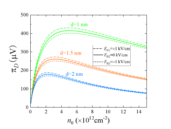
Figure 2: The nonlocal ferron-drag Peltier coefficient ($\pi_{D}$) as a function of the electron concentration ($n_{0}$) in graphene for various interlayer distance ($d$). The $\pi_{D}$ exhibit an asymmetric dependence on the relative direction of an external field ($E_{\text{FE}}$) to the ferroelectric order.

For a numerical estimate, we consider here a bilayer composed of graphene and van der Waals ferroelectric monolayer and separated by an inert h-BN layer with (out-of-plane) $\epsilon_{r}=3.76$ Laturia2018 . In graphene $\varepsilon_{\mathbf{k}\nu}=\nu\hbar v_{F}|\mathbf{k}|$ with $v_{F}=10^{8}$ cm/s, $D_{F}=2\varepsilon_{F}/(\pi\hbar^{2}v_{F}^{2})$, $\delta=4$ and $k_{F}=(4\pi n_{0}/\delta)^{1/2}$ Sarma2011 . The parameters for the ferroelectric are adopted as: $\tau_{f}=1\,$ps, $T_{c}=326\,$K, $\alpha_{0}=1.54\times 10^{3}\,$VK^-1/pC, $\beta=1.48\times 10^{5}\,$Vcm²/pC³, $\lambda=2.75\times 10^{4}\,$Vcm⁴/pC⁵ and $g=0.33\,$Vm²/C, and $m_{p}=10^{-8}\,$Vs²/C, which are close to those of the monolayer SnSe with in-plane polarization Fei2016 . Figure 2 shows the ferron-drag Peltier coefficient as a function of graphene excess electron density ($n_{0}$) for various interlayer distances $d$ at room temperature. $\pi_{D}$ has a maximum at an optimal $n_{0}$ that decreases with $d$ because a larger $n_{0}$ increases the electron-ferron scattering for small $n_{0}$ while the increased screening wins at larger densities, which is easier for larger $d$. $\pi_{D}$ depends not only on the strength, but also on the direction of an external electric field (below the coercive field), i.e., $\pi_{D}$ is reduced (enhanced) by the positive (negative) field along the ferroelectric order, because of the fact that the ferrons carry nonzero electric dipoles.

The drag effect results in heat and polarization accumulations in the ferroelectric (see figure 1). Assuming that both films are thermally isolated, a temperature gradient $T_{\mathrm{FE}}(x)=T_{0}+\partial T_{\mathrm{FE}}\left(x-L/2\right)$ emerges in a ferroelectric with length $L$, where $T_{0}$ is the ambient temperature. The open circuit condition for the heat current, i.e., $j_{q}^{(\mathrm{FE})}=-\pi_{D}j_{c}-\kappa_{\mathrm{FE}}\partial T_{\mathrm{FE}}=0$, leads to $\partial T_{\mathrm{FE}}=\left(-\pi_{D}/\kappa_{\mathrm{FE}}\right)j_{c}$, where $\kappa_{\mathrm{FE}}$ is the 2D thermal conductivity of the ferroelectric sheet (in units of W/K). The polarization accumulation $\Delta P(x)$ vanishes except for the neighborhood of the edges on the scale of the polarization relaxation length Bauer2021 .

With $d=1\,$nm, $n_{0}=10^{13}\,$cm^-2, we have $\pi_{D}=367$ $\mathrm{\mu V}$ at the room temperature. The maximum current density in graphene is limited by self-heating to $\sim 30\,$A/cm Liao2011 , but even for $j_{c}=3.4\times 10^{-2}\,$A/cm (or a bulk current density $j_{c}^{(b)}=10^{6}\,$A/cm²) this modest Peltier coefficient generates a large temperature gradient $\partial T_{\mathrm{FE}}=5$ K/$\mathrm{\mu m}$ for $\kappa_{\mathrm{FE}}=2.5\times 10^{-10}\,$W/K (or bulk $\kappa_{\mathrm{FE}}^{(b)}=0.5\,$W/Km for a monolayer thickness of $5$ Å Li2015 ) because of the simultaneous low thermal conductivity of the ferroelectric and high available current density in graphene. This should be easily observable close to the edges, even when some heat current leaks from the ferroelectric into the graphene. Inversely, a temperature gradient in the ferroelectric generates a charge current in graphene, i.e., a nonlocal ferron-drag thermopower. $s_{D}=\pi_{D}/T_{0}=1.23\,\mathrm{\mu}$V/K at $T_{0}=298\,$K. However, this number is at least an order of magnitude smaller than that of a single graphene Zuev2009 ; Wei2009 .

For sufficient thermal isolation between the ferroelectric and graphene layers the figure of merit of the ferron drag thermoelectric device can be defined and estimated as

$$\left(ZT\right)_{D}=\frac{\sigma s_{D}^{2}T_{0}}{\kappa_{\mathrm{FE}}}=2.6\times 10^{-3}$$ (29)

where $\sigma=1.38\times 10^{-3}\,$S is the electrical conductivity with the nearby ferroelectric at $n_{0}=10^{13}$ cm^-2 SM . This $\left(ZT\right)_{D}$ is comparable to that of graphene Reshak2008 but it may be engineered to become larger by, e.g., optimizing the electron density of graphene as shown in figure 2 or stacking $m$ ferroelectric monolayers with $\left(ZT\right)_{D}\propto m$ as long as all of them stay in the range of the dipolar interaction. The predicted substantial FOM in spite of the small $s_{D}$ relies on beating the Wiedemann-Franz Law that hinders conventional thermoelectric devices: The small heat conductivity in the ferroelectric does not depend on the electric conductivity in the conductor, which is large in graphene in spite of the additional ferron scattering SM .

According to Supplemental Material B SM the current drag is not specific for ferrons: the expressions are identical for in-plane longitudinal and out-of-plane polarized polar optical phonons, except for the difference in the frequency dispersions and other relevant parameters. We therefore encourage search for thermoelectric effects in any highly polarizable insulator. The attraction of using ferroelectrics is strong dependence and control of larger effects by temperature and applied electric field as well as non-volatile switching of the ferroelectric order. The critical enhancement of the electrical resistance at the Curie temperature is also unique for ferroelectrics.

Conclusion: We predict significant non-local ferron-drag thermoelectric effects in bilayers of ferroelectric insulators and conductors that are separated by a small distance $d$. A remote gate-field controlled Peltier effect can be detected by standard thermography and would prove the existence of the ferron quasiparticles in ferroelectrics. The results can be readily extended to the limit $d=0$ corresponding to van der Waals conducting ferroelectrics, known as ferroelectric metals, in which electric polarization and mobile electrons coexist Zhou2020 , and the ferroelectrics with in-plane spontaneous polarization. In the dipole approximation of the ferroelectric charge dynamics, the mobile electrons cannot screen the perpendicular ferroelectric order nor couple to the longitudinal ferrons. We may expect a strong coupling to the transverse ferrons, however, with associated interesting thermoelectric phenomena presently under investigation. Our work opens a new strategy for the design of thermoelectric devices that are not bound by the Wiedemann-Franz Law.

Acknowledgements: We acknowledge the helpful discussions with Ryo Iguchi. JSPS KAKENHI Grant No. 19H00645 supported P.T. and G.B and Grant No. 22H04965 supported G.B. and K.U. K.U. also acknowledges support by JSPS KAKENHI Grant No. 20H02609 and JST CREST “Creation of Innovative Core Technologies for Nano-enabled Thermal Management” Grant No. JPMJCR17I1.

References

- (1) T. J. Gramila, J. P. Eisenstein, A. H. MacDonald, L. N. Pfeiffer, and K. W. West, Mutual Friction between Parallel Two-Dimensional Electron Systems, Phys. Rev. Lett. 66, 1216 (1991).
- (2) A. Jauho and H. Smith, Coulomb drag between parallel two-dimensional electron systems, Phys. Rev. B 47, 4420 (1993).
- (3) B. Narozhny and A. Levchenko, Coulomb drag, Rev. Mod. Phys. 88, 025003 (2016).
- (4) M. Bailyn, Phonon-drag part of the thermoelectric power in metals, Phys. Rev. 157, 480 (1967).
- (5) D. Cantrell and P. Butcher, A calculation of the phonon-drag contribution to the thermopower of quasi-2D electrons coupled to 3D phonons, Journal of Physics C: Solid State Physics 20, 1985 (1987).
- (6) S. Lyo, Low-temperature phonon-drag thermoelectric power in heterojunctions, Phys. Rev. B 38, 6345(R) (1988).
- (7) J. Vavro, M. C. Llaguno, J. E. Fischer, S. Ramesh, R. K. Saini, L. M. Ericson, V. A. Davis, R. H. Hauge, M. Pasquali, and R. E. Smalley, Thermoelectric Power of p-Doped Single-Wall Carbon Nanotubes and the Role of Phonon Drag, Phys. Rev. Lett. 90, 065503 (2003).
- (8) H. C. Tso, P. Vasilopoulos, and F. M. Peeters, Direct Coulomb and phonon-mediated coupling between spatially separated electron gases, Phys. Rev. Lett. 68, 2516 (1992).
- (9) M. C. Bønsager, K. Flensberg, B. Y. Hu, and A. H. MacDonald, Frictional drag between quantum wells mediated by phonon exchange, Phys. Rev. B 57, 7085 (1998).
- (10) H. Noh, S. Zelakiewicz, T. J. Gramila, L. N. Pfeiffer, and K. W. West, Phonon-mediated drag in double-layer two-dimensional electron systems, Phys. Rev. B 59, 13114 (1999).
- (11) M. Bailyn, Maximum Variational Principle for Conduction Problems in a Magnetic Field, and the Theory of Magnon Drag, Phys. Rev. 126, 2040 (1962).
- (12) F. Blatt, D. Flood, V. Rowe, P. Schroeder, and J. Cox, Magnon-Drag Thermopower in Iron, Phys. Rev. Lett. 18, 395 (1967).
- (13) G. N. Grannemann and L. Berger, Magnon-drag Peltier effect in a Ni-Cu alloy, Phys. Rev. B 13, 2072 (1976).
- (14) M. V. Costache, G. Bridoux, I. Neumann and S. O. Valenzuela, Magnon-drag thermopile, Nat. Mater. 11, 199 (2012).
- (15) B. Flebus, R. A. Duine, and Y. Tserkovnyak, Landau-Lifshitz theory of the magnon-drag thermopower, Europhys. Lett. 115, 57004 (2016).
- (16) S. J. Watzman, R. A. Duine, Y. Tserkovnyak, S. R. Boona, H. Jin, A. Prakash, Y. Zheng, and J. P. Heremans, Magnon-drag thermopower and Nernst coefficient in Fe, Co, and Ni, Phys. Rev. B 94, 144407 (2016).
- (17) S. S.-L. Zhang and S. Zhang, Magnon Mediated Electric Current Drag Across a Ferromagnetic Insulator Layer, Phys. Rev. Lett. 109, 096603 (2012).
- (18) H. Wu, C. H. Wan, X. Zhang, Z. H. Yuan, Q. T. Zhang, J. Y. Qin, H. X. Wei, X. F. Han, and S. Zhang, Observation of magnon-mediated electric current drag at room temperature, Phys. Rev. B 93, 060403(R) (2016).
- (19) J. Li, Y. Xu, M. Aldosary, C. Tang, Z. Lin, S. Zhang, R. Lake, and J. Shi, Observation of magnon-mediated current drag in Pt/yttrium iron garnet/Pt(Ta) trilayers, Nat. Commun. 7, 10858 (2016).
- (20) T. Liu, G. Vignale, and M. E. Flatté, Nonlocal Drag of Magnons in a Ferromagnetic Bilayer, Phys. Rev. Lett. 116, 237202 (2016).
- (21) Y. Kainuma, R. Iguchi, D. Prananto, V. I. Vasyuchka, B. Hillebrands, T. An, and K. Uchida, Local heat emission due to unidirectional spin-wave heat conveyer effect observed by lock-in thermography, Appl. Phys. Lett. 118, 222404 (2021).
- (22) G. E. W. Bauer, R. Iguchi, and K. Uchida, Theory of transport in ferroelectric capacitors, Phys. Rev. Lett. 126, 187603 (2021).
- (23) P. Tang, R. Iguchi, K. Uchida, G. E. W. Bauer, Thermoelectric Polarization Transport in Ferroelectric Ballistic Point Contacts, Phys. Rev. Lett. 128, 047601 (2022).
- (24) P. Tang, R. Iguchi, K. Uchida, Gerrit E. W. Bauer, Excitations of the ferroelectric order, arXiv:2203.06367 (2022).
- (25) K. Chang, J. Liu, H. Lin, N. Wang, K. Zhao, A. Zhang, F. Jin, Y. Zhong, X. Hu, W. Duan, Q. Zhang, L. Fu, Qi-Kun Xue, X. Chen, and Shuai-Hua Ji, Discovery of robust in-plane ferroelectricity in atomic-thick SnTe, Science 353, 274 (2016).
- (26) F. Liu, L. You, K. L. Seyler, X. Li, P. Yu, J. Lin, X. Wang, J. Zhou, H. Wang, H. He, S. T. Pantelides, W. Zhou, P. Sharma, X. Xu, P. M. Ajayan, J. Wang, and Z. Liu, Room-temperature ferroelectricity in CuInP2S2 ultrathin flakes. Nat. Commun. 7, 12357 (2016).
- (27) L. Li and M. Wu, Binary compound bilayer and multilayer with vertical polarizations: Two-dimensional ferroelectrics, multiferroics, and nanogenerators, ACS Nano 11, 6382 (2017).
- (28) Q. Yang, M. Wu, and J. Li, Origin of two-dimensional vertical ferroelectricity in WTe2 bilayer and multilayer, J. Phys. Chem. Lett. 9, 7160 (2018).
- (29) Z. Fei, W. Zhao, T. A. Palomaki, B. Sun, M. K. Miller, Z. Zhao, J. Yan, X. Xu, and D. H. Cobden, Ferroelectric switching of a two-dimensional metal, Nature 560, 336 (2018).
- (30) S. Yuan, X. Luo, H. L. Chan, C. Xiao, Y. Dai, M. Xie, and J. Hao, Room-temperature ferroelectricity in MoTe2 down to the atomic monolayer limit, Nat. Commun. 10, 1775 (2019).
- (31) K. Yasuda, X. Wang, K. Watanabe, T. Taniguchi, P. Jarillo-Herrero, Stacking-engineered ferroelectricity in bilayer boron nitride, Science 372, 1458 (2021).
- (32) X. Wang, K. Yasuda, Y. Zhang, S. Liu, K. Watanabe, T. Taniguchi, J. Hone, L. Fu, and P. Jarillo-Herrero, Interfacial ferroelectricity in rhombohedral-stacked bilayer transition metal dichalcogenides. Nat. Nanotechnol. 17, 367 (2022).
- (33) A. F. Devonshire, Theory of barium titanate: Part I, The London, Edinburgh, and Dublin Philosophical Magazine and Journal of Science 40, 1040 (1949).
- (34) A. Devonshire, Theory of barium titanate: Part II, The London, Edinburgh, and Dublin Philosophical Magazine and Journal of Science 42, 1065 (1951).
- (35) S. Sivasubramanian, A. Widom, and Y. N. Srivastava, Physical kinetics of ferroelectric hysteresis, Ferroelectrics 300, 43 (2004).
- (36) T. Ando, Screening Effect and Impurity Scattering in Monolayer Graphene, J. Phys. Soc. Jpn. 75, 074716 (2006).
- (37) E. H. Hwang and S. D. Sarma, Screening-induced temperature-dependent transport in two-dimensional graphene, Phys. Rev. B 79, 165404 (2009).
- (38) F. Stern, Polarizability of a Two-Dimensional Electron Gas, Phys. Rev. Lett. 18, 546 (1967).
- (39) T. Ando, A. B. Fowler, and F. Stern, Electronic properties of two-dimensional systems, Rev. Mod. Phys. 54, 437 (1982).
- (40) E. H. Hwang and S. Das Sarma, Dielectric function, screening, and plasmons in two-dimensional graphene, Phys. Rev. B 75, 205418 (2007).
- (41) S. D. Sarma, S. Adam, E. H. Hwang, and E. Rossi, Electronic transport in two-dimensional graphene, Rev. Mod. Phys. 83, 407 (2011).
- (42) See the Supplemental Material for the influence of ferron-electron scatterings on the electrical conductivity in the metal and the drag effect of in-plane polarization fluctuations (polar optical phonons).
- (43) G. E. W. Bauer, P. Tang, R. Iguchi, K. Uchida, Magnonics vs. Ferronics, J. Magn. Magn. Mater. 541, 168468 (2022).
- (44) Y. Ishibashi, Phenomenological theory of domain walls, Ferroelectrics 98, 193 (1989).
- (45) Y. Ishibashi, Structure and physical properties of domain walls, Ferroelectrics 104, 299 (1990).
- (46) A. Laturia, M.L. van de Put, W.G. Vandenberghe, Dielectric properties of hexagonal boron nitride and transition metal dichalcogenides: from monolayer to bulk. npj 2D Mater Appl 2, 6 (2018).
- (47) R. Fei, W. Kang, and L. Yang, Ferroelectricity and Phase Transitions in Monolayer Group-IV Monochalcogenides, Phys. Rev. Lett. 117, 097601 (2016).
- (48) A. D. Liao, J. Z. Wu, X. Wang, K. Tahy, D. Jena, H. Dai, and E. Pop, Thermally Limited Current Carrying Ability of Graphene Nanoribbons, Phys. Rev. Lett. 106, 256801 (2011).
- (49) C. Li, J. Hong, A. May, D. Bansal, S. Chi, T. Hong, G. Ehlers, and O. Delaire, Ultralow thermal conductivity and high thermoelectric figure of merit in SnSe crystals, Nat. Phys. 11, 1063 (2015).
- (50) Y. M. Zuev, W. Chang, and P. Kim, Thermoelectric and Magnetothermoelectric Transport Measurements of Graphene, Phys. Rev. Lett. 102, 096807 (2009).
- (51) P. Wei, W. Bao, Y. Pu, C. N. Lau, and J. Shi, Anomalous Thermoelectric Transport of Dirac Particles in Graphene, Phys. Rev. Lett. 102, 166808 (2009).
- (52) A. H. Reshak, S. A. Khan and S. Auluck, Thermoelectric properties of a single graphene sheet and its derivatives, J. Mater. Chem. C 2, 2346 (2014).
- (53) W. X. Zhou and A. Ariando, Review on ferroelectric/polar metals, Jpn. J. Appl. Phys. 59, SI0802 (2020).