Quick Relaxation in Collective Motion ††thanks: This work was supported in part by NSF grant CCF-2006125.
Abstract
We establish sufficient conditions for the quick relaxation to kinetic equilibrium in the classic Vicsek-Cucker-Smale model of bird flocking. The convergence time is polynomial in the number of birds as long as the number of flocks remains bounded. This new result relies on two key ingredients: exploiting the convex geometry of embedded averaging systems; and deriving new bounds on the -energy of disconnected agreement systems. We also apply our techniques to bound the relaxation time of certain pattern-formation robotic systems investigated by Sugihara and Suzuki.
1 Introduction
In the classic Vicsek-Cucker-Smale model [7, 12], a group of birds are flying in the air while interacting via a time-varying network [2, 6, 8, 9]. The vertices of the network correspond to the birds and any two distinct birds are joined by an edge if their distance is at most some fixed . The flocking network is thus symmetric and loopless. Its connected components are the flocks. Each bird has a position and a velocity , both of them vectors in . Given the state of the system at time , we have the recurrence: for any ,
| (1) |
where is the set of vertices adjacent to at time . At each step, a bird adjusts its velocity by taking a weighted average with its neighbors. The weights indicate the amount of influence birds exercise on their neighbors. To avoid negative weights, we require that . We write . As was shown in [6], the model above might be periodic and never stabilize. To remedy this, we stipulate that, for two birds to be newly joined by an edge, their velocities must differ by at least a minimum amount: Formally, we require that, at any time , if and , for small fixed positive . By space and time scale invariance, we may assume111These bounds are arbitrary and the choice of is made only to simplify some calculations. that and for all birds . We state our main result:
Theorem 1.1
A group of birds forming a maximum of flocks relax to within of a fixed velocity vector in time , where .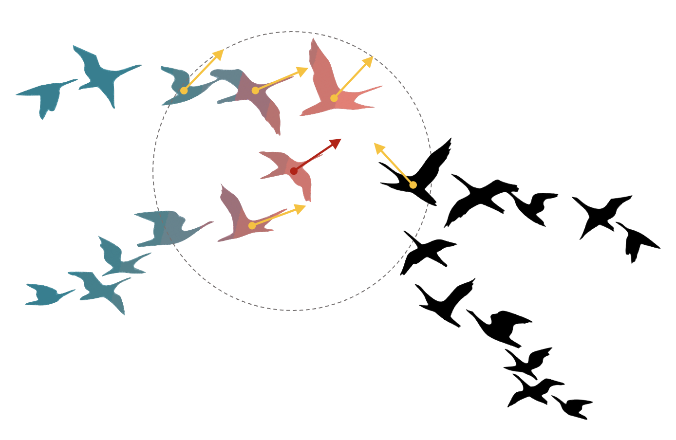
The main novelty of this result is that the convergence time is polynomial in the number of birds, as long as the number of flocks is bounded by a constant. The proof of the theorem relies on two key ingredients: new bounds on the -energy; and the specific convex geometry of flocking. In §2, we establish new (upper and lower) bounds on the -energy of reversible agreement systems. While the connected case has been well-studied [4, 5], the disconnected case was wide open. We prove a nearly tight upper bound on the -energy of such systems, which is a result of independent interest. In §3, we explore the convex geometry of flocking to bound the angle of attack between two newly joined birds as a function of time. Together with our new bounds on the -energy, this geometric insight plays a crucial part in the proof of Theorem 1.1.
In §4, we investigate a distributed motion coordination algorithm introduced by Sugihara and Suzuki [11, 3]. The idea is to use a swarm of robots to produce a preset pattern, in this case a polygon. We prove a polynomial bound on the relaxation time of this process. We enhance the model by allowing faulty communication and proving that the end result is robust under stochastic errors. We also generalize the geometry to 3D and arbitrary communication graphs.
2 Reversible Agreement Systems
Let be the stochastic matrix of a time-reversible random walk in an undirected -vertex graph . This means that , where (i) , for and constant ; and (ii) is a symmetric matrix with nonzero entries at least 1 and a positive diagonal. Given , the infinite sequence of vectors forms an orbit of a reversible averaging system (RAS). When all the matrices are the same, , the map is the dual map of the reversible Markov chain () and its convergence time is given by the mixing time of the chain. The novelty of the model lies in the presence of time-varying matrices.
2.1 The -energy
Consider an infinite sequence of graphs with the stochastic matrix of its corresponding Markov chain. Note that is proportional to the stationary distribution of the Markov chain induced by . By reversibility, we have . Write and . We call the variance of the system, where and is shorthand for .
Given , we write and we interpret as an embedding of the graph in . The union of the embedded edges of forms disjoint intervals, called blocks. Let be the lengths of these blocks and put , with . Following [5] , we define the -energy . We denote by the supremum of over all systems of unit variance whose underlying graphs have at most connected components.
2.2 An upper bound
We prove the following bound on the -energy of reversible agreement systems and then we show in §2.3 why it is close to optimal.
Theorem 2.1
, for any and constant .Proof. The convergence rate of the attracting dynamics is captured by a variant of the Dirichlet form: . We omit the index below for clarity.
Lemma 2.2
, for any .
Proof. Write and . Fix and pick any such that . By Cauchy-Schwarz and , we have
hence,
with the last equality expressing the identity for the variance: .
Write as the union of all the edges in , and let be the maximum value of such that has fewer connected components than ; if no such exists, set .
Lemma 2.3
If is connected, then .
Proof. Let denote the graph over vertices with no edges. We define as the sequence of times at which the addition of reduces the number of connected components in . At any time (), the drop in the number of components can be achieved by edges from . Let denote such a set of edges: we can always order so that every edge in the sequence contains at least one vertex not encountered yet. This shows that the sum of the squared lengths of the edges in does not exceed . We note that forms a collection of edges from (the connected graph) and spans all vertices.
Consider the intervals formed by the edges in at time , for all . The union of these intervals covers the smallest interval enclosing all the vertices at time (and hence at all times). To see why, pick any such that and denote by and the vertices on both sides of at time . Neither set is empty and, by convexity, both of them remain on their respective side of until an edge of some joins to . When that happens (which it must since is connected), the joining edge(s) reduce(s) the number of components of by at least one, so must grab at least one of them, which proves our claim. Let denote the lengths of the edges of (at the time of their insertion). By Cauchy-Schwarz, . The lemma follows from the inequalities .
Let be the maximum -energy of an RAS with at most vertices and connected components at any time, subject to the initial condition . By shifting the system if need be, we can always assume that . By (2), shrinks by at least a factor of by time . A simple scaling argument shows that the -energy expanded after is at most . While (or if is not connected), the system can be decoupled into two RAS, each one with fewer than components.222Note that each subsystem satisfies the required inequalities about the and entries; also, shifting each subsystem so that cannot increase , so its value remains at most 1. Since , the diameter at any time is at most 2; therefore . It follows that
| (3) |
hence and the proof of Theorem 2.1 is complete.
2.3 A lower bound
We begin with the case . The path graph over vertices has an edge for all . The Laplacian is , where is the adjacency matrix of and is the degree vector . We consider the RAS formed by the matrix . By well-known spectral results on graphs [10], has a full set of orthogonal eigenvectors , where for , with its associated eigenvectors , for . We require to ensure that is positive semidefinite. We initialize the system with and observe that the agents always keep their initial rank order, so the diameter at time is equal to . We verify that . By the spectral identity , we find that, for and ,
The energy is equal to , for constant .
For the general case, we denote by the -energy of the system with initial diameter equal to 1. We showed that . We now describe the steps of the dynamics for . To simplify the notation, we assume that is an integer.333This can be relaxed with a simple padding argument we may omit. For , let be the path linking vertices .
-
1.
At time , the vertices of are placed at position while all the others are stationed at . The paths and are linked together into a single path so the system has components. Vertices and move to positions and respectively while the others do not move at all. The -energy expended during that step is equal to 1.
-
2.
The system now consists of the paths . We apply the case to and in parallel, which expends -energy equal to . All other vertices stay in place. The transformation keeps the mass center invariant, so the vertices of and end up at positions and , respectively.444To keep the time finite, we can always force completion in a single step once the agents are sufficiently close to each other and use a limiting argument.
-
3.
We move the vertices in for by applying the same construction recursively for fewer than components. The vertices of stay in place. The -energy used in the process is equal to and the vertices of end up at clustered at position .
-
4.
We apply the construction recursively to the vertices, which uses up a quantity of -energy equal to .
Putting all the energetic contributions together, we find that, for constants ,
Theorem 2.4
There exist reversible agreement systems with initial diameter equal to 1 whose -energy is at least , for constant . The number of vertices is and the number of connected components is bounded by ; furthermore, all positive entries in the stochastic matrices are at least .Our lower bound constructions assume a unit diameter at time . Since is defined for unit variance systems, we must scale the bound appropriately to compare the lower bound with Theorem 2.1. We have , so the variance is most and we need to scale the lower bound by .
3 The Convergence Rate of Flocking
We rewrite the map of the velocity dynamics (1) in matrix form, , for , where is an -by-3 matrix with each row indicating a velocity vector. We have , where: ; ; if and else. Note that is the joint stationary distribution and , where . This shows that each one of the three coordinates provides its own reversible agreement system (). The only difference between the systems is their initial states. Recall that the -energy of any such system is defined as , where and is the length of the -th block at time . Let be the maximum number of flocks and the number of times at which some block length from at least one of () exceeds . For , we have . Our assumption that for all birds implies that the three systems have variance at most one. By Theorem 2.1, for some (other) constant , setting yields
| (4) |
3.1 Single-flock dynamics
Between two consecutive switches (ie, edge changes), the flocking networks consists of fixed non-interacting flocks. We can analyze them separately. Without loss of generality, assume that is a connected, time-invariant graph. We focus on system for convenience. It consists of a single block at each timestep, so the -energy is of the form , where is the diameter of the system at time . The diameter can never grow, so by the same argument leading to (4), we know that for any . It follows that , for constant . Recall that and are -by-3 matrices; denote their first column by and , respectively. Write , , and . The vector tends to . Since its coordinates lie in an interval of width , it follows that , where . Thus, for some ,
where , , and , for constant . The same holds true of the other two coordinates, so the birds in the flock fly parallel to a straight line with a deviation from their asymptotic line vanishing exponentially fast. If so desired, it is straightforward to lock the flocks by stipulating that no two birds can lose an edge between them unless their velocities exceed a small threshold ; because of the exponential convergence rate, choosing small enough ensures that two birds and adjacent in a flock may exceed distance by only a tiny amount.
3.2 Flock fusion
To bound the relaxation time, we begin with an intriguing geometric fact: Far enough into the future, two birds can only come close to each other if their velocities are nearly identical. In other words, encounters at large angles of attack cannot occur over a long time horizon. We begin with a technical lemma: A stationary observer positioned at the initial location of a bird sees that bird move less and less over time; this is because the bird flies increasingly in the direction of the line of sight.
Lemma 3.1
For constant and any , , for any bird .
Proof. For notational convenience, we set and we denote by (resp. ) the first coordinate of (resp. ). The line-of-sight direction of bird 1 is given by . Along the first coordinate axis, this gives us
| (5) |
Consider the difference . We can define the corresponding quantity for each of the other two directions and assume that has the largest absolute value among the three of them. By symmetry, we can also assume that ; therefore
| (6) |
The proof of the lemma rests on showing that, if is too large, some bird must be at a distance greater than 1 from bird at time 0, which has been ruled out. To identify the far-away bird , we start with at time , and we trace the evolution of its flock backwards in time, always trying to move away from bird 1, if necessary by switching bird with a neighbor. This is possible because of two properties, at least one of which holds at any time : (i) bird flies nearly straight in the time interval ; or (ii) bird is adjacent to a bird whose velocity points in a favorable direction. In the latter case, we switch our focus from to .
The -energy plays the key role in putting numbers behind these properties. For this reason, we define as the length of the block of containing with respect to the flocking network . Note that is the length of an interval that contains the numbers for all the birds in the flock of bird at time . We define the sequence of velocities , for and . Fix some small ().
-
[1]
and
-
[2]
for
-
[3]
if then
-
[4]
Perhaps the best way to understand the algorithm is first to imagine that the conditional in step [3] never holds: In that case, throughout and we are simply tracing the backward evolution of bird 1. Step [3] aims to catch the instances where the reverse trajectory inches excessively toward the initial position of bird 1. When that happens, is large, hence so is , and step [3] kicks in. We exploit the fact that is a convex combination of to update the current bird to a “better” one. Using summation by parts, we find that
| (7) |
Let be the set of times that pass the test in step [3] and the set of switches (ie, network changes). An edge creation entails a block of length or more in at least one of (). The steps witnessing edge deletions outnumber those seeing edge creations by at most a factor of . Let be the time interval between two consecutive switches. Each flock remains invariant during ; therefore ; hence
| (8) |
Because of the single-flock invariance, the diameter of during can never increase; therefore consists of a single time interval. If , then and, by Theorem 2.1, ; hence
| (9) |
3.3 Stabilization
By Lemma 3.1, for a large enough constant , after time , no bird’s velocity differs from its line-of-sight vector by a vector longer than . Suppose that birds and are within distance of each other. By the triangular inequality, ; therefore,
This implies that each flock is time-invariant past time . The birds within each flock align their velocities exponentially fast. In view of §3.1, this completes the proof of Theorem 1.1.
4 Distributed Motion Coordination
In [11] Sugihara and Suzuki introduced an interesting model of pattern formation in a swarm of robots. In their model, the robots can communicate anonymously and adjust their positions accordingly. Assume that their goal is to align themselves along a line segment . Two robots position themselves manually at the endpoint the segment while the others attempt to reach by linking with their right/left neighbors and averaging their positions iteratively. This setup creates a polygonal line , where is the position of robot . The polygonal line converges to in the limit. We use the -energy bounds to evaluate the convergence time of the robots. We actually prove a stronger result by generalizing the model in two ways: (i) we consider the case of an arbitrary communication network of robots in 3D, with a subset of vertices pinned to a fixed plane; (ii) the network suffers from stochastic edge failures. Our model trivially reduces to Sugihara and Suzuki’s by projection. Allowing stochastic failures to their motion coordination model is novel.
Let be a connected (undirected) graph with vertices labeled in ; and let the communication weights be positive reals such that , where is the degree of vertex . We define and . For any , we define by deleting each edge of with probability . We define a (random) stochastic matrix for as follows:
- 1.
Initialize ;
- 2.
If is an edge of , we set and .
- 3.
, for all .
Note that every positive entry of is at least . We embed in and pin a subset of vertices to a fixed plane. We fix the scale by assuming that the embedding lies the unit cube . Without loss of generality, we choose the plane . To ensure the immobility of the vertices, we can set for each . Equivalently, we use symmetrization [4] by attaching to a copy of and initializing the embedding of the two copies as mirror-image reflections about ; note that the resulting graph has vertices. The sequence is defined by picking a random (as defined above) at each step iid.
The vertices of are embedded in the plane at time 0, where, by symmetry, they reside permanently. To prove the convergence of the points to the plane, it suffices to focus on the dynamics along the -axis. Given , we have . This gives us a reversible agreement system. Using the notation from §2 and Lemma 2.2, we have . Since is connected, there is a path connecting the leftmost to the rightmost vertex along the -axis. By the Cauchy-Schwarz inequality,
Let be the lengths of the blocks formed by the edges of embedded along the -axis.555Recall that the blocks are the intervals formed by the union of the embedded edges of . In a slight variant, we define the -energy , where . We denote by the maximum expected -energy, where the maximum is taken over all initial positions with variance (see §2.1 for definitions). Since the vertices are embedded in with symmetry about the origin, this applies to the case at hand. By Cauchy-Schwarz, we see that the diameter is at most . By scaling invariance, we have the following recurrence relation:
Let be the number of times at which some block length exceeds . For , we have . Setting yields
Let be the number of times at which there exists an edge whose length exceeds ; obviously, . Let be the last time at which the diameter of the system exceeds . For each , being a connected graph, must include an edge whose length exceeds . That edge belongs to with probability ; therefore ; hence .
Theorem 4.1
The robots align themselves within distance of a fixed plane in expected time , where is the maximum degree of the underlying communication network, is the number of robots, is the probability of edge failure, and is the smallest communication weight.
References
- [1]
- [2] Blondel, V.D., Hendrickx, J.M., Olshevsky, A., Tsitsiklis, J.N. Convergence in multiagent coordination, consensus, and flocking, Proc. 44th IEEE Conference on Decision and Control, Seville, Spain, 2005.
- [3] Bullo, F., Cortés, J., Martinez, S., Distributed Control of Robotic Networks, Applied Mathematics Series, Princeton University Press, 2009.
- [4] Chazelle, B. The total -energy of a multiagent system, SIAM J. Control Optim. 49 (2011), 1680–1706.
- [5] Chazelle, B. A sharp bound on the -energy and its applications to averaging systems, IEEE Trans. Automatic Control 64 (2019), 4385–4390.
- [6] Chazelle, B. The convergence of bird flocking, J. ACM 61 (2014), 21:1–35.
- [7] Cucker, F., Smale, S. Emergent behavior in flocks, IEEE Trans. Automatic Control 52 (2007), 852–862.
- [8] Hendrickx, J.M., Blondel, V.D. Convergence of different linear and non-linear Vicsek models, Proc. 17th International Symposium on Mathematical Theory of Networks and Systems (MTNS2006), Kyoto (Japan), July 2006, 1229–1240.
- [9] Jadbabaie, A., Lin, J., Morse, A.S. Coordination of groups of mobile autonomous agents using nearest neighbor rules, IEEE Trans. Automatic Control 48 (2003), 988–1001.
- [10] Spielman, D.A. Spectral and Algebraic Graph Theory, Book draft, available at: http://cs-www.cs.yale.edu/homes/spielman/sagt/sagt.pdf, 2019 (page 53–54).
- [11] Sugihara, K., Suzuki, I. Distributed Motion Coordination of Multiple Mobile Robots, Proceedings. 5th IEEE International Symposium on Intelligent Control (1990), pp. 138–143 vol.1, doi: 10.1109/ISIC.1990.128452.
- [12] Vicsek, T., Czirók, A., Ben-Jacob, E., Cohen, I., Shochet, O. Novel type of phase transition in a system of self-driven particles, Physical Review Letters 75 (1995), 1226–1229.