Quantum nucleation of topological solitons

Abstract

The chiral soliton lattice is an array of topological solitons realized as ground states of QCD at finite density under strong magnetic fields or rapid rotation, and chiral magnets with an easy-plane anisotropy. In such cases, topological solitons have negative energy due to topological terms originating from the chiral magnetic or vortical effect and the Dzyaloshinskii-Moriya interaction, respectively. We study quantum nucleation of topological solitons in the vacuum through quantum tunneling in $2+1$ and $3+1$ dimensions, by using a complex $\phi^{4}$ (or the axion) model with a topological term proportional to an external field, which is a simplification of low-energy theories of the above systems. In $2+1$ dimensions, a pair of a vortex and an anti-vortex is connected by a linear soliton, while in $3+1$ dimensions, a vortex is string-like, a soliton is wall-like, and a disk of a soliton wall is bounded by a string loop. Since the tension of solitons can be effectively negative due to the topological term, such a composite configuration of a finite size is created by quantum tunneling and subsequently grows rapidly. We estimate the nucleation probability analytically in the thin-defect approximation and fully calculate it numerically using the relaxation (gradient flow) method. The nucleation probability is maximized when the direction of the soliton is perpendicular to the external field. We find a good agreement between the thin-defect approximation and direct numerical simulation in $2+1$ dimensions if we read the vortex tension from the numerics, while we find a difference between them at short distances interpreted as a remnant energy in $3+1$ dimensions.

1 Introduction

Topological solitons are ubiquitous in nature, playing significant roles in quantum field theories Rajaraman:1987 ; Rubakov:2002fi ; Manton:2004tk ; Shnir:2005vvi ; Vachaspati:2006zz ; Dunajski:2010zz ; Weinberg:2012pjx ; Shnir:2018yzp , supersymmetric gauge theories Tong:2005un ; Tong:2008qd ; Eto:2006pg ; Shifman:2007ce ; Shifman:2009zz , QCD Eto:2013hoa , cosmology Kibble:1976sj ; Kibble:1980mv ; Vilenkin:1984ib ; Hindmarsh:1994re ; Vachaspati:2015cma ; Vilenkin:2000jqa , and various condensed matter systems Mermin:1979zz such as helium-3 superfluids Volovik:2003fe , superfluids Svistunov:2015 , superconductors Blatter:1994zz ; Giamarchi:2002 , Josephson junctions of superconductors Ustinov2015 , Bose-Einstein condensates (BECs) of ultracold atomic gasses Kawaguchi:2012ii , nonlinear media Pismen ; Bunkov:2000 , liquid crystals Pismen and magnets Nagaosa2013 ; Gobel:2020mqd . Among various salient features of topological solitons, formations of topological solitons are one of the most important aspects. Topological solitons are known to be created at phase transitions accompanied with a spontaneous symmetry breaking (SSB). This is known as the Kibble-Zurek mechanism Kibble:1976sj ; Kibble:1980mv ; Zurek:1985qw ; Zurek:1996sj and was experimentally confirmed in various condensed matter systems such as liquid crystals Bowick:1992rz , helium-4 superfluids Hendry:1994 , helium-3 superfluids Baeuerle:1996zz ; Ruutu:1995qz , and ultracold atomic gasses Sadler:2006 ; Weiler:2008 . In two spatial dimensions, a pair of a vortex and an anti-vortex is created at finite temperature, which is known as Berezinskii-Kosterlitz-Thouless transition (BKT) transitions Berezinsky:1970fr ; Berezinsky:1970-2 ; Kosterlitz:1972 ; Kosterlitz:1973xp (see also Refs. Kobayashi:2018ezm ; Kobayashi:2019sus for recent studies). This was experimentally confirmed in thin-film helium-4 superfluids PhysRevLett.40.1727 , superconductors PhysRevLett.42.1165 , and ultracold atomic gases Hadzibabic:2006 . There are several other mechanisms for creating topological solitons such as bubble collisions Hawking:1982ga ; Copeland:1996jz ; Digal:1995vd , monopole pair creation under strong magnetic field (as a dual to the Schwinger mechanism) Affleck:1981ag ; Affleck:1981bma , and brane annihilations Sen:2004nf (see Refs. Bradley:2008zza ; Takeuchi:2012ee ; Nitta:2012hy ; Takeuchi:2012ap for condensed matter analogues).

The purpose of this paper is to propose a yet another mechanism for a creation of topological solitons, that is, quantum nucleation through quantum tunneling. This mechanism works when the ground state is “solitonic”. When the Lagrangian or Hamiltonian contains a certain type of a topological term with its coefficient larger than a certain critical value, the energy of topological solitons is negative and thus they are spontaneously created in uniform states. However, one cannot place infinite number of solitons since they repel each other, and thus the ground state is a lattice of topological solitons. A typical example of solitonic ground states is given by chiral soliton lattices (CSLs) which are periodic arrays of domain walls or solitons, appearing in various condensed matter systems: cholesteric liquid crystals DEGENNES1968163 and chiral magnets togawa2012chiral ; togawa2016symmetry ; KISHINE20151 ; PhysRevB.97.184303 ; PhysRevB.65.064433 ; Ross:2020orc with the Dzyaloshinskii-Moriya (DM) interaction Dzyaloshinskii ; Moriya:1960zz . The latter has an important nanotechnological application in information processing such as magnetic memory storage devices and magnetic sensors togawa2016symmetry . The $O(3)$ sigma model together with the DM term reduces to the sine-Gordon model plus a topological term at low energy, and the CSL is a sine-Gordon lattice. Another condensed matter example of solitonic ground states is given by magnetic skyrmions Bogdanov:1989 ; Bogdanov:1995 in chiral magnets, which typically constitute a triangular lattice in the ground state in the parameter region in which the DM term is strong enough Rossler:2006 ; Han:2010by ; Lin:2014ada ; Ross:2020hsw . Since they have been realized in laboratory experiments doi:10.1126/science.1166767 ; doi:10.1038/nature09124 , there has been great interests such as an application to information carriers in ultradense memory and logic devices with low energy consumption doi:10.1038/nnano.2013.29 . The other examples are for instance ${\mathbb{C}}P^{N-1}$ skyrmion lattices in $SU(N)$ magnets Akagi:2021dpk ; Akagi:2021lva ; Zhang:2022 ; Amari:2022boe and 3D skyrmions Kawakami:2012zw in spin-orbit coupled BECs with background gauge fields as generalizations of the DM term.

Recently, it has been predicted that CSLs are also ground states of QCD at finite density under strong magnetic field Son:2007ny ; Eto:2012qd ; Brauner:2016pko ; Chen:2021vou ; Gronli:2022cri or under rapid rotation Huang:2017pqe ; Nishimura:2020odq ; Eto:2021gyy , due to a topological term originated from the chiral magnetic effect (CME) Son:2004tq ; Son:2007ny which is the vector current in the direction of the magnetic field, or chiral vortical effect (CVE) Vilenkin:1979ui ; Vilenkin:1980zv ; Son:2009tf which is the axial vector current in the direction of the rotation axis, respectively. They also appear with thermal fluctuation Brauner:2017uiu ; Brauner:2017mui ; Brauner:2021sci (see also Refs. Yamada:2021jhy ; Brauner:2019aid ; Brauner:2019rjg ). In the CSLs, the number density of solitons is determined by the strength of external fields such as a magnetic field or rotation (or the DM term for chiral magnets). As external fields are larger above the critical value, the soliton number density is larger. Thus, when one gradually increases(decreases) the strength of the external field, the mean inter-soliton distance decreases(increases) accordingly. One of natural questions is how they are created from the vacuum (uniform state). When one instantaneously changes the external field from the value below the critical value to the one above the critical value, it is unnatural that a flat soliton (domain wall) with infinite world-volume instantly appears. Instead, quantum nucleation can occur in this case as we propose in this paper.

To explain our mechanism, it is worth to recall quantum decay of a metastable false vacuum and bubble nucleation first formulated by Coleman Coleman:1977py ; Callan:1977pt ; Coleman:1987rm (see Refs. Rubakov:2002fi ; Weinberg:2012pjx ; Coleman:1985rnk as a review). Decay probabilities can be calculated by evaluating the Euclidean action values for bounce solutions. In the thin-wall approximation, one can evaluate the decay probability in terms of tensions of domain walls. Preskill and Vilenkin studied quantum decays of metastable topological defects Preskill:1992ck (see Ref. Vilenkin:2000jqa as a review, and Refs. Monin:2008mp ; Monin:2008xx ; Monin:2009gi for recent studies). One of typical cases is given by an axion model, in which a domain wall (or soliton) terminates on a string. Thus, a domain wall is metastable and can decay by quantum tunneling with creating a hole bounded by a closed string. Again in the thin-wall approximation, one can evaluate the decay probability of the domain wall in terms of tensions of domain walls and strings. Some examples are given by domain walls in two-Higgs doublet models Eto:2018hhg ; Eto:2018tnk and axial domain wall-vortex composites in QCD Eto:2013bxa . Another case is a string (vortex) ending on a monopole. In this case, a string is metastable and decays by cutting the string into two pieces whose endpoints are attached by a monopole and an anti-monopole through quantum tunneling. Examples can be found for instance for electroweak $Z$-strings in the standard model Nambu:1977ag ; Achucarro:1999it ; Eto:2012kb and non-Abelian strings in dense QCD Vinci:2012mc ; Eto:2013hoa .

In this paper, we study quantum nucleation of topological solitons through quantum tunneling. For definiteness, we discuss chiral solitons in a complex $\phi^{4}$ model (an axion model with the domain wall number one) with a topological term, which is a simplification of low-energy theories of chiral magnets (with an easy-plane anisotropy) and QCD at finite density under strong magnetic field or rapid rotation. The origin of the topological term is the DM interaction for chiral magnats, while it is CME and CVE for QCD under strong magnetic field or rapid rotation, respectively. If the external field $B$ is larger than a certain critical value $B_{c}$, the soliton tension is effectively negative, and therefore it can be created by quantum tunneling. We estimate the nucleation probability analytically in the thin-defect approximation in any dimension, and fully calculate it numerically in $2+1$ and $3+1$ dimensions by using the relaxation (gradient flow) method. In $2+1$ dimensions, a vortex is particle-like, a soliton is string-like, and a pair of a vortex and an anti-vortex is connected by a linear soliton, while in $3+1$ dimensions, a vortex is string-like, a soliton is wall-like, and a disk of a soliton wall is bounded by a string loop. Once such a composite configuration of a finite size is created by quantum tunneling, it grows rapidly. The nucleation probability is maximized when the direction of the soliton is perpendicular to the external field. We also find that decay (nucleation) is prohibited for $B>B_{c}$ ($B<B_{c}$). We find that the nucleation probabilities calculated in the thin-defect approximation and in the direct numerical simulations show a good agreement in $2+1$ dimensions once we read the vortex tension from the numerics. On the other hand, in $3+1$ dimensions, we find a difference between them at short distances at the subleading order which we interpret as a remnant energy.

This paper is organized as follows. In Sec. 2, we give a brief review of quantum decay of a soliton in the complex $\phi^{4}$ model (the axion model with the domain wall number one) without a topological term. In Sec. 3, we present our model (the complex $\phi^{4}$ model with a topological term) and discuss quantum nucleation and decay probabilities of solitons in the thin-defect approximation. In Sec. 4 we numerically calculate the creation probabilities of solitons in $2+1$ and $3+1$ dimensions and compare those in the thin-defect approximation. Section 5 is devoted to a summary and discussion. In Appendix A, we present an asymptotic behavior of the scalar field outside a pair of vortex and an anti-vortex connected by a soliton. In Appendix B, we give a derivation of some formula used in the quantum nucleation.

2 Quantum decay of solitons by nucleation of holes: a review

We start with giving a brief review of the quantum decay of solitons (domain walls) by quantum nucleations of holes in a complex $\phi^{4}$ model (an axion model with the domain wall number one). The minimal model in $3+1$ dimensions is

$${\cal L}_{\rm UV}=\left|\partial_{\mu}\phi\right|^{2}-\frac{\lambda}{4}\left(|\phi|^{2}-v^{2}\right)^{2}+vm^{2}(\phi+\phi^{*}),$$ (2.1)

with $v$ and $m$ are parameters whose mass dimension is 1, and $\lambda$ is dimensionless. If the third term in Eq. (2.1) is absent, the model is the Goldstone model invariant under a global $U(1)$ transformation $\phi\to e^{i\eta}\phi$ spontaneously broken in the homogeneous vacuum $|\phi|=v$. There is a Nambu-Goldstone (NG) mode and a Higgs mode whose mass is $m_{h}=v\sqrt{\lambda}$. When we turn on the third term, the $U(1)$ symmetry is explicitly broken, leaving the unique vacuum where the NG mode becomes a pseudo-NG mode with the mass $m$. The $U(1)$ symmetry is an approximate symmetry when the mass of the pseudo-NG mode is sufficiently small

$$m_{h}\gg m\quad\Leftrightarrow\quad m^{2}\ll\lambda v^{2}.$$ (2.2)

There the vacuum expectation value can be approximated as $\left<\phi\right>\simeq v\left(1+\frac{m^{2}}{m_{h}^{2}}\right).$

The model admits two kinds of solitonic objects, namely vortices and solitons (or domain walls). The vortex is a global string with co-dimension two which is a topological defect if the explicit $U(1)$ breaking term is absent. Thickness of the string and the tension of the string for $m=0$, namely the energy per unit length, are given by

$$\delta_{\rm st}\sim m_{h}^{-1},\qquad\mu\big{|}_{m\to 0}\sim\pi v^{2}\log(m_{h}L),$$ (2.3)

where $L$ is a long distance cutoff. When the $U(1)$ breaking term is not zero, the string is no longer topological and it is always accompanied by the soliton which is a wall-like object with co-dimension one.

Probably the soliton can be most clearly seen in the limit of $\lambda\to\infty$ where the wine bottle potential becomes infinitely steep ($m_{h}\to\infty$), so that the amplitude of $\phi$ freezes out as $|\phi|=v$. Writing $\phi=ve^{i\theta}$ and plugging it into Eq. (2.1), we are lead to the sine-Gordon model

$${\cal L}_{\rm IR}=v^{2}\left[(\partial_{\mu}\theta)^{2}+2m^{2}(\cos\theta-1)\right],$$ (2.4)

where we have subtracted the constant $2m^{2}v^{2}$ for the minimum of the potential energy to be 0 for convenience. The ground state is homogeneous as $\theta=0$ with the redundancy of $2\pi n$ $(n\in\mathbb{Z})$. The ground state energy $E^{({\rm vac})}=0$. In addition, there is a sine-Gordon soliton which we take perpendicular to the $z$-axis without loss of generality:

$$\theta=4\tan^{-1}e^{mz}.$$ (2.5)

This connects $\theta=0$ at $z\to-\infty$ and $\theta=2\pi$ at $z\to\infty$. The thickness and the tension, namely the energy per unit area, of the soliton are given by

$$\delta_{\rm dw}=m^{-1},\qquad\sigma\big{|}_{\lambda\to\infty}=16mv^{2}.$$ (2.6)

Note that the soliton in the sine-Gordon limit is classically stable but it could be quantum-mechanically unstable. This is because it can end on a sting which is infinitely thin ($\delta_{\rm st}\to 0$) in the $\lambda\to\infty$ limit, so that holes surrounded by the strings can be created by quantum tunneling effect.

The instability of the soliton for a finite $\lambda$ is two fold: 1) classical instability and 2) quantum instability.

1) The soliton in the UV theory is a metastable non-topological soliton. This is because a loop surrounding the $S^{1}$ vacuum manifold which slightly slants by $vm^{2}(\phi+\phi^{*})\sim 2m^{2}v^{2}\cos\theta$ can pass slip the potential barrier around $|\phi|=0$ and shrink to the unique vacuum. This is the classical instability of the soliton in the UV theory with finite $\lambda$. Roughly speaking, if the approximate $U(1)$ condition in Eq. (2.2) is satisfied, the soliton remains classically meta-stable. As for the tension of the string, it is quite different for the massive case $m\neq 0$ from the massless case $m=0$ in which the tension is logarithmically divergent as in Eq. (2.3). The key point is that the amplitude of the scalar field converges to the VEV exponentially fast as numerically confirmed in Appendix A, in contrast to the massless case for which the amplitude polynomially approaches to the VEV. Thus, the tension is finite

$$\mu\big{|}_{m>0}=\text{const.}$$ (2.7)

in contrast to the massless case in Eq. (2.3). This fact is crucial for the nucleation of topological soliton. Note that the approximate $U(1)$ condition in Eq. (2.2) implies $\delta_{\rm st}\ll\delta_{\rm dw}$.

2) Even when the soliton is classically metastable, it would quantum mechanically be unstable because of the nucleation of a hole. Let us assume a shape of a hole is circular. If the radius $R$ of the hole is much greater than the soliton thickness $\delta_{\rm dw}$, we can use the thin-defect approximation, providing the decay probability Preskill:1992ck

$$P_{\text{decay}}=Ae^{-S},\quad S=\frac{16\pi\mu^{3}}{3\sigma^{2}},\quad R=\frac{2\mu}{\sigma}$$ (2.8)

where $\mu$ is the constant tension of the string and the soliton tension $\sigma$ is well approximated by Eq. (2.6) if $\lambda\gg 1$. The thin-defect approximation is justified for $R\sim\mu/\sigma\sim\mu/(mv^{2})\gg 1/m$, namely $\mu/v^{2}\gg 1$. Thus, the value of the bounce action $S$ is justified in the thin defect approximation if $S\sim\mu^{3}/\sigma^{2}\sim\mu^{3}/(m^{2}v^{4})=(v^{2}/m^{2})(\mu/v^{2})^{3}\gg v^{2}/m^{2}$. On the other hand, the classical stability requires $v^{2}/m^{2}\gg 1/\lambda$. Hence, since the bounce action can be of order one or larger depending on the parameters, the decay rate can be either large or smaller, respectively.

3 Quantum nucleation and decay of solitons in external fields in the thin-defect approximation

In this section, we give the models (sine-Gordon model and complex $\phi^{4}$ model in the external field) in Subsec. 3.1 and estimate nucleation probability of solitons in any dimensions $d$ in terms of tensions of solitons and strings (vortices) in the thin-defect approximation in Subsec. 3.2. We also calculate decay probability of solitons in the external field in Subsec. 3.3.

3.1 The models with external fields

We consider the sine-Gordon model under a constant background field ${\bm{B}}$ in $3+1$ dimensions, given by

$${\cal L}_{\rm IR}=v^{2}\left[(\partial_{\mu}\theta)^{2}+2m^{2}(\cos\theta-1)+c{\bm{B}}\cdot\nabla\theta\right],$$ (3.1)

where the overall constant $v$ is dimensionful, $m$ is a mass parameter, and the mass dimension of $c$ is $-1$. The last term is a total derivative and is a topological term. This Lagrangian is a simplification of low-energy effective Lagrangians for various interesting systems: chiral magnets with easy-axis anisotropy in which the topological term is the DM term, or chiral Lagrangian for pions under a strong magnetic field (rapid rotation) in which the last term originates from the CME (CVE). Here, we use a notation of ${\bm{B}}$ for either a magnetic field, a rotation or DM term. The Hamiltonian reads

$${\cal H}_{\rm IR}=v^{2}\left[\dot{\theta}^{2}+(\nabla\theta)^{2}-2m^{2}(\cos\theta-1)-c{\bm{B}}\cdot\nabla\theta\right].$$ (3.2)

Since the last term in Eq. (3.1) is of the first order in the derivative, it does not affect the equation of motion (EOM). Indeed, the homogeneous configuration $\theta=2\pi n$ remains the solution of EOM. The energy density is also unchanged from zero. The soliton solution also remains to be the same

$$\theta=4\tan^{-1}e^{m\hat{\bm{n}}\cdot\bm{x}},$$ (3.3)

where we have introduced an arbitrary unit vector $\hat{\bm{n}}$ perpendicular to the soliton. The solution itself is unchanged, however, the soliton tension receives a correction from the background field. Let $\alpha$ be relative angle between $\hat{\bm{n}}$ and the constant background field ${\bm{B}}$. Then, the additional energy per unit area of the single soliton reads

$$\delta\sigma=-2\pi v^{2}cB\cos\alpha,$$ (3.4)

where $B=|{\bm{B}}|$, and we have used the fact that $\theta$ increases by $2\pi$ when one traverses the soliton along $\hat{\bm{n}}$. The net tension of the single soliton reads

$$\sigma=16mv^{2}-2\pi v^{2}cB\cos\alpha.$$ (3.5)

This is minimized when $\alpha=0$ ($\pi$) for $c>0$ ($<0$). Namely, the most stable soliton is perpendicular to the external field ${\bm{B}}$. This implies that the soliton is tensionless at the critical value

$$B=\frac{8m}{\pi|c|}\equiv B_{\rm c}.$$ (3.6)

Moreover, it is negative for $B>B_{\rm c}$. Therefore, the homogeneous configuration $\theta=2\pi n$ is no longer ground state, but the soliton is the true ground state when $B>B_{\rm c}$. The multiple solitons are created by increasing $B$, and in general the ground state is a periodic lattice of soliton which is called the CSL.

The CSLs have been recently studied in various fields. However, most of the previous arguments are static and they do not address how the homogeneous ground state is replaced by the soliton when $B$ increases from the value below $B_{\rm c}$ to the one above $B_{\rm c}$. Is the infinitely large soliton suddenly created at the moment of $B=B_{\rm c}$? This sounds quite unphysical. In order to answer to this elementary question, we study quantum nucleation of the soliton in this paper.

However, the sine-Gordon model in Eq. (3.1) is not the most suitable for that purpose. This is because the soliton is topologically stable within the framework of the sine-Gordon model, and so we cannot discuss neither decay nor nucleation. Thus, we are naturally guided to a linear sigma model as a UV completion by including a massive degree of freedom (the Higgs mode). We consider a complex $\phi^{4}$ model (the axion model with the domain wall number one) with a constant background field ${\bm{B}}$:

$${\cal L}_{\rm UV}=\left|\partial_{\mu}\phi\right|^{2}-\frac{\lambda}{4}\left(|\phi|^{2}-v^{2}\right)^{2}+vm^{2}(\phi+\phi^{*})+c{\bm{j}}\cdot{\bm{B}}$$ (3.7)

with

$$j^{\mu}=-\frac{i}{2}(\phi^{*}\partial^{\mu}\phi-\phi\partial^{\mu}\phi^{*})=|\phi|^{2}\partial^{\mu}\theta\,,\qquad\phi=|\phi|e^{i\theta}.$$ (3.8)

This reduces back to the sine-Gordon model in Eq. (3.1) in the limit $\lambda\to\infty$. Since the last term of Eq. (3.7) does not contribute to EOM, all the solutions for $c=0$ remain to be solutions for $c\neq 0$. Therefore, meta-stable solitons attached by strings should exist in the model (3.7) with $c\neq 0$ if the approximate $U(1)$ condition in Eq. (2.2) is satisfied.

3.2 Nucleation probability of a soliton in the thin-defect approximation

Now let us take $B$ which is ssmaller than $B_{c}$. The ground state should be the homogeneous configuration. Then, we increase $B$ to any value above $B_{c}$ instantaneously. The ground state should be solitonic in this case. To estimate the probability of nucleation of a soliton, we reverse the arguments about the soliton decay in Sec. 2 in which the nucleation probability of a hole on the domain wall was calculated, see Fig. 1.

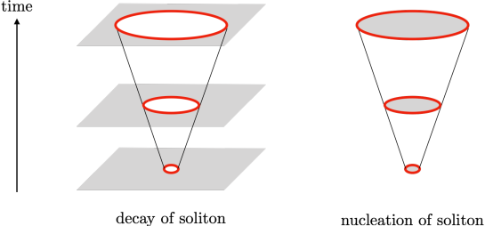
Figure 1: The schematic picture of the decay of soliton by nucleating a hole (left) and the creation of soliton by nucleating a disk soliton (right). Grey objects stands for the solitons and the red objects corresponds to the strings.

Here, we consider a disk of a soliton bounded by a string loop in the homogeneous vacuum. Let us consider the spatial dimension $d$, and later we will set $d=2,3$. In the thin-defect approximation, the bounce action reads

$$S(R)={\rm vol}(S^{d-1})R^{d-1}\mu+{\rm vol}(B^{d})R^{d}\sigma,$$ (3.9)

where $R$ is the radius of the soliton, and ${\rm vol}(S^{d-1})R^{d-1}$ and ${\rm vol}(B^{d})$ are volumes of the unit hypersphere and hyperball, given by

$${\rm vol}(S^{d-1})=\frac{2\pi^{\frac{d}{2}}}{\Gamma\left(\frac{d}{2}\right)},\qquad{\rm vol}(B^{d})=\frac{\pi^{d/2}}{\Gamma\left(\frac{d+2}{2}\right)},$$ (3.10)

respectively. Note that the string tension $\mu$ is not logarithmically divergent but a finite constant in the presence of the $U(1)$ breaking term (the third term in Eq. (3.7)). See Appendix A for some details.

Clearly, $\mu$ is always positive. In contrast, the soliton tension $\sigma$ given in Eq. (3.5) can be either positive or negative. In the absence of the topological term ($c=0$), $\sigma$ is positive, and $S$ has no stationary points except for $R=0$. Namely, quantum nucleation of the disk is prohibited.

However, the situation drastically changes in the presence of the topological term, $c\neq 0$, because the soliton tension can be negative $\sigma<0$ for $B>B_{\rm c}$. Then, a nontrivial stationary point exists at

$$R=\frac{d-1}{d}\frac{{\rm vol}(S^{d-1})}{{\rm vol}(B^{d})}\frac{\mu}{(-\sigma)}.$$ (3.11)

and the nucleation probability can be calculated as

$$P_{\text{nucleation}}=Ae^{-S},\quad S=\frac{(d-1)^{d-1}}{d^{d}}\frac{\left[{\rm vol}(S^{d-1})\right]^{d}}{\left[{\rm vol}(B^{d})\right]^{d-1}}\frac{\mu^{d}}{(-\sigma)^{d-1}}.$$ (3.12)

Since $-\sigma$ given in Eq. (3.5) is maximized at $\alpha=0$ ($\pi$) for $c>0$ ($<0$), the bounce action is minimized there with the negative soliton tension

$$\sigma_{\perp}=16mv^{2}\left(1-\frac{B}{B_{\rm c}}\right)<0.$$ (3.13)

Therefore, the nucleation probability is maximized for the soliton perpendicular to ${\bm{B}}$. Once the disk perpendicular to ${\bm{B}}$ is nucleated, it rapidly expands. The thin-defect approximation is justified for $R\gg\delta_{\rm dw}$. This can be rewritten as $\mu/(-\sigma_{\perp})\gg 1/m$.

3.3 Decay probability of a soliton in external fields in the thin-defect approximation

Here we consider quantum decay of a soliton in the external field. Consider an infinitely large flat soliton perpendicular to the external field under the external field larger than $B_{\rm c}$. The bounce action of a hole on a soliton can be written in the thin-defect limit as

$$S(R)={\rm vol}(S^{d-1})R^{d-1}\mu-{\rm vol}(B^{d})R^{d}\sigma_{0}\left(1-\frac{B}{B_{\rm c}}\right),$$ (3.14)

with $\sigma_{0}=16mv^{2}$. Since the second term is positive for $B>B_{\rm c}$, the bounce action does not have stationary point, and therefore the decay is prohibited. We should emphasized that the soliton which is metastable for $B=0$ is completely stable for $B>B_{\rm c}$.

On the other hand, when we instantaneously decrease $B$ below $B_{\rm c}$, the stationary point of the bounce action appears at

$$R=\frac{B_{\rm c}}{B_{\rm c}-B}\frac{d-1}{d}\frac{{\rm vol}(S^{d-1})}{{\rm vol}(B^{d})}\frac{\mu}{\sigma_{0}},$$ (3.15)

and the value of the action reads

$$S=\left(\frac{B_{\rm c}}{B_{\rm c}-B}\right)^{d-1}\frac{(d-1)^{d-1}}{d^{d}}\frac{\left[{\rm vol}(S^{d-1})\right]^{d}}{\left[{\rm vol}(B^{d})\right]^{d-1}}\frac{\mu^{d}}{\sigma_{0}^{d-1}}.$$ (3.16)

Comparing this with the bounce action without external field, we find

$$S\big{|}_{B=0}<S\big{|}_{0<B<B_{\rm c}}.$$ (3.17)

This implies that the decay rate of the soliton is suppressed by the external field. As the external field $B$ increases toward $B_{\rm c}$ from below, the action diverges and the quantum decay is strongly suppressed.

4 Numerical simulations for quantum nucleation of solitons

In this section, we numerically calculate nucleation probability of solitons. In Subsec. 4.1 we rewrite the Lagrangian in terms of dimensionless variables. In Subsecs. 4.2 and 4.3, we calculate nucleation probabilities of solitons by numerically constructing bounce solutions in 2+1 and 3+1 dimensions, respectively.

4.1 Preliminary

A great benefit of considering the linear sigma model in Eq. (3.7) is that we can treat the soliton and strings as regular objects of finite sizes. With them at hand we can go beyond the thin-defect limit.

We will numerically solve EOM of Lagrangian in Eq. (3.7). To this end, it is useful to rewrite Eq. (3.7) in terms of the dimensionless variables

$$\tilde{x}^{\mu}=mx,\quad\tilde{\phi}=v^{-1}\phi,\quad\tilde{\lambda}=\frac{m_{h}^{2}}{m^{2}},\quad\tilde{\bm{B}}=m^{-1}c{\bm{B}}.$$ (4.1)

Then, we have the Lagrangian

$${\cal L}_{\rm UV}=m^{2}v^{2}\left[|\tilde{\partial}_{\mu}\tilde{\phi}|^{2}-\frac{\tilde{\lambda}}{4}\left(|\tilde{\phi}|^{2}-1\right)^{2}+\tilde{\phi}+\tilde{\phi}^{*}+\tilde{\bm{j}}\cdot\tilde{\bm{B}}\right]$$ (4.2)

where $\tilde{\lambda}$ is the unique parameter characterizing solutions. For the (meta-)stable solitons and strings to exist, we need to assume $\tilde{\lambda}\gg 1$ corresponding to the condition in Eq. (2.2). For concreteness, we will assume that the soliton is perpendicular to the $z$-axis. Therefore, the last term in the bracket can be written as

$$\tilde{\bm{j}}\cdot\tilde{\bm{B}}=\tilde{B}\tilde{j}_{z}\cos\alpha.$$ (4.3)

The Hamiltonian reads

$${\cal H}_{\rm UV}=m^{2}v^{2}\tilde{\cal H}_{\rm UV},\quad\tilde{\cal H}_{\rm UV}=\left|\tilde{\nabla}\tilde{\phi}_{z}\right|^{2}+\frac{\tilde{\lambda}}{4}\left(|\tilde{\phi}|^{2}-1\right)^{2}-(\tilde{\phi}+\tilde{\phi}^{*})-\tilde{j}_{z}\tilde{B}\cos\alpha.$$ (4.4)

4.2 Quantum nucleation of a soliton in $2+1$ dimensions

Here, we investigate nucleation of solitons in $2+1$ dimensions, in which the soliton is a linear object and the vortex is a particle object. The $2+1$ dimensional version of Eq. (3.9) with $d=2$ is

$$S=2\pi R\mu+\pi R^{2}\sigma.$$ (4.5)

Its extremum is given by Eq. (3.12) for $d=2$,

$$R_{0}=\frac{\mu}{-\sigma},\qquad S_{0}=\frac{\pi\mu^{2}}{-\sigma}.$$ (4.6)

Note that we have $[v]=\frac{1}{2}$, $[\lambda]=1$, and $[m]=1$ in $2+1$ dimensions. We will compare this analytic formula in the thin-defect limit with numerical simulations for the soliton with finite thickness.

Once we obtain a numerical solution for a soliton attached by a vortex and an anti-vortex at its both ends, we can measure the dimensionless radius $\tilde{R}$ (a half length) of the soliton and evaluate the dimensionless total energy $\tilde{\cal E}$ by

$$\tilde{\cal E}(\tilde{R})=\int d^{2}\tilde{x}\ \tilde{\cal H}_{\rm UV}(\tilde{R}).$$ (4.7)

From this, we can evaluate the bounce action through the following formula

$$S=\int d^{3}x\,{\cal H}_{\rm UV}=\frac{v^{2}}{m}\int d^{3}\tilde{x}\,\tilde{\cal H}_{\rm UV}=\alpha_{1}\frac{v^{2}}{m}\int_{0}^{\tilde{R}}d\tilde{r}~{}\tilde{\cal E}(\tilde{r}),$$ (4.8)

with a constant $\alpha_{1}=\pi$ (see Appendix B for a derivation). To understand the formula quickly, let us substitute the energy formula $\tilde{\cal E}(\tilde{R})=2\tilde{\mu}+2\tilde{R}\tilde{\sigma}$ with $\tilde{\mu}=\mu/v^{2}$ and $\tilde{\sigma}=\sigma/(mv^{2})$ in the thin-defect limit (the soliton of the length $2\tilde{R}$ with two vortices). We easily find that the bounce action in Eq. (4.5) is correctly reproduced.

Note that the formula in Eq. (4.8) is valid only for constant $\mu$. If $\mu$ depended on $R$ logarithmically as the usual global vortex, we cannot use Eq. (4.8). In Appendix A, we show our numerical solution in which the profile of the scalar field exponentially converges to the VEV in the asymptotic region, in contrast to the usual global vortex without any domain walls for which the profiles polynomially approaches to the VEV.

By differentiating $S$ by $R$, we have

$$\frac{dS}{dR}=\alpha_{1}\frac{v^{2}}{m}\frac{d\tilde{R}}{dR}\tilde{\cal E}(\tilde{R})=\alpha_{1}v^{2}\tilde{\cal E}(\tilde{R}).$$ (4.9)

The extremum of $S$ is then identified with the zero of ${\cal E}$:

$$\frac{dS}{dR}=0\quad\Leftrightarrow\quad\tilde{\cal E}(\tilde{R})=0.$$ (4.10)

The remaining task is constructing suitable numerical configurations with a soliton bounded by a vortex and an anti-vortex. To this end, we use the standard relaxation scheme. Our method consists of two steps. Firstly, we take a product ansatz of a pair of a vortex and an anti-vortex separated at distance $2\tilde{R}_{\rm ini}$ as an initial configuration of the relaxation. At this stage, we fix the positions of the vortices. Then, the straight soliton of the length $2\tilde{R}_{\rm ini}$ is generated and the configuration converges quite soon. We use this convergent configuration as the initial configuration for the second relaxation, in which we do not fix the vortex positions. During the second relaxation process, the vortices approach to each other due to the soliton tension, and eventually annihilate each other. We repeatedly measure the distance $2\tilde{R}$ of the vortices and compute $\tilde{\cal E}(\tilde{R})$.

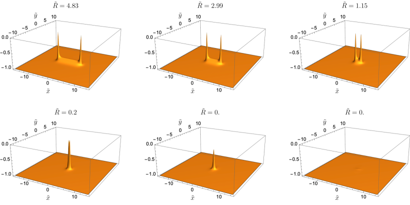
Figure 2: The soliton attached by a vortex and anti-vortex in $2+1$ dimensions. The negative amplitude $(-|\tilde{\phi}|)$ is plotted.

To be concrete, we take $\tilde{\lambda}=100$ which is large enough for the soliton and vortices to be classically metastable. The amplitudes $(-|\tilde{\phi}|)$ for several different separations are shown in Fig. 2. The two peaks correspond to the vortex and anti-vortex while the linear object stretching between them is the soliton which is visible only for a large $\tilde{R}$. We evaluate $\tilde{\cal E}$ with three different values of $\tilde{B}\cos\alpha=\{1,1/2,1/4\}$ in Eq. (4.4).

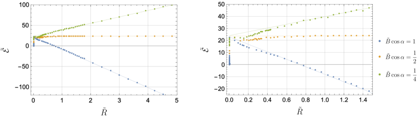
Figure 3: The dimensionless total energy $\tilde{\cal E}$ is plotted as the function of the dimensionless radius $\tilde{R}$. Three different choices of $\tilde{B}\cos\alpha=\{1,1/2,1/4\}$ corresponding to $B\geq B_{c}$, $B=B_{c}$ and $B\leq B_{c}$, respectively, are shown. The right panel is the zoom-up around $\tilde{R}=0$ of the left one.

The results are shown in Fig. 3. The datas are well fitted by a linear function in the large $\tilde{R}$ region

$$\tilde{\cal E}=2\tilde{R}a+2b,$$ (4.11)

which should be compared with the thin-defect limit $\tilde{\cal E}=2\tilde{R}\tilde{\sigma}+2\tilde{\mu}$. The coefficient $a$ can be either positive or negative because it is related to the soliton tension which depends on $\tilde{B}\cos\alpha$. On the other hand, the constant $b$ should be insensitive on $\tilde{B}\cos\alpha$ because it should be identified with the vortex tension which is independent on the background field. Indeed, our numerical solutions show that the three lines almost meet at $\tilde{R}=0$ in Fig. 3. The coefficients read numerically are shown in Table.1. Thus we numerically determine the tensions $\tilde{\mu}$ and $\tilde{\sigma}$. Importantly, $\tilde{\mu}$ is a constant as we mentioned above, see also Appendix A.

$\tilde{B}\cos\alpha~{}(d=2)$	$a(\sim\tilde{\sigma})$	$b(\sim\tilde{\mu})$
$1$	$-15.6$	$11.6$
$1/2$	$0.07$	$12.0$
$1/4$	$7.85$	$12.2$

$\tilde{B}\cos\alpha~{}(d=3)$	$a(\sim\tilde{\sigma})$	$b(\sim\tilde{\mu})$	$c$
$1$	$-15.3$	$11.8$	$45.6$
$1/2$	$-0.15$	$12.7$	$28.4$
$1/4$	$7.78$	$12.3$	$24.3$

Table 1: The numerically obtained coefficients in Eqs. (4.11) and (4.17).

Among the three different choices, only $\tilde{B}\cos\alpha=1$ leads to the negative soliton tension, corresponding to the case of $B\geq B_{c}$. The stationary point is $\tilde{R}_{0}\simeq 0.75$, and the value of the bounce action is about $\tilde{S}\simeq b\tilde{R}\simeq 9.0$. Hence, the nucleation probability can be estimated as

$$P_{\rm nucleation}=A\exp\left(-\alpha_{1}\frac{v^{2}}{m}\times 9.0\right).$$ (4.12)

Note that the numerically determined values $(\tilde{R}_{0},\tilde{\sigma},\tilde{\mu})=(0.75,-15.6,11.6)$ is consistent with the analytic formula $\tilde{R}_{0}=\tilde{\mu}/(-\tilde{\sigma})$ for the thin-defect limit.

4.3 Quantum nucleation of a soliton in $3+1$ dimensions

Next, we numerically investigate quantum nucleation of a disk soliton bounded by a string loop in $3+1$ dimensions. By putting $d=3$ in Eq. (3.9), the bounce action of the thin-defect limit is given by

$$S=\pi R^{2}\mu+\frac{4\pi}{3}R^{3}\sigma,$$ (4.13)

and its extremum is given by Eq. (3.12) for $d=3$,

$$R_{0}=\frac{2\mu}{-\sigma},\qquad S_{0}=\frac{16\pi\mu^{3}}{3\sigma^{2}}.$$ (4.14)

The numerical procedures we adopt in this subsection are the same as those in the previous subsection except for differences due to the spacial dimensions. We numerically evaluate the dimensionless mass $\tilde{\cal E}$ for a disk of a soliton of the radius $R$

$$\tilde{\cal E}(\tilde{R})=\int d^{3}\tilde{x}~{}\tilde{\cal H}_{\rm UV},$$ (4.15)

where the dimensionless Hamiltonian $\tilde{\cal H}_{\rm UV}$ is given in Eq. (4.4). Then, we evaluate the bounce action $S$ by the following formula

$$S(R)=\int d^{4}x\,{\cal H}_{\rm UV}=\frac{v^{2}}{m^{2}}\int d^{4}\tilde{x}\,\tilde{\cal H}_{\rm UV}=\alpha_{2}\frac{v^{2}}{m^{2}}\int_{0}^{\tilde{R}}d\tilde{r}~{}\tilde{\cal E}(\tilde{r}).$$ (4.16)

The constant factor is $\alpha_{2}=4$ whose derivation is given in Appendix B. Again, we should note that this formula is valid for the constant $\mu$. As a quick check of the formula, one can reproduce Eq. (4.13) by substituting $\tilde{\cal E}=2\pi\tilde{R}\tilde{\mu}+\pi\tilde{R}^{2}\tilde{\sigma}$.

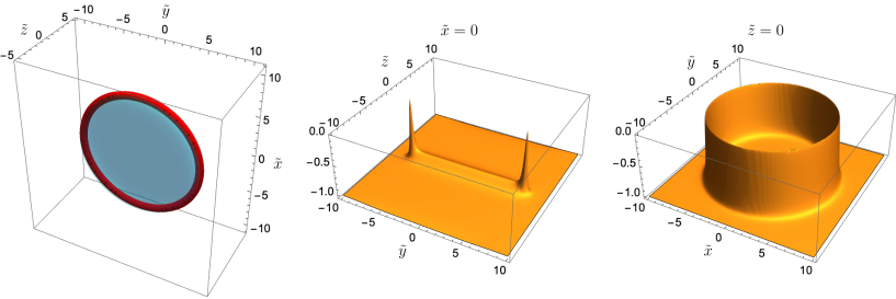
Figure 4: The three-dimensional disk soliton perpendicular to the $z$-axis generated from the two-dimensional linear soliton. In the left panel the red part shows the region for $|\tilde{\phi}|<0.9$, and the blurred-blue part corresponds to the region for ${\rm Re}[\tilde{\phi}]<0.4$. The middle and right panels show $-|\tilde{\phi}|$ on the $\tilde{x}=0$ and $\tilde{z}=0$ cross sections, respectively.

As before we take relatively large value $\tilde{\lambda}=100$ to assure the classical stability of the solitons and strings. In order to prepare a disk shape soliton, we recycle the numerical configuration of the linear soliton attached by two vortices in $2+1$ dimensions. Set the two-dimensional linear soliton along the $x$-axis on the $xz$-plane, and let $\phi_{\rm 2d}(x,z)$ be the corresponding field configuration. Then, a three-dimensional disk soliton perpendicular to the $z$-axis can be obtained by rotating it around the $z$-axis, namely $\phi_{\rm 3d}(x,y,z)=\phi_{\rm 2d}(x\cos\theta+y\sin\theta,z)$ with $\tan\theta=y/x$, see Fig. 4.

Having this as an initial configuration, we evolve it by a standard relaxation method. The disk soliton shrinks as the relaxation process proceeds. We measure the radius and the mass, so that we determine the function $\tilde{\cal E}(\tilde{R})$. Finally, we calculate the bounce action $S(R)$ by plugging it to the formula in Eq. (4.16).

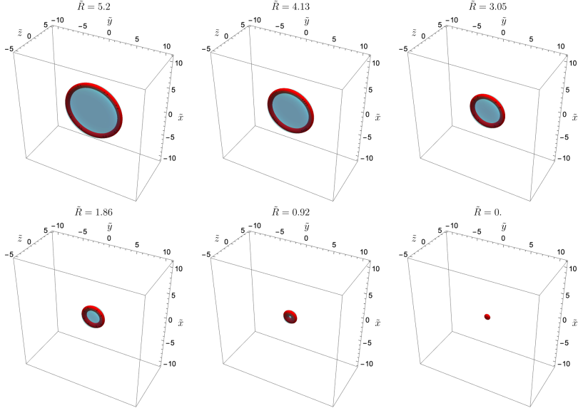
Figure 5: The disk soliton bounded by a ring string. The red part shows the region for $|\tilde{\phi}|<0.9$, and the blurred-blue part corresponds to the region for ${\rm Re}[\tilde{\phi}]<0.4$.

The time evolution of the disk soliton under the relaxation process is shown in Fig. 5. The disk is initially large, and we can clearly observe a circular closed string (red part: $|\tilde{\phi}|<0.9$) and a disk soliton (blurred-blue part: ${\rm Re}[\tilde{\phi}]<0.4$). We determine the radius $\tilde{R}$ of the ring by seeking the point where $|\tilde{\phi}|=0$. Note that the energy does not immediately vanishes when $\tilde{R}$ reaches zero. This is a finite width effect which is missed in the thin-defect limit. Since the soliton and string are regular objects with finite sizes, a remnant of energy still exists and it gradually decays and finally disappears.

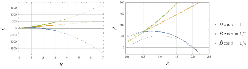
Figure 6: The dimensionless total energy $\tilde{\cal E}$ is plotted as the function of the dimensionless radius $\tilde{R}$ for $d=3$. We set $\tilde{B}\cos\alpha=\{1,1/2,1/4\}$. The right panel is the zoom-up near $\tilde{R}=0$ of the left one.

The numerical results for $\tilde{B}\cos\alpha=\{1,1/2,1/4\}$ are shown in Fig. 6. The fact that the energy of $\tilde{B}\cos\alpha=1$ is negative for large $\tilde{R}$ indicates that the soliton tension is negative. The zero of $\tilde{\cal E}$ is found as $\tilde{R}\simeq 2$ which should correspond to the extremum point of the bounce action. The energy of $\tilde{B}\cos\alpha=1/2$ is approximately a linear function of $\tilde{R}$ implying the soliton tension vanishes. That of $\tilde{B}\cos\alpha=1/4$ grows faster than linear functions, implying that the soliton tension is positive. These are well fitted by

$$\tilde{\cal E}=\pi\tilde{R}^{2}a+2\pi\tilde{R}b+c.$$ (4.17)

The values of these coefficients are shown in Table 1. The values of $a$ ($\sim\tilde{\sigma}$) and $b$ ($\sim\tilde{\mu}$) are consistent between the left ($d=2$) and right ($d=3$) tables in Table 1. The last term $c$ corresponds to the remnant energy at $\tilde{R}=0$. This is absent in the thin-defect limit. Hence, the bounce action for the finite size soliton is slightly larger than the one at the thin-defect limit.

By using the fit in Eq. (4.17), we can evaluate the action for $\tilde{B}\cos\alpha=1$ as

$$S=\alpha_{2}\frac{v^{2}}{m^{2}}\int_{0}^{\tilde{R}_{0}=2}d\tilde{r}~{}\tilde{\cal E}(\tilde{r})\simeq 111\alpha_{2}\frac{v^{2}}{m^{2}}.$$ (4.18)

Thus, the nucleation probability can be obtained as

$$P_{\rm nucleation}=A\exp\left(-111\alpha_{2}\frac{v^{2}}{m^{2}}\right).$$ (4.19)

Before closing this section, let us examine the relevance of the remnant energy found above. If we fit the numerical data by ignoring the remnant energy with forcing $c=0$, then we find $a=-16.7$ and $b=16.7$, see the red-dashed curve in Fig. 6. The value of integration for the constrained fit is $\int_{0}^{\tilde{R}_{0}=2}d\tilde{r}~{}\tilde{\cal E}\simeq 69$, so that the nucleation probability is slightly increased. Here, $a=-16.7$ is still consistent with the one obtained in the $d=2$ case, whereas $b=16.7$ shows a relatively large discrepancy from $b$ in the $d=2$ case. Hence, the string tension $b$ is not correctly captured by the constrained fit. Thus, we conclude that the remnant energy $c$ included in the unconstrained fit is not a sort of artifacts of the numerical simulation but it should be considered as a real finite width effect.

In conclusion, we have succeeded in numerically evaluating the bounce action for the soliton bounded by the string with finite thickness. The finite width effect has been found and it slightly reduces the nucleation probability compared with the thin-defect limit.

5 Summary and discussion

We have proposed quantum nucleation of topological solitons through quantum tunneling, as a novel mechanism for formation of topological solitons. We have discussed chiral solitons in a complex $\phi^{4}$ model (an axion model) with a topological term, which is a low-energy theory of chiral magnets with an easy-plane anisotropy and QCD at finite density under strong magnetic field or rapid rotation. First, we have estimated the creation probability analytically in terms of tensions of string (vortex) and soliton in the thin-defect approximation in any dimension. Second, we have performed numerical simulations in $2+1$ and $3+1$ dimensions by the relaxation (gradient flow) method, and have obtained creation probabilities. We have found a good agreement between the thin-defect approximation and direct numerical simulation in $2+1$ dimensions and have found, in $3+1$ dimensions, a difference between them at short distances at the subleading order, which can be interpreted as the remnant energy.

We have considered the complex $\phi^{4}$ model as an UV theory for the sine-Gordon model at IR limit appearing in various context. Sine-Gordon solitons are almost insensitive to UV, but different UV theories give different structures of strings (vortices). However, creation probabilities will be insensitive to such details.

In this study, we have estimated the nucleation probability in the vacuum where there are no solitons. In the case with the external field above the critical value, the true ground state is a CSL. Formation of the CSL in the homogeneous vacuum should occur in the following process. Let us turn on the external field $B>B_{\rm c}$ in the homogeneous vacuum. Initially, disk solitons of the critical radius $R_{0}$ in Eq. (4.14) are nucleated all over with the creation rate in Eq. (4.19). They rapidly expand as in the right panel of Fig. 1, growing up to infinitely large solitons. These solitons repel each other and thus adjust intersoliton distances to minimize the total energy, thereby eventually forming into a CSL as schematically shown in Fig. 7.

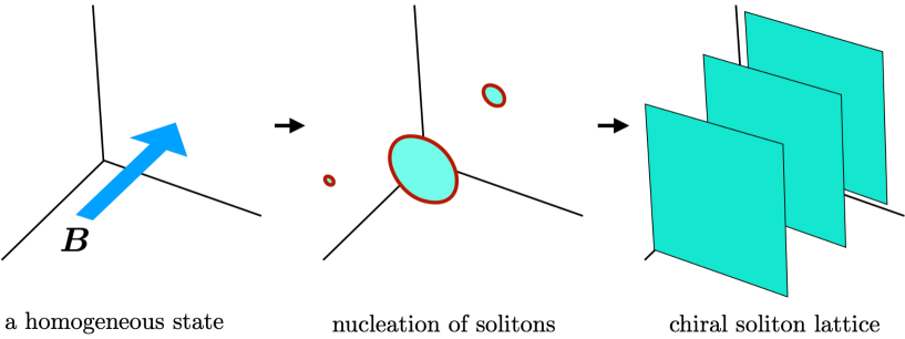
Figure 7: Nucleation of solitons and formation of a CSL.

Of course, this is a rough sketch and we need more detailed analysis of dynamical process. We also need to calculate nucleation probabilities of solitons not in the homogeneous vacuum but also in inhomogeneous soliton backgrounds. For instance, once the CSL ground state is formed, nucleation probabilities of solitons should be zero in such a background. If we instantaneously increase (decrease) the external field in the CSL ground state, the number density of solitons should be decreased (increased). We thus need nucleation (decay) rates of solitons in the CSL background, which remain as a future work.

In this paper, we have considered the Abelian sine-Gordon model for simplicity. On the other hand, it was found in Ref. Eto:2021gyy that in the case of two-flavor baryonic matter under rotation, non-Abelian solitons with non-Abelian ${\mathbb{C}}P^{N-1}$ moduli Nitta:2014rxa ; Eto:2015uqa are also present in the ground state of QCD in a certain parameter region. In this case, a non-Abelian soliton is bounded by a non-Abelian global string Nitta:2014rxa ; Eto:2021nle . In such a case, the creation probability may depend on the dimension $N$ of the moduli as numerical factor.

In $2+1$ dimensions, the pseudo-NG mode is mapped to an electromagnetic field under a duality, while vortices are mapped to charged particles. With nonzero mass $m$, particles are confined by electric fluxes. In this duality, the topological term will be mapped to a constant electric field. It remains as a future problem to study nucleation probabilities in terms of the duality. In $2+1$ dimensions, there is a BKT transition at finite temperature. It is interesting to discuss whether there is any conflict between quantum nucleation and the BKT transition.

Note added: While this paper is being completed, we were informed that the authors of Ref. Nishimura was preparing a draft which may have some overlap with our work.

Appendix A Asymptotic behavior of the scalar field of a vortex attached by a soliton

Here, we show a numerical solution with some more details to demonstrate that the amplitude of $\phi$ for a vortex attached by a soliton decays exponentially fast, in contrast to the slow-tail with a negative power of isolated global vortices without solitons. For this purpose, we use a configuration of a vortex and an anti-vortex connected by a soliton discussed in Sec. 4.2, see Fig. 2. When the vortex and anti-vortex are well separated compared with the width of the soliton, the configuration around the vortex is close to that of a single vortex attached by a soliton.

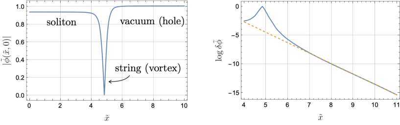
Figure 8: The left panel shows $\tilde{\phi}(\tilde{x},0)$ for the configuration shown in the top-left panel of Fig. 2, and the right panel shows asymptotic behavior of the same solution.

The left panel of Fig. 8 shows a scalar field profile $\tilde{\phi}(\tilde{x},0)$ at a cross section $y=0$ of the configuration shown in the top-left panel of Fig. 2 with $\tilde{R}=4.83$. One can see that apart from the vortex core, the scalar field $\tilde{\phi}$ quickly converges to a constant in the vacuum. To confirm that the asymptotic behavior is an exponential tail, we show $\log\delta\tilde{\phi}=\log(\tilde{v}-|\tilde{\phi}|)$ in the right panel of Fig. 8. We numerically fit the asymptotic tail and the result is $\delta\tilde{\phi}(\tilde{x},0)\propto e^{-1.8\tilde{x}}$. Thus, the amplitude converges exponentially fast to the VEV.

We can confirm the same behaviors in any directions from the vortex center except for the directions of the soliton within its width. This fact implies that the vortex tension is finite as in Eq. (2.7), in contrast to an isolated global vortex whose tension is logarithmically divergent as in Eq. (2.3). Physically, the logarithmically divergent behavior (of an isolated global vortex) is replaced by the soliton tension. This point was missed in the literature Preskill:1992ck ; Vilenkin:2000jqa in which the vortex tension was assumed to be logarithmically divergent even when the vortex is attached by a soliton. This is crucial to evaluate bounce actions in the thin-defect limit and likewise the decay rates and nucleation probabilities of topological solitons.

Appendix B A derivation of Eqs. (4.8) and (4.16)

In this appendix, we give a derivation of Eqs. (4.8) and (4.16) for the spatial dimension $d=2,3$. However, we will consider generic $d$ below. Since the number of codimensions of strings(vortices) is 2 and that of solitons is 1, a soliton is a $(d-1)$-dimensional ball $B^{d-1}$ while the string wrapping the soliton is a $(d-2)$-dimensional sphere $S^{d-2}$. The volumes of unit $d$-sphere and $d$-ball are given by

$${\rm vol}(S^{d-1})=\frac{2\pi^{\frac{d}{2}}}{\Gamma\left(\frac{d}{2}\right)},\qquad{\rm vol}(B^{d})=\frac{\pi^{d/2}}{\Gamma\left(\frac{d+2}{2}\right)}.$$ (B.1)

Therefore, the mass in the thin-defect limit reads

$$\tilde{\cal E}(\tilde{R})=\int d^{d}\tilde{x}\,\tilde{\cal H}_{\rm UV}={\rm vol}(S^{d-2})\tilde{R}^{d-2}\tilde{\mu}+{\rm vol}(B^{d-1})\tilde{R}^{d-1}\tilde{\sigma},$$ (B.2)

with the dimensionless tensions of string and soliton

$$\tilde{\mu}=\mu/v^{2},\quad\tilde{\sigma}=\sigma/(mv^{2}),$$ (B.3)

respectively. On the other hand, the string world-volume is $S^{d-1}$ and the soliton world-volume is $B^{d-1}$ for the bounce action, and we have

$$\tilde{S}(\tilde{R})\equiv\int d^{d+1}\tilde{x}\,\tilde{\cal H}_{\rm UV}={\rm vol}(S^{d-1})\tilde{R}^{d-1}\tilde{\mu}+{\rm vol}(B^{d})\tilde{R}^{d}\tilde{\sigma}.$$ (B.4)

Integrating $\tilde{\cal E}(\tilde{R})$, we find

$$\int^{\tilde{R}}_{0}d\tilde{r}~{}\tilde{\cal E}(\tilde{r}) = \frac{1}{d-1}{\rm vol}(S^{d-2})\tilde{R}^{d-1}\mu+\frac{1}{d}{\rm vol}(B^{d-1})\tilde{R}^{d}\sigma$$ (B.5)

$$= \left(\frac{1}{d-1}\frac{{\rm vol}(S^{d-2})}{{\rm vol}(S^{d-1})}\right){\rm vol}(S^{d-1})\tilde{R}^{d-1}\mu+\left(\frac{1}{d}\frac{{\rm vol}(B^{d-1})}{{\rm vol}(B^{d})}\right){\rm vol}(B^{d})\tilde{R}^{d}\sigma.\;\;\;$$

Note that the two ratios are identical as

$$\alpha_{d-1}\equiv(d-1)\frac{{\rm vol}(S^{d-1})}{{\rm vol}(S^{d-2})}=d\frac{{\rm vol}(B^{d})}{{\rm vol}(B^{d-1})},$$ (B.6)

and therefore we have

$$\tilde{S}(\tilde{R})=\alpha_{d-1}\int^{\tilde{R}}_{0}d\tilde{r}~{}\tilde{\cal E}(\tilde{r}).$$ (B.7)

We assume that this formula is valid not only for the thin-defect limit but also the case that the defects have regular sizes. We have used $\alpha_{1}=\pi$ and $\alpha_{2}=4$ in the text.

References

- (1) R. Rajaraman, Solitons and Instantons: An Introduction to Solitons and Instantons in Quantum Field Theory, North-Holland Personal Library (1987).
- (2) V.A. Rubakov, Classical theory of gauge fields, Princeton University Press, Princeton, New Jersey (5, 2002).
- (3) N.S. Manton and P. Sutcliffe, Topological solitons, Cambridge Monographs on Mathematical Physics, Cambridge University Press (2004), 10.1017/CBO9780511617034.
- (4) Y.M. Shnir, Magnetic Monopoles, Text and Monographs in Physics, Springer, Berlin/Heidelberg (2005), 10.1007/3-540-29082-6.
- (5) T. Vachaspati, Kinks and domain walls: An introduction to classical and quantum solitons, Cambridge University Press (4, 2010), 10.1017/CBO9780511535192.
- (6) M. Dunajski, Solitons, instantons, and twistors, Oxford Graduate Texts In Mathematics, Oxford University Press, U.S.A. (2010).
- (7) E.J. Weinberg, Classical solutions in quantum field theory: Solitons and Instantons in High Energy Physics, Cambridge Monographs on Mathematical Physics, Cambridge University Press (9, 2012), 10.1017/CBO9781139017787.
- (8) Y.M. Shnir, Topological and Non-Topological Solitons in Scalar Field Theories, Cambridge University Press (7, 2018), 10.1017/9781108555623.
- (9) D. Tong, TASI lectures on solitons: Instantons, monopoles, vortices and kinks, in Theoretical Advanced Study Institute in Elementary Particle Physics: Many Dimensions of String Theory, 6, 2005 [hep-th/0509216].
- (10) D. Tong, Quantum Vortex Strings: A Review, Annals Phys. 324 (2009) 30 [0809.5060].
- (11) M. Eto, Y. Isozumi, M. Nitta, K. Ohashi and N. Sakai, Solitons in the Higgs phase: The Moduli matrix approach, J. Phys. A 39 (2006) R315 [hep-th/0602170].
- (12) M. Shifman and A. Yung, Supersymmetric Solitons and How They Help Us Understand Non-Abelian Gauge Theories, Rev. Mod. Phys. 79 (2007) 1139 [hep-th/0703267].
- (13) M. Shifman and A. Yung, Supersymmetric solitons, Cambridge Monographs on Mathematical Physics, Cambridge University Press (5, 2009), 10.1017/CBO9780511575693.
- (14) M. Eto, Y. Hirono, M. Nitta and S. Yasui, Vortices and Other Topological Solitons in Dense Quark Matter, PTEP 2014 (2014) 012D01 [1308.1535].
- (15) T.W.B. Kibble, Topology of Cosmic Domains and Strings, J. Phys. A 9 (1976) 1387.
- (16) T.W.B. Kibble, Some Implications of a Cosmological Phase Transition, Phys. Rept. 67 (1980) 183.
- (17) A. Vilenkin, Cosmic Strings and Domain Walls, Phys. Rept. 121 (1985) 263.
- (18) M. Hindmarsh and T. Kibble, Cosmic strings, Rept. Prog. Phys. 58 (1995) 477 [hep-ph/9411342].
- (19) T. Vachaspati, L. Pogosian and D. Steer, Cosmic Strings, Scholarpedia 10 (2015) 31682 [1506.04039].
- (20) A. Vilenkin and E.S. Shellard, Cosmic Strings and Other Topological Defects, Cambridge University Press (7, 2000).
- (21) N.D. Mermin, The topological theory of defects in ordered media, Rev. Mod. Phys. 51 (1979) 591.
- (22) G.E. Volovik, The Universe in a helium droplet, International Series of Monographs on Physics, Oxford Scholarship Online (2009), 10.1093/acprof:oso/9780199564842.001.0001.
- (23) B.V. Svistunov, E.S. Babaev and N.V. Prokof’ev, Superfluid States of Matter, Cambridge Monographs on Mathematical Physics, CRC Press (2015), 10.1201/b18346.
- (24) G. Blatter, M.V. Feigel’man, V.B. Geshkenbein, A.I. Larkin and V.M. Vinokur, Vortices in high-temperature superconductors, Rev. Mod. Phys. 66 (1994) 1125.
- (25) T. Giamarchi and S. Bhattacharya, Vortex phases, In: Berthier, C., Lévy, L.P., Martinez, G. (eds) High Magnetic Fields., Lecture Notes in Physics, Springer, Berlin, Heidelberg (2002), [arXiv:cond-mat/0111052 [cond-mat.supr-con]].
- (26) A.V. Ustinov, Solitons in Josephson Junctions: Physics of Magnetic Fluxons in Superconducting Junctions and Arrays, Wiley-VCH (2015).
- (27) Y. Kawaguchi and M. Ueda, Spinor Bose-Einstein condensates, Phys. Rept. 520 (2012) 253.
- (28) L. Pismen, Vortices in Nonlinear Fields: From Liquid Crystals to Superfluids, from Non-Equilibrium Patterns to Cosmic Strings, International Series of Monographs on Physics, Clarendon Press (1999).
- (29) Y.M. Bunkov and H. Godfrin, Topological Defects and the Non-Equilibrium Dynamics of Symmetry Breaking Phase Transitions (NATO Science Series), Springer, Dordrecht (2000), 10.1007/978-94-011-4106-2.
- (30) N. Nagaosa and Y. Tokura, Topological properties and dynamics of magnetic skyrmions, Nature Nanotech 8 (2013) 899–911.
- (31) B. Göbel, I. Mertig and O.A. Tretiakov, Beyond skyrmions: Review and perspectives of alternative magnetic quasiparticles, Phys. Rept. 895 (2021) 1 [2005.01390].
- (32) W.H. Zurek, Cosmological Experiments in Superfluid Helium?, Nature 317 (1985) 505.
- (33) W.H. Zurek, Cosmological experiments in condensed matter systems, Phys. Rept. 276 (1996) 177 [cond-mat/9607135].
- (34) M.J. Bowick, L. Chandar, E.A. Schiff and A.M. Srivastava, The Cosmological Kibble mechanism in the laboratory: String formation in liquid crystals, Science 263 (1994) 943 [hep-ph/9208233].
- (35) P. Hendry, N. Lawson, R. Lee, P. Mcclintock and C. Williams, Generation of defects in superfluid 4he as an analogue of the formation of cosmic strings, Nature (1994) 315.
- (36) C. Baeuerle, Y.M. Bunkov, S.N. Fisher, H. Godfrin and G.R. Pickett, Laboratory simulation of cosmic string formation in the early Universe using superfluid He-3, Nature 382 (1996) 332.
- (37) V.M.H. Ruutu, V.B. Eltsov, A.J. Gill, T.W.B. Kibble, M. Krusius, Y.G. Makhlin et al., Big bang simulation in superfluid He-3-b: Vortex nucleation in neutron irradiated superflow, Nature 382 (1996) 334 [cond-mat/9512117].
- (38) L. Sadler, J. Higbie, S. Leslie, M. Vengalattore and D. Stamper-Kurn, Spontaneous symmetry breaking in a quenched ferromagnetic spinor bose-einstein condensate, Nature 443 (2006) 312.
- (39) C.N. Weiler, T.W. Neely, D.R. Scherer, A.S. Bradley and M.J.D. et al., Spontaneous vortices in the formation of bose-einstein condensates, Nature 455 (2008) 948.
- (40) V.L. Berezinsky, Destruction of long range order in one-dimensional and two-dimensional systems having a continuous symmetry group. I. Classical systems, Sov. Phys. JETP 32 (1971) 493.
- (41) V.L. Berezinsky, Destruction of long range order in one-dimensional and two-dimensional systems having a continuous symmetry group. II. Quantum systems, Sov. Phys. JETP 34 (1972) 610.
- (42) J.M. Kosterlitz and D.J. Thouless, Ordering, metastability and phase transitions in two-dimensional systems, J. Phys. C 5 (1972) L124.
- (43) J.M. Kosterlitz and D.J. Thouless, Ordering, metastability and phase transitions in two-dimensional systems, J. Phys. C 6 (1973) 1181.
- (44) M. Kobayashi, M. Eto and M. Nitta, Berezinskii-Kosterlitz-Thouless Transition of Two-Component Bose Mixtures with Intercomponent Josephson Coupling, Phys. Rev. Lett. 123 (2019) 075303 [1802.08763].
- (45) M. Kobayashi, G. Fejős, C. Chatterjee and M. Nitta, Vortex confinement transitions in the modified Goldstone model, Phys. Rev. Res. 2 (2020) 013081 [1908.11087].
- (46) D.J. Bishop and J.D. Reppy, Study of the superfluid transition in two-dimensional films, Phys. Rev. Lett. 40 (1978) 1727.
- (47) M.R. Beasley, J.E. Mooij and T.P. Orlando, Possibility of vortex-antivortex pair dissociation in two-dimensional superconductors, Phys. Rev. Lett. 42 (1979) 1165.
- (48) Z. Hadzibabic, P. Krüger and M.e.a. Cheneau.
- (49) S.W. Hawking, I.G. Moss and J.M. Stewart, Bubble Collisions in the Very Early Universe, Phys. Rev. D 26 (1982) 2681.
- (50) E.J. Copeland and P.M. Saffin, Bubble collisions in Abelian gauge theories and the geodesic rule, Phys. Rev. D 54 (1996) 6088 [hep-ph/9604231].
- (51) S. Digal and A.M. Srivastava, Formation of topological defects with explicit symmetry breaking, Phys. Rev. Lett. 76 (1996) 583 [hep-ph/9509263].
- (52) I.K. Affleck and N.S. Manton, Monopole Pair Production in a Magnetic Field, Nucl. Phys. B 194 (1982) 38.
- (53) I.K. Affleck, O. Alvarez and N.S. Manton, Pair Production at Strong Coupling in Weak External Fields, Nucl. Phys. B 197 (1982) 509.
- (54) A. Sen, Tachyon dynamics in open string theory, Int. J. Mod. Phys. A 20 (2005) 5513 [hep-th/0410103].
- (55) D.I. Bradley, S.N. Fisher, A.M. Guenault, R.P. Haley, J. Kopu, H. Martin et al., Relic topological defects from brane annihilation simulated in superfluid He-3, Nature Phys. 4 (2008) 46.
- (56) H. Takeuchi, K. Kasamatsu, M. Tsubota and M. Nitta, Tachyon Condensation Due to Domain-Wall Annihilation in Bose-Einstein Condensates, Phys. Rev. Lett. 109 (2012) 245301 [1205.2330].
- (57) M. Nitta, K. Kasamatsu, M. Tsubota and H. Takeuchi, Creating vortons and three-dimensional skyrmions from domain wall annihilation with stretched vortices in Bose-Einstein condensates, Phys. Rev. A 85 (2012) 053639 [1203.4896].
- (58) H. Takeuchi, K. Kasamatsu, M. Tsubota and M. Nitta, Tachyon Condensation and Brane Annihilation in Bose-Einstein Condensates: Spontaneous Symmetry Breaking in Restricted Lower-dimensional Subspace, J. Low Temp. Phys. 171 (2013) 443 [1211.3952].
- (59) P. De Gennes, Calcul de la distorsion d’une structure cholesterique par un champ magnetique, Solid State Communications 6 (1968) 163.
- (60) Y. Togawa, T. Koyama, K. Takayanagi, S. Mori, Y. Kousaka, J. Akimitsu et al., Chiral magnetic soliton lattice on a chiral helimagnet, Physical review letters 108 (2012) 107202.
- (61) Y. Togawa, Y. Kousaka, K. Inoue and J.-i. Kishine, Symmetry, structure, and dynamics of monoaxial chiral magnets, Journal of the Physical Society of Japan 85 (2016) 112001.
- (62) J.-i. Kishine and A.S. Ovchinnikov, Chapter one - theory of monoaxial chiral helimagnet, vol. 66 of Solid State Physics, pp. 1–130, Academic Press (2015), DOI.
- (63) A.A. Tereshchenko, A.S. Ovchinnikov, I. Proskurin, E.V. Sinitsyn and J.-i. Kishine, Theory of magnetoelastic resonance in a monoaxial chiral helimagnet, Phys. Rev. B 97 (2018) 184303.
- (64) J. Chovan, N. Papanicolaou and S. Komineas, Intermediate phase in the spiral antiferromagnet , Phys. Rev. B 65 (2002) 064433.
- (65) C. Ross and M. Sakai, N.and Nitta, Exact ground states and domain walls in one dimensional chiral magnets, JHEP 12 (2021) 163 [2012.08800].
- (66) I. Dzyaloshinskii, A Thermodynamic Theory of ‘Weak’ Ferromagnetism of Antiferromagnetics, J. Phys. Chem. Solids 4 (1958) 241.
- (67) T. Moriya, Anisotropic Superexchange Interaction and Weak Ferromagnetism, Phys. Rev. 120 (1960) 91.
- (68) A. Bogdanov and D. Yablonskii, Thermodynamically stable vortices in magnetically ordered crystals. The mixed state of magnets, Sov. Phys. JETP 68 (1989) 101.
- (69) A. Bogdanov, New localized solutions of the nonlinear field equations, JETP Lett. 62 (1995) 247.
- (70) U.K. Rossler, A.N. Bogdanov and C. Pfleiderer, Spontaneous skyrmion ground states in magnetic metals, Nature 442 (2006) 797.
- (71) J.H. Han, J. Zang, Z. Yang, J.-H. Park and N. Nagaosa, Skyrmion Lattice in Two-Dimensional Chiral Magnet, Phys. Rev. B 82 (2010) 094429 [1006.3973].
- (72) S.-Z. Lin, A. Saxena and C.D. Batista, Skyrmion fractionalization and merons in chiral magnets with easy-plane anisotropy, Phys. Rev. B 91 (2015) 224407 [1406.1422].
- (73) C. Ross, N. Sakai and M. Nitta, Skyrmion interactions and lattices in chiral magnets: analytical results, JHEP 02 (2021) 095 [2003.07147].
- (74) S. Mühlbauer, B. Binz, F. Jonietz, C. Pfleiderer, A. Rosch, A. Neubauer et al., Skyrmion lattice in a chiral magnet, Science 323 (2009) 915.
- (75) X.Z. Yu, Y. Onose, N. Kanazawa, J.H. Park, J.H. Han, Y. Matsui et al., Real-space observation of a two-dimensional skyrmion crystal, Nature 465 (2010) 901.
- (76) A. Fert, V. Cros and J. Sampaio, Skyrmions on the track, Nature Nanotechnology 8 (2013) 152.
- (77) Y. Akagi, Y. Amari, N. Sawado and Y. Shnir, Isolated skyrmions in the nonlinear sigma model with a Dzyaloshinskii-Moriya type interaction, Phys. Rev. D 103 (2021) 065008 [2101.10566].
- (78) Y. Akagi, Y. Amari, S.B. Gudnason, M. Nitta and Y. Shnir, Fractional Skyrmion molecules in a model, JHEP 11 (2021) 194 [2107.13777].
- (79) H. Zhang, Z. Wang, D. Dahlbom, K. Barros and C.D. Batista, Skyrmions and Skyrmion Crystals in Realistic Quantum Magnets, 2203.15248.
- (80) Y. Amari, Y. Akagi, S.B. Gudnason, M. Nitta and Y. Shnir, Skyrmion Crystals in an SU(3) Magnet with a Generalized Dzyaloshinskii-Moriya Interaction, 2204.01476.
- (81) T. Kawakami, T. Mizushima, M. Nitta and K. Machida, Stable Skyrmions in SU(2) Gauged Bose-Einstein Condensates, Phys. Rev. Lett. 109 (2012) 015301 [1204.3177].
- (82) D.T. Son and M.A. Stephanov, Axial anomaly and magnetism of nuclear and quark matter, Phys. Rev. D 77 (2008) 014021 [0710.1084].
- (83) M. Eto, K. Hashimoto and T. Hatsuda, Ferromagnetic neutron stars: axial anomaly, dense neutron matter, and pionic wall, Phys. Rev. D 88 (2013) 081701 [1209.4814].
- (84) T. Brauner and N. Yamamoto, Chiral Soliton Lattice and Charged Pion Condensation in Strong Magnetic Fields, JHEP 04 (2017) 132 [1609.05213].
- (85) S. Chen, K. Fukushima and Z. Qiu, Skyrmions in a magnetic field and 0 domain wall formation in dense nuclear matter, Phys. Rev. D 105 (2022) L011502 [2104.11482].
- (86) M.S. Grønli and T. Brauner, Competition of chiral soliton lattice and Abrikosov vortex lattice in QCD with isospin chemical potential, Eur. Phys. J. C 82 (2022) 354 [2201.07065].
- (87) X.-G. Huang, K. Nishimura and N. Yamamoto, Anomalous effects of dense matter under rotation, JHEP 02 (2018) 069 [1711.02190].
- (88) K. Nishimura and N. Yamamoto, Topological term, QCD anomaly, and the chiral soliton lattice in rotating baryonic matter, JHEP 07 (2020) 196 [2003.13945].
- (89) M. Eto, K. Nishimura and M. Nitta, Phases of rotating baryonic matter: non-Abelian chiral soliton lattices, antiferro-isospin chains, and ferri/ferromagnetic magnetization, 2112.01381.
- (90) D.T. Son and A.R. Zhitnitsky, Quantum anomalies in dense matter, Phys. Rev. D 70 (2004) 074018 [hep-ph/0405216].
- (91) A. Vilenkin, Macroscopic parity violating effects: neutrino fluxes from rotating black holes and in rotating thermal radiation, Phys. Rev. D20 (1979) 1807.
- (92) A. Vilenkin, Quantum field theory at finite temperature in a rotating system, Phys. Rev. D21 (1980) 2260.
- (93) D.T. Son and P. Surówka, Hydrodynamics with Triangle Anomalies, Phys. Rev. Lett. 103 (2009) 191601 [0906.5044].
- (94) T. Brauner and S.V. Kadam, Anomalous low-temperature thermodynamics of QCD in strong magnetic fields, JHEP 11 (2017) 103 [1706.04514].
- (95) T. Brauner and S. Kadam, Anomalous electrodynamics of neutral pion matter in strong magnetic fields, JHEP 03 (2017) 015 [1701.06793].
- (96) T. Brauner, H. Kolešová and N. Yamamoto, Chiral soliton lattice phase in warm QCD, Phys. Lett. B 823 (2021) 136767 [2108.10044].
- (97) A. Yamada and N. Yamamoto, Floquet vacuum engineering: Laser-driven chiral soliton lattice in the QCD vacuum, Phys. Rev. D 104 (2021) 054041 [2107.07074].
- (98) T. Brauner, G. Filios and H. Kolešová, Chiral soliton lattice in QCD-like theories, JHEP 12 (2019) 029 [1905.11409].
- (99) T. Brauner, G. Filios and H. Kolešová, Anomaly-Induced Inhomogeneous Phase in Quark Matter without the Sign Problem, Phys. Rev. Lett. 123 (2019) 012001 [1902.07522].
- (100) S.R. Coleman, The Fate of the False Vacuum. 1. Semiclassical Theory, Phys. Rev. D 15 (1977) 2929.
- (101) C.G. Callan, Jr. and S.R. Coleman, The Fate of the False Vacuum. 2. First Quantum Corrections, Phys. Rev. D 16 (1977) 1762.
- (102) S.R. Coleman, Quantum Tunneling and Negative Eigenvalues, Nucl. Phys. B 298 (1988) 178.
- (103) S. Coleman, Aspects of Symmetry: Selected Erice Lectures, Cambridge University Press, Cambridge, U.K. (1985), 10.1017/CBO9780511565045.
- (104) J. Preskill and A. Vilenkin, Decay of metastable topological defects, Phys. Rev. D 47 (1993) 2324 [hep-ph/9209210].
- (105) A. Monin and M.B. Voloshin, The Spontaneous breaking of a metastable string, Phys. Rev. D 78 (2008) 065048 [0808.1693].
- (106) A. Monin and M.B. Voloshin, Spontaneous decay of a metastable domain wall, Phys. Rev. D 79 (2009) 025007 [0810.5769].
- (107) A. Monin and M.B. Voloshin, Spontaneous and Induced Decay of Metastable Strings and Domain Walls, Annals Phys. 325 (2010) 16 [0904.1728].
- (108) M. Eto, M. Kurachi and M. Nitta, Constraints on two Higgs doublet models from domain walls, Phys. Lett. B 785 (2018) 447 [1803.04662].
- (109) M. Eto, M. Kurachi and M. Nitta, Non-Abelian strings and domain walls in two Higgs doublet models, JHEP 08 (2018) 195 [1805.07015].
- (110) M. Eto, Y. Hirono and M. Nitta, Domain Walls and Vortices in Chiral Symmetry Breaking, PTEP 2014 (2014) 033B01 [1309.4559].
- (111) Y. Nambu, String-Like Configurations in the Weinberg-Salam Theory, Nucl. Phys. B 130 (1977) 505.
- (112) A. Achucarro and T. Vachaspati, Semilocal and electroweak strings, Phys. Rept. 327 (2000) 347 [hep-ph/9904229].
- (113) M. Eto, K. Konishi, M. Nitta and Y. Ookouchi, Brane Realization of Nambu Monopoles and Electroweak Strings, Phys. Rev. D 87 (2013) 045006 [1211.2971].
- (114) W. Vinci, M. Cipriani and M. Nitta, Spontaneous Magnetization through Non-Abelian Vortex Formation in Rotating Dense Quark Matter, Phys. Rev. D 86 (2012) 085018 [1206.3535].
- (115) M. Nitta, Non-Abelian Sine-Gordon Solitons, Nucl. Phys. B 895 (2015) 288 [1412.8276].
- (116) M. Eto and M. Nitta, Non-Abelian Sine-Gordon Solitons: Correspondence between Skyrmions and Lumps, Phys. Rev. D 91 (2015) 085044 [1501.07038].
- (117) M. Eto and M. Nitta, Chiral non-Abelian vortices and their confinement in three flavor dense QCD, Phys. Rev. D 104 (2021) 094052 [2103.13011].
- (118) T. Higaki, K. Kamada and K. Nishimura, Formation of chiral soliton lattice, to appear in hep-th.