Studying the impact of magnitude pruning on contrastive learning methods

Abstract

We study the impact of different pruning techniques on the representation learned by deep neural networks trained with contrastive loss functions. Our work finds that at high sparsity levels, contrastive learning results in a higher number of misclassified examples relative to models trained with traditional cross-entropy loss. To understand this pronounced difference, we use metrics such as the number of PIEs (Hooker et al., 2019), Q-Score (Kalibhat et al., 2022) and PD-Score (Baldock et al., 2021) to measure the impact of pruning on the learned representation quality. Our analysis suggests the schedule of the pruning method implementation matters. We find that the negative impact of sparsity on the quality of the learned representation is the highest when pruning is introduced early-on in training phase.

1 Introduction

Neural network pruning methods have demonstrated that it is possible to achieve high network compression levels with surprisingly little degradation of generalization performance (Han et al., 2015a, b). On the one hand, different classes are disproportionately impacted by network pruning, and some examples seem to be easier to forget than others (Hooker et al., 2019; Entezari & Saukh, 2019). These examples include data points in the long-tailed part of the distribution, examples that are incorrectly or imprecisely labeled, examples that have multiple labels, etc.. Timpl et al. (2021) show that if we keep the network capacity fixed by increasing network width and depth, pruned networks consistently match and often outperform their initially uncompressed versions. Recent work suggests the generalization properties of this setting may differ in important ways, for example  (Nakkiran et al., 2020) shows that contrastive representation learning, can achieve outstanding accuracy and improve out-of-distribution generalization. Are the same examples also lost if network compression is applied in a semi-supervised training regime?

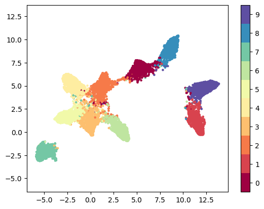
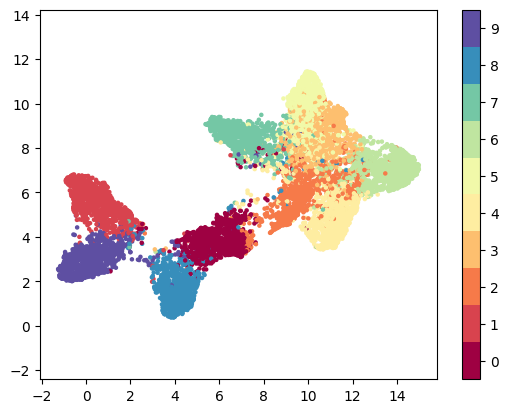
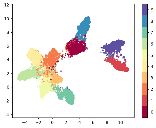
(a) Representation by supervised training without pruning (left), pruned 95% by GMP (center) and One-Shot (right).

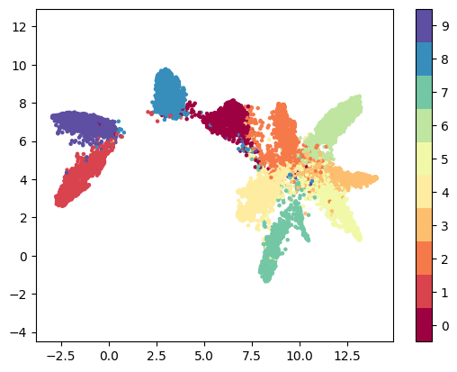
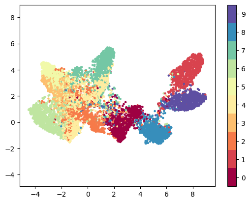
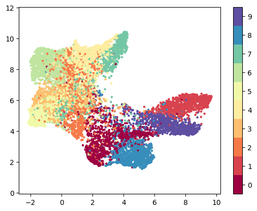
(b) Representation by supervised contrastive training without pruning (left), pruned 95% by GMP (center) and One-Shot (right).

Figure 1: Impact of pruning on the learned representation. UMAP diagrams of the models trained with supervised (top row) and supervised contrastive (bottom row) learning using WideResNet on CIFAR-10. Supervised contrastive learning is more susceptible to representation quality reduction at high sparsity than supervised learning.

This paper studies the impact of different versions of magnitude pruning on the representation learned by deep models trained with a supervised cross-entropy loss (Sup) and supervised contrastive learning (SCL) (Khosla et al., 2020) methods. We investigate the impact of changing the pruning schedule, comparing the impact of post-training global one-shot pruning (One-Shot) (Paganini & Forde, 2020), Gradual Magnitude Pruning (GMP) (Zhu & Gupta, 2017) and a delayed version of GMP ($\Delta$GMP) on the learned representation. Along with the obtained test set accuracy and the analysis of Pruning Identified Exemplars (PIEs) (Hooker et al., 2019), we also evaluate the Q-Score (Kalibhat et al., 2022), prediction depth PD-Score (Baldock et al., 2021) metrics and visually inspect obtained representations with UMAP (McInnes et al., 2018b) to draw our conclusions.

This work makes the following contributions:

• We show that models trained with SCL are significantly more impacted by all considered sparsification methods than the models trained with supervised learning trained to the same levels of sparsity. The negative impact is the highest early-on in training.

• We found that with higher sparsity representations learned by SCL decline more in quality than for supervised learning. This motivates the need for pruning methods that are more friendly to SCL models.

The next section details our experimental setup and the measures we use to assess representation quality. To quantify the amount of examples lost due to pruning, we use the evaluation framework introduced by Hooker et al. (2019) and find Pruning Identified Exemplars (PIEs) that are systematically more impacted by the introduction of sparsity. We then compare the values of several representation quality measures found in the literature to support our hypothesis that contrastive methods suffer more from sparsification than supervised training, in particular in the early phases of training.

Spar-	Sup / GMP		Sup / One-Shot		SCL / GMP		SCL / $\Delta$GMP		SCL / One-Shot
sity	(Ours)
%	PIE⋆	Acc[%]	PIE	Acc[%]	PIE	Acc[%]	PIE	Acc[%]	PIE	Acc[%]
0	-	90.58$\pm 0.38$	-	90.58$\pm 0.38$	-	92.06 $\pm 0.17$	-	92.06 $\pm 0.17$	-	92.06$\pm 0.17$
30	188	90.5$\pm 0.39$	90	90.3$\pm 0.39$	180	91.58$\pm 0.2$	176	91.59$\pm 0.18$	233	93.28$\pm 0.17$
50	179	90.4$\pm 0.34$	95	90.37$\pm 0.37$	241	90.92$\pm 0.18$	184	91.23$\pm 0.16$	236	93.06$\pm 0.2$
70	204	90.14$\pm 0.34$	97	90.33$\pm 0.37$	350	89.58$\pm 0.2$	271	90.48$\pm 0.25$	235	92.38$\pm 0.17$
90	273	89.47$\pm 0.36$	183	89.64$\pm 0.34$	748	85.56$\pm 0.4$	522⋄	87.76$\pm 0.33^{\diamond}$	549	87.83$\pm 0.25$

Table 1: Comparison of the number of PIEs for different training and pruning methods. SCL models show a more pronounced drop in performance (higher number of PIEs, lower accuracy) with higher sparsity compared to Sup models. Pruning later in training (One-Shot pruning and $\Delta$GMP) is more friendly to representation learning than early sparsification in training (GMP). ^⋆Our results differ from those reported in (Hooker et al., 2019) due to a different model architecture. ^⋄Results are aggregated over 25 models instead of 30.

2 Training, Sparsification and Measures

Training methods.

We use a WideResNet (Zagoruyko & Komodakis, 2016) architecture trained on CIFAR-10 (Krizhevsky et al., 2009) throughout our experiments for SCL and Sup training. The encoder part of the network contains 690k parameters and it is followed by a classification head realizing part of the supervised task. For SCL training our setup follows the structure proposed in (Chen et al., 2020). The encoder is first trained with a contrastive loss on an augmented version of the dataset by using a projection head discarded at the end of training, then the classification head is fine-tuned with supervised training. We use the code from the official repository (Hob, ) and follow the parameter settings used in (Hooker et al., 2019) and summarized in Appendix A. Pytorch code to reproduce the experiment is released at anonymous.4open.science/What-Is-Lost.

Pruning methods and schedules.

We implement different versions of magnitude pruning to compare the relative merits and impact of different techniques. Global post-training one-shot pruning (One-Shot) (Paganini & Forde, 2020) is the simplest method operating on a fully learned representation. We use fine-tuning to recover accuracy loss due to One-Shot pruning. Fine-tuning is performed using a Supervised loss function. Gradual Magnitude Pruning (GMP) (Zhu & Gupta, 2017) is also used in (Hooker et al., 2019) to investigate how pruning impacts different classes. A delayed version of GMP ($\Delta$GMP) starting from epoch 50 is evaluated for contrastive models. The $\Delta$GMP pruning is used to compare earlier pruning against later pruning in terms of the impact on the quality of the compressed representation.

PIEs.

We evaluate all methods based on their generalization performance, i.e., test-set accuracy. To quantify the impact of compression on the model performance, we assess the level of disagreement between the predictions of compressed and non-compressed networks on a given example. As defined in (Hooker et al., 2019), for each sample image $i$ and a set of trained models M, we denote the class predicted most frequently by the $t$-pruned models by $y_{i,t}^{M}$ and the class predicted most frequently by uncompressed models ($t=0$) by $y_{i,0}^{M}$. The sample $i$ is classified as a Pruning Identified Exemplar (PIE) iff the label is different between the set of $t$-pruned models and the set of dense models.

$$\textrm{PIE}_{i,t}=\begin{cases}1&\textrm{if }y_{i,0}^{M}\neq y_{i,t}^{M}\\ 0&\textrm{otherwise}.\end{cases}$$ (1)

As reported in (Hooker et al., 2019) pruning introduces selective forgetting, i.e., the impact of sparsity is not equally distributed amongst classes. Instead, some classes are more impacted than others. This unbalanced forgetting phenomena is stronger with lower sparsity and tends to be amplified as sparsity increases. The PIEs framework helps to quantify the impact of sparsity on the classes affected by pruning by detecting the examples for which the average prediction changes due to model pruning compared to the uncompressed version of the same model.

Batch size $N$, trained encoder $f(\cdot)$, test set $D$; Load $D$with batch size $N$. Representation vector $h_{i}$is flattened to obtain features vector of the last convolutional layer of the encoder network $f(s_{i})$. {Q-Score, Z-Score and $\|h_{i}\|_{1}$}. minibatch $\{x_{i}\}_{i=1}^{N}$i $\in\{1,\dots,N\}$$h_{i}\leftarrow f(s_{i})\in\mathbb{R}^{l}$$h_{i}\leftarrow\frac{h_{i}}{\|h_{i}\|_{2}}$Perform L2 normalization $\text{Q}_{i}\leftarrow\frac{\text{Z-Score}(h_{i})}{\|h_{i}\|_{1}}$Compute Q-Score Store $\|h_{i}\|_{1}$, Z-Score and Q-Score for analysis

Algorithm 1 Q-Score computation procedure

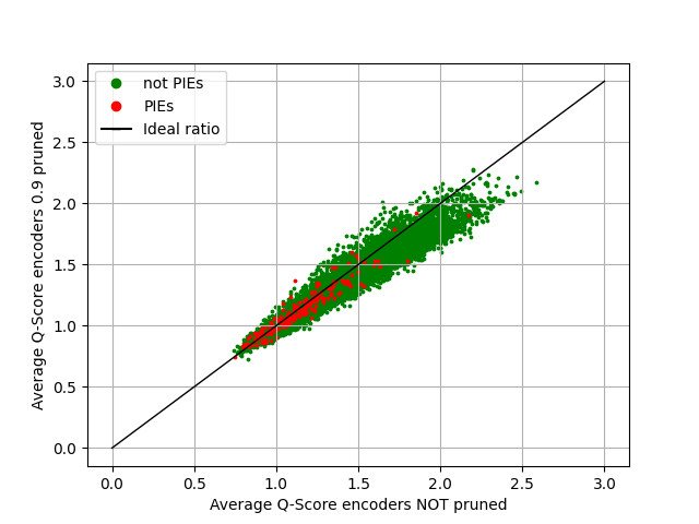
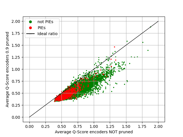
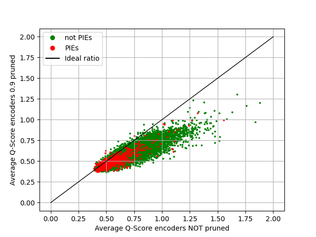
Figure 2: Q-Score analysis of the impact of pruning on the quality of learned representation. In all plots Q-Score of a non-pruned network (x-axis) is compared to the Q-Score of a pruned network with 90% sparsity (y-axis). Left to right: Sup / GMP, Sup / One-Shot, SCL / GMP, SCL / One-Shot. Q-Score of SCL models degrades at high sparsity while for Sup models it remains stable. See Appendix Section C, Table 4 and Table 5 for the Q-Score values for other sparsity levels.

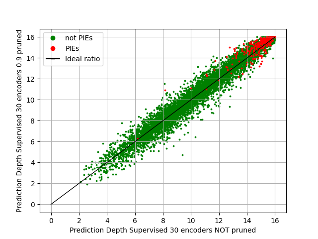
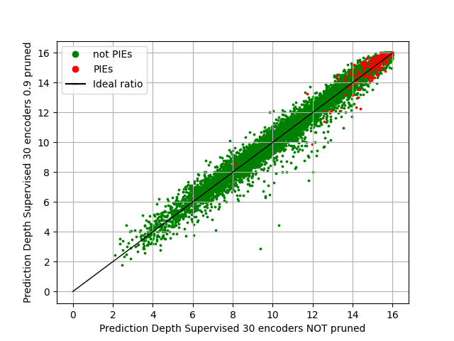
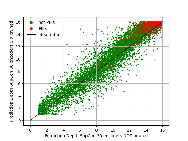
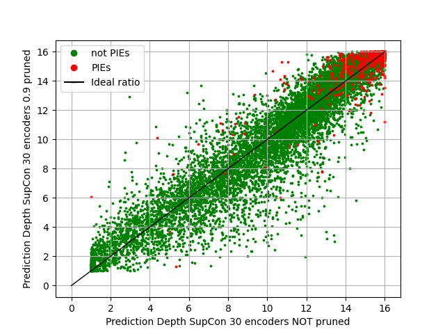
Figure 3: PD-Score analysis of the impact of pruning on the quality of learned representations. In all plots PD-Score of a non-pruned network (x-axis) is compared to the PD-Score of a pruned network with 90% sparsity (y-axis). Left to right: Sup / GMP, Sup / One-Shot, SCL / GMP, SCL / One-Shot. For Sup models, PD-Score of a sample in uncompressed model is a good predictor of PD-Score of a pruned model (points lie close to the identity line). For SCL PD-Score of a sample may change drastically due to pruning, thus high variance in two SCL plots for both GMP and One-Shot pruning on the right. See Appendix Section C for further analysis.

Q-Score.

Recently introduced by Kalibhat et al. (2022), Q-Score is an unsupervised metric to quantify the quality of the latent representation of a sample produced by an encoder network. It can be used as a regularizer during training to let the network produce a better latent representation. As shown in (Kalibhat et al., 2022), learned representations of correctly classified samples (1) have few discriminative features, i.e., higher feature sparsity, and (2) the feature values deviate significantly from the values of other features. These two properties are encoded in Q-Score defined as follows:

$$\text{Q}_{i}=\frac{\text{Z-Score}(h_{i})}{\|h_{i}\|_{1}},$$ (2)

where $h_{i}$ is a latent representation of a sample $i$, $\|h_{i}\|_{1}$ is its L1 norm and Z-Score is computed as $\frac{\mathrm{max}(h_{i}-\mu_{i})}{\sigma_{i}}$. A sample with a high Q-Score has high probability to be classified correctly (Kalibhat et al., 2022).

Prediction depth (PD-Score).

PD-Score introduced in (Baldock et al., 2021) is a supervised metric which measures sample difficulty based on the depth of a network required to correctly represent the sample. It uses an encoder network where, for each representation, a $k$-Nearest Neighbors (kNN) (Fix & Hodges Jr, 1952; Cover & Hart, 1967) classifier is trained using hidden representations of each sample in the training set. The prediction depth score of a sample is determined by the depth from which its hidden representation is correctly classified for all the subsequent kNNs. (Baldock et al., 2021) show that difficult samples, i.e., samples that are easily misclassified, have high prediction depth.

UMAP.

In this work we also illustrate the UMAP of the representation vectors after applying different pruning methods. UMAP (McInnes et al., 2018a) is a dimensionality reduction algorithm created over a mathematical framework which preserves pairwise and global distance structures of the data projected onto a lower dimensional space. Compared to other dimensionality reduction algorithms, UMAP has no restrictions on the size of the embedding vectors.

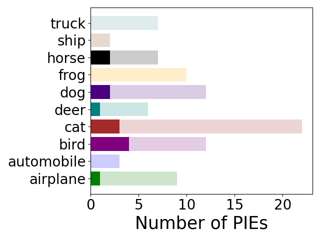
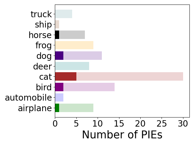
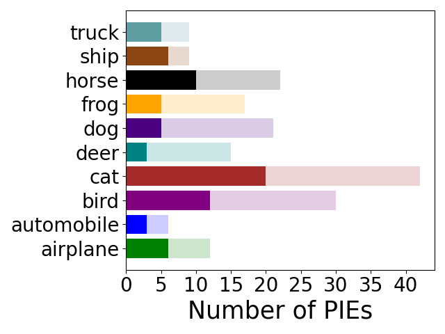
(a) PIEs obtained by One-Shot pruning Sup models: 30% (left), 50% (center) and 90% (right) sparsity.

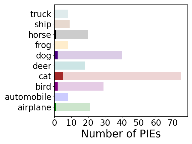
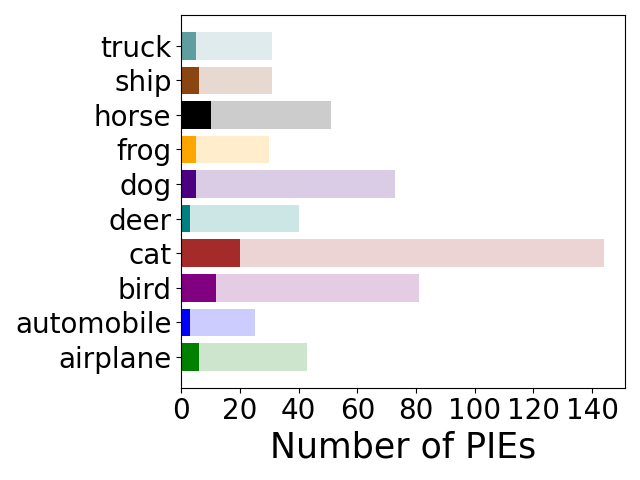
(b) PIEs obtained by One-Shot pruning SCL models: 30% (left), 50% (center) and 90% (right) sparsity.

Figure 4: Impact of pruning on PIE distribution with 30 models. Strong colors represent the number of PIEs shared between Sup and SCL models; light colors represent unique PIEs.

3 Evaluation

Following (Hooker et al., 2019), 30 WideResNet16-2 models were trained with SGD on CIFAR10 for each sparsity and learning method. The length of the representation vector $l$ is chosen equal to 128. We prune the networks to achieve sparsity levels $t\in\{0,30,50,70,90\}$%. GMP (Zhu & Gupta, 2017) and $\Delta$GMP prune models during training, whereas One-Shot applies pruning post-training followed by finetuning. Below we compare the results obtained for Sup and SCL models with respect to the distribution of PIEs and compare the representation obtained by pruned models to the one learned by uncompressed models.

3.1 Impact of Sparsity on Distribution of PIEs

The model test-set accuracy and the total number of counted PIEs are summarized in Table 1. The comparison between GMP and One-Shot pruning for Sup models shows that the latter yields the lower number of PIEs across all pruning ratios. Among SCL models, the lowest number of PIEs is achieved by $\Delta$GMP across all sparsity levels (except for 70% of sparsity). We also observe that SCL models forget more easily than Sup models for sparsities over 30%.

The performance sensitivity with respect to individual classes is amplified as sparsity increases. In Figure 4 we observe a similar behavior in our experiments as reported in (Hooker et al., 2019): The number of samples being lost by Sup and SCL models gets more uniformly distributed across classes with higher sparsity. This uniform loss phenomenon is best observed when 95% and 99% compression is applied to the models, also shown in Appendix Figure 7.

3.2 Impact of Sparsity on Representation Quality

We compute Q-Score for each sample by taking an average of 30 pruned and non-pruned models. Q-Score decreases with higher sparsity and this trend is considerably more pronounced in SCL than in Sup models for both GMP and One-Shot pruning algorithms, as shown in Figure 2 for 90% sparsity. The average Q-Score obtained for SCL and Sup models for other sparsity levels is reported in Table 4 and Table 5 in the appendix. Even though we observe higher Q-Score for Sup than for SCL learning, we believe it is incorrect to compare Q-Score across learning methods due to differences in the loss function and different implicit bias. Note that high variance in Q-Score, Z-Score and $||h_{i}||_{1}$ prevents a more fine-grained analysis.

PD-Score for each sample is computed by taking the average of 5 pruned or 5 non-pruned models. In Figure 3 the PD-Score of samples processed with Sup and SCL models for 90% sparsity is compared to PD-Score computed for uncompressed models. Average PD-Score for different sparsity levels is reported in Appendix Table 6. PD-Score is higher for PIEs and lower for the correctly classified samples. For Sup models, PD-Score of a sample in uncompressed model is a good predictor of PD-Score of that sample in a pruned model. For SCL, PD-Score of a sample may change drastically due to pruning, and thus we observe high variance in two SCL plots on the left for both GMP and One-Shot pruning.

A qualitative analysis of the sparsified representations based on UMAP and visualization of individual PIEs is discussed in Section D in the Appendix. We show that difficult examples are largely unique for a training and pruning combination for low sparsity values even though the distribution of PIEs over classes looks similar. This is a peculiar phenomenon that requires further investigation.

4 Discussion

This paper explores the impact of magnitude pruning on supervised contrastive learning and compares the impacted representation quality to supervised learning using several metrics described in the literature. Our findings suggest that models optimized with a contrastive objective are more sensitive to the introduction of sparsity relatively to traditional supervised training with a cross-entropy loss. Sparsity in these optimization settings significantly increases disparate error between classes at high levels of sparsity. In particular, sparsification of models trained using a contrastive objective leads to $\times$3 as many misclassified examples as supervised learning models sparsified with global post-training magnitude pruning, in the best setting. Curiously enough, difficult examples are largely unique across considered training methods for low sparsities, but the overlap grows with higher sparsity. We hope this work sparks interest in developing more representation-friendly pruning methods for supervised contrastive learning.

Appendix

Appendix A Training parameters

Table 2 summarizes the set of used hyper-parameters for training different networks. We refer to the corresponding papers describing the details of the SCL loss function and the data augmentation methods.

All experiments were performed on the TU Graz computing infrastructure.

Hyperparameter	Sup	SCL
Dropout	Not used
Weight decay	5e-4
Batch size	128	1024
# epochs	205	500
Loss function	Cross-entropy	(Khosla et al., 2020)
Optimizer	SGD
Learning rate	1.0	0.05
Momentum	0.9
Data Augment.	Rnd. Crop,	(Nakkiran et al., 2020)
	Horiz. Flip
Label smoothing	Not used
Sparsity begin step	1000	125
Sparsity end step	20000	2476
Pruning frequency	500	62
Cosine Annealing	Not used	Used
Warmup epochs	Not used
Temperature	Not used	0.5
Network type	WideResNet

Table 2: Training hyper-parameters.

Appendix B PIE Comparison

Sparsity	Sup  / GMP ⋆	Sup  / GMP
	Hooker et al. (2019)	(Ours)
%	PIE	PIE	Acc[%]
0	-	-	90.58 $\pm 0.38$
30	114	188	90.5 $\pm 0.39$
50	144	179	90.4 $\pm 0.34$
70	137	204	90.14 $\pm 0.34$
90	216	273	89.47 $\pm 0.36$

Table 3: Comparison of the number of PIEs for different training pruning methods. Our results differ from those reported in (Hooker et al., 2019) due to a different model architecture used.

We closely follow the setup by Hooker et al. (2019) to compute the number of PIEs for the Sup  / GMP setting. We obtain slightly different results due to the use of a different network architecture. The comparison is detailed in Table 3.

Appendix C Representation Quality Scores

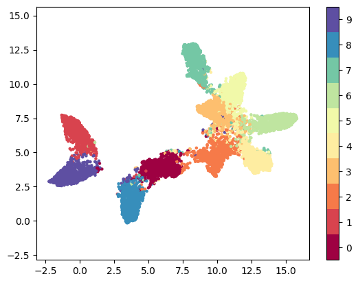
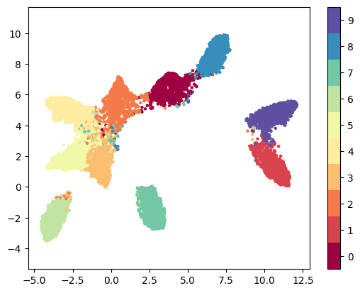
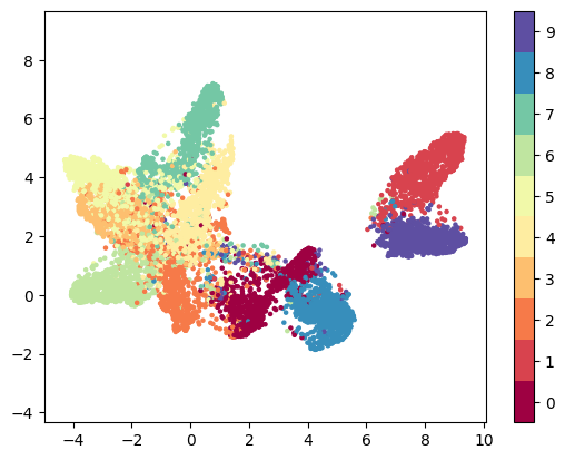
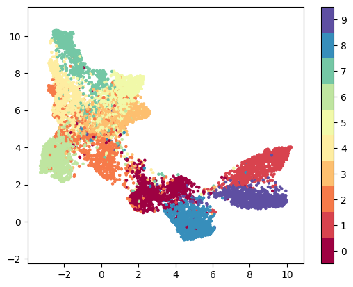
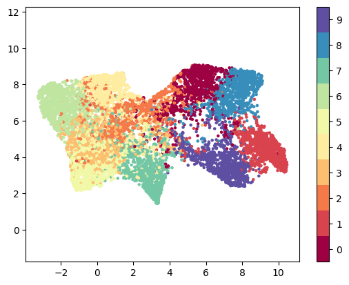
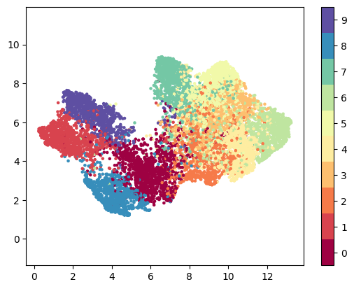
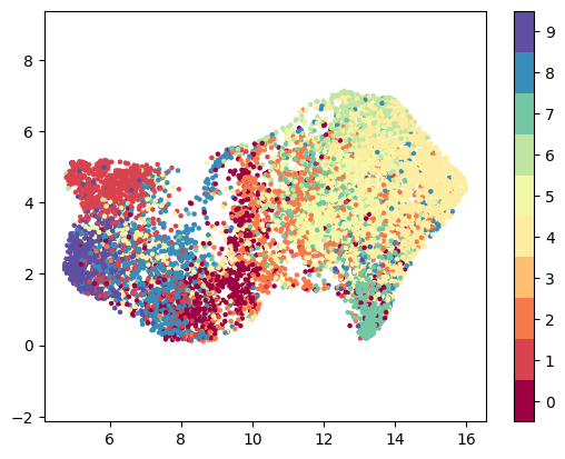
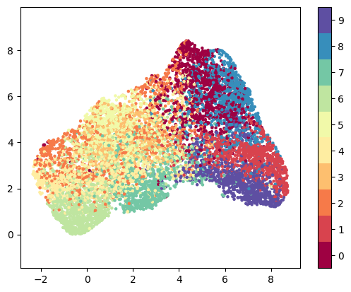
Figure 5: UMAP analysis of the impact of different pruning methods on the learned representations. The top row presents the results for Sup (left) and SCL (right) models trained with 0% sparsity. The second and the third rows present the results when applying 90% and 99% sparsity, respectively. Left to right: Sup  / GMP, Sup  / One-Shot, SCL  / GMP, SCL  / One-Shot.

A detailed comparison of UMAPs obtained for different sparsities is shown in Figure 5. We observe that representations learned by SCL degrade fast with higher sparsity resulting in a cloud of points. Although UMAP diagrams do not reflect discriminator performance, we can observe that representation projections of Sup and SCL models are fairly different.

Sparsity	SCL  / GMP			SCL  / One-Shot
%	Q	Z	$||h_{i}||_{1}$	Q	Z	$||h_{i}||_{1}$
0	0.72$\pm 0.17$	5.01$\pm 0.62$	7.15$\pm 0.8$	0.72$\pm 0.16$	5.01$\pm 0.62$	7.15$\pm 0.8$
30	0.69$\pm 0.16$	4.95$\pm 0.65$	7.34$\pm 0.81$	0.66$\pm 0.14$	4.92$\pm 0.61$	7.6$\pm 0.76$
50	0.66$\pm 0.16$	4.84$\pm 0.64$	7.5$\pm 0.82$	0.65$\pm 0.14$	4.93$\pm 0.63$	7.71$\pm 0.76$
70	0.62$\pm 0.15$	4.68$\pm 0.6$	7.74$\pm 0.82$	0.63$\pm 0.08$	4.96$\pm 0.63$	7.95$\pm 0.74$
90	0.56$\pm 0.13$	4.47$\pm 0.57$	8.14$\pm 0.82$	0.59$\pm 0.01$	4.89$\pm 0.57$	8.39$\pm 0.66$

Table 4: Representation quality assessed by Q-Score for SCL trained models. Representation quality of SCL models is affected by pruning. This can be seen by a fast degradation of the Q-Score value with higher sparsity compared to the Sup setting (see Table 5). Sparsity affects both Z-Score and $||h_{i}||_{1}$ resulting in a lower Z-Score and a higher $||h_{i}||_{1}$.

Sparsity	Sup  / GMP			Sup  / One-Shot
%	Q	Z	$||h_{i}||_{1}$	Q	Z	$||h_{i}||_{1}$
0	1.44$\pm 0.29$	5.73$\pm 0.68$	4.15$\pm 0.4$	1.44$\pm 0.29$	5.73$\pm 0.68$	4.15$\pm 0.4$
30	1.43$\pm 0.3$	5.71$\pm 0.69$	4.19$\pm 0.41$	1.41$\pm 0.28$	5.68$\pm 0.67$	4.19$\pm 0.39$
50	1.41$\pm 0.29$	5.66$\pm 0.68$	4.2$\pm 0.41$	1.42$\pm 0.29$	5.69$\pm 0.68$	4.19$\pm 0.39$
70	1.39$\pm 0.28$	5.61$\pm 0.65$	4.2$\pm 0.4$	1.42$\pm 0.26$	5.69$\pm 0.67$	4.19$\pm 0.39$
90	1.39$\pm 0.27$	5.66$\pm 0.64$	4.21$\pm 0.38$	1.38$\pm 0.26$	5.72$\pm 0.66$	4.3$\pm 0.35$

Table 5: Representation quality assessed by Q-Score for Sup trained models. Representation quality of Sup models is not affected as sparsity increases, since Z-Score and $||h_{i}||_{1}$ stay close to the values of non-pruned models (0% sparsity).

Complementing Figure 2 discussed in the main paper, Table 4 and Table 5 show the performance of GMP and One-Shot pruning methods for SCL and Sup learning respectively. Even though we observe higher values of Q-Score for Sup than for SCL learning, we believe it is not correct to compare Q-Score values across different representation learning methods, mainly due to differences in the loss function and different implicit bias. However, when comparing GMP to One-Shot pruning for Sup models, both perform fairly stable over a large range of sparsities. This is different for SCL models, where Q-Score shows a significant drop with higher sparsity.

Sparsity	Sup  / GMP		Sup  / One-Shot		SCL  / GMP		SCL  / One-Shot
%	PIE	non-PIE	PIE	non-PIE	PIE	non-PIE	PIE	non-PIE
0	14.87$\pm 0.96$	10.85$\pm 2.82$	14.87$\pm 0.96$	10.85$\pm 2.82$	14.67$\pm 1.45$	9.94$\pm 2.91$	14.67$\pm 1.45$	9.94$\pm 2.91$
30	14.87$\pm 1.01$	10.98$\pm 2.75$	14.95$\pm 1.09$	11$\pm 2.82$	14.95$\pm 1.91$	10.35$\pm 4.15$	14.67$\pm 1.86$	9.67$\pm 4.03$
50	14.89$\pm 1.1$	10.84$\pm 2.94$	14.92$\pm 1.17$	10.97$\pm 2.93$	15.09$\pm 1.64$	10.36$\pm 4.2$	14.69$\pm 1.99$	9.71$\pm 4.06$
70	15.03$\pm$ 1.2	11.01$\pm 2.86$	14.85$\pm 1.18$	10.89$\pm 2.86$	15.14$\pm 1.81$	10.44$\pm 4.23$	14.56$\pm 2.23$	9.79$\pm 4.03$
90	15.1$\pm 1.13$	11.03$\pm 2.91$	14.97$\pm 1.13$	10.89$\pm 2.91$	15.15$\pm 1.71$	10.48$\pm 4.29$	14.97$\pm 1.7$	10$\pm 4.18$

Table 6: Representation quality assessed by PD-Score for Sup and SCL trained models. PD-Score of SCL models has higher variance than for Sup models indicating that pruning is oblivious to representation quality learned by SCL.

PD-Score analysis for 90% sparsity is visualized in Figure 3. As can be observed from the plots obtained for Sup learning the PD-Score of sparse models and uncompressed models tend to be equal, points lie close to the ideal ratio line. For SCL models instead PD-Score points are more scattered, PD-Score of sparse SCL models is not similar to PD-Score obtained from uncompressed SCL models. The same effect can also be observed in Table 6: The variance of PD-Score for SCL models is higher than for Sup models. These observations confirm that SCL models’ behavior is significantly different when pruning is applied, while for Sup models this is not the case.

Appendix D PIE Distribution and Visualization

In Figure 6 we visualize a few sample images and show the corresponding predicted classes for correctly classified images by a sparse SCL model which are, however, wrongly classified by an uncompressed SCL model.

In Figure 7 the distribution of PIEs are visualized for all the pruning percentages. As sparsity increases PIEs distribution tends to be more uniform: For 95% and 99% sparsity the number of PIEs shared between Sup and SCL models is higher. This trend was also observed by (Hooker et al., 2019).

U: Ship S: Automobile

U: Ship S: Airplane

U: Cat S: Dog

U: Airplane S: Cat

U: Cat S: Deer

U: Truck S: Automobile

U: Ship S: Deer

U: Airplane S: Automobile

U: Deer S: Horse

U: Deer S: Ship

U: Airplane S: Deer

U: Dog S: Cat

Figure 6: Correctly classified samples by SCL 30% sparse model and missclassified by SCL dense model. The eight images on top (first two rows) are correctly classified by GMP pruned model while the four images on bottom are correctly classified by One-Shot pruned model. For each image, the class prediction from the uncompressed model (U) is shown on the left while for the sparse model (S) on the right.

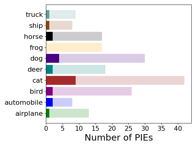
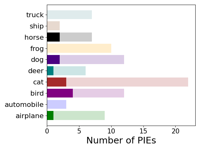
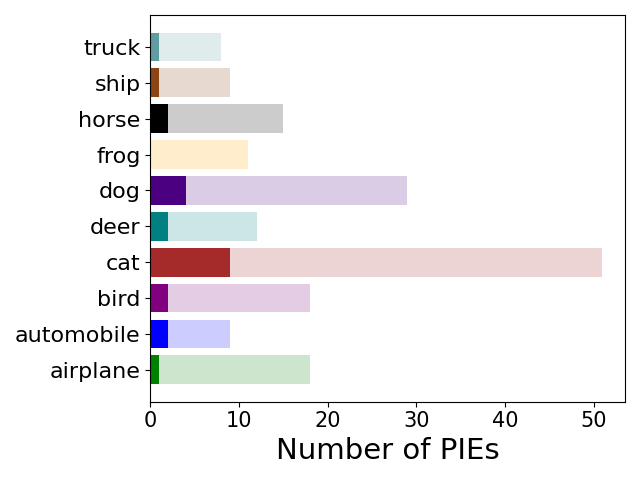
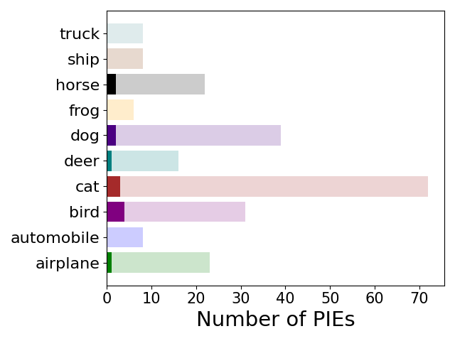
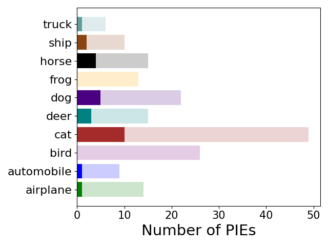
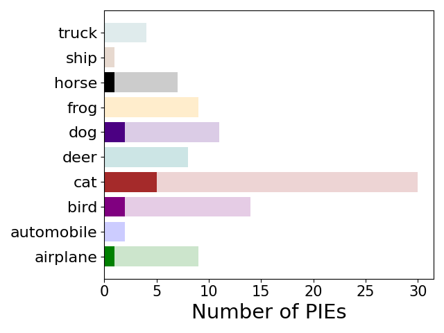
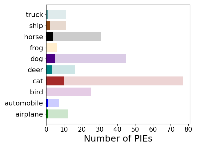
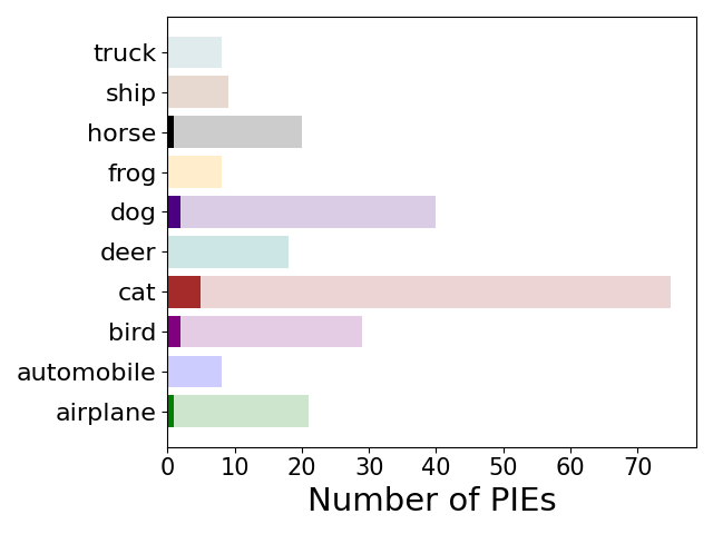
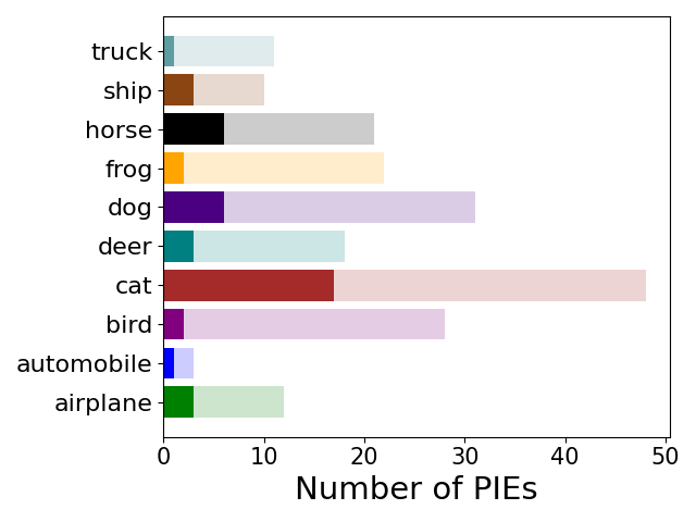
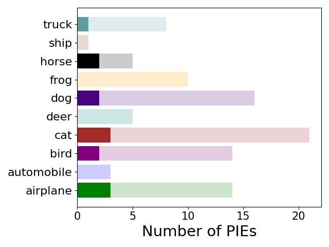
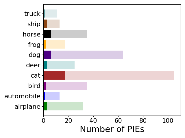
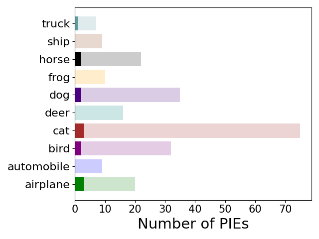
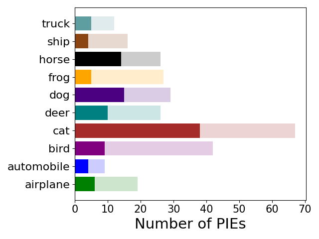
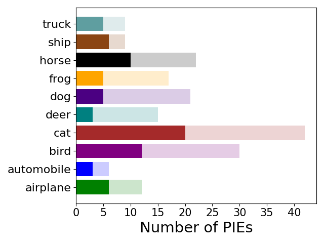
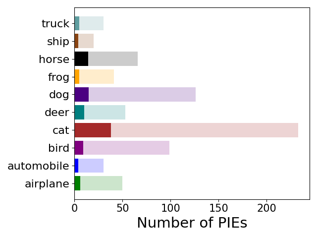
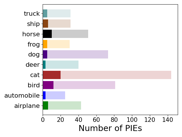
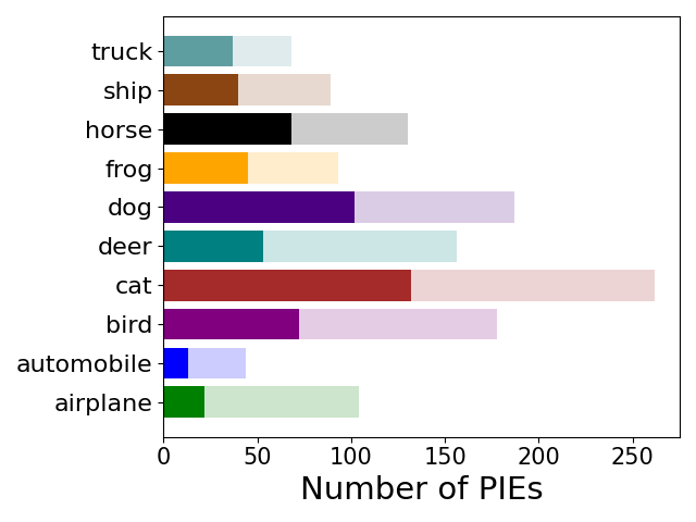
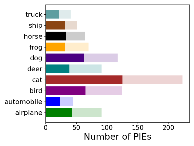
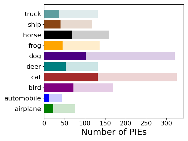
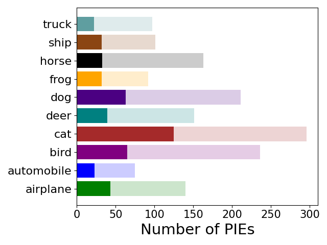
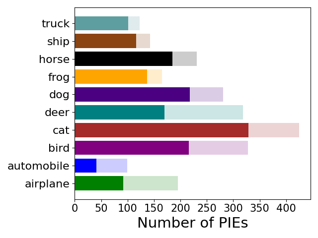
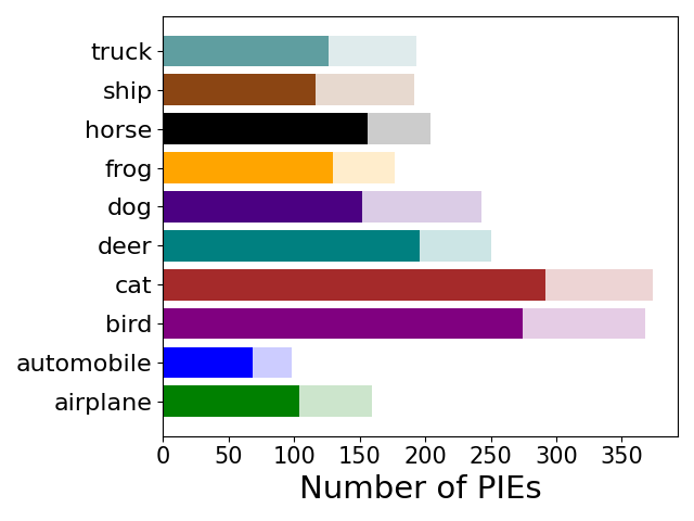
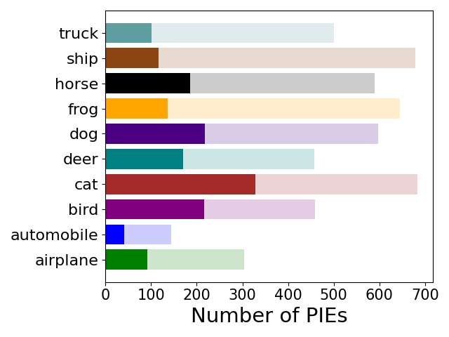
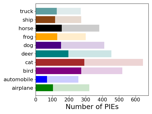
Figure 7: PIE distribution over classes for different sparsity levels. From top to bottom: 30%, 50%, 70%, 90%, 95% and 99% sparsity. In each column from left to right: Sup / GMP, Sup / One-Shot, SCL / GMP, SCL / One-Shot. Color bars depict the number of PIEs identified in each class. Strong colors show the number of PIEs that are the same for Sup and SCL models and can be considered as difficult examples regardless of the training method. Light colors show the number of unique PIEs for a training method. Curiously, the number of PIEs that are universal for both training methods is low for low sparsities, even though the distribution of PIEs over classes looks similar.

References

- (1) Supervised contrastive repository. https://github.com/HobbitLong/SupContrast.
- Baldock et al. (2021) Baldock, R., Maennel, H., and Neyshabur, B. Deep learning through the lens of example difficulty. Advances in Neural Information Processing Systems, 34, 2021.
- Chen et al. (2020) Chen, T., Kornblith, S., Norouzi, M., and Hinton, G. A simple framework for contrastive learning of visual representations. pp. 1597–1607, 2020.
- Cover & Hart (1967) Cover, T. and Hart, P. Nearest neighbor pattern classification. IEEE transactions on information theory, 13(1):21–27, 1967.
- Entezari & Saukh (2019) Entezari, R. and Saukh, O. Class-dependent compression of deep neural networks. arXiv preprint arXiv:1909.10364, 2019.
- Fix & Hodges Jr (1952) Fix, E. and Hodges Jr, J. L. Discriminatory analysis-nonparametric discrimination: Small sample performance. Technical report, California Univ Berkeley, 1952.
- Han et al. (2015a) Han, S., Mao, H., and Dally, W. J. Deep compression: Compressing deep neural networks with pruning, trained quantization and huffman coding. arXiv preprint arXiv:1510.00149, 2015a.
- Han et al. (2015b) Han, S., Pool, J., Tran, J., and Dally, W. Learning both weights and connections for efficient neural network. Advances in neural information processing systems, 28, 2015b.
- Hooker et al. (2019) Hooker, S., Courville, A., Clark, G., Dauphin, Y., and Frome, A. What do compressed deep neural networks forget? arXiv preprint arXiv:1911.05248, 2019.
- Kalibhat et al. (2022) Kalibhat, N. M., Narang, K., Tan, L., Firooz, H., Sanjabi, M., and Feizi, S. Understanding failure modes of self-supervised learning. arXiv preprint arXiv:2203.01881, 2022.
- Khosla et al. (2020) Khosla, P., Teterwak, P., Wang, C., Sarna, A., Tian, Y., Isola, P., Maschinot, A., Liu, C., and Krishnan, D. Supervised contrastive learning. Advances in Neural Information Processing Systems, 33:18661–18673, 2020. URL https://arxiv.org/abs/2004.11362.
- Krizhevsky et al. (2009) Krizhevsky, A., Nair, V., and Hinton, G. Cifar-100 and cifar-10 (canadian institute for advanced research), 2009. URL http://www.cs.toronto.edu/~kriz/cifar.html. MIT License.
- McInnes et al. (2018a) McInnes, L., Healy, J., and Melville, J. Umap: Uniform manifold approximation and projection for dimension reduction. arXiv preprint arXiv:1802.03426, 2018a.
- McInnes et al. (2018b) McInnes, L., Healy, J., Saul, N., and Großberger, L. Umap: Uniform manifold approximation and projection. Journal of Open Source Software, 3(29):861, 2018b. doi: 10.21105/joss.00861. URL https://doi.org/10.21105/joss.00861.
- Nakkiran et al. (2020) Nakkiran, P., Neyshabur, B., and Sedghi, H. The deep bootstrap framework: Good online learners are good offline generalizers, 2020. URL https://arxiv.org/abs/2010.08127.
- Paganini & Forde (2020) Paganini, M. and Forde, J. Streamlining tensor and network pruning in pytorch. arXiv preprint arXiv:2004.13770, 2020.
- Timpl et al. (2021) Timpl, L., Entezari, R., Sedghi, H., Neyshabur, B., and Saukh, O. Understanding the effect of sparsity on neural networks robustness. In ICML 2021 Workshop Overparameterization: Pitfalls & Opportunities. ICML workshop, 2021.
- Zagoruyko & Komodakis (2016) Zagoruyko, S. and Komodakis, N. Wide residual networks. arXiv preprint arXiv:1605.07146, 2016.
- Zhu & Gupta (2017) Zhu, M. and Gupta, S. To prune, or not to prune: exploring the efficacy of pruning for model compression. arXiv preprint arXiv:1710.01878, 2017.