Comprehensive Reactive Safety:
No Need For A Trajectory If You Have A Strategy

Abstract

Safety guarantees in motion planning for autonomous driving typically involve certifying the trajectory to be collision-free under any motion of the uncontrollable participants in the environment, such as the human-driven vehicles on the road. As a result they usually employ a conservative bound on the behavior of such participants, such as reachability analysis. We point out that planning trajectories to rigorously avoid the entirety of the reachable regions is unnecessary and too restrictive, because observing the environment in the future will allow us to prune away most of them; disregarding this ability to react to future updates could prohibit solutions to scenarios that are easily navigated by human drivers. We propose to account for the autonomous vehicle’s reactions to future environment changes by a novel safety framework, Comprehensive Reactive Safety. Validated in simulations in several urban driving scenarios such as unprotected left turns and lane merging, the resulting planning algorithm called Reactive ILQR demonstrates strong negotiation capabilities and better safety at the same time.

I INTRODUCTION

Safety is of central concern in the development of autonomous driving systems, frequently cited as one of the areas where AI drivers could bring significant improvement over their human counterparts [1, 2]. Indeed, equipped with vastly superior computational power in solving differential equations and geometric intersections while never making random mistakes or losing focus, AI vehicle operators are expected to outperform humans in their ability to foresee and prevent collisions. This outlook motivated a large body of work employing tools such as reachability analysis ([3, 4, 5]) to plan or certify safe trajectories, on the principle that a trajectory is safe if and only if it can be proven to be disjoint from any region in space-time that could potentially be occupied by any (dynamic or static) obstacle. While theoretically appealing, these approaches prove inadequate when deployed in practical autonomous driving solutions.

One of the major difficulties facing these reachability-based approaches is that they can be so conservative that it becomes impossible for the autonomous vehicle to make any progress. Figure 1 shows a common scenario where the autonomous vehicle (abbreviated AV below) is trying to drive past a slow moving vehicle in an adjacent lane. Due to their potential intention of lane change that is unknowable to the AV, the reachable set of the slow vehicle will quickly fill up both lanes in a few seconds, which is not enough time for the AV to complete the overtake. The range of potential acceleration on the slow vehicle also allows it to appear in a wide range of longitudinal positions at any moment, therefore the vehicle’s reachable set essentially covers the entire space-time region in front of the AV. As a result, in order to avoid any intersection with the reachable set, the AV has to brake and trail behind the slow vehicle’s longitudinal position, as if following it as a lead vehicle, despite the fact that it is in a different lane.

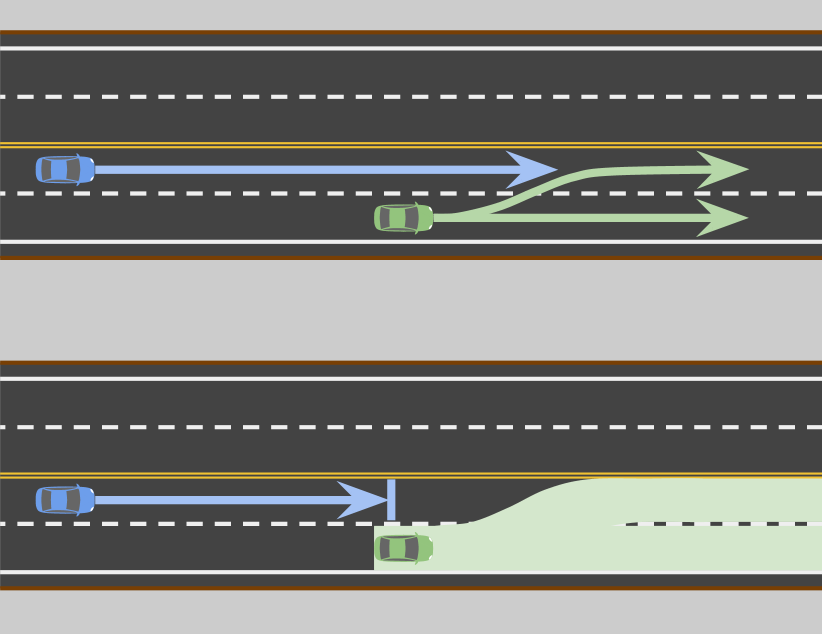
Figure 1: A scenario where the fast autonomous vehicle (blue) is overtaking a slow vehicle (green). The potential lane keeping and lane change trajectories of the other vehicle are drawn as green arrows on the top; the corresponding (spatial) reachable sets are drawn on the bottom. The unbounded growth of the reachable set eventually blocks all the ways to make progress.

The way current safety techniques utilize the reachability analysis is conservative by nature. Having the trajectory being disjoint from the reachable set is well sufficient for proving the absence of any possibility of collision, but it is far from necessary. The reachable set of a dynamic object generally grows unboundedly over time, and given enough planning horizon it will inevitably intersect with any motion of the AV that makes forward progress. On the other hand, a human driver readily knows that the slow moving vehicle is physically incapable of fully blocking both lanes: no matter which lane it decides to occupy, the other lane will be left open, and safe overtake is possible. This conclusion is obvious to human drivers, yet it is unrealized in the autonomous driving safety frameworks available today. Why?

The key insight here is that in normal driving, the trajectory produced by the planner is almost never fully executed as is. Modern urban autonomous driving systems typically run at a frequency around 10Hz, and trajectories (usually with a horizon of 10 seconds or more) are planned and executed in a pipeline, so only the initial 100 millisecond portion (about one percent) of each trajectory is actually executed by the controller before it receives and switches to execute a new trajectory. The new trajectory responds to changes in the environment by incorporating up-to-date sensor data, and thus will in general be slightly different unless the motion prediction used in the old trajectory is perfectly deterministic and accurate. Since by the time the AV gets to the latter portion of the trajectory, it would have learned more about its surroundings and found smarter things to do, why be alarmed when the limited knowledge that the AV possesses now cannot assert safety at that distant time in the future? This latter portion of the trajectory will not be executed by the vehicle, so rigorously checking for collisions on this portion of the trajectory does not benefit the overall safety of the autonomous driving system. This means that, ensuring the entire trajectory is free of collision with any potential motion of any obstacle, which is the paradigm adopted universally by all autonomous driving safety frameworks known to us, should be reconsidered. What we need is a new safety framework that takes into account how the trajectory will change in reaction to environment changes in the future, and ensures that the reaction, instead of the current trajectory, is safe.

To this end, we propose the concept of Comprehensive Reactive Safety (CRS), a condition certifying that the autonomous driving system has the ability to stay out of collision by reacting to new observations over the planning horizon, without necessarily requiring it to have a collision-free trajectory set in stone. This allows the system to respond to different future scenarios with different tailored actions, as long as it can be shown that it will have time to observe and distinguish which scenario is coming to realization before committing to an action. This freedom is crucial when a single sequence of actions safely navigating all possible future scenarios does not exist, and thus no trajectory will pass the traditional trajectory-based safety criterion. In other words, under CRS, the autonomous driving system is planning strategies, which describe what to do in response to each possible future situation, rather than planning trajectories, which describe what to do, period.

To summarize, our main contributions are:

1. We propose the Comprehensive Reactive Safety, a novel safety framework that, for the first time, accounts for how the AV reacts to future changes in the environment. This framework drastically increases the flexibility of planning and opens up possibilities for new solutions to scenarios that are challenging to traditional reachability analysis. We give proof that the much less restrictive CRS condition still guarantees safe operation of the vehicle.

2. We present the Reactive ILQR algorithm, a practical planning algorithm that satisfies CRS. With side-by-side comparisons in four representative classes of scenarios commonly found in urban driving, we demonstrate that the proposed RILQR planner is more effective in negotiating solutions when interacting with other vehicles, and capable of resolving interactions in ways not possible with the traditional reachability-based planners, all while improving safety.

The rest of the paper is organized as follows. Section II reviews reachability analysis and AV safety approaches. Then, Section III-A defines CRS and proves its validity in certifying safe driving, and Section III-B outlines the RILQR algorithm, which is evaluated in Section IV in common scenarios found on urban public roads.

II RELATED WORK

II-A Safety enforcement

Safety is typically defined as the condition and certification that no collisions exist between the trajectories of the AV and the obstacles, potentially accounting for uncertainty in both. Planners ensure the safety of the trajectories they produce by one of two categories of approaches: either construct the trajectories with safety as a constraint through search algorithms [7, 8] and constrained optimization algorithms [9, 10], or apply safety verification on the trajectories constructed with more relaxed collision constraints, and, upon finding a collision, fall back to the last verified trajectory [3], override with a fail-safe trajectory [4], or perform corrective modifications to restore safety [11].

Constrained optimization techniques are well studied in the numerical optimization literature [12, 13]. Motion planning algorithms for autonomous driving have been developed using various optimization techniques such as sequential quadratic programming (SQP) [10], linear programming (LP) [9], and mixed integer quadratic programming (MIQP) [14]. Constrained ILQR [15, 16], an extension of the Iterative Linear Quadratic Regulators (ILQR) [17, 18] to support arbitrary state constraints using barrier functions, can be used to enforce safety constraints as well. We build our implementation on top of Constrained ILQR.

II-B Sources of uncertainty

Autonomous driving systems operating in the real world are faced with a number of sources of uncertainty potentially relevant to safety, and they have been the subject of many studies. Control noise and environment disturbance can be bounded by feedback control, resulting in the expansion of the AV trajectory into an invariant set that the controller can guarantee never leaving [19]. Measurement (in positioning and perception) noise are usually treated by padding the safety constraints with buffers. Uncertainty in the AV’s knowledge about the environment due to sensor limitations, such as occlusion, can be addressed by hallucinating obstacles in occluded regions [20]. For dynamic obstacles such as vehicles, their unknown future motions and intentions are a significant source of uncertainty, for which there are conservative estimation techniques using reachability analysis [3, 11, 4], as well as a blooming body of research on data-driven motion prediction techniques [21, 22, 23] . In particular, Li et al [5] seek to mitigate the conservativeness of reachability analysis by classifying the object behavior into one of the clusters learned offline, each of which then has a more limited reachability. Our work shares their premise, but do not rely on data-driven procedures that generally lose safety guarantees, and only rule out portions of reachable sets by evidence from observed object motion.

II-C Reachability

Reachability analysis is a tool for studying dynamical systems. Some techniques formulate the process as a differential game and solve its Hamilton-Jacobi PDE [24], while others use conservative linearization to inclusively approximate the nonlinear dynamics [3]. In autonomous driving applications, reachability analysis is used to compute a conservative superset of spatial locations an object could reach as a result of its unknown intentions and actions, under certain kinematic, dynamic or behavioral assumptions.

Behavioral assumptions on the objects are adopted to curb the growth of reachable sets, usually by formalizing traffic laws [4, 6, 25]; planners avoiding the resulting smaller reachable sets cannot guarantee to not collide, but can guarantee to not be at fault in a collision. While it may help to prevent the reachable set from blocking the AV in some cases, the state of the art in this research direction has generally been limited to simple rule sets around the driving direction constraint and the safe distance, struggling to handle the complexity in real world traffic. The interpretation and formalization of human traffic rules is a much more difficult task than it might first appear [6]. Another way to keep the reachable sets manageable is to limit the planning horizon as done by Pan et al [26], who echo our observation about the unrealistic spread of reachability in the long term. However, relying on tuning the horizon to keep reachability under control makes the planner brittle, and the lack of convergence to the desired behavior as the horizon tends to infinity is theoretically unsatisfactory. Our proposed safety framework is not a replacement of reachability analysis, but rather a more flexible way of applying it, aimed at addressing its weakness of conservativeness. It can be used with any existing technique to compute reachable sets.

It is worth pointing out that, although planning around all reachable sets is unnecessarily conservative because new observations in the future will enable more targeted responses, this is not true in the worst case scenario where the autonomous driving system suffers from severe faults and loses its sensing capabilities after making a plan, which, although rare, is a risk that cannot be ignored. In such a case, execution of a plan that requires observation updates will not be possible, and safety can only be achieved by an open-loop trajectory that circumvents all currently known reachable sets. This may very well be infeasible, again because of how large the reachable sets could be, but that is just the harsh reality of trying to stay safe in this extremely challenging “glimpse-and-then-go-blind” situation. When designing a safe autonomous driving system, fallback mechanisms must be included to make the AV “limp” to a minimum safe state in hazardous situations like this, possibly involving reachability analysis. However, the necessity of evil in the worst case is no excuse for not holding ourselves to higher standards in the average cases, and with our proposed CRS framework, we do.

III METHOD

III-A Comprehensive Reactive Safety

Consider a given moment in time where the autonomous driving system is supposed to make a driving plan based on the latest perception and prediction. Without loss of generality, we call this moment $t=0$. Let $T$ denote the planning time domain $[0,t_{end}]$ and $X$ the spatial domain (usually the 2D space on the ground). A trajectory (for the AV or the objects) is a function $\tau:T\to X$, and the set of all trajectories is denoted by $\mathcal{T}=\{\tau|\tau:T\to X\}$. Given a trajectory $\tau$, we use $C_{\tau}$ to represent the corresponding swept-volume trajectory $C_{\tau}:T\to\mathcal{P}(X)$ such that $C_{\tau}(t)$ is the collision volume of the AV or the object at time $t$.

Given the set of objects $O$ reported by the perception subsystem, the prediction subsystem predicts the potential range of motion for each object $i\in O$ as a set of possible trajectories $P_{i}\subseteq\mathcal{T}$. This set can also be seen as the spatial-temporal reachable set of the object. In addition, an interaction-aware predictor would be able to give the possible combinations of individual object motions (taking into account interaction constraints such as, when two objects approach an intersection from different directions, one of them has to yield), which we call futures $F=\{(p_{1},p_{2},...,p_{N})|p_{i}\in P_{i}\}\subseteq P_{1}\times P_{2}\times...\times P_{N}$, a description of all the possible ways the future could unfold. We use the subscript notation to reference the trajectory of a particular object in a future: for $f\in F$, $f_{i}\in P_{i}$ is the trajectory of object $i$ that will be realized in this future.

The planning subsystem is responsible for producing a driving plan for the AV to follow. The traditional planner produces a trajectory $\tau\in\mathcal{T}$, and the traditional safety criterion is that it has no collision with any prediction: $C_{\tau}(t)\cap C_{p}(t)=\emptyset,\forall p\in P_{i},\forall i\in O,\forall t\in T$. This condition can be equivalently written in terms of the futures: $C_{\tau}(t)\cap C_{f_{i}}(t)=\emptyset,\forall i\in O,\forall f\in F,\forall t\in T$. On the other hand, in the spirit of ensuring safety by being able to react to anything that could happen in the future, we propose that the planner should instead produce a strategy which maps potential future situation realizations to trajectories, $\sigma:F\rightarrow\mathcal{T}$. In other words, the planner plans a trajectory for each future scenario.

To ensure the strategy can be followed by the AV (without requiring it to possess supernatural prophetic powers), it must satisfy certain causality constraints: the trajectory must “react” to the future variation after it has occurred. For example, an evasive lane change trajectory to circumvent an object cutting in must not begin the lane change before the object shows signs that it is about to cut in.

Definition 1 (Requirement I: Reaction Causality)

A strategy $\sigma$ satisfies the Reaction Causality Requirement if for any two futures $f,g\in F$ and any time $t\in T$, the condition $\sigma(f)(t)=\sigma(g)(t)$ holds as long as we have $f_{i}(t^{\prime})=g_{i}(t^{\prime}),\forall i\in O,\forall t^{\prime}\in[0,t-\delta]$, where $\delta$ is a sensing delay.

Here, the sensing delay $\delta$ is the latency between the time a change occurs in the environment and the time the autonomous driving system finishes processing the sensor data that pick up the change to be able to recognize it. Intuitively, Requirement I states that if a strategy responds to two futures with different trajectories, the trajectories should not differ from each other at an earlier time than the time when the two futures diverge plus the sensing delay $\delta$, which is the earliest time possible for the autonomous driving system to be able to differentiate between the two futures and choose a reaction accordingly.

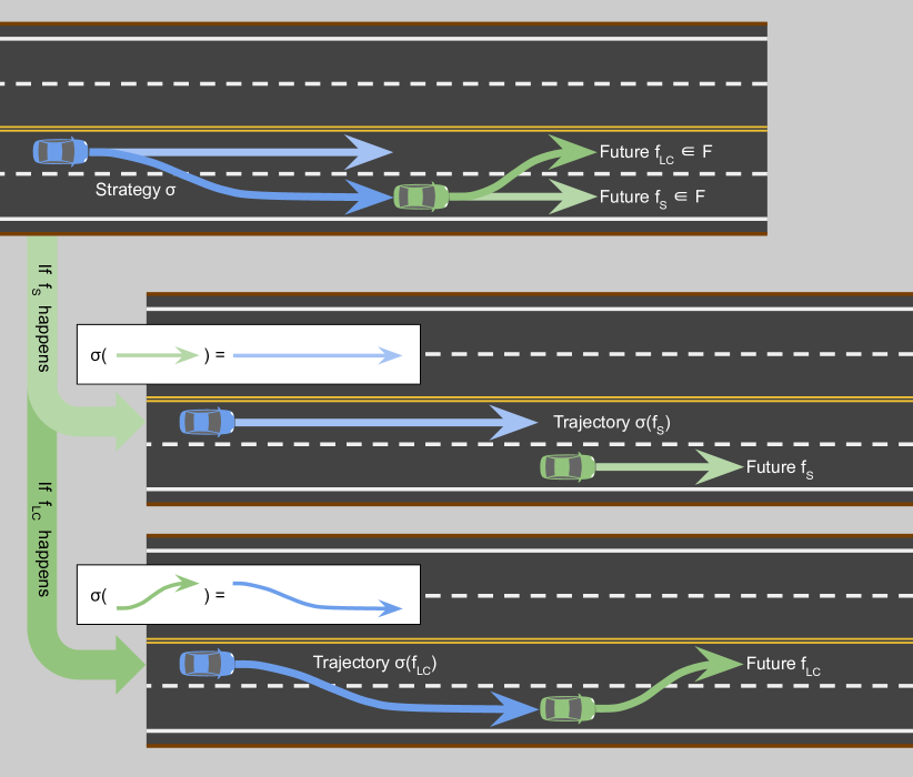
Figure 2: A strategy reacting to the two possible futures in the overtake scenario, labeled LC (for lane change) and S (for straight) respectively.

The second condition on the strategy is conceptually similar to the traditional trajectory safety:

Definition 2 (Requirement II: Reaction Safety)

A strategy $\sigma$ satisfies the Reaction Safety Requirement if the condition $C_{\sigma(f)}(t)\cap C_{f_{i}}(t)=\emptyset$ holds for all $f\in F$, all time $t\in T$ and all objects $i\in O$.

We would like to note that Requirement II is significantly weaker than the traditional safety condition $C_{\tau}(t)\cap C_{f_{i}}(t)=\emptyset$, because the former only requires each trajectory to be free of collision with its own corresponding future, rather than with all possible futures. This is the key distinction that allows the AV to avoid being stuck when the reachable sets become too spread: each situation can have its own particular solution, and the solution for one situation does not need to concern itself with handling other situations. With these two requirements, we are ready to define the safety condition based on reactions, called Comprehensive Reactive Safety (CRS).

Definition 3 (Comprehensive Reactive Safety, CRS)

A strategy $\sigma$ is said to satisfy CRS if it satisfies both Requirement I and Requirement II.

CRS guarantees safety in the sense of the following theorem, which is our main result:

Theorem 1 (Reactive Driving by a CRS Strategy is Safe)

Consider an autonomous driving system equipped with a strategy $\sigma$ satisfying CRS at time $0$. At any future time $t\in T$, the system would have observed the motion of each object over time $[0,t-\delta]$; let the motion of object $i$ so far be denoted by $m_{i}:[0,t-\delta]\to X$ for each $i\in O$. If the system executes trajectory $\sigma(f)$ for any future $f\in F$ that is compatible with the observed motions so far, that is, $f$ satisfying $f_{i}(t^{\prime})=m_{i}(t^{\prime}),\forall t^{\prime}\in[0,t-\delta],\forall i\in O$, then the system is safe from collision with any object.

Proof:

Among all the possible futures in $F$, one particular $f^{*}$ will be the one eventually occurring in reality. According to Requirement II, if the system executes $\sigma(f^{*})$ over $T$, it is safe from collisions. At any time $t\in T$, all futures $f$ compatible with observed motions $m_{i}$ so far, including $f^{*}$, are identical up to time $t-\delta$ by definition. According to Requirement I, their corresponding strategy trajectories $\sigma(f)$, including $\sigma(f^{*})$, are identical up to time $t$. Therefore, executing $\sigma(f^{*})$ is equivalent to executing the $\sigma(f)$ for any compatible $f$ for all $t\in T$, which is what the system does. ∎

Once the planner successfully plans or verifies a strategy by CRS, it has a recipe to avoid collisions, even though it does not specify a particular trajectory for the controller to follow. As long as the AV keeps observing the environment and executing the corresponding reactions in a timely manner, it will be safe from collisions, while enjoying the extra freedom not available in a traditional trajectory-based framework.

III-B Reactive ILQR

In the previous section we presented a novel safety condition that eliminates the requirement of conservatively avoiding all reachable sets. However, implementing such a framework in practice is challenging, due to the transition from trajectories to strategies. In this section, we present a practical algorithm in an attempt to leverage the flexibility of CRS in the familiar Iterative Linear Quadratic Regulator (ILQR) framework. The resulting algorithm, called Reactive ILQR, outputs CRS-worthy strategies, instead of trajectories. As an early exploration of strategy planners in lieu of trajectory planners, we focus on the necessary changes in the planner such as the representation of strategy, and keep the supporting components such as prediction and decision as simple as possible, while noting that investigation of those areas could be interesting research directions.

III-B1 Strategy as a tree of trajectories

Requirement I dictates that all trajectories in a strategy share some prefixes, some longer than others depending on how early their corresponding futures diverge. This naturally suggests a representation of strategy as a tree of trajectories, with the depth direction being time. Two trajectories sharing a prefix up to time $t$ is stored as a tree with the trunk corresponding to the common prefix segment over time $[0,t]$, and the two branches to the two different suffix segments over time $(t,t_{end}]$. Similarly, the futures $F$ are represented as a tree as well.

III-B2 Strategy branching according to future branching

Since the strategy’s trajectory $\sigma(f)$ is allowed to be different for each future $f$, it follows that the strategy should branch whenever the future branches, or in other words, the strategy tree should have the same topology as the future tree, in general. Per Requirement I, the branching point on the strategy tree must not be earlier than its counterpart on the future tree plus $\delta$, but it can be later than that, as some situations do not require immediate reactions. For simplicity, we trivially branches the strategy at time $\delta$ after each future branching point, in which case situations that do not require different reactions will simply result in identical strategy branches.

III-B3 Strategy optimization by Reactive ILQR

Once the topology of the strategy tree is known, it can be discretized and variationally optimized, subject to the safety constraints posed by Requirement II. We temporally discretize the strategy tree at a fixed time step $\Delta t$ (for example, $0.1s$) into a number of points referenced by a symbol $k$. Unlike the step index in the original ILQR, $k$ here is an identifier for a point in the strategy tree, each with a time $t(k)$ that is not necessarily unique, because multiple branches from the same parent have the same time values. The root is the only point with time 0: $t(root)=0$. Each point $k$ (except for the root) always has one unique parent point $p(k)$ which is its immediate previous step: $t(k)=t(p(k))+\Delta t$. Each point $k$ (except for the leaf points at the end of the horizon) also has one or more child points $c(k)=\{j|p(j)=k\}$ which are its immediate next steps: $t(j)=t(k)+\Delta t,\forall j\in c(k)$. A partial order $\prec$ can be naturally defined for points on a same path from the root; for example, $k\prec j$ if $k$ is an ancestor of $j$. Most points have exactly one child though, because branching occurs sparsely. Branching points segment the tree into a number of linear chunks, each a trajectory segment containing a number of points, ending with one having multiple children pointing to the subsequent branch chunks. Extending the ILQR algorithm to work with such a tree topology leads to a new algorithm we call Reactive ILQR, detailed below.

When considered in isolation, each segment is just a linear trajectory sequence that ILQR can be applied on straightforwardly. The only tricky part is that the value function parameters (such as gradients and Hessians) in the backward pass and the optimal states and controls in the forward pass need to be propagated across branching points where temporally adjacent trajectory segments meet. Concretely, given the AV state transition function $g_{k}$ and the cost function $l_{k}$ dictated by the application (potentially varying with $k$), the optimal control $\mathbf{u}^{*}$ (and the associated states $\mathbf{x}^{*}$) on a strategy tree $\sigma$ is given by the following optimization:

$$\mathbf{x}^{*},\mathbf{u}^{*} =\underset{\mathbf{x},\mathbf{u}}{\arg\min}\sum_{k}w_{k}l_{k}(\mathbf{x}_{k},\mathbf{u}_{k}),$$ (1)

$$\mathrm{s.t.} \mathbf{x}_{k} =g_{k}(\mathbf{x}_{p(k)},\mathbf{u}_{k}),$$ (2)

$$\mathbf{x}_{root} =\mathbf{x}_{0},$$ (3)

$$h_{k}(\mathbf{x}_{k}) \geq 0,$$ (4)

where $\mathbf{x}_{0}$ is the current AV state, $h_{k}$ is a collision constraint enforcing Requirement II (discussed later), and $w_{k}$ is a weight factor normalizing the contribution across sibling branches with $w_{k}=\sum_{i\in c(k)}w_{i}$. One could treat these weights as probabilities to bias the solution towards certain outcomes (futures); for simplicity we distribute the weights evenly across all sibling branches at each branching point by setting $w_{k}=\frac{1}{|c(p(k))|}w_{p(k)}$, and $w_{root}=1$.

The (negative) value function $v_{k}$ (also known as the cost-to-go function) at point $k$ on the tree topology is given by

$$v_{k}(\mathbf{x}_{k})=\min_{\{\mathbf{u}_{j}|j\succ k\}}\sum_{j\succ k}w_{j}l_{j}(\mathbf{x}_{j},\mathbf{u}_{j}),$$ (5)

with the following recursion (the Bellman equation):

$$v_{k}(\mathbf{x}_{k})$$ (6)

$$=\min_{\{\mathbf{u}_{j}|j\succ k\}}\sum_{j\in c(k)}\left(w_{j}l_{j}(\mathbf{x}_{j},\mathbf{u}_{j})+\sum_{i\succ j}w_{i}l_{i}(\mathbf{x}_{i},\mathbf{u}_{i})\right)$$ (7)

$$=\sum_{j\in c(k)}\left(\min_{\mathbf{u}_{j}}w_{j}l_{j}(g_{j}(\mathbf{x}_{k},\mathbf{u}_{j}),\mathbf{u}_{j})+v_{j}(g_{j}(\mathbf{x}_{k},\mathbf{u}_{j}))\right).$$ (8)

ILQR approximates the value function with a quadratic form by its Hessian and gradient, a form maintained inductively by (8) provided that $g_{k}$ and $l_{k}$ are in turn approximated linearly and quadratically respectively. This accomplishes the extension of ILQR to a tree topology. In general, each branching in the strategy tree doubles the number of variables to be optimized after the branching point, so the computation cost on a Y-shaped strategy will be between 1x and 2x of that on a linear trajectory. More branching will further increase the computation cost, but in the vast majority of urban driving scenarios, there is no more than one object of immediate concern, so the ILQR solver for strategy trees is still highly efficient.

The last ingredient in Reactive ILQR is the collision constraints $h_{k}$ in (4). For each point $k$, its constraint $h_{k}$ only needs to rule out collisions with the futures corresponding to this point:

$$h_{k}(\mathbf{x}_{k})=\min_{f\in\phi(k),i\in O}d(C_{f_{i}}(t(k)),\mathbf{x}_{k}),$$ (9)

where operator $d$ computes the Euclidean distance between the collision volumes of the AV and an object, and $\phi(k)=\{f|f\in F,k\in\sigma(f)\}$ is the set of futures corresponding to point $k$, which can be obtained as the strategy tree is built according to the structure of the future tree. Once constructed, the constraints $h_{k}$ can be enforced in the optimization problem (1-4) with methods like Constrained ILQR.

IV EXPERIMENTS

The proposed Reactive ILQR algorithm is quantitatively evaluated in a few representative scenarios. As a baseline, we implement a non-reactive CILQR planner that computes a single trajectory to avoid all reachable sets. For both planners, the predicted reachable sets are the same. For simplicity and comparability, the prediction module is a heuristic kinematic predictor that outputs an uncertainty box on each time step to represent the reachable set, and no explicit behavior decision module (making decisions like “pass” or “yield”) is used. Time discretization is at a resolution of $\Delta t=0.1s$, and the sensing delay $\delta$ is set to $0.1s$. The planners are run in a proprietary simulator with HD maps set up, objects spawned and scripted, and evaluation metrics (such as collision and interaction outcome) calculated to each scenario specification, detailed below.

The scenarios described below (Figure 3) have infinitely many variations, parameterized by manually-designed parameters such as the initial positions of the interacting vehicles and the actions they take (e.g. whether to brake). For each scenario, we run both RILQR and the baseline CILQR on 100 samples in the scenario variation space, and compare aggregate statistics to evaluate their capabilities in staying safe and making progress. For the crossing and unprotected turn scenarios, the 100-sample batch experiments are then repeated 10 times to obtain the error bars on the statistics.

Figure 3: The setup of the four representative scenarios. The blue vehicle is the AV while the green vehicles are the BVs.

IV-A Intersection crossing

A common interaction that demands the AV to consider multiple possible actions of the other vehicle (referred to as the background vehicle, BV) is the intersection crossing scenario. Both the AV and the BV approach an uncontrolled intersection from different directions, and at least one of them must yield to avoid collisions. In our setup the BV is spawned at a location equidistant to the intersection as the AV, and scripted to either maintain its speed at $10m/s$ (which is also the AV’s initial and target speed) or slow down before reaching the intersection by braking at $1.5m/s^{2}$ for two seconds. Although the BV’s behavior is limited to the binary choice of braking or not braking in any variation of this scenario, the reachability analysis at any moment cannot assume the BV will not vary its acceleration, and as a result the reachable boxes of both choices overlap each other forming a continuous prohibited zone for a non-reactive planner, making it unable to proceed in either case, manifested as an excessive inclination to yield. A reactive planner, on the other hand, would be able to plan a strategy that yields when the BV does not brake, and passes when the BV brakes. Simulations sampling the variation of initial longitudinal positions and initial speeds of the AV and BV confirm this conjecture: while both RILQR and the baseline ensure that no collisions occur, the AV driven by RILQR is able to pass the BV much more often (Table I). Figure 4 shows the behavior of RILQR in a typical variation.

Planner	Crossing	Unprotected left turn
Baseline	$11.6\%\pm 3.6\%$	$33.8\%\pm 4.9\%$
RILQR	$35.6\%\pm 5.3\%$	$57.4\%\pm 5.3\%$

TABLE I: Passing percentages in the intersection crossing (Fig. 4) and unprotected left turn (Fig. 5) scenarios. Passing is defined as moving through the intersection at an earlier time than the other vehicle, and yielding the opposite. RILQR achieves a higher passing ratio because it does not conservatively avoid all potential BV actions which is only possible through excessive yielding.

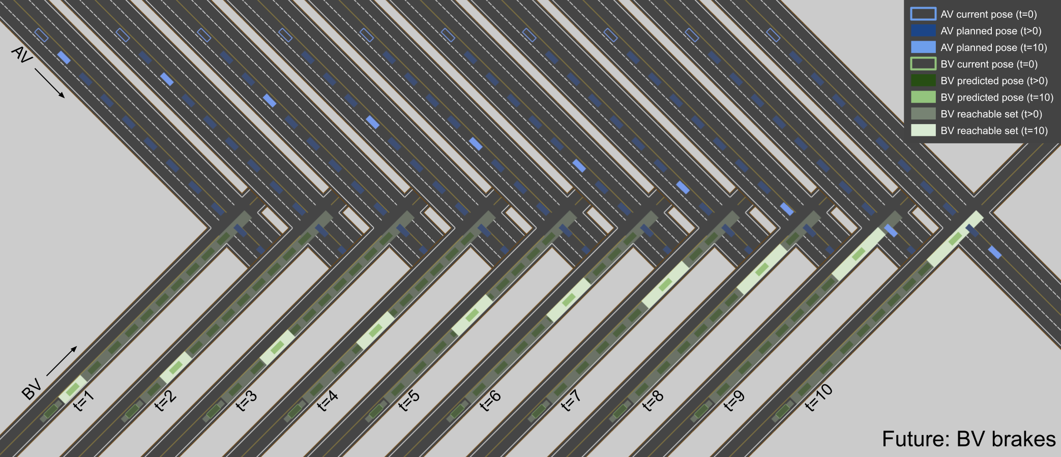
Figure 4: RILQR strategy in a crossing scenario variation, at a planning iteration 3 seconds into the simulation. The future where the BV brakes (and thus the AV proceeds) is shown on the top; the future where the BV does not brake (and thus the AV yields) is shown on the bottom. Each frame in the horizontal sequence advances one second into the future, highlighted in bright blue (AV pose in the strategy) and green (BV pose in the prediction), with the brighter green areas depicting the reachable sets. Note that all of these are planned at a single simulation time $t_{sim}=3s$ which is before the potential braking time of the BV, so the planner cannot know whether the BV ends up braking or not in this particular scenario variation, nor does it require the knowledge because its strategy is ready for both.

IV-B Unprotected left turn

A similar situation arises when the BV comes from the opposite direction and intends to make an unprotected left turn. Although the right of way rule generally requires the vehicle making the turn to ensure that doing so does not obstruct the surrounding traffic, violations to this rule occur frequently enough in reality that the AV must be prepared to yield when the BV recklessly proceeds with the turn. As with the intersection crossing scenario, RILQR improves the pass ratio without introducing collisions. Figure 5 illustrates a typical variation in this scenario.

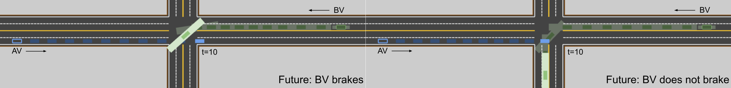
Figure 5: RILQR strategy in an unprotected left turn scenario variation, at a planning iteration 3 seconds into the simulation. The color scheme is the same as crossing (Fig. 4).

IV-C Overtake on a multi-lane road

As previously discussed, the side-passing scenario (Fig. 1) requires the fast vehicle to understand that although the slow vehicle could potentially change lanes and thus could appearing in either lane in the future, an appropriate reaction is always available to complete the overtake. We design a scenario where the BV, moving at a slow $1m/s$ in the right lane, may initiate a lane change to the left at a random moment, provided that the AV is not imminently passing it (in which case the lane change is considered malicious; see the footnote in Section I). The AV starts in the left lane, and has a target speed of $10m/s$. Experiments show that the baseline planner invariably fails to overtake as expected (see Section I), while RILQR succeeds 100% of the time without any collision (Table II).

Planner	Overtake success	BV lane change	AV average speed
Baseline	$0\%$	$66\%$	$5.02m/s$
RILQR	$100\%$	$42\%$	$9.94m/s$

TABLE II: Statistics in the overtake scenario (Fig. 6). Overtake success is defined as the AV being longitudinally ahead at the end of the simulation. RILQR is able to overtake because it can find a way forward whether the BV changes lane or not.

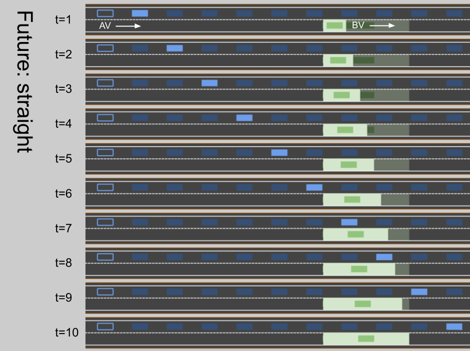
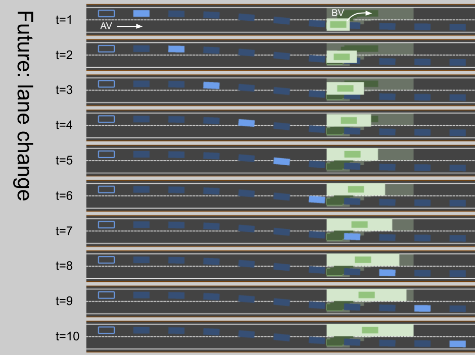
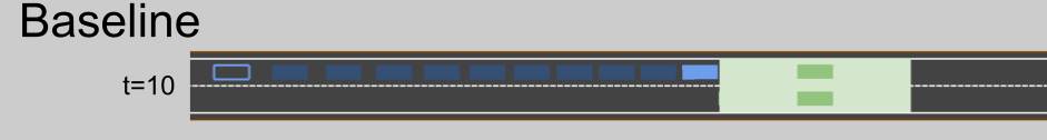
Figure 6: RILQR strategy in an overtake scenario variation, at a planning iteration 4 seconds into the simulation. For comparison, the behavior of the baseline planner is also included at the bottom.

IV-D Merge

To stress-test RILQR in a complex interaction situation, we set up a merge challenge scenario where the AV approaches a lane merge into the left lane with continuous traffic of tightly spaced BVs, each traveling at $10m/s$ (equal to the AV’s default initial and target speed) and may either brake or maintain speed before arriving at the merge point, just like in the crossing scenario. In addition to each BV’s individual braking action, also varied are the AV initial speed and longitudinal position, to cover the full range of possible initial configurations. The scripted motions of the BV themselves could sometimes be unrealistic or malicious, especially the “pincer movement” in certain cases where a BV in the front brakes and another one right behind it does not brake, and as a result both RILQR and the baseline encountered collisions, but RILQR does achieve a lower collision rate, and, more importantly, a generally more advanced post-merge position in the row of BVs (Table III), able to complete the merge before the fourth BV passes $88\%$ of the time compared to $30\%$ with the baseline planner, and able to slot in between the first two BVs twice as often. Since the average initial position of the AV is longitudinally between the first and the second BV, this means the behavior of RILQR, instead of being overly aggressive, is probably closer to a more smooth and fluid merging sequence that avoids the harsh braking needed to find a merge spot behind latter BVs.

		Post-merge position in the BV queue
Planner	Collision	Before 1	1-2	2-3	3-4	After 4
Baseline	$16\%$	$1\%$	$23\%$	$6\%$	$0\%$	$70\%$
RILQR	$5\%$	$1\%$	$44\%$	$31\%$	$12\%$	$12\%$

TABLE III: Statistics in the merge challenge (Fig. 7). The numbers in the post-merge position columns are BV indices. For example, if the AV merged between the 1st and 2nd BV by the end of the scenario, it is counted as “1-2”, and so on.

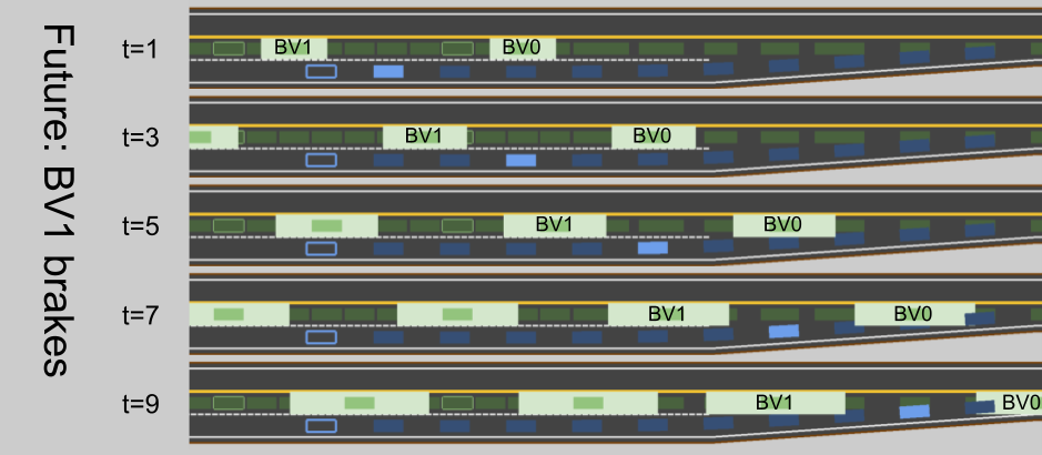
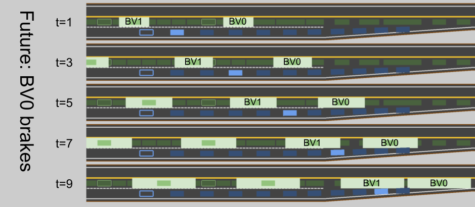
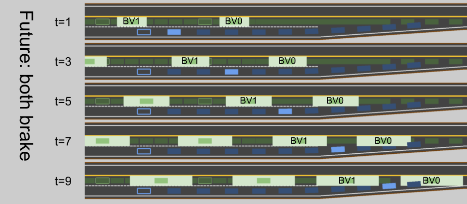
Figure 7: RILQR strategy in a merge scenario variation, at a planning iteration 4 seconds into the simulation. Two objects (BV0 and BV1) branch off at different times resulting in four distinct futures, and thus four trajectories in the strategy. The top two trajectories are nearly identical, both merging between the opening BV0 and BV1. The bottom-right trajectory also finds the same opening, although overall slower because BV0 brakes. The bottom-left trajectory cannot merge and has to slow down because BV1’s braking eliminates the opening.

V CONCLUSIONS

In this work, we call for a paradigm shift in the treatment of safety in motion planning for autonomous driving. Instead of basing the safety condition on the static knowledge of the currently known environment, we advocate defining safety with consideration of how the environment will change in the future, and how the autonomous driving system will react, because that is what the system does in the general case. This in turn necessitates a shift in the planner architecture, from planning trajectories to planning strategies. We outline a safety framework in this context, called CRS, and give an implementation, called RILQR. The effectiveness of both is demonstrated in simulations.

This paradigm shift, especially the new strategy planner architecture, opens up many interesting avenues of research. In particular, the module that partitions the predicted motions of objects from continuous distributions of trajectories into discrete branches of a strategy plays a crucial decision-making role because it essentially determines what motions of the objects need different reactions from the AV, and research on this topic is scarce. Another example is the question of how to register the current strategy against the potentially topologically incompatible strategy from the previous planning iteration, which is often needed to ensure smoothness across plan handovers in the controller. We believe the concept of strategy planners is worthy of more investigation effort, and more insight about the planning problem itself may be uncovered in the process.

References

- [1] D. Rojas-Rueda, M. J. Nieuwenhuijsen, H. Khreis, and H. Frumkin, “Autonomous vehicles and public health,” Annual review of public health, vol. 41, pp. 329–345, 2020.
- [2] WaymoLLC, “Waymo safety report,” accessed: 2/21/2022. [Online]. Available: https://waymo.com/safety/
- [3] M. Althoff and J. M. Dolan, “Online verification of automated road vehicles using reachability analysis,” IEEE Transactions on Robotics, vol. 30, no. 4, pp. 903–918, 2014.
- [4] C. Pek, S. Manzinger, M. Koschi, and M. Althoff, “Using online verification to prevent autonomous vehicles from causing accidents,” Nature Machine Intelligence, vol. 2, no. 9, pp. 518–528, 2020.
- [5] A. Li, L. Sun, W. Zhan, M. Tomizuka, and M. Chen, “Prediction-based reachability for collision avoidance in autonomous driving,” in 2021 IEEE International Conference on Robotics and Automation (ICRA). IEEE, 2021, pp. 7908–7914.
- [6] S. Shalev-Shwartz, S. Shammah, and A. Shashua, “On a formal model of safe and scalable self-driving cars,” arXiv preprint arXiv:1708.06374, 2017.
- [7] M. McNaughton, C. Urmson, J. M. Dolan, and J.-W. Lee, “Motion planning for autonomous driving with a conformal spatiotemporal lattice,” in 2011 IEEE International Conference on Robotics and Automation. IEEE, 2011, pp. 4889–4895.
- [8] J. Levinson, J. Askeland, J. Becker, J. Dolson, D. Held, S. Kammel, J. Z. Kolter, D. Langer, O. Pink, V. Pratt, et al., “Towards fully autonomous driving: Systems and algorithms,” in 2011 IEEE intelligent vehicles symposium (IV). IEEE, 2011, pp. 163–168.
- [9] W. Xu, J. Wei, J. M. Dolan, H. Zhao, and H. Zha, “A real-time motion planner with trajectory optimization for autonomous vehicles,” in 2012 IEEE International Conference on Robotics and Automation. IEEE, 2012, pp. 2061–2067.
- [10] J. Ziegler, P. Bender, M. Schreiber, H. Lategahn, T. Strauss, C. Stiller, T. Dang, U. Franke, N. Appenrodt, C. G. Keller, et al., “Making bertha drive—an autonomous journey on a historic route,” IEEE Intelligent transportation systems magazine, vol. 6, no. 2, pp. 8–20, 2014.
- [11] Y. Chen, H. Peng, and J. Grizzle, “Obstacle avoidance for low-speed autonomous vehicles with barrier function,” IEEE Transactions on Control Systems Technology, vol. 26, no. 1, pp. 194–206, 2017.
- [12] S. Boyd, S. P. Boyd, and L. Vandenberghe, Convex optimization. Cambridge university press, 2004.
- [13] D. P. Bertsekas, Constrained optimization and Lagrange multiplier methods. Academic press, 2014.
- [14] X. Qian, F. Altché, P. Bender, C. Stiller, and A. de La Fortelle, “Optimal trajectory planning for autonomous driving integrating logical constraints: An miqp perspective,” in 2016 IEEE 19th international conference on intelligent transportation systems (ITSC). IEEE, 2016, pp. 205–210.
- [15] J. Chen, W. Zhan, and M. Tomizuka, “Constrained iterative lqr for on-road autonomous driving motion planning,” in 2017 IEEE 20th International Conference on Intelligent Transportation Systems (ITSC). IEEE, 2017, pp. 1–7.
- [16] ——, “Autonomous driving motion planning with constrained iterative lqr,” IEEE Transactions on Intelligent Vehicles, vol. 4, no. 2, pp. 244–254, 2019.
- [17] W. Li and E. Todorov, “Iterative linear quadratic regulator design for nonlinear biological movement systems.” in ICINCO (1). Citeseer, 2004, pp. 222–229.
- [18] E. Todorov and W. Li, “A generalized iterative lqg method for locally-optimal feedback control of constrained nonlinear stochastic systems,” in Proceedings of the 2005, American Control Conference, 2005. IEEE, 2005, pp. 300–306.
- [19] D. Althoff, M. Althoff, and S. Scherer, “Online safety verification of trajectories for unmanned flight with offline computed robust invariant sets,” in 2015 IEEE/RSJ International Conference on Intelligent Robots and Systems (IROS). IEEE, 2015, pp. 3470–3477.
- [20] P. F. Orzechowski, A. Meyer, and M. Lauer, “Tackling occlusions & limited sensor range with set-based safety verification,” in 2018 21st International Conference on Intelligent Transportation Systems (ITSC). IEEE, 2018, pp. 1729–1736.
- [21] J. Gao, C. Sun, H. Zhao, Y. Shen, D. Anguelov, C. Li, and C. Schmid, “Vectornet: Encoding hd maps and agent dynamics from vectorized representation,” in Proceedings of the IEEE/CVF Conference on Computer Vision and Pattern Recognition, 2020, pp. 11 525–11 533.
- [22] H. Zhao, J. Gao, T. Lan, C. Sun, B. Sapp, B. Varadarajan, Y. Shen, Y. Shen, Y. Chai, C. Schmid, et al., “Tnt: Target-driven trajectory prediction,” arXiv preprint arXiv:2008.08294, 2020.
- [23] M. Liang, B. Yang, R. Hu, Y. Chen, R. Liao, S. Feng, and R. Urtasun, “Learning lane graph representations for motion forecasting,” in European Conference on Computer Vision. Springer, 2020, pp. 541–556.
- [24] I. M. Mitchell, A. M. Bayen, and C. J. Tomlin, “A time-dependent hamilton-jacobi formulation of reachable sets for continuous dynamic games,” IEEE Transactions on automatic control, vol. 50, no. 7, pp. 947–957, 2005.
- [25] B. Vanholme, D. Gruyer, B. Lusetti, S. Glaser, and S. Mammar, “Highly automated driving on highways based on legal safety,” IEEE Transactions on Intelligent Transportation Systems, vol. 14, no. 1, pp. 333–347, 2012.
- [26] Y. Pan, Q. Lin, H. Shah, and J. M. Dolan, “Safe planning for self-driving via adaptive constrained ilqr,” in 2020 IEEE/RSJ International Conference on Intelligent Robots and Systems (IROS). IEEE, 2020, pp. 2377–2383.