Generating Counterfactual Hard Negative Samples for Graph Contrastive Learning

Abstract.

Graph contrastive learning has emerged as a powerful unsupervised graph representation learning tool. The key to the success of graph contrastive learning is to acquire high-quality positive and negative samples as contrasting pairs to learn the underlying structural semantics of the input graph. Recent works usually sample negative samples from the same training batch with the positive samples or from an external irrelevant graph. However, a significant limitation lies in such strategies: the unavoidable problem of sampling false negative samples. In this paper, we propose a novel method to utilize Counterfactual mechanism to generate artificial hard negative samples for Graph Contrastive learning, namely CGC. We utilize a counterfactual mechanism to produce hard negative samples, ensuring that the generated samples are similar but have labels that differ from the positive sample. The proposed method achieves satisfying results on several datasets. It outperforms some traditional unsupervised graph learning methods and some SOTA graph contrastive learning methods. We also conducted some supplementary experiments to illustrate the proposed method, including the performances of CGC with different hard negative samples and evaluations for hard negative samples generated with different similarity measurements. The implementation code is available online to ease reproducibility.

1. Introduction

Graph contrastive learning (GCL) (Velickovic et al., 2019; Qiu et al., 2020; You et al., 2020; Zhu et al., 2021; Hassani and Ahmadi, 2020; Yang et al., 2022; Sun et al., 2020) has emerged as a powerful learning paradigm for unsupervised graph representation learning. Inspired by the widely adopted contrastive learning framework in computer vision (CV) (Wu et al., 2018; He et al., 2020) and natural language processing (NLP) (Clark et al., 2020), GCL leverages the advanced representation learning capabilities of graph neural networks (GNNs) (Kipf and Welling, 2017; Xu et al., 2019; Jin et al., 2022; Fan et al., 2022) and tries to distil high-quality representative graph embeddings of an input graph via comparing the differences and similarities among augmented graphs (i.e., positive and negative samples) derived from the original input.

The key to a successful GCL method is to derive high-quality contrasting samples from the original input graph. To date, various kinds of methods to generate positive samples are proposed, for example, graph augmentations-based approaches (You et al., 2020; Zhu et al., 2021) and multi-view sample generation (Hassani and Ahmadi, 2020; Yang et al., 2022), which have been becoming dominant and achieved satisfying performance. Despite this progress, especially in manipulating positive pairs, far less attention has been given to obtaining negative samples (Robinson et al., 2021). Compared to positive samples in contrastive learning, negative sampling is more challenging and non-trivial(Robinson et al., 2021). Existing methods of negative sample acquisition mainly follow traditional sampling techniques, which may encounter the deficiency caused by unnoticeable false negative samples (Xia et al., 2021). For instance, GraphCL (You et al., 2020) samples other graphs as the negative samples from the same training batch where the target graph comes from. Such an approach does not guarantee that the sampled negative graphs are true. GCC (Qiu et al., 2020) samples negative graphs from an external graph based on the assumption that common graph structural patterns are universal and transferable across different networks. However, this assumption neither has any theoretical guarantee nor has been validated by empirical study(Qiu et al., 2020). To alleviate the impact caused by false-negative samples, debiasing treatment has been introduced to current graph contrastive learning methods (Xia et al., 2021; Zhao et al., 2021). The idea of these debiased graph contrastive learning methods is to estimate the probability of whether a negative sample is false. Based on this, some negative samples with low confidence will be discarded or treated with lower weights in the contrastive learning phase. Nevertheless, a typical major limitation of both GCL and the debiasing-based variants is still evident - most of these sampling strategies are stochastic and random. In other words, current methods do not guarantee the quality of the sampled negative pairs.

To address the previously mentioned problems, we first name the high-quality negative samples as hard negative samples and give corresponding definitions. According to (Robinson et al., 2021), a hard negative sample is a data instance whose label differs from that of the target data, and its embedding is similar to that of the target data. Considering the limitations of sampling-based strategies discussed previously, we argue that a strictly constrained generative process must be imposed to guarantee the quality of the negative samples (a.k.a. generating hard negative samples). Inspired by counterfactual reasoning (Li et al., 2022), a fundamental reasoning pattern of human beings, which helps people to reason out what minor behaviour changes may result in considerable differences in the final event outcome. We intuitively came up with the idea that the hard negative sample generation should apply minor changes to the target graph and finally can obtain a perturbed graph whose label is strictly different from the original graph.

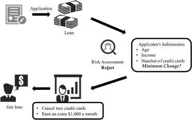
Figure 1. An illustrative example about a counterfactual explanation. Someone wants to apply for a loan, but the application is rejected after a risk assessment from the financial institution. Many factors are related to the final decision, such as the applicant’s age, income, and number of credit cards. The minimum change the applicant needs to make to get the loan is earning an extra $1,000 per month or cancelling two credit cards.

An illustrative example about a counterfactual explanation. Someone wants to apply for a loan, but the application is rejected after a risk assessment from the financial institution. Many factors are related to the final decision, such as the applicant’s age, income, and number of credit cards. The minimum change the applicant needs to make to get the loan is earning an extra $1,000 per month or cancelling two credit cards.

To this end, we propose generating two types of hard negative samples via perturbations to the original input graph: proximity perturbed graphs and feature-masked graphs. It is worth noting that these two types of generation processes will be adaptively conducted and constrained by sophisticating similarity-aware loss functions. However, this process is still challenging and non-trivial. We believe there are two significant challenges. First, in graph perturbation and feature masking, how to measure a generated sample is hard? To solve the problem, we first design two indication matrices demonstrating the changes made to the graph structure and feature space. Then, different matrix norms are applied to indication matrices to reflect how much perturbation has been made. We will minimise the calculated matrix norms such that the perturbation applied to the original graph to generate negative samples is as minor as possible. In this case, the generated samples would be similar to the original graph in proximity and feature space. By adopting matrix norms, we can quantify the perturbation and ensure that the generated samples are hard ones. After formulating a constraint that forces the generated samples to be hard to distinguish from the target in proximity and feature space, the second challenge is how to make sure the generated hard samples have different labels from the target. That is to say, how can we ensure the generated hard samples are true negative? We first feed the target graph and the generated samples into a graph classifier to achieve that. The classifier will then output the probability distributions of the classes to which the target graph and the generated samples belong. Following the counterfactual mechanism, an objective measuring the differences between the classifier’s outputs for the target graph and that for the generated samples is applied and minimised. Specifically, the similarities between the predicted probability distributions are minimised via monitoring the KL divergence. With the two objectives described above, we can generate high-quality hard negative samples with proper and reasonable constraints.

We propose a counterfactual-inspired generative method for graph contrastive learning to obtain hard negative samples. It explicitly introduces constraints to ensure the generated negative samples are true and hard, eliminating the random factors in current negative sample acquiring methods in GCL methods. Furthermore, once the generation procedure is finished, we do not need further steps (e.g., debiasing) to process the acquired samples. The contributions of our work are summarized as follows:

• We propose a novel adaptively graph perturbation method, CGC, to produce high-quality hard negative samples for the GCL process.

• We innovatively introduce the counterfactual mechanism into the GCL domain, leveraging its advantages to make the generated negative samples be hard and true. Due to the successful application of the counterfactual mechanism in our work, there is potential feasibility of conducting the counterfactual reasoning to explain GCL models.

• We conducted extensive experiments to demonstrate the proposed method’s effectiveness and properties, which achieved state-of-the-art performances compared to several classic graph embedding methods and some novel GCL methods.

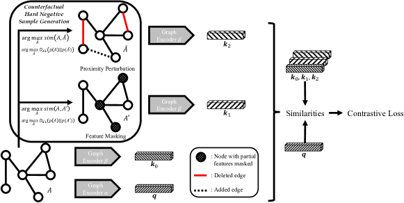
Figure 2. The overview of CGC. We first conduct counterfactual hard negative sample generation to acquire a proximity-perturbed and feature-masked sample. Then, the target and the two generated hard negative samples will be fed into the graph contrastive learning module to learn graph embeddings.

The overview of CGC. We first conduct counterfactual hard negative sample generation to acquire a proximity-perturbed and feature-masked sample. Then, the target and the two generated hard negative samples will be fed into the graph contrastive learning module to learn graph embeddings.

2. Related Work

This section briefly introduces the backgrounds and research progress in two highly related areas, including counterfactual reasoning mechanisms and graph contrastive learning.

2.1. Counterfactual Reasoning Mechanism

Counterfactual reasoning is a basic way of reasoning that helps people understand their behaviours and the world’s rules (Li et al., 2022). The definition of counterfactual reasoning is given by (Pearl and Mackenzie, 2018) stating that counterfactual is a probabilistic answer to a ‘what would have happened if’ question. Many illustrative examples are provided in (Wang et al., 2021) to help understand the ideas behind counterfactual. For instance, as shown in Figure 1. Counterfactual is a kind of thinking mechanism to discover the facts that contradict existing facts and could potentially alter the outcomes of a decision-making process. There are some restrictions on counterfactuals. First, many factors could potentially affect the final results. However, counterfactuals must apply as small as possible changes to achieve such a goal. Second, counterfactuals must be feasible and reasonable. In Figure 1, the financial institution would release the loan without hesitation if the applicator earns an extra one million dollars per month. Nevertheless, the applicator cannot have such a high salary quickly. So, earning an extra one million dollars per month is not a counterfactual. A classical counterfactual method is heuristic counterfactual generation (Wachter et al., 2018), shown in Algorithm 1, where

(1) $$L(x,x^{\prime},y^{\prime},\lambda)=\lambda\overbrace{(\hat{f}(x^{\prime})-y^{\prime})^{2}}^{\text{distance in predictions}}+\underbrace{d(x,x^{\prime})}_{\text{distance in instances}},$$

and $x$ denotes the target instance, $x^{\prime}$ is counterfactual, $y^{\prime}$ represents the desired outcome, $\lambda$ is the term used to balance two distances, and $\epsilon$ denotes tolerance for the distance. This equation is the objective function of the heuristic counterfactual generation algorithm. It maximises the distances in predictions and minimises the distance between the original instance $x$ and the counterfactual $x^{\prime}$.

Algorithm 1 Heuristic counterfactual generation algorithm

  sample a random instance as the initial $x^{\prime}$

  optimise $L(x,x^{\prime},y^{\prime},\lambda)$ with $x^{\prime}$

  while $|\hat{f}(x^{\prime})-y^{\prime}|>\epsilon$ do

     increase $\lambda$ by step-size $\alpha$

     optimise $L(x,x^{\prime},y^{\prime},\lambda)$ with new $x^{\prime}$

  end while

  return  $x^{\prime}$

2.2. Graph Contrastive Learning

Recently, many researchers devoted themselves to constructing proper positive pairs to conduct graph contrastive learning. There are plenty of works describing how to generate high-quality positive pairs to conduct graph contrastive learning (Velickovic et al., 2019; Sun et al., 2020; You et al., 2020; Hassani and Ahmadi, 2020; Yang et al., 2022; Qiu et al., 2020), and indeed, they have achieved promising performances. However, works introducing how to obtain negative samples to facilitate graph contrastive learning further are scarce in the current literature. Recent works usually adopted sampling strategies to acquire negative samples. Specifically, in GraphCL (You et al., 2020), the authors proposed to sample other graphs as the negative samples from the same training batch in which the target graph is. However, under the scenario of lacking label information, the sampled graphs may have the same label as the target graph, resulting in sampling false negative graphs. Similarly, GCA and InfoGraph conducted contrastive learning at the node level. They sampled negative nodes from the neighbours of the target (Zhu et al., 2021; Sun et al., 2020). Such a strategy would also meet the false negative sample problem. Moreover, GCC was proposed to sample negative graphs from an external dataset. Undoubtedly, the external negative samples have different semantics or labels from the target graph (Qiu et al., 2020). However, such a strategy was proposed based on the hypothesis that representative graph structural patterns are universal and transferable across networks (Qiu et al., 2020). This hypothesis has not been verified that it holds among all graph datasets.

Sampling-based methods for hard negative sample generation suffer from the false negative sample problem and attract the researchers’ attention. Some recent works (Xia et al., 2021; Zhao et al., 2021) tried to address such a problem by relieving the biases existing in the negative graph sampling process. DGCL (Xia et al., 2021) found out the harder the negative sample is, the more likely a false negative sample is, and the probability of being a false negative sample is related to the similarity between the target and the sampled negative instances. The strategy DGCL adopted is straightforward to understand, reducing the weight of the negative samples that are likely to be false in the contrastive training procedure. Such a method indeed relieved the impact brought by the false negative samples. GDCL (Zhao et al., 2021) utilised graph clustering techniques to determine if a negative sample is false before feeding it into the contrastive learning process. Graph clustering is applied to the set containing the initial sampled negative instances and the target. The instances in the cluster where the target is would be discarded because they are more likely to have the same labels as the target.

Nevertheless, a typical major limitation of both GCL and the debiasing-based variants is still evident - most of these sampling strategies are stochastic and random. In other words, current methods do not guarantee the quality of the sampled negative pairs.

3. Methodology

This section will give a detailed illustration of the proposed method and the training procedure. The overview of the proposed method is illustrated in Figure 2.

3.1. Problem Definition

Given a graph $\mathcal{A}=\{\mathcal{V},\mathcal{E},\mathcal{X}\}$, where $\mathcal{V}$ denotes all the nodes, $\mathcal{E}$ represents all the edges, and $\mathcal{X}$ is the set consists of the features of all nodes. If there are $N$ nodes and the dimension of the feature is $h$, then, $\mathcal{X}\in\mathbb{R}^{N\times h}$. Our method aims to derive some negative graphs from the input graph based on counterfactual mechanisms, and a toy example is shown in Figure 3. For simplicity’s sake, in this paper, we consider the scenario where two kinds of hard negative graphs are generated, the proximity perturbed graph $\mathcal{A}^{\prime}=\{\mathcal{V},\mathcal{E}^{\prime},\mathcal{X}\}$ and the feature masked graph $\tilde{\mathcal{A}}=\{\mathcal{V},\mathcal{E},\tilde{\mathcal{X}}\}$, such that

(2) $$\mathop{\arg\max}_{\mathcal{E}^{\prime},\tilde{\mathcal{X}}}sim(\mathcal{A},\mathcal{A}^{\prime})+sim(\mathcal{A},\tilde{\mathcal{A}}),$$

(3) $$\mathop{\arg\max}_{\mathcal{E}^{\prime},\tilde{\mathcal{X}}}D_{KL}(p(\mathcal{A})||p(\mathcal{A}^{\prime}))+D_{KL}(p(\mathcal{A})||p(\tilde{\mathcal{A}})),$$

where $sim(*)$ denotes the metric to measure the similarity between two items (e.g., graph adjacency matrices, feature matrices), $D_{KL}(*)$ is the KL-Divergence (Kullback and Leibler, 1951) function, which is used to measure the similarity between two probability distributions, and $p(*)$ denotes predictor outputting the probabilities of classes to which the graph belongs. The intuition behind the two formulas is to derive hard negative graphs with different labels while forcing the derived graphs to be as similar to the original graph as possible. In other words, we want to achieve dramatic change at the semantics level with minor perturbations at the graph’s essential elements. The problem is formulated as an optimisation problem to maximise the similarities between the generated negative samples and the target in proximity and feature and force them to have different labels.

3.2. Counterfactual Adaptive Perturbation

Table 1. Statistics of four graph datasets.

Dataset	Num. of Graphs	Avg. Num. of Nodes	Avg. Num. of Edges	Node Attr. Dim.	Num. of Classes
PROTEINS_full	1,113	39.06	72.82	29	2
FRANKENSTEIN	4,337	16.90	17.88	780	2
Synthie	400	95.00	172.93	15	4
ENZYMES	600	32.63	62.14	18	6

This paper discusses two adaptive perturbation matrices: the proximity perturbation matrix and the feature masking matrix.

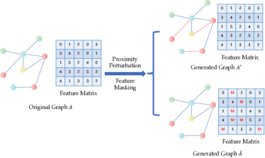
Figure 3. An example of the graphs with proximity perturbed and with features masked derived from an original graph.

A toy example about the graph with proximity perturbed and the graph with features masked derived from the original graph.

3.2.1. Proximity Perturbation

Proximity perturbation aims to change the graph structure to generate a contrasting sample. This can help the model learn the critical structural information in the original graph (You et al., 2020; Zhu et al., 2021). First, let us focus on how to conduct adaptive perturbation. To achieve the goal of adaptive perturbation, we need a trainable matrix $\mathbf{M}_{a}\in\mathbb{R}^{N\times N}$, such that

(4) $$\mathbf{A}_{a}=\mathbf{M}_{a}\times\mathbf{A},$$

where $\mathbf{A}\in\mathbb{R}^{N\times N}$ is the adjacency matrix of $\mathcal{A}$, and $\mathbf{A}_{a}$ denotes the adjacency matrix of the proximity perturbed graph $\mathcal{A}^{\prime}$. Note that we adopt matrix multiplication here instead of taking the Hadamard product since it cannot add an edge to the adjacency matrix. Moreover, values of the entries of $\mathbf{A}_{a}$ are in $\mathbb{R}^{N\times N}$, which conflict with the definition domain of the adjacency matrix, $\{0,1\}^{N\times N}$. We need an extra step such that $f:\mathbf{A}_{a}\in\mathbb{R}^{N\times N}\rightarrow\mathbf{A}^{{}^{\prime}}_{a}\in\{0,1\}^{N\times N}$. We use the following formula to conduct the mapping:

(5) $$\mathbf{A}^{{}^{\prime}}_{a}=\mathbb{I}(sigmoid(\mathbf{A}_{a})\geq\omega),$$

where $\mathbb{I}(*)$ is the indicator function, and $\omega$ is a threshold determining whether to set the entry as 1 or 0. Finally, we have the adjacency matrix for the negative sample $\mathcal{A}^{\prime}$. Consequently, a perturbed set $\mathcal{E}^{\prime}$ of edges is obtained. Though in this procedure, there is no modification made to nodes, we can adaptively discard some nodes by deleting all the edges of the nodes, which will be isolated from the generated graph after perturbation. In summary, we can utilise the proximity perturbation matrix and procedure mentioned above to simulate all the proximity perturbation methods in (You et al., 2020), including edge dropping or adding and node dropping.

3.2.2. Feature Masking

Feature masking tries to mask the original feature matrix to help the contrastive learning model obtain the critical information in the features (You et al., 2020; Zhu et al., 2021), which would determine the decisive factors in the feature domain. The whole procedure of feature masking is similar to the proximity perturbation, but there are some minor differences. First, same as the previous procedure, we need to initialize a trainable matrix $\mathbf{M}_{b}\in\mathbb{R}^{N\times h}$, which serves as a mask matrix here. We have to make sure the definition domain of it is $\{0,1\}^{N\times h}$. To achieve such a goal, we have

(6) $$\mathbf{M}^{{}^{\prime}}_{b}=\mathbb{I}(sigmoid(\mathbf{M}_{b})\geq\gamma),$$

where $\gamma$ is a threshold determining whether to mask some feature entries. To fulfil the feature masking procedure, we need to have Hadamard element-wise product between $\mathbf{M}^{{}^{\prime}}_{b}$ and $\mathcal{X}$ instead of matrix multiplication in the previous perturbation procedure:

(7) $$\tilde{\mathcal{X}}=\mathbf{M}^{{}^{\prime}}_{b}\circ\mathcal{X}.$$

Once we finish the feature masking procedure, the values of the masked features will be replaced with $0$.

After the proximity perturbation and the feature masking, two hard negative samples are acquired, which are $\mathcal{A}^{\prime}=\{\mathcal{V},\mathcal{E}^{\prime},\mathcal{X}\}$ and $\tilde{\mathcal{A}}=\{\mathcal{V},\mathcal{E},\tilde{\mathcal{X}}\}$, respectively.

3.2.3. Perturbation Measurement

Once we obtained two perturbed graphs, the issue we have to deal with next is how to ensure the generated graphs are hard negatives. As we mentioned previously, we leverage the counterfactual mechanism to solve this problem because this method naturally meets the requirements of hard negative sample generation. Both aim to output something different at the semantic level but similar at the structural level. We introduced two objectives in the Section. 3.1, and more details are given in this section.

First, we discuss maximising the similarity between the original and the perturbed graphs. This objective function tries to ensure the perturbation we made is as minor as possible. We utilise the Frobenius norm of the difference between $\mathbf{A}$ and $\mathbf{A}^{\prime}_{a}$. The smaller the Frobenius norm is, the more similar they are. The Frobenius norm of the masking matrix can measure the similarity between features. A relatively greater norm indicates that a small portion of feature entries are masked. Therefore, the similarity between $\mathcal{X}$ and $\tilde{\mathcal{X}}$ would be high. The objective is formulated as follows:

(8) $$\mathcal{L}_{s}=||\mathbf{A}-\mathbf{A}^{{}^{\prime}}_{a}||_{F}-||\mathbf{M}^{\prime}_{b}||_{F}.$$

Next, we must ensure the generated graphs are different from the original graph at the semantic level. Here, we consider the classification problem, where we minimize the similarity between probability distributions of classes between the original and the perturbed graphs. Therefore, we have

(9) $$\mathcal{L}_{c}=-D_{KL}(p(\mathcal{A}),p(\mathcal{A}^{\prime}))-D_{KL}(p(\mathcal{A}),p(\tilde{\mathcal{A}})).$$

So, the overall objective for counterfactual pre-training for hard negative sample generation is

(10) $$\mathcal{L}_{pre}=\mathcal{L}_{s}+\mathcal{L}_{c}.$$

3.3. Contrastive Learning Procedure

The counterfactual mechanism is adopted to generate hard negative samples. After that, we need to conduct graph contrastive learning between the original graph and the perturbed graphs. In this paper, we follow a simple and widely-used graph contrastive learning schema to conduct it, which is dictionary look-up method (Qiu et al., 2020), shown in Figure 2. Given an original input graph $\mathcal{A}$, two negative graphs $\mathcal{A}^{\prime}$ and $\tilde{\mathcal{A}}$, and two graph encoders, $g_{p}(\cdot)$ and $g_{n}(\cdot)$, we will have a sort of graph embeddings: $\mathbf{q}=g_{p}(\mathcal{A})$, $\mathbf{k}_{+}=\mathbf{k}_{0}=g_{n}(\mathcal{A})$, $\mathbf{k}_{1}=g_{n}(\mathcal{A}^{\prime})$, and $\mathbf{k}_{2}=g_{n}(\tilde{\mathcal{A}})$. Specifically, the target graph will be encoded by both graph encoders, and $g_{n}(\cdot)$ will only be used to encode the generated hard negative samples. Dictionary look-up method here tries to look up a single key (denoted by $\mathbf{k}_{+}$) that $\mathbf{q}$ matches in $\mathbb{K}$. Let $\mathbf{q}$ denotes the query key and $\mathbb{K}=\{\mathbf{k}_{0},\mathbf{k}_{1},\mathbf{k}_{2}\}$ be the dictionary, we take InfoNCE in (van den Oord et al., 2018) to formulate contrastive learning procedure. So, we have the objective for the graph contrastive learning phase:

(11) $$\mathcal{L}_{contra}=-\log\frac{\exp(sim(\mathbf{q},\mathbf{k}_{+})/\tau)}{\sum^{|\mathcal{K}|-1}_{t=0}\exp(sim(\mathbf{q},\mathbf{k}_{t})/\tau)},$$

where $\tau$ is the temperature hyperparameter.

After finishing the two training phases, including counterfactual mechanism-based hard negative samples generation and graph contrastive learning, we can obtain the trained embeddings of all nodes and graphs. The graph embeddings will be fed into a downstream prediction model to conduct graph classification tasks and evaluate the trained embeddings’ quality.

4. Experiment

Table 2. Comparison experimental results. F1-micro and F1-macro scores (%) with standard deviations are listed above.

	PROTEINS_full		FRANKENSTEIN		Synthie		ENZYMES
	F1-Micro	F1-Macro	F1-Micro	F1-Macro	F1-Micro	F1-Macro	F1-Micro	F1-Macro
RandomWalk	-	-	57.97(std 2.15)	57.45(std 1.92)	18.50(std 4.06)	16.86(std 3.58)	-	-
ShortestPath	70.88(std 4.91)	69.88(std 4.99)	62.39(std 1.95)	59.81(std 2.02)	50.75(std 9.69)	47.32(std 9.86)	27.83(std 6.37)	27.18(std 5.93)
GL	69.89(std 3.25)	68.57(std 3.43)	61.26(std 2.85)	53.94(std 2.46)	52.50(std 10.49)	50.24(std 10.37)	31.67(std 7.03)	30.02(std 7.13)
WL	72.32(std 3.11)	71.36(std 3.41)	-	-	-	-	37.83(std 4.95)	36.42(std 5.78)
sub2vec	70.17(std 2.06)	66.26(std 0.44)	54.97(std 1.80)	46.83(std 4.00)	29.75(std 4.67)	22.07(std 3.75)	19.67(std 3.64)	13.34(std 4.33)
graph2vec	68.65(std 3.45)	64.16(std 5.00)	61.70(std 3.04)	59.68(std 0.22)	54.25(std 0.62)	35.17(std 0.26)	25.67(std 4.84)	22.41(std 5.04)
InfoGraph	71.61(std 4.67)	70.48(std 5.06)	63.57(std 2.12)	62.95(std 2.20)	54.5(std 8.05)	54.17(std 7.87)	38.33(std 7.03)	37.07(std 6.89)
MVGRL	72.06(std 3.29)	69.53(std 3.61)	61.89(std 1.40)	59.65(std 1.50)	62.00(std 9.07)	61.59(std 9.52)	40.50(std 7.85)	38.7(std 9.12)
GraphCL	73.05(std 3.29)	71.04(std 3.35)	62.62(std 2.49)	61.89(std 2.57)	57.50(std 9.08)	55.87(std 8.87)	33.67(std 4.58)	33.46(std 4.96)
GCA	71.71(std 4.40)	69.59(std 4.44)	63.20(std 1.70)	62.17(std 1.57)	52.25(std 5.18)	43.27(std 9.85)	34.00(std 5.01)	33.62(std 5.01)
CGC	73.48(std 4.90)	70.03(std 5.75)	64.93(std 1.98)	63.25(std 2.04)	63.75(std 6.91)	63.23(std 6.71)	47.50(std 6.25)	46.99(std 6.30)

We conduct comparison experiments to show the superiority of the proposed method. Supplementary experimental results are given to analyze the properties of the proposed method. This section discloses sufficient experimental settings and datasets for readers to reproduce the experiments.

4.1. Datasets

To fully demonstrate the performances of the proposed method compared to baselines, we choose several public and widely-used datasets from TUDataset (Morris et al., 2020). All the datasets are available on the webpage. Recall that the feature masking operation necessary for our proposed method is a hard negative sample generation procedure. Hence, the graph datasets we use must contain high-quality node features. We select four datasets, which are PROTEINS_full (Borgwardt et al., 2005; Schomburg et al., 2004), FRANKENSTEIN (Orsini et al., 2015), Synthie (Morris et al., 2016), and ENZYMES (Borgwardt et al., 2005; Schomburg et al., 2004). The detailed statistics of four datasets are shown in Table 1.

4.2. Baselines

To verify the effectiveness and superiority of the proposed framework, we compare it with several unsupervised learning methods in three categories: graph kernels, graph embedding methods, and graph contrastive learning methods. For graph kernel methods, we choose four different kernels, including RandomWalk Kernel (Vishwanathan et al., 2010), ShortestPath Kernel (Borgwardt and Kriegel, 2005), Graphlet Kernel (Shervashidze et al., 2009), and Weisfeiler-Lehman Kernel (Shervashidze et al., 2011). For graph embedding methods, we select two methods, including sub2vec (Adhikari et al., 2018) and graph2vec (Narayanan et al., 2017). Since the proposed method in this paper belongs to graph contrastive learning, it is important to compare our method to current state-of-the-art graph contrastive learning methods. We choose four impactful methods in the literature:

• InfoGraph (Sun et al., 2020) maximises the mutual information between the graph-level representation and the representations of substructures of different scales (e.g., nodes, edges, triangles) to acquire comprehensive graph embeddings.

• MVGRL (Hassani and Ahmadi, 2020) utilises graph diffusion techniques to generate multiple views to form contrasting pairs.

• GraphCL (You et al., 2020) adopts graph augmentations to obtain contrasting pairs and studies how to utilise these augmentations.

• GCA (Zhu et al., 2021) is an updated version of GraphCL, which adaptively augment the graph with the centrality of nodes or edges instead of augmenting uniformly.

4.3. Experimental Settings

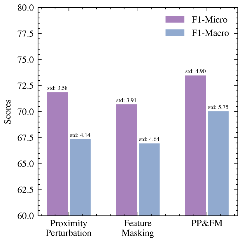
(a) PROTEINS_full

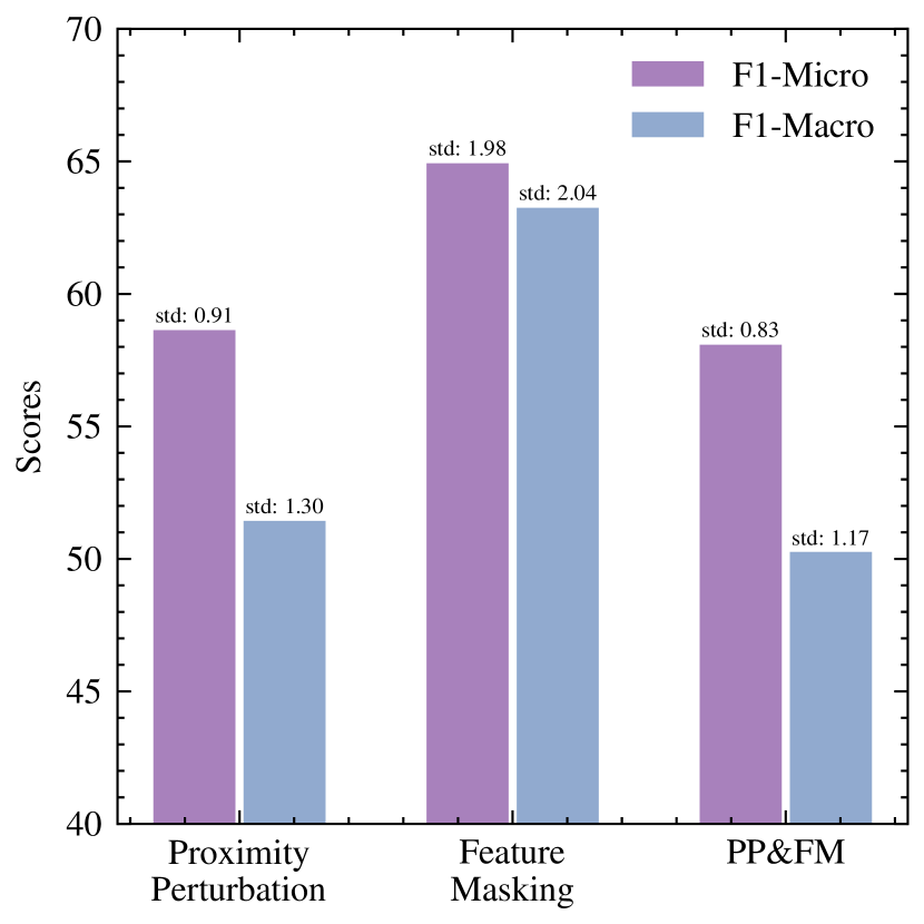
(b) FRANKENSTEIN

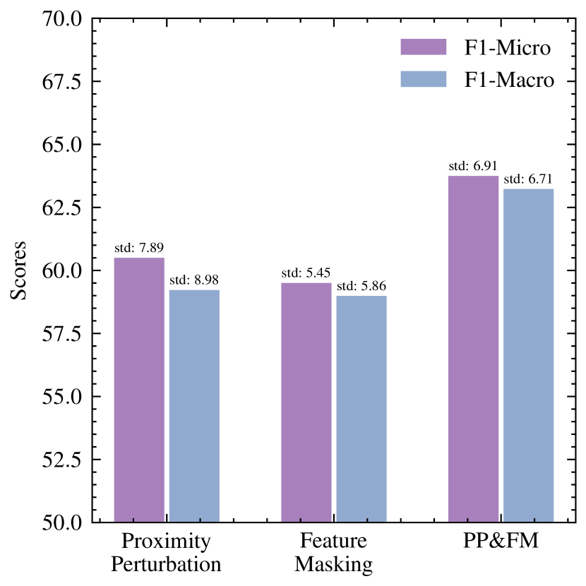
(c) Synthie

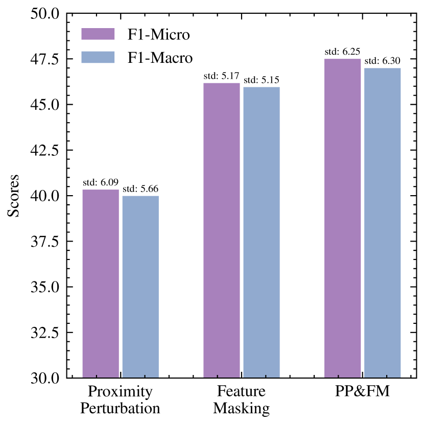
(d) ENZYMES

Figure 4. Graph classification results of the proposed method with different hard negative samples.

Graph classification results of the proposed method with different hard negative samples.

For reproducibility, we introduce the detailed settings of the proposed method. For PROTEINS_full, FRANKENSTEIN, and Synthie, we take GCN (Kipf and Welling, 2017) with three layers as the graph encoder. The learning rates for hard negative sample generation and contrastive learning are 0.0001. The training epochs for the two training stages are 80 and 30, respectively. For dataset ENZYMES, we adopt a 2-layer GIN (Xu et al., 2019) as the graph encoder. The learning rates for hard negative sample generation and contrastive learning are 0.001. The training epochs for both training stages are 100. The batch sizes for all the experiments are set to 256, while 128 is also feasible if GPU memory is limited for large graphs such as Synthie. The threshold $\omega$ and $\gamma$ mentioned previously are both 0.3. As to the temperature hyperparameter for contrastive learning, it is set to 1 for all the experiments. We evaluate the proposed method via graph classification under the linear evaluation protocol. Specifically, we closely follow the evaluation protocol in InfoGraph and report the mean 10-fold cross-validation F1-Micro and F1-macro scores with standard deviation output by a linear SVM.

4.4. Comparison Experiment

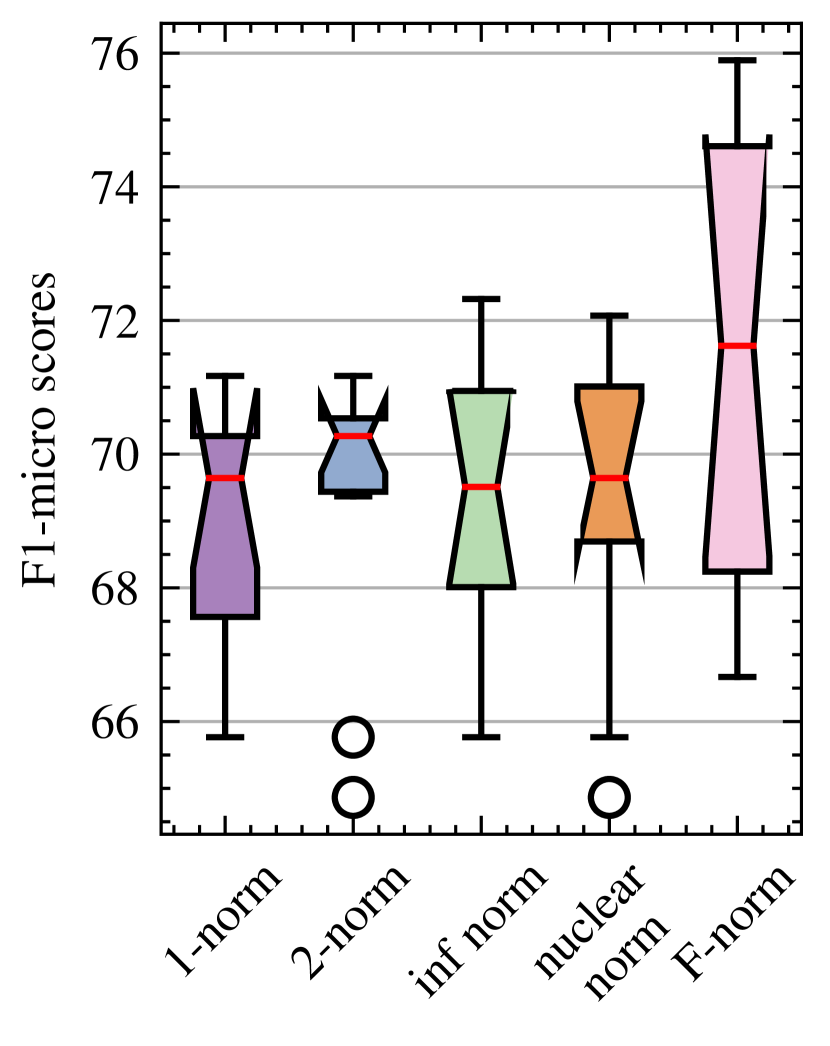
(a) F1-Micro, PROTEINS_full

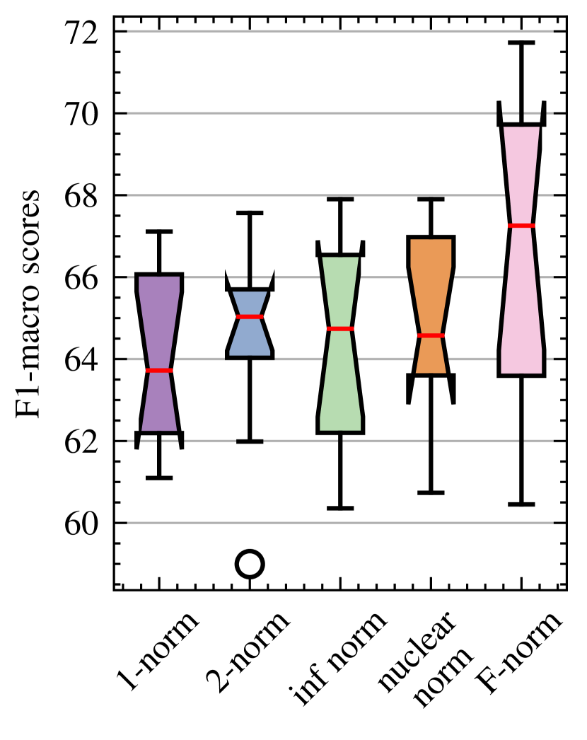
(b) F1-Macro, PROTEINS_full

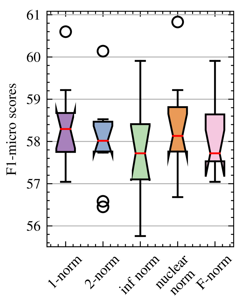
(c) F1-Micro, FRANKENSTEIN

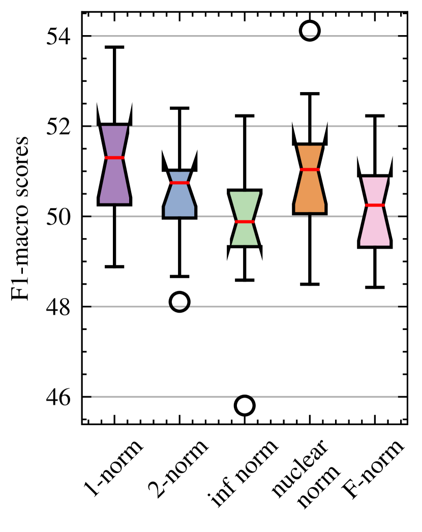
(d) F1-Macro, FRANKENSTEIN

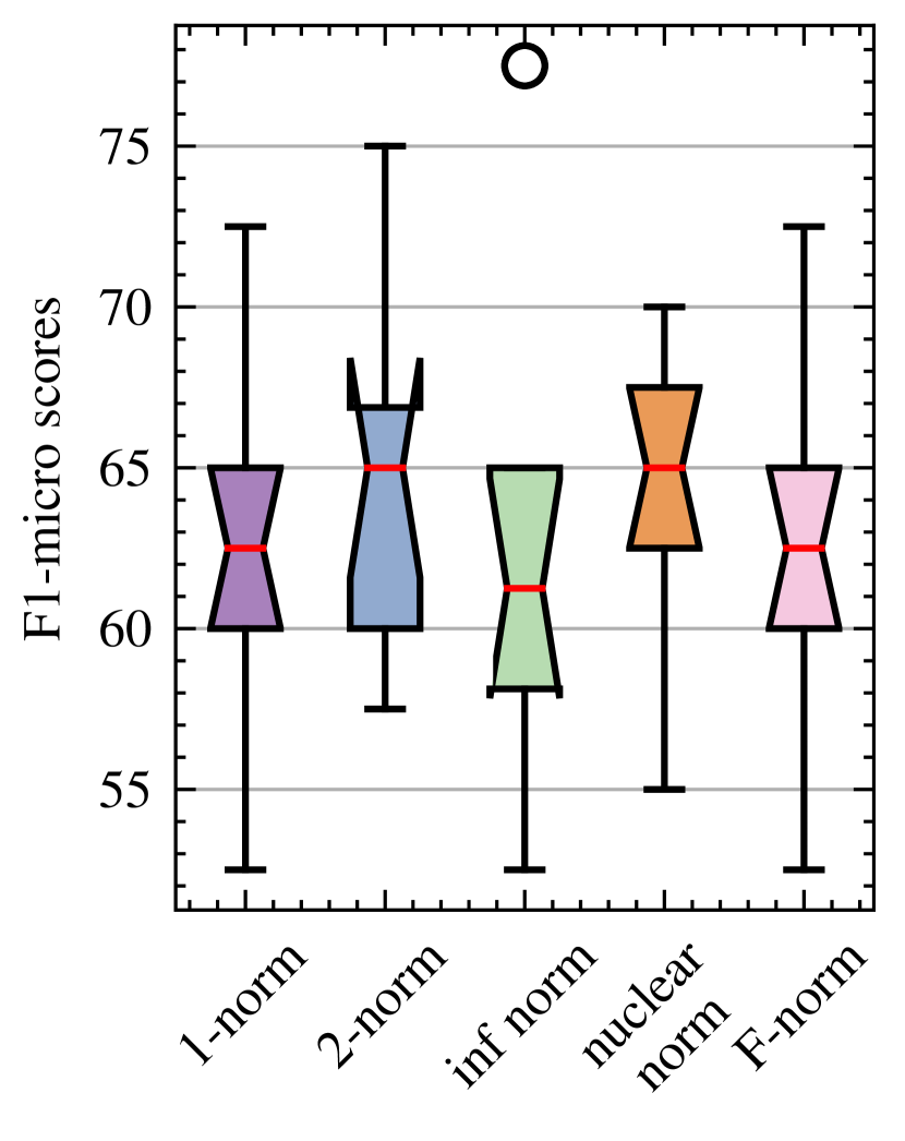
(e) F1-Micro, Synthie

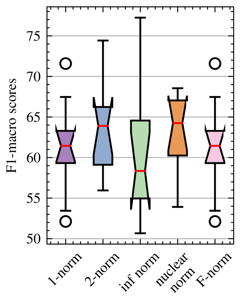
(f) F1-Macro, Synthie

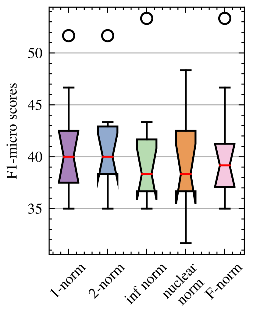
(g) F1-Micro, ENZYMES

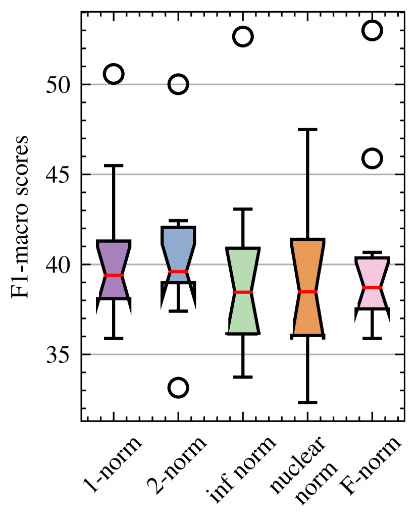
(h) F1-Macro, ENZYMES

Figure 5. The performances of the proposed method on all the datasets with hard negative samples, whose generation procedure adopts different matrix norms to measure similarity between the original input and the generated graphs.

The performances of the proposed method on all the datasets with hard negative samples, whose generation procedure adopts different matrix norms to measure similarity between the original input and the generated graphs.

The comparison experiment results for all baselines and our proposed method on all four datasets are shown in Table 2. Generally, the proposed method outperforms the best baselines on all the datasets except PROTEINS_full. Though our method has a mean F1-macro score lower than that of GraphCL, the gap between its F1-macro score and ours is insignificant as the standard deviation exists. We note that the proposed method significantly improves the dataset Synthie and ENZYMES. According to Table 1, both of these datasets have multiple classes, which are 4 and 6, respectively. It indicates that the proposed method is superior in multiclass graph classification tasks. Recall one of the training objectives of hard negative samples generation, Equation (9), which minimises the similarity between the probability distributions of which class the original graph and hard negative samples are. If there were a multiclass classification task, the Equation (9) would minimise the similarity between two vectors (the vector refers to the probability distribution in our context) with more dimensions. Comparing two vectors with higher dimensionality could help the model to learn more information. So, it is reasonable that the proposed method has advantages on dataset Synthie and ENZYMES.

Graph kernel methods also achieve good performances compared to novel neural network methods. Nevertheless, some of them spend time on computing. Compared to our proposed method, they cannot be accelerated by GPUs, which is unaffordable under some real-world scenarios. Sub2Vec and Graph2Vec are two impactful graph embedding methods, which both leverage the idea of Word2Vec (Mikolov et al., 2013). According to the experiment results, they cannot compete with the graph contrastive learning method, which is a novel and effective unsupervised graph learning paradigm nowadays.

Note that we selected four graph contrastive learning methods as baselines. All of them are impactful methods in the graph contrastive learning domain. InfoGraph is one of the first methods to introduce the idea of contrastive learning into the graph representation learning area. It achieved promising performances on several graph learning tasks. As shown in Table 2, it has satisfying results on dataset PROTEINS_full and FRANKENSTEIN. However, it may not be compatible with multiclass graph classification tasks, as the proposed CGC significantly outperforms it. Conversely, MVGRL performs better on Synthie and ENZYMES than on the other two datasets with only two classes. GCA is an updated version of GraphCL, and they share the same framework, but the improvement achieved by GCA is not significant. It has minor improvement on the dataset FRANKENSTEIN and ENZYMES. On dataset Synthie, it even has much worse performances. GraphCL and GCA try to conduct proper perturbations on the target to have positive or negative samples to form contrasting pairs. Specifically, GraphCL follows a random setting to perturb the graph, which cannot ensure the quality of the generated samples. GCA tries to adaptively locate the essential elements in the graph and perturb such identified elements according to their centrality. However, elements with high centrality are not always the critical factor determining the labels or semantics of the graph. Compared to our counterfactual hard negative samples generation method, these two methods have limitations in contrasting pairs generation. We also note that GraphCL and GCA are incompatible with multiclass graph classification tasks. This is because the implementations of GraphCL and GCA both take the implementation of InfoGraph as the backbone. It is reasonable for them to have such a phenomenon.

4.5. Ablation Study

4.5.1. The impact on the graph contrastive learning with different types of generated hard negative samples.

Recall that we proposed to generate two different types of hard negative samples. In this section, we want to find out how much improvement can be brought by different hard negative samples. We conducted several experiments on the proposed method. We proceed with the graph contrastive learning procedure under three scenarios, which are 1) only to use the proximity perturbed graphs as a negative sample, 2) only to use the feature-masked graphs as negative samples, and 3) utilizing both types of graphs as negative samples. The results of the experiments are illustrated in Figure 4(d). Utilizing both types of negative samples can achieve the best performances on all the datasets except FRANKENSTEIN. To achieve better results, utilising two hard negative samples can help the model capture the key semantics in proximity and feature space simultaneously. Moreover, we can form more contrasting pairs with more negative samples. Hence, the model can receive sufficient self-supervised signals to update parameters and perform better.

On dataset FRANKENSTEIN, the experiment results are not what we expected. The model trained only with the feature-masked graphs achieved the best performance. There is a significant gap between the performance of the model trained only with the proximity perturbed graphs and the model trained only with the feature-masked graphs. Such a gap makes the collaboration of two types of negative samples unsatisfying, resulting in the worse performance of the model trained with both types of generated negative samples. Though the gap between the mean F1 scores of the model trained only with the proximity perturbed graphs and the model trained only with the feature-masked graphs on dataset ENZYMES is also significant, we note there is a larger standard deviation in the experimental results on the dataset ENZYMES. In this case, such a phenomenon indicates that the differences between the performances of the model trained only with the proximity perturbed graphs and the model trained only with the feature-masked graphs on dataset ENZYMES are not as significant as that on dataset FRANKENSTEIN. According to Table 1, graphs in dataset FRANKENSTEIN have much fewer nodes and edges than the other three datasets, but they have significantly larger node feature dimensionality. Masking features can bring more advantages to the model on dataset FRANKENSTEIN since the feature matrices are more complicated than the adjacency matrices. Such imbalance results in a considerable gap between the performances of the model trained only with the proximity perturbed graphs and the model trained only with the feature-masked graphs on dataset FRANKENSTEIN. We claim that perturbation to the aspects containing more informative semantics would bring more advantages to graph contrastive learning. Similar phenomena appear in the rest datasets. For example, graphs in dataset PROTEINS_full and Synthie have complicated adjacency matrices with simple feature matrices. On these two datasets, the model trained only with the feature-masked graphs outperforms the model trained only with the proximity perturbed graphs.

4.5.2. How to measure the similarity in hard negative samples generation procedure?

Table 3. Five types of matrix norms and their definitions, where $M^{*}$ denotes the conjugate transpose of matrix $M\in\mathbb{R}^{n\times m}$, $\lambda_{max}(\cdot)$ is the function to have the largest eigenvalue of some matrix, and $tr(\cdot)$ represents trace function.

Matrix Norm	Definition	Complexity
1-norm	$||M||_{1}=\max_{1\leq j\leq n}\sum^{m}_{i=1}|m_{ij}|$	$\mathcal{O}(mn)$
2-norm	$||M||_{2}=\sqrt{\lambda_{max}(M^{*}M)}$	$\mathcal{O}(m^{3})$
inf norm	$||M||_{\infty}=\max_{1\leq i\leq m}\sum^{n}_{j=1}|m_{ij}|$	$\mathcal{O}(mn)$
nuclear norm	$||M||_{*}=tr(\sqrt{M^{T}M})$	$\mathcal{O}(mn^{2})$
F-norm	$||M||_{F}=\sqrt{\sum_{i=1}^{m}\sum_{j=1}^{n}|m_{ij}|^{2}}$	$\mathcal{O}(mn)$

Ensuring the generated negative samples have similar forms to the original input in proximity and feature space is the key to making the negative samples be hard. A proper similarity measurement is important to achieve such a goal. In the methodology section, we introduced that we measure the similarity between the original input and the generated negative samples via calculating the norms of difference matrices $||A-A^{\prime}_{a}||$ and $M^{\prime}_{b}$. However, there are many different matrix norms. In this section, we examine the performances of the model trained with the negative samples in which different matrix norms were applied. We consider five different matrix norms shown in Table 3, and the experimental results are illustrated in Figure 5(h).

Following the proposed generation protocol, the cost of 2-norm and nuclear norm is much larger than others due to their computation complexity. Therefore, using these two matrix norms is not practical. As to inf norm, its performances vary among all the datasets. The performances are not stable. Hence, 1-norm and F-norm are more suitable for the similarity measurement in our hard negative samples generation protocol. Considering the simplicity of 1-norm, in most cases, it is a better option since it can achieve equivalent performances compared to F-norm.

5. Conclusion

In this paper, we proposed a novel method, named CGC, to generate hard negative samples for graph contrastive learning. Compared to current graph contrastive learning methods and some classical graph kernel and graph embedding methods, it achieved state-of-the-art performances in most cases. We studied the effectiveness of the model trained with different types of generated hard negative samples. We found that perturbation made on the more complicated part of the graph data (e.g., node features or proximity) would bring more advantages to graph contrastive learning. Furthermore, we explore how to choose similarity measurement for hard negative sample generation from a perspective of matrix norm. There will be more methods to conduct such a task, and it would be interesting future work to improve the proposed method in this paper.

- (1)
- Adhikari et al. (2018) Bijaya Adhikari, Yao Zhang, Naren Ramakrishnan, and B. Aditya Prakash. 2018. Sub2Vec: Feature Learning for Subgraphs. In Advances in Knowledge Discovery and Data Mining - 22nd Pacific-Asia Conference, PAKDD 2018, Melbourne, VIC, Australia, June 3-6, 2018, Proceedings, Part II (Lecture Notes in Computer Science), Dinh Q. Phung, Vincent S. Tseng, Geoffrey I. Webb, Bao Ho, Mohadeseh Ganji, and Lida Rashidi (Eds.), Vol. 10938. Springer, 170–182. https://doi.org/10.1007/978-3-319-93037-4_14
- Borgwardt and Kriegel (2005) Karsten M. Borgwardt and Hans-Peter Kriegel. 2005. Shortest-Path Kernels on Graphs. In Proceedings of the 5th IEEE International Conference on Data Mining (ICDM 2005), 27-30 November 2005, Houston, Texas, USA. IEEE Computer Society, 74–81. https://doi.org/10.1109/ICDM.2005.132
- Borgwardt et al. (2005) Karsten M. Borgwardt, Cheng Soon Ong, Stefan Schönauer, S. V. N. Vishwanathan, Alexander J. Smola, and Hans-Peter Kriegel. 2005. Protein function prediction via graph kernels. In Proceedings Thirteenth International Conference on Intelligent Systems for Molecular Biology 2005, Detroit, MI, USA, 25-29 June 2005. 47–56. https://doi.org/10.1093/bioinformatics/bti1007
- Clark et al. (2020) Kevin Clark, Minh-Thang Luong, Quoc V. Le, and Christopher D. Manning. 2020. ELECTRA: Pre-training Text Encoders as Discriminators Rather Than Generators. In 8th International Conference on Learning Representations, ICLR 2020, Addis Ababa, Ethiopia, April 26-30, 2020. OpenReview.net. https://openreview.net/forum?id=r1xMH1BtvB
- Fan et al. (2022) Wenqi Fan, Xiaorui Liu, Wei Jin, Xiangyu Zhao, Jiliang Tang, and Qing Li. 2022. Graph trend filtering networks for recommendation. In Proceedings of the 45th International ACM SIGIR Conference on Research and Development in Information Retrieval. 112–121.
- Hassani and Ahmadi (2020) Kaveh Hassani and Amir Hosein Khas Ahmadi. 2020. Contrastive Multi-View Representation Learning on Graphs. In Proceedings of the 37th International Conference on Machine Learning, ICML 2020, 13-18 July 2020, Virtual Event (Proceedings of Machine Learning Research), Vol. 119. PMLR, 4116–4126. http://proceedings.mlr.press/v119/hassani20a.html
- He et al. (2020) Kaiming He, Haoqi Fan, Yuxin Wu, Saining Xie, and Ross B. Girshick. 2020. Momentum Contrast for Unsupervised Visual Representation Learning. In 2020 IEEE/CVF Conference on Computer Vision and Pattern Recognition, CVPR 2020, Seattle, WA, USA, June 13-19, 2020. Computer Vision Foundation / IEEE, 9726–9735. https://doi.org/10.1109/CVPR42600.2020.00975
- Jin et al. (2022) Wei Jin, Xiaorui Liu, Xiangyu Zhao, Yao Ma, Neil Shah, and Jiliang Tang. 2022. Automated Self-Supervised Learning for Graphs. In 10th International Conference on Learning Representations (ICLR 2022).
- Kipf and Welling (2017) Thomas N. Kipf and Max Welling. 2017. Semi-Supervised Classification with Graph Convolutional Networks. In 5th International Conference on Learning Representations, ICLR 2017, Toulon, France, April 24-26, 2017, Conference Track Proceedings. OpenReview.net. https://openreview.net/forum?id=SJU4ayYgl
- Kullback and Leibler (1951) S. Kullback and R. A. Leibler. 1951. On Information and Sufficiency. The Annals of Mathematical Statistics 22, 1 (1951), 79 – 86. https://doi.org/10.1214/aoms/1177729694
- Li et al. (2022) Xiao-Hui Li, Caleb Chen Cao, Yuhan Shi, Wei Bai, Han Gao, Luyu Qiu, Cong Wang, Yuanyuan Gao, Shenjia Zhang, Xun Xue, and Lei Chen. 2022. A Survey of Data-Driven and Knowledge-Aware eXplainable AI. IEEE Trans. Knowl. Data Eng. 34, 1 (2022), 29–49. https://doi.org/10.1109/TKDE.2020.2983930
- Mikolov et al. (2013) Tomás Mikolov, Kai Chen, Greg Corrado, and Jeffrey Dean. 2013. Efficient Estimation of Word Representations in Vector Space. In 1st International Conference on Learning Representations, ICLR 2013, Scottsdale, Arizona, USA, May 2-4, 2013, Workshop Track Proceedings, Yoshua Bengio and Yann LeCun (Eds.). http://arxiv.org/abs/1301.3781
- Morris et al. (2020) Christopher Morris, Nils M. Kriege, Franka Bause, Kristian Kersting, Petra Mutzel, and Marion Neumann. 2020. TUDataset: A collection of benchmark datasets for learning with graphs. CoRR abs/2007.08663 (2020). arXiv:2007.08663 https://arxiv.org/abs/2007.08663
- Morris et al. (2016) Christopher Morris, Nils M. Kriege, Kristian Kersting, and Petra Mutzel. 2016. Faster Kernels for Graphs with Continuous Attributes via Hashing. In IEEE 16th International Conference on Data Mining, ICDM 2016, December 12-15, 2016, Barcelona, Spain, Francesco Bonchi, Josep Domingo-Ferrer, Ricardo Baeza-Yates, Zhi-Hua Zhou, and Xindong Wu (Eds.). IEEE Computer Society, 1095–1100. https://doi.org/10.1109/ICDM.2016.0142
- Narayanan et al. (2017) Annamalai Narayanan, Mahinthan Chandramohan, Rajasekar Venkatesan, Lihui Chen, Yang Liu, and Shantanu Jaiswal. 2017. graph2vec: Learning Distributed Representations of Graphs. CoRR abs/1707.05005 (2017). arXiv:1707.05005 http://arxiv.org/abs/1707.05005
- Orsini et al. (2015) Francesco Orsini, Paolo Frasconi, and Luc De Raedt. 2015. Graph Invariant Kernels. In Proceedings of the Twenty-Fourth International Joint Conference on Artificial Intelligence, IJCAI 2015, Buenos Aires, Argentina, July 25-31, 2015, Qiang Yang and Michael J. Wooldridge (Eds.). AAAI Press, 3756–3762. http://ijcai.org/Abstract/15/528
- Pearl and Mackenzie (2018) Judea Pearl and Dana Mackenzie. 2018. The Book of Why: The New Science of Cause and Effect (1st ed.). Basic Books, Inc., USA.
- Qiu et al. (2020) Jiezhong Qiu, Qibin Chen, Yuxiao Dong, Jing Zhang, Hongxia Yang, Ming Ding, Kuansan Wang, and Jie Tang. 2020. GCC: Graph Contrastive Coding for Graph Neural Network Pre-Training. In KDD ’20: The 26th ACM SIGKDD Conference on Knowledge Discovery and Data Mining, Virtual Event, CA, USA, August 23-27, 2020. ACM, 1150–1160. https://doi.org/10.1145/3394486.3403168
- Robinson et al. (2021) Joshua David Robinson, Ching-Yao Chuang, Suvrit Sra, and Stefanie Jegelka. 2021. Contrastive Learning with Hard Negative Samples. In 9th International Conference on Learning Representations, ICLR 2021, Virtual Event, Austria, May 3-7, 2021. OpenReview.net. https://openreview.net/forum?id=CR1XOQ0UTh-
- Schomburg et al. (2004) Ida Schomburg, Antje Chang, Christian Ebeling, Marion Gremse, Christian Heldt, Gregor Huhn, and Dietmar Schomburg. 2004. BRENDA, the enzyme database: updates and major new developments. Nucleic Acids Res. 32, Database-Issue (2004), 431–433. https://doi.org/10.1093/nar/gkh081
- Shervashidze et al. (2011) Nino Shervashidze, Pascal Schweitzer, Erik Jan van Leeuwen, Kurt Mehlhorn, and Karsten M. Borgwardt. 2011. Weisfeiler-Lehman Graph Kernels. J. Mach. Learn. Res. 12 (2011), 2539–2561. http://dl.acm.org/citation.cfm?id=2078187
- Shervashidze et al. (2009) Nino Shervashidze, S. V. N. Vishwanathan, Tobias Petri, Kurt Mehlhorn, and Karsten M. Borgwardt. 2009. Efficient graphlet kernels for large graph comparison. In Proceedings of the Twelfth International Conference on Artificial Intelligence and Statistics, AISTATS 2009, Clearwater Beach, Florida, USA, April 16-18, 2009 (JMLR Proceedings), David A. Van Dyk and Max Welling (Eds.), Vol. 5. JMLR.org, 488–495. http://proceedings.mlr.press/v5/shervashidze09a.html
- Sun et al. (2020) Fan-Yun Sun, Jordan Hoffmann, Vikas Verma, and Jian Tang. 2020. InfoGraph: Unsupervised and Semi-supervised Graph-Level Representation Learning via Mutual Information Maximization. In 8th International Conference on Learning Representations, ICLR 2020, Addis Ababa, Ethiopia, April 26-30, 2020. OpenReview.net. https://openreview.net/forum?id=r1lfF2NYvH
- van den Oord et al. (2018) Aäron van den Oord, Yazhe Li, and Oriol Vinyals. 2018. Representation Learning with Contrastive Predictive Coding. CoRR abs/1807.03748 (2018). arXiv:1807.03748 http://arxiv.org/abs/1807.03748
- Velickovic et al. (2019) Petar Velickovic, William Fedus, William L. Hamilton, Pietro Liò, Yoshua Bengio, and R. Devon Hjelm. 2019. Deep Graph Infomax. In 7th International Conference on Learning Representations, ICLR 2019, New Orleans, LA, USA, May 6-9, 2019. OpenReview.net. https://openreview.net/forum?id=rklz9iAcKQ
- Vishwanathan et al. (2010) S. V. N. Vishwanathan, Nicol N. Schraudolph, Risi Kondor, and Karsten M. Borgwardt. 2010. Graph Kernels. J. Mach. Learn. Res. 11 (2010), 1201–1242. http://portal.acm.org/citation.cfm?id=1859891
- Wachter et al. (2018) S Wachter, BDM Mittelstadt, and C Russell. 2018. Counterfactual explanations without opening the black box: automated decisions and the GDPR. Harvard Journal of Law and Technology 31, 2 (2018), 841–887.
- Wang et al. (2021) Cong Wang, Xiao-Hui Li, Haocheng Han, Shendi Wang, Luning Wang, Caleb Chen Cao, and Lei Chen. 2021. Counterfactual Explanations in Explainable AI: A Tutorial. In KDD ’21: The 27th ACM SIGKDD Conference on Knowledge Discovery and Data Mining, Virtual Event, Singapore, August 14-18, 2021, Feida Zhu, Beng Chin Ooi, and Chunyan Miao (Eds.). ACM, 4080–4081. https://doi.org/10.1145/3447548.3470797
- Wu et al. (2018) Zhirong Wu, Yuanjun Xiong, Stella X. Yu, and Dahua Lin. 2018. Unsupervised Feature Learning via Non-Parametric Instance Discrimination. In 2018 IEEE Conference on Computer Vision and Pattern Recognition, CVPR 2018, Salt Lake City, UT, USA, June 18-22, 2018. Computer Vision Foundation / IEEE Computer Society, 3733–3742. https://doi.org/10.1109/CVPR.2018.00393
- Xia et al. (2021) Jun Xia, Lirong Wu, Jintao Chen, Ge Wang, and Stan Z. Li. 2021. Debiased Graph Contrastive Learning. CoRR abs/2110.02027 (2021). arXiv:2110.02027 https://arxiv.org/abs/2110.02027
- Xu et al. (2019) Keyulu Xu, Weihua Hu, Jure Leskovec, and Stefanie Jegelka. 2019. How Powerful are Graph Neural Networks?. In 7th International Conference on Learning Representations, ICLR 2019, New Orleans, LA, USA, May 6-9, 2019. OpenReview.net. https://openreview.net/forum?id=ryGs6iA5Km
- Yang et al. (2022) Haoran Yang, Hongxu Chen, Shirui Pan, Lin Li, Philip S. Yu, and Guandong Xu. 2022. Dual Space Graph Contrastive Learning. CoRR abs/2201.07409 (2022). arXiv:2201.07409 https://arxiv.org/abs/2201.07409
- You et al. (2020) Yuning You, Tianlong Chen, Yongduo Sui, Ting Chen, Zhangyang Wang, and Yang Shen. 2020. Graph Contrastive Learning with Augmentations. In Advances in Neural Information Processing Systems 33: Annual Conference on Neural Information Processing Systems 2020, NeurIPS 2020, December 6-12, 2020, virtual. https://proceedings.neurips.cc/paper/2020/hash/3fe230348e9a12c13120749e3f9fa4cd-Abstract.html
- Zhao et al. (2021) Han Zhao, Xu Yang, Zhenru Wang, Erkun Yang, and Cheng Deng. 2021. Graph Debiased Contrastive Learning with Joint Representation Clustering. In Proceedings of the Thirtieth International Joint Conference on Artificial Intelligence, IJCAI 2021, Virtual Event / Montreal, Canada, 19-27 August 2021, Zhi-Hua Zhou (Ed.). ijcai.org, 3434–3440. https://doi.org/10.24963/ijcai.2021/473
- Zhu et al. (2021) Yanqiao Zhu, Yichen Xu, Feng Yu, Qiang Liu, Shu Wu, and Liang Wang. 2021. Graph Contrastive Learning with Adaptive Augmentation. In WWW ’21: The Web Conference 2021, Virtual Event / Ljubljana, Slovenia, April 19-23, 2021. ACM / IW3C2, 2069–2080. https://doi.org/10.1145/3442381.3449802