More constraints on the Georgi-Machacek model

Abstract

In this work, we investigate the parameter space of the Georgi-Machacek (GM) model, where we consider many theoretical and experimental constraints such as the perturbativity, vacuum stability, unitarity, electroweak precision tests, the Higgs diphoton decay, the Higgs total decay width and the LHC measurements of the signal strengths of the SM-like Higgs boson $h$ in addition to the constraints from doubly charged Higgs bosons and Drell-Yan diphoton production and the indirect constraint from the $b\to s$ transition processes. We investigate also the possibility that the electroweak vacuum could be destabilized by unwanted wrong minima that may violate the $CP$ and/or the electric charge symmetries. We found that about 40 % of the parameter space that fulfills the above mentioned constraints are excluded by these unwanted minima. In addition, we found that the negative searches for a heavy resonance could exclude a significant part of the viable parameter space, and future searches could exclude more regions in the parameter space.

I Introduction

Since the discovery of a Standard Model (SM)-like 125 GeV Higgs boson at the Large Hadron Collider (LHC) ATLAS:2012yve , many questions are still open, where the SM provides no answers. For instance, the Higgs mass is found to be at the electroweak (EW) scale, while it may acquire very large radiative corrections that can reach the Planck or GUT scales within the SM. This hierarchy problem requires an unwanted fine-tuning. In addition, there are unanswered questions such as the fermions masses of difference, the origin of $CP$ violation in the quark sector, the dark matter nature Bertone:2004pz and the neutrino oscillation data Super-Kamiokande:1998kpq .

The discovered 125 GeV scalar has the properties of a SM-like Higgs; however, it is not known yet whether the electroweak symmetry breaking (EWSB) is triggered by one single scalar field or more. In many SM extensions, the EWSB is achieved via more than one scalar where many scalar fields acquire nonvanishing vacuum expectation values (VEVs), and the SM-like is a composite. Among these SM extensions, the so-called Georgi-Machacek (GM) model Georgi:1985nv , where the ESWB is realized by three scalar fields. In addition to the SM doublet, the GM model includes one complex and one real scalar triplets, where a global custodial $SU(2)_{V}$ symmetry is preserved in the scalar potential after the EWSB. The scalar vacuum in the GM model is defined in a way that the $\rho$-parameter should be within the experimentally allowed range Workman:2022ynf ,

$$\rho=\frac{g_{hWW}^{SM}}{g_{hZZ}^{SM}\cos^{2}\theta_{w}}=1.00039\pm 0.00019,$$ (1)

with $g_{hWW}^{SM}=2m_{W}^{2}/\upsilon$ and $g_{hZZ}^{SM}=2m_{Z}^{2}/\upsilon$, where $\upsilon=246.22\,\textrm{GeV}$. This leads to a scalar spectrum with different multiplets under the global $SU(2)_{V}$ custodial symmetry, whose mass eigenstates give a quintet ($H_{5}$), a triplet ($H_{3}$) and two $CP-even$ singlets ($\eta$ and $h$). In our work, we consider the parameter space that corresponds to $h=h_{125}$, with $m_{\eta}>m_{h}$. One has to mention that an interesting viable parameter space exists for the case $m_{\eta}<m_{h}$, where interesting collider signatures are possible Ahriche:2022aoj .

Due to the feature that the SM-like Higgs couplings to both $W$ and $Z$ gauge bosons could be significantly different than the SM values Chiang:2013rua , the GM model could be phenomenologically interesting. In addition to the existence of additional $CP-odd$, singly and doubly charged scalars, the GM model could be a good benchmark for searches of beyond SM scalars; which has been extensively investigated in the literature Chanowitz:1985ug . In the decoupling limit Hartling:2014zca , all additional beyond SM particles that are present in the GM model become heavy and the fermion and gauge bosons couplings to the SM-like Higgs boson approach the SM values. In addition to the rich phenomenology, other issues were addressed within the GM model such as the neutrino mass Chen:2020ark , dark matter Pilkington:2017qam , and the electroweak phase transition strength Chiang:2014hia .

Recent measurements and negative searches at the LHC Workman:2022ynf , such as those of the total decay width, Higgs strength modifiers and the cross section upper bounds from negative searches of new scalar resonance, could imply significant constraints on the GM model parameter space. Although the GM model includes a custodial scalar fiveplet, it has been shown that the LHC searches for the doubly charged Higgs bosons in the VBF channel $H_{5}^{++}\to W^{+}W^{+}$ and the Drell-Yan production of a neutral Higgs boson $pp\to H_{5}^{0}(\gamma\gamma)H^{+}$ impose interesting bounds on the parameter space Ismail:2020zoz , as well as the indirect constraints from the $b\to s$ transition processes that exclude all the benchmark points (BPs) with large $\upsilon_{\xi}$ Hartling:2014aga . In addition, the GM scalar potential structure may admit many minima beside the electroweak (EW) vacuum that could break the electric charge and/or the $CP$ symmetry spontaneously. In case where such minima exist, they should not be deeper than the EW vacuum, which may affect the parameter space that is in agreement with the previously mentioned constraints. In Chiang:2018cgb , the authors performed a global fit analysis for the GM model free parameter and obtained some limits on the mixing angles and the heavy new scalar masses and decay widths. However, since the constraints from the $b\to s$ transition processes were considered in Chiang:2018cgb ; and the LHC measurements used to constrain the GM model have been significantly updated, an analysis for the full model parameter space is required. Here, we aim to investigate the impact of all the relevant constraints on the model by performing a full numerical scan over the whole parameter space.

In this work, we give a brief introduction of the GM model in Sec II, where the scalar potential and the mass spectrum are described. In Sec III, we discuss the possible existence of new minima that could be deeper than the EW vacuum. Then, after categorizing these unwanted minima according to the preserved/broken ($CP$ and electric charge) symmetries, one considers the EW vacuum to be the deepest one as an novel constraint on the GM model. In Sec IV, we discuss different theoretical and experimental constraints on the model such as the unitarity, vacuum stability, the total Higgs decay width and signal strength modifiers, the electroweak precision tests, and the diphoton Higgs decay. In addition, we consider the recent ATLAS and CMS constraints on the heavy $CP-even$ scalar $\eta$ and from the negative searches for the doubly charged Higgs bosons in the VBF channel $H_{5}^{++}\to W^{+}W^{+}$, and the Drell-Yan production of a neutral Higgs boson $pp\to H_{5}^{0}(\gamma\gamma)H^{+}$. We show our numerical results and discussion in Sec V, and our conclusion in Sec VI.

II The Model: Parameters and Mass Spectrum

In the GM model, the scalar sector consists of a scalar doublet $(\phi^{+},\,\phi^{0})^{T}$ with hypercharge $Y=1$, and two triplet representations $(\chi^{++},\,\chi^{+},\,\chi^{0})^{T}$ and $(\xi^{+},\,\xi^{0},\,-\xi^{-})^{T}$ with hypercharge $Y=2,0$, respectively. These representations can be written as

$$\Phi=\left(\begin{array}[]{cc}\phi^{0*}&\phi^{+}\\ -\phi^{+*}&\phi^{0}\end{array}\right),\quad\Delta=\left(\begin{array}[]{ccc}\chi^{0*}&\xi^{+}&\chi^{++}\\ -\chi^{+*}&\xi^{0}&\chi^{+}\\ \chi^{++*}&-\xi^{+*}&\chi^{0}\end{array}\right),$$ (2)

where $\phi^{-}=\phi^{+*},\,\xi^{-}=\xi^{+*},\,\chi^{--}=\chi^{++*},\,\chi^{-}=\chi^{+*}.$ The neutral components in (2) can be expressed by

$$\phi^{0}=\frac{1}{\sqrt{2}}(\upsilon_{\phi}+h_{\phi}+ia_{\phi}),\,\chi^{0}=\frac{1}{\sqrt{2}}(\upsilon_{\chi}+h_{\chi}+ia_{\chi}),\,\xi^{0}=\upsilon_{\xi}+h_{\xi},$$ (3)

where $\upsilon_{\phi},\,\upsilon_{\chi}$ and $\upsilon_{\xi}$ are the VEVs for $\phi^{0},\,\chi^{0}$ and $\xi^{0}$, respectively. Here, we have three $CP-even$ scalar degrees of freedom (d.o.f.) $\{h_{\phi},\,h_{\chi},\,h_{\xi}\}$, two $CP-odd$ d.o.f. $\{a_{\phi},\,a_{\chi}\}$, six singly charged d.o.f. $\{\phi^{\pm},\chi^{\pm},\xi^{\pm}\}$ and two doubly charged d.o.f. $\chi^{\pm\pm}$. The most general scalar potential invariant under the global symmetry $SU(2)_{L}\times SU(2)_{R}\times U(1)_{Y}$ is given by

$$V(\varPhi,\Delta) =\frac{m_{1}^{2}}{2}\mathrm{Tr}[\varPhi^{\dagger}\varPhi]+\frac{m_{2}^{2}}{2}\mathrm{Tr}[\Delta^{\dagger}\Delta]+\lambda_{1}(\mathrm{Tr}[\varPhi^{\dagger}\varPhi])^{2}+\lambda_{2}\mathrm{Tr}[\varPhi^{\dagger}\varPhi]\mathrm{Tr}[\Delta^{\dagger}\Delta]$$

$$+\lambda_{3}\mathrm{Tr}[(\Delta^{\dagger}\Delta)^{2}]+\lambda_{4}(\mathrm{Tr}[\Delta^{\dagger}\Delta])^{2}-\lambda_{5}\mathrm{Tr}[\varPhi^{\dagger}\frac{\sigma^{a}}{2}\varPhi\frac{\sigma^{b}}{2}]\mathrm{Tr}[\Delta^{\dagger}T^{a}\Delta T^{b}]$$

$$-\mu_{1}\mathrm{Tr}[\varPhi^{\dagger}\frac{\sigma^{a}}{2}\varPhi\frac{\sigma^{b}}{2}](U\Delta U^{\dagger})_{ab}-\mu_{2}\mathrm{Tr}[\Delta^{\dagger}T^{a}\Delta T^{b}](U\Delta U^{\dagger})_{ab},$$ (4)

with $\sigma^{1,2,3}$ are the Pauli matrices and $T^{1,2,3}$ correspond to the generators of the $SU(2)$ triplet representation, that are given by

$$T^{1}=\frac{1}{\sqrt{2}}\left(\begin{array}[]{ccc}0&1&0\\ 1&0&1\\ 0&1&0\end{array}\right),\>T^{2}=\frac{1}{\sqrt{2}}\left(\begin{array}[]{ccc}0&-i&0\\ i&0&-i\\ 0&i&0\end{array}\right),\,T^{3}=\left(\begin{array}[]{ccc}1&0&0\\ 0&0&0\\ 0&0&-1\end{array}\right),$$ (5)

and the matrix $U$ is defined as

$$U=\frac{1}{\sqrt{2}}\left(\begin{array}[]{ccc}-1&0&1\\ -i&0&-i\\ 0&\sqrt{2}&0\end{array}\right).$$ (6)

The custodial symmetry condition at tree-level $m_{W}^{2}=m_{Z}^{2}\cos^{2}\theta_{W}$ implies $\upsilon_{\chi}=\sqrt{2}\upsilon_{\xi}$ and $\upsilon_{\phi}^{2}+8\upsilon_{\xi}^{2}\equiv\upsilon^{2}=(246.22\,\mathrm{GeV})^{2}$, where $m_{W}$, $m_{Z}$ and $\theta_{W}$ are the gauge bosons masses and the Weinberg mixing angle. It would be useful to introduce the parameter $t_{\beta}\equiv\tan\beta=2\sqrt{2}\upsilon_{\xi}/\upsilon_{\phi}$ to describe the relations between the VEV’s. By using the tadpole conditions, one can eliminate the parameters $m_{1,2}^{2}$ as

$$m_{1}^{2} =-4\lambda_{1}c_{\beta}^{2}\upsilon^{2}+\frac{3}{8}(-2\lambda_{2}+\lambda_{5})s_{\beta}^{2}\upsilon^{2}+\frac{3}{4\sqrt{2}}\mu_{1}s_{\beta}\upsilon,$$

$$m_{2}^{2} {\it=}(-2\lambda_{2}+\lambda_{5})c_{\beta}^{2}\upsilon^{2}-\frac{1}{2}(\lambda_{3}+3\,\lambda_{4})s_{\beta}^{2}\upsilon^{2}+\frac{\mu_{1}}{\sqrt{2}}\frac{c_{\beta}^{2}\upsilon}{s_{\beta}}+\frac{3}{\sqrt{2}}\mu_{2}s_{\beta}\upsilon.$$ (7)

After the EWSB, the Goldstone bosons are eaten by the massive W and Z bosons, and we are left with the following mass eigenstates: three $CP-even$ eigenstates $\{h,\eta,H_{5}^{0}\}$, one $CP-odd$ eigenstate $H_{3}^{0}$, two singly charged scalars $\{H_{3}^{\pm},H_{5}^{\pm}\}$, and one doubly charged scalar $H_{5}^{\pm\pm}$,

$$h =c_{\alpha}h_{\phi}-\frac{s_{\alpha}}{\sqrt{3}}(\sqrt{2}h_{\chi}+h_{\xi}),\,\eta=s_{\alpha}h_{\phi}+\frac{c_{\alpha}}{\sqrt{3}}(\sqrt{2}h_{\chi}+h_{\xi}),\,H_{5}^{0}=\sqrt{\frac{2}{3}}h_{\xi}-\sqrt{\frac{1}{3}}h_{\chi},$$

$$H_{3}^{0} =-s_{\beta}a_{\phi}+c_{\beta}a_{\chi},\,H_{3}^{\pm}=-s_{\beta}\phi^{\pm}+c_{\beta}\frac{1}{\sqrt{2}}(\chi^{\pm}+\xi^{\pm}),\,H_{5}^{\pm}=\frac{1}{\sqrt{2}}(\chi^{\pm}-\xi^{\pm}),\,H_{5}^{\pm\pm}=\chi^{\pm\pm}.$$ (8)

The mixing angle $\alpha$ of the $CP-even$ sector can defined by $\tan 2\alpha=2M_{12}^{2}/(M_{22}^{2}-M_{11}^{2})$, where $M^{2}$ is the mass squared matrix in the basis $\{h_{\phi},\,\sqrt{\frac{2}{3}}h_{\chi}+\frac{1}{\sqrt{3}}h_{\xi}\}$, whose elements are given by

$$M_{11}^{2} =8\,\lambda_{1}c_{\beta}^{2}\upsilon^{2},$$

$$M_{12}^{2} =\frac{\sqrt{3}}{2}c_{\beta}\upsilon[-\mu_{1}+\sqrt{2}(2\,\lambda_{2}-\lambda_{5})s_{\beta}\upsilon],$$

$$M_{22}^{2} =\frac{\mu_{1}}{\sqrt{2}}\frac{c_{\beta}^{2}\upsilon}{s_{\beta}}-\frac{3}{\sqrt{2}}\,\mu_{2}s_{\beta}\upsilon+(\lambda_{3}+3\,\lambda_{4})s_{\beta}^{2}\upsilon^{2}.$$ (9)

This allows us to write the SM-like Higgs bosons and the heavy scalar ($\eta$) eigenmasses as $m_{h,\eta}^{2}=\frac{1}{2}[M_{11}^{2}+M_{22}^{2}\mp\sqrt{(M_{11}^{2}-M_{22}^{2})^{2}+4(M_{12}^{2})^{2}}]$. The other eigenmasses are

$$m_{H_{3}^{0}}^{2} =m_{H_{3}^{\pm}}^{2}=m_{3}^{2}=(\frac{\mu_{1}}{\sqrt{2}s_{\beta}\upsilon}+\frac{\lambda_{5}}{2})\,\upsilon^{2},$$

$$m_{H_{5}^{0}}^{2} =m_{H_{5}^{\pm}}^{2}=m_{H_{5}^{\pm\pm}}^{2}=m_{5}^{2}=\frac{\mu_{1}}{\sqrt{2}}\frac{c_{\beta}^{2}\upsilon}{s_{\beta}}+\frac{6}{\sqrt{2}}\,\mu_{2}s_{\beta}\upsilon+\frac{3}{2}\,\lambda_{5}c_{\beta}^{2}\upsilon^{2}+\lambda_{3}s_{\beta}^{2}\upsilon^{2}.$$ (10)

Since, we will take the masses as input parameters, the quartic couplings $\lambda$’s can be expressed as

$$\lambda_{1} =\frac{\varrho_{1}c_{\alpha}^{2}+\varrho_{2}s_{\alpha}^{2}}{8\upsilon^{2}c_{\beta}^{2}},\,\lambda_{2}=-\frac{c_{\alpha}s_{\alpha}(\varrho_{1}-\varrho_{2})}{\sqrt{6}\upsilon^{2}c_{\beta}s_{\beta}}+\frac{m_{3}^{2}}{\upsilon^{2}}-\frac{\mu_{1}}{2\sqrt{2}\upsilon s_{\beta}},$$

$$\lambda_{3} =-\frac{3c_{\beta}^{2}m_{3}^{2}}{s_{\beta}^{2}\upsilon^{2}}+\frac{m_{5}^{2}}{s_{\beta}^{2}\upsilon^{2}}+\frac{\sqrt{2}(\mu_{1}c_{\beta}^{2}-3\mu_{2}s_{\beta}^{2})}{s_{\beta}^{3}\upsilon},\,\lambda_{5}=\frac{2m_{3}^{2}}{\upsilon^{2}}-\frac{\sqrt{2}\mu_{1}}{\upsilon s_{\beta}},$$

$$\lambda_{4} =\frac{\varrho_{1}s_{\alpha}^{2}+\varrho_{2}c_{\alpha}^{2}}{3s_{\beta}^{2}\upsilon^{2}}+\frac{c_{\beta}^{2}m_{3}^{2}}{s_{\beta}^{2}\upsilon^{2}}-\frac{m_{5}^{2}}{3s_{\beta}^{2}\upsilon^{2}}-\frac{\mu_{1}c_{\beta}^{2}-3\mu_{2}s_{\beta}^{2}}{\sqrt{2}s_{\beta}^{3}\upsilon},$$ (11)

with $\varrho_{1}=\min(m_{h}^{2},m_{\eta}^{2})$ and $\varrho_{2}=\max(m_{h}^{2},m_{\eta}^{2})$. The formulas of $\lambda_{1,2,4}$ here are valid for both cases of $m_{h}<m_{\eta}$ and $m_{h}>m_{\eta}$.

III Avoiding wrong minima

Since the scalar potential is a function of different fields; three $CP-even$, two $CP-odd$ and eight charged scalars, the possibility of other existing minima that are different and deeper than $(\Re(\phi^{0}),\Re(\chi^{0}),\Re(\xi^{0}))=(\upsilon_{\phi},\,\sqrt{2}\upsilon_{\xi},\upsilon_{\xi})$ would destabilize the EW vacuum. In Hartling:2014zca ; Moultaka:2020dmb , the authors adopted a simplified field parametrization to investigate the vacuum stability and the boundness from below conditions, where the scalar potential (4) can be written as

$$V =\frac{1}{2}\frac{r^{2}}{(1+\tan^{2}\gamma)}[m_{1}^{2}+m_{2}^{2}\tan^{2}\gamma]+\frac{r^{3}}{(1+\tan^{2}\gamma)^{3/2}}\tan\gamma[-\sigma\mu_{1}-\rho\mu_{2}\tan^{2}\gamma]$$

$$+\frac{r^{4}}{(1+\tan^{2}\gamma)^{2}}[\lambda_{1}+(\lambda_{2}-\omega\lambda_{5})\tan^{2}\gamma+(\zeta\lambda_{3}+\lambda_{4})\tan^{4}\gamma],$$ (12)

with

$$r =\sqrt{\mathrm{Tr}(\varPhi^{\dagger}\varPhi)+\mathrm{Tr}(\Delta^{\dagger}\Delta)},\,\mathrm{Tr}(\varPhi^{\dagger}\varPhi)=r^{2}\cos^{2}\gamma,\,\mathrm{Tr}(\Delta^{\dagger}\Delta)=r^{2}\sin^{2}\gamma,\,$$

$$\mathrm{Tr}(\Delta^{\dagger}\Delta\Delta^{\dagger}\Delta)=\zeta\,r^{4}\sin^{4}\gamma,\,\mathrm{Tr}(\varPhi^{\dagger}\sigma^{a}\varPhi\sigma^{b})\mathrm{Tr}(\Delta^{\dagger}T^{a}\Delta T^{b})=\omega r^{4}\cos^{2}\gamma,\,\sin^{2}\gamma,$$

$$\mathrm{Tr}(\varPhi^{\dagger}\sigma^{a}\varPhi\sigma^{b})(U\Delta U^{\dagger})_{ab}=\sigma r^{3}\sin\gamma\cos^{2}\gamma,\ \mathrm{Tr}(\Delta^{\dagger}T^{a}\Delta T^{b})(U\Delta U^{\dagger})_{ab}=\rho r^{3}\sin^{3}\gamma,$$

$$r\in[1,\infty[,\gamma\in[0,\frac{\pi}{2}],\ \zeta\in[\frac{1}{3},1],\omega\in[-\frac{1}{4},\frac{1}{2}],\,\sigma\in[-\frac{\sqrt{3}}{4},\frac{\sqrt{3}}{4}],\ \rho\in[-\frac{2}{\sqrt{3}},\frac{2}{\sqrt{3}}].$$ (13)

For instance, the conditions for the boundness from below of the scalar potential can be ensured by imposing the coefficients of the quartic term i.e., the second line in (12) to be positive, which leads to

$$\lambda_{1}>0,\ \zeta\lambda_{3}+\lambda_{4}>0,\ \lambda_{2}-\omega\lambda_{5}+2\sqrt{\lambda_{1}(\zeta\lambda_{3}+\lambda_{4})}>0.$$ (14)

The parametrization (12) reduces the searches for the potential minima into looking for specific sets of the parameters values in the ranges (13) that make (12) minimal. Here, we will not adopt this approach due to many reasons, among them the fact that the parameters in (13) are not fully independent. In other words, any field configuration in the field space can be defined by a single set of the parameters in (13), while any parameters set in (13) does not necessarily correspond to a well-defined field configuration. In addition, when a field configuration corresponds to a minimum, it does not show whether it preserves or violates the $CP$ symmetry and/or the electric charge.

The scalar potential includes 13 scalar d.o.f.: three $CP-even$, two $CP-odd$, six singly charged and two doubly charged. The scalar potential must respect the electric charge conservation by demanding (1) either the VEVs of all charged scalars to be vanishing, i.e., $<\phi^{\pm}>=<\chi^{\pm}>=<\xi^{\pm}>=<\chi^{++}>=0$, or (2) any existing electric charge breaking minimum should not be deeper than the EW one. The $CP$ symmetry could be spontaneously violated when some of the $CP-odd$ fields acquire a VEV, i.e., $<\Im(\phi^{0})>,<\Im(\chi^{0})>\neq 0$, where this case is experimentally allowed within the data from ACME Collaboration on the electron and neutron electric dipole moment (EDM) ACME:2013pal . In the case where both $CP$ symmetry and the electric charge are conserved, other minima beside the EW vacuum $(\Re(\phi^{0}),\Re(\chi^{0}),\Re(\xi^{0}))=(\upsilon_{\phi},\,\sqrt{2}\upsilon_{\xi},\upsilon_{\xi})$, could exist. In order to ensure the EW vacuum stability, we need to check that the scalar potential at $(\Re(\phi^{0}),\Re(\chi^{0}),\Re(\xi^{0}))=(\upsilon_{\phi},\,\sqrt{2}\upsilon_{\xi},\upsilon_{\xi})$ is the true global minimum. Then, in our work we consider only the parameter space where the EW vacuum is deeper than an any other existing minimum whether it preserves or violates the $CP$ and/or electric charge symmetries.

Then, finding these wrong minima requires the minimization of the potential (4) along all the $CP-even$, $CP-odd$ and the charged fields directions is mandatory. As the minimization along the $CP-odd$ 2D space $\{\Im(\phi^{0}),\Im(\chi^{0})\}$ is straightforward, it requires along the charged directions a useful parametrization for the charged fields. This can be done either by writing both singly and doubly charged fields as $X^{\pm}=\frac{1}{\sqrt{2}}(x_{1}\pm ix_{2})$ Azevedo:2020mjg , or adopting the parametrization $X^{\pm}=|X|e^{\pm i\varrho}$. In Azevedo:2020mjg , the authors studied the vacuum stability of a $Z_{2}$ symmetric version of the GM model, where the cubic terms of the scalar potential are absent. They used the parametrization $X^{\pm}=\frac{1}{\sqrt{2}}(x_{1}\pm ix_{2})$ to investigate special cases in which $CP$ and/or electric charge symmetries could be violated. However, this study is not applicable to our research due to the global $Z_{2}$ symmetry (i.e., $\mu_{1}=\mu_{2}=0$), which renders the possible vacua drastically different from the standard case where $\mu_{1}$ and $\mu_{2}$ are nonzero.

In our work, we consider the polar parametrization where the minimization conditions are $\partial V/\partial X=\partial V/\partial\varrho=0$ at the charge breaking vacuum. Although in the $CP-even$ directions, there may exist other minima beside the EW one that could be deeper. Therefore, one has to search for all minima along all directions ($CP-even$, $CP-odd$ and charged) and check that they are not deeper than the EW vacuum $(\upsilon_{\phi},\,\sqrt{2}\upsilon_{\xi},\upsilon_{\xi})$.

After a careful analysis, we found eight minima in the $CP-even$ directions $\{h_{\phi},\,h_{\chi},\,h_{\xi}\}$, three minima along the $CP-odd$ directions $\{a_{\phi},\,a_{\chi}\}$, eight minima along the singlet charged fields directions $\{\phi^{\pm},\chi^{\pm},\xi^{\pm}\}$, and a minimum along the doubly charged direction $\chi^{\pm\pm}$. We denote the potential values at these wrong minima by $V_{i=1,8}^{0+}$, $V_{i=1,3}^{0-},$ $V_{i=1,8}^{\pm}$ and $V^{\pm}$, respectively, and we give their coordinates in Appendix C. Getting the analytical formula for the $CP$-conserving and electric charge violating minima given in (44), (45) and (46) was an easy task since they were special cases of one or two-dimensional problem. Indeed, there could be other minima defined in 3D, which will be defined numerically.

Then, the EW vacuum should be deeper than all these local minima, i.e.,

$$V(\Re(\phi^{0})=\upsilon_{\phi},\Re(\chi^{0})=\sqrt{2}\upsilon_{\xi},\Re(\xi^{0})\,=\upsilon_{\xi})<\min\big{\{}V_{i}^{0+},V_{i}^{0-},V_{i}^{\pm},V^{\pm\pm},0\big{\}},$$ (15)

where the zero in the last position represents the obviously wrong vacuum $V(0,0,0)$. As we will see later, the condition (15) could exclude more than 40 % of the parameter space.

IV Theoretical and Experimental Constraints

In what follows, we discuss different theoretical and experimental constraints on the GM model that are related to many aspects such as the vacuum stability, unitarity, the Higgs decays, the electroweak precision tests, in addition to the constraints from negative searches for heavy scalar resonances at the LHC.

Tree-level unitarity

The bound from perturbative unitarity is obtained by requiring the zeroth partial wave amplitude for any elastic $2\to 2$ bosonic scatterings does not become too large to violate $S$ matrix unitarity. In the high $CM$ energy regime, the gauge fields can be replaced by their corresponding Goldstone scalars. This means that the amplitude, $a_{0}$ satisfy $\left|a_{0}\right|\leq 1$ or $\left|Re\,a_{0}\right|\leq 1/2$. Then, the perturbative unitarity bounds in the GM model reads Hartling:2014zca

$$\sqrt{(6\lambda_{1}-7\lambda_{3}-11\lambda_{4})^{2}+36\lambda_{2}^{2}}+\left|6\lambda_{1}+7\lambda_{3}+11\lambda_{4}\right| <4\pi,\,\left|2\lambda_{3}+\lambda_{4}\right|<\pi,$$

$$\sqrt{(2\lambda_{1}+\lambda_{3}-2\lambda_{4})^{2}+\lambda_{5}^{2}}+\left|2\lambda_{1}-\lambda_{3}+2\lambda_{4}\right|<4\pi, \,\,\left|\lambda_{2}-\lambda_{5}\right|<2\pi.$$ (16)

Boundness from below

To ensure the scalar potential boundness from below condition, the coefficients of the quartic term along any direction in the fields space must be positive. This leads to the conditions Arhrib:2011uy

$$\lambda_{1} >0,\,\lambda_{4}>\left\{\begin{array}[]{c}-\frac{1}{3}\lambda_{3}\quad\textrm{for}\ \lambda_{3}\geq 0,\\ -\lambda_{3}\qquad\textrm{for}\quad\lambda_{3}<0,\end{array}\right.,$$ (19)

$$\lambda_{2} >\begin{cases}\begin{array}[]{c}\frac{1}{2}\lambda_{5}-2\sqrt{\lambda_{1}\left(\frac{1}{3}\lambda_{3}+\lambda_{4}\right)}\hfill\mathrm{\textrm{for}}\ \lambda_{5}\geq 0\ \textrm{and}\ \lambda_{3}\geq 0,\\ \omega_{+}(\zeta)\lambda_{5}-2\sqrt{\lambda_{1}\left(\zeta\lambda_{3}+\lambda_{4}\right)}\qquad\textrm{for}\ \lambda_{5}\geq 0\ \textrm{and}\ \lambda_{3}<0,\\ \omega_{-}(\zeta)\lambda_{5}-2\sqrt{\lambda_{1}\left(\zeta\lambda_{3}+\lambda_{4}\right)}~{}~{}~{}\textrm{ for}\ \lambda_{5}<0,\end{array}\end{cases}$$ (20)

where

$$\omega\pm\left(\zeta\right)=\frac{1}{6}(1-B)\pm\frac{\sqrt{2}}{3}[(1-B)(\frac{1}{2}+B)]^{1/2},\,B\equiv\sqrt{\frac{3}{2}\left(\zeta-\frac{1}{3}\right)}\;\in\left[0,1\right].$$ (21)

The last two conditions for $\lambda_{2}$ must be satisfied for all values of $\zeta\in[\frac{1}{3},1]$. Numerically, we consider 1000 steps in the interval of $\zeta$.

The Higgs boson decays

In this setup, the SM-like Higgs boson $h$ (the scalar with the mass $m_{h}=125.25\,\mathrm{GeV}$) decays mainly into the fermions pairs $\tau^{+}\tau^{-},c\overline{c},b\overline{b}$ and the gauge bosons $WW^{*}$ and $ZZ^{*}$. The partial decay width of the channel $h\to XX$ can be parametrized as $\Gamma(h\to XX)=\kappa_{X}^{2}\Gamma^{SM}(h\to XX)$, where the coefficients,

$$\kappa_{\mathfrak{\mathrm{F}}}=\frac{g_{hff}^{GM}}{g_{hff}^{SM}}=\frac{c_{\alpha}}{c_{\beta}},\,\kappa_{V}=\frac{g_{hVV}^{GM}}{g_{hVV}^{SM}}=c_{\alpha}c_{\beta}-\sqrt{\frac{8}{3}}s_{\alpha}s_{\beta},$$ (22)

represent the Higgs couplings modifiers with respect to the SM. This allows us to write the total Higgs decay width as

$$\varGamma_{h}^{tot}=\Gamma_{h}^{SM}\sum_{X=SM}\kappa_{X}^{2}\mathcal{B}^{SM}(h\to XX),$$ (23)

where $\varGamma_{h}^{SM}=4.08\,\mathrm{MeV}$ Workman:2022ynf and $\mathcal{B}^{SM}(h\to XX)$ are the SM values for total decay width and the branching ratios for the Higgs boson, respectively. Here, other decay channels like $h\to H_{3}H_{3}/H_{5}H_{5}$ could not be open due to the constraints on the charged scalar masses $m_{H_{3}^{\pm}}^{2},\,m_{H_{5}^{\pm}}^{2}$ and $m_{H_{5}^{\pm\pm}}^{2}$. The GM value for the Higgs boson (23) should lie in the range ATLAS ,

$$2.1\,\mathrm{MeV}<\Gamma_{h}^{tot}<7.2\,\mathrm{MeV}.$$ (24)

The signal strengths of the SM-like Higgs boson $h$ have been measured in the LHC in various channels, where significant constraints are established Workman:2022ynf . Here, one can translate these constraints on the partial signal strength modifiers into bounds on the GM Higgs couplings modifiers $\kappa_{X}$. In our analysis, we consider only the gluon-gluon fusion $(ggF)$ Higgs production channel, where the partial Higgs signal strength modifier of the channel $h\to XX$ can be simplified as

$$\mu_{XX}=\frac{\sigma(pp\to h)\times\mathcal{B}(h\to XX)}{\sigma^{SM}(pp\to h)\times\mathcal{B}^{SM}(h\to XX)}=\kappa_{F}^{2}\kappa_{X}^{2}\frac{\varGamma_{h}^{SM}}{\varGamma_{h}^{tot}},$$ (25)

with $\sigma(gg\to h)\,[\sigma^{SM}(gg\to h)]$ is the $ggF$ production cross section in the GM [SM] model. The constraints on the invisible and undetermined channel are irrelevant here since they are closed due to the scalar masses $m_{3,5}>78\,\textrm{GeV}$, so ${\cal B}(h\to H_{3}^{\pm}H_{3}^{\mp},\,H_{5}^{\pm}H_{5}^{\mp})=0$. This means that the experimental measurements of (25) will constraint significantly the coefficients (22). Here, we consider the allowed values from all partial Higgs strength modifiers within a $3\sigma$ range. The very recent $1\sigma$ values are given in PDG by Workman:2022ynf

$$\mu_{WW} =1.19\pm 0.12,~{}\mu_{ZZ}=1.01\pm 0.07,~{}\mu_{b\overline{b}}=0.98\pm 0.12,$$

$$\mu_{\mu^{+}\mu^{-}} =1.19\pm 0.34,~{}\mu_{\tau^{+}\tau^{-}}=1.15_{-0.15}^{+0.16}.$$ (26)

It is expected that (26) put severe bounds on the Higgs coupling modifiers $\kappa_{F,V}$, and consequently the mixing angles $\alpha$ and $\beta$.

The electroweak precision tests

The structure of the scalar-gauge interactions in the GM model makes the constraints from the EWPTs very important. In the GM model, the $T$ parameter estimation is problematic since it is divergent, but the $S$ and $U$ parameters are calculable. Since the absolute value of the $U$ parameter is found to be very small $<0.01$, we will consider the constraint from the $S$ parameter by fixing the $U=0$. The experimental values for the oblique parameter $S$ is extracted for the SM Higgs mass $m_{h}=125.25\,\textrm{GeV}$, where we consider the $2\sigma$ range in our numerical scan $S=0.05\pm 0.11$ Baak:2014ora . The new contributions to the $S$ parameter Hartling:2014aga in the GM model are given by

$$\Delta S =S_{GM}-S_{SM}=\frac{s_{W}^{2}c_{W}^{2}}{e^{2}\pi}\Big{\{}-\frac{e^{2}}{12s_{W}^{2}c_{W}^{2}}(\log\,m_{3}^{2}+5\log\,m_{5}^{2})+2\left|g_{ZhH_{3}^{0}}\right|^{2}f_{1}(m_{h},\,m_{3})$$

$$+2\left|g_{Z\eta H_{3}^{0}}\right|^{2}f_{1}(m_{\eta},\,m_{3})+2(\left|g_{ZH_{5}^{0}H_{3}^{0}}\right|^{2}+2\left|g_{ZH_{5}^{+}H_{3}^{-}}\right|^{2})f_{1}(m_{5},\,m_{3})+\left|g_{ZZh}\right|^{2}\Big{[}\frac{f_{1}(m_{Z},\,m_{h})}{2m_{Z}^{2}}-f_{3}(m_{Z},\,m_{h})\Big{]}$$

$$-\left|g_{ZZh}^{SM}\right|^{2}\Big{[}\frac{f_{1}(m_{Z},\,m_{h}^{SM})}{2m_{Z}^{2}}-f_{3}(m_{Z},\,m_{h}^{SM})\Big{]}+\left|g_{ZZ\eta}\right|^{2}\Big{[}\frac{f_{1}(m_{Z},\,m_{\eta})}{2m_{Z}^{2}}-f_{3}(m_{Z},\,m_{\eta})\Big{]}$$

$$+\left|g_{ZZH_{5}^{0}}\right|^{2}\Big{[}\frac{f_{1}(m_{Z},\,m_{5})}{2m_{Z}^{2}}-f_{3}(m_{Z},\,m_{5})\Big{]}+2\left|g_{ZW^{+}H_{5}^{-}}\right|^{2}\Big{[}\frac{f_{1}(m_{W},\,m_{5})}{2m_{W}^{2}}-f_{3}(m_{W},\,m_{5})\Big{]}\Big{\}},$$ (27)

with the functions $f_{1,3}$ and the couplings $g_{ZXY}$ are given in Appendixes A and B, respectively.

The Higgs decays $h\to\gamma\gamma,\gamma Z$

The Higgs decay into two photons or a photon and a Z gauge boson are induced through a loop of charged particles. To estimate any new physics effect on these Higgs decays, the ratios $R_{\gamma\gamma,\gamma Z}=\mathcal{B}(h\to\gamma\gamma,\gamma Z)/\mathcal{B}^{SM}(h\to\gamma\gamma,\gamma Z)$ are estimated and used to constrain the charged scalar masses and their couplings to the Higgs boson. According to the latest data, we have $R_{\gamma\gamma}=1.10\pm 0.07$ Workman:2022ynf . According to the Feynman diagrams in Fig. 1, the deviation of $R_{\gamma\gamma}$ from unity, may come from many vertices such as $\widetilde{g}\widetilde{g}h$, $t\bar{t}h$ and $W^{+}W^{-}h$ as well due to new vertices involving new charged scalars.

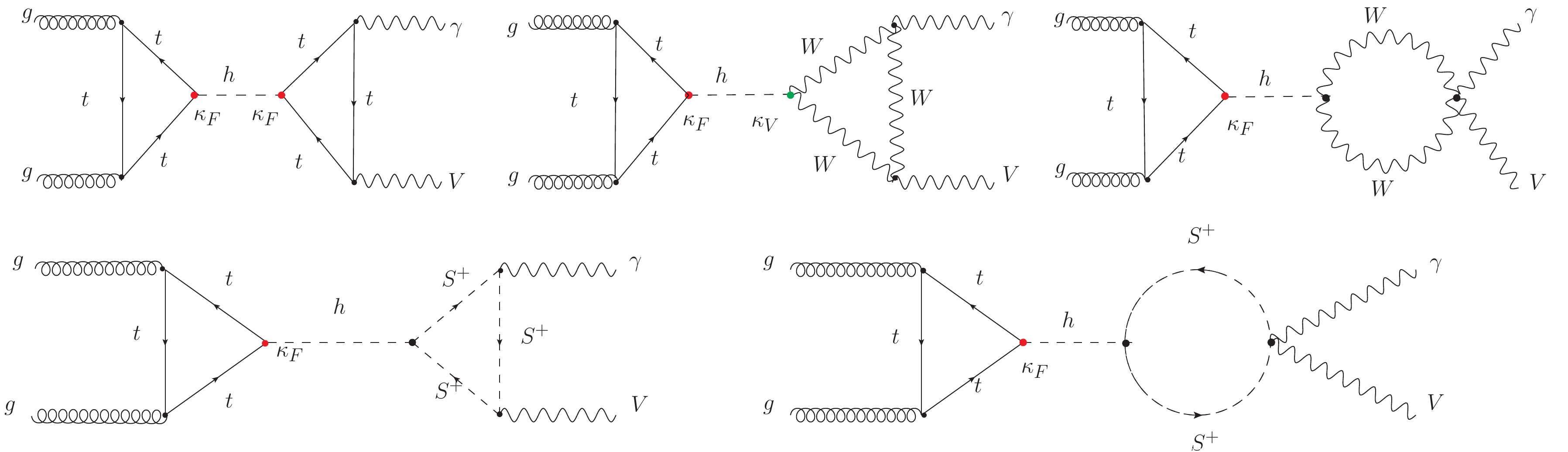
Figure 1: Feynman diagrams relevant to the Higgs decay $h\to\gamma~{}V$ ($V=\gamma,Z$) at the LHC. The red and blue points refer to the vertices that could be modified with respect to the SM by the factors $\kappa_{F}$ and $\kappa_{V}$, respectively.

From the diagrams in Fig. 1, one finds the ratios

$$R_{\gamma\gamma} =\kappa_{F}^{2}\left|\frac{\frac{\upsilon}{2}\sum_{X}\frac{g_{hXX}}{m_{X}^{2}}Q_{X}^{2}A_{0}^{\gamma\gamma}(\tau_{X})+\kappa_{V}A_{1}^{\gamma\gamma}(\tau_{W})+\kappa_{F}\frac{4}{3}A_{1/2}^{\gamma\gamma}(\tau_{t})}{A_{1}^{\gamma\gamma}(\tau_{W})+\frac{4}{3}A_{1/2}^{\gamma\gamma}(\tau_{t})}\right|^{2},$$ (28)

$$R_{\gamma Z} =\kappa_{F}^{2}\left|\frac{\upsilon\sum_{X}\frac{g_{hXX}C_{ZXX}}{m_{X}^{2}}Q_{X}A_{0}^{\gamma Z}(\tau_{X},\lambda_{X})+\kappa_{V}A_{1}^{\gamma Z}(\tau_{W},\lambda_{W})+\kappa_{F}\frac{-6+16s_{\mathrm{w}}^{2}}{3s_{\mathrm{w}}c_{\mathrm{w}}}A_{1/2}^{\gamma Z}(\tau_{t},\lambda_{t})}{A_{1}^{\gamma Z}(\tau_{W},\lambda_{W})+\frac{-6+16s_{\mathrm{w}}^{2}}{3s_{\mathrm{w}}c_{\mathrm{w}}}A_{1/2}^{\gamma Z}(\tau_{t},\lambda_{t})}\right|^{2},$$ (29)

where $X=H_{3}^{+},\,H_{5}^{+},\,H_{5}^{++}$ stands for all charged scalars inside the loop diagrams, $Q_{X}$ is the electric charge of the field $X$ in units of $|e|$, $\tau_{X}=4m_{X}^{2}/m_{h}^{2},~{}\lambda_{X}=4m_{X}^{2}/m_{Z}^{2}$; and the functions $A_{i}^{\gamma\gamma,\gamma Z}$ and coefficients $g_{hXX}$ and $C_{ZXX}$ are given in Appendixes A and B, respectively.

Constraints from the production/decay of the heavy scalar $\eta$

After the discovery of the Higgs boson with $m_{h}=125.25\,\mathrm{GeV}$, efforts have been devoted to search for heavy neutral scalar boson through different channels over a wide mass range. Such results can also be used to impose constraints on models with many neutral scalars such as the GM model.

The two $CP-even$ eigenstates $h$ and $\eta$ are defined through a mixing angle $\alpha$ and $(m_{h}<m_{\eta})$, where the light eigenstate $h$ is identified to be the SM-like Higgs boson with the measured mass $m_{h}=125.25\,\mathrm{GeV}$. Here, the heavy scalar $\eta$ has similar couplings as the SM Higgs boson, but modified with the factors,

$$\zeta_{V}=\frac{g_{\eta VV}^{GM}}{g_{hVV}^{SM}}=s_{\alpha}c_{\beta}+\sqrt{\frac{8}{3}}c_{\alpha}s_{\beta},\,\zeta_{F}=\frac{g_{\eta FF}^{GM}}{g_{hFF}^{SM}}=\frac{s_{\alpha}}{c_{\beta}}.$$ (30)

The partial decay width of the heavy scalar $\eta$ into SM final states can be written as $\Gamma(\eta\to X\overline{X})=\zeta_{X}^{2}\Gamma^{SM}(\eta\to X\overline{X})$, where $\Gamma^{SM}(\eta\to X\overline{X})$ is the Higgs partial decay width estimated at $m_{h}\to m_{\eta}$ Higgs . In addition, there exist other BSM decay channels like $\eta\to hh,H_{3}H_{3},H_{5}H_{5}$ when kinematically allowed. The partial decay width for these channels is given by

$$\Gamma(\eta\to Y\overline{Y})=r_{Y}\frac{\left|g_{\eta Y\overline{Y}}\right|^{2}}{32\pi m_{\eta}}\sqrt{1-4\frac{m_{Y}^{2}}{m_{\eta}^{2}},}$$ (31)

with $Y=h,H_{3}^{0},H_{3}^{\pm},H_{5}^{0},H_{5}^{\pm},H_{5}^{\pm\pm}$, $r_{h,H_{3}^{0},H_{5}^{0}}=1$ and $r_{H_{3}^{\pm},H_{5}^{\pm},H_{5}^{\pm\pm}}=2$. Then, the heavy scalar $\eta$ total decay width can be written as

$$\varGamma_{\eta}^{tot}=\sum_{Y\neq SM}\Gamma(\eta\to Y\overline{Y})+\Gamma_{\eta}^{SM}\sum_{X=SM}\zeta_{Y}^{2}\mathcal{B}^{SM}(\eta\to X\overline{X}),$$ (32)

where $\Gamma_{\eta}^{SM}$ and $\mathcal{B}^{SM}(\eta\to X\overline{X})$ are the Higgs total decay width and branching ratios estimated at $m_{h}\to m_{\eta}$ Higgs . Since the heavy scalar $\eta$ decays into all SM final states, it can be searched at the LHC via the processes: (1) $pp\to\eta\to\mathfrak{\ell\ell,\jmath\jmath,\mathrm{VV}}$ and $pp\to\eta\to hh$. For the first type, we include the recent ATLAS analysis at $13\,\textrm{TeV}$ with $139\,\textrm{fb}^{-1}$ $pp\to\eta\to\tau\tau$ ATLAS:2020zms and $pp\to S\to ZZ$ via the channels $\ell\ell\ell\ell$ and $\ell\ell\nu\nu$ ATLAS:2020tlo . In the other side, when checking the bounds from the decay $pp\to\eta\to WW$, one finds that the recent CMS analyses CMS:2021klu are not convenient to use here, due to the considered large mass range $(m_{\eta}>1\,\textrm{TeV})$ in the analysis. For the second type, we use the recent ATLAS combination ATLAS:2021nps that includes the analyses at $13\,\textrm{TeV}$ with $139\,\textrm{fb}^{-1}$ via the channels $hh\to b\bar{b}\tau\tau$ ATLAS:2021fet , $hh\to b\bar{b}b\bar{b}$ ATLAS:2021ulo and $hh\to b\bar{b}\gamma\gamma$  ATLAS:2021jki .

Here, we can take all the above mentioned analyses to constrain the GM model parameters that are relevant to the heavy scalar $\eta$. We define the cross section of the Heavy scalar $\eta$ in function of the branching ratios and decay width as

$$\sigma(pp\to\eta)\times\mathcal{B}(\eta\to X\overline{X})=\zeta_{F}^{2}\zeta_{X}^{2}\frac{\Gamma_{SM}^{tot}(\eta)}{\Gamma^{tot}(\eta)}\sigma^{SM}(pp\to\eta)\times\mathcal{B}^{SM}(\eta\to X\overline{X}),$$ (33)

where $\mathcal{B}^{SM}(\eta\to X\overline{X})$ are the branching ratios of the heavy scalar $\eta$ decaying into a pair of gauge bosons or fermions via the ggF production mode of $\eta$, $\sigma(pp\to\eta)$ and $\sigma^{SM}(pp\to\eta)$ are the proton-proton collision production cross section.

LHC Constraints on the triplet and fiveplet Scalars

Here, we implement some of the most stringent constraints, especially the vector boson fusion (VBF) production of $H_{5}^{++}$ and the Drell-Yan production of a neutral Higgs boson.

A. VBF $H_{5}^{++}\to W^{+}W^{+}\to$ like sign dileptons

The experimental bound on $s_{H}$ as a function of $m_{5}$ is constrained by a CMS result of $35.9\,\textrm{fb}^{-1}$ of LHC run 2 (13 TeV) data CMS:2017fhs for $m_{5}>200~{}\textrm{GeV}$, we assume that the signal production cross section is proportional to $s_{H}^{2}$ where

$$(s_{H}^{limit})^{2}\times\mathcal{B}(H_{5}^{++}\to W^{+}W^{+})=(s_{H}^{CMS})^{2},$$ (34)

with $(s_{H}^{CMS})^{2}$ is the bound presented at CMS:2017fhs that corresponds to $\mathcal{B}(H_{5}^{++}\to W^{+}W^{+})=1$.

B. Drell-Yan $H_{5}^{0}H_{5}^{\pm}$ with $H_{5}^{0}\to\gamma\gamma$

Concerning the Drell-Yan production of $H_{5}^{0}H_{5}^{\pm}$ with $H_{5}^{0}$, there exist two ATLAS searches for diphoton resonances in the mass range $65<m_{5}<600~{}\textrm{GeV}$ using $20.3\,\textrm{fb}^{-1}$ of LHC run 1 (8 TeV) data ATLAS:2014jdv and of the $36.7\,\textrm{fb}^{-1}$ luminosity of LHC run 2 (13 TeV) data in the mass range $200<m_{5}<2700~{}\textrm{GeV}$ ATLAS:2017ayi . The total cross sections at 8 TeV and 13 TeV for $H_{5}^{0}H_{5}^{+}$ and $H_{5}^{0}H_{5}^{-}$ are shown in Ismail:2020zoz . The fiducial cross section is constrained by the following expression:

$$\sigma_{fiducial}=(\sigma_{H_{5}^{0}H_{5}^{+}}\times\epsilon_{+}+\sigma_{H_{5}^{0}H_{5}^{-}}\times\epsilon_{-})\times\mathcal{B}(H_{5}^{0}\to\gamma\gamma),$$ (35)

where the efficiencies $\epsilon_{\pm}$ for $H_{5}^{0}H_{5}^{\pm}$ respectively, are shown in Ismail:2020zoz . As we will see later, only the 8 TeV constraints are relevant to (35) since the 13 TeV cross section values are 3 orders of magnitude suppressed with respect to the experimental bounds.

The $b\to s$ transition bounds

Since the charged triplet $H_{3}^{\pm}$ is partially coming from the SM doublet as shown in (8), then it couples to the up and down quarks similar to the way the W gauge boson does. These interactions lead to flavor violating processes such as the $b\to s$ transition ones, which depend only on the charged triplet mass $m_{3}$ and the mixing angle $\beta$. The current experimental value of the $b\to s\gamma$ branching ratio, for a photon energy $E_{\gamma}>1.6~{}\textrm{GeV}$ is $\mathcal{B}(\overline{B}\to X_{s}\gamma)_{exp}=(3.55\pm 0.24\pm 0.09)\times 10^{-4}$, while the two SM predictions are $\mathcal{B}(\overline{B}\to X_{s}\gamma)_{SM}=(3.15\pm 0.23)\times 10^{-4}$ Misiak:2006zs and $\mathcal{B}(\overline{B}\to X_{s}\gamma)_{SM}=(2.98\pm 0.26)\times 10^{-4}$ Becher:2006pu . In our numerical scan, we consider the bounds on the $m_{3}$-$\upsilon_{\chi}$ plan shown in Hartling:2014aga .

V Numerical Analysis and Discussion

We perform a numerical scan over the parameter space of the GM model and probe the effect of different theoretical and experimental constraints on the parameter space. We require the light $CP-even$ scalar to be the $125\,\textrm{GeV}$ SM-like Higgs boson and impose the constraints from perturbativity, unitarity, boundness from below, the diphoton Higgs decay, the Higgs total decay width, the Higgs signal strength modifiers, the electroweak precision tests, the constraints from the doubly charged Higgs bosons and Drell-Yan diphoton production, and the indirect constraint from the $b\to s\gamma$ transition processes.

We choose the model free parameters to be $\lambda_{2},\;\lambda_{4},\;m_{\eta},m_{3},\;m_{5},\,s_{\alpha}\;\textrm{and}\;s_{\beta}\equiv\sin\beta=2\sqrt{2}\upsilon_{\xi}/\upsilon$, which lie in the ranges,

$$78~{}\textrm{GeV}<m_{3}<1~{}\textrm{TeV},78~{}\textrm{GeV}<m_{5}<1.8~{}\textrm{TeV},\,m_{h}<m_{\eta}<1~{}\textrm{TeV},\,\left|\lambda_{2,4}\right|\leq 10,\,\left|s_{\beta}\right|\leq 1,$$ (36)

where the triplet and fiveplet charged scalars are subject to a mass lower bound from LEP ALEPH:2013htx . Here, the negative values of $s_{\beta}$ should be considered due to the following reason. In the GM model, we have $V(\Phi,\Delta,\mu_{1,2})=V(\Phi,-\Delta,-\mu_{1,2})$, and therefore all the mass matrix elements are also invariant under this transformation. However, since the scalar eigenstates are mixtures of the components of $\Phi$ and $\Delta$, the physical vertices that involves scalars are not invariant under $(\Phi,\Delta,\mu_{1,2})\to(\Phi,-\Delta,-\mu_{1,2})$. This means that any two BPs with the same input parameters but with opposite signs of $(\pm s_{\beta},\pm\mu_{1,2})$ are physically different. This makes the negative $s_{\beta}$ values in (36) independent parameter space that should not be ignored.

In order to check whether there exist wrong vacua that are deeper than the EW one $(\upsilon_{\phi},\,\sqrt{2}\upsilon_{\xi},\upsilon_{\xi})$, we show in Fig. 2 the scalar mass ranges with (left) and without (right) the condition (15).

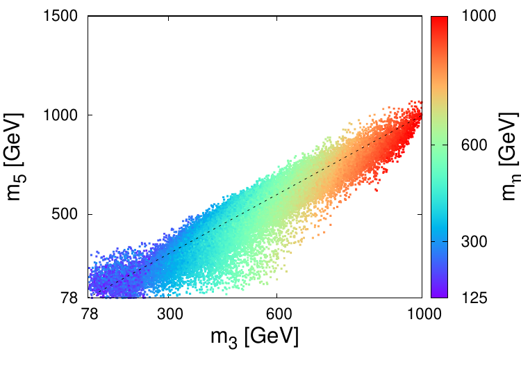
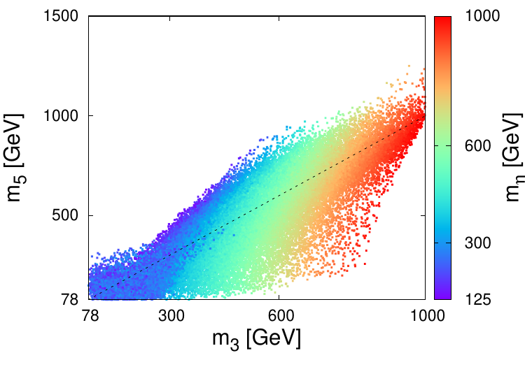
Figure 2: The masses for triplet, fiveplet and singlet $\eta$ estimated in the GM model by considering the basic theoretical and experimental constraints with (left) and without (right) the condition of the EW vacuum to be the deepest (15).

From the 58.5k BPs, 35k BPs fulfill the condition (15). This means that almost 40 % of the parameter space considered in the literature are excluded by the fact that the EW vacuum $(\upsilon_{\phi},\,\sqrt{2}\upsilon_{\xi},\upsilon_{\xi})$ is not the deepest one. Clearly, when considering all the theoretical and experimental constraints except the condition (15), the fiveplet and the singlet $\eta$ masses can reach the values $m_{5}=1.25\,\textrm{TeV}$ and $m_{\eta}=1\,\textrm{TeV}$, respectively for the triplet maximal mass value $m_{3}=1\,\textrm{TeV}$. However, when considering the constraint (15), the fiveplet mass ranges get shrunk as $m_{5}<1.1~{}\textrm{TeV}$. This requires a full reanalysis of different phenomenological aspects of this model. The viable parameter space in Fig. 2-right is a consequence of a combination of the theoretical and experimental constraints mentioned above.

In what follows, we will consider only the 35k viable BPs in our analysis, as shown in Fig. 3

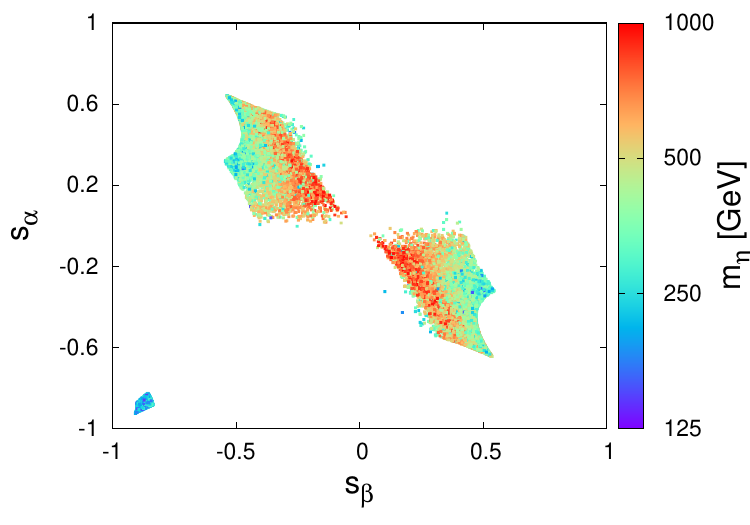
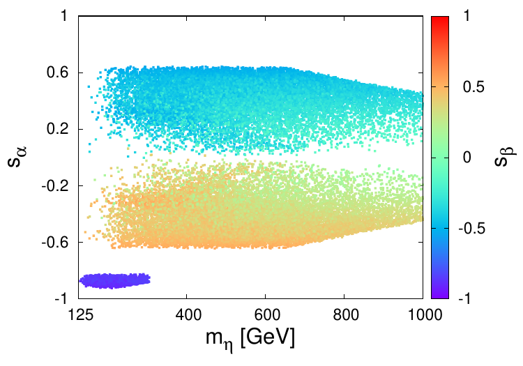
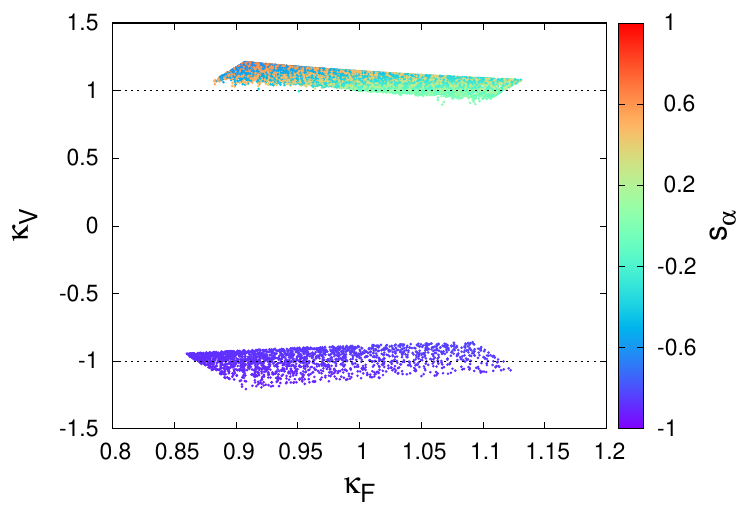
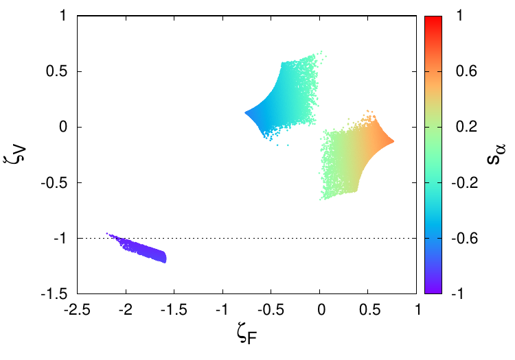
Figure 3: Different physical observables estimated in the GM model by considering the theoretical and experimental constraints, i.e., the BPs used to produce Fig. 2-left.

From Fig. 3, one has to mention that the parameter space is well constrained and split into three isolated islands in the plans of $\{s_{\beta},s_{\alpha}\}$, $\{s_{\alpha},m_{\eta}\}$ and $\{\zeta_{F},\zeta_{V}\}$; and into two islands in the plans of $\{\kappa_{F},\kappa_{V}\}$. For instance, the three islands correspond to the ranges {-0.92$<s_{\beta}<$-0.83, -0.92$<s_{\alpha}<$-0.81}, {-0.54$<s_{\beta}<$-0.05 , 0.01$<s_{\alpha}<$0.64} and {0.04$<s_{\beta}<$0.54, -0.64$<s_{\alpha}<$0.03}, respectively. According to the bottom-right panel in Fig. 3, the $\kappa$’s values for the two islands are {-1.21$<\kappa_{V}<$-0.85, 0.86$<\kappa_{F}<$1.12} and {0.9$<\kappa_{V}<$1.23, 0.88$<\kappa_{F}<$1.13}, respectively. While, the corresponding $\zeta$’s ranges are $\{-1.22<\zeta_{V}<-0.97,~{}-2.15<\zeta_{F}<-1.59\}$, $\{-0.09<\zeta_{V}<0.66,~{}-0.75<\zeta_{F}<-0.02\}$ and $\{-0.65<\zeta_{V}<0.14,~{}0.04<\zeta_{F}<0.75\}$, for the three islands, respectively. Here, the shape of all islands is dictated by the combination of all the above mentioned constraints, however, some of the constraints could have the dominant impact on such a region. For instance, the shape of the isolated islands is mainly dictated by the bounds from $b\to s$.

The Higgs coupling modifier $\kappa_{V}$ is very constrained and could have both signs, while the $\kappa_{F}$ deviation with respect to the SM can reach 13 %. These deviations of $\kappa_{F,V}$ form the SM are possible due to the strength of the bounds from some experimental constraints, such as the diphoton Higgs decay, the bounds on the total Higgs decay width and the Higgs signal strength modifiers. Unlike most of the SM extensions that involve a heavy scalar whose couplings to the fermions and gauge bosons are similar to those of the SM-like Higgs bosons, the scaling factor could have values larger than unity $|\zeta_{F}|>1$. The reason of the significant deviation of the factors $\zeta_{V},\kappa_{V}$ from unity, could be the factor $\sqrt{8/3}$, in addition to the sine and cosine in the denominator in (30) and (22). These values are very similar to the results obtained in Ismail:2020zoz for the region of positive $\kappa_{V}$ due to the stringent constraints from the $b\to s$ transition bounds. However, we got another region with negative $\kappa_{V}$ values that is not mentioned in Ismail:2020zoz , as it is allowed all the constraints considered in our scan of the full free parameters ranges (36).

In the majority of SM scalar extensions where the heavy scalar $\eta$ couplings to the fermions and gauge bosons are much smaller than the SM values ($|\zeta_{F,V}|\ll 1$). This makes these models in agreement with all the negative searches of a heavy resonance. But in the GM model, the situation is different, i.e., $\zeta_{F,V}$ are not suppressed, and these negative searches could play a key role to exclude most of the parameter space as will be seen next.

In Fig. 4, we show the ratios $R_{\gamma\gamma}$ and $R_{\gamma Z}$ for the SM-like Higgs boson (left) and the Higgs total decay width versus its branching ratios (right).

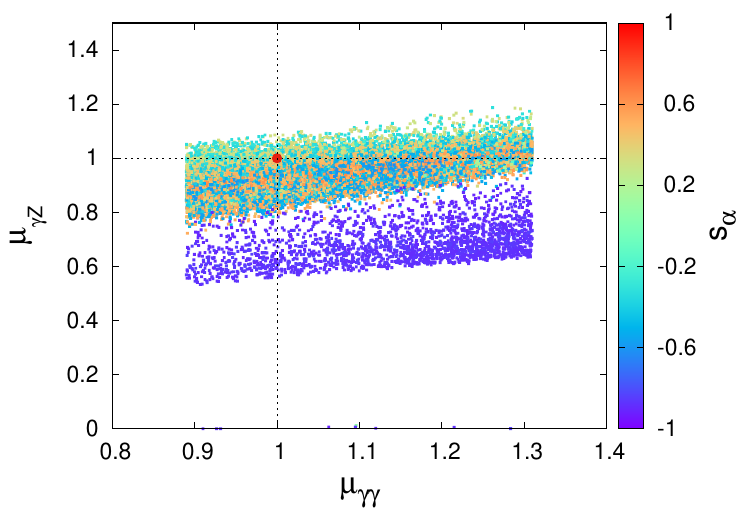
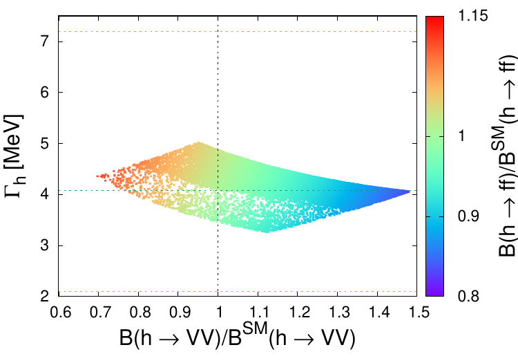
Figure 4: Left: the ratio $R_{\gamma Z}$ in function of $R_{\gamma\gamma}$, where the palette shows the sine of the mixing angle $\alpha$. Right: the SM-like Higgs total decay width versus Higgs branching ratio to gauge bosons scaled by its SM value. The palette shows the Higgs branching ratio to fermions scaled by its SM value; and the dashed line at $\Gamma_{h}=4.08\,\textrm{MeV}$ corresponds to the SM value, while the experimentally allowed values are shown by the dashed lines at $2.1\,\textrm{MeV}$ and $7.2\,\textrm{MeV}$ ATLAS .

From Fig. 4-left, while the values of $R_{\gamma\gamma}$ are constrained by the current LHC data Workman:2022ynf , the ratio $R_{\gamma Z}$ is modified drastically with respect to the SM, it could be reduced by $\sim-45\%$ as it could be $\sim 18\%$ enhanced with respect to the SM. There are few BPs where $R_{\gamma Z}$ is almost null, which correspond to some specific values of $\kappa_{F,V}$, where a possible cancellation could occur between different terms in (29). From the right panel, one learns that the Higgs decays into gauge bosons and fermions can be reduced/enhanced by $-70-150\%$ and $-90-110\%$, respectively. Therefore, more precise Higgs measurements will tighten these ranges and constraint more the parameter space. For the considered parameter space, the oblique parameter given in (27) takes the values $-0.17<\Delta S<0.25$.

In Fig. 5, we present some observables relevant to the heavy scalar $\eta$ versus its mass. In the left panel we show its total decay width and its invisible and undetermined branching fractions in the middle panel, while the SM branching ratios are shown in the right panel.

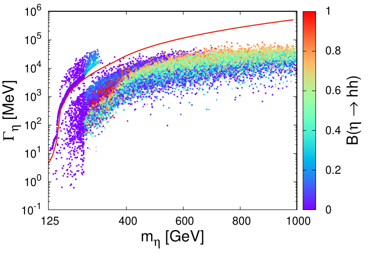
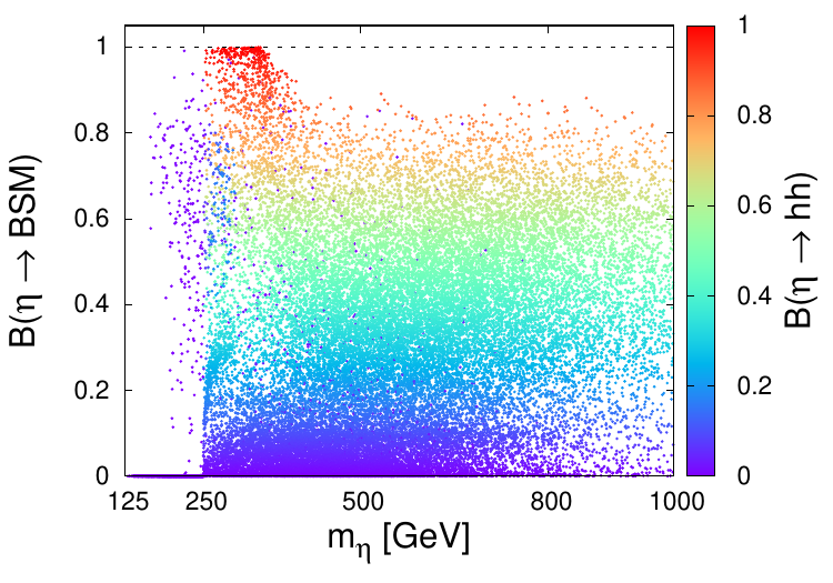
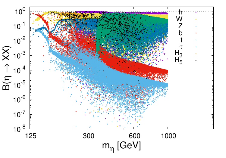
Figure 5: Left: the total decay width of the scalar $\eta$ in function of its mass $m_{\eta}$, where the palette shows its di-Higgs branching ratio. The red curve represents the total decay $\Gamma_{\eta}$ estimated in the SM Higgs , i.e., with $s_{\alpha}=1$ and $B_{BSM}=0$. Middle: the BSM branching ratio $BSM=h,H_{3},H_{5}$ versus $m_{\eta}$, where the palette shows the di-Higgs branching ratio. Right: the branching ratios ${\cal B}(\eta\to XX)$ versus $m_{\eta}$.

One has to mention that the singlet scalar $\eta$ total decay width could be either 2 orders of magnitude smaller or larger than SM estimated value as shown in Fig. 5-left. This can be understood due the possible significant deviation of the factors $\zeta_{F,V}$ from unity, in addition to possible large values for the possible partial decay widths for $\eta\to hh,H_{3}H_{3},H_{5}H_{5}$. According to Fig. 5-middle, one notices that the BSM channels could be dominant for $m_{\eta}>160~{}\textrm{GeV}$. Here, one notes that the BSM branching ratios are dominant by $\eta\to H_{3}H_{3}$ and $\eta\to H_{5}H_{5}$ in the region of mass $145\,\textrm{GeV}<m_{\eta}<250\,\textrm{GeV}$ but when $m_{\eta}>250\,\textrm{GeV}$ the BSM branching ratio is dominant by $\eta\to hh$. Clearly from Fig. 5-right, one remarks that the branching ratios $\mathcal{B}(\eta\to WW,\,ZZ,\,b\overline{b},\,\tau\tau,\,tt)$ are comparable to their SM corresponding values Higgs for a large portion of the BPs.

In Fig. 6, we show the resonant production cross section of the heavy scalar $\eta$ compared to the experimental bounds in the channels $\tau\tau$ (left) and $ZZ$ (right).

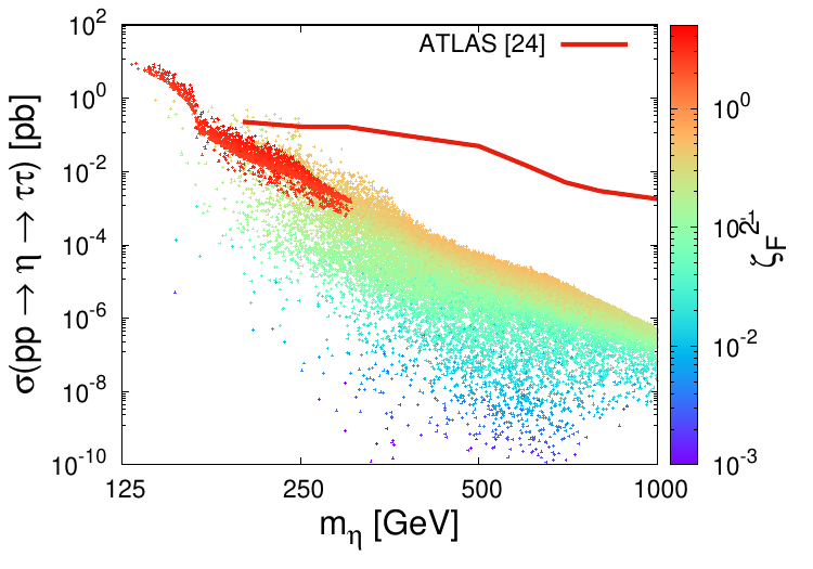
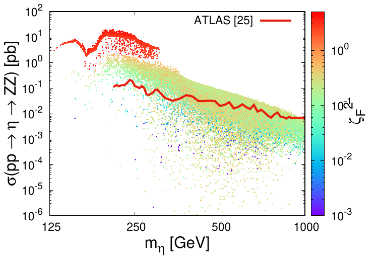
Figure 6: The resonant production cross section $pp\to\eta\to\tau\tau$ (left) and $pp\to\eta\to ZZ$ (right) as a function of the heavy scalar mass $m_{\eta}$, where the palette shows the square of the scaling factor $\zeta_{F}$. The red curves represent the corresponding experimental bounds from ATLAS ATLAS:2020zms ; ATLAS:2020tlo .

From Fig. 6, the experimental bounds from the negative searches for a heavy resonance in the channels $\tau\tau$ and $ZZ$ exclude significant part of the parameter space. However, more regions in the parameter space will be excluded if the future searches for a heavy resonance would consider the mass range $125-200~{}\textrm{GeV}$. For the $\eta\to ZZ$ constraint, if one extrapolates the bound into small $m_{\eta}$ values, one learns that all the BPs with $\zeta_{F}^{2}>0.6$ are excluded.

Concerning the resonant production $\eta\to hh$, the production cross section can not be directly compared to the experimental bounds in the channels $hh\to b\bar{b}\tau\tau$ ATLAS:2021fet , $hh\to b\bar{b}b\bar{b}$ ATLAS:2021ulo and $hh\to b\bar{b}\gamma\gamma$ ATLAS:2021jki , since these analyses have been performed by taking into account the SM Higgs branching ratio. Therefore, the modified cross section

$$\sigma^{mod}(pp\to\eta\to hh)=\sigma^{GM}(pp\to\eta\to hh)\times\frac{\mathcal{B}(h\to X_{1}\bar{X}_{1})\mathcal{B}(h\to X_{2}\bar{X}_{2})}{\mathcal{B}^{SM}(h\to X_{1}\bar{X}_{1})\mathcal{B}^{SM}(h\to X_{2}\bar{X}_{2})},$$ (37)

is the relevant quantity to be compared with the experimental bounds ATLAS:2021fet ; ATLAS:2021ulo ; ATLAS:2021jki in the channel $hh\to X_{1}\bar{X}_{1}X_{2}\bar{X}_{2}$. In Fig. 7, we show the modified cross section (37) as a function of the heavy scalar mass from the combination of $hh\to b\bar{b}\tau\tau$ and $hh\to b\bar{b}\gamma\gamma$ for the BPs with $m_{\eta}>250~{}\textrm{GeV}$, where the palette shows the branching ratio of $\eta\to hh$.

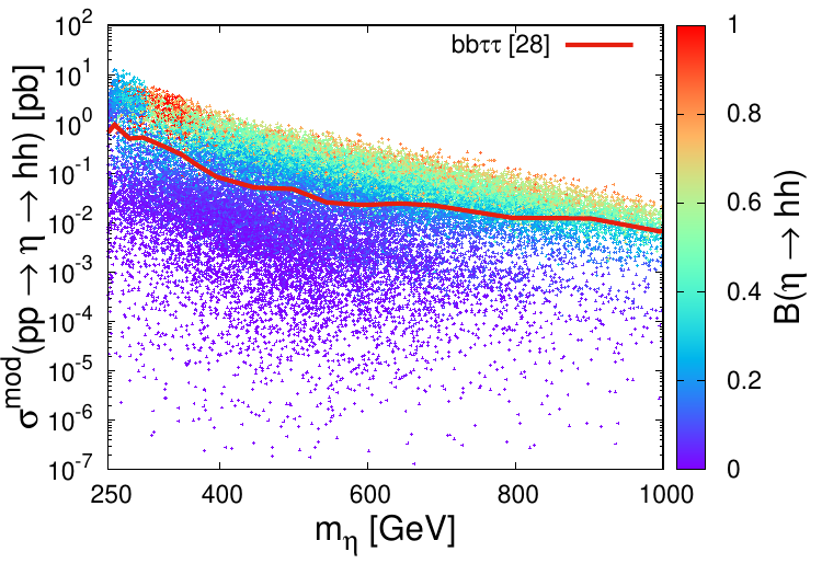
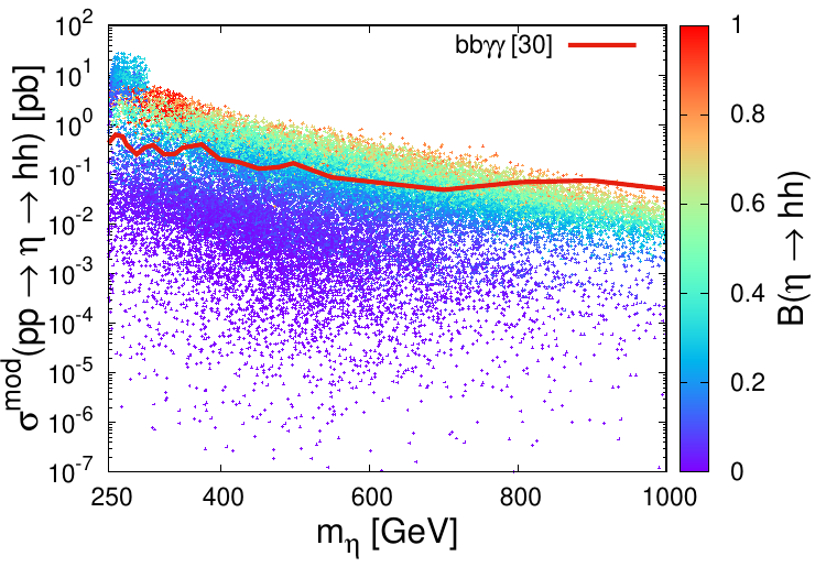
Figure 7: The $hh$ production cross section (37) as a function of $m_{\eta}$ from the combination of $hh\to b\bar{b}\tau\tau$ ATLAS:2021fet , (left) and via $hh\to b\bar{b}\gamma\gamma$ ATLAS:2021jki (right).

From Fig. 7, one learns that the majority of the BPs with $m_{\eta}>250~{}\textrm{GeV}$ are excluded by the experimental bounds ATLAS:2020zms ; ATLAS:2020tlo ; CMS:2021klu ; ATLAS:2021nps ; ATLAS:2021fet ; ATLAS:2021ulo ; ATLAS:2021jki . One has to mention that the di-Higgs negative searches are used to set some limits on the triple Higgs couplings and to constrain the scalar sector in many multiscalar SM extensions, but here in the GM model, the resonant $\eta\to hh$ experimental bounds are very efficient in excluding large part of the parameter space. This point will be investigated in details in a future work next .

Here, in Fig. 8 we show the effect of the constraints from the doubly charged Higgs bosons and Drell-Yan diphoton production on different observables like $s_{\beta}^{2}\times\mathcal{B}(H_{5}^{++}\to W^{+}W^{+})$ and the cross section of the diphoton production at 8 TeV which are plotted in function of $m_{5}$ and the corresponding branching ratio in the palette. One has to mention that it is worthless to show the cross section $pp\to H_{5}^{0}\to\gamma\gamma$ at 13 TeV since the existing experimental bounds are given for the $m_{5}$ range ATLAS:2017ayi , that it is already excluded by previous constraints.

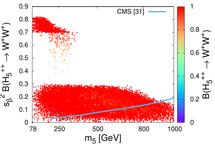
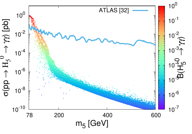
Figure 8: Left: the quantity $s_{\beta}^{2}\times\mathcal{B}(H_{5}^{++}\to W^{+}W^{+})$ in function of $m_{5}$, where the palette shows the branching ratio $\mathcal{B}(H_{5}^{++}\to W^{+}W^{+})$. The blue curve represents the experimental bounds from CMS CMS:2017fhs . Right: the cross section of the diphoton production at 8 TeV, where the palette shows the corresponding branching ratio. The blue curve shows the experimental bound ATLAS:2014jdv . Here, the BPs with $m_{5}>600~{}\textrm{GeV}$ are not considered since by the experimental bound ATLAS:2014jdv were established only for $m_{5}<600~{}\textrm{GeV}$.

One notices from Fig. 8-left that the branching ratio $\mathcal{B}(H_{5}^{++}\to W^{+}W^{+})$ value does not play an important role in excluding the BPs by the experimental bounds CMS:2017fhs ; however, the mixing value $s_{\beta}$ does. From Fig. 8-right, one remarks that most of the diphoton scalar negative searches exclude most of the BPs with $\mathcal{B}(H_{5}^{0}\to\gamma\gamma)>0.09$, which is in good agreement with the experimental bound ATLAS:2014jdv .

In Fig. 9, we reproduce the physical observables shown in Fig. 3 by considering only the BPs that are in agreement with all the above mentioned experimental bounds ATLAS:2020zms ; ATLAS:2020tlo ; CMS:2021klu ; ATLAS:2021nps ; ATLAS:2021fet ; ATLAS:2021ulo ; ATLAS:2021jki fulfill the constraints from doubly charged Higgs boson and Drell-Yan diphoton production, the indirect constraints from the $b\to s$ transition processes and the LHC measurements on the Higgs strengths modifiers.

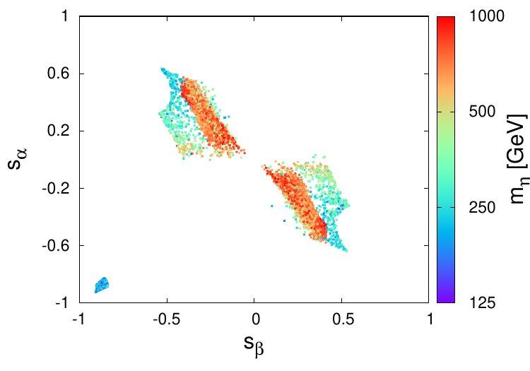
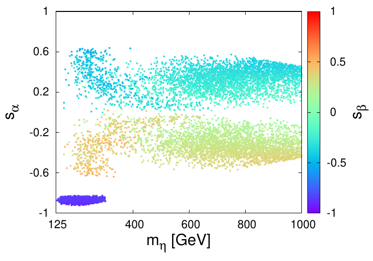
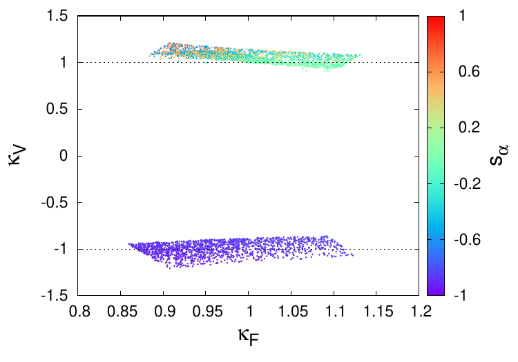
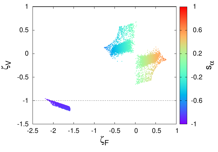
Figure 9: The physical observables that are presented in Fig. 3 reproduced using only BPs that are in agreement with the recent ATLAS and CMS experimental bounds ATLAS:2020zms ; ATLAS:2020tlo ; CMS:2021klu ; ATLAS:2021nps ; ATLAS:2021fet ; ATLAS:2021ulo ; ATLAS:2021jki ; in addition to the constraints from the doubly charged Higgs bosons and Drell-Yan di-photon production CMS:2017fhs ; ATLAS:2014jdv ; ATLAS:2017ayi as well as the indirect constraints from $b\to s\gamma$ and the LHC measurements on the Higgs strengths modifiers.

From the 35k BPs considered in our analysis, 74.5 % are excluded by the above combined constraints, where the majority of BPs correspond to $m_{\eta}<2m_{h}$. However, most of them are not excluded due the absence of the experimental bounds for $m_{5}<200~{}\textrm{GeV}$. By comparing Fig. 9 with Fig. 3, one has to mention that these constraint do not change the shape of the islands described previously.

Before concluding this debate, it is essential to discuss the impact of future measurements at the HL-LHC on this model. The primary objectives of the HL-LHC include enhancing measurements related to the 125 GeV Higgs boson’s couplings, decays, and the search for heavy Higgs particles. Additionally, it offers an important opportunity to test some BSM theories. In a study by Li Li:2018jns , the possibility of observing the type-II seesaw doubly charged scalar was investigated. They obtained a mass upper bound of $655~{}\textrm{GeV}$, which is irrelevant to the doubly charged scalar in the current model. According to the projections for Higgs property measurements TheATLAScollaboration:2014ewu , it is expected that the various Higgs scaling factors and, consequently, the signal strength modifiers in (25) will be measured with significantly improved precision. This will result in narrower experimentally allowed ranges for the scaling factors $\kappa_{F,V}$ as shown in (26), leading to the exclusion of a significant portion of the parameter space.

VI Conclusion

In this work, we have studied the scalar potential of the GM model that preserves custodial SU(2) symmetry. We have considered the theoretical and experimental constraints on the parameter space such as the tree-level unitarity, the potential boundness from below, avoiding possibly deeper wrong minima, the electroweak precision tests, the Higgs total decay width and diphoton decay, and the Higgs strength modifiers, the negative searches on the doubly charged Higgs bosons and the Drell-Yan diphoton production, as well as the indirect constraints from the $b\to s$ transition processes; in addition to the direct searches for additional heavy Higgs resonances.

We performed a numerical scan based on all the above-mentioned theoretical and experimental constraints, and we found that the possible unwanted minima that could be deeper than the EW vacuum excludes about 40 % of the parameter space that fulfills the above mentioned constraints. On top of that, we noticed that the above constraints dictate a clear shape on the model parameter of three separated islands in the plans of $\{s_{\beta},s_{\alpha}\}$, $\{s_{\alpha},m_{\eta}\}$ and $\{\zeta_{F},\zeta_{V}\}$, and two islands in the plans of $\{\kappa_{F},\kappa_{V}\}$. The couplings of the Higgs boson to the gauge bosons and fermions lie in the ranges {-1.21$<\kappa_{V}<$-0.85, 0.86$<\kappa_{F}<$1.12} and {0.9$<\kappa_{V}<$1.23, 0.88$<\kappa_{F}<$1.13}, respectively. However, the scaling factors of the heavy scalar $\eta$ in the GM $\zeta_{F},_{V}$ lie in the ranges {-1.22$<\zeta_{V}<$-0.97, -2.15$<\zeta_{F}<$-1.59}, {-0.09$<\zeta_{V}<$0.66, -0.75$<\zeta_{F}<$-0.02} and {-0.65$<\zeta_{V}<$0.14, 0.04$<\zeta_{F}<$0.75}, respectively. Here, an isolated islands in the plans of that was supposed to exist was excluded by the $b\to s$ bound. The shape of the isolated islands as shown in the plans of $\{s_{\beta},s_{\alpha}\}$, $\{s_{\alpha},m_{\eta}\}$, $\{\zeta_{F},\zeta_{V}\}$ and $\{\kappa_{F},\kappa_{V}\}$ is dictated by the combination of the bounds of the Higgs signal strength modifiers and the Higgs total decay width; in addition to the Higgs diphoton decay.

We have also imposed the constraints from the negative searches of both doubly charged Higgs bosons in the VBF channel and Drell-Yan diphoton production, where we found that a significant part of the parameter space is excluded by the CMS bound on $s_{\beta}^{2}\times\mathcal{B}(H_{5}^{++}\to W^{+}W^{+})$ CMS:2017fhs . Here, it has been found that the branching ratio of $H_{5}^{++}\to W^{+}W^{+}$ does not play an important role in allowing/excluding any BP, but the mixing $s_{\beta}$ does. Unfortunately, the recent bounds from CMS CMS:2017fhs and ATLAS ATLAS:2017ayi do not cover the mass range $m_{5}<200~{}\textrm{GeV}$, which makes a large part of the parameter space unconstrained by this severe bound. It will be interesting if future analyses would consider this mass range.

The indirect constraints from the $b\to s$ transition processes are also applied and put constraints on the two parameters $m_{3}$ and $\upsilon_{\xi}$ only. We found also that the recent LHC measurements on the Higgs strengths modifiers impose strong constraints on the parameter space, especially the Higgs coupling modifiers $\kappa_{F,V}$. In fact, the direct searches generally provide more strict constraints on the GM model parameter space and open the possibility of a discovery as these searches would be improved within the current/future LHC data. We have imposed also the recent ATLAS and CMS negative searches for the heavy scalar $\eta$ in different channels. We found that the channel $\eta\to hh$ is very useful to exclude most of the parameter space, while, other channels are less efficient since the mass range $125~{}\textrm{GeV}<m_{\eta}<200~{}\textrm{GeV}$ is not covered by most of the searches. Clearly, future searches and more precise measurements will tighten the parameter space of the GM model.

Appendix A FUNCTIONS

The loop functions used in (27) are given by

$$f_{1}(x,\,y) =\frac{5(y^{6}-x^{6})+27(x^{4}y^{2}-x^{2}y^{4})+12(x^{6}-3x^{4}y^{2})\log x+12(3x^{2}y^{4}-y^{6})\log y}{36(y^{2}-x^{2})^{3}},$$

$$f_{3}(x,\,y) =\frac{x^{4}-y^{4}+2x^{2}y^{2}(\log y^{2}-\log x^{2})}{2(x^{2}-y^{2})^{3}},$$ (38)

while those used in (28) and (29) are given by Djouadi:2005gj

$$A_{1}^{\gamma\gamma}(\tau) =2+3\tau+3\tau(2-\tau)f(\tau),~{}A_{1/2}^{\gamma\gamma}(\tau)=-2\tau[1+(1-\tau)f(\tau)],~{}A_{0}^{\gamma\gamma}(\tau)=\tau[1-\tau f(\tau)],$$

$$A_{1}^{\gamma Z}(\tau,\lambda) =-\cot\theta_{W}\big{(}4(3-\tan^{2}\theta_{W})I_{2}(\tau,\lambda)+[(1+\frac{2}{\tau})\tan^{2}\theta_{W}-(5+\frac{2}{\tau})]I_{1}(\tau,\lambda))\big{)},$$

$$A_{1/2}^{\gamma Z}(\tau,\lambda) =I_{1}(\tau,\lambda)-I_{2}(\tau,\lambda),~{}A_{0}^{\gamma Z}(\tau,\lambda)=I_{1}(\tau,\lambda)$$

$$I_{1}(a,\,b) =\frac{ab}{2(a-b)}+\frac{a^{2}b^{2}}{2(a-b)^{2}}[f(a)-f(b)]+\frac{a^{2}b}{(a-b)^{2}}[g(a)-g(b)],$$

$$I_{2}(a,\,b) =-\frac{ab}{2(a-b)}[f(a)-f(b)],$$ (39)

with

$$f(\tau)=\begin{cases}[\arcsin\big{(}\sqrt{\frac{1}{\tau}}\big{)}]^{2}&if\;\tau\geq 1,\\ -\frac{1}{4}\Big{[}\log\big{(}\frac{1+\sqrt{1-\tau}}{1-\sqrt{1-\tau}}\big{)}-i\pi\Big{]}^{2}&\,\,\,\,if\;\tau<1\end{cases},\,\,\,\,\,\,\,\,\,\,\,g(\tau)=\begin{cases}\sqrt{\tau-1}[\sin^{-1}(\sqrt{\frac{1}{\tau}})]&if\;\tau\geq 1,\\ \frac{1}{2}\sqrt{\tau-1}[\log(\frac{\eta_{+}}{\eta_{-}})-i\pi]&if\;\tau<1.\end{cases}$$ (40)

Appendix B COUPLINGS

Here, we give the couplings used in different observables definitions. The couplings that are used in (27) are

$$g_{ZhH_{3}^{0}} =-i\sqrt{\frac{2}{3}}\frac{e}{s_{W}c_{W}}(s_{\alpha}c_{\beta}+\sqrt{\frac{3}{8}}c_{\alpha}s_{\beta}),\,g_{Z\eta H_{3}^{0}}=\mathfrak{i}\sqrt{\frac{2}{3}}\frac{e}{s_{W}c_{W}}(c_{\alpha}c_{\beta}-\sqrt{\frac{3}{8}}s_{\alpha}s_{\beta}),\,g_{ZH_{5}^{0}H_{3}^{0}}=-\mathfrak{i}\sqrt{\frac{1}{3}}\frac{e}{s_{W}c_{W}}c_{\beta},$$

$$g_{ZZ\eta} =\frac{e^{2}}{2s_{W}^{2}c_{W}^{2}}(s_{\alpha}c_{\beta}+\sqrt{\frac{8}{3}}c_{\alpha}s_{\beta}),\,g_{ZZh}=\frac{e^{2}}{2s_{W}^{2}c_{W}^{2}}(c_{\alpha}c_{\beta}-\sqrt{\frac{8}{3}}s_{\alpha}s_{\beta}),\,g_{ZH_{5}^{+}H_{3}^{-}}=\frac{e}{2s_{W}c_{W}}c_{\beta},$$

$$g_{ZZH_{5}^{0}} =-\frac{1}{\sqrt{3}}\frac{e^{2}}{s_{W}^{2}c_{W}^{2}}s_{\beta}\upsilon,\,g_{ZW^{+}H_{5}^{-}}=-\frac{e^{2}}{2s_{W}^{2}c_{W}}s_{\beta}\upsilon,\,g_{ZZh}^{SM}=\frac{e^{2}}{2s_{W}^{2}c_{W}^{2}}\upsilon.$$ (41)

Here, $g_{ZZh}^{SM}$ is the SM coupling. The couplings $g_{hXX,\eta XX}$ used in (28), (29) and (31) are

$$g_{hH_{5}^{++}H_{5}^{--}} =g_{hH_{5}^{+}H_{5}^{-}}=-8\sqrt{3}(\lambda_{3}+\lambda_{4})\upsilon_{\xi}s_{\alpha}+(4\lambda_{2}+\lambda_{5})\upsilon_{\phi}c_{\alpha}-2\sqrt{3}\mu_{2}s_{\alpha},$$

$$g_{hH_{3}^{+}H_{3}^{-}} =-\frac{8}{\sqrt{3}}\Big{(}\frac{\sqrt{2}}{4}\lambda_{5}s_{\beta}c_{\beta}\upsilon_{\phi}+((\lambda_{3}+3\lambda_{4})\upsilon_{\xi}-\frac{3\mu_{2}}{4})c_{\beta}^{2}+\frac{3}{2}(\lambda_{2}+\frac{\lambda_{5}}{6})\upsilon_{\xi}+\frac{\mu_{1}}{24})s_{\beta}^{2}\Big{)}s_{\alpha}$$

$$+2\sqrt{2}c_{\alpha}c_{\beta}s_{\beta}(\lambda_{5}\upsilon_{\xi}+\frac{\mu_{1}}{2})+4c_{\alpha}\Big{(}((\lambda_{2}-\frac{\lambda_{5}}{4})c_{\beta}^{2}+2\lambda_{1}s_{\beta}^{2})\upsilon_{\phi}\Big{)},$$

$$g_{\eta hh} =-2\sqrt{3}c_{\alpha}\Big{(}((\lambda_{5}-2\lambda_{2})\upsilon_{\xi}+\frac{\mu_{1}}{4})c_{\alpha}^{2}-4s_{\alpha}^{2}((\lambda_{3}+3\lambda_{4}+\frac{\lambda_{5}}{2}-\lambda_{2})\upsilon_{\xi}+\frac{\mu_{1}}{8}-\frac{\mu_{2}}{2})\Big{)}$$

$$+4s_{\beta}\Big{(}(\lambda_{5}+6\lambda_{1}-2\lambda_{2})c_{\alpha}^{2}-\frac{s_{\alpha}^{2}}{2}(\lambda_{5}-2\lambda_{2})\Big{)}\upsilon_{\phi},$$

$$g_{\eta H_{5}^{++}H_{5}^{--}} =g_{\eta H_{5}^{+}H_{5}^{-}}=g_{\eta H_{5}^{0}H_{5}^{0}}=8\sqrt{3}(\lambda_{3}+\lambda_{4})\upsilon_{\xi}s_{\alpha}+(4\lambda_{2}+\lambda_{5})\upsilon_{\phi}c_{\alpha}+2\sqrt{3}\mu_{2}s_{\alpha},$$

$$g_{\eta H_{3}^{+}H_{3}^{-}} =g_{\eta H_{3}^{0}H_{3}^{0}}=\frac{8}{\sqrt{3}}\Big{(}\frac{\sqrt{2}}{4}\lambda_{5}c_{\beta}s_{\beta}\upsilon_{\phi}+((\lambda_{3}+3\lambda_{4})\upsilon_{\xi}-\frac{3\mu_{2}}{4})c_{\beta}^{2}+\frac{3}{2}((\lambda_{2}+\frac{\lambda_{5}}{6})\upsilon_{\xi}+\frac{\mu_{1}}{24})s_{\beta}^{2}\Big{)}c_{\alpha}$$

$$+2\sqrt{2}s_{\alpha}c_{\beta}s_{\beta}(\lambda_{5}\upsilon_{\xi}+\frac{\mu_{1}}{2})+4s_{\alpha}\Big{(}(\lambda_{2}-\frac{\lambda_{5}}{4})c_{\beta}^{2}+2\lambda_{1}s^{2})\upsilon_{\phi}\Big{)},$$ (42)

The coefficients $C_{ZXX}$ used in (29) are given by

$$C_{ZH_{5}^{++}H_{5}^{--}} =\frac{1-2s_{W}^{2}}{s_{W}c_{W}},~{}C_{ZH_{3}^{+}H_{3}^{-}}=C_{ZH_{5}^{+}H_{5}^{-}}=\frac{1-2s_{W}^{2}}{2s_{W}c_{W}}.$$ (43)

Appendix C WRONG MINIMA

The GM scalar potential may have other minima than the EW one. It is possible to get analytic formula for some these wrong minima, like the ones below, but others require numerical efforts. The following minima are possible only if the quantities inside the square-root are positive.

In the $CP-even$ subspace: we have eight possible minima that corresponds to $V_{i}^{0+}$,

$$\begin{array}[]{cc}\{h_{\phi},\,h_{\chi},\,h_{\xi}\}&=\Big{(}\pm\frac{\sqrt{-\lambda_{1}m_{1}^{2}}}{2\lambda_{1}},0,0\Big{)},\,\Big{(}0,\pm\frac{\sqrt{-2m_{2}^{2}(2\lambda_{4}+\lambda_{3})}}{2(2\lambda_{4}+\lambda_{3})},0\Big{)},\\ &\Big{(}0,0,\pm\frac{\sqrt{-m_{2}^{2}(\lambda_{4}+\lambda_{3})}}{2(\lambda_{4}+\lambda_{3})}\Big{)},\ \Big{(}0,\frac{1}{\lambda_{3}}\sqrt{\frac{-m_{2}^{2}\lambda_{3}^{2}-9\mu_{2}^{2}\lambda_{3}-9\mu_{2}^{2}\lambda_{4}}{2\lambda_{3}+4\lambda_{4}}},-\frac{3\mu_{2}}{2\lambda_{3}}\Big{)},\\ &\Big{(}0,\,\pm\frac{\sqrt{3\mu_{2}\sqrt{-4m_{2}^{2}\lambda_{3}-12m_{2}^{2}\lambda_{4}+9\mu_{2}^{2}}-2m_{2}^{2}\lambda_{3}-6m_{2}^{2}\lambda_{4}+9\mu_{2}^{2}}}{2\lambda_{3}+6\lambda_{4}},\,\frac{3\mu_{2}+\sqrt{-4m_{2}^{2}\lambda_{3}-12m_{2}^{2}\lambda_{4}+9\mu_{2}^{2}}}{4\lambda_{3}+12\lambda_{4}}\Big{)},\\ &\Big{(}0,\,\pm\frac{\sqrt{-3\mu_{2}\sqrt{-4m_{2}^{2}\lambda_{3}-12m_{2}^{2}\lambda_{4}+9\mu_{2}^{2}}-2m_{2}^{2}\lambda_{3}-6m_{2}^{2}\lambda_{4}+9\mu_{2}^{2}}}{2\lambda_{3}+6\lambda_{4}},\,\frac{3\mu_{2}+\sqrt{-4m_{2}^{2}\lambda_{3}-12m_{2}^{2}\lambda_{4}+9\mu_{2}^{2}}}{4\lambda_{3}+12\lambda_{4}}\Big{)},\\ &\Big{(}0,\,\pm\frac{\sqrt{3\mu_{2}\sqrt{-4m_{2}^{2}\lambda_{3}-12m_{2}^{2}\lambda_{4}+9\mu_{2}^{2}}-2m_{2}^{2}\lambda_{3}-6m_{2}^{2}\lambda_{4}+9\mu_{2}^{2}}}{2\lambda_{3}+6\lambda_{4}},\,-\frac{-3\mu_{2}+\sqrt{-4m_{2}^{2}\lambda_{3}-12m_{2}^{2}\lambda_{4}+9\mu_{2}^{2}}}{4\lambda_{3}+12\lambda_{4}}\Big{)},\\ &\Big{(}0,\,\pm\frac{\sqrt{-3\mu_{2}\sqrt{-4m_{2}^{2}\lambda_{3}-12m_{2}^{2}\lambda_{4}+9\mu_{2}^{2}}-2m_{2}^{2}\lambda_{3}-6m_{2}^{2}\lambda_{4}+9\mu_{2}^{2}}}{2\lambda_{3}+6\lambda_{4}},\,-\frac{-3\mu_{2}+\sqrt{-4m_{2}^{2}\lambda_{3}-12m_{2}^{2}\lambda_{4}+9\mu_{2}^{2}}}{4\lambda_{3}+12\lambda_{4}}\Big{)}.\end{array}$$ (44)

In the $CP-odd$ subspace: we got three possible minima that corresponds to $V_{i}^{0-}$,

$$\{a_{\phi},\,a_{\chi}\} =\Big{(}\pm\frac{\sqrt{-\lambda_{1}m_{1}^{2}}}{2\lambda_{1}},0\Big{)},~{}\Big{(}0,\pm\frac{\sqrt{-2m_{2}^{2}(2\lambda_{4}+\lambda_{3})}}{2(2\lambda_{4}+\lambda_{3})}\Big{)},$$

$$\Big{(}\sqrt{\frac{-8m_{1}^{2}\lambda_{3}-16m_{1}^{2}\lambda_{4}+8m_{2}^{2}\lambda_{2}-2m_{2}^{2}\lambda_{5}}{32\lambda_{1}\lambda_{3}+64\lambda_{1}\lambda_{4}-16\lambda_{2}^{2}+8\lambda_{2}\lambda_{5}-\lambda_{5}^{2}}},\,\sqrt{\frac{8m_{1}^{2}\lambda_{2}-2m_{1}^{2}\lambda_{5}-16m_{2}^{2}\lambda_{1}}{32\lambda_{1}\lambda_{3}+64\lambda_{1}\lambda_{4}-16\lambda_{2}^{2}+8\lambda_{2}\lambda_{5}-\lambda_{5}^{2}}}\Big{)}.$$ (45)

In the singly charged subspace: in this direction, we parametrized the charged fields as $X^{\pm}=|X|e^{\pm i\varrho}$, and then we found that the minima that correspond to $V_{i}^{\pm}$ do not depend on the phases, i.e.,

$$\begin{array}[]{cc}\{|\phi^{\pm}|,\,|\chi^{\pm}|,\,|\xi^{\pm}|\}&=\Big{(}\pm\frac{\sqrt{-2\lambda_{1}m_{1}^{2}}}{4\lambda_{1}},0,0\Big{)},\,\Big{(}0,\pm\frac{\sqrt{-2m_{2}^{2}(\lambda_{4}+\lambda_{3})}}{4(\lambda_{4}+\lambda_{3})},0\Big{)},\,\Big{(}0,0,\pm\frac{\sqrt{-2m_{2}^{2}(\lambda_{4}+\lambda_{3})}}{4(\lambda_{4}+\lambda_{3})}\Big{)},\\ &\left(\sqrt{\frac{\lambda_{2}m_{1}^{2}-2\lambda_{1}m_{2}^{2}}{16\lambda_{1}\lambda_{3}+16\lambda_{1}\lambda_{4}-4\lambda_{2}^{2}}},\sqrt{\frac{-2\lambda_{3}m_{1}^{2}-2\lambda_{4}m_{1}^{2}+\lambda_{2}m_{2}^{2}}{16\lambda_{1}\lambda_{3}+16\lambda_{1}\lambda_{4}-4\lambda_{2}^{2}}},0\right),\left(\sqrt{\frac{-m_{2}^{2}}{16\lambda_{4}+8\lambda_{3}}},0,\sqrt{\frac{-m_{2}^{2}}{16\lambda_{4}+8\lambda_{3}}}\right),\\ &\left(0,\sqrt{\frac{-2\lambda_{3}m_{1}^{2}-2\lambda_{4}m_{1}^{2}+\lambda_{2}m_{2}^{2}}{16\lambda_{1}\lambda_{3}+16\lambda_{1}\lambda_{4}-4\lambda_{2}^{2}}},\sqrt{\frac{\lambda_{2}m_{1}^{2}-2\lambda_{1}m_{2}^{2}}{16\lambda_{1}\lambda_{3}+16\lambda_{1}\lambda_{4}-4\lambda_{2}^{2}}}\right).\end{array}$$ (46)

In the doubly charged subspace: in the doubly charged directions we have only one possible minimum, which is given by

$$|\chi^{\pm\pm}|=\frac{\sqrt{-m_{2}^{2}(2\lambda_{4}+\lambda_{3})}}{2(2\lambda_{4}+\lambda_{3})}.$$ (47)

Acknowledgements: We would like to thank Abdesslam Arhrib for his valuable comments. The work of A.A. is funded by the University of Sharjah under the Research Projects No. 21021430107 “Hunting for New Physics at Colliders” and No. 23021430135 “Terascale Physics: Colliders vs Cosmology”.

References

• (1) G. Aad et al. (ATLAS Collaboration), Phys. Lett. B 716, 1 (2012);
S. Chatrchyan et al. (CMS Collaboration), Phys. Lett. B 716 30 (2012).
• (2) G. Bertone, D. Hooper, and J. Silk, Phys. Rep. 405, 279 (2005).
• (3) Y. Fukuda et al. (Super-Kamiokande Collaboration), Phys. Rev. Lett. 81, 1562 (1998).
• (4) H. Georgi and M. Machacek, Nucl. Phys. B262, 463 (1985).
• (5) R. L. Workman et al. (Particle Data Group), Prog. Theor. Exp. Phys. 2022, 083C01 (2022).
• (6) A. Ahriche, Phys. Rev. D 107, 015006 (2023).
• (7) C. W. Chiang, A. L. Kuo, and K. Yagyu, J. High Energy Phys. 10 (2013) 072.
• (8) M. S. Chanowitz and M. Golden, Phys. Lett. 165B, 105 (1985); J. F. Gunion, R. Vega, and J. Wudka, H. E. Haber and H. E. Logan, Phys. Rev. D 62, 015011 (2000); M. Aoki and S. Kanemura, Phys. Rev. D 77, 095009 (2008); 89, 059902(E) (2014); S. Godfrey and K. Moats, Phys. Rev. D 81, 075026 (2010); I. Low and J. Lykken, J. High Energy Phys. 10, (2010) 053; H. E. Logan and M. A. Roy, Rev. D 82, 115011 (2010); S. Chang, C. A. Newby, N. Raj, and C. Wanotayaroj, Phys. Rev. D 86, 095015 (2012); S. Kanemura, M. Kikuchi, and K. Yagyu, Phys. Rev. D 88, 015020 (2013); C. Englert, E. Re, and M. Spannowsky, Rev. D 87, 095014 (2013); R. Killick, K. Kumar, and H. E. Logan, Phys. Rev. D 88, 033015 (2013); C. Englert, E. Re, and M. Spannowsky, 035024 (2013); C. W. Chiang, arXiv:1504.06424; C. Degrande, K. Hartling, and H. E. Logan, Phys. Rev. D 96, 075013 (2017); 98, 019901(E) (2018); N. Ghosh, S. Ghosh, and I. Saha, Phys. Rev. D 101, 015029 (2020); D. Das and I. Saha, Phys. Rev. D 98 095010 (2018); A. Ismail, B. Keeshan, H. E. Logan, and Y. Wu, Phys. Rev. D 103, 095010 (2021); A. Ismail, H. E. Logan, and Y. Wu, arXiv:2003.02272; C. Wang, J. Q. Tao, M. A. Shahzad, G. M. Chen, and S. Gascon-Shotkin, arXiv:2204.09198; A. Ismail, B. Keeshan, H. E. Logan, and Y. Wu, Phys. Rev. D 103, 095010; A. Adhikary, N. Chakrabarty, I. Chakraborty, and J. Lahiri, Eur. Phys. J. C 816, 554 (2021).
• (9) K. Hartling, K. Kumar, and H. E. Logan,Phys. Rev. D 90, 015007 (2014).
• (10) S. L. Chen, A. Dutta Banik, and Z. K. Liu, Nucl. Phys. B966, 115394 (2021).
• (11) T. Pilkington, arXiv:1711.04378.
• (12) C. W. Chiang and T. Yamada, Phys. Lett. B 735, 295 (2014); R. Zhou, W. Cheng, X. Deng, L. Bian, and Y. Wu, J. High Energy Phys. 01 (2019) 216; T. K. Chen, C. W. Chiang, C. T. Huang, and B. Q. Lu, arXiv:2205.02064.
• (13) A. Ismail, H. E. Logan, and Y. Wu, arXiv:2003.02272.
• (14) K. Hartling, K. Kumar, and H. E. Logan, Phys. Rev. D 91, 015113 (2015).
• (15) C. W. Chiang, G. Cottin, and O. Eberhardt, Phys. Rev. D 99, 015001 (2019).
• (16) G. Moultaka and M. C. Peyranre, Phys. Rev. D 103, 115006 (2021).
• (17) J. Baron et al. (ACME Collaboration), Science 343, 269 (2014).
• (18) D. Azevedo, P. Ferreira, H. E. Logan, and R. Santos, J. High Energy Phys 03 (2021) 221.
• (19) A. Arhrib, R. Benbrik, M. Chabab, G. Moultaka, M. C. Peyranere, L. Rahili and J. Ramadan, Phys. Rev. D 84, 095005 (2011).
• (20) Evidence of off-shell Higgs boson production and constraints on the total width of the Higgs boson in the $ZZ\to 4\ell$ and $ZZ\to 2\ell 2\nu$ decay channels with the ATLAS detector, Report No. ATLAS-CONF-2022-068.
• (21) G. Abbiendi et al. (ALEPH, DELPHI, L3, OPAL and LEP Collaborations), Eur. Phys. J. C 73, 2463 (2013).
• (22) M. Baak et al. (Gfitter Group), Eur. Phys. J. C 74, 3046 (2014).
• (23) https://twiki.cern.ch/twiki/bin/view/LHCPhysics/LHCHWG.
• (24) G. Aad et al. (ATLAS Collaboration), Phys Rev. Lett. 125, 051801 (2020).
• (25) G. Aad et al. (ATLAS Collaboration), Eur. Phys. J. C 81, 332 (2021).
• (26) A. Tumasyan et al. (CMS Collaboration), Phys. Rev. D 105, 032008 (2022).
• (27) (ATLAS Collaboration), Summary of non-resonant and resonant Higgs boson pair searches from the ATLAS experiment, Report No. ATL-PHYS-PUB-2021-031.
• (28) ATLAS Collaboration, Search for resonant and non-resonant Higgs boson pair production in the $b\bar{b}\tau^{+}\tau^{-}$ decay channel using 13 TeV $pp$ collision data from the ATLAS detector, Report No. ATLAS-CONF-2021-030.
• (29) ATLAS Collaboration, Search for resonant pair production of Higgs bosons in the $b\bar{b}b\bar{b}$ final state using $pp$ collisions at $\sqrt{s}$ = 13 TeV with the ATLAS detector, Report No. ATLAS-CONF-2021-035.
• (30) ATLAS Collaboration, Search for Higgs boson pair production in the two bottom quarks plus two photons final state in $pp$ collisions at $\sqrt{s}=13$ TeV with the ATLAS detector, Report No. ATLAS-CONF-2021-016.
• (31) A. M. Sirunyan et al. (CMS Collaboration), Phys. Rev. Lett. 120, 081801 (2018).
• (32) G. Aad et al. (ATLAS Collaboration), Phys. Rev. Lett. 113, 171801 (2014).
• (33) M. Aaboud et al. (ATLAS Collaboration), Phys. Lett. B 775, 105 (2017).
• (34) M. Misiak, H. M. Asatrian, K. Bieri, M. Czakon, A. Czarnecki, T. Ewerth, A. Ferroglia, P. Gambino, M. Gorbahn, C. Greub, et al., Phys. Rev. Lett. 98, 022002 (2007).
• (35) T. Becher and M. Neubert, Phys. Rev. Lett. 98, 022003 (2007).
• (36) A. Ahriche, The Di-Higgs Production at the LHC in the Georgi-Machacek Model, (to be published).
• (37) A. Djouadi, Phys. Rept. 459, 1 (2008).
• (38) T. Li, J. High Energy Phys. 09 (2018), 079.
• (39) Projections for measurements of Higgs boson signal strengths and coupling parameters with the ATLAS detector at a HL-LHC, Report No. ATL-PHYS-PUB-2014-016.