Joint Sequential Detection and Isolation
for Dependent Data Streams

Abstract

The problem of joint sequential detection and isolation is considered in the context of multiple, not necessarily independent, data streams. A multiple testing framework is proposed, where each hypothesis corresponds to a different subset of data streams, the sample size is a stopping time of the observations, and the probabilities of four kinds of error are controlled below distinct, user-specified levels. Two of these errors reflect the detection component of the formulation, whereas the other two the isolation component. The optimal expected sample size is characterized to a first-order asymptotic approximation as the error probabilities go to 0. Different asymptotic regimes, expressing different prioritizations of the detection and isolation tasks, are considered. A novel, versatile family of testing procedures is proposed, in which two distinct, in general, statistics are computed for each hypothesis, one addressing the detection task and the other the isolation task. Tests in this family, of various computational complexities, are shown to be asymptotically optimal under different setups. The general theory is applied to the detection and isolation of anomalous, not necessarily independent, data streams, as well as to the detection and isolation of an unknown dependence structure.

and

1 Introduction

The field of sequential analysis deals with statistical procedures whose sample size is not fixed in advance, but it is a function of the collected observations. For recent textbooks regarding developments on this area since the groundbreaking work of Abraham Wald [45, 46], we refer to [37, 6]. While earlier works, like Wald’s, were motivated by problems in inspection sampling and quality control, in modern industrial and engineering setups it is quite common that there are multiple data streams that are generated by a multitude of data sources (e.g., sensors, channels, etc.), are monitored sequentially, and need to be utilized for real-time decisions. This is the case, for example, in multiple access wireless network [31], multisensor surveillance systems [18], multichannel signal detection [41], environmental monitoring [32], blind source separation [26], biometric authentication [3], sensor networks [1], power systems [8], [21], neural coding [33], etc. In many of these applications, the goal is to identify data streams that are “anomalous”, in the sense that their marginal distributions deviate substantially from a certain, “normal” behavior. In others, the goal is to identify data streams that share a certain dependence structure. In both cases, the problem admits a multiple testing formulation, in which control of the classical familywise error rates guarantees, with high probability, the precise identification of the anomalous data sources [24, 14, 15, 7, 13, 34, 42] or of the unknown dependence structure [22, 23, 20, 11] (see also [27, 9, 10] for fixed-sample-size formulations).

Familywise error metrics are, in general, determined by the most difficult hypothesis problem under consideration. As a result, even the average sample size for their control can be excessive in practice. One approach for addressing this issue is to employ alternative error metrics, such as generalized familywise error rates [5, 4, 16, 35], the generalized misclassification rate [28, 29, 35], or the false discovery rate [19]. A different approach is to focus on detecting the presence of anomalous [43, 44, 40, 39, 38, 41, 17] or dependent [2, 22, 23] data streams, without identifying them with guaranteed precision. This detection task leads to a binary testing problem and suffices when an action needs to be taken as long as an anomalous data stream is present, no matter which one it is, or there is some kind of dependence, no matter where exactly it is located.

The first goal of the present work is to introduce a novel multiple testing formulation that unifies the pure detection and the pure isolation problems. Specifically, the proposed formulation requires control of four distinct error metrics, two of which refer to the detection task, whereas the other two refer to the isolation task. Thus, it allows for strict control of false alarms and missed detections, without having to either escalate the prescribed control of false positives and false negatives, as in the traditional familywise error formulation, or ignore it, as in the pure detection problem.

The second goal of this work is the proposal and asymptotic analysis of a general, versatile family of testing procedures that satisfy the prescribed error control in the above formulation. Specifically, we show that tests in the proposed family, of various degrees of computational complexity, achieve the optimal expected sample size as the target error probabilities go to 0 under various asymptotic regimes that correspond to different prioritizations of the detection and isolation tasks.

The above asymptotic analysis is conducted under a general framework that allows not only for temporal dependence, but also for dependence among the data streams. Thus, the third goal of the paper is to apply the above results to two problems that arise as special cases of the general setup considered in this work: (i) the detection and isolation of anomalous data streams, and (ii) the detection and isolation of an unknown dependence structure.

For the first of these problems, in the special case that the data streams are assumed to be independent, we obtain asymptotically optimal rules that are easy to implement, for any number of data sources, under a general setup that allows for temporal dependence. Thus, we improve upon existing rules for the pure detection and isolation problems [14, 15, 7, 34]. In the general case for the first problem, where the data streams can be dependent, as well as for the second problem, the asymptotically optimal rules we obtain in this work are not always easy to implement. For this reason, we put special emphasis on low-complexity testing procedures, evaluate their asymptotic relative efficiencies, and we further show that they do achieve asymptotic optimality under various setups. Finally, we apply the above results to the special case that the data streams follow a multivariate Gaussian distribution. In this way, we also generalize certain classical results on the problem of sequentially testing for the correlation coefficient of a bivariate Gaussian distribution [12, 25, 30, 47, 48].

The remainder of the paper is organized as follows: we formulate the general framework of this paper in Section 2, we introduce the proposed family of testing procedures in Section 3, and we establish our general asymptotic optimality theory in Section 4. Next, we apply the previous results to the detection and isolation of anomalous data streams in Section 5, and of an unknown dependence structure in Section 6. We present the results of two simulation studies in Section 7. Finally, we conclude and discuss potential extensions of this work in Section 8. All proofs are presented in the Appendix, where we also include auxiliary results of independent interest.

Finally, we collect some notations that are used throughout the paper. We denote the set of natural numbers by $\mathbb{N}$, i.e., $\mathbb{N}:=\{1,2,\dots\}$, and for any $n\in\mathbb{N}$ we set $[n]:=\{1,\dots,n\}$. We denote by $\mathbb{R}$ the set of real numbers and for any $a,b\in\mathbb{R}$ we set $a\vee b\equiv\max\{a,b\}$ and $a\wedge b\equiv\min\{a,b\}$. $|A|$ represents the cardinality of a finite set $A$. For a square matrix $M$, we denote by $det(M)$ its determinant and by $tr(M)$ its trace. For any $p\in\mathbb{N}$, we denote by $N_{p}(\mu,\Sigma)$ the $p$-variate Gaussian distribution with mean vector $\mu$ and covariance matrix $\Sigma$, and omit the subscript when $p=1$. For a probability measure ${\sf P}$, we denote by ${\sf E}_{\sf P}$, $\sf{Var}_{\sf P}$ and ${\sf Corr}_{{\sf P}}$ the corresponding expectation, variance and correlation, respectively. Finally, for any sequences of positive numbers $(x_{n})$ and $(y_{n})$, we write $x_{n}\sim y_{n}$ for $\lim_{n}(x_{n}/y_{n})=1$ and $x_{n}\lesssim y_{n}$ for $\limsup_{n}(x_{n}/y_{n})\leq 1.$

2 Problem formulation

2.1 Data

We consider $K$ data sources that generate data simultaneously in discrete time and denote by $X^{k}_{n}$ the random element whose value is generated by data source $k\in[K]$ at time $n\in\mathbb{N}$. For any subset of data sources, $s\subseteq[K]$, we set

$$X^{s}_{n} :=\{X^{k}_{n}:k\in s\}\qquad\text{and}\qquad\mathcal{F}_{n}^{s}:=\sigma\left(X^{s}_{m}:m\in[n]\right),\quad n\in\mathbb{N},$$

i.e., $X_{n}^{s}$ is the set of observations by the data sources in $s$ at time $n$ and $\mathcal{F}_{n}^{s}$ the $\sigma$-field generated by the observations from the data sources in $s$ up to time $n$, and

$$X^{s} :=\{X^{s}_{n},n\in\mathbb{N}\}\qquad\text{and}\qquad\mathcal{F}^{s}:=\sigma\left(\mathcal{F}^{s}_{n},n\in\mathbb{N}\right),$$

i.e., $X^{s}$ is the complete sequence of observations by the data sources in $s$ and $\mathcal{F}^{s}$ the $\sigma$-field it generates. In what follows, we omit the superscipt in the above notations whenever $s=[K]$, and replace it by $k$ whenever $s=\{k\}$ for some $k\in[K]$.

2.2 Global distributions

We consider a finite family, $\mathcal{P}$, of plausible distributions of $X$, to the elements of which we refer as global distributions. We say that two subsets of data sources $s_{1}\subseteq[K]$ and $s_{2}\subseteq[K]$ are independent under some ${\sf P}\in\mathcal{P}$ if $X^{s_{1}}$ and $X^{s_{2}}$ are independent under ${\sf P}$. For any global distribution, ${\sf P}\in\mathcal{P}$, and any subset of sources, $s\subseteq[K]$, we denote by ${\sf P}^{s}$ the restriction of ${\sf P}$ on $\mathcal{F}^{s}$, i.e., the marginal distribution of $X^{s}$ under ${\sf P}$. For any family of global distributions, $\mathcal{Q}\subseteq\mathcal{P}$, and any subset of data sources, $s\subseteq[K]$, we set

$$\mathcal{Q}^{s}:=\{{\sf P}^{s}:{\sf P}\in\mathcal{Q}\},$$

e.g., $\mathcal{P}^{s}$ is the family of distributions of $X^{s}$ induced by $\mathcal{P}$. As before, we omit the superscript whenever $s=[K]$, and replace it by $k$ whenever $s=\{k\}$ for some $k\in[K]$.

2.3 A family of local hypotheses

We consider a finite family of subsets of $[K]$, $\mathcal{K}$, to the elements of which we refer as units. For each $e\in\mathcal{K}$, we consider two hypotheses for the marginal distribution of $X^{e}$,

$$\mathcal{H}^{e}\;\text{(null)}\qquad\text{ versus }\qquad\mathcal{G}^{e}\;\text{(alternative)},$$

where $\mathcal{H}^{e}$, $\mathcal{G}^{e}$ are non-empty, disjoint subfamilies of $\mathcal{P}^{e}$. For any global distribution, ${\sf P}\in\mathcal{P}$, we we say that $e\in\mathcal{K}$ is a signal under ${\sf P}$ if ${\sf P}^{e}\in\mathcal{G}^{e}$, and we denote by $\mathcal{A}({\sf P})$ the set of signals under ${\sf P}$, i.e.,

$$\mathcal{A}({\sf P}):=\{e\in\mathcal{K}:\;{\sf P}^{e}\in\mathcal{G}^{e}\}.$$

Remark 2.1.

When the units are the pairs of data sources, i.e.,

$$\mathcal{K}=\big{\{}\{i,j\}:1\leq i<j\leq K\big{\}},$$ (1)

each testing problem concerns the marginal distribution of a pair of data sources. On the other hand, when the units are the individual data sources, i.e.,

$$\mathcal{K}=\{\{k\}:k\in[K]\},$$ (2)

each testing problem concerns the marginal distribution of an individual data source. In the latter case, we replace the superscript in $\mathcal{H}^{e}$ and $\mathcal{G}^{e}$ by $k$ when $e=\{k\}$ for some $k\in[K]$.

2.4 A Gaussian example

Before continuing with the proposed problem formulation, we illustrate the already introduced notation with a concrete example. For this, we let

$$\mathcal{M}_{k}\subset\mathbb{R},\qquad\mathcal{V}_{k}\subset\mathbb{R}_{+},\qquad\mathcal{R}_{kj}\subset(-1,1)$$

be arbitrary finite sets, with $0\in\mathcal{M}_{k}$ and $0\in\mathcal{R}_{kj}$ for every $k,j\in[K]\;\text{and}\;k<j$, and consider the family of distributions, $\mathcal{P}$, for which ${\sf P}\in\mathcal{P}$ if and only if $X$ is a sequence of iid Gaussian random vectors under ${\sf P}$ with

$${\sf E}_{{\sf P}}[X_{n}^{k}]\in\mathcal{M}_{k},\qquad{\sf Var}_{{\sf P}}[X_{n}^{k}]\in\mathcal{V}_{k},\qquad{\sf Corr}_{{\sf P}}(X_{n}^{k},X_{n}^{j})\in\mathcal{R}_{kj}$$

for every $n\in\mathbb{N}$ and $k,j\in[K]$ with $k<j$.

2.4.1 Detection and isolation of non-zero Gaussian means

When testing whether the mean of each source is equal to zero or not, then $\mathcal{K}$ is given by (2) and for every $e=\{k\}$, where $k\in[K]$, the hypotheses take the following form:

$$\mathcal{H}^{e}\equiv\mathcal{H}^{k} =\left\{X^{k}\overset{\text{iid}}{\sim}N(0,\sigma^{2}):\sigma^{2}\in\mathcal{V}_{k}\right\}$$

$$\mathcal{G}^{e}\equiv\mathcal{G}^{k} =\left\{X^{k}\overset{\text{iid}}{\sim}N(\theta,\sigma^{2}):\theta\in\mathcal{M}_{k}\setminus\{0\},\sigma^{2}\in\mathcal{V}_{k}\right\},$$

independently of the dependence structure of the data sources.

2.4.2 Detection and isolation of a Gaussian dependence structure

When testing whether each pair of sources is independent or not, then $\mathcal{K}$ is given by (1) and for every $e=\{i,j\}\in\mathcal{K}$ the hypotheses take the following form:

$$\mathcal{H}^{e} =\left\{X^{e}\overset{\text{iid}}{\sim}N_{2}\left((\theta_{1},\theta_{2}),\Sigma\right):\theta_{1}\in\mathcal{M}_{i},\theta_{2}\in\mathcal{M}_{j},\Sigma_{11}\in\mathcal{V}_{i},\Sigma_{22}\in\mathcal{V}_{j},\Sigma_{12}=0\right\},$$

$$\mathcal{G}^{e} =\left\{X^{e}\overset{\text{iid}}{\sim}N_{2}\left((\theta_{1},\theta_{2}),\Sigma\right):\theta_{1}\in\mathcal{M}_{i},\theta_{2}\in\mathcal{M}_{j},\Sigma_{11}\in\mathcal{V}_{i},\Sigma_{22}\in\mathcal{V}_{j},\Sigma_{12}\in\mathcal{R}_{ij}\setminus\{0\}\right\}.$$

2.5 Prior information about the signal configuration

We assume that the set of signals is known a priori to belong to a family of subsets of $\mathcal{K}$, $\Psi$, and denote by $\mathcal{P}_{\Psi}$ the family of global distributions that are compatible with $\Psi$, i.e.,

$$\mathcal{P}_{\Psi}:=\{{\sf P}\in\mathcal{P}:\quad{\sf P}^{e}\in\mathcal{H}^{e}\cup\mathcal{G}^{e}\;\;\text{for every}\ e\in\mathcal{K}\quad\text{and}\quad\mathcal{A}({\sf P})\in\Psi\}.$$

We refer to $\mathcal{H}_{0}\equiv\mathcal{P}_{\emptyset}$ as the family of global null distributions. Clearly, $\mathcal{H}_{0}\subseteq\mathcal{P}_{\Psi}\Leftrightarrow\emptyset\in\Psi.$

The family $\Psi$ is to be specified by the practitioner on the basis of the available information regarding the signal set. For example, if it is assumed that there are at least $l$ and at most $u$ signals, then $\Psi$ takes the following form:

$$\Psi_{l,u}:=\{A\subseteq\mathcal{K}:l\leq|A|\leq u\}.$$

When, in particular, $l=0$ and $u=K$, $\Psi_{l,u}$ coincides with the powerset of $\mathcal{K}$ and corresponds to the case of no prior information about the signals whatsoever.

Alternatively, the available prior information may be of topological nature. For example, if the signals are assumed to form a cluster, in the sense of being stable with respect to symmetric differences, then $\Psi$ takes the following form:

$$\Psi_{clus}:=\{A\subseteq\mathcal{K}:\;\;\text{if}\;\;e,e^{\prime}\in A\;\;\text{and}\;\;e\triangle e^{\prime}\in\mathcal{K},\;\;\text{then}\;\;e\triangle e^{\prime}\in A\}.$$

Alternatively, if the signals are assumed to be disjoint, then $\Psi$ becomes

$$\Psi_{dis}:=\{A\subseteq\mathcal{K}:\;\;\text{if}\;\;e,e^{\prime}\in A\;\;\text{then}\;\;e\cap e^{\prime}=\emptyset\}.$$

Remark 2.2.

When $\mathcal{K}$ is given by (1) or (2), then $\Psi_{dis}\subseteq\Psi_{clus}$. However, this inclusion does not hold in general. Indeed, if $K=2$,   $\mathcal{K}=\{\{1\},\{2\},\{1,2\}\}$ and $A:=\{\{1\},\{2\}\}$, then $A\in\Psi_{dis}$, but $A\notin\Psi_{clus}$,   since $\{1\}\triangle\{2\}=\{1,2\}\in\mathcal{K}$, but   $\{1,2\}\notin A$.

2.6 Tests

We assume that observations are collected sequentially from all sources. At each time instance, we decide whether to stop sampling or not, and in the former case we select one of the two hypotheses for each unit. Thus, a testing procedure is a pair $(T,D)$, where $T$ is the, possibly random, time at which sampling is terminated in all data sources and $D$ is the set of units identified upon stopping as the set of signals.

More formally, we say that $(T,D)$ is a test if

• $T$ is an $\{\mathcal{F}_{n}\}$-stopping time, i.e., $\{T=n\}\in\mathcal{F}_{n}$ for every $n\in\mathbb{N}$,

• $D$ is $\mathcal{F}_{T}$-measurable and $\Psi$-valued, i.e., $\{T=n,D=A\}\in\mathcal{F}_{n}$ for every $n\in\mathbb{N}$, $A\in\Psi$,

and we denote by $\mathcal{C}_{\Psi}$ the family of all tests. We next restrict this family, focusing on tests that control the probabilities of certain errors of interest.

2.7 Errors

We say that a test $(T,D)\in\mathcal{C}_{\Psi}$ commits under some ${\sf P}\in\mathcal{P}_{\Psi}$

• a false alarm when there is no signal but at least one unit is identified as such, i.e., when $\mathcal{A}({\sf P})=\emptyset$ and the event $D\neq\emptyset$ occurs,

• a missed detection when there is at least one signal but no unit is identified as such, i.e., when $\mathcal{A}({\sf P})\neq\emptyset$ and the event $D=\emptyset$ occurs,

• a false positive when there is at least one true signal and at least one mistakenly identified signal, i.e., when $\mathcal{A}({\sf P})\neq\emptyset$ and the event $D\setminus\mathcal{A}({\sf P})\neq\emptyset$ occurs,

• a false negative when at least one unit is identified as a signal and there is also at least one missed signal, i.e., when the events $D\neq\emptyset$ and $\mathcal{A}({\sf P})\setminus D\neq\emptyset$ both occur.

2.8 Testing formulations

False alarms and missed detections are of special importance when it is critical to take a certain action if there is at least one signal, no matter which. The relevance and importance of these two errors, relative to false positives/negatives, can give rise to different testing formulations.

2.8.1 Pure isolation

When $\emptyset\notin\Psi$, false alarms and missed detection are not possible. In this case, we consider tests that control the probabilities of false positives and false negatives, as in classical familywise error control. That is, the class of tests of interest is

$$\mathcal{C}_{\Psi}(\gamma,\delta):=\{(T,D)\in\mathcal{C}_{\Psi}:\, \;{\sf P}\left(D\setminus\mathcal{A}({\sf P})\neq\emptyset\right)\leq\gamma$$

$$\&\;\;{\sf P}\left(\mathcal{A}({\sf P})\setminus D\neq\emptyset,\,D\neq\emptyset\right)\leq\delta\quad\forall\;{\sf P}\in\mathcal{P}_{\Psi}\},$$

where $\gamma$ and $\delta$ are user-specified tolerance levels in $(0,1)$.

Remark 2.3.

If it is assumed that there are exactly $m$ signals, i.e., $\Psi=\Psi_{m,m}$, where $m\in(0,|\mathcal{K}|)$, then

$$\mathcal{C}_{\Psi}(\gamma,\delta)=\{(T,D)\in\mathcal{C}_{\Psi}:\;\;{\sf P}\left(D\neq\mathcal{A}({\sf P})\right)\leq\gamma\wedge\delta\quad\forall\;{\sf P}\in\mathcal{P}_{\Psi}\},$$

since, in this case, whenever a false positive occurs so does a false negative, and vice versa.

2.8.2 Pure detection

When $\emptyset\in\Psi$, or equivalently $\mathcal{H}_{0}\subseteq\mathcal{P}_{\Psi}$, false alarms and missed detections are possible. If, also, these are the only errors we want to explicitly control, the class of tests of interest becomes

$$\mathcal{D}_{\Psi}(\alpha,\beta):=\{(T,D)\in\mathcal{C}_{\Psi}:\;\;{\sf P}\left(D\neq\emptyset\right) \leq\alpha\quad\forall\;\;{\sf P}\in\mathcal{H}_{0}$$

$$\&\quad{\sf P}\left(D=\emptyset\right) \leq\beta\quad\forall\;\;{\sf P}\in\mathcal{P}_{\Psi}\setminus\mathcal{H}_{0}\},$$

where $\alpha$ and $\beta$ are user-specified tolerance levels in $(0,1)$.

2.8.3 Familywise error control

Even if false alarms and missed detections are possible and of special interest, it may still be desirable to also identify the signals, if any, with some degree of accuracy. This is achieved, for example, by the classical familywise error control, according to which the class of tests of interest is

$$\mathcal{E}_{\Psi}(\gamma,\delta) :=\{(T,D)\in\mathcal{C}_{\Psi}:\;{\sf P}\left(D\setminus\mathcal{A}({\sf P})\neq\emptyset\right)\leq\gamma\quad\&\quad{\sf P}\left(\mathcal{A}({\sf P})\setminus D\neq\emptyset\right)\leq\delta\;\;\;\forall\;{\sf P}\in\mathcal{P}_{\Psi}\},$$

where, as before, $\gamma$ and $\delta$ are user-specified tolerance levels in $(0,1)$. When $\emptyset\notin\Psi$, $\mathcal{E}_{\Psi}(\gamma,\delta)$ coincides with $\mathcal{C}_{\Psi}(\gamma,\delta)$. When $\emptyset\in\Psi$, it controls for a false alarm/missed detection by essentially treating it as any other false positive/negative. Indeed, the probability of a false alarm is bounded above by $\gamma$, that of a missed detection by $\delta$ and, as a result,

$$\mathcal{E}_{\Psi}(\gamma,\delta)\subseteq\mathcal{D}_{\Psi}(\alpha,\beta)\quad\Leftrightarrow\quad\alpha\geq\gamma,\;\beta\geq\delta.$$ (3)

Thus, in order to lower the false alarm/missed detection rate in this context, the practitioner needs to lower the false positive/negative rate, even if the latter is not of equally major concern, and vice versa.

2.8.4 Joint detection and isolation

Motivated by the above limitation of familywise error control, we propose a more general and, to the best of our knowledge, novel multiple testing formulation, which generalizes the pure detection and pure isolation problems. Specifically, the proposed class of tests is

$$\mathcal{C}_{\Psi}(\alpha,\beta,\gamma,\delta):=\mathcal{D}_{\Psi}(\alpha,\beta)\cap\mathcal{C}_{\Psi\setminus\emptyset}(\gamma,\delta),$$

where $\alpha,\beta,\gamma,\delta$ are user-specified tolerance levels in $(0,1)$. When $\emptyset\notin\Psi$, this class reduces to $\mathcal{C}_{\Psi}(\gamma,\delta)$, similarly to $\mathcal{E}_{\Psi}(\gamma,\delta)$. Unlike the latter, however, it also reduces to $\mathcal{D}_{\Psi}(\alpha,\beta)$ when $\emptyset\in\Psi$ and $\gamma=\delta=1$. More interestingly, with a non-trivial choice of $\gamma$ and $\delta$ it leads to the same false alarm and missed detection rates as in the pure detection problem, while providing an explicit and non-trivial control of the false positive and false negative rates. In general, the proposed formulation allows for an asymmetric treatment of the four kinds of error that were introduced earlier, through the the selection of the four distinct, user-specified tolerance levels, $\alpha,\beta,\gamma,\delta$.

2.9 Goals

A main goal of this work is to propose tests, for each of the above formulations, that achieve the optimal expected sample size under every possible distribution to a first-order asymptotic approximation as the corresponding error probabilities go to $0$. This is achieved under quite weak distributional assumptions that allow both for temporal dependence, as well as for dependence among the sources. Since asymptotically optimal tests are not always computationally simple when the sources are dependent, another main goal is to propose practical tests, for each of the above formulations, and to evaluate their performance loss, if any, relative to asymptotically optimal schemes.

We next introduce the proposed family of tests (Section 3) and state our asymptotic results (Section 4). We subsequently apply this general methodology and theory to two special cases: the detection and isolation of, possibly dependent, anomalous sources (Section 5), and the detection and isolation of a dependence structure among the sources (Section 6).

3 A family of tests

In this section we introduce families of tests that can be designed to belong to the families we introduced earlier. In order to do so, for each unit $e\in\mathcal{K}$ we denote by $\mathcal{H}_{\Psi,e}$ the family of non-null global distributions under which the null is correct in unit $e$, and by $\mathcal{G}_{\Psi,e}$ the family of global distributions under which $e$ is a signal, i.e.,

$$\mathcal{H}_{\Psi,e} :=\{{\sf P}\in\mathcal{P}_{\Psi}\setminus\mathcal{H}_{0}:\;e\notin\mathcal{A}({\sf P})\}\qquad\text{and}\qquad\mathcal{G}_{\Psi,e}:=\{{\sf P}\in\mathcal{P}_{\Psi}:\;e\in\mathcal{A}({\sf P})\}.$$

We assume that for every

$$e\in\mathcal{K},\quad{\sf P}\in\mathcal{G}_{\Psi,e}\cup\mathcal{H}_{0},\quad{\sf Q}\in\mathcal{H}_{\Psi,e}\cup\mathcal{H}_{0},\quad e\subseteq s\subseteq[K],\quad n\in\mathbb{N},$$

${\sf P}^{s}$ and ${\sf Q}^{s}$, i.e, the marginal distributions of $X^{s}$ under ${\sf P}$ and ${\sf Q}$ respectively, are mutually absolutely continuous when restricted to $\mathcal{F}_{n}^{s}$, and we denote the corresponding likelihood ratio (Radon-Nikodym derivative) and log-likelihood ratio as follows:

$$\Lambda_{n}({\sf P}^{s},{\sf Q}^{s}):=\frac{d{\sf P}^{s}}{d{\sf Q}^{s}}\left(\mathcal{F}_{n}^{s}\right)\qquad\text{and}\qquad Z_{n}({\sf P}^{s},{\sf Q}^{s}):=\log\Lambda_{n}({\sf P}^{s},{\sf Q}^{s}).$$

3.1 Detection and isolation statistics

For each unit $e\in\mathcal{K}$ we select two subsets of $[K]$, $s_{e},s^{\prime}_{e}\subseteq[K]$, that both include $e$, i.e., $e\subseteq s_{e}\cap s^{\prime}_{e},$ to which we refer as the subsystems of unit $e$. Then, at each time $n\in\mathbb{N}$, we compute the values of the following GLR-type statistics,

$$\Lambda_{e,\rm det}(n) :=\frac{\max\{\Lambda_{n}({\sf P},{\sf P}_{0}):{\sf P}\in\mathcal{G}_{\Psi,e}^{s_{e}}\}}{\max\{\Lambda_{n}({\sf P},{\sf P}_{0}):{\sf P}\in\mathcal{H}_{0}^{s_{e}}\}},\quad\quad\Lambda_{e,\rm iso}(n):=\frac{\max\{\Lambda_{n}({\sf P},{\sf P}^{\prime}_{0}):{\sf P}\in\mathcal{G}_{\Psi,e}^{s^{\prime}_{e}}\}}{\max\{\Lambda_{n}({\sf P},{\sf P}^{\prime}_{0}):{\sf P}\in\mathcal{H}_{\Psi,e}^{s^{\prime}_{e}}\}},$$

where ${\sf P}_{0}$ and ${\sf P}^{\prime}_{0}$ are arbitrary distributions from $\mathcal{H}_{0}^{s_{e}}$ and $\mathcal{H}_{0}^{s^{\prime}_{e}}$, respectively. We note that

• $\Lambda_{e,\rm det}(n)$ is based on data from $s_{e}$ up to time $n$ and the larger its value, the stronger the evidence that there exists at least one signal. Thus, we refer to $s_{e}$ as the detection subsystem for unit $e$ and to $\Lambda_{e,\rm det}$ as the detection statistic for unit $e$.

• $\Lambda_{e,\rm iso}(n)$ is based on data from $s^{\prime}_{e}$ up to time $n$, and the larger its value, the stronger the evidence that unit $e$ is a signal. Thus, we refer to $s^{\prime}_{e}$ as the isolation subsystem for unit $e$ and to $\Lambda_{e,\rm iso}$ as the isolation statistic for unit $e$.

For each $n\in\mathbb{N}$ we also denote by $D_{\rm iso}(n)$ the set of units whose isolation statistics at time $n$ have values larger than $1$, i.e.,

$$D_{\rm iso}(n):=\left\{e\in\mathcal{K}:\Lambda_{e,\rm iso}(n)>1\right\}.$$ (4)

Therefore, $D_{\rm iso}(n)$ can be interpreted as the estimated signal set based on the from the isolation subsystems in the first $n$ time instances.

When the detection and isolation subsystems of unit $e\in\mathcal{K}$ are selected as small as possible, i.e., $s_{e}=s^{\prime}_{e}=e$, then its isolation and detection statistics coincide and reduce to

$$\Lambda_{e}(n):=\frac{\max\{\Lambda_{n}({\sf P},{\sf P}_{0}):{\sf P}\in\mathcal{G}^{e}\}}{\max\{\Lambda_{n}({\sf P},{\sf P}_{0}):{\sf P}\in\mathcal{H}^{e}\}}.$$ (5)

We refer to $\Lambda_{e}(n)$ as the local statistic of unit $e$ at time $n$, as it is computed based solely on data from unit $e$ up to time $n$. Furthermore, we denote the ordered versions of the local statistics by $\Lambda_{(1)}(n)\geq\dots\geq\Lambda_{(|\mathcal{K}|)}(n)$, and the corresponding indices by $i_{1}(n),\dots,i_{|\mathcal{K}|}(n)$. We also denote by $p(n)$ the number of units whose local statistics at time $n$ have values larger than $1$, i.e., $p(n):=|\{e\in\mathcal{K}:\Lambda_{e}(n)>1\}|$.

Remark 3.1.

When $e=\{k\}$ for some $k\in[K]$, we replace $e$ in $\Lambda_{e,\rm det}(n)$, $\Lambda_{e,\rm iso}(n)$, $\Lambda_{e}(n)$ by $k$, and write $\Lambda_{k,\rm det}(n)$, $\Lambda_{k,\rm iso}(n)$, $\Lambda_{k}(n)$, instead.

3.2 The proposed tests

We next utilize the above statistics to devise tests that belong to each of the families we introduced in the previous section.

3.2.1 The test for pure isolation

When $\emptyset\notin\Psi$, we stop sampling when the value of every isolation statistic is either too large or too small, and we identify as signals those units for which these values are large. Therefore, the proposed test in this case, $\chi^{*}:=(T^{*},D^{*})$, is:

$$T^{*} :=\inf\left\{n\in\mathbb{N}:D_{\rm iso}(n)\in\Psi,\;\Lambda_{e,\rm iso}(n)\notin\left(1/A_{e},B_{e}\right)\;\forall\;e\in\mathcal{K}\right\}\quad\text{and}\quad D^{*}:=D_{\rm iso}(T^{*}),$$

where $\{A_{e},B_{e}\}_{e\in\mathcal{K}}$ are thresholds to be determined so that $\chi^{*}\in\mathcal{C}_{\Psi}(\gamma,\delta)$.

3.2.2 The test for pure detection

When $\emptyset\in\Psi$ and the focus is on the pure detection problem, we stop sampling when either all detection statistics are small, in which case the null hypothesis is selected in all units, or at least one detection statistic is large enough, in which case some non-empty subset of units is identified as the set of signals. Specifically, the proposed test in this case, $\chi^{*}_{det}:=(T^{*}_{det},D^{*}_{det})$, is:

$$T^{*}_{det} :=\min\{T_{0},T_{det}\}\qquad\text{and}\qquad D_{det}^{*}=\emptyset\quad\Leftrightarrow\quad T_{0}<T_{det},$$

$$\text{where}\quad T_{0} :=\inf\left\{n\in\mathbb{N}:\Lambda_{e,\rm det}(n)\leq 1/C_{e}\quad\text{for every}\ e\in\mathcal{K}\right\},$$

$$T_{det} :=\inf\left\{n\in\mathbb{N}:\Lambda_{e,\rm det}(n)\geq D_{e}\quad\text{for some}\ e\in\mathcal{K}\right\},$$

and $\{C_{e},D_{e}\}_{e\in\mathcal{K}}$ are thresholds to be determined so that $\chi^{*}_{det}\in\mathcal{D}_{\Psi}(\alpha,\beta)$.

3.2.3 The test for joint detection and isolation

When $\emptyset\in\Psi$ and the goal is to control all four kinds of error, the proposed test in this case, $\chi^{*}:=\left(T^{*},D^{*}\right)$, is based on a combination of the two previous ones:

$$T^{*} :=\min\{T_{0},T_{joint}\},\qquad D^{*}:=\begin{cases}\emptyset\ &\text{if}\quad T_{0}<T_{joint}\\ D_{\rm iso}\left(T^{*}\right)\ &\text{if}\quad T_{joint}<T_{0}\end{cases},$$

where $T_{0}$ is defined as before,

$$T_{joint}:=\inf\{n\in\mathbb{N}: \;\Lambda_{e,\rm det}(n)\geq D_{e}\quad\text{for some}\ e\in\mathcal{K},$$

$$\Lambda_{e,\rm iso}(n)\notin\left(1/A_{e},B_{e}\right)\quad\text{for every}\,e\in\mathcal{K},\quad D_{\rm iso}(n)\in\Psi\setminus\emptyset\},$$

and $\{A_{e},B_{e},C_{e},D_{e}\}_{e\in\mathcal{K}}$ are thresholds to be determined so that $\chi^{*}\in\mathcal{C}_{\Psi}(\alpha,\beta,\gamma,\delta)$.

3.2.4 The test for familywise error control

When $\emptyset\in\Psi$ and we are interested in the familywise error control of Subsection 2.8.3, we utilize

$$\chi^{*}:=\left(T^{*},D^{*}\right)\quad\text{with}\quad A_{e}=C_{e},B_{e}=D_{e}\quad\text{for every}\;e\in\mathcal{K},$$

and denote the resulting test by $\chi_{fwer}^{*}:=(T_{fwer}^{*},D_{fwer}^{*}).$

Remark 3.2.

When $s_{e}=s^{\prime}_{e}=e$ for every $e\in\mathcal{K}$, then

$$\begin{split}T^{*}_{fwer}&=\inf\{n\in\mathbb{N}:\,D_{\rm iso}(n)\in\Psi,\;\Lambda_{e}(n)\notin\left(1/A_{e},B_{e}\right)\;\forall\;e\in\mathcal{K}\},\\ D^{*}_{fwer}&=D_{\rm iso}(T^{*}_{fwer})\end{split}$$ (6)

and if also $\Psi$ is the power set of $\mathcal{K}$, $\chi^{*}_{fwer}$ coincides with the “Intersection Rule” in [15, 14].

3.3 Error control

We next select the thresholds in each of the above tests in order to satisfy the desired error constraints. We emphasize that no additional distributional assumptions are needed for this purpose. To state these results, we set

$$a_{e}:=|\mathcal{H}_{\Psi,e}^{s^{\prime}_{e}}|,\quad b_{e}:=|\mathcal{G}_{\Psi,e}^{s^{\prime}_{e}}|,\quad c_{e}:=|\mathcal{H}_{0}^{s_{e}}|,\quad d_{e}:=|\mathcal{G}_{\Psi,e}^{s_{e}}|\quad e\in\mathcal{K}.$$ (7)

Theorem 3.1.

Suppose that $\emptyset\notin\Psi$ and let $\gamma,\delta\in(0,1)$.

• $\chi^{*}\in\mathcal{C}_{\Psi}(\gamma,\delta)$ when

  $$A_{e}\geq a_{e}\,|\mathcal{K}|/\delta\qquad\text{and}\qquad B_{e}\geq b_{e}\,|\mathcal{K}|/\gamma\quad\forall\,e\in\mathcal{K}.$$

• If, also, $\Psi=\Psi_{m,m}$   for some $m\in(0,|\mathcal{K}|)$, then   $\chi^{*}\in\mathcal{C}_{\Psi}(\gamma,\delta)$ when

  $$A_{e}\geq a_{e}\,|\mathcal{K}|/(\gamma\wedge\delta)\quad\text{and}\qquad B_{e}\geq b_{e}\,|\mathcal{K}|/(\gamma\wedge\delta)\quad\forall\,e\in\mathcal{K}.$$

Proof.

The proof can be found in Appendix A.2. ∎

Theorem 3.2.

Suppose that $\emptyset\in\Psi$ and let $\alpha,\beta,\gamma,\delta\in(0,1)$.

1. $\chi^{*}_{det}\in\mathcal{D}_{\Psi}(\alpha,\beta)$ when

   $$C_{e}\geq c_{e}/\beta\qquad\text{and}\qquad D_{e}\geq d_{e}\,|\mathcal{K}|/\alpha\quad\forall\,e\in\mathcal{K}.$$

2. $\chi_{fwer}^{*}\in\mathcal{E}_{\Psi}(\gamma,\delta)$ when

   $$A_{e} \geq(a_{e}\vee c_{e})\,(|\mathcal{K}|+1)/\delta\qquad\text{and }\qquad B_{e}\geq(b_{e}\vee d_{e})\,|\mathcal{K}|/\gamma\quad\forall\,e\in\mathcal{K}.$$

   If, also, $s_{e}=s^{\prime}_{e}=e$   for every $e\in\mathcal{K}$, then   $\chi_{fwer}^{*}\in\mathcal{E}_{\Psi}(\gamma,\delta)$ when

   $$A_{e}\geq a_{e}\,|\mathcal{K}|/\delta\qquad\text{and}\qquad B_{e}\geq b_{e}\,|\mathcal{K}|/\gamma\quad\forall\,e\in\mathcal{K}.$$

3. $\chi^{*}\in\mathcal{C}_{\Psi}(\alpha,\beta,\gamma,\delta)$ when $\{C_{e},D_{e}\}_{e\in\mathcal{K}}$ are as in (i) and $\{A_{e},B_{e}\}_{e\in\mathcal{K}}$ as in Theorem 3.1.

Proof.

The proof can be found in Appendix A.3. ∎

3.4 Selection of thresholds

Based on Theorems 3.1 and 3.2, in what follows we assume that

• when $\emptyset\notin\Psi$, $\{A_{e},B_{e}\}_{e\in\mathcal{K}}$ are selected, as functions of $\gamma,\delta\in(0,1)$, so that

  $$\begin{split}&\chi^{*}\in\mathcal{C}_{\Psi}(\gamma,\delta)\quad\forall\;\gamma,\delta\in(0,1),\\ &\log A_{e}\sim|\log\delta|,\quad\log B_{e}\sim|\log\gamma|\quad\forall\;e\in\mathcal{K}\quad\text{as}\;\;\gamma,\delta\to 0,\end{split}$$ (8)

• when $\emptyset\in\Psi$, $\{A_{e},B_{e},C_{e},D_{e}\}_{e\in\mathcal{K}}$ are selected, as functions of $\alpha,\beta,\gamma,\delta\in(0,1)$, so that

  $$\begin{split}&\chi^{*}_{det}\in\mathcal{D}_{\Psi}(\alpha,\beta),\quad\chi^{*}_{fwer}\in\mathcal{E}_{\Psi}(\gamma,\delta),\quad\chi^{*}\in\mathcal{C}_{\Psi}(\alpha,\beta,\gamma,\delta)\quad\forall\,\alpha,\beta,\gamma,\delta\in(0,1),\\ &\log A_{e}\sim|\log\delta|,\quad\log B_{e}\sim|\log\gamma|,\quad\log C_{e}\sim|\log\beta|,\quad\log D_{e}\sim|\log\alpha|\\ &\qquad\qquad\qquad\qquad\forall\;\ e\in\mathcal{K}\quad\text{as}\quad\alpha,\beta,\gamma,\delta\to 0.\end{split}$$ (9)

We further assume that

$$A_{e}=A,\quad B_{e}=B,\quad C_{e}=C,\quad D_{e}=D\quad\text{ for every }e\in\mathcal{K}.$$ (10)

The latter is not needed for any of the results in Section 4, but simplifies the implementation of the proposed tests in Section 5.1, and is also used in Theorem 6.1.

4 Asymptotic optimality

In this section we show that, at least when the detection and/or isolation subsystems are large enough, the tests introduced in the previous section achieve the minimum expected number of observations until stopping, simultaneously for every ${\sf P}\in\mathcal{P}_{\Psi}$, to a first-order asymptotic approximation as the corresponding error probabilities go to 0. Moreover, we establish sufficient conditions for asymptotic optimality using smaller subsystems. All these results are established under weak distributional assumptions, which allow both for temporal dependence as well as for dependence among the sources.

4.1 Distributional assumptions

To state the main results of this section we assume that, for every

$$e\in\mathcal{K},\quad{\sf P}\in\mathcal{G}_{\Psi,e},\quad{\sf Q}\in\mathcal{H}_{\Psi,e}\cup\mathcal{H}_{0},\quad e\subseteq s\subseteq[K],$$

there are positive numbers, $\mathcal{I}\left({\sf P}^{s},{\sf Q}^{s}\right)$ and $\mathcal{I}\left({\sf Q}^{s},{\sf P}^{s}\right)$, such that as $n\to\infty$

$$\begin{split}&{\sf P}\left(\max_{1\leq m\leq n}Z_{m}\left({\sf P}^{s},{\sf Q}^{s}\right)\geq n\rho\right)\to 0\quad\text{for all}\;\;\rho>\mathcal{I}\left({\sf P}^{s},{\sf Q}^{s}\right),\\ &{\sf Q}\left(\max_{1\leq m\leq n}Z_{m}\left({\sf Q}^{s},{\sf P}^{s}\right)\geq n\rho\right)\to 0\quad\text{for all}\;\;\rho>\mathcal{I}\left({\sf Q}^{s},{\sf P}^{s}\right),\end{split}$$ (11)

$$\begin{split}&\sum_{n=1}^{\infty}{\sf P}\left(Z_{n}\left({\sf P}^{s},{\sf Q}^{s}\right)<n\rho\right)<\infty\quad\text{for all}\;\;\rho<\mathcal{I}\left({\sf P}^{s},{\sf Q}^{s}\right),\\ &\sum_{n=1}^{\infty}{\sf Q}\left(Z_{n}\left({\sf Q}^{s},{\sf P}^{s}\right)<n\rho\right)<\infty\quad\text{for all}\;\;\rho<\mathcal{I}\left({\sf Q}^{s},{\sf P}^{s}\right).\end{split}$$ (12)

Conditions (11) and (12) imply that

$$\frac{1}{n}Z_{n}\left({\sf P}^{s},{\sf Q}^{s}\right) \overset{{\sf P}}{\rightarrow}\mathcal{I}\left({\sf P}^{s},{\sf Q}^{s}\right)\qquad\text{and}\qquad\frac{1}{n}Z_{n}\left({\sf Q}^{s},{\sf P}^{s}\right)\overset{{\sf Q}}{\rightarrow}\mathcal{I}\left({\sf Q}^{s},{\sf P}^{s}\right)$$ (13)

thus, the limits, $\mathcal{I}\left({\sf P}^{s},{\sf Q}^{s}\right)$ and $\mathcal{I}\left({\sf Q}^{s},{\sf P}^{s}\right)$, can be interpreted as (Kullback-Leibler) divergences between the global distributions ${\sf P}$ and ${\sf Q}$ based on the data from the sources in $s$. Several useful properties regarding these numbers are presented in Appendix B.

Remark 4.1.

When the convergences in (13) hold not only in probability but also almost surely, then condition (11) is satisfied, but not necessarily (12).

Remark 4.2.

If $X^{s}$ is an iid sequence and $Z_{1}\left({\sf P}^{s},{\sf Q}^{s}\right)$ has non-zero, finite expectation under both ${\sf P}$ and ${\sf Q}$, then conditions (11)-(12) hold with

$$\mathcal{I}\left({\sf P}^{s},{\sf Q}^{s}\right)={\sf E}_{{\sf P}}[Z_{1}\left({\sf P}^{s},{\sf Q}^{s}\right)]\qquad\text{and}\qquad\mathcal{I}\left({\sf Q}^{s},{\sf P}^{s}\right)={\sf E}_{{\sf Q}}[Z_{1}\left({\sf Q}^{s},{\sf P}^{s}\right)].$$

Indeed, (13) holds with almost sure convergence by Kolmogorov’s Strong Law of Large Numbers, and (12) by the Chernoff bound. As a result, in the special case of Subsection 2.4, conditions (11)-(12) hold with

$$\begin{split}\mathcal{I}({\sf P}^{s},{\sf Q}^{s})&=\frac{1}{2}\left\{\log\frac{det(\Sigma_{\sf Q})}{det(\Sigma_{\sf P})}-|s|+tr(\Sigma_{\sf Q}^{-1}\Sigma_{\sf P})+(\mu_{\sf Q}-\mu_{\sf P})^{t}\Sigma_{\sf Q}^{-1}(\mu_{\sf Q}-\mu_{\sf P})\right\},\\ \mathcal{I}({\sf Q}^{s},{\sf P}^{s})&=\frac{1}{2}\left\{\log\frac{det(\Sigma_{\sf P})}{det(\Sigma_{\sf Q})}-|s|+tr(\Sigma_{\sf P}^{-1}\Sigma_{\sf Q})+(\mu_{\sf P}-\mu_{\sf Q})^{t}\Sigma_{\sf P}^{-1}(\mu_{\sf P}-\mu_{\sf Q})\right\},\end{split}$$ (14)

where $\mu_{\sf P}$ (resp. $\mu_{\sf Q}$) is the mean vector and $\Sigma_{\sf P}$ (resp. $\Sigma_{\sf Q}$) the covariance matrix of $X_{1}^{s}$ under ${\sf P}$ (resp. ${\sf Q}$). In general, when $X^{s}$ is non-iid, these conditions hold under various models, such as autoregressive time-series models, state-space models, etc., see [37, Section 3.4] for more details.

4.2 Notations

For any ${\sf P}\in\mathcal{P}_{\Psi}$, $\mathcal{Q}\subseteq\mathcal{P}_{\Psi}$ and $s\subseteq[K]$ we set

$$\mathcal{I}({\sf P}^{s},\mathcal{Q}^{s}):=\inf_{{\sf Q}\in\mathcal{Q}}\mathcal{I}({\sf P}^{s},{\sf Q}^{s}),$$

whenever the quantities in the right-hand side are well defined. We also set

$$\mathcal{I}({\sf P},{\sf Q};s):=\mathcal{I}({\sf P}^{s},{\sf Q}^{s})\qquad\text{and}\qquad\mathcal{I}({\sf P},\mathcal{Q};s):=\min_{{\sf Q}\in\mathcal{Q}}\mathcal{I}({\sf P},{\sf Q};s).$$

As before, we omit $s$ when $s=[K]$ and replace it by $k$ whenever $s=\{k\}$ for some $k\in[K]$.

Example 4.1.

Consider the setup of Subsection 2.4.1, fix ${\sf P}\in\mathcal{P}_{\Psi}$ and, for each $k\in[K]$ denote by $\sigma_{k}^{2}$ the variance of $X_{1}^{k}$ under ${\sf P}$. Moreover, denote by $\mu_{k}$ the expectation of $X_{1}^{k}$ under ${\sf P}$ when $\{k\}\in\mathcal{A}({\sf P})$. Then

$$\mathcal{I}({\sf P}^{k},\mathcal{H}^{k}) =\frac{1}{2}\left(\frac{\mu_{k}}{\sigma_{k}}\right)^{2}\qquad\text{if}\;\;\{k\}\in\mathcal{A}({\sf P}),$$

$$\mathcal{I}({\sf P}^{k},\mathcal{G}^{k}) =\frac{1}{2}\;\min_{\theta\in\mathcal{M}_{k}\setminus\{0\}}\left(\frac{\theta}{\sigma_{k}}\right)^{2}\qquad\text{if}\;\;\{k\}\notin\mathcal{A}({\sf P}).$$

Example 4.2.

Consider the setup of Subsection 2.4.2 with $\mathcal{R}_{kj}$ equal to either $\{0,\rho\}$ or $\{0,\pm\rho\}$ for every $k,j\in[K]$ with $k<j$, for some $\rho\in(0,1)$. Then, for any ${\sf P}\in\mathcal{P}_{\Psi}$,

$$\mathcal{I}({\sf P}^{e},\mathcal{H}^{e}) =-\log\sqrt{1-\rho^{2}}\qquad\forall\;e\in\mathcal{A}({\sf P}),$$

$$\mathcal{I}({\sf P}^{e},\mathcal{G}^{e}) =\log\sqrt{1-\rho^{2}}+\frac{\rho^{2}}{1-\rho^{2}}\qquad\forall\;e\notin\mathcal{A}({\sf P}).$$

4.3 Upper bound on the expected sample size

We continue with an asymptotic upper bound on the expected sample size of the proposed tests as their thresholds go to infinity.

Theorem 4.1.

Suppose that (12) holds, $\emptyset\notin\Psi$, and let ${\sf P}\in\mathcal{P}_{\Psi}$. Then, as $\gamma,\delta\to 0$,

$${\sf E}_{\sf P}\left[T^{*}\right]\lesssim\max_{e\in\mathcal{A}({\sf P})}\left\{\frac{|\log\gamma|}{\mathcal{I}\left({\sf P},\mathcal{H}_{\Psi,e};s^{\prime}_{e}\right)}\right\}\bigvee\max_{e\notin\mathcal{A}({\sf P})}\left\{\frac{|\log\delta|}{\mathcal{I}\left({\sf P},\mathcal{G}_{\Psi,e};s^{\prime}_{e}\right)}\right\}.$$

Proof.

The proof can be found in Appendix C.1. ∎

Theorem 4.2.

Suppose that (12) holds, $\emptyset\in\Psi$, and let ${\sf P}\in\mathcal{P}_{\Psi}$.

1. If ${\sf P}\in\mathcal{H}_{0}$, then

   $${\sf E}_{\sf P}\left[T^{*}_{det}\right],{\sf E}_{\sf P}\left[T^{*}\right] \lesssim\;\max_{e\in\mathcal{K}}\left\{\frac{|\log\beta|}{\mathcal{I}\left({\sf P},\mathcal{G}_{\Psi,e};s_{e}\right)}\right\}\quad\text{as}\quad\beta\to 0,$$

   $${\sf E}_{\sf P}\left[T^{*}_{fwer}\right] \lesssim\;\max_{e\in\mathcal{K}}\left\{\frac{|\log\delta|}{\mathcal{I}\left({\sf P},\mathcal{G}_{\Psi,e};s_{e}\right)}\right\}\quad\text{as}\quad\delta\to 0.$$

2. If ${\sf P}\notin\mathcal{H}_{0}$, then

   $${\sf E}_{\sf P}\left[T^{*}_{det}\right]\lesssim \min_{e\in\mathcal{A}({\sf P})}\left\{\frac{|\log\alpha|}{\mathcal{I}\left({\sf P},\mathcal{H}_{0};s_{e}\right)}\right\}\quad\text{as}\quad\alpha\to 0,$$

   $${\sf E}_{\sf P}\left[T^{*}_{fwer}\right]\lesssim \min_{e\in\mathcal{A}({\sf P})}\left\{\frac{|\log\gamma|}{\mathcal{I}\left({\sf P},\mathcal{H}_{0};s_{e}\right)}\right\}\bigvee\max_{e\in\mathcal{A}({\sf P})}\left\{\frac{|\log\gamma|}{\mathcal{I}\left({\sf P},\mathcal{H}_{\Psi,e};s^{\prime}_{e}\right)}\right\}$$

   $$\bigvee\max_{e\notin\mathcal{A}({\sf P})}\left\{\frac{|\log\delta|}{\mathcal{I}\left({\sf P},\mathcal{G}_{\Psi,e};s^{\prime}_{e}\right)}\right\}\quad\text{as}\quad\gamma,\delta\to 0,$$

   $${\sf E}_{\sf P}\left[T^{*}\right]\lesssim \min_{e\in\mathcal{A}({\sf P})}\left\{\frac{|\log\alpha|}{\mathcal{I}\left({\sf P},\mathcal{H}_{0};s_{e}\right)}\right\}\bigvee\max_{e\in\mathcal{A}({\sf P})}\left\{\frac{|\log\gamma|}{\mathcal{I}\left({\sf P},\mathcal{H}_{\Psi,e};s^{\prime}_{e}\right)}\right\}$$

   $$\bigvee\max_{e\notin\mathcal{A}({\sf P})}\left\{\frac{|\log\delta|}{\mathcal{I}\left({\sf P},\mathcal{G}_{\Psi,e};s^{\prime}_{e}\right)}\right\}\quad\text{as}\quad\alpha,\gamma,\delta\to 0.$$

Proof.

The proof can be found in Appendix C.1. ∎

4.4 Asymptotic optimality

We next show that the proposed tests achieve the optimal expected sample size in their corresponding classes, to a first-order asymptotic approximation as the corresponding error rates go to $0$, when the detection and/or isolation subsystems are selected to be equal to $[K]$, and in certain cases even smaller than $[K]$. Our standing assumption in the remainder of this section is that conditions (11)-(12) hold.

We start with the case that $\emptyset\notin\Psi$, where there is no detection task and the only test under consideration is $\chi^{*}$, defined in Subsection 3.2.1.

Theorem 4.3.

Suppose that $\emptyset\notin\Psi$, ${\sf P}\in\mathcal{P}_{\Psi}$, and let the isolation subsystems be selected such that

$$\min_{e\in\mathcal{A}({\sf P})}\mathcal{I}\left({\sf P},\mathcal{H}_{\Psi,e};s^{\prime}_{e}\right) =\min_{e\in\mathcal{A}({\sf P})}\mathcal{I}\left({\sf P},\mathcal{H}_{\Psi,e}\right),$$ (15)

$$\min_{e\notin\mathcal{A}({\sf P})}\mathcal{I}\left({\sf P},\mathcal{G}_{\Psi,e};s^{\prime}_{e}\right) =\min_{e\notin\mathcal{A}({\sf P})}\mathcal{I}\left({\sf P},\mathcal{G}_{\Psi,e}\right),$$ (16)

which is trivially the case when $s^{\prime}_{e}=[K]$ for every $e\in\mathcal{K}$. Then, as $\gamma,\delta\to 0$,

$${\sf E}_{\sf P}\left[T^{*}\right] \sim\max_{e\in\mathcal{A}({\sf P})}\left\{\frac{|\log\gamma|}{\mathcal{I}({\sf P},\mathcal{H}_{\Psi,e})}\right\}\bigvee\max_{e\notin\mathcal{A}({\sf P})}\left\{\frac{|\log\delta|}{\mathcal{I}({\sf P},\mathcal{G}_{\Psi,e})}\right\}$$

$$\sim\inf\left\{{\sf E}_{{\sf P}}[T]:\;(T,D)\in\mathcal{C}_{\Psi}(\gamma,\delta)\right\}.$$

When, in particular, $\Psi=\Psi_{m,m}$ for some $m\in(0,|\mathcal{K}|)$, then, as $\gamma,\delta\to 0$,

$${\sf E}_{\sf P}\left[T^{*}\right]\sim\frac{|\log(\gamma\wedge\delta)|}{\mathcal{I}({\sf P},\mathcal{P}_{\Psi}\setminus\{{\sf P}\})}\sim\inf\left\{{\sf E}_{{\sf P}}[T]:\;(T,D)\in\mathcal{C}_{\Psi}(\gamma,\delta)\right\}.$$

Proof.

The proof can be found in Appendix D.1. ∎

We continue with the case that there is also a detection task, i.e., $\emptyset\notin\Psi$, where we compare the three tests, $\chi^{*}_{det}$, $\chi^{*}$ and $\chi^{*}_{fwer}$, introduced in Subsections 3.2.2, 3.2.3 and 3.2.4, respectively. We start by establishing sufficient conditions for their asymptotic optimality when there are no signals present.

Theorem 4.4.

Suppose that $\emptyset\in\Psi$, ${\sf P}\in\mathcal{H}_{0}$, and let the detection subsystems be selected such that

$$\min_{e\in\mathcal{K}}\;\mathcal{I}\left({\sf P},\mathcal{G}_{\Psi,e};s_{e}\right)=\min_{e\in\mathcal{K}}\;\mathcal{I}\left({\sf P},\mathcal{G}_{\Psi,e}\right),$$ (17)

which is trivially the case when $s_{e}=[K]$ for every $e\in\mathcal{K}$. Then, as $\alpha,\beta\to 0$,

$${\sf E}_{\sf P}\left[T^{*}_{det}\right] \;\sim\;\max_{e\in\mathcal{K}}\left\{\frac{|\log\beta|}{\mathcal{I}\left({\sf P},\mathcal{G}_{\Psi,e}\right)}\right\}\;\sim\;\inf\left\{{\sf E}_{{\sf P}}[T]:\;(T,D)\in\mathcal{D}_{\Psi}(\alpha,\beta)\right\},$$

as $\alpha,\beta\to 0$, while $\gamma$ and $\delta$ are either fixed or go to $0$,

$${\sf E}_{\sf P}\left[T^{*}\right]\;\sim\;\max_{e\in\mathcal{K}}\left\{\frac{|\log\beta|}{\mathcal{I}\left({\sf P},\mathcal{G}_{\Psi,e}\right)}\right\}\;\sim\;\inf\left\{{\sf E}_{{\sf P}}[T]:\;(T,D)\in\mathcal{C}_{\Psi}(\alpha,\beta,\gamma,\delta)\right\},$$

and as $\gamma,\delta\to 0$,

$${\sf E}_{\sf P}\left[T^{*}_{fwer}\right]\;\sim\;\max_{e\in\mathcal{K}}\left\{\frac{|\log\delta|}{\mathcal{I}\left({\sf P},\mathcal{G}_{\Psi,e}\right)}\right\}\;\sim\;\inf\left\{{\sf E}_{{\sf P}}[T]:\;(T,D)\in\mathcal{E}_{\Psi}(\gamma,\delta)\right\}.$$

Proof.

The proof can be found in Appendix D.4. ∎

Theorem 4.4 shows that, with sufficiently large subsystems so that (17) holds, $\chi^{*}$ has the same expected sample size as $\chi^{*}_{det}$, to a first-order approximation as $\alpha$ and $\beta$ go to $0$, independently of how $\gamma$ and $\delta$ are selected. On the other hand, this is the case for $\chi^{*}_{fwer}$ when $\delta=\beta$, in which case its missed detection rate does not exceed $\beta$ (recall (3)). Therefore, when $\delta=\beta$ and there are not any signals present, $\chi^{*}_{fwer}$ does not lead to deterioration in performance in comparison to $\chi^{*}_{det}$, when $\alpha$ and $\beta$ are small enough.

We continue with the case that there is at least one signal.

Theorem 4.5.

Suppose that $\emptyset\in\Psi$, ${\sf P}\in\mathcal{P}_{\Psi}\setminus\mathcal{H}_{0}$, and let the detection subsystems be selected so that

$$\max_{e\in\mathcal{A}({\sf P})}\mathcal{I}({\sf P},\mathcal{H}_{0};s_{e})=\mathcal{I}({\sf P},\mathcal{H}_{0}),$$ (18)

which is trivially the case when $s_{e}=[K]$ for some $e\in\mathcal{A}({\sf P})$. Then, as $\alpha,\beta\to 0$,

$${\sf E}_{\sf P}\left[T^{*}_{det}\right] \sim\frac{|\log\alpha|}{\mathcal{I}\left({\sf P},\mathcal{H}_{0}\right)}\sim\inf\left\{{\sf E}_{{\sf P}}[T]:\;(T,D)\in\mathcal{D}_{\Psi}(\alpha,\beta)\right\},$$

and, as $\alpha,\beta,\gamma,\delta\to 0$ such that $|\log\alpha|>>|\log\gamma|\vee|\log\delta|,$

$${\sf E}_{\sf P}\left[T^{*}\right]\sim\frac{|\log\alpha|}{\mathcal{I}\left({\sf P},\mathcal{H}_{0}\right)}\sim\inf\left\{{\sf E}_{{\sf P}}[T]:\;(T,D)\in\mathcal{C}_{\Psi}(\alpha,\beta,\gamma,\delta)\right\}.$$

If, also, the isolation subsystems are selected so that (15) holds, then, as $\gamma,\delta\to 0$ such that $|\log\gamma|>>|\log\delta|$,

$${\sf E}_{\sf P}\left[T^{*}_{fwer}\right]\sim\max_{e\in\mathcal{A}({\sf P})}\left\{\frac{|\log\gamma|}{\mathcal{I}({\sf P},\mathcal{H}_{0})\wedge\mathcal{I}({\sf P},\mathcal{H}_{\Psi,e})}\right\}\sim\inf\left\{{\sf E}_{{\sf P}}[T]:\;(T,D)\in\mathcal{E}_{\Psi}(\gamma,\delta)\right\}.$$

Proof.

The proof can be found in Appendix D.4. ∎

Theorem 4.5 shows that, when the subsystems are large enough so that (18) holds, $\chi^{*}$ has the same expected sample size as $\chi^{*}_{det}$ to a first-order approximation as $\alpha$ goes to $0$ much faster than $\gamma$ and $\delta$. On the other hand, when $\gamma=\alpha$, in which case the false alarm rate of $\chi^{*}_{fwer}$ does not exceed $\alpha$ (recall (3)), then from the the above theorem it follows that

$$\frac{{\sf E}_{\sf P}[T^{*}_{det}]}{{\sf E}_{\sf P}[T_{fwer}^{*}]}\to\min_{e\in\mathcal{A}(\mathcal{P})}\frac{\mathcal{I}({\sf P},\mathcal{H}_{\Psi,e})}{\mathcal{I}({\sf P},\mathcal{H}_{0})}\wedge 1$$

as $\alpha,\beta,\gamma,\delta\to 0$ such that $|\log\alpha|>>|\log\gamma|\vee|\log\delta|$. Intuitively speaking, this means that $\chi^{*}_{fwer}$ has the same asymptotic performance as $\chi^{*}_{det}$ when there is at least one signal and $\gamma=\alpha$ is much smaller than $\delta$, as long as the detection problem is harder than the isolation problem in the sense that

$$\mathcal{I}({\sf P},\mathcal{H}_{0})\leq\min_{e\in\mathcal{A}({\sf P})}\mathcal{I}({\sf P},\mathcal{H}_{\Psi,e}).$$

Typically, however, especially when there are more than one signals under ${\sf P}$, the isolation problem is (much) harder, and hence, the above limit will be (much) smaller than 1, suggesting that when $\gamma=\alpha$ is much smaller than $\delta$, $\chi^{*}_{fwer}$ will perform much worse than $\chi^{*}_{det}$.

Finally, we consider the general case where all error rates go to $0$ at arbitrary rates, and there is at least one signal.

Theorem 4.6.

Suppose that $\emptyset\in\Psi$, ${\sf P}\in{\sf P}_{\Psi}\setminus\mathcal{H}_{0}$, and let the detection subsystems be selected so that (18) holds, and let the isolation subsystems be selected so that (15) - (16) hold. Then, as $\gamma,\delta\to 0$,

$${\sf E}_{\sf P}\left[T^{*}_{fwer}\right] \sim\max_{e\in\mathcal{A}({\sf P})}\left\{\frac{|\log\gamma|}{\mathcal{I}({\sf P},\mathcal{H}_{0})\wedge\mathcal{I}({\sf P},\mathcal{H}_{\Psi,e})}\right\}\bigvee\max_{e\notin\mathcal{A}({\sf P})}\left\{\frac{|\log\delta|}{\mathcal{I}({\sf P},\mathcal{G}_{\Psi,e})}\right\}$$

$$\sim\inf\left\{{\sf E}_{{\sf P}}[T]:\;(T,D)\in\mathcal{E}_{\Psi}(\gamma,\delta)\right\},$$

and, as $\alpha,\beta,\gamma,\delta\to 0$,

$${\sf E}_{\sf P}\left[T^{*}\right] \sim\frac{|\log\alpha|}{\mathcal{I}({\sf P},\mathcal{H}_{0})}\bigvee\max_{e\in\mathcal{A}({\sf P})}\left\{\frac{|\log\gamma|}{\mathcal{I}({\sf P},\mathcal{H}_{\Psi,e})}\right\}\bigvee\max_{e\notin\mathcal{A}({\sf P})}\left\{\frac{|\log\delta|}{\mathcal{I}({\sf P},\mathcal{G}_{\Psi,e})}\right\}$$

$$\sim\inf\left\{{\sf E}_{{\sf P}}[T]:\;(T,D)\in\mathcal{C}_{\Psi}(\alpha,\beta,\gamma,\delta)\right\}.$$

Proof.

The proof can be found in Appendix D.5. ∎

Theorem 4.6 generalizes Theorem 4.5 and allows for a comparison between $\chi^{*}$ and $\chi^{*}_{fwer}$ as $\alpha,\beta,\gamma,\delta$ go to 0 at arbitrary rates. For example, an implication of this theorem is that, when the detection and isolation subsystems are large enough so that conditions (18) and (15)-(16) hold, $\chi^{*}$ and $\chi^{*}_{fwer}$ have the same expected sample size, to a first-order asymptotic approximation, when there is at least one signal and either $\alpha=\gamma,\delta\to 0$ or $\delta$ goes to $0$ much faster than $\alpha$ and $\gamma$.

Remark 4.3.

In Theorems 4.3 and 4.6, the isolation subsystems do not need to satisfy (16) (resp. (15)) when $|\log\gamma|>>|\log\delta|$ (resp. $|\log\delta|>>|\log\gamma|$). The proof for this claim is presented in Appendix D.6.

Remark 4.4.

For the asymptotic approximation regarding the expected sample size of $T^{*}_{fwer}$ in Theorems 4.5 and 4.6, the isolation subsystems do not need to satisfy (15) when

$$\mathcal{I}({\sf P},\mathcal{H}_{0})\leq\min_{e\in\mathcal{A}({\sf P})}\mathcal{I}({\sf P},\mathcal{H}_{\Psi,e})\quad\text{and}\quad\max_{e\in\mathcal{A}({\sf P})}\mathcal{I}({\sf P},\mathcal{H}_{0};s_{e})\leq\min_{e\in\mathcal{A}({\sf P})}\mathcal{I}\left({\sf P},\mathcal{H}_{\Psi,e};s^{\prime}_{e}\right),$$ (19)

and the detection subsystems do not need to satisfy (18) when

$$\mathcal{I}({\sf P},\mathcal{H}_{0})\geq\min_{e\in\mathcal{A}({\sf P})}\mathcal{I}({\sf P},\mathcal{H}_{\Psi,e})\quad\text{and}\quad\max_{e\in\mathcal{A}({\sf P})}\mathcal{I}({\sf P},\mathcal{H}_{0};s_{e})\geq\min_{e\in\mathcal{A}({\sf P})}\mathcal{I}\left({\sf P},\mathcal{H}_{\Psi,e};s^{\prime}_{e}\right).$$ (20)

The proof for this claim is presented in Appendix D.7.

Remark 4.5.

The conditions of the previous theorems may be satisfied when the detection and isolation subsystems are strict subsets of $[K]$, even when $s_{e}=s^{\prime}_{e}=e$ for every $e\in\mathcal{K}$. We elaborate this point in Proposition D.1 of the supplementary file, as well as in the two following sections, where we specialize the general setup which is considered so far.

5 Detection and isolation of anomalous sources

In this section we apply the results of Sections 2-4 to the problem of detecting and isolating anomalous sources. That is, throughout this section the units are the data sources themselves, i.e., $\mathcal{K}=\{\{k\}:k\in[K]\}$ and, as a result, the hypotheses refer to the marginal distributions of the data sources. Moreover, we assume that the distributional assumptions (11)-(12) are satisfied, thus, all asymptotic optimality results in Section 4 hold when the subsystems are large enough.

In Subsection 5.1 we consider the case that the data sources are independent, i.e.,

$${\sf P}={\sf P}^{1}\otimes\ldots\otimes{\sf P}^{K}\quad\text{ for every }\;{\sf P}\in\mathcal{P}_{\Psi},$$ (21)

and there are a priori bounds on the number of signals, i.e., $\Psi$ is of the form $\Psi_{l,u}$, and we show that the asymptotically optimal procedures in this context are also easily implementable. In Subsection 5.2 we consider the general case where the data sources are not necessarily independent, and asymptotically optimal procedures are not, in general, easy to implement. In this context, we focus on computationally simple versions of the proposed tests, upper bound their asymptotic relative efficiencies, and establish sufficient conditions for their asymptotic optimality.

Remark 5.1.

An implication of the independence assumption (21) is that conditions (11)-(12), which refer to global distributions, are satisfied as long as similar conditions are satisfied by the marginal distributions of the data sources. For example, they hold when, for every $k\in[K]$, $X^{k}$ is an iid sequence and $Z_{1}({\sf P}^{k},{\sf Q}^{k})$ has finite, non-zero expectation under both ${\sf P}^{k}$ and ${\sf Q}^{k}$. For more details on this point, we refer to Proposition E.1.

5.1 The case of independence

Throughout this subsection we assume that the data sources are independent, i.e., (21) holds, and that arbitrary lower and upper bounds, $l$ and $u$, are given on the number of signals, i.e., $\Psi=\Psi_{l,u}$. In this setup, we show that asymptotically optimal procedures are always easy to implement, as they only require ordering at each time $n\in\mathbb{N}$ the local statistics $\Lambda_{k}(n),k\in[K]$, defined in (5).

We start by showing that, even when the isolation subsystems are selected as large as possible, i.e., $s^{\prime}_{k}=[K]$ for every $k\in[K]$, the estimated signal set, defined in (4), at $T^{*}$ or $T^{*}_{fwer}$, admits a very simple form.

Theorem 5.1.

Suppose that either $s^{\prime}_{k}=\{k\}\;\forall\;k\in[K]$, or $s^{\prime}_{k}=[K]\;\forall\;k\in[K]$. When $l=0$, suppose also that either $s_{k}=\{k\}\;\forall\;k\in[K]$, or $s_{k}=[K]\;\forall\;k\in[K]$. Then:

$$D_{\rm iso}(T)=\left\{i_{1}(T),\dots,i_{l\vee p(T)\wedge u}(T)\right\}\quad\text{for}\;\;T\in\{T^{*},T^{*}_{fwer}\},$$

with the understanding that if $l=p(T)=0$, then $D_{\rm iso}(T)=\emptyset$.

Proof.

When $s^{\prime}_{k}=\{k\}$ for every $k\in[K]$, the proof is straightforward. Indeed, in this case the isolation statistics reduce to the local statistics and $D_{\rm iso}(T)=\left\{i_{1}(T),\dots,i_{p(T)}(T)\right\}$. At the same time, at least $l$ and at most $u$ many local statistics are greater than $1$ at the time of stopping, i.e., $l\leq p(T)\leq u$. When $s^{\prime}_{k}=[K]$ for every $k\in[K]$, on the other hand, the proof is much more involved and is presented in Appendix E.3. ∎

In the rest of this subsection we set either $s^{\prime}_{k}=\{k\}$ for every $k\in[K]$ or $s^{\prime}_{k}=[K]$ for every $k\in[K]$, and focus on the form of the stopping rules. We start with the case that $l\geq 1$, where there is no detection task.

Theorem 5.2.

Suppose that $l\geq 1$ and let $s^{\prime}_{k}=[K]$ for every $k\in[K]$.

1. If $\ell=u<K$, then

   $$T^{*} =\inf\left\{n\in\mathbb{N}:\Lambda_{(u)}(n)\geq\Lambda_{(u+1)}(n)\;\max\{A,B\}\right\}.$$

2. If $l<u\leq K$, then

   $$T^{*} =\begin{cases}T_{1}\wedge T_{2}\wedge T_{4}\wedge T_{5}\wedge T_{6}&\text{if}\quad u<K\\ T_{1}\wedge T_{2}\wedge T_{3}&\text{if}\quad u=K\\ \end{cases},$$

   where

   $$T_{1} :=\inf\left\{n\in\mathbb{N}:\;p(n)<l\quad\text{and}\quad\Lambda_{(l)}(n)\geq\Lambda_{(l+1)}(n)\;\max\{A,B\}\right\},$$

   $$T_{2} :=\inf\left\{n\in\mathbb{N}:\;p(n)=l\quad\text{and}\quad\Lambda_{(l+1)}(n)\leq\min\left\{1/A,\;\Lambda_{(l)}(n)/B\right\}\right\},$$

   $$T_{3} :=\inf\left\{n\in\mathbb{N}:\;p(n)>l\quad\text{and}\quad\Lambda_{k}(n)\notin\left(1/A,B\right)\quad\forall\;k\in[K]\right\},$$

   $$T_{4} :=\inf\left\{n\in\mathbb{N}:\;p(n)\in(l,u)\quad\text{and}\quad\Lambda_{k}(n)\notin\left(1/A,B\right)\quad\forall\;k\in[K]\right\},$$

   $$T_{5} :=\inf\left\{n\in\mathbb{N}:\;p(n)=u\quad\text{and}\quad\Lambda_{(u)}(n)\geq\max\left\{B,\;A\,\Lambda_{(u+1)}(n)\right\}\right\},$$

   $$T_{6} :=\inf\left\{n\in\mathbb{N}:\;p(n)>u\quad\text{and}\quad\Lambda_{(u)}(n)\geq\Lambda_{(u+1)}(n)\;\max\{A,B\}\right\}.$$

Proof.

The proof can be found in Appendix E.4. ∎

Remark 5.2.

When $l=u$, the stopping time in Theorem 5.2 coincides with the so-called “gap rule”, which was proposed in [34] and where its asymptotic optimality was established only in the case that the sources generate iid data. When $l<u$, on the other hand, the stopping time in Theorem 5.2 differs from the “gap-intersection rule” proposed in [34]. In particular, it is defined up to only 2, instead of 4, distinct thresholds, while being the minimum of 6, instead of 3, stopping times.

We continue with the case that $l=0$, where there is also a detection task.

Theorem 5.3.

Suppose that $l=0$ and $s_{k}=[K]$ for every $k\in[K]$. Then, the stopping times, $T_{0}$ and $T_{det}$, defined as in Subsection 3.2.2, take the following form:

$$T_{0} =\inf\left\{n\in\mathbb{N}:\;\Lambda_{(1)}(n)\leq 1/C\right\},\quad T_{det}=\inf\{n\in\mathbb{N}:\;\prod_{i=1}^{p(n)\wedge u}\Lambda_{(i)}(n)\geq D\}.$$

If, also, $s^{\prime}_{k}=[K]$ for every $k\in[K]$, then

$$T_{joint} =\begin{cases}T_{1}\wedge T_{3}\wedge T_{4}\wedge T_{5}&\text{if}\quad u<K\\ T_{1}\wedge T_{2}&\text{if}\quad u=K\end{cases},$$

where

$$T_{1} =\inf\{n\in\mathbb{N}:\;\Lambda_{(1)}(n)\geq D,\quad\Lambda_{(2)}(n)\leq\min\{1/A,\;\Lambda_{(1)}(n)/B\}\},$$

$$T_{2} =\inf\{n\in\mathbb{N}:\;p(n)>1,\quad\prod_{i=1}^{p(n)}\Lambda_{(i)}(n)\geq D,\quad\Lambda_{k}(n)\notin\left(1/A,B\right)\quad\forall\;k\in[K]\},$$

$$T_{3} =\inf\{n\in\mathbb{N}:\;p(n)\in(1,u),\quad\prod_{i=1}^{p(n)}\Lambda_{(i)}(n)\geq D,\quad\Lambda_{k}(n)\notin\left(1/A,B\right)\quad\forall\;k\in[K]\},$$

$$T_{4} =\inf\{n\in\mathbb{N}:\;p(n)=u,\quad\prod_{i=1}^{u}\Lambda_{(i)}(n)\geq D,\quad\Lambda_{(u)}(n)\geq\max\left\{B,\;A\,\Lambda_{(u+1)}(n)\right\}\},$$

$$T_{5} =\inf\{n\in\mathbb{N}:\;p(n)>u,\quad\prod_{i=1}^{u}\Lambda_{(i)}(n)\geq D,\quad\Lambda_{(u)}(n)\geq\Lambda_{(u+1)}(n)\max\{A,B\}\}.$$

Proof.

The proof can be found in Appendix E.5. ∎

Remark 5.3.

The corresponding rule for the pure detection problem has been considered in [39, 38, 41, 17].

Subsection 3.2.4 implies that setting $A=C$ and $B=D$ in Theorem 5.3 leads to an asymptotically optimal test with respect to familywise error control, since $s_{k}=s^{\prime}_{k}=[K]$ for every $k\in[K]$. In the next theorem we show that such an asymptotically optimal, and equally feasible, test can also be obtained even with $s_{k}=\{k\}$ and $s^{\prime}_{k}=\{k\}$ (resp. $[K]$) for every $k\in[K]$ when $u=K$ (resp. $u<K$).

Theorem 5.4.

Suppose that $l=0$ and $s_{k}=\{k\}$ for every $k\in[K]$. Then $\chi^{*}_{fwer}$ is asymptotically optimal, as $\gamma,\delta\to 0$, under every ${\sf P}\in\mathcal{P}_{\Psi}$

1. when $u=K$ and $s^{\prime}_{k}=\{k\}$ for every $k\in[K]$, in which case

   $$T^{*}_{fwer} =\inf\left\{n\in\mathbb{N}:\;\Lambda_{k}(n)\notin\left(1/A,B\right)\quad\forall\;k\in[K]\right\},$$

2. when $u<K$ and $s^{\prime}_{k}=[K]$ for every $k\in[K]$, in which case

   $$T^{*}_{fwer} =T_{0}\wedge T_{1}\wedge T_{2}\wedge T_{3}\wedge T_{4},$$

   where

   $$T_{0} =\inf\left\{n\in\mathbb{N}:\;\Lambda_{(1)}(n)\leq 1/A\right\},$$

   $$T_{1} =\inf\left\{n\in\mathbb{N}:\;\Lambda_{(1)}(n)\geq B,\quad\Lambda_{(2)}(n)\leq\min\{1/A,\;\Lambda_{(1)}(n)/B\}\right\},$$

   $$T_{2} =\inf\left\{n\in\mathbb{N}:\;p(n)\in(1,u),\quad\Lambda_{(1)}(n)\geq B,\quad\Lambda_{k}(n)\notin\left(1/A,B\right)\quad\forall\;k\in[K]\right\},$$

   $$T_{3} =\inf\left\{n\in\mathbb{N}:\;p(n)=u,\quad\Lambda_{(u)}(n)\geq\max\left\{B,\;A\,\Lambda_{(u+1)}(n)\right\}\right\},$$

   $$T_{4} =\inf\left\{n\in\mathbb{N}:\;p(n)>u,\quad\Lambda_{(1)}(n)\geq B,\quad\Lambda_{(u)}(n)\geq\Lambda_{(u+1)}(n)\;\max\{A,B\}\right\}.$$

Proof.

The proof can be found in Appendix E.7. ∎

Remark 5.4.

When $u=K$, the stopping rule in Theorem 5.4 coincides with the “Intersection rule”, proposed in [15, 14], whose asymptotic optimality was established in [34, 35]. When $u<K$, on the other hand, the stopping rule in Theorem 5.4 differs from the “gap-intersection” rule, which was proposed and analyzed in the iid setup in [34], in that it is defined up to 2, instead of 4, distinct thresholds, while being the minimum of 5, instead of 3, stopping times.

5.2 The general case

In this subsection we do not assume that the independence assumption (21) holds, and we do not make any assumption regarding the form of the prior information, $\Psi$. We only assume that $\emptyset\in\Psi$, so that the detection problem is relevant, and focus on the joint detection and isolation problem, restricting our attention to the test $\chi^{*}$, introduced in Subsection 3.2.3.

As mentioned earlier, if the subsystems are large enough, $\chi^{*}$ is asymptotically optimal, but may not always be easy to implement in this general setup. For this reason, we focus on the case that the subsystems are selected as small as possible, i.e., $s_{k}=s^{\prime}_{k}=\{k\}$ for every $k\in[K]$, so that the implementation of $\chi^{*}$ requires only the ordering of the local statistics, introduced in (5). For this version of $\chi^{*}$, we upper bound the asymptotic relative efficiency,

$${\sf{ARE}}_{{\sf P}}[\chi^{*}]:=\limsup\;\frac{{\sf E}_{{\sf P}}[T^{*}]}{\inf\left\{{\sf E}_{{\sf P}}[T]:\;(T,D)\in\mathcal{C}_{\Psi}(\alpha,\beta,\gamma,\delta)\right\}},$$ (22)

as $\alpha,\beta,\gamma,\delta$ go to 0 at various relative rates, for different ${\sf P}\in\mathcal{P}_{\Psi}$ and $\Psi$, and establish sufficient conditions for its asymptotic optimality. Moreover, we specialize the above results to the problem of detecting and identifying non-zero Gaussian means.

We start with the asymptotic regime where $\gamma$ (resp. $\delta$) goes to 0 much faster than $\alpha$ and $\delta$ (resp. $\gamma$). If, in particular, it is assumed that there can be at most $u$ signals, i.e., $\Psi=\Psi_{0,u}$, we show that the computationally simplest version of $\chi^{*}$ is asymptotically optimal when the true number of signals is larger than $1$ (resp. smaller than $u$), as long as one of the most difficult to isolate sources is a signal (resp. non-signal) independent of the other sources.

Theorem 5.5.

Suppose that $\emptyset\in\Psi$, ${\sf P}\in\mathcal{P}_{\Psi}\setminus\mathcal{H}_{0}$ and $s^{\prime}_{k}=\{k\}$ for every $k\in[K]$.

1. If $\alpha,\beta,\gamma,\delta\to 0$ such that $|\log\gamma|>>|\log\alpha|\vee|\log\delta|$, then

   $${\sf{ARE}}_{{\sf P}}[\chi^{*}]\leq\frac{\min_{\{k\}\in\mathcal{A}({\sf P})}\mathcal{I}\left({\sf P},\mathcal{H}_{\Psi,k}\right)}{\min_{\{k\}\in\mathcal{A}({\sf P})}\mathcal{I}\left({\sf P}^{k},\mathcal{H}^{k}\right)}.$$

   If, also, $\Psi=\Psi_{0,u}$, $|\mathcal{A}({\sf P})|>1$, and there is a source that is independent of the other ones under ${\sf P}$ and achieves $\min_{\{k\}\in\mathcal{A}({\sf P})}\;\mathcal{I}({\sf P}^{k},\mathcal{H}^{k})$, then

   $${\sf{ARE}}_{{\sf P}}[\chi^{*}]=1.$$

2. If $\alpha,\beta,\gamma,\delta\to 0$ such that $|\log\delta|>>|\log\alpha|\vee|\log\gamma|$, then

   $${\sf{ARE}}_{{\sf P}}[\chi^{*}]\leq\frac{\min_{\{k\}\notin\mathcal{A}({\sf P})}\mathcal{I}\left({\sf P},\mathcal{G}_{\Psi,k}\right)}{\min_{\{k\}\notin\mathcal{A}({\sf P})}\mathcal{I}\left({\sf P}^{k},\mathcal{G}^{k}\right)}.$$

   If also $\Psi=\Psi_{0,u}$, $|\mathcal{A}({\sf P})|<u$, and there is a source that is independent of the other ones under ${\sf P}$ and achieves $\min_{\{k\}\notin\mathcal{A}({\sf P})}\;\mathcal{I}({\sf P}^{k},\mathcal{G}^{k})$, then

   $${\sf{ARE}}_{{\sf P}}[\chi^{*}]=1.$$

Proof.

The proof can be found in Appendix F.1. ∎

We next consider the asymptotic regime where $\alpha$ is much smaller than $\gamma$ and $\delta$, and we show that the computationally simplest version of $\chi^{*}$ is asymptotically optimal when (i) there is exactly one signal that is independent of the other sources, as well as when (ii) $\Psi_{1,1}\subseteq\Psi$, there is no signal, and one of the most difficult to isolate sources is independent of the rest.

Theorem 5.6.

Suppose that $\emptyset\in\Psi$ and $s_{k}=\{k\}$ for every $k\in[K]$.

1. If ${\sf P}\in\mathcal{P}_{\Psi}\setminus\mathcal{H}_{0}$ and $\alpha,\beta,\gamma,\delta\to 0$ such that $|\log\alpha|>>|\log\gamma|\vee|\log\delta|,$ then

   $${\sf{ARE}}_{{\sf P}}[\chi^{*}]\leq\min_{\{k\}\in\mathcal{A}({\sf P})}\left\{\frac{\mathcal{I}({\sf P},\mathcal{H}_{0})}{\mathcal{I}({\sf P}^{k},\mathcal{H}^{k})}\right\}.$$

   If, also, there is exactly one signal that is independent of the other sources under ${\sf P}$, then

   $${\sf{ARE}}_{{\sf P}}[\chi^{*}]=1.$$

2. If ${\sf P}\in\mathcal{H}_{0}$ and $\alpha,\beta\to 0$, while $\gamma$ and $\delta$ are either fixed or go to $0$, then

   $${\sf{ARE}}_{{\sf P}}[\chi^{*}]\leq\frac{\min_{k\in[K]}\mathcal{I}\left({\sf P},\mathcal{G}_{\Psi,k}\right)}{\min_{k\in[K]}\mathcal{I}\left({\sf P}^{k},\mathcal{G}^{k}\right)}.$$

   If, also, $\Psi_{1,1}\subseteq\Psi$, and there is a source that is independent of the other ones under ${\sf P}$ and achieves $\min_{k\in[K]}\;\mathcal{I}({\sf P}^{k},\mathcal{G}^{k})$, then

   $${\sf{ARE}}_{{\sf P}}[\chi^{*}]=1.$$

Proof.

The proof can be found in Appendix F.2. ∎

5.3 Detection and isolation of non-zero Gaussian means

We next specialize Theorems 5.5 and 5.6 to the testing problem in Subsection 2.4.1.

Corollary 5.1.

Consider the setup of Subsection 2.4.1, and suppose that $\Psi=\Psi_{0,u}$ and $s_{k}=s^{\prime}_{k}=\{k\}$ for every $k\in[K]$. Fix ${\sf P}\in\mathcal{P}_{\Psi}$ and let $R$ be the correlation matrix and $\sigma_{k}^{2}$ (resp. $\mu_{k}$) be the variance (resp. mean) of $X_{1}^{k}$ for every $k\in[K]$ (resp. $\{k\}\in\mathcal{A}({\sf P})$) under ${\sf P}$.

• If $\alpha,\beta,\gamma,\delta\to 0$ such that $|\log\gamma|>>|\log\alpha|\vee|\log\delta|$ and $|\mathcal{A}({\sf P})|>1$, then

  $${\sf{ARE}}_{{\sf P}}[\chi^{*}]\leq\min\left\{R^{-1}_{jj}:\{j\}\in\operatorname*{arg\,min}_{\{k\}\in\mathcal{A}({\sf P})}\frac{\mu_{k}^{2}}{\sigma_{k}^{2}}\right\}.$$

  Moreover, ${\sf{ARE}}_{{\sf P}}[\chi^{*}]=1$ when there is a source that is independent of others and achieves

  $$\min_{\{k\}\in\mathcal{A}({\sf P})}({\mu_{k}^{2}}/{\sigma_{k}^{2}}).$$

• If $\alpha,\beta,\gamma,\delta\to 0$ such that $|\log\delta|>>|\log\alpha|\vee|\log\gamma|$ and $1\leq|\mathcal{A}({\sf P})|<u$, then

  $${\sf{ARE}}_{{\sf P}}[\chi^{*}]\leq\min\left\{R^{-1}_{jj}:\{j\}\in\operatorname*{arg\,min}_{\{k\}\notin\mathcal{A}({\sf P})}\min_{\theta\in\mathcal{M}_{k}\setminus\{0\}}\frac{\theta^{2}}{\sigma_{k}^{2}}\right\}.$$

  Moreover, ${\sf{ARE}}_{{\sf P}}[\chi^{*}]=1$ when there is a source that is independent of others and achieves

  $$\min_{\{k\}\notin\mathcal{A}({\sf P})}\min_{\theta\in\mathcal{M}_{k}\setminus\{0\}}({\theta^{2}}/{\sigma_{k}^{2}}).$$

• If ${\sf P}\in\mathcal{P}_{\Psi}\setminus\mathcal{H}_{0}$ and $\alpha,\beta,\gamma,\delta\to 0$ such that $|\log\alpha|>>|\log\gamma|\vee|\log\delta|,$ then

  $${\sf{ARE}}_{{\sf P}}[\chi^{*}]\leq\sum_{\{i\},\{j\}\in\mathcal{A}({\sf P})}\frac{\mu_{i}R^{-1}_{ij}\mu_{j}}{\sigma_{i}\sigma_{j}}\bigg{/}\max_{\{k\}\in\mathcal{A}({\sf P})}\frac{\mu_{k}^{2}}{\sigma_{k}^{2}}.$$

• If ${\sf P}\in\mathcal{H}_{0}$ and $\alpha,\beta\to 0$, while $\gamma$ and $\delta$ are either fixed or go to $0$, then

  $${\sf{ARE}}_{{\sf P}}[\chi^{*}]\leq\min\left\{R^{-1}_{jj}:j\in\operatorname*{arg\,min}_{k\in[K]}\min_{\theta\in\mathcal{M}_{k}\setminus\{0\}}\frac{\theta^{2}}{\sigma_{k}^{2}}\right\}.$$

  Moreover, ${\sf{ARE}}_{{\sf P}}[\chi^{*}]=1$ when there is a source that is independent of others and achieves

  $$\min_{k\in[K]}\min_{\theta\in\mathcal{M}_{k}\setminus\{0\}}({\theta^{2}}/{\sigma_{k}^{2}}).$$

Proof.

The proof of the upper bounds in (i)-(iv) can be found in Appendix F.3. To show when these upper bounds are equal to 1 and, as a result, ${\sf{ARE}}_{{\sf P}}[\chi^{*}]=1$, we recall that no diagonal entry of the inverse of correlation matrix is smaller than $1$, i.e., $R^{-1}_{jj}\geq 1$ for every $j\in[K]$, and that the equality holds if and only if source $j$ is independent of the other sources. In fact, this condition for asymptotic optimality is more generally stated, for example, in Theorem 5.5(i). ∎

6 Detection and isolation of a dependence structure

We next apply the general theory, developed in Sections 2-4, to the problem of detecting and/or identifying dependent sources. To be specific, throughout this section the units are pairs of data sources, i.e.,

$$\mathcal{K}=\big{\{}\{i,j\}:1\leq i<j\leq K\big{\}},$$

and the components of $X^{e}$ are independent (resp. dependent) under ${\sf P}$ when ${\sf P}^{e}$ belongs to $\mathcal{H}^{e}$ (resp. $\mathcal{G}^{e}$) for every $e\in\mathcal{K}$ and ${\sf P}\in\mathcal{P}_{\Psi}$. We also assume that conditions (11) and (12) are satisfied and, as a result, all asymptotic optimality results in Section 4 hold when the detection and isolation subsystems are equal to $[K]$. The next theorem provides a setup where this choice of subsystems leads to a test whose implementation has relatively low complexity. For this result, as well as some others in this section, we also assume that, under any ${\sf P}\in\mathcal{P}_{\Psi}$,

$$\;\;s_{1},s_{2}\subseteq[K]\;\;\text{are disjoint and independent}\;\; \Leftrightarrow\quad\{i,j\}\notin\mathcal{A}({\sf P})\quad\forall\;i\in s_{1},j\in s_{2}.$$ (23)

This assumption is satisfied, for example, in the Gaussian setup of Subsection 2.4.2.

Theorem 6.1.

Suppose that (23) holds and $\Psi=\Psi_{dis}$. If $s_{e}=[K]$ for every $e\in\mathcal{K}$, then

$$T_{0} =\inf\{n\in\mathbb{N}:\Lambda_{(1)}(n)\leq 1/C\},$$

$$T_{det} =\inf\{n\in\mathbb{N}:\;\max_{\mathcal{B}\subseteq\{i_{1}(n),\dots i_{p(n)}(n)\},\;\mathcal{B}\in\Psi}\prod_{e\in\mathcal{B}}\Lambda_{e}(n)\geq D\},$$

where $T_{0}$ and $T_{det}$ are defined as in Subsection 3.2.2.

Proof.

The proof can be found in Appendix G.1. ∎

In general, however, setting $s_{e}=s^{\prime}_{e}=[K]$ for every $e\in\mathcal{K}$ may not lead to computationally simple tests. For this reason, in the remainder of this section we obtain sufficient conditions for asymptotic optimality when the subsystems are smaller than $[K]$, and especially when $s_{e}=s^{\prime}_{e}=e$ for every $e\in\mathcal{K}$. When these conditions are not satisfied, we upper bound the asymptotic relative efficiency of $\chi^{*}$, in its simplest version. Moreover, we focus on the joint detection and isolation problem, thus, we assume that $\emptyset\in\Psi$, and restrict our attention to the test $\chi^{*}$, introduced in Subsection 3.2.3. We also note that, for every ${\sf P}\in\mathcal{P}_{\Psi}$, there is a disjoint partition of $[K]$, $v_{0},v_{1},\dots,v_{L({\sf P})}$, such that

$${\sf P}={\sf P}^{v_{0}}\otimes{\sf P}^{v_{1}}\otimes\dots\otimes{\sf P}^{v_{L({\sf P})}},$$

where $v_{0}$ is the subset of $[K]$ that consists of the independent sources under ${\sf P}$. This decomposition is used in the statement of the main results of this section.

Remark 6.1.

Suppose that (23) holds. If $\Psi=\Psi_{clus}$, then $v_{1},\dots,v_{L({\sf P})}$ are clusters themselves. If $\Psi=\Psi_{dis}$, then $L({\sf P})=|\mathcal{A}({\sf P})|$ and $|v_{l}|=2$ for every $l\in[L({\sf P})]$.

6.1 General results

We start with the asymptotic regime where $\gamma$ (resp. $\delta$) goes to 0 much faster than $\alpha$ and $\delta$ (resp. $\gamma$). In this setup, we show that $\chi^{*}$ is asymptotically optimal when the isolation subsystem that corresponds to each dependent (resp. independent) pair contains the subsets in the partition that include that pair. Moreover, we show that $\chi^{*}$ is asymptotically optimal even with $s^{\prime}_{e}=e$ for every $e\in\mathcal{K}$, whenever one of the most difficult to isolate, dependent (resp. independent) pairs is independent of all other data sources.

Theorem 6.2.

Suppose that $\emptyset\in\Psi$, ${\sf P}\in\mathcal{P}_{\Psi}\setminus\mathcal{H}_{0}$, and $\alpha,\beta,\gamma,\delta\to 0$ such that $|\log\gamma|>>|\log\alpha|\vee|\log\delta|$.

1. If, for every $e\in\mathcal{A}({\sf P})$, there is an $l\in[L({\sf P})]$ so that $s^{\prime}_{e}\supseteq v_{l}\supseteq e$, then   ${\sf{ARE}}_{{\sf P}}[\chi^{*}]=1$.

2. If $s^{\prime}_{e}=e$ for every $e\in\mathcal{K}$, then

   $${\sf{ARE}}_{{\sf P}}[\chi^{*}]\leq\frac{\min_{e\in\mathcal{A}({\sf P})}\mathcal{I}\left({\sf P},\mathcal{H}_{\Psi,e}\right)}{\min_{e\in\mathcal{A}({\sf P})}\mathcal{I}\left({\sf P}^{e},\mathcal{H}^{e}\right)}.$$

   Moreover, ${\sf{ARE}}_{{\sf P}}[\chi^{*}]=1$ when one of the following set of conditions is satisfied:

   • (23) holds,   $\Psi=\Psi_{dis}$,   $|\mathcal{A}({\sf P})|>1$,

   • $\Psi$ is either $\Psi_{dis}$, or $\Psi_{clus}$, or the powerset of $\mathcal{K}$, $L({\sf P})>1$, and there is a pair of data sources that is independent of all other data sources under ${\sf P}$ and achieves

     $$\min_{e\in\mathcal{A}({\sf P})}\;\mathcal{I}({\sf P}^{e},\mathcal{H}^{e}).$$

Proof.

The proof can be found in Appendix G.3. ∎

Theorem 6.3.

Suppose that $\emptyset\in\Psi$, ${\sf P}\in\mathcal{P}_{\Psi}\setminus\mathcal{H}_{0}$, and $\alpha,\beta,\gamma,\delta\to 0$ such that $|\log\delta|>>|\log\alpha|\vee|\log\gamma|$.

1. ${\sf{ARE}}_{{\sf P}}[\chi^{*}]=1$ when, for every $e=\{i,j\}\notin\mathcal{A}({\sf P})$,

   $$s^{\prime}_{e}\supseteq\begin{cases}v_{l}\quad&\text{if}\quad v_{l}\supseteq e\quad\text{for some}\quad l\in[L({\sf P})],\\ v_{l}\cup v_{l^{\prime}}\quad&\text{if}\quad i\in v_{l}\quad\text{and}\quad j\in v_{l^{\prime}}\quad\text{for some}\quad l\neq l^{\prime},\quad l,l^{\prime}\in[L({\sf P})],\\ e\cup v_{l}\quad&\text{if}\quad i\;\;\text{or}\;\;j\in v_{0}\quad\text{and}\quad e\setminus v_{0}\in v_{l}\quad\text{for some}\quad l\in[L({\sf P})],\\ e\quad&\text{if}\quad v_{0}\supseteq e.\end{cases}$$

2. If $s^{\prime}_{e}=e$ for every $e\in\mathcal{K}$, then

   $${\sf{ARE}}_{{\sf P}}[\chi^{*}]\leq\frac{\min_{e\notin\mathcal{A}({\sf P})}\mathcal{I}\left({\sf P},\mathcal{G}_{\Psi,e}\right)}{\min_{e\notin\mathcal{A}({\sf P})}\mathcal{I}\left({\sf P}^{e},\mathcal{G}^{e}\right)}.$$

   Moreover, ${\sf{ARE}}_{{\sf P}}[\chi^{*}]=1$ when $\Psi$ is either $\Psi_{dis}$, or $\Psi_{clus}$, or the powerset of $\mathcal{K}$, and there is a pair of data sources that is independent of all other data sources under ${\sf P}$ and achieves

   $$\min_{e\notin\mathcal{A}({\sf P})}\;\mathcal{I}({\sf P}^{e},\mathcal{G}^{e}).$$

Proof.

The proof can be found in Appendix G.4. ∎

We next consider the asymptotic regime where $\alpha$ goes to 0 much faster than $\gamma$ and $\delta$. In this setup, we show that $\chi^{*}$ is asymptotically optimal when the detection subsystem that corresponds to some dependent pair contains all dependent sources. Moreover, we show that $\chi^{*}$ is asymptotically optimal even with $s_{e}=e$ for every $e\in\mathcal{K}$, whenever there is exactly one dependent pair that is independent of all other data sources.

Theorem 6.4.

Suppose that $\emptyset\in\Psi$, ${\sf P}\in\mathcal{P}_{\Psi}\setminus\mathcal{H}_{0}$, and $\alpha,\beta,\gamma,\delta\to 0$ such that $|\log\alpha|>>|\log\gamma|\vee|\log\delta|$.

1. If there is an $e\in\mathcal{A}({\sf P})$ such that $s_{e}\supseteq v_{1}\cup\ldots\cup v_{L({\sf P})}$, then   ${\sf{ARE}}_{{\sf P}}[\chi^{*}]=1$.

2. If $s_{e}=e$ for every $e\in\mathcal{K}$, then

   $${\sf{ARE}}_{{\sf P}}[\chi^{*}]\leq\min_{e\in\mathcal{A}({\sf P})}\left\{\frac{\mathcal{I}({\sf P},\mathcal{H}_{0})}{\mathcal{I}({\sf P}^{e},\mathcal{H}^{e})}\right\}.$$

   Moreover, ${\sf{ARE}}_{{\sf P}}[\chi^{*}]=1$ when there is exactly one dependent pair that is independent of all other data sources under ${\sf P}$, for example, when (23) holds and $|\mathcal{A}({\sf P})|=1$.

Proof.

The proof can be found in Appendix G.5. ∎

We next consider the case that there are no signals and we show that $\chi^{*}$ is asymptotically optimal, with $s_{e}=e$ for every $e\in\mathcal{K}$, if it is a priori possible that there exists exactly one dependent pair of data sources, i.e., $\Psi_{1,1}\subseteq\Psi$, and one of the most difficult pairs to detect is independent of all other data sources.

Theorem 6.5.

Suppose that $\emptyset\in\Psi$, ${\sf P}\in\mathcal{H}_{0}$, and $\alpha,\beta\to 0$ while $\gamma$ and $\delta$ are either fixed or go to $0$. If $s_{e}=e$ for every $e\in\mathcal{K}$ then

$${\sf{ARE}}_{{\sf P}}[\chi^{*}]\leq\frac{\min_{e\in\mathcal{K}}\mathcal{I}\left({\sf P},\mathcal{G}_{\Psi,e}\right)}{\min_{e\in\mathcal{K}}\mathcal{I}\left({\sf P}^{e},\mathcal{G}^{e}\right)}.$$

If, also, $\Psi_{1,1}\subseteq\Psi$, and there is a pair of data sources that is independent of all other data sources under ${\sf P}$ and achieves $\min_{e\in\mathcal{K}}\;\mathcal{I}({\sf P}^{e},\mathcal{G}^{e})$, e.g., when (23) holds, then  ${\sf{ARE}}_{{\sf P}}[\chi^{*}]=1.$

Proof.

The proof can be found in Appendix G.6. ∎

Finally, we consider the case that it is a priori known that all signals are disjoint pairs, i.e., $\Psi=\Psi_{dis}$, and we establish the asymptotic optimality of the Intersection rule, defined in (6), whenever (23) holds and one of the most difficult to isolate, independent pairs is independent of all other data sources.

Theorem 6.6.

Suppose that $\Psi=\Psi_{dis}$, ${\sf P}\in\mathcal{P}_{\Psi}$ and $s_{e}=s^{\prime}_{e}=e$ for every $e\in\mathcal{K}$. If (23) holds, and there is a pair of data sources that is independent of all other data sources under ${\sf P}$ and achieves $\min_{e\notin\mathcal{A}({\sf P})}\;\mathcal{I}({\sf P}^{e},\mathcal{G}^{e})$, then $\chi^{*}_{fwer}$ is asymptotically optimal as $\gamma,\delta\to 0$.

Proof.

The proof can be found in Appendix G.7. ∎

6.2 Detection and isolation of a Gaussian dependence structure

We next specialize the results of this section to the setup of Subsection 2.4.2, when it is assumed a priori that a subset of data sources follow an equicorrelated multivariate Gaussian distribution with common positive correlation $\rho$, and are independent of the rest of the sources. Specifically, we show that when there is only one such subset, of size $m$, the other sources are independent, and $\gamma$ (resp. $\delta$) goes to $0$ faster than $\alpha$ and $\delta$ (resp. $\gamma$), then the asymptotic relative efficiency of $\chi^{*}$, defined as in (22), with $s_{e}=s^{\prime}_{e}=e$ for every $e\in\mathcal{K}$, is bounded above by a quantity that depends only on $\rho$ and $m$. This upper bound approaches 1 as $\rho$ increases, while $m$ is fixed, and some number strictly greater than 1 as $m$ increases, while $\rho$ is fixed. We illustrate this upper bound in Figure 1.

Corollary 6.1.

Consider the setup of Subsection 2.4.2 with $\mathcal{R}_{ij}=\{0,\rho\}$ for every $i,j\in[K]\;\text{and}\;i<j$. Suppose that $\Psi=\Psi_{clus}$ and $s_{e}=s^{\prime}_{e}=e$ for every $e\in\mathcal{K}$. Let ${\sf P}\in\mathcal{P}_{\Psi}$ such that $L({\sf P})=1$ and $|v_{1}|=m$.

1. If $2<m\leq K$ and $\alpha,\beta,\gamma,\delta\to 0$ such that $|\log\gamma|>>|\log\alpha|\vee|\log\delta|$, then

   $${\sf{ARE}}_{{\sf P}}[\chi^{*}] \leq\log\left(1-\rho\frac{\rho(m-1)}{1+\rho(m-2)}\right)/\log(1-\rho^{2})\leq\frac{\log(1-\rho)}{\log(1-\rho^{2})}.$$

2. If $2\leq m<K$ and $\alpha,\beta,\gamma,\delta\to 0$ such that $|\log\delta|>>|\log\alpha|\vee|\log\gamma|$, then

   $${\sf{ARE}}_{{\sf P}}[\chi^{*}] \leq\left\{\log\sqrt{1-\frac{\rho^{2}m}{1+\rho(m-1)}}+\frac{\rho^{2}m}{(1+\rho m)(1-\rho)}\right\}\bigg{/}\left\{\log\sqrt{1-\rho^{2}}+\frac{\rho^{2}}{1-\rho^{2}}\right\}$$

   $$\leq\left(\log(1-\rho)+\frac{2\rho}{1-\rho}\right)\bigg{/}\left(\log(1-\rho^{2})+\frac{2\rho^{2}}{1-\rho^{2}}\right).$$

3. If $2\leq m\leq K$ and $\alpha,\beta,\gamma,\delta\to 0$ such that $|\log\alpha|>>|\log\gamma|\vee|\log\delta|$, then

   $${\sf{ARE}}_{{\sf P}}[\chi^{*}]\leq\frac{(m-1)\log(1-\rho)+\log(1+(m-1)\rho)}{\log(1-\rho^{2})}.$$

Proof.

The proof can be found in Appendix G.8. ∎

Figure 1: The graph in the left/right refers to the upper bounds of part (i)/(ii) of Corollary 6.1(i). In both of them, the curves represent the bounds that depend on both $m$ and $\rho$, whereas the straight lines the bounds that depend only on $\rho$.

7 Simulation Study

In this section we present the results of two simulation studies for the problem of joint detection and isolation of a dependence structure in Section 6. In both of them we consider the Gaussian setup of Subsection 2.4.2, fix the marginal distributions of the sources to be standard Gaussian, i.e., we set $\mathcal{M}_{k}=\{0\}$, $\mathcal{V}_{k}=\{1\}$ for every $k\in[K]$, and we consider a two-sided testing problem for each correlation coefficient, i.e., we set $\mathcal{R}_{ij}=\{0,\pm\rho\}$ for each $i,j\in[K]$ with $i<j$, where $\rho=0.7$.

In the first study, there are $K=7$ data sources and two clusters, $\{4,5\}$ and $\{1,2,3\}$. In particular, $\{4,5\}$ is a dependent pair, with correlation $\rho$, independent of all other sources, $\{6,7\}$ is an independent pair, also independent of all other sources, and the covariance matrix that corresponds to $\{1,2,3\}$ is

$$\begin{bmatrix}1&\rho&-\rho\\ \rho&1&-\rho\\ -\rho&-\rho&1\end{bmatrix}.$$ (24)

In the second study there are $K=3$ data sources, whose covariance matrix is (24).

In both studies we consider two versions of the testing procedure, $\chi^{*}$, in both of which the isolation and detection subsystems coincide, i.e., $s_{e}=s^{\prime}_{e}$ for every $e\in\mathcal{K}$. In the first version, the subsystems are of size 2, i.e., $s_{e}=e$ for every $e\in\mathcal{K}$. In the second, they are of size 3 (the third source in each subsystem, other than the pair itself, is chosen in some arbitrary way). For each of these two versions of $\chi^{*}$, we consider two further cases depending on the available prior information. In the first one, there is no prior information whatsoever, i.e., $\Psi$ is equal to the powerset of $\mathcal{K}$, whereas in the second, it is known a priori that there is a dependence structure of cluster type, i.e., $\Psi=\Psi_{clus}$.

For each of the resulting four versions of $\chi^{*}$ and each value of the target error probabilities, $\alpha,\beta,\gamma,\delta$, we select the thresholds according to Theorem 3.2(iii). When the subsystems are of size $2$, for the constants $\{a_{e},b_{e},c_{e},d_{e}\}_{e\in\mathcal{K}}$ in (7) we have $a_{e}=c_{e}=1$, $b_{e}=d_{e}=2$ for every $e\in\mathcal{K}$, regardless of $\Psi$ and $K$. When the subsystems are of size $3$, we have $a_{e}=a$, $b_{e}=b$, $c_{e}=c$, $d_{e}=d$ for every $e\in\mathcal{K}$, where $a,b,c,d$ are specified in Table 1. Moreover, we set $\alpha=\beta=\gamma=\delta$, i.e., all error metrics are of the same order of magnitude.

Table 1: Coefficients for the thresholds

	$K=3$				$K=7$
$\Psi$	$a$	$b$	$c$	$d$	$a$	$b$	$c$	$d$
$\text{powerset of}\;\mathcal{K}$	$8$	$14$	$1$	$14$	$9$	$14$	$1$	$14$
$\Psi_{clus}$	$4$	$6$	$1$	$6$	$5$	$6$	$1$	$6$

In the context of the first study, conditions (15) and (16) hold for all four versions of $\chi^{*}$, since the conditions of Theorem 6.2(ii) and Theorem 6.3(ii) are satisfied. Furthermore, since $\alpha=\gamma$ and the true distribution ${\sf P}$ satisfies (see, in particular, Lemma B.2 in Appendix B)

$$\mathcal{I}({\sf P},\mathcal{H}_{0})\geq\min_{e\in\mathcal{A}({\sf P})}\mathcal{I}({\sf P}^{e},\mathcal{H}^{e})=\min_{e\in\mathcal{A}({\sf P})}\mathcal{I}({\sf P},\mathcal{H}_{\Psi,e}),$$

by Theorem 4.6 it follows that all four versions of $\chi^{*}$ are asymptotically optimal as $\alpha\to 0$.

In the context of the second study, the versions of $\chi^{*}$, with subsystems of size 3 remain asymptotically optimal, as in this case we have $s_{e}=s^{\prime}_{e}=[K]$ for every $e\in\mathcal{K}$. However, this is not true for the versions of $\chi^{*}$ with subsystems of size 2, which use only local data to isolate the global dependence structure.

For each study, we vary $\alpha$ from $10^{-8}$ to $10^{-1}$, and estimate the expected sample size of each test using $16,000$ Monte Carlo replications. We observe that the simplest version of $\chi^{*}$ performs the same regardless of the presence of prior information since the number of sources is small in both studies. We plot the results for the first study in Figure 2 and for the second study in Figure 3. The x-axis in all figures is $|\log_{10}\alpha|$. On the other hand, in each figure, the y-axis is the expected sample size of the tests in part (a), the ratio of the expected sample size of the versions without prior information with respect to that of the version with bigger subsystem as well as prior information in part (b), and the ratio of expected sample size of all tests over the first-order approximation of the corresponding optimal performance in part (c).

From parts (a) and (b) we see, not surprisingly, that the expected sample size is smaller when using bigger subsystems and utilize prior information, and that this effect is more substantial in the second study and when $\alpha$ is small. Moreover, we see that parts (b) and (c) are consistent with the asymptotic optimality results mentioned above, according to which all versions of $\chi^{*}$ are asymptotic optimal in the first study, and only those with the subsystems of size 3 in the second study. The Monte Carlo standard error in the estimation of every expectation did not exceed $2\%$ of the corresponding estimate.

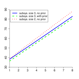
(a)

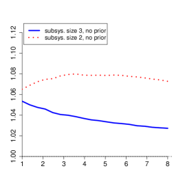
(b)

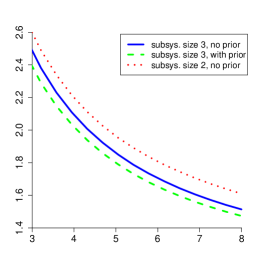
(c)

Figure 2: Performance of the tests under the first study, where $K=7$.

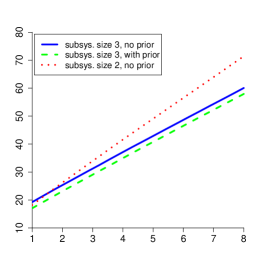
(a)

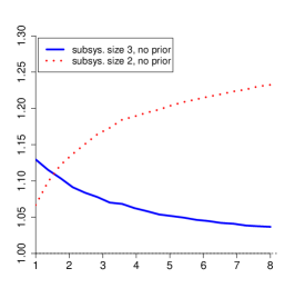
(b)

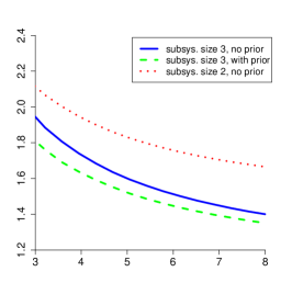
(c)

Figure 3: Performance of the tests under the second study, where $K=3$.

8 Conclusion

In the present paper we consider a setup where multiple data streams are generated by distinct data sources and we propose a novel multiple testing formulation that unifies the problems of detection and isolation. Specifically, we introduce a family of testing procedures, of various computational complexities, that control 4 distinct error metrics, two of which are related to the pure detection problem and two to the pure isolation problem. We characterize the optimal expected sample size in the class of all sequential tests that control these error probabilities to a first-order asymptotic approximation as the latter go to 0. Moreover, we evaluate the asymptotic relative efficiency of low-complexity rules in the proposed family, and establish sufficient conditions for their asymptotic optimality.

Unlike most previous works in the literature, the results in the present paper do not rely on the assumption of independence among the data sources. Thus, we apply them to the problem of detecting and isolating (i) anomalous, possibly dependent, data streams, (ii) an unknown dependence structure. For the first of these problems, in the case of independence we obtain asymptotically optimal rules that are easily implementable in practice, under general conditions that allow for temporal dependence. Thus, we generalize previous results in the literature, which focus either on the pure detection or the pure isolation problem.

There are various natural generalizations of the present work. For example, we can obtain a similar asymptotic theory using alternative metrics for the false positive and false negative rates, such as FDR, pFDR, etc., working similarly to [19]. Moreover, we can extend the results of the current work to the case that the distribution of each unit under each hypothesis belongs to a parametric family, working similarly to [35, Section 6].

Finally, there are many open questions and directions for further research, such as a more precise description of the optimal performance, the proof of stronger optimality properties, asymptotic regimes where the number of sources also goes to infinity as the error probabilities vanish, modeling the data streams using spatial models, e.g., a Markov random field, where the special underlying dependence can lead to further insights, closed-form expressions for the thresholds that are less conservative than the ones we obtain in this work, more efficient design of subsystems, etc. Finally, another direction of interest is to allow for the sampling to be terminated at a different time in each data stream, as in [4, 7, 29].

This work was supported in part by NSF Grant DMS-1737962.

Appendix A Proofs regarding Error Control

A.1 Some important lemmas

In this subsection we establish some lemmas which are critical in establishing the error control in Theorems 3.1 and 3.2.

Lemma A.1.

Suppose $\emptyset\in\Psi$. Fix any $e\in\mathcal{K}$ and $D_{e}>1$. If ${\sf P}\in\mathcal{H}_{0}$ then

$${\sf P}\left(\Lambda_{e,\rm det}\left(n\right)\geq D_{e}\ \;\;\text{for some}\ \;\;n\in\mathbb{N}\right)\leq\frac{|\mathcal{G}_{\Psi,e}^{s_{e}}|}{D_{e}}.$$

Proof.

We have,

$${\sf P}\left(\Lambda_{e,\rm det}\left(n\right)\geq D_{e}\ \;\;\text{for some}\ \;\;n\in\mathbb{N}\right)$$

$$={\sf P}^{s_{e}}\left(\Lambda_{e,\rm det}\left(n\right)\geq D_{e}\ \;\;\text{for some}\ \;\;n\in\mathbb{N}\right)$$

$$\leq{\sf P}^{s_{e}}\left(\max_{{\sf Q}\in\mathcal{G}_{\Psi,e}^{s_{e}}}\frac{\Lambda_{n}({\sf Q},{\sf P}_{0})}{\Lambda_{n}({\sf P}^{s_{e}},{\sf P}_{0})}\geq D_{e}\ \;\;\text{for some}\ \;\;n\in\mathbb{N}\right),\ \text{since}\ \;\;{\sf P}^{s_{e}}\in\mathcal{H}_{0}^{s_{e}}$$

$$\leq{\sf P}^{s_{e}}\left(\bigcup_{{\sf Q}\in\mathcal{G}_{\Psi,e}^{s_{e}}}\left\{\frac{\Lambda_{n}({\sf Q},{\sf P}_{0})}{\Lambda_{n}({\sf P}^{s_{e}},{\sf P}_{0})}\geq D_{e}\ \;\;\text{for some}\ \;\;n\in\mathbb{N}\right\}\right)$$

$$\leq\sum_{{\sf Q}\in\mathcal{G}_{\Psi,e}^{s_{e}}}{\sf P}^{s_{e}}\left(\Lambda_{n}({\sf Q},{\sf P}^{s_{e}})\geq D_{e}\ \;\;\text{for some}\ \;\;n\in\mathbb{N}\right)$$

$$\leq\sum_{{\sf Q}\in\mathcal{G}_{\Psi,e}^{s_{e}}}\frac{1}{D_{e}}=\frac{|\mathcal{G}_{\Psi,e}^{s_{e}}|}{D_{e}},$$

where the third inequality follows from Boole’s inequality and the last one follows from Ville’s inequality. ∎

Lemma A.2.

Suppose $\emptyset\in\Psi$. Fix any ${\sf P}\in\mathcal{P}_{\Psi}\setminus\mathcal{H}_{0}$, $e\in\mathcal{A}({\sf P})$ and $C_{e}>1$. Then

$${\sf P}\left(\Lambda_{e,\rm det}\left(n\right)\leq\frac{1}{C_{e}}\ \;\;\text{for some}\ \;\;n\in\mathbb{N}\right)\leq\frac{|\mathcal{H}_{0}^{s_{e}}|}{C_{e}}.$$

Proof.

Since $e\in\mathcal{A}({\sf P})$ and ${\sf P}\in\mathcal{P}_{\Psi}\setminus\mathcal{H}_{0}$, we have ${\sf P}\in\mathcal{G}_{\Psi,e}$. Now,

$${\sf P}\left(\Lambda_{e,\rm det}\left(n\right)\leq\frac{1}{C_{e}}\ \;\;\text{for some}\ \;\;n\in\mathbb{N}\right)$$

$$={\sf P}^{s_{e}}\left(\Lambda_{e,\rm det}\left(n\right)\leq\frac{1}{C_{e}}\ \;\;\text{for some}\ \;\;n\in\mathbb{N}\right)$$

$$\leq{\sf P}^{s_{e}}\left(\max_{{\sf Q}\in\mathcal{H}_{0}^{s_{e}}}\frac{\Lambda_{n}({\sf Q},{\sf P}_{0})}{\Lambda_{n}({\sf P}^{s_{e}},{\sf P}_{0})}\geq C_{e}\ \;\;\text{for some}\ \;\;n\in\mathbb{N}\right),\ \text{since}\ \;\;{\sf P}^{s_{e}}\in\mathcal{G}_{\Psi,e}^{s_{e}}$$

$$\leq{\sf P}^{s_{e}}\left(\bigcup_{{\sf Q}\in\mathcal{H}_{0}^{s_{e}}}\left\{\frac{\Lambda_{n}({\sf Q},{\sf P}_{0})}{\Lambda_{n}({\sf P}^{s_{e}},{\sf P}_{0})}\geq C_{e}\ \;\;\text{for some}\ \;\;n\in\mathbb{N}\right\}\right)$$

$$\leq\sum_{{\sf Q}\in\mathcal{H}_{0}^{s_{e}}}{\sf P}^{s_{e}}\left(\Lambda_{n}({\sf Q},{\sf P}^{s_{e}})\geq C_{e}\ \;\;\text{for some}\ \;\;n\in\mathbb{N}\right)$$

$$\leq\sum_{{\sf Q}\in\mathcal{H}_{0}^{s_{e}}}\frac{1}{C_{e}}=\frac{|\mathcal{H}_{0}^{s_{e}}|}{C_{e}},$$

where the third inequality follows from Boole’s inequality and the last one follows from Ville’s inequality. ∎

Lemma A.3.

Suppose $\emptyset\in\Psi$. Fix any ${\sf P}\in\mathcal{P}_{\Psi}\setminus\mathcal{H}_{0}$, $e\notin\mathcal{A}({\sf P})$ and $B_{e}>1$. Then

$${\sf P}\left(\Lambda_{e,\rm iso}\left(n\right)\geq B_{e}\ \;\;\text{for some}\ \;\;n\in\mathbb{N}\right)\leq\frac{|\mathcal{G}_{\Psi,e}^{s^{\prime}_{e}}|}{B_{e}}.$$

Proof.

Since $e\notin\mathcal{A}({\sf P})$ and ${\sf P}\in\mathcal{P}_{\Psi}\setminus\mathcal{H}_{0}$, we have ${\sf P}\in\mathcal{H}_{\Psi,e}$. Now,

$${\sf P}\left(\Lambda_{e,\rm iso}\left(n\right)\geq B_{e}\ \;\;\text{for some}\ \;\;n\in\mathbb{N}\right)$$

$$={\sf P}^{s^{\prime}_{e}}\left(\Lambda_{e,\rm iso}\left(n\right)\geq B_{e}\ \;\;\text{for some}\ \;\;n\in\mathbb{N}\right)$$

$$\leq{\sf P}^{s^{\prime}_{e}}\left(\max_{{\sf Q}\in\mathcal{G}_{\Psi,e}^{s^{\prime}_{e}}}\frac{\Lambda_{n}({\sf Q},{\sf P}_{0})}{\Lambda_{n}({\sf P}^{s^{\prime}_{e}},{\sf P}_{0})}\geq B_{e}\ \;\;\text{for some}\ \;\;n\in\mathbb{N}\right),\ \text{since}\ \;\;{\sf P}^{s^{\prime}_{e}}\in\mathcal{H}_{\Psi,e}^{s^{\prime}_{e}}$$

$$\leq{\sf P}^{s^{\prime}_{e}}\left(\bigcup_{{\sf Q}\in\mathcal{G}_{\Psi,e}^{s^{\prime}_{e}}}\left\{\frac{\Lambda_{n}({\sf Q},{\sf P}_{0})}{\Lambda_{n}({\sf P}^{s^{\prime}_{e}},{\sf P}_{0})}\geq B_{e}\ \;\;\text{for some}\ \;\;n\in\mathbb{N}\right\}\right)$$

$$\leq\sum_{{\sf Q}\in\mathcal{G}_{\Psi,e}^{s^{\prime}_{e}}}{\sf P}^{s^{\prime}_{e}}\left(\Lambda_{n}({\sf Q},{\sf P}^{s^{\prime}_{e}})\geq B_{e}\ \;\;\text{for some}\ \;\;n\in\mathbb{N}\right)$$

$$\leq\sum_{{\sf Q}\in\mathcal{G}_{\Psi,e}^{s^{\prime}_{e}}}\frac{1}{B_{e}}=\frac{|\mathcal{G}_{\Psi,e}^{s^{\prime}_{e}}|}{B_{e}},$$

where the third inequality follows from Boole’s inequality and the last one follows from Ville’s inequality. ∎

Lemma A.4.

Suppose $\emptyset\in\Psi$. Fix any ${\sf P}\in\mathcal{P}_{\Psi}\setminus\mathcal{H}_{0}$, $e\in\mathcal{A}({\sf P})$ and $A_{e}>1$. Then

$${\sf P}\left(\Lambda_{e,\rm iso}\left(n\right)\leq\frac{1}{A_{e}}\ \;\;\text{for some}\ \;\;n\in\mathbb{N}\right)\leq\frac{|\mathcal{H}_{\Psi,e}^{s^{\prime}_{e}}|}{A_{e}}.$$

Proof.

Since $e\in\mathcal{A}({\sf P})$ and ${\sf P}\in\mathcal{P}_{\Psi}\setminus\mathcal{H}_{0}$, we have ${\sf P}\in\mathcal{G}_{\Psi,e}$. Now,

$${\sf P}\left(\Lambda_{e,\rm iso}\left(n\right)\leq\frac{1}{A_{e}}\ \;\;\text{for some}\ \;\;n\in\mathbb{N}\right)$$

$$={\sf P}^{s^{\prime}_{e}}\left(\Lambda_{e,\rm iso}\left(n\right)\leq\frac{1}{A_{e}}\ \;\;\text{for some}\ \;\;n\in\mathbb{N}\right)$$

$$\leq{\sf P}^{s^{\prime}_{e}}\left(\max_{{\sf Q}\in\mathcal{H}_{\Psi,e}^{s^{\prime}_{e}}}\frac{\Lambda_{n}({\sf Q},{\sf P}_{0})}{\Lambda_{n}({\sf P}^{s^{\prime}_{e}},{\sf P}_{0})}\geq A_{e}\ \;\;\text{for some}\ \;\;n\in\mathbb{N}\right),\ \text{since}\ \;\;{\sf P}^{s^{\prime}_{e}}\in\mathcal{G}_{\Psi,e}^{s^{\prime}_{e}}$$

$$\leq{\sf P}^{s^{\prime}_{e}}\left(\bigcup_{{\sf Q}\in\mathcal{H}_{\Psi,e}^{s^{\prime}_{e}}}\left\{\frac{\Lambda_{n}({\sf Q},{\sf P}_{0})}{\Lambda_{n}({\sf P}^{s^{\prime}_{e}},{\sf P}_{0})}\geq A_{e}\ \;\;\text{for some}\ \;\;n\in\mathbb{N}\right\}\right)$$

$$\leq\sum_{{\sf Q}\in\mathcal{H}_{\Psi,e}^{s^{\prime}_{e}}}{\sf P}^{s^{\prime}_{e}}\left(\Lambda_{n}({\sf Q},{\sf P}^{s^{\prime}_{e}})\geq A_{e}\ \;\;\text{for some}\ \;\;n\in\mathbb{N}\right)$$

$$\leq\sum_{{\sf Q}\in\mathcal{H}_{\Psi,e}^{s^{\prime}_{e}}}\frac{1}{A_{e}}=\frac{|\mathcal{H}_{\Psi,e}^{s^{\prime}_{e}}|}{A_{e}},$$

where the third inequality follows from Boole’s inequality and the last one follows from Ville’s inequality. ∎

A.2 Proof of Theorem 3.1

Proof.

The first part of the proof is similar to the proof of Theorem 3.2(iii), which is done later.

For the second part, note that when $\Psi=\Psi_{m,m}$ for some $0<m<|\mathcal{K}|$, then for any $(T,D)\in\mathcal{C}_{\Psi}(\gamma,\delta)$, we have ${\sf P}\left(D\setminus\mathcal{A}({\sf P})\neq\emptyset\right)={\sf P}\left(\mathcal{A}({\sf P})\setminus D\neq\emptyset\right)={\sf P}\left(D\neq\mathcal{A}({\sf P})\right)\leq\gamma\wedge\delta$. Therefore, replacing both $\gamma$ and $\delta$ by $\gamma\wedge\delta$ in the lower bounds of $A_{e}$ and $B_{e}$ gives us the result. ∎

A.3 Proof of Theorem 3.2

Proof.

First, we prove (iii) since the proof of (i) follows similarly. Fix the thresholds $\{A_{e},B_{e},C_{e},D_{e}\}_{e\in\mathcal{K}}>1$. We detect that there is at least one unit in which alternative is correct only when $T_{joint}<T_{0}$ which means $\left\{\Lambda_{e,\rm det}\left(T^{*}\right)\geq D_{e}\right\}$ for some $e\in\mathcal{K}$. Formally,

$$\left\{D^{*}\neq\emptyset\right\}\subseteq\bigcup_{e\in\mathcal{K}}\left\{\Lambda_{e,\rm det}\left(T^{*}\right)\geq D_{e}\right\}.$$

Now, consider any arbitrary ${\sf P}\in\mathcal{H}_{0}$. Then, we have

$${\sf P}\left(D^{*}\neq\emptyset\right) \leq\sum_{e\in\mathcal{K}}{\sf P}\left(\Lambda_{e,\rm det}\left(T^{*}\right)\geq D_{e}\right)$$

$$\leq\sum_{e\in\mathcal{K}}{\sf P}\left(\Lambda_{e,\rm det}\left(n\right)\geq D_{e}\ \;\;\text{for some}\ \;\;n\in\mathbb{N}\right)$$

$$\leq\sum_{e\in\mathcal{K}}\frac{|\mathcal{G}_{\Psi,e}^{s_{e}}|}{D_{e}}$$

where the first inequality follows from Boole’s inequality and the third one follows from Lemma A.1. Thus, if we select $D_{e}$ according to (i), the probability of false alarm is controlled.

For the rest of the proof of (iii), consider any arbitrary ${\sf P}\in\mathcal{P}_{\Psi}\setminus\mathcal{H}_{0}$. We detect that null hypothesis is true in all units only if $T_{0}<T_{joint}$, which means $\left\{\Lambda_{e,\rm det}\left(T^{*}\right)\leq\frac{1}{C_{e}}\right\}$ for all $e\in\mathcal{K}$, and therefore, for any arbitrary $e\in\mathcal{A}({\sf P})$. Formally,

$$\left\{D^{*}=\emptyset\right\}\subseteq\left\{\Lambda_{e,\rm det}\left(T^{*}\right)\leq\frac{1}{C_{e}}\right\},$$

which implies

$${\sf P}\left(D^{*}=\emptyset\right) \leq{\sf P}\left(\Lambda_{e,\rm det}\left(T^{*}\right)\leq\frac{1}{C_{e}}\right)$$

$$\leq{\sf P}\left(\Lambda_{e,\rm det}\left(n\right)\leq\frac{1}{C_{e}}\ \;\;\text{for some}\ \;\;n\in\mathbb{N}\right)$$

$$\leq\frac{|\mathcal{H}_{0}^{s_{e}}|}{C_{e}},$$

where the third inequality follows from Lemma A.2. Thus, if we select $C_{e}$ according to (i), the probability of missed detection is controlled.

Note that, at least one false positive is made only if $T_{joint}<T_{0}$ and we mistakenly isolate a unit in which null is true. Formally, the event $\left\{\Lambda_{e,\rm iso}(T^{*})\geq B_{e}\right\}$ happens for some $e\notin\mathcal{A}({\sf P})$, i.e.,

$$\left\{D^{*}\setminus\mathcal{A}({\sf P})\neq\emptyset\right\}\subseteq\bigcup_{e\notin\mathcal{A}({\sf P})}\left\{\Lambda_{e,\rm iso}(T^{*})\geq B_{e}\right\},$$

which implies

$${\sf P}\left(D^{*}\setminus\mathcal{A}({\sf P})\neq\emptyset\right) \leq\sum_{e\notin\mathcal{A}({\sf P})}{\sf P}\left(\Lambda_{e,\rm iso}\left(T^{*}\right)\geq B_{e}\right)$$

$$\leq\sum_{e\notin\mathcal{A}({\sf P})}{\sf P}\left(\Lambda_{e,\rm iso}\left(n\right)\geq B_{e}\ \;\;\text{for some}\ \;\;n\in\mathbb{N}\right)$$

$$\leq\sum_{e\notin\mathcal{A}({\sf P})}\frac{|\mathcal{G}_{\Psi,e}^{s^{\prime}_{e}}|}{B_{e}}\leq\sum_{e\in\mathcal{K}}\frac{|\mathcal{G}_{\Psi,e}^{s^{\prime}_{e}}|}{B_{e}},$$

where the first inequality follows from Boole’s inequality and the third one follows from Lemma A.3. Thus, if we select $B_{e}$ as in Theorem 3.1 we obtain the desired error control.

Next, observe that at least one false negative is made and $D^{*}\neq\emptyset$ only if $T_{joint}<T_{0}$ and we fail to isolate a unit in which alternative is true. Formally, the event $\left\{\Lambda_{e,\rm iso}(T^{*})\leq\frac{1}{A_{e}}\right\}$ happens for some $e\in\mathcal{A}({\sf P})$, i.e.,

$$\left\{\mathcal{A}({\sf P})\setminus D^{*}\neq\emptyset,D^{*}\neq\emptyset\right\}\subseteq\bigcup_{e\in\mathcal{A}({\sf P})}\left\{\Lambda_{e,\rm iso}(T^{*})\leq\frac{1}{A_{e}}\right\},$$

which implies,

$${\sf P}\left(\mathcal{A}({\sf P})\setminus D^{*}\neq\emptyset,D^{*}\neq\emptyset\right) \leq\sum_{e\in\mathcal{A}({\sf P})}{\sf P}\left(\Lambda_{e,\rm iso}\left(T^{*}\right)\leq\frac{1}{A_{e}}\right)$$

$$\leq\sum_{e\in\mathcal{A}({\sf P})}{\sf P}\left(\Lambda_{e,\rm iso}\left(n\right)\leq\frac{1}{A_{e}}\ \;\;\text{for some}\ \;\;n\in\mathbb{N}\right)$$

$$\leq\sum_{e\in\mathcal{A}({\sf P})}\frac{|\mathcal{H}_{\Psi,e}^{s^{\prime}_{e}}|}{A_{e}}\leq\sum_{e\in\mathcal{K}}\frac{|\mathcal{H}_{\Psi,e}^{s^{\prime}_{e}}|}{A_{e}}$$

where the first inequality follows from Boole’s inequality and the third one follows from Lemma A.4. Thus, if we select $A_{e}$ as in Theorem 3.1 we obtain the desired error control.

Next, we prove (ii) regarding $\chi^{*}_{fwer}$, where the thresholds in $\chi^{*}$ are selected such that $A_{e}=C_{e}$ and $B_{e}=D_{e}$ for every $e\in\mathcal{K}$. Fix any arbitrary ${\sf P}\in\mathcal{P}_{\Psi}$. Note that, at least one false positive is made if there exists some $e\in D^{*}_{fwer}\setminus\mathcal{A}({\sf P})$. Now, $e\notin\mathcal{A}({\sf P})$ means either ${\sf P}\in\mathcal{H}_{0}$ or ${\sf P}\in\mathcal{H}_{\Psi,e}$. Suppose the first case holds, that is, ${\sf P}\in\mathcal{H}_{0}$. Then,

$${\sf P}\left(D^{*}_{fwer}\setminus\mathcal{A}({\sf P})\neq\emptyset\right) ={\sf P}\left(D^{*}_{fwer}\neq\emptyset\right)$$

$$\leq\sum_{e\in\mathcal{K}}{\sf P}\left(\Lambda_{e,\rm det}\left(T^{*}_{fwer}\right)\geq B_{e}\right)$$

$$\leq\sum_{e\in\mathcal{K}}{\sf P}\left(\Lambda_{e,\rm det}\left(n\right)\geq B_{e}\ \;\;\text{for some}\ \;\;n\in\mathbb{N}\right)$$

$$\leq\sum_{e\in\mathcal{K}}\frac{|\mathcal{G}_{\Psi,e}^{s_{e}}|}{B_{e}}$$ (25)

where the first inequality follows from Boole’s inequality and the third one follows from Lemma A.1. If the second case holds, that is, ${\sf P}\in\mathcal{H}_{\Psi,e}$, then

$${\sf P}\left(D^{*}_{fwer}\setminus\mathcal{A}({\sf P})\neq\emptyset\right) \leq\sum_{e\notin\mathcal{A}({\sf P})}{\sf P}\left(\Lambda_{e,\rm iso}(T^{*}_{fwer})\geq B_{e}\right)$$

$$\leq\sum_{e\notin\mathcal{A}({\sf P})}{\sf P}\left(\Lambda_{e,\rm iso}\left(n\right)\geq B_{e}\ \;\;\text{for some}\ \;\;n\in\mathbb{N}\right)$$

$$\leq\sum_{e\notin\mathcal{A}({\sf P})}\frac{|\mathcal{G}_{\Psi,e}^{s^{\prime}_{e}}|}{B_{e}}\leq\sum_{e\in\mathcal{K}}\frac{|\mathcal{G}_{\Psi,e}^{s^{\prime}_{e}}|}{B_{e}},$$ (26)

where the first inequality follows from Boole’s inequality and the third one follows from Lemma A.3. Then, from (25) and (26), we have

$${\sf P}\left(D^{*}_{fwer}\setminus\mathcal{A}({\sf P})\neq\emptyset\right)\leq\sum_{e\in\mathcal{K}}\frac{|\mathcal{G}_{\Psi,e}^{s_{e}}|\vee|\mathcal{G}_{\Psi,e}^{s^{\prime}_{e}}|}{B_{e}}.$$

Thus, if we select $B_{e}$ according to (ii), we obtain the desired error control.

Next, observe that at least one false negative is made if either $T_{0}<T_{joint}$ and we simply declare $D^{*}_{fwer}=\emptyset$, or $T_{joint}<T_{0}$ and we incur the event $\{\mathcal{A}({\sf P})\setminus D^{*}_{fwer}\neq\emptyset,D^{*}_{fwer}\neq\emptyset\}$. Formally,

$$\{\mathcal{A}({\sf P})\setminus D^{*}_{fwer}\neq\emptyset\}=\{D^{*}_{fwer}=\emptyset\}\cup\{\mathcal{A}({\sf P})\setminus D^{*}_{fwer}\neq\emptyset,D^{*}_{fwer}\neq\emptyset\}.$$

For any $e\in\mathcal{A}({\sf P})$, the probability of the first event can be bounded as follows:

$${\sf P}\left(D^{*}_{fwer}=\emptyset\right) \leq{\sf P}\left(\Lambda_{e,\rm det}\left(T^{*}_{fwer}\right)\leq\frac{1}{A_{e}}\right)$$

$$\leq{\sf P}\left(\Lambda_{e,\rm det}\left(n\right)\leq\frac{1}{A_{e}}\ \;\;\text{for some}\ \;\;n\in\mathbb{N}\right)$$

$$\leq\frac{|\mathcal{H}_{0}^{s_{e}}|}{A_{e}},$$ (27)

where the third inequality follows from Lemma A.2. Furthermore, for the second event, we have

$${\sf P}\left(\mathcal{A}({\sf P})\setminus D^{*}_{fwer}\neq\emptyset,D^{*}_{fwer}\neq\emptyset\right) \leq\sum_{e\in\mathcal{A}({\sf P})}{\sf P}\left(\Lambda_{e,\rm iso}\left(T^{*}_{fwer}\right)\leq\frac{1}{A_{e}}\right)$$

$$\leq\sum_{e\in\mathcal{A}({\sf P})}{\sf P}\left(\Lambda_{e,\rm iso}\left(n\right)\leq\frac{1}{A_{e}}\ \;\;\text{for some}\ \;\;n\in\mathbb{N}\right)$$

$$\leq\sum_{e\in\mathcal{A}({\sf P})}\frac{|\mathcal{H}_{\Psi,e}^{s^{\prime}_{e}}|}{A_{e}}\leq\sum_{e\in\mathcal{K}}\frac{|\mathcal{H}_{\Psi,e}^{s^{\prime}_{e}}|}{A_{e}},$$ (28)

where the third inequality follows from Lemma A.4. Then from (27) and (28), we have

$${\sf P}\left(\mathcal{A}({\sf P})\setminus D^{*}_{fwer}\neq\emptyset\right) \leq\frac{|\mathcal{H}_{0}^{s_{e}}|}{A_{e}}+\sum_{e\in\mathcal{K}}\frac{|\mathcal{H}_{\Psi,e}^{s^{\prime}_{e}}|}{A_{e}}$$

$$\leq\frac{|\mathcal{H}_{0}^{s_{e}}|\vee|\mathcal{H}_{\Psi,e}^{s^{\prime}_{e}}|}{A_{e}}+\sum_{e\in\mathcal{K}}\frac{|\mathcal{H}_{0}^{s_{e}}|\vee|\mathcal{H}_{\Psi,e}^{s^{\prime}_{e}}|}{A_{e}}.$$

Thus, if we select $A_{e}$ according to (ii), we obtain the desired error control.

Further, note that, for any $e\in\mathcal{K}$ if $s_{e}=s^{\prime}_{e}=e$ then $b_{e}=d_{e}=|\mathcal{G}^{e}|$, and $a_{e}=c_{e}=|\mathcal{H}^{e}|$. Thus, $B_{e}\geq(b_{e}\vee d_{e})|\mathcal{K}|/\gamma=b_{e}|\mathcal{K}|/\gamma$. On the other hand, one can bound the probability of at least one false negative as follows.

$${\sf P}\left(\mathcal{A}({\sf P})\setminus D^{*}_{fwer}\neq\emptyset\right) \leq\sum_{e\in\mathcal{A}({\sf P})}{\sf P}\left(\Lambda_{e}(T^{*}_{fwer})\leq\frac{1}{A_{e}}\right)$$

$$\leq\sum_{e\in\mathcal{A}({\sf P})}{\sf P}\left(\Lambda_{e}(n)\leq\frac{1}{A_{e}}\ \;\;\text{for some}\ \;\;n\in\mathbb{N}\right)$$

$$\leq\sum_{e\in\mathcal{A}({\sf P})}\frac{|\mathcal{H}^{e}|}{A_{e}}\leq\sum_{e\in\mathcal{K}}\frac{a_{e}}{A_{e}}$$

where the first inequality follows from Boole’s inequality and the last one follows form Lemma A.4. Thus, if we select $A_{e}$ according to (ii), we obtain the desired error control. The proof is complete. ∎

Appendix B Some properties regarding the Information Numbers

In this section, we present some important lemmas about the information numbers introduced in Section 4, which are critical to establishing Proposition D.1 in Appendix D as well as may be of independent interest to the reader.

Lemma B.1.

Suppose that (11) holds for two distinct probability distributions ${\sf P},{\sf Q}\in\mathcal{P}$, when $s=s_{1},s_{2}\subseteq[K]$.

$$\text{If}\quad s_{1}\subseteq s_{2},\quad\text{then}\quad\mathcal{I}({\sf P},{\sf Q};s_{1})\leq\mathcal{I}\left({\sf P},{\sf Q};s_{2}\right).$$

Proof.

Consider the hypotheses testing problem

$$H_{0}:X\sim{\sf P}\quad\text{versus}\quad H_{1}:X\sim{\sf Q},$$

where we control both type 1 error and type 2 error below $\alpha$, for some $\alpha\in(0,1)$. A test, in this context, is a pair $(T,d)$ that consists of an $\{\mathcal{F}_{n}\}$-stopping time $T$ that represents the time at which the decision is taken and an $\mathcal{F}_{T}$-measurable bernoulli random variable $d$, such that $\{d=i\}$ represents hypothesis $H_{i}$ is selected upon stopping, $i=0,1$. Let $\mathcal{C}^{s}$ be the class of sequential procedures $(T,d)$ which satisfy the desired error control based on $\mathcal{F}^{s}$, that is, observations only from $s$. Since $s_{1}\subseteq s_{2}$, we have $\mathcal{F}_{n}^{s_{1}}\subseteq\mathcal{F}_{n}^{s_{2}}$ for every $n\in\mathbb{N}$, which implies $\mathcal{F}^{s_{1}}\subseteq\mathcal{F}^{s_{2}}$ and therefore, $\mathcal{C}^{s_{1}}\subseteq\mathcal{C}^{s_{2}}$. This leads to

$$\inf_{(T,d)\in\mathcal{C}^{s_{1}}}{\sf E}_{\sf P}\left[T\right]\geq\inf_{(T,d)\in\mathcal{C}^{s_{2}}}{\sf E}_{\sf P}\left[T\right].$$ (29)

Now, from [37, Lemma 3.4.1], as $\alpha\to 0$, we have

$$\inf_{(T,d)\in\mathcal{C}^{s}}{\sf E}_{\sf P}\left[T\right]\sim\frac{|\log\alpha|}{\mathcal{I}\left({\sf P},{\sf Q};s\right)},\quad s=s_{1},s_{2},$$

which combining with (29) completes the proof. ∎

Lemma B.2.

Consider ${\sf P}\in\mathcal{P}$ and class of probability distributions $\mathcal{Q}\subset\mathcal{P}$, where ${\sf P}\notin\mathcal{Q}$. Suppose that (11) holds for ${\sf P}$ and every ${\sf Q}\in\mathcal{Q}$, when $s=s_{1},s_{2}\subseteq[K]$.

$$\text{If}\quad s_{1}\subseteq s_{2},\quad\text{then}\quad\mathcal{I}({\sf P},\mathcal{Q};s_{1})\leq\mathcal{I}\left({\sf P},\mathcal{Q};s_{2}\right).$$

Proof.

From Lemma B.1, for every ${\sf Q}\in\mathcal{Q}$, we have

$$\mathcal{I}({\sf P},{\sf Q};s_{1})\leq\mathcal{I}({\sf P},{\sf Q};s_{2}).$$

Therefore, taking minimum over the class $\mathcal{Q}$ on both sides, we obtain

$$\mathcal{I}\left({\sf P},\mathcal{Q};s_{1}\right)=\min_{{\sf Q}\in\mathcal{Q}}\mathcal{I}\left({\sf P},{\sf Q};s_{1}\right)\leq\min_{{\sf Q}\in\mathcal{Q}}\mathcal{I}\left({\sf P},{\sf Q};s_{2}\right)=\mathcal{I}\left({\sf P},\mathcal{Q};s_{2}\right),$$

and the proof is complete. ∎

Lemma B.3.

Consider two disjoint subsets $s_{1},s_{2}\subset[K]$. Suppose that (11) and (12) hold for two distinct probability distribution ${\sf P},{\sf Q}\in\mathcal{P}$ when $s=s_{1},s_{2}$. If $s_{1}$ and $s_{2}$ are independent both under ${\sf P}$ and ${\sf Q}$, then (11) and (12) hold for ${\sf P}$, ${\sf Q}$ and $s=s_{1}\cup s_{2}$ with

$$\mathcal{I}({\sf P},{\sf Q};s)=\mathcal{I}\left({\sf P},{\sf Q};s_{1}\right)+\mathcal{I}\left({\sf P},{\sf Q};s_{2}\right).$$ (30)

Proof.

Let $s=s_{1}\cup s_{2}$. Since $s_{1}$ and $s_{2}$ are independent both under ${\sf P}$ and ${\sf Q}$, we have

$${\sf P}^{s}={\sf P}^{s_{1}}\otimes{\sf P}^{s_{2}},\quad\text{and}\quad{\sf Q}^{s}={\sf Q}^{s_{1}}\otimes{\sf Q}^{s_{2}}.$$

Now, suppose for a measurable set $A$, ${\sf Q}^{s}(A)=0$, which means

$${\sf Q}^{s_{1}}(A)\times{\sf Q}^{s_{2}}(A)=0$$

$$\Rightarrow\;\; {\sf Q}^{s_{1}}(A)=0\;\;\text{or},\;\;{\sf Q}^{s_{2}}(A)=0.$$

By the definition of absolute continuity, if the first case happens, then ${\sf P}^{s_{1}}(A)=0$, otherwise, ${\sf P}^{s_{2}}(A)=0$. Anyway, both cases lead to ${\sf P}^{s}(A)={\sf P}^{s_{1}}(A)\times{\sf P}^{s_{2}}(A)=0$. An exactly similar argument also shows that if ${\sf P}(A)=0$, then ${\sf Q}(A)=0$. Therefore, ${\sf P}$ and ${\sf Q}$ are mutually absolutely continuous when restricted to $\mathcal{F}_{n}^{s}$. Furthermore, we have the following decomposition of the likelihood process $\Lambda_{n}\left({\sf P}^{s},{\sf Q}^{s}\right)$:

$$\Lambda_{n}\left({\sf P}^{s},{\sf Q}^{s}\right)=\frac{d{\sf P}^{s_{1}}\otimes d{\sf P}^{s_{2}}}{d{\sf Q}^{s_{1}}\otimes d{\sf Q}^{s_{2}}}\left(\mathcal{F}_{n}^{s}\right) =\frac{d{\sf P}^{s_{1}}}{d{\sf Q}^{s_{1}}}\left(\mathcal{F}_{n}^{s_{1}}\right)\times\frac{d{\sf P}^{s_{2}}}{d{\sf Q}^{s_{2}}}\left(\mathcal{F}_{n}^{s_{2}}\right)$$

$$=\Lambda_{n}\left({\sf P}^{s_{1}},{\sf Q}^{s_{1}}\right)\times\Lambda_{n}\left({\sf P}^{s_{2}},{\sf Q}^{s_{2}}\right),$$

which subsequently leads us to

$$Z_{n}\left({\sf P}^{s},{\sf Q}^{s}\right)=Z_{n}\left({\sf P}^{s_{1}},{\sf Q}^{s_{1}}\right)+Z_{n}\left({\sf P}^{s_{2}},{\sf Q}^{s_{2}}\right).$$

Now, in order to prove (30), it suffices to show that

$${\sf P}\left(\max_{1\leq k\leq n}Z_{k}\left({\sf P}^{s},{\sf Q}^{s}\right)\geq n\rho\right)\to 0\quad\forall\,\rho>\mathcal{I}\left({\sf P},{\sf Q};s_{1}\right)+\mathcal{I}\left({\sf P},{\sf Q};s_{2}\right),$$ (31)

and at the same time

$$\sum_{n=1}^{\infty}{\sf P}\left(Z_{n}\left({\sf P}^{s},{\sf Q}^{s}\right)<n\rho\right)<\infty\quad\forall\,\rho<\mathcal{I}\left({\sf P},{\sf Q};s_{1}\right)+\mathcal{I}\left({\sf P},{\sf Q};s_{2}\right),$$ (32)

since these two conditions uniquely characterize the quantity $\mathcal{I}({\sf P},{\sf Q};s)$.

To start with, we fix an arbitrary $\rho>\mathcal{I}\left({\sf P},{\sf Q};s_{1}\right)+\mathcal{I}\left({\sf P},{\sf Q};s_{2}\right)$. Note that, there exist $\rho_{1}>\mathcal{I}\left({\sf P},{\sf Q};s_{1}\right)$ and $\rho_{2}>\mathcal{I}\left({\sf P},{\sf Q};s_{2}\right)$ such that $\rho=\rho_{1}+\rho_{2}$. Indeed, by letting $\delta=\rho-(\mathcal{I}\left({\sf P},{\sf Q};s_{1}\right)+\mathcal{I}\left({\sf P},{\sf Q};s_{2}\right))>0$, one can consider $\rho_{1}=\mathcal{I}\left({\sf P},{\sf Q};s_{1}\right)+\delta/2$ and $\rho_{2}=\mathcal{I}\left({\sf P},{\sf Q};s_{2}\right)+\delta/2$. Now,

$${\sf P}\left(\max_{1\leq k\leq n}Z_{k}\left({\sf P}^{s},{\sf Q}^{s}\right)\geq n\rho\right)$$

$$={\sf P}\left(\max_{1\leq k\leq n}\left\{Z_{k}\left({\sf P}^{s_{1}},{\sf Q}^{s_{1}}\right)+Z_{k}\left({\sf P}^{s_{2}},{\sf Q}^{s_{2}}\right)\right\}\geq n\rho\right)$$

$$\leq{\sf P}\left(\max_{1\leq k\leq n}Z_{k}\left({\sf P}^{s_{1}},{\sf Q}^{s_{1}}\right)+\max_{1\leq k\leq n}Z_{k}\left({\sf P}^{s_{2}},{\sf Q}^{s_{2}}\right)\geq n\rho_{1}+n\rho_{2}\right)$$

$$\leq{\sf P}\left(\max_{1\leq k\leq n}Z_{k}\left({\sf P}^{s_{1}},{\sf Q}^{s_{1}}\right)\geq n\rho_{1}\right)+{\sf P}\left(\max_{1\leq k\leq n}Z_{k}\left({\sf P}^{s_{2}},{\sf Q}^{s_{2}}\right)\geq n\rho_{2}\right),$$ (33)

where the first inequality follows from the fact that, for any two sequences $\{a_{n}\}_{n\in\mathbb{N}}$ and $\{b_{n}\}_{n\in\mathbb{N}}$,

$$\max_{1\leq k\leq n}\left\{a_{k}+b_{k}\right\}\leq\max_{1\leq k\leq n}a_{k}+\max_{1\leq k\leq n}b_{k},\quad\text{for every}\;\;n\in\mathbb{N},$$

and the last inequality is an application of Boole’s inequality. Since $\rho_{1}>\mathcal{I}\left({\sf P},{\sf Q};s_{1}\right)$ and $\rho_{2}>\mathcal{I}\left({\sf P},{\sf Q};s_{2}\right)$, due to condition (11), both the quantities on the right hand side of (33) converge to $0$ as $n\to\infty$. Hence, (31) follows.

In order to prove (32), we fix an arbitrary $\rho<\mathcal{I}\left({\sf P},{\sf Q};s_{1}\right)+\mathcal{I}\left({\sf P},{\sf Q};s_{2}\right)$. Note that, in a similar way like the previous, there exist $\rho_{1}<\mathcal{I}\left({\sf P},{\sf Q};s_{1}\right)$ and $\rho_{2}<\mathcal{I}\left({\sf P},{\sf Q};s_{2}\right)$ such that $\rho=\rho_{1}+\rho_{2}$. Now,

$$\sum_{n=1}^{\infty}{\sf P}\left(Z_{n}\left({\sf P}^{s},{\sf Q}^{s}\right)<n\rho\right)$$

$$=\sum_{n=1}^{\infty}{\sf P}\left(\left\{Z_{n}\left({\sf P}^{s_{1}},{\sf Q}^{s_{1}}\right)+Z_{n}\left({\sf P}^{s_{2}},{\sf Q}^{s_{2}}\right)\right\}<n\rho_{1}+n\rho_{2}\right)$$

$$\leq\sum_{n=1}^{\infty}{\sf P}\left(Z_{n}\left({\sf P}^{s_{1}},{\sf Q}^{s_{1}}\right)<n\rho_{1}\right)+{\sf P}\left(Z_{n}\left({\sf P}^{s_{2}},{\sf Q}^{s_{2}}\right)<n\rho_{2}\right)$$

$$=\sum_{n=1}^{\infty}{\sf P}\left(Z_{n}\left({\sf P}^{s_{1}},{\sf Q}^{s_{1}}\right)<n\rho_{1}\right)+\sum_{n=1}^{\infty}{\sf P}\left(Z_{n}\left({\sf P}^{s_{2}},{\sf Q}^{s_{2}}\right)<n\rho_{2}\right),$$ (34)

where the inequality follows from Boole’s inequality. Since $\rho_{1}<\mathcal{I}\left({\sf P},{\sf Q};s_{1}\right)$ and $\rho_{2}<\mathcal{I}\left({\sf P},{\sf Q};s_{2}\right)$, due to condition (12), both the quantities on the right hand side of (34) are finite. Hence, (32) follows and the proof is complete.

∎

Appendix C Proofs regarding Upper Bound on the expected sample size

In this section we only prove Theorem 4.2 since Theorem 4.1 can be established in a similar fashion.

C.1 Proof of Theorem 4.2

Proof.

It is sufficient to prove the results only for $\chi^{*}$ since it can be proved for the other tests in a similar way. Fix the thresholds $A_{e},B_{e},C_{e},D_{e}$ for all $e\in\mathcal{K}$ according to (8) and (9). Now for any ${\sf P}\in\mathcal{H}_{0}$, consider the stopping time

$$T_{\sf P}:=\inf\left\{n\geq 1:\min\left\{\Lambda_{n}\left({\sf P}^{s_{e}},{\sf Q}\right):{\sf Q}\in\mathcal{G}_{\Psi,e}^{s_{e}}\right\}\geq C_{e}\ \;\;\text{for every}\ \;\;e\in\mathcal{K}\right\}.$$

Under the assumption (12), from [36, Lemma F.2], it follows that as $\beta\to 0$,

$${\sf E}_{\sf P}\left[T_{\sf P}\right]\;\lesssim\;\max_{e\in\mathcal{K}}\left\{\frac{|\log\beta|}{\mathcal{I}\left({\sf P},\mathcal{G}_{\Psi,e};s_{e}\right)}\right\}.$$

Since $T^{*}\leq T_{0}$, it suffices to show that $T_{0}\leq T_{\sf P}$ for any given set of thresholds $\{C_{e}:e\in\mathcal{K}\}$. By the definition of $T_{0}$, it suffices to show that

$$\Lambda_{e,\rm det}(T_{\sf P})\leq\frac{1}{C_{e}}\ \;\;\text{for every}\ \;\;e\in\mathcal{K}.$$ (35)

To this end, fix any arbitrary $e\in\mathcal{K}$ and by the definition of $T_{\sf P}$, we have

$$\min\left\{\Lambda_{T_{\sf P}}\left({\sf P}^{s_{e}},{\sf Q}\right):{\sf Q}\in\mathcal{G}_{\Psi,e}^{s_{e}}\right\}\geq C_{e}.$$

As a result,

$$\frac{1}{C_{e}}\geq\max\left\{\Lambda_{T_{\sf P}}\left({\sf Q},{\sf P}^{s_{e}}\right):{\sf Q}\in\mathcal{G}_{\Psi,e}^{s_{e}}\right\} =\frac{\max\left\{\Lambda_{T_{\sf P}}\left({\sf Q},{\sf P}_{0}\right):{\sf Q}\in\mathcal{G}_{\Psi,e}^{s_{e}}\right\}}{\Lambda_{T_{\sf P}}\left({\sf P}^{s_{e}},{\sf P}_{0}\right)}$$

$$\geq\frac{\max\left\{\Lambda_{T_{\sf P}}\left({\sf Q},{\sf P}_{0}\right):{\sf Q}\in\mathcal{G}_{\Psi,e}^{s_{e}}\right\}}{\max\left\{\Lambda_{T_{\sf P}}\left({\sf Q},{\sf P}_{0}\right):{\sf Q}\in\mathcal{H}_{0}^{s_{e}}\right\}}$$

$$=\Lambda_{e,\rm det}(T_{\sf P}),$$

and the result follows in view of (35).

Now for any ${\sf P}\in\mathcal{P}_{\Psi}\setminus\mathcal{H}_{0}$, consider the stopping time

$$T^{\prime}_{\sf P}:=\inf\bigg{\{}n\geq 1: \min\left\{\Lambda_{n}\left({\sf P}^{s_{e}},{\sf Q}\right):{\sf Q}\in\mathcal{H}_{0}^{s_{e}}\right\}\geq D_{e}\ \;\;\text{for some}\ \;\;e\in\mathcal{A}({\sf P}),$$

$$\min\left\{\Lambda_{n}\left({\sf P}^{s^{\prime}_{e}},{\sf Q}\right):{\sf Q}\in\mathcal{H}_{\Psi,e}^{s^{\prime}_{e}}\right\}\geq B_{e}\ \;\;\text{for every}\ \;\;e\in\mathcal{A}({\sf P}),\quad\text{and}$$

$$\min\left\{\Lambda_{n}\left({\sf P}^{s^{\prime}_{e}},{\sf Q}\right):{\sf Q}\in\mathcal{G}_{\Psi,e}^{s^{\prime}_{e}}\right\}\geq A_{e}\ \;\;\text{for every}\ \;\;e\notin\mathcal{A}({\sf P})\bigg{\}}.$$

Under the assumption (12), from [36, Lemma F.2], it follows that as $\alpha,\gamma,\delta\to 0$,

$${\sf E}_{\sf P}\left[T^{\prime}_{{\sf P}}\right]\lesssim\min_{e\in\mathcal{A}({\sf P})}\left\{\frac{|\log\alpha|}{\mathcal{I}\left({\sf P},\mathcal{H}_{0};s_{e}\right)}\right\}\bigvee\max_{e\in\mathcal{A}({\sf P})}\left\{\frac{|\log\gamma|}{\mathcal{I}\left({\sf P},\mathcal{H}_{\Psi,e};s^{\prime}_{e}\right)}\right\}\bigvee\max_{e\notin\mathcal{A}({\sf P})}\left\{\frac{|\log\delta|}{\mathcal{I}\left({\sf P},\mathcal{G}_{\Psi,e};s^{\prime}_{e}\right)}\right\}.$$

Since $T^{*}\leq T_{joint}$, it suffices to show that $T_{joint}\leq T^{\prime}_{{\sf P}}$ for any given set of thresholds $\{A_{e},B_{e},D_{e}:e\in\mathcal{K}\}$. By the definition of $T_{joint}$ it suffices to show that

$$\begin{split}&\Lambda_{e,\rm det}\left(T^{\prime}_{\sf P}\right)\geq D_{e}\ \;\;\text{for some}\ \;\;e\in\mathcal{A}({\sf P}),\\ &\Lambda_{e,\rm iso}\left(T^{\prime}_{\sf P}\right)\geq B_{e}\ \;\;\text{for every}\ \;\;e\in\mathcal{A}({\sf P}),\\ &\Lambda_{e,\rm iso}\left(T^{\prime}_{\sf P}\right)\leq 1/A_{e}\ \;\;\text{for every}\ e\notin\mathcal{A}({\sf P}),\\ \text{and}\ \;\;&D_{\rm iso}\left(T^{\prime}_{\sf P}\right)\in\Psi.\end{split}$$ (36)

Now, note that if $e\in\mathcal{A}({\sf P})$, which means under ${\sf P}$ alternative is true in unit $e$, then ${\sf P}^{s}\in\mathcal{G}_{\Psi,e}^{s}$ for $s\in\{s_{e},s^{\prime}_{e}\}$.

To this end, consider that particular $e\in\mathcal{A}({\sf P})$ for which by definition of $T^{\prime}_{\sf P}$,

$$\min\left\{\Lambda_{T^{\prime}_{\sf P}}\left({\sf P}^{s_{e}},{\sf Q}\right):{\sf Q}\in\mathcal{H}_{0}^{s_{e}}\right\}\geq D_{e}.$$

As a result,

$$D_{e}\leq\min\left\{\Lambda_{T^{\prime}_{\sf P}}\left({\sf P}^{s_{e}},{\sf Q}\right):{\sf Q}\in\mathcal{H}_{0}^{s_{e}}\right\} =\frac{\Lambda_{T^{\prime}_{\sf P}}\left({\sf P}^{s_{e}},{\sf P}_{0}\right)}{\max\left\{\Lambda_{T^{\prime}_{\sf P}}\left({\sf Q},{\sf P}_{0}\right):{\sf Q}\in\mathcal{H}_{0}^{s_{e}}\right\}}$$

$$\leq\frac{\max\left\{\Lambda_{T^{\prime}_{\sf P}}\left({\sf Q},{\sf P}_{0}\right):{\sf Q}\in\mathcal{G}_{\Psi,e}^{s_{e}}\right\}}{\max\left\{\Lambda_{T^{\prime}_{\sf P}}\left({\sf Q},{\sf P}_{0}\right):{\sf Q}\in\mathcal{H}_{0}^{s_{e}}\right\}}=\Lambda_{e,\rm det}(T^{\prime}_{\sf P}),$$

where the last inequality follows because ${\sf P}\in\mathcal{G}_{\Psi,e}$.

Now fix any arbitrary $e\in\mathcal{A}({\sf P})$. Then by definition of $T^{\prime}_{\sf P}$, we have

$$\min\left\{\Lambda_{T^{\prime}_{\sf P}}\left({\sf P}^{s^{\prime}_{e}},{\sf Q}\right):{\sf Q}\in\mathcal{H}_{\Psi,e}^{s^{\prime}_{e}}\right\}\geq B_{e}.$$

As a result,

$$B_{e}\leq\min\left\{\Lambda_{T^{\prime}_{\sf P}}\left({\sf P}^{s^{\prime}_{e}},{\sf Q}\right):{\sf Q}\in\mathcal{H}_{\Psi,e}^{s^{\prime}_{e}}\right\} =\frac{\Lambda_{T^{\prime}_{\sf P}}\left({\sf P}^{s^{\prime}_{e}},{\sf P}_{0}\right)}{\max\left\{\Lambda_{T^{\prime}_{\sf P}}\left({\sf Q},{\sf P}_{0}\right):{\sf Q}\in\mathcal{H}_{\Psi,e}^{s^{\prime}_{e}}\right\}}$$

$$\leq\frac{\max\left\{\Lambda_{T^{\prime}_{\sf P}}\left({\sf Q},{\sf P}_{0}\right):{\sf Q}\in\mathcal{G}_{\Psi,e}^{s^{\prime}_{e}}\right\}}{\max\left\{\Lambda_{T^{\prime}_{\sf P}}\left({\sf Q},{\sf P}_{0}\right):{\sf Q}\in\mathcal{H}_{\Psi,e}^{s^{\prime}_{e}}\right\}}=\Lambda_{e,\rm iso}(T^{\prime}_{\sf P}),$$

where the last inequality follows because ${\sf P}\in\mathcal{G}_{\Psi,e}$.

Next, fix any arbitrary $e\notin\mathcal{A}({\sf P})$. Then by definition of $T^{\prime}_{\sf P}$, we have

$$\min\left\{\Lambda_{T^{\prime}_{\sf P}}\left({\sf P}^{s^{\prime}_{e}},{\sf Q}\right):{\sf Q}\in\mathcal{G}_{\Psi,e}^{s^{\prime}_{e}}\right\}\geq A_{e}.$$

As a result,

$$\frac{1}{A_{e}}\geq\max\left\{\Lambda_{T^{\prime}_{\sf P}}\left({\sf Q},{\sf P}^{s^{\prime}_{e}}\right):{\sf Q}\in\mathcal{G}_{\Psi,e}^{s^{\prime}_{e}}\right\} =\frac{\max\left\{\Lambda_{T^{\prime}_{\sf P}}\left({\sf Q},{\sf P}_{0}\right):{\sf Q}\in\mathcal{G}_{\Psi,e}^{s^{\prime}_{e}}\right\}}{\Lambda_{T^{\prime}_{\sf P}}\left({\sf P}^{s^{\prime}_{e}},{\sf P}_{0}\right)}$$

$$\geq\frac{\max\left\{\Lambda_{T^{\prime}_{\sf P}}\left({\sf Q},{\sf P}_{0}\right):{\sf Q}\in\mathcal{G}_{\Psi,e}^{s^{\prime}_{e}}\right\}}{\max\left\{\Lambda_{T^{\prime}_{\sf P}}\left({\sf Q},{\sf P}_{0}\right):{\sf Q}\in\mathcal{H}_{\Psi,e}^{s^{\prime}_{e}}\right\}}=\Lambda_{e,\rm iso}(T^{\prime}_{\sf P}),$$

where the last inequality follows because ${\sf P}\in\mathcal{H}_{\Psi,e}$. Therefore,

$$\Lambda_{e,\rm iso}(T^{\prime}_{\sf P})>1\quad\text{if and only if}\quad e\in\mathcal{A}({\sf P}),$$

which implies that $D_{\rm iso}(T^{\prime}_{{\sf P}})=\mathcal{A}({\sf P})\in\Psi$. Thus, the proof is complete in view of (36). ∎

Appendix D Proofs regarding Asymptotic Optimality

For any random variable $Y$ with underlying probability distribution ${\sf P}$ and any event $\Gamma$, we introduce the following notation:

$${\sf E}_{\sf P}\left[Y;\Gamma\right]:=\int_{\Gamma}Yd{\sf P},$$

which will be extensively used in this section.

D.1 Proof of Theorem 4.3

First, we establish a lemma which is critical in establishing an asymptotic lower bound on the optimal performance.

Lemma D.1.

Suppose that (11) holds, $\emptyset\notin\Psi$ and ${\sf P}\in\mathcal{P}_{\Psi}$. Then as $\gamma,\delta\to 0$ we have

$$\inf\left\{{\sf E}_{{\sf P}}[T]:\;(T,D)\in\mathcal{C}_{\Psi}(\gamma,\delta)\right\}\;\gtrsim\;\max_{e\in\mathcal{A}({\sf P})}\left\{\frac{|\log\gamma|}{\mathcal{I}({\sf P},\mathcal{H}_{\Psi,e})}\right\}\bigvee\max_{e\notin\mathcal{A}({\sf P})}\left\{\frac{|\log\delta|}{\mathcal{I}({\sf P},\mathcal{G}_{\Psi,e})}\right\}.$$

When in particular $\Psi=\Psi_{m,m}$ for some $0<m<|\mathcal{K}|$, then as $\gamma,\delta\to 0$ we have

$$\inf\left\{{\sf E}_{{\sf P}}[T]:\;(T,D)\in\mathcal{C}_{\Psi}(\gamma,\delta)\right\}\;\gtrsim\;\frac{|\log(\gamma\wedge\delta)|}{\mathcal{I}({\sf P},\mathcal{P}_{\Psi}\setminus\{{\sf P}\})}.$$

Proof.

Fix ${\sf P}\in\mathcal{P}_{\Psi}$ and denote the quantity $\inf\left\{{\sf E}_{{\sf P}}[T]:\;(T,D)\in\mathcal{C}_{\Psi}(\gamma,\delta)\right\}$ by $N(\gamma,\delta)$. Then we need to show that as $\gamma,\delta\to 0$,

$$N(\gamma,\delta)\gtrsim\max_{e\in\mathcal{A}({\sf P})}\left\{\frac{|\log\gamma|}{\mathcal{I}({\sf P},\mathcal{H}_{\Psi,e})}\right\}\bigvee\max_{e\notin\mathcal{A}({\sf P})}\left\{\frac{|\log\delta|}{\mathcal{I}({\sf P},\mathcal{G}_{\Psi,e})}\right\}.$$

We set

$$L_{\gamma}:=\max_{e\in\mathcal{A}({\sf P})}\left\{\frac{|\log\gamma|}{\mathcal{I}({\sf P},\mathcal{H}_{\Psi,e})}\right\},\quad\text{and}\quad L_{\delta}:=\max_{e\notin\mathcal{A}({\sf P})}\left\{\frac{|\log\delta|}{\mathcal{I}({\sf P},\mathcal{G}_{\Psi,e})}\right\}.$$

By Markov’s inequality, for any stopping time $T$ and $\gamma,\delta,\epsilon\in(0,1)$,

$${\sf E}_{\sf P}[T]\geq(1-\epsilon)L_{\gamma}{\sf P}\left(T\geq(1-\epsilon)L_{\gamma}\right)\quad\text{and}\quad{\sf E}_{\sf P}[T]\geq(1-\epsilon)L_{\delta}{\sf P}\left(T\geq(1-\epsilon)L_{\delta}\right).$$

Thus, it suffices to show for every $\epsilon\in(0,1)$ we have

$$\liminf_{\gamma,\delta\to 0}\inf_{(T,D)\in\mathcal{C}_{\Psi}(\gamma,\delta)}{\sf P}\left(T\geq(1-\epsilon)L_{\gamma}\right)\geq 1,\quad\text{and}$$ (37a)

$$\liminf_{\gamma,\delta\to 0}\inf_{(T,D)\in\mathcal{C}_{\Psi}(\gamma,\delta)}{\sf P}\left(T\geq(1-\epsilon)L_{\delta}\right)\geq 1,$$ (37b)

since this will further imply that

$$\liminf_{\gamma,\delta\to 0}\;N(\gamma,\delta)/(L_{\gamma}\vee L_{\delta})\geq(1-\epsilon),$$

and the desired result will follow by letting $\epsilon\to 0$. In order to prove (37), we start by fixing arbitrary $(T,D)\in\mathcal{C}_{\Psi}(\gamma,\delta)$ and $\gamma,\delta,\epsilon\in(0,1)$. To show (37a), consider the probability distribution ${\sf Q}_{1}^{*}$ which attains

$$\min\left\{\mathcal{I}({\sf P},{\sf Q}):{\sf Q}\in\cup_{e\in\mathcal{A}({\sf P})}\mathcal{H}_{\Psi,e}\right\}.$$

Thus, there exists $e\in\mathcal{A}({\sf P})$ such that ${\sf Q}_{1}^{*}\in\mathcal{H}_{\Psi,e}$, i.e., $e\notin\mathcal{A}({\sf Q}_{1}^{*})$. Then,

$${\sf P}\left(T\geq(1-\epsilon)L_{\gamma}\right) \geq{\sf P}\left(e\in D,T\geq(1-\epsilon)L_{\gamma}\right)$$

$$={\sf P}\left(e\in D\right)-{\sf P}\left(e\in D,T<(1-\epsilon)L_{\gamma}\right)$$

$$=1-{\sf P}\left(e\notin D\right)-{\sf P}\left(e\in D,T<(1-\epsilon)L_{\gamma}\right)$$

$$\geq 1-\delta-{\sf P}\left(e\in D,T<(1-\epsilon)L_{\gamma}\right)$$ (38)

where the last inequality follows from the fact that

$$\{e\notin D\}\subseteq\{\mathcal{A}({\sf P})\setminus D\neq\emptyset,D\neq\emptyset\}$$

and the error control that ${\sf P}\left(\mathcal{A}({\sf P})\setminus D\neq\emptyset,D\neq\emptyset\right)\leq\delta$. We can now decompose the third term as

$${\sf P}\left(e\in D,T<(1-\epsilon)L_{\gamma}\right)\leq p_{1}+p_{2},$$

such that

$$p_{1} :={\sf P}\left(e\in D,\Lambda_{T}({\sf P},{\sf Q}_{1}^{*})<\frac{\eta}{\gamma}\right)\quad\text{and}$$

$$p_{2} :={\sf P}\left(T<(1-\epsilon)L_{\gamma},\Lambda_{T}({\sf P},{\sf Q}_{1}^{*})\geq\frac{\eta}{\gamma}\right),$$

where $\eta$ is an arbitrary constant in $(0,1)$. For the first term, by a change of measure from ${\sf P}$ to ${\sf Q}_{1}^{*}$, we have

$$p_{1} ={\sf E}_{{\sf Q}_{1}^{*}}\left[\Lambda_{T}({\sf P},{\sf Q}_{1}^{*});e\in D,\Lambda_{T}({\sf P},{\sf Q}_{1}^{*})<\frac{\eta}{\gamma}\right]$$

$$\leq\frac{\eta}{\gamma}{\sf Q}_{1}^{*}\left(e\in D\right)\leq\eta,$$

where the last inequality follows from the fact that

$$\{e\in D\}\subseteq\{D\setminus\mathcal{A}({\sf Q}_{1}^{*})\neq\emptyset\}$$

and the error control that ${\sf Q}_{1}^{*}\left(D\setminus\mathcal{A}({\sf Q}_{1}^{*})\neq\emptyset\right)\leq\gamma$. For the second term,

$$p_{2}\leq{\sf P}\left(\frac{1}{(1-\epsilon)L_{\gamma}}\max_{1\leq n\leq(1-\epsilon)L_{\gamma}}\log\Lambda_{n}({\sf P},{\sf Q}_{1}^{*})\geq\frac{\log\eta}{(1-\epsilon)L_{\gamma}}+\frac{\mathcal{I}({\sf P},{\sf Q}_{1}^{*})}{(1-\epsilon)}\right)=:\xi_{\epsilon,\eta}(\gamma)$$

Due to (11), $\xi_{\epsilon,\eta}(\gamma)\to 0$ as $\gamma\to 0$.

Combining everything together in (38) we have

$${\sf P}(T\geq(1-\epsilon)L_{\gamma})\geq 1-\delta-\eta-\xi_{\epsilon,\eta}(\gamma).$$

Since $(T,D)\in\mathcal{C}_{\Psi}(\gamma,\delta)$ and $\gamma\in(0,1)$ were chosen arbitrarily, taking infimum over $(T,D)$ and letting $\gamma,\delta\to 0$ we obtain

$$\liminf_{\gamma,\delta\to 0}\inf_{(T,D)\in\mathcal{C}_{\Psi}(\gamma,\delta)}{\sf P}\left(T\geq(1-\epsilon)L_{\gamma}\right)\geq 1-\eta.$$

Finally, letting $\eta\to 0$ we obtain (37a).

To show (37b), consider the probability distribution ${\sf Q}_{2}^{*}$ which attains

$$\min\left\{\mathcal{I}({\sf P},{\sf Q}):{\sf Q}\in\cup_{e\notin\mathcal{A}({\sf P})}\mathcal{G}_{\Psi,e}\right\}.$$

Thus, there exists $e\notin\mathcal{A}({\sf P})$ such that ${\sf Q}_{2}^{*}\in\mathcal{G}_{\Psi,e}$, i.e., $e\in\mathcal{A}({\sf Q}_{2}^{*})$. Then,

$${\sf P}\left(T\geq(1-\epsilon)L_{\delta}\right) \geq{\sf P}\left(e\notin D,D\neq\emptyset,T\geq(1-\epsilon)L_{\delta}\right)$$

$$={\sf P}\left(e\notin D,D\neq\emptyset\right)-{\sf P}\left(e\notin D,D\neq\emptyset,T<(1-\epsilon)L_{\delta}\right)$$

$$=1-{\sf P}\left(e\in D,D\neq\emptyset\right)-{\sf P}\left(e\notin D,D\neq\emptyset,T<(1-\epsilon)L_{\delta}\right)$$

$$\geq 1-\gamma-{\sf P}\left(e\notin D,D\neq\emptyset,T<(1-\epsilon)L_{\delta}\right)$$ (39)

where the last inequality follows from the desired error control that ${\sf P}\left(D\setminus\mathcal{A}({\sf P})\neq\emptyset\right)\leq\gamma$. We can now decompose the third term as

$${\sf P}\left(e\notin D,D\neq\emptyset,T<(1-\epsilon)L_{\delta}\right)\leq p_{1}+p_{2},$$

such that

$$p_{1} :={\sf P}\left(e\notin D,D\neq\emptyset,\Lambda_{T}({\sf P},{\sf Q}_{2}^{*})<\frac{\eta}{\delta}\right)\quad\text{and}$$

$$p_{2} :={\sf P}\left(T<(1-\epsilon)L_{\delta},\Lambda_{T}({\sf P},{\sf Q}_{2}^{*})\geq\frac{\eta}{\delta}\right),$$

where $\eta$ is an arbitrary constant in $(0,1)$. For the first term, by a change of measure from ${\sf P}$ to ${\sf Q}_{2}^{*}$, we have

$$p_{1} ={\sf E}_{{\sf Q}_{2}^{*}}\left[\Lambda_{T}({\sf P},{\sf Q}_{2}^{*});e\notin D,D\neq\emptyset,\Lambda_{T}({\sf P},{\sf Q}_{2}^{*})<\frac{\eta}{\delta}\right]$$

$$\leq\frac{\eta}{\delta}{\sf Q}_{2}^{*}\left(e\notin D,D\neq\emptyset\right)\leq\eta,$$

where the last inequality follows from the desired error control that ${\sf Q}_{2}^{*}\left(\mathcal{A}({\sf Q}_{2}^{*})\setminus D\neq\emptyset,D\neq\emptyset\right)\leq\delta$. For the second term, we can bound it above by the similar manner as shown previously

$$p_{2}\leq{\sf P}\left(\frac{1}{(1-\epsilon)L_{\delta}}\max_{1\leq n\leq(1-\epsilon)L_{\delta}}\log\Lambda_{n}({\sf P},{\sf Q}_{2}^{*})\geq\frac{\log\eta}{(1-\epsilon)L_{\delta}}+\frac{\mathcal{I}({\sf P},{\sf Q}_{2}^{*})}{(1-\epsilon)}\right)=:\xi_{\epsilon,\eta}(\delta)$$

Due to (11), $\xi_{\epsilon,\eta}(\delta)\to 0$ as $\delta\to 0$.

Combining everything together in (39) we have

$${\sf P}(T\geq(1-\epsilon)L_{\delta})\geq 1-\gamma-\eta-\xi_{\epsilon,\eta}(\delta).$$

Since $(T,D)\in\mathcal{C}_{\Psi}(\gamma,\delta)$ and $\delta\in(0,1)$ were chosen arbitrarily, taking infimum over $(T,D)$ and letting $\gamma,\delta\to 0$ we obtain

$$\liminf_{\gamma,\delta\to 0}\inf_{(T,D)\in\mathcal{C}_{\Psi}(\gamma,\delta)}{\sf P}\left(T\geq(1-\epsilon)L_{\delta}\right)\geq 1-\eta.$$

Finally, letting $\eta\to 0$ we obtain (37b), which along with (37a) completes the first part of the proof.

For the second part, we first show that when $\Psi=\Psi_{m,m}$ we have

$$\cup_{e\in\mathcal{A}({\sf P})}\mathcal{H}_{\Psi,e}=\cup_{e\notin\mathcal{A}({\sf P})}\mathcal{G}_{\Psi,e}=\mathcal{P}_{\Psi}\setminus\{{\sf P}\}.$$

Indeed, the above holds since for any ${\sf Q}\in\mathcal{P}_{\Psi}\setminus\{{\sf P}\}$, as $|\mathcal{A}({\sf P})|=|\mathcal{A}({\sf Q})|=m$, there exists $e\in\mathcal{A}({\sf P})$ such that $e\notin\mathcal{A}({\sf Q})$, and also there exists $e\notin\mathcal{A}({\sf P})$ such that $e\in\mathcal{A}({\sf Q})$, i.e., both

$${\sf Q}\in\cup_{e\in\mathcal{A}({\sf P})}\mathcal{H}_{\Psi,e}\quad\text{and}\quad{\sf Q}\in\cup_{e\notin\mathcal{A}({\sf P})}\mathcal{G}_{\Psi,e}$$

hold equivalently.

Combined with this and using the fact that, for any $(T,D)\in\mathcal{C}_{\Psi}(\gamma,\delta)$, ${\sf P}\left(D\setminus\mathcal{A}({\sf P})\neq\emptyset\right)={\sf P}\left(\mathcal{A}({\sf P})\setminus D\neq\emptyset\right)={\sf P}\left(D\neq\mathcal{A}({\sf P})\right)\leq\gamma\wedge\delta$, one can follow the similar technique as above to complete the proof. ∎

Proof of Theorem 4.3.

Since both (15) and (16) hold, from Theorem 4.1 as $\gamma,\delta\to 0$, we have

$$\inf\left\{{\sf E}_{{\sf P}}[T]:\;(T,D)\in\mathcal{C}_{\Psi}(\gamma,\delta)\right\}$$

$$\leq{\sf E}_{\sf P}\left[T^{*}\right]\lesssim\max_{e\in\mathcal{A}({\sf P})}\left\{\frac{|\log\gamma|}{\mathcal{I}({\sf P},\mathcal{H}_{\Psi,e})}\right\}\bigvee\max_{e\notin\mathcal{A}({\sf P})}\left\{\frac{|\log\delta|}{\mathcal{I}({\sf P},\mathcal{G}_{\Psi,e})}\right\}.$$

Thus, the result follows by using Lemma D.1. When $\Psi=\Psi_{m,m}$ the result can be established in a similar fashion. ∎

D.2 Some important lemmas

Now we prove three important lemmas which will be useful in the proofs of Theorems 4.4, 4.5 and 4.6. The next lemma provides an asymptotic lower bound on the optimal performance corresponding to joint detection and isolation.

Lemma D.2.

Suppose that (11) holds, $\emptyset\in\Psi$ and let ${\sf P}\in\mathcal{P}_{\Psi}$.

1. If ${\sf P}\in\mathcal{H}_{0}$, then as $\alpha,\beta\to 0$ while $\gamma$ and $\delta$ are either fixed or go to $0$, we have

   $$\inf\left\{{\sf E}_{{\sf P}}[T]:\;(T,D)\in\mathcal{C}_{\Psi}(\alpha,\beta,\gamma,\delta)\right\}\;\gtrsim\;\max_{e\in\mathcal{K}}\left\{\frac{|\log\beta|}{\mathcal{I}\left({\sf P},\mathcal{G}_{\Psi,e}\right)}\right\}.$$

2. If ${\sf P}\notin\mathcal{H}_{0}$, then as $\alpha,\beta\to 0$ while $\gamma$ and $\delta$ are either fixed or go to $0$, we have

   $$\inf\left\{{\sf E}_{{\sf P}}[T]:\;(T,D)\in\mathcal{C}_{\Psi}(\alpha,\beta,\gamma,\delta)\right\}\;\gtrsim\;\frac{|\log\alpha|}{\mathcal{I}\left({\sf P},\mathcal{H}_{0}\right)}.$$

3. If ${\sf P}\notin\mathcal{H}_{0}$, then as $\alpha,\beta,\gamma,\delta\to 0$, we have

   $$\inf\left\{{\sf E}_{{\sf P}}[T]:\;(T,D)\in\mathcal{C}_{\Psi}(\alpha,\beta,\gamma,\delta)\right\}$$

   $$\gtrsim\;\frac{|\log\alpha|}{\mathcal{I}({\sf P},\mathcal{H}_{0})}\bigvee\max_{e\in\mathcal{A}({\sf P})}\left\{\frac{|\log\gamma|}{\mathcal{I}({\sf P},\mathcal{H}_{\Psi,e})}\right\}\bigvee\max_{e\notin\mathcal{A}({\sf P})}\left\{\frac{|\log\delta|}{\mathcal{I}({\sf P},\mathcal{G}_{\Psi,e})}\right\}.$$

Proof.

In order to prove (i) fix ${\sf P}\in\mathcal{H}_{0}$ and denote the quantity $\inf\left\{{\sf E}_{{\sf P}}[T]:\;(T,D)\in\mathcal{C}_{\Psi}(\alpha,\beta,\gamma,\delta)\right\}$ by $N(\alpha,\beta,\gamma,\delta)$. Then we need to to show that as $\alpha,\beta\to 0$, while $\gamma$ and $\delta$ are either fixed or go to $0$,

$$N(\alpha,\beta,\gamma,\delta)\;\gtrsim\;\max_{e\in\mathcal{K}}\left\{\frac{|\log\beta|}{\mathcal{I}\left({\sf P},\mathcal{G}_{\Psi,e}\right)}\right\}.$$

We set

$$L_{\beta}:=\max_{e\in\mathcal{K}}\left\{\frac{|\log\beta|}{\mathcal{I}\left({\sf P},\mathcal{G}_{\Psi,e}\right)}\right\},\quad\beta\in(0,1).$$

By Markov’s inequality, for any stopping time $T$, and $\beta,\epsilon\in(0,1)$,

$${\sf E}_{\sf P}[T]\geq(1-\epsilon)L_{\beta}{\sf P}\left(T\geq(1-\epsilon)L_{\beta}\right).$$

Thus, it suffices to show for every $\epsilon\in(0,1)$ we have

$$\liminf_{\alpha,\beta\to 0}\inf_{(T,D)\in\mathcal{C}_{\Psi}(\alpha,\beta,\gamma,\delta)}{\sf P}\left(T\geq(1-\epsilon)L_{\beta}\right)\geq 1,$$ (40)

since this will further imply that

$$\liminf_{\alpha,\beta\to 0}\;N(\alpha,\beta,\gamma,\delta)/L_{\beta}\geq(1-\epsilon),$$

and the desired result will follow by letting $\epsilon\to 0$. In order to prove (40), we start by fixing arbitrary $(T,D)\in\mathcal{C}_{\Psi}(\alpha,\beta,\gamma,\delta)$ and $\beta,\epsilon\in(0,1)$. Consider the probability distribution ${\sf Q}^{*}$ which attains

$$\min\{\mathcal{I}({\sf P},{\sf Q}):{\sf Q}\in\cup_{e\in\mathcal{K}}\mathcal{G}_{\Psi,e}\}.$$

Thus, there exists $e\in\mathcal{K}$ such that ${\sf Q}^{*}\in\mathcal{G}_{\Psi,e}$. i.e., $e\in\mathcal{A}({\sf Q}^{*})$, which means ${\sf Q}^{*}\in\mathcal{P}_{\Psi}\setminus\mathcal{H}_{0}$. Then,

$${\sf P}\left(T\geq(1-\epsilon)L_{\beta}\right) \geq{\sf P}\left(D=\emptyset,T\geq(1-\epsilon)L_{\beta}\right)$$

$$={\sf P}\left(D=\emptyset\right)-{\sf P}\left(D=\emptyset,T<(1-\epsilon)L_{\beta}\right)$$

$$=1-{\sf P}\left(D\neq\emptyset\right)-{\sf P}\left(D=\emptyset,T<(1-\epsilon)L_{\beta}\right)$$

$$\geq 1-\alpha-{\sf P}\left(D=\emptyset,T<(1-\epsilon)L_{\beta}\right)$$ (41)

where the last inequality follows from the desired error control that ${\sf P}(D\neq\emptyset)\leq\alpha$. We can now decompose the third term as

$${\sf P}\left(D=\emptyset,T<(1-\epsilon)L_{\beta}\right)\leq p_{1}+p_{2},$$

such that

$$p_{1} :={\sf P}\left(D=\emptyset,\Lambda_{T}({\sf P},{\sf Q}^{*})<\frac{\eta}{\beta}\right)\quad\text{and}$$

$$p_{2} :={\sf P}\left(T<(1-\epsilon)L_{\beta},\Lambda_{T}({\sf P},{\sf Q}^{*})\geq\frac{\eta}{\beta}\right),$$

where $\eta$ is an arbitrary constant in $(0,1)$. For the first term, by a change of measure from ${\sf P}$ to ${\sf Q}^{*}$, we have

$$p_{1} ={\sf E}_{{\sf Q}^{*}}\left[\Lambda_{T}({\sf P},{\sf Q}^{*});D=\emptyset,\Lambda_{T}({\sf P},{\sf Q}^{*})<\frac{\eta}{\beta}\right]$$

$$\leq\frac{\eta}{\beta}{\sf Q}^{*}\left(D=\emptyset\right)\leq\eta,$$

where the last inequality follows from the error control that ${\sf Q}^{*}\left(D=\emptyset\right)\leq\beta$. For the second term, we can bound it above by

$$p_{2} ={\sf P}\left(T<(1-\epsilon)L_{\beta},\log\Lambda_{T}({\sf P},{\sf Q}^{*})\geq\log\eta+|\log\beta|\right)$$

$$\leq{\sf P}\left(\max_{1\leq n\leq(1-\epsilon)L_{\beta}}\log\Lambda_{n}({\sf P},{\sf Q}^{*})\geq\log\eta+|\log\beta|\right)$$

$$\leq{\sf P}\left(\frac{1}{(1-\epsilon)L_{\beta}}\max_{1\leq n\leq(1-\epsilon)L_{\beta}}\log\Lambda_{n}({\sf P},{\sf Q}^{*})\geq\frac{\log\eta}{(1-\epsilon)L_{\beta}}+\frac{\mathcal{I}({\sf P},{\sf Q}^{*})}{(1-\epsilon)}\right)=:\xi_{\epsilon,\eta}(\beta)$$

Due to (11), $\xi_{\epsilon,\eta}(\beta)\to 0$ as $\beta\to 0$.

Combining everything together in (41) we have

$${\sf P}(T\geq(1-\epsilon)L_{\beta})\geq 1-\alpha-\eta-\xi_{\epsilon,\eta}(\beta).$$

Since $(T,D)\in\mathcal{C}_{\Psi}(\alpha,\beta,\gamma,\delta)$ and $\beta\in(0,1)$ were chosen arbitrarily, taking infimum over $(T,D)$ and letting $\alpha,\beta\to 0$ we obtain

$$\liminf_{\alpha,\beta\to 0}\inf_{(T,D)\in\mathcal{C}_{\Psi}(\alpha,\beta,\gamma,\delta)}{\sf P}\left(T\geq(1-\epsilon)L_{\beta}\right)\geq 1-\eta.$$

Finally, letting $\eta\to 0$ we obtain (40), which completes the proof of (i).

Next, in order to prove (ii) and (iii), we fix any arbitrary ${\sf P}\in\mathcal{P}_{\Psi}\setminus\mathcal{H}_{0}$ and set

$$L_{\alpha}:=\frac{|\log\alpha|}{\mathcal{I}({\sf P},\mathcal{H}_{0})},\quad L_{\gamma}:=\max_{e\in\mathcal{A}({\sf P})}\;\left\{\frac{|\log\gamma|}{\mathcal{I}({\sf P},\mathcal{H}_{\Psi,e})}\right\},\quad\text{and}\quad L_{\delta}:=\max_{e\notin\mathcal{A}({\sf P})}\left\{\frac{|\log\delta|}{\mathcal{I}({\sf P},\mathcal{G}_{\Psi,e})}\right\}.$$

In a similar manner, to prove the second and third part of the proof, we will show that for every $\epsilon\in(0,1)$ we have

$$\liminf_{\alpha,\beta\to 0}\inf_{(T,D)\in\mathcal{C}_{\Psi}(\alpha,\beta,\gamma,\delta)}{\sf P}\left(T\geq(1-\epsilon)L_{\alpha}\right)\geq 1,$$ (42a)

$$\liminf_{\beta,\gamma,\delta\to 0}\inf_{(T,D)\in\mathcal{C}_{\Psi}(\alpha,\beta,\gamma,\delta)}{\sf P}\left(T\geq(1-\epsilon)L_{\gamma}\right)\geq 1,\quad\text{and}$$ (42b)

$$\liminf_{\beta,\gamma,\delta\to 0}\inf_{(T,D)\in\mathcal{C}_{\Psi}(\alpha,\beta,\gamma,\delta)}{\sf P}\left(T\geq(1-\epsilon)L_{\delta}\right)\geq 1$$ (42c)

In order to prove (42), we start by fixing arbitrary $(T,D)\in\mathcal{C}_{\Psi}(\alpha,\beta,\gamma,\delta)$ and $\alpha,\beta,\gamma,\delta,\epsilon\in(0,1)$. To show (42a), consider the probability distribution ${\sf Q}_{0}^{*}$ which attains

$$\min\{\mathcal{I}({\sf P},{\sf Q}):{\sf Q}\in\mathcal{H}_{0}\}.$$

Then,

$${\sf P}\left(T\geq(1-\epsilon)L_{\alpha}\right) \geq{\sf P}\left(D\neq\emptyset,T\geq(1-\epsilon)L_{\alpha}\right)$$

$$={\sf P}\left(D\neq\emptyset\right)-{\sf P}\left(D\neq\emptyset,T<(1-\epsilon)L_{\alpha}\right)$$

$$=1-{\sf P}\left(D=\emptyset\right)-{\sf P}\left(D\neq\emptyset,T<(1-\epsilon)L_{\alpha}\right)$$

$$\geq 1-\beta-{\sf P}\left(D\neq\emptyset,T<(1-\epsilon)L_{\alpha}\right)$$ (43)

where the last inequality follows from the desired error control that ${\sf P}(D=\emptyset)\leq\beta$. We can now decompose the third term as

$${\sf P}\left(D\neq\emptyset,T<(1-\epsilon)L_{\alpha}\right)\leq p_{1}+p_{2},$$

such that

$$p_{1} :={\sf P}\left(D\neq\emptyset,\Lambda_{T}({\sf P},{\sf Q}_{0}^{*})<\frac{\eta}{\alpha}\right)\quad\text{and}$$

$$p_{2} :={\sf P}\left(T<(1-\epsilon)L_{\alpha},\Lambda_{T}({\sf P},{\sf Q}_{0}^{*})\geq\frac{\eta}{\alpha}\right),$$

where $\eta$ is an arbitrary constant in $(0,1)$. For the first term, by a change of measure from ${\sf P}$ to ${\sf Q}_{0}^{*}$, we have

$$p_{1} ={\sf E}_{{\sf Q}_{0}^{*}}\left[\Lambda_{T}({\sf P},{\sf Q}_{0}^{*});D\neq\emptyset,\Lambda_{T}({\sf P},{\sf Q}_{0}^{*})<\frac{\eta}{\alpha}\right]$$

$$\leq\frac{\eta}{\alpha}{\sf Q}_{0}^{*}\left(D\neq\emptyset\right)\leq\eta,$$

where the last inequality follows from the error control that ${\sf Q}_{0}^{*}\left(D\neq\emptyset\right)\leq\alpha$. For the second term, we can bound it above by the similar manner as shown previously

$$p_{2}\leq{\sf P}\left(\frac{1}{(1-\epsilon)L_{\alpha}}\max_{1\leq n\leq(1-\epsilon)L_{\alpha}}\log\Lambda_{n}({\sf P},{\sf Q}_{0}^{*})\geq\frac{\log\eta}{(1-\epsilon)L_{\alpha}}+\frac{\mathcal{I}({\sf P},{\sf Q}_{0}^{*})}{(1-\epsilon)}\right)=:\xi_{\epsilon,\eta}(\alpha)$$

Due to (11), $\xi_{\epsilon,\eta}(\alpha)\to 0$ as $\alpha\to 0$.

Combining everything together in (43) we have

$${\sf P}(T\geq(1-\epsilon)L_{\alpha})\geq 1-\beta-\eta-\xi_{\epsilon,\eta}(\alpha).$$

Since $(T,D)\in\mathcal{C}_{\Psi}(\alpha,\beta,\gamma,\delta)$ and $\alpha\in(0,1)$ were chosen arbitrarily, taking infimum over $(T,D)$ and letting $\alpha,\beta\to 0$ we obtain

$$\liminf_{\alpha,\beta\to 0}\inf_{(T,D)\in\mathcal{C}_{\Psi}(\alpha,\beta,\gamma,\delta)}{\sf P}\left(T\geq(1-\epsilon)L_{\alpha}\right)\geq 1-\eta.$$

Finally, letting $\eta\to 0$ we obtain (42a), which completes the proof of (ii).

To show (42b), consider the probability distribution ${\sf Q}_{1}$ which attains

$$\min\left\{\mathcal{I}({\sf P},{\sf Q}):{\sf Q}\in\cup_{e\in\mathcal{A}({\sf P})}\mathcal{H}_{\Psi,e}\right\}.$$

Thus, there exists $e\in\mathcal{A}({\sf P})$ such that ${\sf Q}_{1}^{*}\in\mathcal{H}_{\Psi,e}$, i.e., $e\notin\mathcal{A}({\sf Q}_{1}^{*})$. Then,

$${\sf P}\left(T\geq(1-\epsilon)L_{\gamma}\right) \geq{\sf P}\left(e\in D,T\geq(1-\epsilon)L_{\gamma}\right)$$

$$={\sf P}\left(e\in D\right)-{\sf P}\left(e\in D,T<(1-\epsilon)L_{\gamma}\right)$$

$$=1-{\sf P}\left(e\notin D\right)-{\sf P}\left(e\in D,T<(1-\epsilon)L_{\gamma}\right)$$

$$\geq 1-\beta-\delta-{\sf P}\left(e\in D,T<(1-\epsilon)L_{\gamma}\right)$$ (44)

where the last inequality follows from the fact that

$$\{e\notin D\}\subseteq\{D=\emptyset\}\cup\{\mathcal{A}({\sf P})\setminus D\neq\emptyset,D\neq\emptyset\}$$

and the error controls that ${\sf P}(D=\emptyset)\leq\beta$ and ${\sf P}\left(\mathcal{A}({\sf P})\setminus D\neq\emptyset,D\neq\emptyset\right)\leq\delta$. We can now decompose the third term as

$${\sf P}\left(e\in D,T<(1-\epsilon)L_{\gamma}\right)\leq p_{1}+p_{2},$$

such that

$$p_{1} :={\sf P}\left(e\in D,\Lambda_{T}({\sf P},{\sf Q}_{1}^{*})<\frac{\eta}{\gamma}\right)\quad\text{and}$$

$$p_{2} :={\sf P}\left(T<(1-\epsilon)L_{\gamma},\Lambda_{T}({\sf P},{\sf Q}_{1}^{*})\geq\frac{\eta}{\gamma}\right),$$

where $\eta$ is an arbitrary constant in $(0,1)$. For the first term, by a change of measure from ${\sf P}$ to ${\sf Q}_{1}^{*}$, we have

$$p_{1} ={\sf E}_{{\sf Q}_{1}^{*}}\left[\Lambda_{T}({\sf P},{\sf Q}_{1}^{*});e\in D,\Lambda_{T}({\sf P},{\sf Q}_{1}^{*})<\frac{\eta}{\gamma}\right]$$

$$\leq\frac{\eta}{\gamma}{\sf Q}_{1}^{*}\left(e\in D\right)\leq\eta,$$

where the last inequality follows from the fact that

$$\{e\in D\}\subseteq\{D\setminus\mathcal{A}({\sf Q}_{1}^{*})\neq\emptyset\}$$

and the error control that ${\sf Q}_{1}^{*}\left(D\setminus\mathcal{A}({\sf Q}_{1}^{*})\neq\emptyset\right)\leq\gamma$. For the second term, we can bound it above by the similar manner as shown previously

$$p_{2}\leq{\sf P}\left(\frac{1}{(1-\epsilon)L_{\gamma}}\max_{1\leq n\leq(1-\epsilon)L_{\gamma}}\log\Lambda_{n}({\sf P},{\sf Q}_{1}^{*})\geq\frac{\log\eta}{(1-\epsilon)L_{\gamma}}+\frac{\mathcal{I}({\sf P},{\sf Q}_{1}^{*})}{(1-\epsilon)}\right)=:\xi_{\epsilon,\eta}(\gamma)$$

Due to (11), $\xi_{\epsilon,\eta}(\gamma)\to 0$ as $\gamma\to 0$.

Combining everything together in (44) we have

$${\sf P}(T\geq(1-\epsilon)L_{\gamma})\geq 1-\beta-\delta-\eta-\xi_{\epsilon,\eta}(\gamma).$$

Since $(T,D)\in\mathcal{C}_{\Psi}(\alpha,\beta,\gamma,\delta)$ and $\gamma\in(0,1)$ were chosen arbitrarily, taking infimum over $(T,D)$ and letting $\beta,\gamma,\delta\to 0$ we obtain

$$\liminf_{\beta,\gamma,\delta\to 0}\inf_{(T,D)\in\mathcal{C}_{\Psi}(\alpha,\beta,\gamma,\delta)}{\sf P}\left(T\geq(1-\epsilon)L_{\gamma}\right)\geq 1-\eta.$$

Finally, letting $\eta\to 0$ we obtain (42b).

To show (42c), consider the probability distribution ${\sf Q}_{2}^{*}$ which attains

$$\min\left\{\mathcal{I}({\sf P},{\sf Q}):{\sf Q}\in\cup_{e\notin\mathcal{A}({\sf P})}\mathcal{G}_{\Psi,e}\right\}.$$

Thus, there exists $e\notin\mathcal{A}({\sf P})$ such that ${\sf Q}_{2}^{*}\in\mathcal{G}_{\Psi,e}$, i.e., $e\in\mathcal{A}({\sf Q}_{2}^{*})$.Then,

$${\sf P}\left(T\geq(1-\epsilon)L_{\delta}\right) \geq{\sf P}\left(e\notin D,D\neq\emptyset,T\geq(1-\epsilon)L_{\delta}\right)$$

$$={\sf P}\left(e\notin D,D\neq\emptyset\right)-{\sf P}\left(e\notin D,D\neq\emptyset,T<(1-\epsilon)L_{\delta}\right)$$

$$=1-{\sf P}\left(\left(e\in D\right)\cup\left(D=\emptyset\right)\right)-{\sf P}\left(e\notin D,D\neq\emptyset,T<(1-\epsilon)L_{\delta}\right)$$

$$=1-{\sf P}\left(e\in D\right)-{\sf P}\left(D=\emptyset\right)-{\sf P}\left(e\notin D,D\neq\emptyset,T<(1-\epsilon)L_{\delta}\right)$$

$$\geq 1-\gamma-\beta-{\sf P}\left(e\notin D,D\neq\emptyset,T<(1-\epsilon)L_{\delta}\right)$$ (45)

where the third equality holds because the events $\{e\in D\}$ and $\{D=\emptyset\}$ are disjoint and the last inequality follows from the desired error controls that ${\sf P}\left(D\setminus\mathcal{A}({\sf P})\neq\emptyset\right)\leq\gamma$ and ${\sf P}\left(D=\emptyset\right)\leq\beta$. We can now decompose the third term as

$${\sf P}\left(e\notin D,D\neq\emptyset,T<(1-\epsilon)L_{\delta}\right)\leq p_{1}+p_{2},$$

such that

$$p_{1} :={\sf P}\left(e\notin D,D\neq\emptyset,\Lambda_{T}({\sf P},{\sf Q}_{2}^{*})<\frac{\eta}{\delta}\right)\quad\text{and}$$

$$p_{2} :={\sf P}\left(T<(1-\epsilon)L_{\delta},\Lambda_{T}({\sf P},{\sf Q}_{2}^{*})\geq\frac{\eta}{\delta}\right),$$

where $\eta$ is an arbitrary constant in $(0,1)$. For the first term, by a change of measure from ${\sf P}$ to ${\sf Q}_{2}^{*}$, we have

$$p_{1} ={\sf E}_{{\sf Q}_{2}^{*}}\left[\Lambda_{T}({\sf P},{\sf Q}_{2}^{*});e\notin D,D\neq\emptyset,\Lambda_{T}({\sf P},{\sf Q}_{2}^{*})<\frac{\eta}{\delta}\right]$$

$$\leq\frac{\eta}{\delta}{\sf Q}_{2}^{*}\left(e\notin D,D\neq\emptyset\right)\leq\eta,$$

where the last inequality follows from the desired error control that ${\sf Q}_{2}^{*}\left(\mathcal{A}({\sf Q}_{2}^{*})\setminus D\neq\emptyset,D\neq\emptyset\right)\leq\delta$. For the second term, we can bound it above by the similar manner as shown previously

$$p_{2}\leq{\sf P}\left(\frac{1}{(1-\epsilon)L_{\delta}}\max_{1\leq n\leq(1-\epsilon)L_{\delta}}\log\Lambda_{n}({\sf P},{\sf Q}_{2}^{*})\geq\frac{\log\eta}{(1-\epsilon)L_{\delta}}+\frac{\mathcal{I}({\sf P},{\sf Q}_{2}^{*})}{(1-\epsilon)}\right)=:\xi_{\epsilon,\eta}(\delta)$$

Due to (11), $\xi_{\epsilon,\eta}(\delta)\to 0$ as $\delta\to 0$.

Combining everything together in (39) we have

$${\sf P}(T\geq(1-\epsilon)L_{\delta})\geq 1-\gamma-\beta-\eta-\xi_{\epsilon,\eta}(\delta).$$

Since $(T,D)\in\mathcal{C}_{\Psi}(\alpha,\beta,\gamma,\delta)$ and $\delta\in(0,1)$ were chosen arbitrarily, taking infimum over $(T,D)$ and letting $\beta,\gamma,\delta\to 0$ we obtain

$$\liminf_{\beta,\gamma,\delta\to 0}\inf_{(T,D)\in\mathcal{C}_{\Psi}(\alpha,\beta,\gamma,\delta)}{\sf P}\left(T\geq(1-\epsilon)L_{\delta}\right)\geq 1-\eta.$$

Finally, letting $\eta\to 0$ we obtain (42c), which along with (42b) and (42a) completes the proof of (iii). ∎

The next lemma provides an asymptotic lower bound on the optimal performance corresponding to pure detection.

Lemma D.3.

Suppose that (11) holds, $\emptyset\in\Psi$ and let ${\sf P}\in\mathcal{P}_{\Psi}$.

1. If ${\sf P}\in\mathcal{H}_{0}$, then as $\alpha,\beta\to 0$, we have

   $$\inf\left\{{\sf E}_{{\sf P}}[T]:\;(T,D)\in\mathcal{D}_{\Psi}(\alpha,\beta)\right\}\;\gtrsim\;\max_{e\in\mathcal{K}}\left\{\frac{|\log\beta|}{\mathcal{I}\left({\sf P},\mathcal{G}_{\Psi,e}\right)}\right\}.$$

2. If ${\sf P}\notin\mathcal{H}_{0}$, then as $\alpha,\beta\to 0$, we have

   $$\inf\left\{{\sf E}_{{\sf P}}[T]:\;(T,D)\in\mathcal{D}_{\Psi}(\alpha,\beta)\right\}\;\gtrsim\;\frac{|\log\alpha|}{\mathcal{I}\left({\sf P},\mathcal{H}_{0}\right)}.$$

Proof.

Let $\gamma=\delta=1$. Then $\mathcal{C}_{\Psi}(\alpha,\beta,\gamma,\delta)=\mathcal{D}_{\Psi}(\alpha,\beta)$, which leads to

$$\inf\left\{{\sf E}_{{\sf P}}[T]:\;(T,D)\in\mathcal{D}_{\Psi}(\alpha,\beta)\right\}=\inf\left\{{\sf E}_{{\sf P}}[T]:\;(T,D)\in\mathcal{C}_{\Psi}(\alpha,\beta,1,1)\right\}.$$

Thus, the results follow by using Lemma D.2(i) and Lemma D.2(ii) respectively. ∎

The next lemma provides an asymptotic lower bound on the optimal performance when we are interested to control the FWER.

Lemma D.4.

Suppose that (11) holds, $\emptyset\in\Psi$ and let ${\sf P}\in\mathcal{P}_{\Psi}$.

1. If ${\sf P}\in\mathcal{H}_{0}$, then as $\gamma,\delta\to 0$, we have

   $$\inf\left\{{\sf E}_{{\sf P}}[T]:\;(T,D)\in\mathcal{E}_{\Psi}(\gamma,\delta)\right\}\;\gtrsim\;\max_{e\in\mathcal{K}}\left\{\frac{|\log\delta|}{\mathcal{I}\left({\sf P},\mathcal{G}_{\Psi,e}\right)}\right\}.$$

2. If ${\sf P}\notin\mathcal{H}_{0}$, then as $\gamma,\delta\to 0$, we have

   $$\inf\left\{{\sf E}_{{\sf P}}[T]:\;(T,D)\in\mathcal{E}_{\Psi}(\gamma,\delta)\right\}$$

   $$\gtrsim\;\max_{e\in\mathcal{A}({\sf P})}\left\{\frac{|\log\gamma|}{\mathcal{I}({\sf P},\mathcal{H}_{0})\wedge\mathcal{I}({\sf P},\mathcal{H}_{\Psi,e})}\right\}\bigvee\max_{e\notin\mathcal{A}({\sf P})}\left\{\frac{|\log\delta|}{\mathcal{I}({\sf P},\mathcal{G}_{\Psi,e})}\right\}.$$

Proof.

If $\alpha\geq\gamma$ and $\beta\geq\delta$, then by (3), we have $\mathcal{E}_{\Psi}(\gamma,\delta)\subseteq\mathcal{D}_{\Psi}(\alpha,\beta)$. Furthermore, for any arbitrary $(T,D)\in\mathcal{E}_{\Psi}(\gamma,\delta)$ and ${\sf P}\in\mathcal{P}_{\Psi}\setminus\mathcal{H}_{0}$, we have from definition,

$${\sf P}\left(D\setminus\mathcal{A}({\sf P})\neq\emptyset\right)\leq\gamma,\quad\text{and}$$

$${\sf P}\left(\mathcal{A}({\sf P})\setminus D\neq\emptyset,D\neq\emptyset\right)\leq{\sf P}\left(\mathcal{A}({\sf P})\setminus D\neq\emptyset\right)\leq\delta,$$

which implies $(T,D)\in\mathcal{C}_{\Psi\setminus\emptyset}(\gamma,\delta)$ and thus, $\mathcal{E}_{\Psi}(\gamma,\delta)\subseteq\mathcal{C}_{\Psi\setminus\emptyset}(\gamma,\delta)$. This gives,

$$\mathcal{E}_{\Psi}(\gamma,\delta)\subseteq\mathcal{D}_{\Psi}(\alpha,\beta)\cap\mathcal{C}_{\Psi\setminus\emptyset}(\gamma,\delta)=\mathcal{C}_{\Psi}(\alpha,\beta,\gamma,\delta).$$

Therefore,

$$\inf\left\{{\sf E}_{{\sf P}}[T]:\;(T,D)\in\mathcal{C}_{\Psi}(\alpha,\beta,\gamma,\delta)\right\}\leq\inf\left\{{\sf E}_{{\sf P}}[T]:\;(T,D)\in\mathcal{E}_{\Psi}(\gamma,\delta)\right\}.$$

Now, let $\alpha=\gamma$ and $\beta=\delta$, and the results follow immediately by using Lemma D.2(i) and Lemma D.2(iii) respectively. ∎

D.3 Proof of Theorem 4.4

Proof.

Fix ${\sf P}\in\mathcal{H}_{0}$. Since (17) holds, from Theorem 4.2(i), as $\beta\to 0$, we have

$$\inf\left\{{\sf E}_{{\sf P}}[T]:\;(T,D)\in\mathcal{D}_{\Psi}(\alpha,\beta)\right\}\leq{\sf E}_{\sf P}[T^{*}_{det}]\;\lesssim\;\max_{e\in\mathcal{K}}\left\{\frac{|\log\beta|}{\mathcal{I}\left({\sf P},\mathcal{G}_{\Psi,e}\right)}\right\},$$

$$\inf\left\{{\sf E}_{{\sf P}}[T]:\;(T,D)\in\mathcal{C}_{\Psi}(\alpha,\beta,\gamma,\delta)\right\}\leq{\sf E}_{\sf P}\left[T^{*}\right]\;\lesssim\;\max_{e\in\mathcal{K}}\left\{\frac{|\log\beta|}{\mathcal{I}\left({\sf P},\mathcal{G}_{\Psi,e}\right)}\right\},$$

and as $\delta\to 0$ we have

$$\inf\left\{{\sf E}_{{\sf P}}[T]:\;(T,D)\in\mathcal{E}_{\Psi}(\gamma,\delta)\right\}\leq{\sf E}_{\sf P}\left[T^{*}_{fwer}\right]\;\lesssim\;\max_{e\in\mathcal{K}}\left\{\frac{|\log\delta|}{\mathcal{I}\left({\sf P},\mathcal{G}_{\Psi,e}\right)}\right\}.$$

Thus, the results follow by using Lemma D.3(i), Lemma D.2(i) and Lemma D.4(i) respectively. ∎

D.4 Proof of Theorem 4.5

Proof.

Fix ${\sf P}\in\mathcal{P}_{\Psi}\setminus\mathcal{H}_{0}$. Since (18) holds, from Theorem 4.2(ii), as $\alpha\to 0$ we have

$$\inf\left\{{\sf E}_{{\sf P}}[T]:\;(T,D)\in\mathcal{D}_{\Psi}(\alpha,\beta)\right\}\leq{\sf E}_{\sf P}\left[T^{*}_{det}\right]\lesssim\frac{|\log\alpha|}{\mathcal{I}\left({\sf P},\mathcal{H}_{0}\right)}.$$

Thus, the result follows by using Lemma D.3(ii). Next, as $\alpha,\gamma,\delta\to 0$ such that $|\log\alpha|>>|\log\gamma|\vee|\log\delta|$, again from Theorem 4.2(ii), we have

$$\inf\left\{{\sf E}_{{\sf P}}[T]:\;(T,D)\in\mathcal{C}_{\Psi}(\alpha,\beta,\gamma,\delta)\right\}\leq{\sf E}_{\sf P}\left[T^{*}\right]\lesssim\frac{|\log\alpha|}{\mathcal{I}\left({\sf P},\mathcal{H}_{0}\right)},$$

and on the other hand, as $\alpha,\beta,\gamma,\delta\to 0$ such that $|\log\alpha|>>|\log\gamma|\vee|\log\delta|$, by using Lemma D.2(iii) we have

$$\inf\left\{{\sf E}_{{\sf P}}[T]:\;(T,D)\in\mathcal{C}_{\Psi}(\alpha,\beta,\gamma,\delta)\right\}\geq\frac{|\log\alpha|}{\mathcal{I}({\sf P},\mathcal{H}_{0})},$$

which leads to the result. Furthermore, when both (15) and (18) hold, as $\gamma,\delta\to 0$ such that $|\log\gamma|>>|\log\delta|$, from Theorem 4.2(ii), we have

$$\inf\left\{{\sf E}_{{\sf P}}[T]:\;(T,D)\in\mathcal{E}_{\Psi}(\gamma,\delta)\right\}\leq{\sf E}_{\sf P}\left[T^{*}_{fwer}\right]\;\lesssim\max_{e\in\mathcal{A}({\sf P})}\left\{\frac{|\log\gamma|}{\mathcal{I}({\sf P},\mathcal{H}_{0})\wedge\mathcal{I}({\sf P},\mathcal{H}_{\Psi,e})}\right\},$$

and on the other hand, from Lemma D.4(ii), we have

$$\inf\left\{{\sf E}_{{\sf P}}[T]:\;(T,D)\in\mathcal{E}_{\Psi}(\gamma,\delta)\right\}\gtrsim\;\max_{e\in\mathcal{A}({\sf P})}\left\{\frac{|\log\gamma|}{\mathcal{I}({\sf P},\mathcal{H}_{0})\wedge\mathcal{I}({\sf P},\mathcal{H}_{\Psi,e})}\right\},$$

which completes the proof. ∎

D.5 Proof of Theorem 4.6

Proof.

Fix ${\sf P}\in\mathcal{P}_{\Psi}\setminus\mathcal{H}_{0}$. Since (15) - (16) - (18) hold, from Theorem 4.2(ii), as $\gamma,\delta\to 0$ we have

$$\inf\left\{{\sf E}_{{\sf P}}[T]:\;(T,D)\in\mathcal{E}_{\Psi}(\gamma,\delta)\right\}$$

$$\leq{\sf E}_{\sf P}\left[T^{*}_{fwer}\right]\;\lesssim\max_{e\in\mathcal{A}({\sf P})}\left\{\frac{|\log\gamma|}{\mathcal{I}({\sf P},\mathcal{H}_{0})\wedge\mathcal{I}({\sf P},\mathcal{H}_{\Psi,e})}\right\}\bigvee\max_{e\notin\mathcal{A}({\sf P})}\left\{\frac{|\log\delta|}{\mathcal{I}\left({\sf P},\mathcal{G}_{\Psi,e}\right)}\right\},$$

and as $\alpha,\gamma,\delta\to 0$ we have

$$\inf\left\{{\sf E}_{{\sf P}}[T]:\;(T,D)\in\mathcal{C}_{\Psi}(\alpha,\beta,\gamma,\delta)\right\}$$

$$\leq{\sf E}_{\sf P}\left[T^{*}\right]\;\lesssim\;\frac{|\log\alpha|}{\mathcal{I}\left({\sf P},\mathcal{H}_{0}\right)}\bigvee\max_{e\in\mathcal{A}({\sf P})}\left\{\frac{|\log\gamma|}{\mathcal{I}\left({\sf P},\mathcal{H}_{\Psi,e}\right)}\right\}\bigvee\max_{e\notin\mathcal{A}({\sf P})}\left\{\frac{|\log\delta|}{\mathcal{I}\left({\sf P},\mathcal{G}_{\Psi,e}\right)}\right\}.$$

Thus, the results follow by using Lemma D.4(ii) and Lemma D.2(iii) respectively. ∎

D.6 Proof of Remark 4.3

Proof.

We only prove for the case of Theorem 4.3 since for the other case, it follows in a similar fashion. Without loss of generality, suppose that only (15) holds and $\gamma,\delta\to 0$ such that $|\log\gamma|>>|\log\delta|$. Then from Theorem 4.1 we have

$$\inf\left\{{\sf E}_{{\sf P}}[T]:\;(T,D)\in\mathcal{C}_{\Psi}(\gamma,\delta)\right\}\;\leq\;{\sf E}_{\sf P}\left[T^{*}\right]\;\lesssim\;\max_{e\in\mathcal{A}({\sf P})}\left\{\frac{|\log\gamma|}{\mathcal{I}({\sf P},\mathcal{H}_{\Psi,e})}\right\},$$

and from Lemma D.1 we have

$$\inf\left\{{\sf E}_{{\sf P}}[T]:\;(T,D)\in\mathcal{C}_{\Psi}(\gamma,\delta)\right\}\;\gtrsim\;\max_{e\in\mathcal{A}({\sf P})}\left\{\frac{|\log\gamma|}{\mathcal{I}({\sf P},\mathcal{H}_{\Psi,e})}\right\},$$

which completes the proof. ∎

D.7 Proof of Remark 4.4

Proof.

We only prove for the case of Theorem 4.5 since for the other case, it follows in a similar fashion. Without loss of generality, suppose that (19) is satisfied. Then as $\gamma,\delta\to 0$, from Theorem 4.2(ii) we have

$$\inf\left\{{\sf E}_{{\sf P}}[T]:\;(T,D)\in\mathcal{E}_{\Psi}(\gamma,\delta)\right\}$$

$$\leq{\sf E}_{\sf P}\left[T^{*}_{fwer}\right]\;\lesssim\min_{e\in\mathcal{A}({\sf P})}\left\{\frac{|\log\gamma|}{\mathcal{I}\left({\sf P},\mathcal{H}_{0};s_{e}\right)}\right\}\bigvee\max_{e\notin\mathcal{A}({\sf P})}\left\{\frac{|\log\delta|}{\mathcal{I}\left({\sf P},\mathcal{G}_{\Psi,e};s^{\prime}_{e}\right)}\right\},$$

and from Lemma D.4(ii) we have

$$\inf\left\{{\sf E}_{{\sf P}}[T]:\;(T,D)\in\mathcal{E}_{\Psi}(\gamma,\delta)\right\}\gtrsim\;\frac{|\log\gamma|}{\mathcal{I}({\sf P},\mathcal{H}_{0})}\bigvee\max_{e\notin\mathcal{A}({\sf P})}\left\{\frac{|\log\delta|}{\mathcal{I}({\sf P},\mathcal{G}_{\Psi,e})}\right\}.$$

As $|\log\gamma|>>|\log\delta|$ the second terms from both bounds vanish and since (18) holds, the result follows. ∎

The conditions (15)-(16)-(17)-(18) may still be satisfied even if $s_{e}$ or $s^{\prime}_{e}$ is a strict subset of $[K]$ for every $e\in\mathcal{K}$. The following proposition provides sufficient conditions for this in the presence of some independence and is crucial in establishing results of asymptotic optimality in Appendix F and G.

Proposition D.1.

Suppose that (11)-(12) hold and ${\sf P}\in\mathcal{P}_{\Psi}$.

1. If ${\sf P}\notin\mathcal{H}_{0}$, (15) holds when $s=s^{\prime}_{\bar{e}}$ is independent of its complement under ${\sf P}$ and

   $${\sf Q}_{1}^{s}\otimes{\sf P}^{s^{c}}\in\mathcal{P}_{\Psi}\setminus\mathcal{H}_{0},$$ (46)

   where $\bar{e}$ and ${\sf Q}_{1}$ are such that

   $$\bar{e}\in\operatorname*{arg\,min}_{e\in\mathcal{A}({\sf P})}\;\mathcal{I}\left({\sf P},\mathcal{H}_{\Psi,e};s^{\prime}_{e}\right)\qquad\text{and}\qquad{\sf Q}_{1}\in\operatorname*{arg\,min}_{{\sf Q}\in\mathcal{H}_{\Psi,\bar{e}}}\;\mathcal{I}\left({\sf P},{\sf Q};s^{\prime}_{\bar{e}}\right).$$

2. If ${\sf P}\notin\mathcal{H}_{0}$, (16) holds when $s=s^{\prime}_{\bar{e}}$ is independent of its complement under ${\sf P}$ and

   $${\sf Q}_{1}^{s}\otimes{\sf P}^{s^{c}}\in\mathcal{P}_{\Psi}\setminus\mathcal{H}_{0},$$ (47)

   where $\bar{e}$ and ${\sf Q}_{1}$ are such that

   $$\bar{e}\in\operatorname*{arg\,min}_{e\notin\mathcal{A}({\sf P})}\;\mathcal{I}\left({\sf P},\mathcal{G}_{\Psi,e};s^{\prime}_{e}\right)\qquad\text{and}\qquad{\sf Q}_{1}\in\operatorname*{arg\,min}_{{\sf Q}\in\mathcal{G}_{\Psi,\bar{e}}}\;\mathcal{I}\left({\sf P},{\sf Q};s^{\prime}_{\bar{e}}\right).$$

3. If ${\sf P}\in\mathcal{H}_{0}$, (17) holds when $s=s_{\bar{e}}$ is independent of its complement under ${\sf P}$ and

   $${\sf Q}_{1}^{s}\otimes{\sf P}^{s^{c}}\in\mathcal{P}_{\Psi}\setminus\mathcal{H}_{0},$$ (48)

   where $\bar{e}$ and ${\sf Q}_{1}$ are such that

   $$\bar{e}\in\operatorname*{arg\,min}_{e\in\mathcal{K}}\;\mathcal{I}\left({\sf P},\mathcal{G}_{\Psi,e};s_{e}\right)\qquad\text{and}\qquad{\sf Q}_{1}\in\operatorname*{arg\,min}_{{\sf Q}\in\mathcal{G}_{\Psi,\bar{e}}}\;\mathcal{I}\left({\sf P},{\sf Q};s_{\bar{e}}\right),$$

4. If ${\sf P}\notin\mathcal{H}_{0}$, (18) holds when there exists $e\in\mathcal{A}({\sf P})$ such that $s=s_{e}$ is independent of its complement under ${\sf P}$ and

   $${\sf Q}_{1}^{s}\otimes{\sf P}^{s^{c}}\in\mathcal{H}_{0},\quad\text{where}\quad{\sf Q}_{1}\in\operatorname*{arg\,min}_{{\sf Q}\in\mathcal{H}_{0}}\mathcal{I}\left({\sf P},{\sf Q};s_{e}\right).$$ (49)

Proof.

The proofs are as follows.

1. (15) holds because of the following observation that,

   $$\min_{e\in\mathcal{A}({\sf P})}\mathcal{I}\left({\sf P},\mathcal{H}_{\Psi,e}\right) \leq\mathcal{I}\left({\sf P},{\sf Q}_{1}^{s}\otimes{\sf P}^{s^{c}}\right)=\mathcal{I}\left({\sf P}^{s}\otimes{\sf P}^{s^{c}},{\sf Q}_{1}^{s}\otimes{\sf P}^{s^{c}}\right)$$

   $$=\mathcal{I}\left({\sf P}^{s},{\sf Q}_{1}^{s}\right)=\mathcal{I}({\sf P},{\sf Q}_{1};s^{\prime}_{\bar{e}})$$

   $$=\mathcal{I}({\sf P},\mathcal{H}_{\Psi,\bar{e}};s^{\prime}_{\bar{e}})=\min_{e\in\mathcal{A}({\sf P})}\mathcal{I}({\sf P},\mathcal{H}_{\Psi,e};s^{\prime}_{e})\leq\min_{e\in\mathcal{A}({\sf P})}\mathcal{I}({\sf P},\mathcal{H}_{\Psi,e}).$$

   In the above, the first inequality holds because $\bar{e}\in\mathcal{A}({\sf P})$ and ${\sf Q}_{1}\in\mathcal{H}_{\Psi,\bar{e}}$, which combined with (46), implies that

   $${\sf Q}_{1}^{s}\otimes{\sf P}^{s^{c}}\in\mathcal{H}_{\Psi,\bar{e}}\subseteq\cup_{e\in\mathcal{A}({\sf P})}\mathcal{H}_{\Psi,e}.$$

   The second equality follows from Lemma B.3 under the assumptions (11)-(12), and the last inequality follows from Lemma B.2.

2. (16) holds because of the following observation that,

   $$\min_{e\notin\mathcal{A}({\sf P})}\mathcal{I}\left({\sf P},\mathcal{G}_{\Psi,e}\right) \leq\mathcal{I}\left({\sf P},{\sf Q}_{1}^{s}\otimes{\sf P}^{s^{c}}\right)=\mathcal{I}\left({\sf P}^{s}\otimes{\sf P}^{s^{c}},{\sf Q}_{1}^{s}\otimes{\sf P}^{s^{c}}\right)$$

   $$=\mathcal{I}\left({\sf P}^{s},{\sf Q}_{1}^{s}\right)=\mathcal{I}({\sf P},{\sf Q}_{1};s^{\prime}_{\bar{e}})$$

   $$=\mathcal{I}({\sf P},\mathcal{G}_{\Psi,\bar{e}};s^{\prime}_{\bar{e}})=\min_{e\notin\mathcal{A}({\sf P})}\mathcal{I}({\sf P},\mathcal{G}_{\Psi,e};s^{\prime}_{e})\leq\min_{e\notin\mathcal{A}({\sf P})}\mathcal{I}({\sf P},\mathcal{G}_{\Psi,e}).$$

   In the above, the first inequality holds because $\bar{e}\notin\mathcal{A}({\sf P})$ and ${\sf Q}_{1}\in\mathcal{G}_{\Psi,\bar{e}}$, which combined with (47), implies that

   $${\sf Q}_{1}^{s}\otimes{\sf P}^{s^{c}}\in\mathcal{G}_{\Psi,\bar{e}}\subseteq\cup_{e\notin\mathcal{A}({\sf P})}\mathcal{G}_{\Psi,e}.$$

   The second equality follows from Lemma B.3 under the assumptions (11)-(12), and the last inequality follows from Lemma B.2.

3. (17) holds because of the following observation that,

   $$\min_{e\in\mathcal{K}}\mathcal{I}\left({\sf P},\mathcal{G}_{\Psi,e}\right) \leq\mathcal{I}\left({\sf P},{\sf Q}_{1}^{s}\otimes{\sf P}^{s^{c}}\right)=\mathcal{I}\left({\sf P}^{s}\otimes{\sf P}^{s^{c}},{\sf Q}_{1}^{s}\otimes{\sf P}^{s^{c}}\right)$$

   $$=\mathcal{I}\left({\sf P}^{s},{\sf Q}_{1}^{s}\right)=\mathcal{I}({\sf P},{\sf Q}_{1};s_{\bar{e}})$$

   $$=\mathcal{I}({\sf P},\mathcal{G}_{\Psi,\bar{e}};s_{\bar{e}})=\min_{e\in\mathcal{K}}\mathcal{I}({\sf P},\mathcal{G}_{\Psi,e};s_{e})\leq\min_{e\in\mathcal{K}}\mathcal{I}({\sf P},\mathcal{G}_{\Psi,e}).$$

   In the above, the first inequality holds because ${\sf Q}_{1}\in\mathcal{G}_{\Psi,\bar{e}}$, which combined with (48), implies that

   $${\sf Q}_{1}^{s}\otimes{\sf P}^{s^{c}}\in\mathcal{G}_{\Psi,\bar{e}}\subseteq\cup_{e\in\mathcal{K}}\mathcal{G}_{\Psi,e}.$$

   The second equality follows from Lemma B.3 under the assumptions (11)-(12), and the last inequality follows from Lemma B.2.

4. (18) holds because of the following observation that,

   $$\mathcal{I}({\sf P},\mathcal{H}_{0}) \leq\mathcal{I}\left({\sf P},{\sf Q}_{1}^{s}\otimes{\sf P}^{s^{c}}\right)=\mathcal{I}\left({\sf P}^{s}\otimes{\sf P}^{s^{c}},{\sf Q}_{1}^{s}\otimes{\sf P}^{s^{c}}\right)$$

   $$=\mathcal{I}\left({\sf P}^{s},{\sf Q}_{1}^{s}\right)=\mathcal{I}({\sf P},{\sf Q}_{1};s_{e})=\mathcal{I}({\sf P},\mathcal{H}_{0};s_{e})\leq\mathcal{I}({\sf P},\mathcal{H}_{0}).$$

   In the above, the first inequality, and the last equality hold because of (49). The second equality follows from Lemma B.3 under the assumptions (11)-(12) and the last inequality follows from Lemma B.2.

∎

Appendix E Detection and isolation of anomalous sources: the case of independence

E.1 An important proposition

Proposition E.1.

If for every $k\in[K]$, ${\sf P}^{k}\in\mathcal{G}^{k}$, ${\sf Q}^{k}\in\mathcal{H}^{k}$ there are positive numbers

$$\mathcal{I}({\sf P}^{k},{\sf Q}^{k})\quad\text{ and }\quad\mathcal{I}({\sf Q}^{k},{\sf P}^{k}),$$

such that as $n\to\infty$ we have

$$\begin{split}&{\sf P}^{k}\left(\max_{1\leq m\leq n}Z_{m}({\sf P}^{k},{\sf Q}^{k})\geq n\rho\right)\to 0\qquad\forall\,\rho>\mathcal{I}({\sf P}^{k},{\sf Q}^{k}),\\ &{\sf Q}^{k}\left(\max_{1\leq m\leq n}Z_{m}({\sf Q}^{k},{\sf P}^{k})\geq n\rho\right)\to 0\qquad\forall\,\rho>\mathcal{I}({\sf Q}^{k},{\sf P}^{k}),\end{split}$$ (50)

and

$$\begin{split}&\sum_{n=1}^{\infty}{\sf P}^{k}\left(Z_{n}({\sf P}^{k},{\sf Q}^{k})<n\rho\right)<\infty\qquad\forall\,\rho<\mathcal{I}({\sf P}^{k},{\sf Q}^{k}),\\ &\sum_{n=1}^{\infty}{\sf Q}^{k}\left(Z_{n}({\sf Q}^{k},{\sf P}^{k})<n\rho\right)<\infty\qquad\forall\,\rho<\mathcal{I}({\sf Q}^{k},{\sf P}^{k}),\end{split}$$ (51)

then (11) and (12) hold, for any $s\subseteq[K]$, with

$$\mathcal{I}({\sf P}^{s},{\sf Q}^{s})=\sum_{k\in s}\mathcal{I}({\sf P}^{k},{\sf Q}^{k})\qquad\text{and}\qquad\mathcal{I}({\sf Q}^{s},{\sf P}^{s})=\sum_{k\in s}\mathcal{I}({\sf Q}^{k},{\sf P}^{k}).$$

Proof.

Fix $e\in\mathcal{K}$, ${\sf P}\in\mathcal{G}_{\Psi,e}$, ${\sf Q}\in\mathcal{H}_{\Psi,e}\cup\mathcal{H}_{0}$, $e\subseteq s\subseteq[K].$ Since the sources belonging to $s$ are independent both under ${\sf P}$ and ${\sf Q}$, and (50)-(51) hold for every source $k\in[K]$, by an application of Lemma B.3, we observe that conditions (11)-(12) hold for ${\sf P}$, ${\sf Q}$ and $s$. Furthermore, we apply the same lemma once again to have

$$\mathcal{I}({\sf P}^{s},{\sf Q}^{s})=\sum_{k\in s}\mathcal{I}({\sf P}^{k},{\sf Q}^{k})\qquad\text{and}\qquad\mathcal{I}({\sf Q}^{s},{\sf P}^{s})=\sum_{k\in s}\mathcal{I}({\sf Q}^{k},{\sf P}^{k}),$$

which completes the proof. ∎

In order to prove the next results we introduce some further notations. For every $k\in[K]$, we order the set of likelihood ratio statistics excluding $\Lambda_{k}(n)$, i.e., $\{\Lambda_{j}(n):j\neq k\}$ and denote them by

$$\Lambda_{-k,(1)}(n)\geq\dots\geq\Lambda_{-k,(K-1)}(n),$$

along with the corresponding indices $i_{-k,1}(n),\dots,i_{-k,K-1}(n)$, i.e.,

$$\Lambda_{-k,(j)}(n)=\Lambda_{i_{-k,j}(n)}(n),\ \text{for every}\ j\in[K-1].$$

Furthermore, we denote by $p_{k}(n)$ the number of above likelihood ratio statistics that are greater than 1. Formally,

$$\Lambda_{-k,(1)}(n)\geq\dots\geq\Lambda_{-k,(p_{k}(n))}>1\geq\Lambda_{-k,(p_{k}(n)+1)}\geq\dots\geq\Lambda_{-k,(K-1)}(n).$$

Then it is not difficult to observe that

$$p_{k}(n)=\begin{cases}p(n)-1\ &\text{if}\ k\in\{i_{1}(n),\dots,i_{p(n)}(n)\}\\ p(n)&\text{otherwise}\end{cases}.$$ (52)

Furthermore, when the prior information is $\Psi_{l,u}$, with $0\leq l\leq u\leq K$, we define the following two quantities for every $k\in[K]$:

$$m^{1}_{k}(n):=\text{median}\{(l-1)\vee 0,p_{k}(n),u-1\}\quad\text{and}\quad m^{0}_{k}(n):=\text{median}\{l\vee 1,p_{k}(n),u\}.$$

For the rest of this section we consider $\Psi=\Psi_{l,u}$, where $l\leq u$.

E.2 Some important lemmas

In this section we present some important lemmas which plays a crucial role to simplify the detection and isolation statistics in the proposed procedures so that one can obtain them in a more implementable version.

Lemma E.1.

Suppose $0\leq l\leq u\leq K$. Then for every $k\in[K]$, $n\in\mathbb{N}$, and any arbitrary reference distribution ${\sf P}_{0}\in\mathcal{H}_{0}$, we have

$$\frac{\max\left\{\Lambda_{n}({\sf P},{\sf P}_{0}):{\sf P}\in\mathcal{G}_{\Psi,k}\right\}}{\max\left\{\Lambda_{n}({\sf P},{\sf P}_{0}):{\sf P}\in\mathcal{H}_{0}\right\}}=\Lambda_{k}(n)\prod_{j=1}^{m^{1}_{k}(n)}\Lambda_{-e,(j)}(n),$$ (53)

and

$$\frac{\max\left\{\Lambda_{n}({\sf P},{\sf P}_{0}):{\sf P}\in\mathcal{H}_{\Psi,k}\right\}}{\max\left\{\Lambda_{n}({\sf P},{\sf P}_{0}):{\sf P}\in\mathcal{H}_{0}\right\}}=\prod_{j=1}^{m^{0}_{k}(n)}\Lambda_{-e,(j)}(n).$$ (54)

Proof.

We only prove (53) since (54) can be proved in a similar way. Fix any arbitrary reference distribution ${\sf P}_{0}\in\mathcal{H}_{0}$. For every $j\in[K]$ define

$$\Lambda^{1}_{j}(n):=\max\{\Lambda_{n}({\sf P},{\sf P}_{0}^{j}):{\sf P}\in\mathcal{G}^{j}\}\quad\text{and}\quad\Lambda^{0}_{j}(n):=\max\{\Lambda_{n}({\sf P},{\sf P}_{0}^{j}):{\sf P}\in\mathcal{H}^{j}\}.$$

Note that, for every $j\in[K]$,

$$\Lambda_{j}(n)=\Lambda^{1}_{j}(n)/\Lambda^{0}_{j}(n).$$ (55)

Furthermore, for any ${\sf P}\neq{\sf P}_{0}$, we have the following decomposition due to independence across the streams

$$\Lambda_{n}({\sf P},{\sf P}_{0})=\prod_{j=1}^{K}\Lambda_{n}({\sf P}^{j},{\sf P}_{0}^{j})=\prod_{\{j\}\in\mathcal{A}({\sf P})}\Lambda_{n}({\sf P}^{j},{\sf P}_{0}^{j})\prod_{\{j\}\notin\mathcal{A}({\sf P})}\Lambda_{n}({\sf P}^{j},{\sf P}_{0}^{j}).$$ (56)

Fix any arbitrary $k\in[K]$ and a subset of units $A\in\Psi_{l,u}$ such that $\{k\}\in A$. Then from (60) one can obtain that

$$\max\{\Lambda_{n}({\sf P},{\sf P}_{0}):{\sf P}\in\mathcal{G}_{\Psi,k},\;\;\mathcal{A}({\sf P})=A\}=\prod_{\{j\}\in A}\Lambda^{1}_{j}(n)\prod_{\{j\}\notin A}\Lambda^{0}_{j}(n),\;\;\text{and}$$

$$\max\{\Lambda_{n}({\sf P},{\sf P}_{0}):{\sf P}\in\mathcal{H}_{0}\}=\prod_{j=1}^{K}\Lambda_{j}^{0}(n).$$

Due to (59), the above two expressions lead to

$$\frac{\max\{\Lambda_{n}({\sf P},{\sf P}_{0}):{\sf P}\in\mathcal{G}_{\Psi,k},\;\;\mathcal{A}({\sf P})=A\}}{\max\{\Lambda_{n}({\sf P},{\sf P}_{0}):{\sf P}\in\mathcal{H}_{0}\}}=\prod_{\{j\}\in A}\Lambda_{j}(n).$$

Now we further maximize the above quantity over all possible $A\in\Psi_{l,u}$. Since $\{k\}\in A$ and $l\leq|A|\leq u$, $\operatorname*{arg\,max}_{A\in\Psi_{l,u}}\prod_{\{j\}\in A}\Lambda_{j}(n)$ consists of sources with indices

$$\{k,i_{-k,1}(n),\dots,i_{-k,p_{k}(n)}(n)\}\quad \text{if}\;\;\;l-1\vee 0\leq p_{k}(n)\leq u-1,$$

$$\{k,i_{-k,1}(n),\dots,i_{-k,l-1}(n)\}\quad \text{if}\;\;\;p_{k}(n)\leq l-1\vee 0,\quad\text{or}$$

$$\{k,i_{-k,1}(n),\dots,i_{-k,u-1}(n)\}\quad \text{if}\;\;\;p_{k}(n)\geq u-1.$$

This complete the proof. ∎

In the next lemma, we provide a simplification for the maximum of the detection statistics when $l=0$ and $u\leq K$.

Lemma E.2.

Consider $0=l<u\leq K$ and $s_{k}=[K]$ for every $k\in[K]$. Then for every $k\in[K]$ and $n\in\mathbb{N}$, we have

$$\max_{k\in[K]}\;\Lambda_{k,\rm det}(n)=\prod_{j=1}^{m(n)}\Lambda_{(j)}(n),$$ (57)

where $m(n):=median\{1,p(n),u\}$. Furthermore, when $s_{k}=[K]$ for every $k\in[K]$ or $s_{k}=\{k\}$ for every $k\in[K]$, then

$$\max_{k\in[K]}\;\Lambda_{k,\rm det}(n)>1\quad\text{if and only if}\quad p(n)\geq 1.$$

Proof.

Let $s_{k}=[K]$ for every $k\in[K]$. For proving (57), we only consider the case when $p(n)<u$ since for the case when $p(n)\geq u$, it can be proved in a similar way. Now, in this case,

$$m(n)=\begin{cases}p(n)\;\;&\text{if}\;\;p(n)\geq 1\\ 1\;\;&\text{if}\;\;p(n)=0\end{cases}.$$

When $p(n)\geq 1$, for every $k\in\{i_{1}(n),\dots,i_{p(n)}(n)\}$, we have $m_{k}^{1}(n)=p_{k}(n)=p(n)-1$, and therefore, from (53) in Lemma E.1,

$$\Lambda_{k,\rm det}(n)=\Lambda_{k}(n)\prod_{j=1}^{p(n)-1}\Lambda_{-e,(j)}(n)=\prod_{j=1}^{p(n)}\Lambda_{(j)}(n).$$

On the other hand, when $k\notin\{i_{1}(n),\dots,i_{p(n)}(n)\}$, we have $m_{k}^{1}(n)=p_{k}(n)=p(n)$, and therefore, again from (53) in Lemma E.1,

$$\Lambda_{k,\rm det}(n)=\Lambda_{k}(n)\prod_{j=1}^{p(n)}\Lambda_{-e,(j)}(n)=\Lambda_{k}(n)\prod_{j=1}^{p(n)}\Lambda_{(j)}(n)\leq\prod_{j=1}^{p(n)}\Lambda_{(j)}(n),$$

where the inequality follows from the fact that $\Lambda_{k}(n)\leq 1$. Thus,

$$\max_{k\in[K]}\;\Lambda_{k,\rm det}(n)=\prod_{j=1}^{p(n)}\Lambda_{(j)}(n),$$

When $p(n)=0$, we have $m_{k}^{1}(n)=p_{k}(n)=0$ for every $k\in[K]$, and therefore, using (53) in Lemma E.1,

$$\Lambda_{k,\rm det}(n)=\Lambda_{k}(n).$$

This implies $\max_{k\in[K]}\;\Lambda_{k,\rm det}(n)=\Lambda_{(1)}(n),$ and this completes the first part of the proof.

Now we prove the second part. Suppose that $s_{k}=[K]$ for every $k\in[K]$. Then from (57) that if $p(n)\geq 1$, we have

$$\max_{k\in[K]}\;\Lambda_{k,\rm det}(n)=\prod_{j=1}^{p(n)\wedge u}\Lambda_{(j)}(n)>1,$$

where the inequality follows since $\Lambda_{(j)}(n)>1$ for every $j\in[p(n)\wedge u]$. On the other hand, if $p(n)=0$, we have $\Lambda_{(1)}(n)<1$ and $m(n)=0$. Therefore, from (57),

$$\max_{k\in[K]}\;\Lambda_{k,\rm det}(n)=\Lambda_{(1)}(n)<1.$$

Now suppose that $s_{k}=\{k\}$ for every $k\in[K]$. Then $\Lambda_{k,\rm det}(n)=\Lambda_{k}(n)$ for every $k\in[K]$, and thus,

$$\max_{k\in[K]}\;\Lambda_{k,\rm det}(n)=\Lambda_{(1)}(n),$$

which is bigger than $1$ if and only if $p(n)\geq 1$. The proof is complete. ∎

In the next lemmas, we provide simplification for the isolation statistics depending on the values of $l$, $u$ and $p(n)$.

Lemma E.3.

Consider $l\geq 0$ and $s^{\prime}_{k}=[K]$ for every $k\in[K]$. Then we have $p(n)<l\vee 1$ if and only if for every $k\in[K]$,

$$\Lambda_{k,\rm iso}(n)=\frac{\Lambda_{k}(n)}{\Lambda_{-k,(l\vee 1)}(n)},$$

and in this case $D_{\rm iso}(n)$ consists of sources with indices $\{i_{1}(n),\dots,i_{l\vee 1}(n)\}$.

Proof.

From (52), we have $p(n)\leq l-1$ if and only if $p_{k}(n)\leq l-1$ for every $k\in[K]$. Equivalently, for every $k\in[K]$, $m_{k}^{1}(n)=(l-1)\vee 0$, $m_{k}^{0}(n)=l\vee 1$ and therefore, dividing (53) by (54) in Lemma E.1, we have

$$\Lambda_{k,\rm iso}(n)=\frac{\Lambda_{k}(n)\prod_{j=1}^{(l-1)\vee 0}\Lambda_{-k,(j)}(n)}{\prod_{j=1}^{l\vee 1}\Lambda_{-k,(j)}(n)}=\frac{\Lambda_{k}(n)}{\Lambda_{-k,(l\vee 1)}(n)}.$$

Therefore, $\Lambda_{k,\rm iso}(n)>1$ if and only if $k\in\{i_{1}(n),\dots,i_{l\vee 1}(n)\}$. ∎

Lemma E.4.

Consider $l\geq 0$ and $s^{\prime}_{k}=[K]$ for every $k\in[K]$. Then we have $p(n)=l\vee 1$ if and only if

$$\Lambda_{k,\rm iso}(n)=\begin{cases}\frac{\Lambda_{k}(n)}{\Lambda_{((l+1)\vee 2)}(n)}\ &\text{if}\ k\in\{i_{1}(n),\dots,i_{l\vee 1}(n)\}\\ \Lambda_{k}(n)\ &\text{otherwise}\end{cases},$$

and in this case $D_{\rm iso}(n)$ consists of sources with indices $\{i_{1}(n),\dots,i_{l\vee 1}(n)\}$.

Proof.

From (52), we have

$$p(n)=l\vee 1\quad\Leftrightarrow\quad p_{k}(n)=\begin{cases}(l-1)\vee 0\quad&\text{if}\quad k\in\{i_{1}(n),\dots,i_{l\vee 1}(n)\},\\ l\vee 1\quad\quad\;\;&\text{otherwise}.\end{cases}$$

Equivalently, if $k\in\{i_{1}(n),\dots,i_{l\vee 1}(n)\}$, $m_{k}^{1}(n)=(l-1)\vee 0$, $m_{k}^{0}(n)=l\vee 1$, and dividing (53) by (54) in Lemma E.1 gives that

$$\Lambda_{k,\rm iso}(n)=\frac{\Lambda_{k}(n)\prod_{j=1}^{(l-1)\vee 0}\Lambda_{-k,(j)}(n)}{\prod_{j=1}^{l\vee 1}\Lambda_{-k,(j)}(n)}=\frac{\Lambda_{k}(n)}{\Lambda_{-k,(l\vee 1)}(n)}=\frac{\Lambda_{k}(n)}{\Lambda_{((l+1)\vee 2)}(n)}>1,$$

otherwise, $m_{k}^{1}(n)=m_{k}^{0}(n)=l\vee 1$, and

$$\Lambda_{k,\rm iso}(n)=\frac{\Lambda_{k}(n)\prod_{j=1}^{l\vee 1}\Lambda_{-k,(j)}(n)}{\prod_{j=1}^{l\vee 1}\Lambda_{-k,(j)}(n)}=\Lambda_{k}(n)\leq 1.$$

∎

Lemma E.5.

Consider $0\leq l<u\leq K$ and $s^{\prime}_{k}=[K]$ for every $k\in[K]$. Then we have $l\vee 1<p(n)<u$ if and only if $\Lambda_{k,\rm iso}(n)=\Lambda_{k}(n)$ for every $k\in[K]$ and in this case $D_{\rm iso}(n)$ consists of sources with indices $\{i_{1}(n),\dots,i_{p(n)}(n)\}$.

Proof.

From (52), we have

$$(l+1)\vee 2\leq p(n)\leq u-1\;\; \Leftrightarrow\;\;l\vee 1\leq p_{k}(n)\leq u-1\;\;\text{for every $k\in[K]$},$$

$$\Leftrightarrow\;\;m_{k}^{1}(n)=m_{k}^{0}(n)=p_{k}(n)\;\;\text{for every $k\in[K]$}.$$

Equivalently, for every $k\in[K]$, dividing (53) by (54) in Lemma E.1 gives that,

$$\Lambda_{k,\rm iso}(n)=\frac{\Lambda_{k}(n)\prod_{j=1}^{p_{k}(n)}\Lambda_{-k,(j)}(n)}{\prod_{j=1}^{p_{k}(n)}\Lambda_{-k,(j)}(n)}=\Lambda_{k}(n),$$

which also implies $D_{\rm iso}(n)$ consists of sources with indices $\{i_{1}(n),\dots,i_{p(n)}(n)\}$. ∎

Lemma E.6.

Consider $u\leq K$ and $s^{\prime}_{k}=[K]$ for every $k\in[K]$. Then we have $p(n)=u$ if and only if

$$\Lambda_{k,\rm iso}(n)=\begin{cases}\Lambda_{k}(n)\ &\text{if}\ k\in\{i_{1}(n),\dots,i_{u}(n)\}\\ \frac{\Lambda_{k}(n)}{\Lambda_{(u)}(n)}\ &\text{otherwise}\end{cases},$$

and in this case $D_{\rm iso}(n)$ consists of sources with indices $\{i_{1}(n),\dots,i_{u}(n)\}$.

Proof.

From (52), we have

$$p(n)=u\;\;\Leftrightarrow\;\;p_{k}(n)=\begin{cases}u-1\quad&\text{if}\quad k\in\{i_{1}(n),\dots,i_{u}(n)\}\\ u\quad\quad\;\;&\text{otherwise}\end{cases},$$

Equivalently, if $k\in\{i_{1}(n),\dots,i_{u}(n)\}$, $m_{k}^{1}(n)=m_{k}^{0}(n)=u-1$ and dividing (53) by (54) in Lemma E.1 gives that,

$$\Lambda_{k,\rm iso}(n)=\frac{\Lambda_{k}(n)\prod_{j=1}^{u-1}\Lambda_{-k,(j)}(n)}{\prod_{j=1}^{u-1}\Lambda_{-k,(j)}(n)}=\Lambda_{k}(n)>1,$$

otherwise, $m_{k}^{1}(n)=u-1$, $m_{k}^{0}(n)=u$, and

$$\Lambda_{k,\rm iso}(n)=\frac{\Lambda_{k}(n)\prod_{j=1}^{u-1}\Lambda_{-k,(j)}(n)}{\prod_{j=1}^{u}\Lambda_{-k,(j)}(n)}=\frac{\Lambda_{k}(n)}{\Lambda_{-k,(u)}(n)}=\frac{\Lambda_{k}(n)}{\Lambda_{(u)}(n)}\leq 1.$$

∎

Lemma E.7.

Consider $u<K$ and $s^{\prime}_{k}=[K]$ for every $k\in[K]$. Then we have $p(n)>u$ if and only if for every $k\in[K]$,

$$\Lambda_{k,\rm iso}(n)=\frac{\Lambda_{k}(n)}{\Lambda_{-k,(u)}(n)},$$

and in this case $D_{\rm iso}(n)$ consists of sources with indices $\{i_{1}(n),\dots,i_{u}(n)\}$.

Proof.

From (52), we have $p(n)\geq u+1\;\;\Leftrightarrow\;\;p_{k}(n)\geq u$ for every $k\in[K]$. Equivalently, for every $k\in[K]$, $m_{k}^{1}(n)=u-1$, $m_{k}^{0}(n)=u$, and dividing (53) by (54) in Lemma E.1 gives that,

$$\Lambda_{k,\rm iso}(n)=\frac{\Lambda_{k}(n)\prod_{j=1}^{u-1}\Lambda_{-k,(j)}(n)}{\prod_{j=1}^{u}\Lambda_{-k,(j)}(n)}=\frac{\Lambda_{k}(n)}{\Lambda_{-k,(u)}(n)}.$$

Therefore, $\Lambda_{k,\rm iso}(n)>1$ if and only if $k\in\{i_{1}(n),\dots,i_{u}(n)\}$. ∎

Lemma E.8.

Consider $0<l=u<K$ and $s^{\prime}_{k}=[K]$ for every $k\in[K]$. Then we have for every $k\in[K]$,

$$\Lambda_{k,\rm iso}(n)=\frac{\Lambda_{k}(n)}{\Lambda_{-k,(u)}(n)},$$

and in this case, $D_{\rm iso}(n)$ consists of sources with indices $\{i_{1}(n),\dots,i_{u}(n)\}$.

Proof.

For every $k\in[K]$, we have $m_{k}^{1}(n)=u-1$, $m_{k}^{0}(n)=u$, and therefore, dividing (53) by (54) in Lemma E.1 gives that

$$\Lambda_{k,\rm iso}(n)=\frac{\Lambda_{k}(n)\prod_{j=1}^{u-1}\Lambda_{-k,(j)}(n)}{\prod_{j=1}^{u}\Lambda_{-k,(j)}(n)}=\frac{\Lambda_{k}(n)}{\Lambda_{-k,(u)}(n)},$$

which is greater that $1$ if and only if $k\in\{i_{1}(n),\dots,i_{u}(n)\}$. ∎

E.3 Proof of Theorem 5.1

Proof.

Fix $(T,D)$ to be either $\chi^{*}$ or $\chi^{*}_{fwer}$. First consider the case when $l=0$. Then by Lemma E.2 if $p(T)=0$, then

$$\max_{k\in[K]}\;\Lambda_{k,\rm det}(T)<1,$$

which further implies that the test stops by $T_{0}$, i.e., $T=T_{0}$. Thus, by definition $D=\emptyset$.

Next, we consider the general case when $l\geq 0$ and $p(T)\geq 0$. Then by Lemmas E.3, E.4, E.5, E.6, E.7, we have

$$D(T)=\begin{cases}\{i_{1}(T),\dots,i_{l\vee 1}(T)\}\quad&\text{if}\;\;p(T)\leq l\vee 1\\ \{i_{1}(T),\dots,i_{p(T)}(T)\}\quad&\text{if}\;\;l\vee 1<p(T)<u\\ \{i_{1}(T),\dots,i_{u}(T)\}\quad&\text{if}\;\;u\leq p(T)\end{cases}.$$

This completes the proof. ∎

E.4 Proof of Theorem 5.2

Proof.

We have $l\geq 1$ and $s^{\prime}_{k}=[K]$ for every $k\in[K]$.

1. By using Lemma E.8 and the fact that $A_{k}=A$ and $B_{k}=B$ for every $k\in[K]$, one can write the stopping time $T^{*}$ as

   $$T^{*} =\inf\bigg{\{}n\geq 1:\frac{\Lambda_{k}(n)}{\Lambda_{-k,(u)}(n)}\notin\left(\frac{1}{A},B\right)\;\;\text{for every}\,k\in[K]\quad\text{and}\quad|D_{\rm iso}(n)|=u\bigg{\}}.$$

   Now note that,

   $$\Lambda_{-k,(u)}(n)=\begin{cases}\Lambda_{(u+1)}(n)\ &\text{if}\ k\in\{i_{1}(n),\dots,i_{u}(n)\},\\ \Lambda_{(u)}(n)\ &\text{otherwise}.\end{cases}$$

   Therefore,

   $$\left\{\frac{\Lambda_{k}(n)}{\Lambda_{-k,(u)}(n)}\notin\left(\frac{1}{A},B\right)\;\;\text{for every}\,k\in[K]\quad\text{and}\quad|D_{\rm iso}(n)|=u\right\}$$

   $$= \bigg{\{}\frac{\Lambda_{k}(n)}{\Lambda_{(u+1)}(n)}\geq B\;\;\text{for every}\ k\in\{i_{1}(n),\dots,i_{u}(n)\}$$

   $$\qquad\frac{\Lambda_{k}(n)}{\Lambda_{(u)}(n)}\leq\frac{1}{A}\;\;\text{for every}\ k\notin\{i_{1}(n),\dots,i_{u}(n)\}\quad\text{and}\quad|D_{\rm iso}(n)|=u\bigg{\}}$$

   $$= \left\{\frac{\Lambda_{(u)}(n)}{\Lambda_{(u+1)}(n)}\geq\max\{A,B\}\right\}.$$

   Note that, the condition $|D_{\rm iso}(n)|=u$ disappears from the second equality by another application of Lemma E.8. The proof is complete.

2. Since $A_{k}=A$ and $B_{k}=B$ for every $k\in[K]$, one can write the stopping time $T^{*}$ as

   $$T^{*}=\inf\left\{n\geq 1:\Lambda_{k,\rm iso}(n)\notin\left(\frac{1}{A},B\right)\;\;\text{for every}\ k\in[K]\;\;\text{and}\;\;l\leq|D_{\rm iso}(n)|\leq u\right\}.$$

   Now from Lemmas E.3, E.4, E.5, E.6 and E.7, one can observe that at any time $n$ and for any $u\leq K$, the condition $l\leq|D_{\rm iso}(n)|\leq u$ is always satisfied irrespective of the value of $p(n)$. Hence, we omit this condition from the stopping event of $T^{*}$. Next, let us consider the case when $u<K$ and in this case, we will show that $T^{*}=\min\{T_{1},T_{2},T_{4},T_{5},T_{6}\}$. In order to do so, we further intersect the stopping event of $T^{*}$ with the disjoint decomposition of these following events:

   $$\{p(n)<l\}\cup\{p(n)=l\}\cup\{l<p(n)<u\}\cup\{p(n)=u\}\cup\{p(n)>u\}.$$

   Now, for the first event, i.e., when $p(n)<l$, by Lemma E.3, we have

   $$\left\{p(n)<l\ \text{and}\ \Lambda_{k,\rm iso}(n)\notin\left(\frac{1}{A},B\right)\quad\text{for every}\ k\in[K]\right\}$$

   $$= \bigg{\{}p(n)<l,\frac{\Lambda_{k}(n)}{\Lambda_{(l+1)}(n)}\geq B\quad\text{for every}\ k\in\{i_{1}(n),\dots,i_{l}(n)\}$$

   $$\qquad\frac{\Lambda_{k}(n)}{\Lambda_{(l)}(n)}\leq\frac{1}{A}\quad\text{for every}\ k\notin\{i_{1}(n),\dots,i_{l}(n)\}\bigg{\}}$$

   $$= \left\{p(n)<l\ \text{and}\ \frac{\Lambda_{(l)}(n)}{\Lambda_{(l+1)}(n)}\geq\max\{A,B\}\right\},$$

   which is the stopping event of $T_{1}$. For the second event, i.e., when $p(n)=l$, by Lemma E.4, we have

   $$\left\{p(n)=l\ \text{and}\ \Lambda_{k,\rm iso}(n)\notin\left(\frac{1}{A},B\right)\quad\text{for every}\ k\in[K]\right\}$$

   $$= \bigg{\{}p(n)=l,\frac{\Lambda_{k}(n)}{\Lambda_{(l+1)}(n)}\geq B\quad\text{for every}\ k\in\{i_{1}(n),\dots,i_{l}(n)\}$$

   $$\qquad\Lambda_{k}(n)\leq\frac{1}{A}\quad\text{for every}\ k\notin\{i_{1}(n),\dots,i_{l}(n)\}\bigg{\}}$$

   $$= \left\{p(n)=l,\frac{\Lambda_{(l)}(n)}{\Lambda_{(l+1)}(n)}\geq B\;\;\text{and}\;\;\Lambda_{(l+1)}(n)\leq\frac{1}{A}\right\},$$

   which is the stopping event of $T_{2}$. For the third even, i.e., when $l<p(n)<u$, by Lemma E.5, we have

   $$\left\{l<p(n)<u\ \text{and}\ \Lambda_{k,\rm iso}(n)\notin\left(\frac{1}{A},B\right)\quad\text{for every}\ k\in[K]\right\}$$

   $$= \left\{l<p(n)<u\ \text{and}\ \Lambda_{k}(n)\notin\left(\frac{1}{A},B\right)\quad\text{for every}\ k\in[K]\right\},$$

   which is the stopping event of $T_{4}$. For the fourth event, i.e., when $p(n)=u$, by Lemma E.6, we have

   $$\left\{p(n)=u\quad\text{and}\quad\Lambda_{k,\rm iso}(n)\notin\left(\frac{1}{A},B\right)\quad\text{for every}\ k\in[K]\right\}$$

   $$= \bigg{\{}p(n)=u,\quad\Lambda_{k}(n)\geq B\quad\text{for every}\ k\in\{i_{1}(n),\dots,i_{u}(n)\}$$

   $$\qquad\frac{\Lambda_{k}(n)}{\Lambda_{(u)}(n)}\leq\frac{1}{A}\quad\text{for every}\ k\notin\{i_{1}(n),\dots,i_{u}(n)\bigg{\}}$$

   $$= \left\{p(n)=u,\quad\Lambda_{(u)}(n)\geq B\quad\text{and}\ \frac{\Lambda_{(u+1)}(n)}{\Lambda_{(u)}(n)}\leq\frac{1}{A}\right\},$$

   which is the stopping event of $T_{5}$. For the fifth event, i.e. when $p(n)>u$, by Lemma E.7, we have

   $$\left\{p(n)>u\ \text{and}\ \Lambda_{k,\rm iso}(n)\notin\left(\frac{1}{A},B\right)\quad\text{for every}\ k\in[K]\right\}$$

   $$= \bigg{\{}p(n)>u,\frac{\Lambda_{k}(n)}{\Lambda_{(u+1)}(n)}\geq B\quad\text{for every}\ k\in\{i_{1}(n),\dots,i_{u}(n)\}$$

   $$\qquad\frac{\Lambda_{k}(n)}{\Lambda_{(u)}(n)}\leq\frac{1}{A}\quad\text{for every}\ k\notin\{i_{1}(n),\dots,i_{u}(n)\}\bigg{\}}$$

   $$= \left\{p(n)>u\ \text{and}\ \frac{\Lambda_{(u)}(n)}{\Lambda_{(u+1)}(n)}\geq\max\{A,B\}\right\},$$

   which is the stopping event of $T_{6}$. Hence, the result follows.

   Next consider the case when $u=K$. We similarly intersect the stopping event of $T^{*}$ with the disjoint decomposition of these following events:

   $$\{p(n)<l\}\cup\{p(n)=l\}\cup\{l<p(n)\leq K\}.$$

   For the third event in above, i.e., when $l<p(n)\leq K$, by Lemma E.5 and E.6, we have

   $$\left\{l<p(n)\leq K,\;\;\Lambda_{k,\rm iso}(n)\notin\left(\frac{1}{A},B\right)\;\;\text{for every}\ k\in[K]\right\}$$

   $$= \left\{l<p(n)\leq K,\;\;\Lambda_{k}(n)\notin\left(\frac{1}{A},B\right)\;\;\text{for every}\ k\in[K]\right\},$$

   which is the stopping event of $T_{3}$. Therefore, in this case, $T^{*}=\min\{T_{1},T_{2},T_{3}\}$. This completes the proof.

∎

E.5 Proof of Theorem 5.3

Proof.

Since $C_{k}=C$ and $D_{k}=D$ for every $k\in[K]$, one can write the stopping times $T_{0}$ and $T_{det}$ as

$$T_{0} =\inf\left\{n\in\mathbb{N}:\max_{k\in[K]}\;\Lambda_{k,\rm det}(n)\leq 1/C\right\},$$

$$T_{det} =\inf\left\{n\in\mathbb{N}:\max_{k\in[K]}\;\Lambda_{k,\rm det}(n)\geq D\right\}.$$

Since $C,D>1$, stopping happens by $T_{0}$ (resp. $T_{det}$) only if $\max_{k\in[K]}\;\Lambda_{k,\rm det}(n)\leq 1$ (resp. $\max_{k\in[K]}\;\Lambda_{k,\rm det}(n)>1$), and by Lemma E.2, this happens only if $p(n)=0$ (resp. $p(n)\geq 1$). Therefore, the stopping events in $T_{0}$ and $T_{det}$ remain the same even if they are intersected with $p(n)=0$ and $p(n)\geq 1$ respectively. Thus,

$$T_{0} =\inf\left\{n\in\mathbb{N}:\max_{k\in[K]}\;\Lambda_{k,\rm det}(n)\leq 1/C,\;\;p(n)=0\right\}$$

$$=\inf\left\{n\in\mathbb{N}:\Lambda_{(1)}(n)\leq 1/C\right\},$$

where the last equality follows from Lemma E.2. Similarly, we have

$$T_{det} =\inf\left\{n\in\mathbb{N}:\max_{k\in[K]}\;\Lambda_{k,\rm det}(n)\geq D,\;\;p(n)\geq 1\right\}$$

$$=\inf\left\{n\in\mathbb{N}:\prod_{i=1}^{p(n)\wedge u}\Lambda_{(i)}(n)\geq D\right\},$$

where the last equality again follows from Lemma E.2, and this completes the first part.

Next we consider joint detection and isolation. Since $A_{k}=A$, $B_{k}=B$, $C_{k}=C$ and $D_{k}=D$ for every $k\in[K]$, one can write the stopping times $T_{joint}$ as

$$T_{joint} =\inf\{n\in\mathbb{N}:\;\max_{k\in[K]}\;\Lambda_{k,\rm det}(n)\geq D,$$

$$\qquad\qquad\qquad\;\;\Lambda_{k,\rm iso}(n)\notin\left(1/A,B\right)\;\;\text{for every}\,k\in[K]\quad\text{and}\quad 1\leq|D_{\rm iso}(n)|\leq u\}.$$

Since $D>1$, stopping happens by $T_{joint}$ only if $\max_{k\in[K]}\;\Lambda_{k,\rm det}(n)>1$, and by Lemma E.2, this happens only if $p(n)\geq 1$. Therefore, the stopping event in $T_{joint}$ remains the same even if it is intersected with $p(n)\geq 1$. Thus,

$$T_{joint} =\inf\{n\in\mathbb{N}:\;\max_{k\in[K]}\;\Lambda_{k,\rm det}(n)\geq D,\;\;p(n)\geq 1,$$

$$\qquad\qquad\qquad\;\;\Lambda_{k,\rm iso}(n)\notin\left(1/A,B\right)\;\;\text{for every}\,k\in[K]\quad\text{and}\quad 1\leq|D_{\rm iso}(n)|\leq u\},$$

$$=\inf\bigg{\{}n\in\mathbb{N}:\prod_{i=1}^{p(n)\wedge u}\Lambda_{(i)}(n)\geq D,\;\;p(n)\geq 1,$$

$$\qquad\qquad\qquad\;\;\Lambda_{k,\rm iso}(n)\notin\left(1/A,B\right)\;\;\text{for every}\,k\in[K]\quad\text{and}\quad 1\leq|D_{\rm iso}(n)|\leq u\bigg{\}},$$

where the last equality again follows from Lemma E.2.

Now from Lemmas E.4, E.5, E.6 and E.7, one can observe that for any $n\in\mathbb{N}$ and $u\leq K$, $p(n)\geq 1$ implies $1\leq|D_{\rm iso}(n)|\leq u$. Hence, we omit this condition from the stopping event of $T_{joint}$. First, let us consider the case when $u<K$ and in this case, we will show that $T_{joint}=\min\{T_{1},T_{3},T_{4},T_{5}\}$. In order to do so, we further intersect the stopping event of $T_{joint}$ with the disjoint decomposition of $\{p(n)\geq 1\}$ into these following events:

$$\{p(n)\geq 1\}=\{p(n)=1\}\cup\{1<p(n)<u\}\cup\{p(n)=u\}\cup\{p(n)>u\}.$$

Now, for the first event, i.e., when $p(n)=1$, by Lemma E.4, we have

$$\left\{\prod_{i=1}^{p(n)\wedge u}\Lambda_{(i)}(n)\geq D,\;\;p(n)=1,\;\;\Lambda_{k,\rm iso}(n)\notin\left(1/A,B\right)\;\;\text{for every}\,k\in[K]\right\}$$

$$= \left\{\Lambda_{(1)}(n)\geq D,\;\;\frac{\Lambda_{k}(n)}{\Lambda_{(2)}(n)}\geq B\;\;\text{for}\;\;k=i_{1}(n),\;\;\Lambda_{k}(n)\leq\frac{1}{A}\;\;\text{for every}\ k\neq i_{1}(n)\right\}$$

$$= \left\{\Lambda_{(1)}(n)\geq D,\;\;\frac{\Lambda_{(1)}(n)}{\Lambda_{(2)}(n)}\geq B,\;\;\Lambda_{(2)}(n)\leq\frac{1}{A}\right\},$$

which is the stopping event of $T_{1}$. For the second event, i.e., when $1<p(n)<u$, by Lemma E.5, we have

$$\left\{\prod_{i=1}^{p(n)\wedge u}\Lambda_{(i)}(n)\geq D,\;\;1<p(n)<u,\;\;\Lambda_{k,\rm iso}(n)\notin\left(\frac{1}{A},B\right)\;\;\text{for every}\ k\in[K]\right\}$$

$$= \left\{\prod_{i=1}^{p(n)}\Lambda_{(i)}(n)\geq D,\;\;1<p(n)<u,\;\;\Lambda_{k}(n)\notin\left(\frac{1}{A},B\right)\;\;\text{for every}\ k\in[K]\right\},$$

which is the stopping event of $T_{3}$. For the third event, i.e., when $p(n)=u$, by Lemma E.6, we have

$$\left\{\prod_{i=1}^{p(n)\wedge u}\Lambda_{(i)}(n)\geq D,\;\;p(n)=u,\;\;\Lambda_{k,\rm iso}(n)\notin\left(\frac{1}{A},B\right)\;\;\text{for every}\ k\in[K]\right\}$$

$$= \Bigg{\{}\prod_{i=1}^{u}\Lambda_{(i)}(n)\geq D,\;\;p(n)=u,\;\;\Lambda_{k}(n)\geq B\;\;\text{for every}\ k\in\{i_{1}(n),\dots,i_{u}(n)\},$$

$$\qquad\qquad\qquad\frac{\Lambda_{k}(n)}{\Lambda_{(u)}(n)}\leq\frac{1}{A}\;\;\text{for every}\ k\notin\{i_{1}(n),\dots,i_{u}(n)\Bigg{\}}$$

$$= \left\{\prod_{i=1}^{u}\Lambda_{(i)}(n)\geq D,\;\;p(n)=u,\;\;\Lambda_{(u)}(n)\geq B\;\;\text{and}\;\;\frac{\Lambda_{(u+1)}(n)}{\Lambda_{(u)}(n)}\leq\frac{1}{A}\right\},$$

which is the stopping event of $T_{4}$. For the fourth event, i.e., when $p(n)>u$ by Lemma E.7, we have

$$\left\{\prod_{i=1}^{p(n)\wedge u}\Lambda_{(i)}(n)\geq D,\;\;p(n)>u,\;\;\Lambda_{k,\rm iso}(n)\notin\left(\frac{1}{A},B\right)\;\;\text{for every}\ k\in[K]\right\}$$

$$= \Bigg{\{}\prod_{i=1}^{u}\Lambda_{(i)}(n)\geq D,\;\;p(n)>u,\;\;\frac{\Lambda_{k}(n)}{\Lambda_{(u+1)}(n)}\geq B\;\;\text{for every}\ k\in\{i_{1}(n),\dots,i_{u}(n)\}$$

$$\qquad\qquad\qquad\frac{\Lambda_{k}(n)}{\Lambda_{(u)}(n)}\leq\frac{1}{A}\;\;\text{for every}\ k\notin\{i_{1}(n),\dots,i_{u}(n)\}\Bigg{\}}$$

$$= \left\{\prod_{i=1}^{u}\Lambda_{(i)}(n)\geq D,\;\;p(n)>u,\;\;\frac{\Lambda_{(u)}(n)}{\Lambda_{(u+1)}(n)}\geq\max\{A,B\}\right\},$$

which is the stopping event of $T_{5}$. Hence, the result follows.

Next we consider the case when $u=K$, and similarly intersect the stopping event of $T_{joint}$ with the disjoint decomposition of $\{p(n)\geq 1\}$ into these following events:

$$\{p(n)\geq 1\}=\{p(n)=1\}\cup\{1<p(n)\leq K\}.$$

For the second event in above, i.e., when $1<p(n)\leq K$, by Lemma E.5 and E.6, we have

$$\left\{\prod_{i=1}^{p(n)\wedge K}\Lambda_{(i)}(n)\geq D,\;\;1<p(n)\leq K,\;\;\Lambda_{k,\rm iso}(n)\notin\left(\frac{1}{A},B\right)\;\;\text{for every}\ k\in[K]\right\}$$

$$= \left\{\prod_{i=1}^{p(n)}\Lambda_{(i)}(n)\geq D,\;\;1<p(n)\leq K,\;\;\Lambda_{k}(n)\notin\left(\frac{1}{A},B\right)\;\;\text{for every}\ k\in[K]\right\},$$

which is the stopping event of $T_{2}$. Therefore, in this case $T_{joint}=\min\{T_{1},T_{2}\}$. This completes the proof. ∎

E.6 Some important lemmas

Consider $l=0$, i.e., $\Psi=\Psi_{0,u}$. From Proposition E.1, for any ${\sf P},{\sf Q}\in\mathcal{P}_{\Psi}$, we have

$$\mathcal{I}({\sf P},{\sf Q})=\sum_{\{k\}\in\mathcal{A}({\sf P})}\mathcal{I}({\sf P}^{k},{\sf Q}^{k})+\sum_{\{k\}\notin\mathcal{A}({\sf P})}\mathcal{I}({\sf P}^{k},{\sf Q}^{k}).$$ (58)

Based on the above observation, we now present two important lemmas which will be useful to establish Theorem 5.4.

Lemma E.9.

For any distribution ${\sf P}\in\mathcal{P}_{\Psi}\setminus\mathcal{H}_{0}$,

$$\mathcal{I}({\sf P},\mathcal{H}_{0})=\sum_{\{k\}\in\mathcal{A}({\sf P})}\mathcal{I}({\sf P}^{k},\mathcal{H}^{k}).$$

Proof.

Due to (58) it is not difficult to observe that the minimum of $\mathcal{I}({\sf P},{\sf Q})$ over ${\sf Q}\in\mathcal{H}_{0}$ is obtained by ${\sf Q}_{*}$ that satisfies the following: for any $k\in[K]$

$${\sf Q}_{*}^{k}=\begin{cases}{\sf P}^{k}\quad&\text{if}\;\;\{k\}\notin\mathcal{A}({\sf P})\\ \operatorname*{arg\,min}_{{\sf Q}\in\mathcal{H}^{k}}\mathcal{I}\left({\sf P}^{k},{\sf Q}\right)&\text{otherwise}\end{cases},$$

which yields

$$\mathcal{I}({\sf P},\mathcal{H}_{0})=\mathcal{I}({\sf P},{\sf Q}_{*})=\sum_{\{k\}\in\mathcal{A}({\sf P})}\mathcal{I}({\sf P}^{k},{\sf Q}_{*}^{k})+\sum_{\{k\}\notin\mathcal{A}({\sf P})}\mathcal{I}({\sf P}^{k},{\sf Q}_{*}^{k})=\sum_{\{k\}\in\mathcal{A}({\sf P})}\mathcal{I}({\sf P}^{k},\mathcal{H}^{k}).$$

∎

Lemma E.10.

For any distribution ${\sf P}\in\mathcal{P}_{\Psi}\setminus\mathcal{H}_{0}$,

$$\min_{\{k\}\in\mathcal{A}({\sf P})}\mathcal{I}({\sf P},\mathcal{H}_{\Psi,k})=\min_{\{k\}\in\mathcal{A}({\sf P})}\mathcal{I}({\sf P}^{k},\mathcal{H}^{k})+\mathbbm{1}_{\{|\mathcal{A}({\sf P})|=1\}}\min_{\{k\}\notin\mathcal{A}({\sf P})}\mathcal{I}({\sf P}^{k},\mathcal{G}^{k}),$$

where $\mathbbm{1}_{A}$ is the indicator of $A$, i.e., it takes the value $1$ if $A$ is true, or $0$, otherwise.

Proof.

Since we want to minimize $\mathcal{I}({\sf P},{\sf Q})$ over all ${\sf Q}$ such that there exists $\{k\}\in\mathcal{A}({\sf P})$ for which ${\sf Q}\in\mathcal{H}_{\Psi,k}$. i.e., all ${\sf Q}$ such that $\mathcal{A}({\sf P})\setminus\mathcal{A}({\sf Q})\neq\emptyset$ and $|\mathcal{A}({\sf Q})|\geq 1$. First, consider the case when $|\mathcal{A}({\sf P})|=1$ and let $\mathcal{A}({\sf P})=\{\{k_{1}\}\}$ for some $k_{1}\in[K]$. Then due to (58) we must restrict our attention to all possible ${\sf Q}$ such that $\{k_{1}\}\notin\mathcal{A}({\sf Q})$ and $|\mathcal{A}({\sf Q})|=1$. Fix some $k_{2}\in\operatorname*{arg\,min}_{k\neq k_{1}}\mathcal{I}\left({\sf P}^{k},\mathcal{G}^{k}\right)$. Then, the minimum is obtained by ${\sf Q}_{*}$ that satisfies the following: for any $k\in[K]$

$${\sf Q}_{*}^{k}=\begin{cases}\operatorname*{arg\,min}_{{\sf Q}\in\mathcal{H}^{k}}\mathcal{I}\left({\sf P}^{k},{\sf Q}\right)\quad&\text{if}\;\;k=k_{1}\\ \operatorname*{arg\,min}_{{\sf Q}\in\mathcal{G}^{k}}\mathcal{I}\left({\sf P}^{k},{\sf Q}\right)&\text{if}\;\;k=k_{2}\\ {\sf P}^{k}&\text{otherwise}\end{cases},$$

which yields

$$\min_{\{k\}\in\mathcal{A}({\sf P})}\mathcal{I}({\sf P},\mathcal{H}_{\Psi,k})=\mathcal{I}({\sf P},{\sf Q}_{*})=\mathcal{I}({\sf P}^{k_{1}},\mathcal{H}^{k_{1}})+\min_{k\neq k_{1}}\mathcal{I}({\sf P}^{k},\mathcal{G}^{k}).$$

Next, consider the case when $|\mathcal{A}({\sf P})|>1$. Then due to (58) we must restrict our attention to all possible ${\sf Q}$ such that its distribution differs from ${\sf P}$ in exactly one source, which is a signal under ${\sf P}$ and a non-signal under ${\sf Q}$. Fix some $k_{1}\in\operatorname*{arg\,min}_{\{k\}\in\mathcal{A}({\sf P})}\mathcal{I}({\sf P}^{k},\mathcal{H}^{k})$ Then, the minimum is obtained by ${\sf Q}_{*}$ that satisfies the following: for any $k\in[K]$

$${\sf Q}_{*}^{k}=\begin{cases}\operatorname*{arg\,min}_{{\sf Q}\in\mathcal{H}^{k}}\mathcal{I}\left({\sf P}^{k},{\sf Q}\right)&\text{if}\;\;k=k_{1}\\ {\sf P}^{k}&\text{otherwise}\end{cases},$$

which yields

$$\min_{\{k\}\in\mathcal{A}({\sf P})}\mathcal{I}({\sf P},\mathcal{H}_{\Psi,k})=\mathcal{I}({\sf P},{\sf Q}_{*})=\min_{\{k\}\in\mathcal{A}({\sf P})}\mathcal{I}({\sf P}^{k},\mathcal{H}^{k}).$$

The proof is complete. ∎

E.7 Proof of Theorem 5.4

Proof.

We have $l=0$ and $s_{k}=\{k\}$ for every $k\in[K]$.

1. Since $u=K$, $s_{k}=s^{\prime}_{k}=\{k\}$, and $A_{k}=A$ and $B_{k}=B$ for every $k\in[K]$, we have

   $$T^{*}_{fwer} =\inf\{n\in\mathbb{N}:\;\Lambda_{k}(n)\notin\left(1/A,B\right)\;\;\text{for every}\,k\in[K]\;\;\text{and}\;\;D_{\rm iso}(n)\in\Psi_{0,K}\},$$

   As $\Psi_{0,K}$ is the powerset of $[K]$, we can omit the condition $\{D_{\rm iso}(n)\in\Psi_{0,K}\}$ from the stopping event of $T^{*}_{fwer}$. This finishes the first part of the proof. Next, we prove its asymptotic optimality.

   First, let us fix any arbitrary ${\sf P}\in\mathcal{H}_{0}$. In order to prove that this rule is asymptotically optimal under ${\sf P}$, it suffices to show that (48) holds when $s_{k}=\{k\}$ for every $k\in[K]$. Then by Proposition D.1(iii), this will further imply that (17) in Theorem 4.4 is satisfied and the result will follow. Fix some $\bar{k}\in[K]$ such that

   $$\bar{k}\in\operatorname*{arg\,min}_{k\in[K]}\mathcal{I}({\sf P}^{k},\mathcal{G}^{k}),$$

   and let $s=s_{\bar{k}}=\{\bar{k}\}$. Note that, under ${\sf P}$, $s$ is independent of $s^{c}$ due to independence across the sources. Furthermore, for any ${\sf Q}_{1}$ such that

   $${\sf Q}_{1}\in\operatorname*{arg\,min}_{{\sf Q}\in\mathcal{G}_{\Psi,\bar{k}}}\mathcal{I}\left({\sf P},{\sf Q};\bar{k}\right)\quad\text{implies that}\quad{\sf Q}_{1}^{\bar{k}}\in\mathcal{G}^{\bar{k}}.$$

   Thus, $|\mathcal{A}\left({\sf Q}_{1}^{s}\otimes{\sf P}^{s^{c}}\right)|=1$, and also, under ${\sf Q}_{1}^{s}\otimes{\sf P}^{s^{c}}$ the sources are still independent, which imply that

   $${\sf Q}_{1}^{s}\otimes{\sf P}^{s^{c}}\in\mathcal{P}_{\Psi}\setminus\mathcal{H}_{0}.$$

   Therefore, (48) holds.

   Next, we fix any arbitrary ${\sf P}\in\mathcal{P}_{\Psi}\setminus\mathcal{H}_{0}$. In order to prove that this rule is asymptotically optimal under ${\sf P}$, we use Theorem 4.6. We first show that (47) holds when $s^{\prime}_{k}=\{k\}$ for every $k\in[K]$. Then by Proposition D.1(ii), this will further imply that (16) is satisfied. Fix $\{\bar{k}\}\notin\mathcal{A}({\sf P})$ be the unit such that

   $$\{\bar{k}\}\in\operatorname*{arg\,min}_{\{k\}\notin\mathcal{A}({\sf P})}\mathcal{I}({\sf P}^{k},\mathcal{G}^{k}),$$

   and let $s=s_{\bar{k}}=\{\bar{k}\}$. Note that, under ${\sf P}$, $s$ is independent of $s^{c}$ due to independence across the sources. Furthermore, for any ${\sf Q}_{1}$ such that

   $${\sf Q}_{1}\in\operatorname*{arg\,min}_{{\sf Q}\in\mathcal{G}_{\Psi,\bar{k}}}\mathcal{I}\left({\sf P},{\sf Q};\bar{k}\right)\quad\text{implies that}\quad{\sf Q}_{1}^{\bar{k}}\in\mathcal{G}^{\bar{k}}.$$

   Thus, $|\mathcal{A}\left({\sf Q}_{1}^{s}\otimes{\sf P}^{s^{c}}\right)|=|\mathcal{A}({\sf P})|+1\geq 1$, and also, under ${\sf Q}_{1}^{s}\otimes{\sf P}^{s^{c}}$ the sources are still independent, which imply that

   $${\sf Q}_{1}^{s}\otimes{\sf P}^{s^{c}}\in\mathcal{P}_{\Psi}\setminus\mathcal{H}_{0}.$$

   Therefore, (47) holds. Now, we also use Remark 4.4 to complete the rest of this proof.

   First consider the case when $|\mathcal{A}({\sf P})|=1$ and let $\mathcal{A}({\sf P})=\{\{k_{1}\}\}$. Since $s_{k}=s^{\prime}_{k}=\{k\}$ for every $k\in[K]$,

   $$\max_{\{k\}\in\mathcal{A}({\sf P})}\mathcal{I}({\sf P},\mathcal{H}_{0};s_{k})=\mathcal{I}({\sf P}^{k_{1}},\mathcal{H}^{k_{1}})=\min_{\{k\}\in\mathcal{A}({\sf P})}\mathcal{I}({\sf P},\mathcal{H}_{\Psi,k};s^{\prime}_{k}).$$

   Furthermore, from Lemma E.9 and Lemma E.10, we have

   $$\mathcal{I}({\sf P},\mathcal{H}_{0})=\mathcal{I}({\sf P}^{k_{1}},\mathcal{H}^{k_{1}})\leq\mathcal{I}({\sf P}^{k_{1}},\mathcal{H}^{k_{1}})+\min_{k\neq k_{1}}\mathcal{I}({\sf P}^{k},\mathcal{G}^{k})=\min_{\{k\}\in\mathcal{A}({\sf P})}\mathcal{I}({\sf P},\mathcal{H}_{\Psi,k}).$$

   Thus, (19) holds, and also, the first equality in above implies that (18) is satisfied. Therefore, by using Remark 4.4 the result follows.

   Next, we consider the case when $|\mathcal{A}({\sf P})|>1$. Since $s_{k}=s^{\prime}_{k}=\{k\}$ for every $k\in[K]$,

   $$\max_{\{k\}\in\mathcal{A}({\sf P})}\mathcal{I}({\sf P},\mathcal{H}_{0};s_{k})=\max_{\{k\}\in\mathcal{A}({\sf P})}\mathcal{I}({\sf P}^{k},\mathcal{H}^{k})\geq\min_{\{k\}\in\mathcal{A}({\sf P})}\mathcal{I}({\sf P}^{k},\mathcal{H}^{k})=\min_{\{k\}\in\mathcal{A}({\sf P})}\mathcal{I}({\sf P},\mathcal{H}_{\Psi,k};s^{\prime}_{k}).$$

   Furthermore, from Lemma E.9 and Lemma E.10, we have

   $$\mathcal{I}({\sf P},\mathcal{H}_{0})=\sum_{\{k\}\in\mathcal{A}({\sf P})}\mathcal{I}({\sf P}^{k},\mathcal{H}^{k})\geq\min_{\{k\}\in\mathcal{A}({\sf P})}\mathcal{I}({\sf P}^{k},\mathcal{H}^{k})=\min_{\{k\}\in\mathcal{A}({\sf P})}\mathcal{I}({\sf P},\mathcal{H}_{\Psi,k}).$$

   Thus, (20) holds, and also, the last equality in above implies that (15) is satisfied. Therefore, by using Remark 4.4 the result follows. This completes the proof.

2. Since $s_{k}=\{k\}$, $s^{\prime}_{k}=[K]$, and $A_{k}=A$, $B_{k}=B$ for every $k\in[K]$, we have $T^{*}_{fwer}=\min\{T_{0},T_{joint}\}$, where one can write the stopping times $T_{0}$ and $T_{joint}$ as

   $$T_{0} =\inf\left\{n\in\mathbb{N}:\max_{k\in[K]}\;\Lambda_{k}(n)\leq 1/A\right\}=\inf\left\{n\in\mathbb{N}:\Lambda_{(1)}(n)\leq 1/A\right\},$$

   $$T_{joint} =\inf\{n\in\mathbb{N}:\;\max_{k\in[K]}\;\Lambda_{e}(n)\geq B,$$

   $$\qquad\qquad\qquad\;\;\Lambda_{k,\rm iso}(n)\notin\left(1/A,B\right)\;\;\text{for every}\,k\in[K]\quad\text{and}\quad 1\leq|D_{\rm iso}(n)|\leq u\}$$

   $$=\inf\{n\in\mathbb{N}:\;\Lambda_{(1)}(n)\geq D,$$

   $$\qquad\qquad\qquad\;\;\Lambda_{k,\rm iso}(n)\notin\left(1/A,B\right)\;\;\text{for every}\,k\in[K]\quad\text{and}\quad 1\leq|D_{\rm iso}(n)|\leq u\}.$$

   Since $\Lambda_{(1)}(n)\geq D>1$ implies that $p(n)\geq 1$, the stopping events of $T_{joint}$ remains the same if it is intersected with $p(n)\geq 1$. Again, from Lemmas E.4, E.5, E.6 and E.7, one can observe that for any $n\in\mathbb{N}$ and $u\leq K$, $p(n)\geq 1$ implies $1\leq|D_{\rm iso}(n)|\leq u$. Thus, one can safely replace the latter condition with the first and write $T_{joint}$ as

   $$T_{joint} =\inf\{n\in\mathbb{N}:\;\Lambda_{(1)}(n)\geq D,$$

   $$\qquad\qquad\qquad\;\;\Lambda_{k,\rm iso}(n)\notin\left(1/A,B\right)\;\;\text{for every}\,k\in[K]\quad\text{and}\quad p(n)\geq 1\}.$$

   Now, it is enough to show that $T_{joint}=\min\{T_{1},T_{2},T_{3},T_{4}\}$ and in order to do so, we further intersect the stopping event of $T_{joint}$ with the disjoint decomposition of $\{p(n)\geq 1\}$ into these following events:

   $$\{p(n)\geq 1\}=\{p(n)=1\}\cup\{1<p(n)<u\}\cup\{p(n)=u\}\cup\{p(n)>u\}.$$

   The rest of the proof for the first part can be done in a similar manner as employed in the proof of Theorem 5.3. Next, we prove its asymptotic optimality.

   First, let us fix any arbitrary ${\sf P}\in\mathcal{H}_{0}$. In order to prove that this rule is asymptotically optimal under ${\sf P}$, it suffices to show that (48) holds when $s_{k}=\{k\}$ for every $k\in[K]$. Then by Proposition D.1(iii), this will further imply that (17) in Theorem 4.4 is satisfied and the result will follow. Fix some $\bar{k}\in[K]$ such that

   $$\bar{k}\in\operatorname*{arg\,min}_{k\in[K]}\mathcal{I}({\sf P}^{k},\mathcal{G}^{k}),$$

   and let $s=s_{\bar{k}}=\{\bar{k}\}$. Note that, under ${\sf P}$, $s$ is independent of $s^{c}$ due to independence across the sources. Furthermore, for any ${\sf Q}_{1}$ such that

   $${\sf Q}_{1}\in\operatorname*{arg\,min}_{{\sf Q}\in\mathcal{G}_{\Psi,\bar{k}}}\mathcal{I}\left({\sf P},{\sf Q};\bar{k}\right)\quad\text{implies that}\quad{\sf Q}_{1}^{\bar{k}}\in\mathcal{G}^{\bar{k}}.$$

   Thus, $|\mathcal{A}\left({\sf Q}_{1}^{s}\otimes{\sf P}^{s^{c}}\right)|=1$, and also, under ${\sf Q}_{1}^{s}\otimes{\sf P}^{s^{c}}$ the sources are still independent, which imply that

   $${\sf Q}_{1}^{s}\otimes{\sf P}^{s^{c}}\in\mathcal{P}_{\Psi}\setminus\mathcal{H}_{0}.$$

   Therefore, (48) holds.

   Next, we fix any arbitrary ${\sf P}\in\mathcal{P}_{\Psi}\setminus\mathcal{H}_{0}$. In order to prove that this rule is asymptotically optimal under ${\sf P}$, we use Theorem 4.6. Since $s^{\prime}_{k}=[K]$ for every $k\in[K]$, both (15) and (16) are satisfied, however (18) is not satisfied when $|\mathcal{A}({\sf P})|>1$. In this case, we use Remark 4.4 to solve this issue.

   Since $|\mathcal{A}({\sf P})|>1$ and $s_{k}=\{k\}$, $s^{\prime}_{k}=[K]$ for every $k\in[K]$,

   $$\max_{\{k\}\in\mathcal{A}({\sf P})}\mathcal{I}({\sf P},\mathcal{H}_{0};s_{k}) =\max_{\{k\}\in\mathcal{A}({\sf P})}\mathcal{I}({\sf P}^{k},\mathcal{H}^{k})\geq\min_{\{k\}\in\mathcal{A}({\sf P})}\mathcal{I}({\sf P}^{k},\mathcal{H}^{k})$$

   $$=\min_{\{k\}\in\mathcal{A}({\sf P})}\mathcal{I}({\sf P},\mathcal{H}_{\Psi,k})=\min_{\{k\}\in\mathcal{A}({\sf P})}\mathcal{I}({\sf P},\mathcal{H}_{\Psi,k};s^{\prime}_{k}).$$

   Furthermore, from Lemma E.9 and Lemma E.10, we have

   $$\mathcal{I}({\sf P},\mathcal{H}_{0})=\sum_{\{k\}\in\mathcal{A}({\sf P})}\mathcal{I}({\sf P}^{k},\mathcal{H}^{k})\geq\min_{\{k\}\in\mathcal{A}({\sf P})}\mathcal{I}({\sf P}^{k},\mathcal{H}^{k})=\min_{\{k\}\in\mathcal{A}({\sf P})}\mathcal{I}({\sf P},\mathcal{H}_{\Psi,k}).$$

   Thus, (20) holds, and also, the last equality in above implies that (15) is satisfied. Therefore, by using Remark 4.4 the result follows. This completes the proof.

∎

Appendix F Detection and isolation of anomalous sources: the general case

F.1 Proof of Theorem 5.5

Proof.

We have $\emptyset\in\Psi$, ${\sf P}\in\mathcal{P}_{\Psi}\setminus\mathcal{H}_{0}$ and $s^{\prime}_{k}=\{k\}$ for every $k\in[K]$.

1. If $\alpha,\beta,\gamma,\delta\to 0$ such that $|\log\gamma|>>|\log\alpha|\vee|\log\delta|$, from Lemma D.2(iii) we have

   $$\inf\left\{{\sf E}_{{\sf P}}[T]:\;(T,D)\in\mathcal{C}_{\Psi}(\alpha,\beta,\gamma,\delta)\right\}\gtrsim\;\max_{\{k\}\in\mathcal{A}({\sf P})}\left\{\frac{|\log\gamma|}{\mathcal{I}({\sf P},\mathcal{H}_{\Psi,k})}\right\},$$

   and on the other hand, from Theorem 4.2(ii) we have

   $${\sf E}_{\sf P}\left[T^{*}\right]\lesssim\max_{\{k\}\in\mathcal{A}({\sf P})}\left\{\frac{|\log\gamma|}{\mathcal{I}\left({\sf P}^{k},\mathcal{H}^{k}\right)}\right\}.$$

   Thus, the result follows from the definition of ${\sf{ARE}}_{{\sf P}}[\chi^{*}]$.

   Now, note that, by definition ${\sf{ARE}}_{{\sf P}}[\chi^{*}]\geq 1$. Therefore, to prove that ${\sf{ARE}}_{{\sf P}}[\chi^{*}]=1$, it suffices to show that (15) holds, i.e.,

   $$\min_{\{k\}\in\mathcal{A}({\sf P})}\mathcal{I}({\sf P}^{k},\mathcal{H}^{k})=\min_{\{k\}\in\mathcal{A}({\sf P})}\mathcal{I}({\sf P},\mathcal{H}_{\Psi,k}),$$

   which again is true from Proposition D.1 if (46) holds. Fix the source $\bar{k}\in[K]$ such that

   $$\{\bar{k}\}\in\operatorname*{arg\,min}_{\{k\}\in\mathcal{A}({\sf P})}\mathcal{I}({\sf P}^{k},\mathcal{H}^{k}),$$

   and for which $s$ is independent of $s^{c}$ under ${\sf P}$, where $s=s^{\prime}_{\bar{k}}=\{\bar{k}\}$. Furthermore, for any ${\sf Q}_{1}$ such that

   $${\sf Q}_{1}\in\operatorname*{arg\,min}_{{\sf Q}\in\mathcal{H}_{\Psi,\bar{k}}}\mathcal{I}\left({\sf P},{\sf Q};\bar{k}\right)\quad\text{implies that}\quad{\sf Q}_{1}^{\bar{k}}\in\mathcal{H}^{\bar{k}}.$$

   Thus, $1\leq|\mathcal{A}\left({\sf Q}_{1}^{s}\otimes{\sf P}^{s^{c}}\right)|=|\mathcal{A}({\sf P})|-1\leq u-1$, which implies that

   $${\sf Q}_{1}^{s}\otimes{\sf P}^{s^{c}}\in\mathcal{P}_{\Psi}\setminus\mathcal{H}_{0}.$$

   Therefore, (46) holds and the result follows.

2. If $\alpha,\beta,\gamma,\delta\to 0$ such that $|\log\delta|>>|\log\alpha|\vee|\log\gamma|$, from Lemma D.2(iii) we have

   $$\inf\left\{{\sf E}_{{\sf P}}[T]:\;(T,D)\in\mathcal{C}_{\Psi}(\alpha,\beta,\gamma,\delta)\right\}\gtrsim\;\max_{\{k\}\notin\mathcal{A}({\sf P})}\left\{\frac{|\log\delta|}{\mathcal{I}({\sf P},\mathcal{G}_{\Psi,k})}\right\},$$

   and on the other hand, from Theorem 4.2(ii) we have

   $${\sf E}_{\sf P}\left[T^{*}\right]\lesssim\max_{\{k\}\notin\mathcal{A}({\sf P})}\left\{\frac{|\log\delta|}{\mathcal{I}\left({\sf P}^{k},\mathcal{G}^{k}\right)}\right\}.$$

   Thus, the result follows from the definition of ${\sf{ARE}}_{{\sf P}}[\chi^{*}]$.

   Now, note that, by definition ${\sf{ARE}}_{{\sf P}}[\chi^{*}]\geq 1$. Therefore, to prove that ${\sf{ARE}}_{{\sf P}}[\chi^{*}]=1$, it suffices to show that (16) holds, i.e.,

   $$\min_{\{k\}\notin\mathcal{A}({\sf P})}\mathcal{I}({\sf P}^{k},\mathcal{G}^{k})=\min_{\{k\}\notin\mathcal{A}({\sf P})}\mathcal{I}({\sf P},\mathcal{G}_{\Psi,k}),$$

   which again is true from Proposition D.1 if (47) holds. Fix the source $\bar{k}\in[K]$ such that

   $$\{\bar{k}\}\in\operatorname*{arg\,min}_{\{k\}\notin\mathcal{A}({\sf P})}\mathcal{I}({\sf P}^{k},\mathcal{G}^{k}),$$

   and for which $s$ is independent of $s^{c}$ under ${\sf P}$, where $s=s^{\prime}_{\bar{k}}=\{\bar{k}\}$. Furthermore, for any ${\sf Q}_{1}$ such that

   $${\sf Q}_{1}\in\operatorname*{arg\,min}_{{\sf Q}\in\mathcal{G}_{\Psi,\bar{k}}}\mathcal{I}\left({\sf P},{\sf Q};\bar{k}\right)\quad\text{implies that}\quad{\sf Q}_{1}^{\bar{k}}\in\mathcal{G}^{\bar{k}}.$$

   Thus, $2\leq|\mathcal{A}\left({\sf Q}_{1}^{s}\otimes{\sf P}^{s^{c}}\right)|=|\mathcal{A}({\sf P})|+1\leq u$, which implies that

   $${\sf Q}_{1}^{s}\otimes{\sf P}^{s^{c}}\in\mathcal{P}_{\Psi}\setminus\mathcal{H}_{0}.$$

   Therefore, (47) holds and the result follows.

∎

F.2 Proof of Theorem 5.6

Proof.

We have $\emptyset\in\Psi$ and $s_{k}=\{k\}$ for every $k\in[K]$.

1. If ${\sf P}\in\mathcal{P}_{\Psi}\setminus\mathcal{H}_{0}$ and $\alpha,\beta,\gamma,\delta\to 0$ such that $|\log\alpha|>>|\log\gamma|\vee|\log\delta|$, from Lemma D.2(iii) we have

   $$\inf\left\{{\sf E}_{{\sf P}}[T]:\;(T,D)\in\mathcal{C}_{\Psi}(\alpha,\beta,\gamma,\delta)\right\}\gtrsim\;\frac{|\log\alpha|}{\mathcal{I}({\sf P},\mathcal{H}_{0})},$$

   and on the other hand, from Theorem 4.2(ii) we have

   $${\sf E}_{\sf P}\left[T^{*}\right]\lesssim\min_{\{k\}\in\mathcal{A}({\sf P})}\left\{\frac{|\log\alpha|}{\mathcal{I}\left({\sf P}^{k},\mathcal{H}^{k}\right)}\right\}.$$

   Thus, the result follows from the definition of ${\sf{ARE}}_{{\sf P}}[\chi^{*}]$.

   Now, note that, by definition ${\sf{ARE}}_{{\sf P}}[\chi^{*}]\geq 1$. Therefore, to prove that ${\sf{ARE}}_{{\sf P}}[\chi^{*}]=1$, it suffices to show that (18) holds, i.e.,

   $$\max_{\{k\}\in\mathcal{A}({\sf P})}\mathcal{I}({\sf P}^{k},\mathcal{H}^{k})=\mathcal{I}({\sf P},\mathcal{H}_{0}),$$

   which again is true from Proposition D.1 if (49) holds. Let the index of the only signal under ${\sf P}$ be $\bar{k}$, i.e., $\mathcal{A}({\sf P})=\{\{\bar{k}\}\}$. Then $s$ is independent of $s^{c}$ under ${\sf P}$, where $s=s_{\bar{k}}=\{\bar{k}\}$. Furthermore, for any ${\sf Q}_{1}$ such that

   $${\sf Q}_{1}\in\operatorname*{arg\,min}_{{\sf Q}\in\mathcal{H}_{0}}\mathcal{I}\left({\sf P},{\sf Q};\bar{k}\right)\quad\text{implies that}\quad{\sf Q}_{1}^{\bar{k}}\in\mathcal{H}^{\bar{k}}.$$

   Thus, $|\mathcal{A}\left({\sf Q}_{1}^{s}\otimes{\sf P}^{s^{c}}\right)|=0$, which implies that

   $${\sf Q}_{1}^{s}\otimes{\sf P}^{s^{c}}\in\mathcal{H}_{0}.$$

   Therefore, (49) holds and the result follows.

2. If ${\sf P}\in\mathcal{H}_{0}$ and $\alpha,\beta\to 0$, while $\gamma$ and $\delta$ are either fixed or go to $0$, from Lemma D.2(i) we have

   $$\inf\left\{{\sf E}_{{\sf P}}[T]:\;(T,D)\in\mathcal{C}_{\Psi}(\alpha,\beta,\gamma,\delta)\right\}\;\gtrsim\;\max_{k\in[K]}\left\{\frac{|\log\beta|}{\mathcal{I}\left({\sf P},\mathcal{G}_{\Psi,k}\right)}\right\},$$

   and on the other hand, from Theorem 4.2(i) we have

   $${\sf E}_{\sf P}\left[T^{*}\right]\;\lesssim\;\max_{k\in[K]}\left\{\frac{|\log\beta|}{\mathcal{I}\left({\sf P}^{k},\mathcal{G}^{k}\right)}\right\}.$$

   Thus, the result follows from the definition of ${\sf{ARE}}_{{\sf P}}[\chi^{*}]$.

   Now, note that, by definition ${\sf{ARE}}_{{\sf P}}[\chi^{*}]\geq 1$. Therefore, to prove that ${\sf{ARE}}_{{\sf P}}[\chi^{*}]=1$, it suffices to show that (17) holds, i.e.,

   $$\min_{k\in[K]}\mathcal{I}({\sf P}^{k},\mathcal{G}^{k})=\min_{k\in[K]}\mathcal{I}({\sf P},\mathcal{G}_{\Psi,k}),$$

   which again is true from Proposition D.1 if (48) holds. Fix the source $\bar{k}\in[K]$ such that

   $$\bar{k}\in\operatorname*{arg\,min}_{k\in[K]}\mathcal{I}({\sf P}^{k},\mathcal{G}^{k}),$$

   and for which $s$ is independent of $s^{c}$ under ${\sf P}$, where $s=s^{\prime}_{\bar{k}}=\{\bar{k}\}$. Furthermore, for any ${\sf Q}_{1}$ such that

   $${\sf Q}_{1}\in\operatorname*{arg\,min}_{{\sf Q}\in\mathcal{G}_{\Psi,\bar{k}}}\mathcal{I}\left({\sf P},{\sf Q};\bar{k}\right)\quad\text{implies that}\quad{\sf Q}_{1}^{\bar{k}}\in\mathcal{G}^{\bar{k}}.$$

   Therefore, $|\mathcal{A}\left({\sf Q}_{1}^{s}\otimes{\sf P}^{s^{c}}\right)|=1$, and since $\Psi_{1,1}\subseteq\Psi$, this implies that

   $${\sf Q}_{1}^{s}\otimes{\sf P}^{s^{c}}\in\mathcal{P}_{\Psi}\setminus\mathcal{H}_{0}.$$

   Therefore, (48) holds and the result follows.

∎

F.3 Proof of Corollary 5.1

Proof.

We have $\Psi=\Psi_{0,u}$ and $s_{k}=s^{\prime}_{k}=\{k\}$ for every $k\in[K]$. Fix any ${\sf P}\in\mathcal{P}_{\Psi}$, and let $\mu_{\sf P}$ be the mean vector and $\Sigma$ be the covariance matrix of $X_{n}$ under ${\sf P}$ for every $n\in\mathbb{N}$. Then we have the decomposition that $\Sigma=URU$, where $U$ is the diagonal matrix with elements of the main diagonal being the standard deviations of the sources, i.e.,

$$U={\rm{diag}}(\sigma_{1},\dots,\sigma_{K}).$$

Also, in the following we denote by $I_{K}$ the $K\times K$ identity matrix, and by $a_{k}$ the column vector in $\mathbb{R}^{K}$ with only the $k^{th}$ element being $1$ and the rest being $0$.

• Fix any source $\bar{k}\in[K]$ such that

  $$\{\bar{k}\}\in\operatorname*{arg\,min}_{\{k\}\in\mathcal{A}({\sf P})}({\mu_{k}^{2}}/{\sigma_{k}^{2}}),$$

  and consider the distribution ${\sf Q}$ such that it differs from ${\sf P}$ only in the mean of observations from the source $\bar{k}$, i.e., under ${\sf Q}$, we have $X^{\bar{k}}\overset{\text{iid}}{\sim}N(0,\sigma_{\bar{k}}^{2})$. To be more specific, if $\mu_{\sf Q}$ denotes the mean vector of $X_{n}$ under ${\sf Q}$, then it differs from $\mu_{\sf P}$ only in its $\bar{k}^{th}$ element, such that it is $\mu_{\bar{k}}$ in $\mu_{\sf P}$ but $0$ in $\mu_{\sf Q}$. However, the covariance matrix of $X_{n}$ is the same under both ${\sf P}$ and ${\sf Q}$. Thus, ${\sf Q}^{\bar{k}}\in\mathcal{H}^{\bar{k}}$ and $u\geq|\mathcal{A}({\sf Q})|=|\mathcal{A}({\sf P})|-1\geq 1$, which implies ${\sf Q}\in\mathcal{H}_{\Psi,\bar{k}}$. Now, from (14) we have

  $$\mathcal{I}({\sf P},{\sf Q}) =\frac{1}{2}\left\{\log\frac{det(\Sigma)}{det(\Sigma)}-K+tr(\Sigma^{-1}\Sigma)+(\mu_{\sf Q}-\mu_{\sf P})^{t}\Sigma^{-1}(\mu_{\sf Q}-\mu_{\sf P})\right\}$$

  $$=\frac{1}{2}\left\{-K+tr(I_{K})+(\mu_{\sf Q}-\mu_{\sf P})^{t}\Sigma^{-1}(\mu_{\sf Q}-\mu_{\sf P})\right\},$$

  $$=\frac{\mu_{\bar{k}}^{2}}{2}a_{\bar{k}}^{t}U^{-1}R^{-1}U^{-1}a_{\bar{k}}=\frac{\mu_{\bar{k}}^{2}}{2\sigma_{\bar{k}}^{2}}a_{\bar{k}}^{t}R^{-1}a_{\bar{k}}=\frac{\mu_{\bar{k}}^{2}}{2\sigma_{\bar{k}}^{2}}R^{-1}_{\bar{k}\bar{k}}.$$

  Therefore, as $\alpha,\beta,\gamma,\delta\to 0$ such that $|\log\gamma|>>|\log\alpha|\vee|\log\delta|$, from Theorem 5.5(i) we have

  $${\sf{ARE}}_{{\sf P}}[\chi^{*}] \leq\frac{\min_{\{k\}\in\mathcal{A}({\sf P})}\mathcal{I}\left({\sf P},\mathcal{H}_{\Psi,k}\right)}{\min_{\{k\}\in\mathcal{A}({\sf P})}\mathcal{I}\left({\sf P}^{k},\mathcal{H}^{k}\right)}=\frac{\min_{\{k\}\in\mathcal{A}({\sf P})}\mathcal{I}\left({\sf P},\mathcal{H}_{\Psi,k}\right)}{(1/2)\min_{\{k\}\in\mathcal{A}({\sf P})}(\mu_{k}^{2}/\sigma_{k}^{2})}$$

  $$\leq\frac{\mathcal{I}\left({\sf P},\mathcal{H}_{\Psi,\bar{k}}\right)}{\mu_{\bar{k}}^{2}/2\sigma_{\bar{k}}^{2}}\leq\frac{\mathcal{I}({\sf P},{\sf Q})}{\mu_{\bar{k}}^{2}/2\sigma_{\bar{k}}^{2}}=R^{-1}_{\bar{k}\bar{k}}.$$

  Finally, the proof is complete by taking minimum over all such $\bar{k}$.

• Fix any source $\bar{k}\in[K]$ such that

  $$\{\bar{k}\}\in\operatorname*{arg\,min}_{\{k\}\notin\mathcal{A}({\sf P})}\min_{\theta\in\mathcal{M}_{k}\setminus\{0\}}({\theta^{2}}/{\sigma_{k}^{2}}),$$

  and consider the distribution ${\sf Q}$ such that it differs from ${\sf P}$ only in the mean of observations from the source $\bar{k}$, i.e., under ${\sf Q}$, we have $X^{\bar{k}}\overset{\text{iid}}{\sim}N(\theta_{\bar{k}},\sigma_{\bar{k}}^{2})$, where

  $$\theta_{\bar{k}}:=\operatorname*{arg\,min}_{\theta\in\mathcal{M}_{\bar{k}}\setminus\{0\}}({\theta^{2}}/{\sigma_{\bar{k}}^{2}}).$$

  To be more specific, if $\mu_{\sf Q}$ denotes the mean vector of $X_{n}$ under ${\sf Q}$, then it differs from $\mu_{\sf P}$ only in its $\bar{k}^{th}$ element, such that it is $0$ in $\mu_{\sf P}$ but $\theta_{\bar{k}}$ in $\mu_{\sf Q}$. However, the covariance matrix of $X_{n}$ is the same under both ${\sf P}$ and ${\sf Q}$. Thus, ${\sf Q}^{\bar{k}}\in\mathcal{G}^{\bar{k}}$ and $u\geq|\mathcal{A}({\sf Q})|=|\mathcal{A}({\sf P})|+1\geq 1$, which implies ${\sf Q}\in\mathcal{G}_{\Psi,\bar{k}}$. Now, from (14) we have

  $$\mathcal{I}({\sf P},{\sf Q}) =\frac{1}{2}\left\{\log\frac{det(\Sigma)}{det(\Sigma)}-K+tr(\Sigma^{-1}\Sigma)+(\mu_{\sf Q}-\mu_{\sf P})^{t}\Sigma^{-1}(\mu_{\sf Q}-\mu_{\sf P})\right\}$$

  $$=\frac{1}{2}\left\{-K+tr(I_{K})+(\mu_{\sf Q}-\mu_{\sf P})^{t}\Sigma^{-1}(\mu_{\sf Q}-\mu_{\sf P})\right\},$$

  $$=\frac{\theta_{\bar{k}}^{2}}{2}a_{\bar{k}}^{t}U^{-1}R^{-1}U^{-1}a_{\bar{k}}=\frac{\theta_{\bar{k}}^{2}}{2\sigma_{\bar{k}}^{2}}a_{\bar{k}}^{t}R^{-1}a_{\bar{k}}=\frac{\theta_{\bar{k}}^{2}}{2\sigma_{\bar{k}}^{2}}R^{-1}_{\bar{k}\bar{k}}.$$

  Therefore, as $\alpha,\beta,\gamma,\delta\to 0$ such that $|\log\delta|>>|\log\alpha|\vee|\log\gamma|$, from Theorem 5.5(ii) we have

  $${\sf{ARE}}_{{\sf P}}[\chi^{*}] \leq\frac{\min_{\{k\}\notin\mathcal{A}({\sf P})}\mathcal{I}\left({\sf P},\mathcal{G}_{\Psi,k}\right)}{\min_{\{k\}\notin\mathcal{A}({\sf P})}\mathcal{I}\left({\sf P}^{k},\mathcal{G}^{k}\right)}=\frac{\min_{\{k\}\notin\mathcal{A}({\sf P})}\mathcal{I}\left({\sf P},\mathcal{G}_{\Psi,k}\right)}{(1/2)\min_{\{k\}\notin\mathcal{A}({\sf P})}\min_{\theta\in\mathcal{M}_{k}\setminus\{0\}}({\theta^{2}}/{\sigma_{k}^{2}})}$$

  $$\leq\frac{\mathcal{I}\left({\sf P},\mathcal{G}_{\Psi,\bar{k}}\right)}{\theta_{\bar{k}}^{2}/2\sigma_{\bar{k}}^{2}}\leq\frac{\mathcal{I}({\sf P},{\sf Q})}{\theta_{\bar{k}}^{2}/2\sigma_{\bar{k}}^{2}}=R^{-1}_{\bar{k}\bar{k}}.$$

  Finally, the proof is complete by taking minimum over all such $\bar{k}$.

• We make the following observation about $\mu_{\sf P}$ which will be used in this proof:

  $$\mu_{{\sf P}}=\sum_{\{i\}\in\mathcal{A}({\sf P})}\mu_{i}a_{i}.$$

  Consider the distribution ${\sf Q}$ such that the mean of observations from every source is $0$. To be more specific, if $\mu_{\sf Q}$ denotes the mean vector of $X_{n}$ under ${\sf Q}$, then every element of $\mu_{\sf Q}$ is $0$. However, the covariance matrix of $X_{n}$ is the same under both ${\sf P}$ and ${\sf Q}$. Thus, ${\sf Q}\in\mathcal{H}_{0}$. Now, from (14) we have

  $$\mathcal{I}({\sf P},{\sf Q}) =\frac{1}{2}\left\{\log\frac{det(\Sigma)}{det(\Sigma)}-K+tr(\Sigma^{-1}\Sigma)+(\mu_{\sf Q}-\mu_{\sf P})^{t}\Sigma^{-1}(\mu_{\sf Q}-\mu_{\sf P})\right\}$$

  $$=\frac{1}{2}\left\{-K+tr(I_{K})+\mu_{\sf P}^{t}\Sigma^{-1}\mu_{\sf P}\right\},$$

  $$=\frac{1}{2}\left(\sum_{\{i\}\in\mathcal{A}({\sf P})}\mu_{i}a_{i}\right)^{t}U^{-1}R^{-1}U^{-1}\left(\sum_{\{j\}\in\mathcal{A}({\sf P})}\mu_{j}a_{j}\right)$$

  $$=\frac{1}{2}\sum_{\{i\},\{j\}\in\mathcal{A}({\sf P})}\mu_{i}\mu_{j}a_{i}^{t}U^{-1}R^{-1}U^{-1}a_{j}$$

  $$=\frac{1}{2}\sum_{\{i\},\{j\}\in\mathcal{A}({\sf P})}\frac{\mu_{i}\mu_{j}}{\sigma_{i}\sigma_{j}}a_{i}^{t}R^{-1}a_{j}=\frac{1}{2}\sum_{\{i\},\{j\}\in\mathcal{A}({\sf P})}\frac{\mu_{i}\mu_{j}}{\sigma_{i}\sigma_{j}}R^{-1}_{ij}$$

  Therefore, as $\alpha,\beta,\gamma,\delta\to 0$ such that $|\log\alpha|>>|\log\gamma|\vee|\log\delta|$, from Theorem 5.6(i) we have

  $${\sf{ARE}}_{{\sf P}}[\chi^{*}] \leq\min_{\{k\}\in\mathcal{A}({\sf P})}\left\{\frac{\mathcal{I}({\sf P},\mathcal{H}_{0})}{\mathcal{I}({\sf P}^{k},\mathcal{H}^{k})}\right\}\leq\frac{\mathcal{I}({\sf P},{\sf Q})}{(1/2)\max_{\{k\}\in\mathcal{A}({\sf P})}(\mu_{k}^{2}/\sigma_{k}^{2})}$$

  $$=\sum_{\{i\},\{j\}\in\mathcal{A}({\sf P})}\frac{\mu_{i}R^{-1}_{ij}\mu_{j}}{\sigma_{i}\sigma_{j}}\bigg{/}\max_{\{k\}\in\mathcal{A}({\sf P})}\frac{\mu_{k}^{2}}{\sigma_{k}^{2}}.$$

• Since ${\sf P}\in\mathcal{H}_{0}$ all elements of $\mu_{\sf P}$ are $0$. Fix any source $\bar{k}\in[K]$ such that

  $$\bar{k}\in\operatorname*{arg\,min}_{k\in[K]}\min_{\theta\in\mathcal{M}_{k}\setminus\{0\}}({\theta^{2}}/{\sigma_{k}^{2}}),$$

  and consider the distribution ${\sf Q}$ such that it differs from ${\sf P}$ only in the mean of observations from the source $\bar{k}$, i.e., under ${\sf Q}$, we have $X^{\bar{k}}\overset{\text{iid}}{\sim}N(\theta_{\bar{k}},\sigma_{\bar{k}}^{2})$, where

  $$\theta_{\bar{k}}:=\operatorname*{arg\,min}_{\theta\in\mathcal{M}_{\bar{k}}\setminus\{0\}}({\theta^{2}}/{\sigma_{\bar{k}}^{2}}).$$

  To be more specific, if $\mu_{\sf Q}$ denotes the mean vector of $X_{n}$ under ${\sf Q}$, then its $\bar{k}^{th}$ element is $\theta_{\bar{k}}$ and the rest are $0$, or $\mu_{\sf Q}=\theta_{\bar{k}}a_{\bar{k}}$. However, the covariance matrix of $X_{n}$ is the same under both ${\sf P}$ and ${\sf Q}$. Thus, ${\sf Q}^{\bar{k}}\in\mathcal{G}^{\bar{k}}$ and $|\mathcal{A}({\sf Q})|=1$, which implies ${\sf Q}\in\mathcal{G}_{\Psi,\bar{k}}$. Now, from (14) we have

  $$\mathcal{I}({\sf P},{\sf Q}) =\frac{1}{2}\left\{\log\frac{det(\Sigma)}{det(\Sigma)}-K+tr(\Sigma^{-1}\Sigma)+(\mu_{\sf Q}-\mu_{\sf P})^{t}\Sigma^{-1}(\mu_{\sf Q}-\mu_{\sf P})\right\}$$

  $$=\frac{1}{2}\left\{-K+tr(I_{K})+\mu_{\sf Q}^{t}\Sigma^{-1}\mu_{\sf Q}\right\},$$

  $$=\frac{\theta_{\bar{k}}^{2}}{2}a_{\bar{k}}^{t}U^{-1}R^{-1}U^{-1}a_{\bar{k}}=\frac{\theta_{\bar{k}}^{2}}{2\sigma_{\bar{k}}^{2}}a_{\bar{k}}^{t}R^{-1}a_{\bar{k}}=\frac{\theta_{\bar{k}}^{2}}{2\sigma_{\bar{k}}^{2}}R^{-1}_{\bar{k}\bar{k}}.$$

  Therefore, as $\alpha,\beta\to 0$, while $\gamma$ and $\delta$ are either fixed or go to $0$, from Theorem 5.6(ii) we have

  $${\sf{ARE}}_{{\sf P}}[\chi^{*}] \leq\frac{\min_{k\in[K]}\mathcal{I}\left({\sf P},\mathcal{G}_{\Psi,k}\right)}{\min_{k\in[K]}\mathcal{I}\left({\sf P}^{k},\mathcal{G}^{k}\right)}=\frac{\min_{k\in[K]}\mathcal{I}\left({\sf P},\mathcal{G}_{\Psi,k}\right)}{(1/2)\min_{k\in[K]}\min_{\theta\in\mathcal{M}_{k}\setminus\{0\}}({\theta^{2}}/{\sigma_{k}^{2}})}$$

  $$\leq\frac{\mathcal{I}\left({\sf P},\mathcal{G}_{\Psi,\bar{k}}\right)}{\theta_{\bar{k}}^{2}/2\sigma_{\bar{k}}^{2}}\leq\frac{\mathcal{I}({\sf P},{\sf Q})}{\theta_{\bar{k}}^{2}/2\sigma_{\bar{k}}^{2}}=R^{-1}_{\bar{k}\bar{k}}.$$

  Finally, the proof is complete by taking minimum over all such $\bar{k}$.

∎

Appendix G Detection and isolation of a dependence structure

G.1 Proof of Theorem 6.1

Proof.

Fix any arbitrary reference distribution ${\sf P}_{0}\in\mathcal{H}_{0}$. For every $e\in\mathcal{K}$ define

$$\Lambda^{1}_{e}(n):=\max\{\Lambda_{n}({\sf P},{\sf P}_{0}^{e}):{\sf P}\in\mathcal{G}^{e}\}\quad\text{and}\quad\Lambda^{0}_{e}(n):=\max\{\Lambda_{n}({\sf P},{\sf P}_{0}^{e}):{\sf P}\in\mathcal{H}^{e}\}.$$

Then, for every $e\in\mathcal{K}$,

$$\Lambda_{e}(n)=\Lambda^{1}_{e}(n)/\Lambda^{0}_{e}(n).$$ (59)

Furthermore, since the dependent pairs are disjoint and (23) holds, we can write

$${\sf P}=\bigotimes_{e\in\mathcal{A}({\sf P})}{\sf P}^{e}\otimes{\sf P}^{v_{0}},\quad\text{and}\quad{\sf P}_{0}=\bigotimes_{k\in[K]}{\sf P}^{k}=\bigotimes_{e\in\mathcal{A}({\sf P})}{\sf P}_{0}^{e}\otimes{\sf P}_{0}^{v_{0}},$$

where $v_{0}$ is the only subset of $[K]$ that consists of the independent sources under ${\sf P}$. This implies

$$\Lambda_{n}({\sf P},{\sf P}_{0})=\prod_{e\in\mathcal{A}({\sf P})}\Lambda_{n}({\sf P}^{e},{\sf P}_{0}^{e})\times\Lambda_{n}({\sf P}^{v_{0}},{\sf P}_{0}^{v_{0}}).$$ (60)

Now, fix any arbitrary $\bar{e}\in\mathcal{K}$ and a subset of units $A\in\Psi$ such that $\bar{e}\in A$. Then under any ${\sf P}\in\mathcal{G}_{\Psi,\bar{e}}$ such that $\mathcal{A}({\sf P})=A$, the subset of independent sources is

$$v_{0}=[K]\setminus\cup_{e\in A}e.$$

Thus, from (60) one can obtain that

$$\max\{\Lambda_{n}({\sf P},{\sf P}_{0}):{\sf P}\in\mathcal{G}_{\Psi,\bar{e}},\;\;\mathcal{A}({\sf P})=A\}=\prod_{e\in A}\Lambda^{1}_{e}(n)\times\max\{\Lambda_{n}({\sf P},{\sf P}_{0}^{v_{0}}):{\sf P}\in\mathcal{H}_{0}^{v_{0}}\},\;\;\text{and}$$

$$\max\{\Lambda_{n}({\sf P},{\sf P}_{0}):{\sf P}\in\mathcal{H}_{0}\}=\prod_{e\in A}\Lambda_{e}^{0}(n)\times\max\{\Lambda_{n}({\sf P},{\sf P}_{0}^{v_{0}}):{\sf P}\in\mathcal{H}_{0}^{v_{0}}\}.$$

Due to (59), the above two expressions lead to

$$\frac{\max\{\Lambda_{n}({\sf P},{\sf P}_{0}):{\sf P}\in\mathcal{G}_{\Psi,\bar{e}},\;\;\mathcal{A}({\sf P})=A\}}{\max\{\Lambda_{n}({\sf P},{\sf P}_{0}):{\sf P}\in\mathcal{H}_{0}\}}=\prod_{e\in A}\Lambda_{e}(n),$$

and thus, if we further maximize the above quantity over all possible $A\in\Psi$, we have

$$\Lambda_{\bar{e},\rm det}(n)=\max_{A\in\Psi}\prod_{e\in A}\Lambda_{e}(n)=\Lambda_{\bar{e}}(n)\times\max_{\mathcal{B}\subseteq\{i_{1}(n),\dots i_{1\vee p(n)}(n)\},\;\bar{e}\cup\mathcal{B}\in\Psi}\prod_{e\in\mathcal{B}}\Lambda_{e}(n).$$ (61)

When $p(n)\geq 1$, using (61) and that $\Lambda_{\bar{e}}(n)\leq 1$ for any $\bar{e}\notin\{i_{1}(n),\dots i_{p(n)}(n)\}$, we have

$$\max_{\bar{e}\in\mathcal{K}}\Lambda_{\bar{e},\rm det}(n)=\max_{\mathcal{B}\subseteq\{i_{1}(n),\dots i_{p(n)}(n)\},\;\mathcal{B}\in\Psi}\prod_{e\in\mathcal{B}}\Lambda_{e}(n).$$

Furthermore, again from (61) one can observe that

$$\max_{\bar{e}\in\mathcal{K}}\Lambda_{\bar{e},\rm det}(n)=\max_{\bar{e}\in\mathcal{K}}\Lambda_{\bar{e}}(n)=\Lambda_{(1)}(n)<1\quad\Leftrightarrow\quad p(n)=0.$$

Now, since $C_{e}=C$ and $D_{e}=D$ for every $e\in\mathcal{K}$, one can write the stopping times $T_{0}$ and $T_{det}$ as

$$T_{0} =\inf\left\{n\in\mathbb{N}:\max_{e\in\mathcal{K}}\;\Lambda_{e,\rm det}(n)\leq 1/C\right\},$$

$$T_{det} =\inf\left\{n\in\mathbb{N}:\max_{e\in\mathcal{K}}\;\Lambda_{e,\rm det}(n)\geq D\right\}.$$

Since $C,D>1$, stopping happens by $T_{0}$ (resp. $T_{det}$) only if $\max_{e\in\mathcal{K}}\;\Lambda_{e,\rm det}(n)\leq 1$ (resp. $\max_{e\in\mathcal{K}}\;\Lambda_{e,\rm det}(n)>1$), and from the first part of the proof, this happens only if $p(n)=0$ (resp. $p(n)\geq 1$). Therefore, the stopping events in $T_{0}$ and $T_{det}$ remain the same even if they are intersected with $p(n)=0$ and $p(n)\geq 1$ respectively. Thus,

$$T_{0} =\inf\left\{n\in\mathbb{N}:\max_{e\in\mathcal{K}}\;\Lambda_{e,\rm det}(n)\leq 1/C,\;\;p(n)=0\right\}$$

$$=\inf\left\{n\in\mathbb{N}:\Lambda_{(1)}(n)\leq 1/C\right\},$$

and

$$T_{det} =\inf\left\{n\in\mathbb{N}:\max_{e\in\mathcal{K}}\;\Lambda_{e,\rm det}(n)\geq D,\;\;p(n)\geq 1\right\}$$

$$=\inf\left\{n\in\mathbb{N}:\max_{\mathcal{B}\subseteq\{i_{1}(n),\dots i_{p(n)}(n)\},\;\mathcal{B}\in\Psi}\prod_{e\in\mathcal{B}}\Lambda_{e}(n)\geq D\right\},$$

This completes the proof. ∎

G.2 An important lemma

We present an important lemma which will be useful to establish the following theorems.

Lemma G.1.

Suppose that $\emptyset\in\Psi$ and ${\sf P}\in\mathcal{P}_{\Psi}$.

1. If ${\sf P}\notin\mathcal{H}_{0}$ and for every $e\in\mathcal{A}({\sf P})$ there exists $w_{e}\supseteq e$ such that (15) holds when $s^{\prime}_{e}=w_{e}$ for every $e\in\mathcal{A}({\sf P})$, i.e.,

   $$\min_{e\in\mathcal{A}({\sf P})}\mathcal{I}\left({\sf P},\mathcal{H}_{\Psi,e};w_{e}\right)=\min_{e\in\mathcal{A}({\sf P})}\mathcal{I}\left({\sf P},\mathcal{H}_{\Psi,e}\right),$$

   then it also holds when $s^{\prime}_{e}\supseteq w_{e}$ for every $e\in\mathcal{A}({\sf P})$.

2. If ${\sf P}\notin\mathcal{H}_{0}$ and for every $e\notin\mathcal{A}({\sf P})$ there exists $w_{e}\supseteq e$ such that (16) holds when $s^{\prime}_{e}=w_{e}$ for every $e\notin\mathcal{A}({\sf P})$, i.e.,

   $$\min_{e\notin\mathcal{A}({\sf P})}\mathcal{I}\left({\sf P},\mathcal{G}_{\Psi,e};w_{e}\right)=\min_{e\notin\mathcal{A}({\sf P})}\mathcal{I}\left({\sf P},\mathcal{G}_{\Psi,e}\right),$$

   then it also holds when $s^{\prime}_{e}\supseteq w_{e}$ for every $e\notin\mathcal{A}({\sf P})$.

3. If ${\sf P}\in\mathcal{H}_{0}$ and for every $e\in\mathcal{K}$ there exists $w_{e}\supseteq e$ such that (17) holds when $s_{e}=w_{e}$ for every $e\in\mathcal{K}$, i.e.,

   $$\min_{e\in\mathcal{K}}\;\mathcal{I}\left({\sf P},\mathcal{G}_{\Psi,e};w_{e}\right)=\min_{e\in\mathcal{K}}\;\mathcal{I}\left({\sf P},\mathcal{G}_{\Psi,e}\right),$$

   then it also holds when $s_{e}\supseteq w_{e}$ for every $e\in\mathcal{K}$.

4. If ${\sf P}\notin\mathcal{H}_{0}$ and for some $e\in\mathcal{A}({\sf P})$ there exists $w_{e}\supseteq e$ such that

   $$\mathcal{I}({\sf P},\mathcal{H}_{0};w_{e})=\mathcal{I}({\sf P},\mathcal{H}_{0}),$$

   then (18) holds when $s_{e}\supseteq w_{e}$.

Proof.

We only prove (i) and (iv) since the other results can be shown in a similar way. Let $s^{\prime}_{e}\supseteq w_{e}$ for every $e\in\mathcal{A}({\sf P})$. Then,

$$\min_{e\in\mathcal{A}({\sf P})}\mathcal{I}\left({\sf P},\mathcal{H}_{\Psi,e}\right) \geq\min_{e\in\mathcal{A}({\sf P})}\mathcal{I}\left({\sf P},\mathcal{H}_{\Psi,e};s^{\prime}_{e}\right)$$

$$\geq\min_{e\in\mathcal{A}({\sf P})}\mathcal{I}\left({\sf P},\mathcal{H}_{\Psi,e};w_{e}\right)=\min_{e\in\mathcal{A}({\sf P})}\mathcal{I}\left({\sf P},\mathcal{H}_{\Psi,e}\right),$$

where the first and the second inequality follow by using Lemma B.2 and the fact that $[K]\supseteq s^{\prime}_{e}\supseteq w_{e}$ for every $e\in\mathcal{A}({\sf P})$. Thus, equality holds throughout the above expression and (15) is implied.

In order to prove (iv), let $s_{\bar{e}}\supseteq w_{\bar{e}}$ for some $\bar{e}\in\mathcal{A}({\sf P})$ such that

$$\mathcal{I}({\sf P},\mathcal{H}_{0};w_{\bar{e}})=\mathcal{I}({\sf P},\mathcal{H}_{0}).$$

Then,

$$\mathcal{I}({\sf P},\mathcal{H}_{0}) \geq\max_{e\in\mathcal{A}({\sf P})}\mathcal{I}({\sf P},\mathcal{H}_{0};s_{e})$$

$$\geq\mathcal{I}({\sf P},\mathcal{H}_{0};s_{\bar{e}})\geq\mathcal{I}({\sf P},\mathcal{H}_{0};w_{\bar{e}})=\mathcal{I}({\sf P},\mathcal{H}_{0}),$$

where the first and third inequality follow by using Lemma B.2 and the facts that $[K]\supseteq s_{e}$ for every $e\in\mathcal{A}({\sf P})$ as well as $s_{\bar{e}}\supseteq w_{\bar{e}}$. ∎

G.3 Proof of Theorem 6.2

Proof.

We have $\emptyset\in\Psi$, ${\sf P}\in\mathcal{P}_{\Psi}\setminus\mathcal{H}_{0}$, and $\alpha,\beta,\gamma,\delta\to 0$ such that $|\log\gamma|>>|\log\alpha|\vee|\log\delta|$.

1. From Lemma D.2(iii) we have

   $$\inf\left\{{\sf E}_{{\sf P}}[T]:\;(T,D)\in\mathcal{C}_{\Psi}(\alpha,\beta,\gamma,\delta)\right\}\gtrsim\;\max_{e\in\mathcal{A}({\sf P})}\left\{\frac{|\log\gamma|}{\mathcal{I}({\sf P},\mathcal{H}_{\Psi,e})}\right\},$$

   and on the other hand, from Theorem 4.2(ii) we have

   $${\sf E}_{\sf P}\left[T^{*}\right]\lesssim\max_{e\in\mathcal{A}({\sf P})}\left\{\frac{|\log\gamma|}{\mathcal{I}\left({\sf P},\mathcal{H}_{\Psi,e};s^{\prime}_{e}\right)}\right\}.$$

   Thus, from definition we have

   $${\sf{ARE}}_{{\sf P}}[\chi^{*}]\leq\frac{\min_{e\in\mathcal{A}({\sf P})}\mathcal{I}\left({\sf P},\mathcal{H}_{\Psi,e}\right)}{\min_{e\in\mathcal{A}({\sf P})}\mathcal{I}\left({\sf P},\mathcal{H}_{\Psi,e};s^{\prime}_{e}\right)}.$$

   Since by definition ${\sf{ARE}}_{{\sf P}}[\chi^{*}]\geq 1$, to prove that ${\sf{ARE}}_{{\sf P}}[\chi^{*}]=1$, it suffices to show that (15) holds, i.e.,

   $$\min_{e\in\mathcal{A}({\sf P})}\mathcal{I}\left({\sf P},\mathcal{H}_{\Psi,e};s^{\prime}_{e}\right)=\min_{e\in\mathcal{A}({\sf P})}\mathcal{I}\left({\sf P},\mathcal{H}_{\Psi,e}\right).$$

   In view of Lemma G.1(i), the above is true if (46) in Proposition D.1 holds when for every $e\in\mathcal{A}({\sf P})$

   $$s^{\prime}_{e}=v_{l}\;\;\text{where}\;\;v_{l}\supseteq e\;\;\text{for some}\;\;l\in[L({\sf P})].$$

   Fix any arbitrary $e\in\mathcal{A}({\sf P})$. Then for every $e\in\mathcal{A}({\sf P})$ we have $(s^{\prime}_{e})^{c}=\cup_{k\neq l}v_{k}$ which is independent of $v_{l}$, that is, $s^{\prime}_{e}$. Furthermore, letting

   $${\sf Q}_{1}=\operatorname*{arg\,min}_{{\sf Q}\in\mathcal{H}_{\Psi,e}}\mathcal{I}\left({\sf P},{\sf Q};s^{\prime}_{e}\right)\quad\text{implies that}\quad{\sf Q}_{1}^{s^{\prime}_{e}}=\operatorname*{arg\,min}_{{\sf Q}\in\mathcal{H}_{\Psi,e}^{s^{\prime}_{e}}}\mathcal{I}({\sf P}^{s^{\prime}_{e}},{\sf Q}).$$

   Note that, since $L({\sf P})>1$, there exists $l^{\prime}\neq l$, $l^{\prime}\geq 1$ and $e^{\prime}\in\mathcal{A}({\sf P})$ such that $e^{\prime}\subseteq v_{l^{\prime}}\subseteq(s^{\prime}_{e})^{c}$. Therefore, denoting $s=s^{\prime}_{e}$, we have $e^{\prime}\in\mathcal{A}\left({\sf Q}_{1}^{s}\otimes{\sf P}^{s^{c}}\right)\in\Psi$. Thus,

   $${\sf Q}_{1}^{s}\otimes{\sf P}^{s^{c}}\in\mathcal{P}_{\Psi}\setminus\mathcal{H}_{0},$$

   which implies that (46) holds and the result follows.

2. If $s^{\prime}_{e}=e$ for every $e\in\mathcal{K}$ then the upper bound on ${\sf{ARE}}$ follows from part (i).

   • Since $\Psi=\Psi_{dis}$ we have $L({\sf P})=|\mathcal{A}({\sf P})|>1$. Furthermore, due to (23) for every $e\in\mathcal{A}({\sf P})$ there exists $l\in[L({\sf P})]$ such that $v_{l}=e=s^{\prime}_{e}$. Therefore, the condition in part (i) is satisfied and the result follows.

   • It suffices to show that (15) holds, i.e.,

     $$\min_{e\in\mathcal{A}({\sf P})}\mathcal{I}\left({\sf P}^{e},\mathcal{H}^{e}\right)=\min_{e\in\mathcal{A}({\sf P})}\mathcal{I}\left({\sf P},\mathcal{H}_{\Psi,e}\right),$$

     which again is true from Proposition D.1 if (46) holds. Fix the pair $\bar{e}\in\mathcal{K}$ such that

     $$\bar{e}\in\operatorname*{arg\,min}_{e\in\mathcal{A}({\sf P})}\mathcal{I}({\sf P}^{e},\mathcal{H}^{e}),$$

     and for which $s$ is independent of $s^{c}$ under ${\sf P}$, where $s=s^{\prime}_{\bar{e}}=\bar{e}$. Furthermore, for any ${\sf Q}_{1}$ such that

     $${\sf Q}_{1}\in\operatorname*{arg\,min}_{{\sf Q}\in\mathcal{H}_{\Psi,\bar{e}}}\mathcal{I}\left({\sf P},{\sf Q};\bar{e}\right)\quad\text{implies that}\quad{\sf Q}_{1}^{\bar{e}}\in\mathcal{H}^{\bar{e}}.$$

     Since $s$ is independent of $s^{c}$, any $e\in\mathcal{A}({\sf P})$ such that $e\neq\bar{e}$ must satisfy $e\subseteq s^{c}$, and the number of such pairs is greater than or equal to $1$ as $L({\sf P})>1$. Combined with the above, the fact that $\mathcal{A}({\sf P})\in\Psi$ leads to $\emptyset\neq\mathcal{A}\left({\sf Q}_{1}^{s}\otimes{\sf P}^{s^{c}}\right)\in\Psi$ when $\Psi$ is either $\Psi_{dis}$, or $\Psi_{clus}$, or the powerset of $\mathcal{K}$. Thus,

     $${\sf Q}_{1}^{s}\otimes{\sf P}^{s^{c}}\in\mathcal{P}_{\Psi}\setminus\mathcal{H}_{0},$$

     which implies that (46) holds and the result follows.

∎

G.4 Proof of Theorem 6.3

Proof.

We have $\emptyset\in\Psi$, ${\sf P}\in\mathcal{P}_{\Psi}\setminus\mathcal{H}_{0}$, and $\alpha,\beta,\gamma,\delta\to 0$ such that $|\log\delta|>>|\log\alpha|\vee|\log\gamma|$.

1. From Lemma D.2(iii) we have

   $$\inf\left\{{\sf E}_{{\sf P}}[T]:\;(T,D)\in\mathcal{C}_{\Psi}(\alpha,\beta,\gamma,\delta)\right\}\gtrsim\;\max_{e\notin\mathcal{A}({\sf P})}\left\{\frac{|\log\delta|}{\mathcal{I}\left({\sf P},\mathcal{G}_{\Psi,e}\right)}\right\},$$

   and on the other hand, from Theorem 4.2(ii) we have

   $${\sf E}_{\sf P}\left[T^{*}\right]\lesssim\max_{e\notin\mathcal{A}({\sf P})}\left\{\frac{|\log\delta|}{\mathcal{I}\left({\sf P},\mathcal{G}_{\Psi,e};s^{\prime}_{e}\right)}\right\}.$$

   Thus, from definition we have

   $${\sf{ARE}}_{{\sf P}}[\chi^{*}]\leq\frac{\min_{e\notin\mathcal{A}({\sf P})}\mathcal{I}\left({\sf P},\mathcal{G}_{\Psi,e}\right)}{\min_{e\notin\mathcal{A}({\sf P})}\mathcal{I}\left({\sf P},\mathcal{G}_{\Psi,e};s^{\prime}_{e}\right)}.$$

   Since by definition ${\sf{ARE}}_{{\sf P}}[\chi^{*}]\geq 1$, to prove that ${\sf{ARE}}_{{\sf P}}[\chi^{*}]=1$, it suffices to show that (16) holds, i.e.,

   $$\min_{e\notin\mathcal{A}({\sf P})}\mathcal{I}\left({\sf P},\mathcal{G}_{\Psi,e};s^{\prime}_{e}\right)=\min_{e\notin\mathcal{A}({\sf P})}\mathcal{I}\left({\sf P},\mathcal{G}_{\Psi,e}\right).$$

   In view of Lemma G.1(ii), the above is true if (47) in Proposition D.1 holds when for every $e=\{i,j\}\notin\mathcal{A}({\sf P})$ we have

   $$s^{\prime}_{e}=\begin{cases}v_{l}\quad&\text{if}\quad v_{l}\supseteq e\quad\text{for some}\quad l\in[L({\sf P})],\\ v_{l}\cup v_{l^{\prime}}\quad&\text{if}\quad i\in v_{l}\quad\text{and}\quad j\in v_{l^{\prime}}\quad\text{for some}\quad l\neq l^{\prime},\quad l,l^{\prime}\in[L({\sf P})],\\ e\cup v_{l}\quad&\text{if}\quad i\;\;\text{or}\;\;j\in v_{0}\quad\text{and}\quad e\setminus v_{0}\in v_{l}\quad\text{for some}\quad l\in[L({\sf P})],\\ e\quad&\text{if}\quad v_{0}\supseteq e.\end{cases}$$

   Fix any arbitrary $e\notin\mathcal{A}({\sf P})$. Then in the first case, we have $(s^{\prime}_{e})^{c}=\cup_{k\neq l}v_{k}$ which is independent of $v_{l}$. In the second case, we have $(s^{\prime}_{e})^{c}=\cup_{k\neq l,l^{\prime}}v_{k}$ which is independent of both $v_{l}$ and $v_{l^{\prime}}$. In the third case, we have $(s^{\prime}_{e})^{c}=\cup_{k\neq l}v_{k}\cup\{v_{0}\setminus e\}$, which is independent of $v_{l}$ and $e\setminus v_{0}$. Finally in the fourth case, we have $(s^{\prime}_{e})^{c}=\cup_{k}v_{k}\cup\{v_{0}\setminus e\}$, which is independent of $e$. Therefore, from the above it is clear that $(s^{\prime}_{e})^{c}$ is independent of $s^{\prime}_{e}$. Furthermore, letting

   $${\sf Q}_{1}=\operatorname*{arg\,min}_{{\sf Q}\in\mathcal{G}_{\Psi,e}}\mathcal{I}\left({\sf P},{\sf Q};s^{\prime}_{e}\right)\quad\text{implies that}\quad{\sf Q}_{1}^{s^{\prime}_{e}}=\operatorname*{arg\,min}_{{\sf Q}\in\mathcal{G}_{\Psi,e}^{s^{\prime}_{e}}}\mathcal{I}({\sf P}^{s^{\prime}_{e}},{\sf Q}).$$

   Since ${\sf Q}_{1}^{s^{\prime}_{e}}\in\mathcal{G}_{\Psi,e}^{s^{\prime}_{e}}$, denoting $s=s^{\prime}_{e}$, we have $e\in\mathcal{A}({\sf Q}_{1}^{s}\otimes{\sf P}^{s^{c}})\in\Psi$. Thus,

   $${\sf Q}_{1}^{s}\otimes{\sf P}^{s^{c}}\in\mathcal{P}_{\Psi}\setminus\mathcal{H}_{0},$$

   which implies that (47) holds and the result follows.

2. If $s^{\prime}_{e}=e$ for every $e\in\mathcal{K}$ then the upper bound on ${\sf{ARE}}$ follows from part (i). Now, it suffices to show that (15) holds, i.e.,

   $$\min_{e\notin\mathcal{A}({\sf P})}\mathcal{I}\left({\sf P}^{e},\mathcal{G}^{e}\right)=\min_{e\notin\mathcal{A}({\sf P})}\mathcal{I}\left({\sf P},\mathcal{G}_{\Psi,e}\right),$$

   which again is true from Proposition D.1 if (47) holds. Fix the pair $\bar{e}\in\mathcal{K}$ such that

   $$\bar{e}\in\operatorname*{arg\,min}_{e\notin\mathcal{A}({\sf P})}\mathcal{I}({\sf P}^{e},\mathcal{G}^{e}),$$

   and for which $s$ is independent of $s^{c}$ under ${\sf P}$, where $s=s^{\prime}_{\bar{e}}=\bar{e}$. Furthermore, for any ${\sf Q}_{1}$ such that

   $${\sf Q}_{1}\in\operatorname*{arg\,min}_{{\sf Q}\in\mathcal{G}_{\Psi,\bar{e}}}\mathcal{I}\left({\sf P},{\sf Q};\bar{e}\right)\quad\text{implies that}\quad{\sf Q}_{1}^{\bar{e}}\in\mathcal{G}^{\bar{e}}.$$

   Since ${\sf Q}_{1}^{\bar{e}}\in\mathcal{G}^{\bar{e}}$, we have $\bar{e}\in\mathcal{A}\left({\sf Q}_{1}^{s}\otimes{\sf P}^{s^{c}}\right)\in\Psi$ when $\Psi$ is either $\Psi_{dis}$, or $\Psi_{clus}$, or the powerset of $\mathcal{K}$. Thus,

   $${\sf Q}_{1}^{s}\otimes{\sf P}^{s^{c}}\in\mathcal{P}_{\Psi}\setminus\mathcal{H}_{0},$$

   which implies that (46) holds and the result follows.

∎

G.5 Proof of Theorem 6.4

Proof.

We have $\emptyset\in\Psi$, ${\sf P}\in\mathcal{P}_{\Psi}\setminus\mathcal{H}_{0}$, and $\alpha,\beta,\gamma,\delta\to 0$ such that $|\log\alpha|>>|\log\gamma|\vee|\log\delta|$.

1. From Lemma D.2(iii) we have

   $$\inf\left\{{\sf E}_{{\sf P}}[T]:\;(T,D)\in\mathcal{C}_{\Psi}(\alpha,\beta,\gamma,\delta)\right\}\gtrsim\;\frac{|\log\alpha|}{\mathcal{I}({\sf P},\mathcal{H}_{0})},$$

   and on the other hand, from Theorem 4.2(ii) we have

   $${\sf E}_{\sf P}\left[T^{*}\right]\lesssim\min_{e\in\mathcal{A}({\sf P})}\left\{\frac{|\log\alpha|}{\mathcal{I}\left({\sf P},\mathcal{H}_{0};s_{e}\right)}\right\}.$$

   Thus, from definition we have

   $${\sf{ARE}}_{{\sf P}}[\chi^{*}]\leq\min_{e\in\mathcal{A}({\sf P})}\frac{\mathcal{I}\left({\sf P},\mathcal{H}_{0}\right)}{\mathcal{I}\left({\sf P},\mathcal{H}_{0};s_{e}\right)}.$$

   Since by definition ${\sf{ARE}}_{{\sf P}}[\chi^{*}]\geq 1$, to prove that ${\sf{ARE}}_{{\sf P}}[\chi^{*}]=1$, it suffices to show that (18) holds, i.e.,

   $$\max_{e\in\mathcal{A}({\sf P})}\mathcal{I}({\sf P},\mathcal{H}_{0};s_{e})=\mathcal{I}({\sf P},\mathcal{H}_{0}).$$

   In view of Lemma G.1(iv), the above is true if (49) in Proposition D.1 holds when for some $e\in\mathcal{A}({\sf P})$

   $$s_{e}=v_{1}\cup\ldots\cup v_{L({\sf P})}.$$

   Then for that $e$, we have $s_{e}^{c}=v_{0}$ which is independent of $s_{e}$. Furthermore, letting

   $${\sf Q}_{1}=\operatorname*{arg\,min}_{{\sf Q}\in\mathcal{H}_{0}}\mathcal{I}\left({\sf P},{\sf Q};s_{e}\right)\quad\text{implies that}\quad{\sf Q}_{1}^{s_{e}}=\operatorname*{arg\,min}_{{\sf Q}\in\mathcal{H}_{0}^{s_{e}}}\mathcal{I}({\sf P}^{s_{e}},{\sf Q}).$$

   Therefore, denoting $s=s_{e}$, we have $\mathcal{A}({\sf Q}_{1}^{s}\otimes{\sf P}^{s^{c}})=\emptyset$. Thus,

   $${\sf Q}_{1}^{s}\otimes{\sf P}^{s^{c}}\in\mathcal{H}_{0},$$

   which implies that (49) holds and the result follows.

2. If $s_{e}=e$ for every $e\in\mathcal{K}$ then the upper bound on ${\sf{ARE}}$ follows from part (i). Now, suppose the only dependent pair under ${\sf P}$ is $\bar{e}$, i.e., $\mathcal{A}({\sf P})=\{\bar{e}\}$ and the rest of the sources are independent. Clearly this is the case when (23) holds and $|\mathcal{A}({\sf P})|=1$. Then

   $${\sf P}={\sf P}^{v_{0}}\otimes{\sf P}^{v_{1}},$$

   where $v_{1}=\bar{e}$ and $v_{0}=(\bar{e})^{c}$. Therefore, when $s_{e}=e$ for every $e\in\mathcal{K}$, we have $s_{\bar{e}}=\bar{e}=v_{1}$. Thus, asymptotic optimality follows by using part (i).

∎

G.6 Proof of Theorem 6.5

Proof.

We have $\emptyset\in\Psi$, ${\sf P}\in\mathcal{H}_{0}$, and $\alpha,\beta\to 0$ while $\gamma$ and $\delta$ are either fixed or go to $0$. Now, from Lemma D.2(iii) we have

$$\inf\left\{{\sf E}_{{\sf P}}[T]:\;(T,D)\in\mathcal{C}_{\Psi}(\alpha,\beta,\gamma,\delta)\right\}\gtrsim\;\max_{e\in\mathcal{K}}\left\{\frac{|\log\beta|}{\mathcal{I}\left({\sf P},\mathcal{G}_{\Psi,e}\right)}\right\},$$

and on the other hand, since $s_{e}=e$ for every $e\in\mathcal{K}$, from Theorem 4.2(ii) we have

$${\sf E}_{\sf P}\left[T^{*}\right]\lesssim\max_{e\in\mathcal{K}}\left\{\frac{|\log\beta|}{\mathcal{I}\left({\sf P}^{e},\mathcal{G}^{e}\right)}\right\}.$$

Thus, from definition we have

$${\sf{ARE}}_{{\sf P}}[\chi^{*}]\leq\frac{\min_{e\in\mathcal{K}}\mathcal{I}\left({\sf P},\mathcal{G}_{\Psi,e}\right)}{\min_{e\in\mathcal{K}}\mathcal{I}\left({\sf P}^{e},\mathcal{G}^{e}\right)}.$$

Since by definition ${\sf{ARE}}_{{\sf P}}[\chi^{*}]\geq 1$, to prove that ${\sf{ARE}}_{{\sf P}}[\chi^{*}]=1$, it suffices to show that (17) holds, i.e.,

$$\min_{e\in\mathcal{K}}\;\mathcal{I}\left({\sf P}^{e},\mathcal{G}^{e}\right)=\min_{e\in\mathcal{K}}\;\mathcal{I}\left({\sf P},\mathcal{G}_{\Psi,e}\right).$$

In view of Lemma G.1(iii), the above is true if (48) in Proposition D.1 holds when $s_{e}=e$ for every $e\in\mathcal{K}$. Fix the pair $\bar{e}\in\mathcal{K}$ such that

$$\bar{e}\in\operatorname*{arg\,min}_{e\in\mathcal{K}}\;\mathcal{I}\left({\sf P}^{e},\mathcal{G}^{e}\right),$$

and for which $s$ is independent of $s^{c}$ under ${\sf P}$, where $s=s_{\bar{e}}=\bar{e}$. Clearly this is the case when (23) holds. Furthermore, for any ${\sf Q}_{1}$ such that

$${\sf Q}_{1}\in\operatorname*{arg\,min}_{{\sf Q}\in\mathcal{G}_{\Psi,\bar{e}}}\mathcal{I}\left({\sf P},{\sf Q};\bar{e}\right)\quad\text{implies that}\quad{\sf Q}_{1}^{\bar{e}}\in\mathcal{G}^{\bar{e}}.$$

Since ${\sf Q}_{1}^{\bar{e}}\in\mathcal{G}^{\bar{e}}$ and $|\mathcal{A}({\sf P})|=0$, we have $|\mathcal{A}\left({\sf Q}_{1}^{s}\otimes{\sf P}^{s^{c}}\right)|=1$. Thus, by using the fact that $\Psi_{1,1}\subseteq\Psi$, we have

$${\sf Q}_{1}^{s}\otimes{\sf P}^{s^{c}}\in\mathcal{P}_{\Psi}\setminus\mathcal{H}_{0},$$

which implies that (48) holds and the result follows.

∎

G.7 Proof of Theorem 6.6

The following lemma is important in establishing Theorem 6.6.

Lemma G.2.

Suppose (23) holds, $\Psi=\Psi_{dis}$ and ${\sf P}\in\mathcal{P}_{\Psi}\setminus\mathcal{H}_{0}$. Then

$$\mathcal{I}({\sf P},\mathcal{H}_{0})=\sum_{e\in\mathcal{A}({\sf P})}\mathcal{I}({\sf P}^{e},\mathcal{H}^{e}).$$

Proof.

Due to (23) there exists ${\sf P}_{0}\in\mathcal{H}_{0}$, such that

$${\sf P}=\bigotimes_{e\in\mathcal{A}({\sf P})}{\sf P}^{e}\otimes{\sf P}_{0}^{v_{0}},\quad\text{where}\;\;v_{0}=[K]\setminus\bigcup_{e\in\mathcal{A}({\sf P})}e.$$

Fix any ${\sf Q}\in\mathcal{H}_{0}$. Since $\mathcal{A}({\sf Q})=\emptyset$, again due to (23) one can write ${\sf Q}$ as follows:

$${\sf Q}=\bigotimes_{e\in\mathcal{A}({\sf P})}{\sf Q}^{e}\otimes{\sf Q}^{v_{0}}.$$

Then by Lemma B.3 we have

$$\mathcal{I}({\sf P},{\sf Q})=\sum_{e\in\mathcal{A}({\sf P})}\mathcal{I}\left({\sf P}^{e},{\sf Q}^{e}\right)+\mathcal{I}({\sf P},{\sf Q};v_{0}).$$

Therefore, the minimum of $\mathcal{I}({\sf P},{\sf Q})$ over ${\sf Q}\in\mathcal{H}_{0}$ is obtained by ${\sf Q}_{*}$ such that for every $e\in\mathcal{A}({\sf P})$

$${\sf Q}_{*}^{e}\in\operatorname*{arg\,min}_{{\sf Q}\in\mathcal{H}^{e}}\;\mathcal{I}\left({\sf P}^{e},{\sf Q}\right)\quad\text{and}\quad{\sf Q}_{*}^{v_{0}}={\sf P}^{v_{0}},$$

which yields

$$\mathcal{I}({\sf P},\mathcal{H}_{0})=\mathcal{I}({\sf P},{\sf Q}_{*})=\sum_{e\in\mathcal{A}({\sf P})}\mathcal{I}\left({\sf P}^{e},{\sf Q}_{*}^{e}\right)+\mathcal{I}({\sf P},{\sf Q}_{*};v_{0})=\sum_{e\in\mathcal{A}({\sf P})}\mathcal{I}\left({\sf P}^{e},\mathcal{H}^{e}\right).$$

∎

Now we are ready to prove Theorem 6.6.

Proof of Theorem 6.6.

First, fix any arbitrary ${\sf P}\in\mathcal{H}_{0}$. Then in order to prove that this rule is asymptotically optimal under ${\sf P}$ as $\gamma,\delta\to 0$, it suffices to show that (48) holds when $s_{e}=e$ for every $e\in\mathcal{K}$ since by Proposition D.1, this will further imply that (17) in Theorem 4.4 is satisfied and the result will follow. Fix $\bar{e}\in\mathcal{K}$ such that

$$\bar{e}\in\operatorname*{arg\,min}_{e\in\mathcal{K}}\mathcal{I}\left({\sf P}^{e},\mathcal{G}^{e}\right).$$

Since $\mathcal{A}({\sf P})=\emptyset$ and (23) holds, $s$ is independent of $s^{c}$, where $s=\bar{e}$. Furthermore, letting

$${\sf Q}_{1}\in\operatorname*{arg\,min}_{{\sf Q}\in\mathcal{G}_{\Psi,\bar{e}}}\mathcal{I}\left({\sf P},{\sf Q};\bar{e}\right)\quad\text{implies that}\quad{\sf Q}_{1}^{\bar{e}}\in\mathcal{G}^{\bar{e}}.$$

This means under ${\sf Q}_{1}^{s}\otimes{\sf P}^{s^{c}}$ there is exactly one dependent pair, i.e., $\mathcal{A}\left({\sf Q}_{1}^{s}\otimes{\sf P}^{s^{c}}\right)=\{\bar{e}\}\in\Psi_{dis}$, which further implies

$${\sf Q}_{1}^{s}\otimes{\sf P}^{s^{c}}\in\mathcal{P}_{\Psi}\setminus\mathcal{H}_{0}.$$

Thus, (48) holds.

Next, fix any arbitrary ${\sf P}\in\mathcal{P}_{\Psi}\setminus\mathcal{H}_{0}$. We show that (47) holds when $s^{\prime}_{e}=e$ for every $e\notin\mathcal{A}({\sf P})$ since by Proposition D.1, this will further imply that (16) is satisfied. Fix the pair $\bar{e}\notin\mathcal{A}({\sf P})$ such that

$$\bar{e}\in\operatorname*{arg\,min}_{e\notin\mathcal{A}({\sf P})}\;\mathcal{I}\left({\sf P}^{e},\mathcal{G}^{e}\right),$$

and for which $s$ is independent of $s^{c}$, where $s=s^{\prime}_{\bar{e}}=\bar{e}$. Furthermore, letting

$${\sf Q}_{1}=\operatorname*{arg\,min}_{{\sf Q}\in\mathcal{G}_{\Psi,\bar{e}}}\mathcal{I}\left({\sf P},{\sf Q};\bar{e}\right)\quad\text{implies that}\quad{\sf Q}_{1}^{\bar{e}}\in\mathcal{G}^{\bar{e}}.$$

Since under ${\sf P}^{s^{c}}$ the dependent pairs among the sources $s^{c}$ are still disjoint and ${\sf Q}_{1}^{\bar{e}}\in\mathcal{G}^{\bar{e}}$, we have $\bar{e}\in\mathcal{A}\left({\sf Q}_{1}^{s}\otimes{\sf P}^{s^{c}}\right)\in\Psi_{dis}$. Thus,

$${\sf Q}_{1}^{s}\otimes{\sf P}^{s^{c}}\in\mathcal{P}_{\Psi}\setminus\mathcal{H}_{0},$$

which implies (47) holds. Now we show that the conditions in Remark 4.4 are satisfied.

First, we consider the case when $|\mathcal{A}({\sf P})|=1$. Let $\mathcal{A}({\sf P})=\{e_{1}\}$. Since every ${\sf Q}\in\cup_{e\in\mathcal{A}({\sf P})}\mathcal{H}_{\Psi,e}$ satisfies $\mathcal{A}({\sf P})\setminus\mathcal{A}({\sf Q})\neq\emptyset$, we have $e_{1}\notin\mathcal{A}({\sf Q})$, or ${\sf Q}^{e_{1}}\in\mathcal{H}^{e_{1}}$. Thus, by Lemma B.2

$$\mathcal{I}({\sf P},{\sf Q})\geq\mathcal{I}({\sf P}^{e_{1}},{\sf Q}^{e_{1}})\geq\mathcal{I}({\sf P}^{e_{1}},\mathcal{H}^{e_{1}}),$$

and further taking infimum over ${\sf Q}\in\cup_{e\in\mathcal{A}({\sf P})}\mathcal{H}_{\Psi,e}$ in the left hand side yields

$$\min_{e\in\mathcal{A}({\sf P})}\mathcal{I}({\sf P},\mathcal{H}_{\Psi,e})\geq\mathcal{I}({\sf P}^{e_{1}},\mathcal{H}^{e_{1}})=\mathcal{I}({\sf P},\mathcal{H}_{0}),$$

where the equality follows from Lemma G.2. The equality also implies that (18) in Theorem 4.5 is satisfied. Furthermore, since $s_{e}=s^{\prime}_{e}=e$ for every $e\in\mathcal{K}$, we have

$$\max_{e\in\mathcal{A}({\sf P})}\mathcal{I}({\sf P},\mathcal{H}_{0};s_{e})=\mathcal{I}({\sf P}^{e_{1}},\mathcal{H}^{e_{1}})=\min_{e\in\mathcal{A}({\sf P})}\mathcal{I}({\sf P},\mathcal{H}_{\Psi,e};s^{\prime}_{e}).$$

Thus, (19) holds.

Next, consider the case when $|\mathcal{A}({\sf P})|>1$. We will show that (46) holds when $s^{\prime}_{e}=e$ for every $e\in\mathcal{A}({\sf P})$. Fix $\bar{e}\in\mathcal{A}({\sf P})$ such that

$$\bar{e}\in\operatorname*{arg\,min}_{e\in\mathcal{A}({\sf P})}\;\mathcal{I}\left({\sf P}^{e},\mathcal{H}^{e}\right).$$

Now since the dependent pairs are disjoint and (23) holds, it is clear that $s$ is independent of $s^{c}$, where $s=\bar{e}$. Furthermore, letting

$${\sf Q}_{1}=\operatorname*{arg\,min}_{{\sf Q}\in\mathcal{H}_{\Psi,\bar{e}}}\mathcal{I}\left({\sf P},{\sf Q};\bar{e}\right)\quad\text{implies that}\quad{\sf Q}_{1}^{\bar{e}}\in\mathcal{H}^{\bar{e}}.$$

Since under ${\sf Q}_{1}^{s}\otimes{\sf P}^{s^{c}}$, the dependent pairs are still disjoint and $|\mathcal{A}\left({\sf Q}_{1}^{s}\otimes{\sf P}^{s^{c}}\right)|=|\mathcal{A}({\sf P})|-1\geq 1$, we have

$${\sf Q}_{1}^{s}\otimes{\sf P}^{s^{c}}\in\mathcal{P}_{\Psi}\setminus\mathcal{H}_{0}.$$

Thus, (46) holds and by Proposition D.1 this will further imply that (15) is satisfied. This means

$$\min_{e\in\mathcal{A}({\sf P})}\mathcal{I}({\sf P},\mathcal{H}_{\Psi,e})=\min_{e\in\mathcal{A}({\sf P})}\mathcal{I}({\sf P}^{e},\mathcal{H}^{e})\leq\sum_{e\in\mathcal{A}({\sf P})}\mathcal{I}({\sf P}^{e},\mathcal{H}^{e})=\mathcal{I}({\sf P},\mathcal{H}_{0}),$$

where the last equality follows from Lemma G.2. Furthermore, since $s_{e}=s^{\prime}_{e}=e$ for every $e\in\mathcal{K}$, we have

$$\max_{e\in\mathcal{A}({\sf P})}\mathcal{I}({\sf P},\mathcal{H}_{0};s_{e})=\max_{e\in\mathcal{A}({\sf P})}\mathcal{I}({\sf P}^{e},\mathcal{H}^{e})\geq\min_{e\in\mathcal{A}({\sf P})}\mathcal{I}({\sf P}^{e},\mathcal{H}^{e})=\min_{e\in\mathcal{A}({\sf P})}\mathcal{I}({\sf P},\mathcal{H}_{\Psi,e};s^{\prime}_{e}).$$

Thus, (20) holds. Therefore, the asymptotic optimality of $\chi^{*}_{fwer}$ follows by using Theorem 4.6. The proof is complete. ∎

G.8 Proof of Corollary 6.1

Proof.

We have $\Psi=\Psi_{clus}$ and $s_{e}=s^{\prime}_{e}=e$ for every $e\in\mathcal{K}$. Let $\mu$ be the mean vector and $\Sigma$ be the covariance matrix of $X_{n}$ under ${\sf P}$. Then we have the decomposition that $\Sigma=URU$, where $U$ is the diagonal matrix with elements of the main diagonal being the standard deviations of the sources, i.e.,

$$U={\rm{diag}}(\sigma_{1},\dots,\sigma_{K}),$$

and $R$ is the correlation matrix. For any $k\in[K]$ we define

$$A_{k}=(1-\rho)I_{k}+\rho 1_{k}1_{k}^{t},$$

where $I_{k}$ is the $k\times k$ identity matrix, and $1_{k}$ is the column vector in $\mathbb{R}^{k}$ with all elements being $1$. Furthermore, for any $j,l\in[K]$ we denote by $0_{j\times l}$ the $j\times l$ matrix with all entries being $0$. Without loss of generality let $v_{1}=\{1,2,\dots,m\}$, then

$$R=\begin{bmatrix}A_{m}&0_{m\times(K-m)}\\ 0_{(K-m)\times m}&I_{K-m}\end{bmatrix}.$$

In the following we also use two important results regarding $A_{k}$:

$$A_{k}^{-1} =\frac{1}{1-\rho}I_{k}-\frac{\rho}{(1-\rho)(1+(k-1)\rho)}1_{k}1_{k}^{t},$$

$$det(A_{k}) =(1-\rho)^{k-1}(1+(k-1)\rho).$$

• Consider the distribution ${\sf Q}$ such that $L({\sf Q})=1$ and the data sources $\{1,\dots,m-1\}$ marginally follow equicorrelated multivariate Gaussian with correlation $\rho$ and is independent of the rest of the sources. However, the mean vector of $X_{n}$ and the variances of the data sources are the same under both ${\sf P}$ and ${\sf Q}$. Then, denoting by $\Sigma_{{\sf Q}}$ the covariance matrix of $X_{n}$ under ${\sf Q}$, we have $\Sigma_{\sf Q}=UR_{\sf Q}U$, where $R_{\sf Q}$ is the correlation matrix under ${\sf Q}$ that takes the following form

  $$R_{\sf Q}=\begin{bmatrix}A_{m-1}&0_{(m-1)\times(K-m+1)}\\ 0_{(K-m+1)\times(m-1)}&I_{K-m+1}\end{bmatrix}.$$

  Then we have

  $$R_{\sf Q}^{-1}=\begin{bmatrix}B_{\sf Q}&0_{m\times(K-m)}\\ 0_{(K-m)\times m}&I_{K-m}\end{bmatrix},\quad\text{where}\quad B_{\sf Q}=\begin{bmatrix}A_{m-1}^{-1}&0_{(m-1)\times 1}\\ 0_{1\times(m-1)}&1\end{bmatrix},$$

  which implies

  $$R_{\sf Q}^{-1}R=\begin{bmatrix}B_{\sf Q}A_{m}&0_{m\times(K-m)}\\ 0_{(K-m)\times m}&I_{K-m}\end{bmatrix}.$$

  Furthermore, we have

  $$B_{\sf Q}A_{m}=\begin{bmatrix}A_{m-1}^{-1}&0_{(m-1)\times 1}\\ 0_{1\times(m-1)}&1\end{bmatrix}\begin{bmatrix}A_{m-1}^{-1}&\rho 1_{m-1}\\ \rho 1_{m-1}^{t}&1\end{bmatrix}=\begin{bmatrix}I_{m-1}&\rho A_{m-1}^{-1}1_{m-1}\\ \rho 1_{m-1}^{t}&1\end{bmatrix},$$

  which yields $tr(B_{\sf Q}A_{m})=m$. Now, from (14) we have

  $$\mathcal{I}({\sf P},{\sf Q}) =\frac{1}{2}\left\{\log\frac{det(\Sigma_{\sf Q})}{det(\Sigma)}-K+tr(\Sigma_{\sf Q}^{-1}\Sigma)+(\mu-\mu)^{t}\Sigma_{\sf Q}^{-1}(\mu-\mu)\right\}$$

  $$=\frac{1}{2}\left\{\log\frac{det(UR_{\sf Q}U)}{det(URU)}-K+tr(U^{-1}R_{\sf Q}^{-1}U^{-1}URU)\right\}$$

  $$=\frac{1}{2}\left\{\log\frac{(det(U))^{2}det(R_{\sf Q})}{(det(U))^{2}det(R)}-K+tr(UU^{-1}R_{\sf Q}^{-1}R)\right\}$$

  $$=\frac{1}{2}\left\{\log\frac{det(R_{\sf Q})}{det(R)}-K+tr(R_{\sf Q}^{-1}R)\right\}$$

  $$=\frac{1}{2}\left\{\log\frac{det(A_{m-1})}{det(A_{m})}-K+tr(B_{\sf Q}A_{m})+tr(I_{K-m})\right\}$$

  $$=\frac{1}{2}\left\{-\log\frac{det(A_{m})}{det(A_{m-1})}-K+m+(K-m)\right\}$$

  $$=-\frac{1}{2}\log\frac{(1-\rho)^{m-1}(1+(m-1)\rho)}{(1-\rho)^{m-2}(1+(m-2)\rho)}$$

  $$=-\frac{1}{2}\log\frac{(1-\rho)(1+(m-1)\rho)}{(1+(m-2)\rho)}$$

  $$=-\frac{1}{2}\log\left(1-\frac{\rho^{2}(m-1)}{1+(m-2)\rho}\right)$$

  Now note that, the pair $\{m-1,m\}$ is independent under ${\sf Q}$ but dependent under ${\sf P}$, which implies ${\sf Q}\in\cup_{e\in\mathcal{A}({\sf P})}\mathcal{H}_{\Psi,e}$. Therefore, as $\alpha,\beta,\gamma,\delta\to 0$ such that $|\log\gamma|>>|\log\alpha|\vee|\log\delta|$, from Theorem 6.2(ii) we have

  $${\sf{ARE}}_{{\sf P}}[\chi^{*}] \leq\frac{\min_{e\in\mathcal{A}({\sf P})}\mathcal{I}\left({\sf P},\mathcal{H}_{\Psi,e}\right)}{\min_{e\in\mathcal{A}({\sf P})}\mathcal{I}\left({\sf P}^{e},\mathcal{H}^{e}\right)}\leq\frac{\mathcal{I}({\sf P},{\sf Q})}{(-1/2)\log(1-\rho^{2})}$$

  $$=\log\left(1-\rho\frac{\rho(m-1)}{1+\rho(m-2)}\right)/\log(1-\rho^{2}).$$

  Since the above upper bound is an increasing function of $m$, one can let $m\to\infty$ to obtain the following upper bound which is independent of $m$:

  $${\sf{ARE}}_{{\sf P}}[\chi^{*}]\leq\frac{\log(1-\rho)}{\log(1-\rho^{2})}.$$

• Consider the distribution ${\sf Q}$ such that $L({\sf Q})=1$ and the data sources $\{1,\dots,m+1\}$ marginally follow equicorrelated multivariate Gaussian with correlation $\rho$ and is independent of the rest of the sources. However, the mean vector of $X_{n}$ and the variances of the data sources are the same under both ${\sf P}$ and ${\sf Q}$. Then, denoting by $\Sigma_{{\sf Q}}$ the covariance matrix of $X_{n}$ under ${\sf Q}$, we have $\Sigma_{\sf Q}=UR_{\sf Q}U$, where $R_{\sf Q}$ is the correlation matrix under ${\sf Q}$ that takes the following form

  $$R_{\sf Q}=\begin{bmatrix}A_{m+1}&0_{(m+1)\times(K-m-1)}\\ 0_{(K-m-1)\times(m+1)}&I_{K-m-1}\end{bmatrix}.$$

  Then we have

  $$R_{\sf Q}^{-1}=\begin{bmatrix}A_{m+1}^{-1}&0_{(m+1)\times(K-m-1)}\\ 0_{(K-m-1)\times(m+1)}&I_{K-m-1}\end{bmatrix},$$

  which implies

  $$R_{\sf Q}^{-1}R=\begin{bmatrix}A_{m+1}^{-1}B_{\sf P}&0_{(m+1)\times(K-m-1)}\\ 0_{(K-m-1)\times(m+1)}&I_{K-m-1}\end{bmatrix},\quad\text{where}\quad B_{\sf P}=\begin{bmatrix}A_{m}&0_{m\times 1}\\ 0_{1\times m}&1\end{bmatrix}.$$

  Furthermore, we have

  $$A_{m+1}^{-1}B_{\sf P} =\left(\frac{1}{1-\rho}I_{m+1}-\frac{\rho}{(1-\rho)(1+m\rho)}1_{m+1}1_{m+1}^{t}\right)B_{\sf P}$$

  $$=\frac{1}{1-\rho}B_{\sf P}-\frac{\rho}{(1-\rho)(1+m\rho)}1_{m+1}1_{m+1}^{t}B_{\sf P},$$

  which yields

  $$tr(A_{m+1}^{-1}B_{\sf P}) =\frac{1}{1-\rho}tr(B_{\sf P})-\frac{\rho}{(1-\rho)(1+m\rho)}tr(1_{m+1}1_{m+1}^{t}B_{\sf P})$$

  $$=\frac{1}{1-\rho}(tr(A_{m})+1)-\frac{\rho}{(1-\rho)(1+m\rho)}tr(1_{m+1}^{t}B_{\sf P}1_{m+1})$$

  $$=\frac{m+1}{1-\rho}-\frac{\rho}{(1-\rho)(1+m\rho)}1_{m+1}^{t}B_{\sf P}1_{m+1}$$

  $$=\frac{m+1}{1-\rho}-\rho\frac{m(1+(m-1)\rho)+1}{(1-\rho)(1+m\rho)}$$

  Now, from (14) we have

  $$\mathcal{I}({\sf P},{\sf Q}) =\frac{1}{2}\left\{\log\frac{det(\Sigma_{\sf Q})}{det(\Sigma)}-K+tr(\Sigma_{\sf Q}^{-1}\Sigma)+(\mu-\mu)^{t}\Sigma_{\sf Q}^{-1}(\mu-\mu)\right\}$$

  $$=\frac{1}{2}\left\{\log\frac{det(UR_{\sf Q}U)}{det(URU)}-K+tr(U^{-1}R_{\sf Q}^{-1}U^{-1}URU)\right\}$$

  $$=\frac{1}{2}\left\{\log\frac{(det(U))^{2}det(R_{\sf Q})}{(det(U))^{2}det(R)}-K+tr(UU^{-1}R_{\sf Q}^{-1}R)\right\}$$

  $$=\frac{1}{2}\left\{\log\frac{det(R_{\sf Q})}{det(R)}-K+tr(R_{\sf Q}^{-1}R)\right\}$$

  $$=\frac{1}{2}\left\{\log\frac{det(A_{m+1})}{det(A_{m})}-K+tr(A_{m+1}^{-1}B_{\sf P})+tr(I_{K-m-1})\right\}$$

  $$=\frac{1}{2}\bigg{\{}\log\frac{(1-\rho)^{m}(1+m\rho)}{(1-\rho)^{m-1}(1+(m-1)\rho)}-K+K-m-1$$

  $$\qquad\qquad\qquad\qquad\qquad+\frac{m+1}{1-\rho}-\rho\frac{m(1+(m-1)\rho)+1}{(1-\rho)(1+m\rho)}\bigg{\}}$$

  $$=\frac{1}{2}\bigg{\{}\log\frac{(1-\rho)(1+m\rho)}{(1+(m-1)\rho)}$$

  $$+\frac{(m+1)(1+m\rho)-\rho(1+m+m(m-1)\rho)-(m+1)(1-\rho)(1+m\rho)}{(1-\rho)(1+m\rho)}\bigg{\}}$$

  $$=\frac{1}{2}\bigg{\{}-\log\frac{(1+(m-1)\rho)}{(1-\rho)(1+m\rho)}+\rho\frac{(m+1)(1+m\rho)-(1+m+m(m-1)\rho)}{(1-\rho)(1+m\rho)}\bigg{\}}$$

  $$=-\frac{1}{2}\bigg{\{}-\log\left(\frac{1+\rho(m-1)}{1+\rho(m-1)-\rho^{2}m}\right)+\frac{2m\rho^{2}}{(1-\rho)(1+m\rho)}\bigg{\}}$$

  $$=-\frac{1}{2}\log\left(\frac{1+\rho(m-1)}{1+\rho(m-1)-\rho^{2}m}\right)+\frac{m\rho^{2}}{(1+m\rho)(1-\rho)}$$

  Now note that, the pair $\{m,m+1\}$ is dependent under ${\sf Q}$ but independent under ${\sf P}$, which implies ${\sf Q}\in\cup_{e\notin\mathcal{A}({\sf P})}\mathcal{G}_{\Psi,e}$. Therefore, as $\alpha,\beta,\gamma,\delta\to 0$ such that $|\log\delta|>>|\log\alpha|\vee|\log\gamma|$, from Theorem 6.3(ii) we have

  $${\sf{ARE}}_{{\sf P}}[\chi^{*}]\leq\frac{\min_{e\notin\mathcal{A}({\sf P})}\mathcal{I}\left({\sf P},\mathcal{G}_{\Psi,e}\right)}{\min_{e\notin\mathcal{A}({\sf P})}\mathcal{I}\left({\sf P}^{e},\mathcal{G}^{e}\right)}\leq\frac{\mathcal{I}({\sf P},{\sf Q})}{\log\sqrt{1-\rho^{2}}+{\rho^{2}}/{(1-\rho^{2})}}$$

  $$\leq\left\{-\frac{1}{2}\log\left(\frac{1+\rho(m-1)}{1+\rho(m-1)-\rho^{2}m}\right)+\frac{m\rho^{2}}{(1+m\rho)(1-\rho)}\right\}\bigg{/}\left\{\log\sqrt{1-\rho^{2}}+\frac{\rho^{2}}{1-\rho^{2}}\right\}.$$

  Since the above upper bound is an increasing function of $m$, one can let $m\to\infty$ to obtain the following upper bound which is independent of $m$:

  $${\sf{ARE}}_{{\sf P}}[\chi^{*}]\leq\left(\log(1-\rho)+\frac{2\rho}{1-\rho}\right)\bigg{/}\left(\log(1-\rho^{2})+\frac{2\rho^{2}}{1-\rho^{2}}\right).$$

• Consider the distribution ${\sf Q}$ such that all sources are independent. However, the mean vector of $X_{n}$ and the variances of the data sources are the same under both ${\sf P}$ and ${\sf Q}$. Then, denoting by $\Sigma_{{\sf Q}}$ the covariance matrix of $X_{n}$ under ${\sf Q}$, we have $\Sigma_{\sf Q}=U^{2}$. Now, from (14) we have

  $$\mathcal{I}({\sf P},{\sf Q}) =\frac{1}{2}\left\{\log\frac{det(\Sigma_{\sf Q})}{det(\Sigma)}-K+tr(\Sigma_{\sf Q}^{-1}\Sigma)+(\mu-\mu)^{t}\Sigma_{\sf Q}^{-1}(\mu-\mu)\right\}$$

  $$=\frac{1}{2}\left\{\log\frac{det(U^{2})}{det(URU)}-K+tr(U^{-1}U^{-1}URU)\right\}$$

  $$=\frac{1}{2}\left\{\log\frac{(det(U))^{2}}{(det(U))^{2}det(R)}-K+tr(UU^{-1}R)\right\}$$

  $$=\frac{1}{2}\left\{\log\frac{1}{det(R)}-K+tr(R)\right\}$$

  $$=-\frac{1}{2}\log(det(R))=-\frac{1}{2}\log(det(A_{m}))$$

  $$=-\frac{1}{2}\log((1-\rho)^{m-1}(1+(m-1)\rho))$$

  $$=-\frac{1}{2}\left((m-1)\log(1-\rho)+\log(1+(m-1)\rho)\right)$$

  Now, clearly ${\sf Q}\in\mathcal{H}_{0}$. Therefore, as $\alpha,\beta,\gamma,\delta\to 0$ such that $|\log\alpha|>>|\log\gamma|\vee|\log\delta|$, from Theorem 6.4(ii) we have

  $${\sf{ARE}}_{{\sf P}}[\chi^{*}] \leq\min_{e\in\mathcal{A}({\sf P})}\left\{\frac{\mathcal{I}({\sf P},\mathcal{H}_{0})}{\mathcal{I}({\sf P}^{e},\mathcal{H}^{e})}\right\}\leq\frac{\mathcal{I}({\sf P},{\sf Q})}{(-1/2)\log(1-\rho^{2})}$$

  $$=\frac{(m-1)\log(1-\rho)+\log(1+(m-1)\rho)}{\log(1-\rho^{2})}.$$

The proof is complete. ∎

References

- [1] {barticle}[author] \bauthor\bsnmAnandkumar, \bfnmA.\binitsA., \bauthor\bsnmTong, \bfnmL.\binitsL. and \bauthor\bsnmSwami, \bfnmA.\binitsA. (\byear2009). \btitleDetection of Gauss–Markov Random Fields With Nearest-Neighbor Dependency. \bjournalIEEE Transactions on Information Theory \bvolume55 \bpages816-827. \bdoi10.1109/TIT.2008.2009855 \endbibitem
- [2] {barticle}[author] \bauthor\bsnmArias-Castro, \bfnmEry\binitsE., \bauthor\bsnmBubeck, \bfnmSébastien\binitsS. and \bauthor\bsnmLugosi, \bfnmGábor\binitsG. (\byear2012). \btitleDetection of correlations. \bjournalThe Annals of Statistics \bvolume40 \bpages412 – 435. \bdoi10.1214/11-AOS964 \endbibitem
- [3] {binproceedings}[author] \bauthor\bsnmBalakirsky, \bfnmV. B.\binitsV. B., \bauthor\bsnmGhazaryan, \bfnmA. R.\binitsA. R. and \bauthor\bsnmVinck, \bfnmA. J. H.\binitsA. J. H. (\byear2007). \btitleTesting the Independence of Two Non-Stationary Random Processes with Applications to Biometric Authentication. In \bbooktitle2007 IEEE International Symposium on Information Theory \bpages2671-2675. \bdoi10.1109/ISIT.2007.4557622 \endbibitem
- [4] {barticle}[author] \bauthor\bsnmBartroff, \bfnmJ.\binitsJ. (\byear2017). \btitleMultiple Hypothesis Tests Controlling Generalized Error Rates for Sequential Data. \bjournalStatistica Sinica, in press. \endbibitem
- [5] {barticle}[author] \bauthor\bsnmBartroff, \bfnmJay\binitsJ. and \bauthor\bsnmLai, \bfnmTze Leung\binitsT. L. (\byear2010). \btitleMultistage tests of multiple hypotheses. \bjournalCommunications in Statistics–Theory and Methods \bvolume39 \bpages1597–1607. \endbibitem
- [6] {bbook}[author] \bauthor\bsnmBartroff, \bfnmJay\binitsJ., \bauthor\bsnmLai, \bfnmTze Leung\binitsT. L. and \bauthor\bsnmShih, \bfnmMei-Chiung\binitsM.-C. (\byear2012). \btitleSequential experimentation in clinical trials: design and analysis \bvolume298. \bpublisherSpringer Science & Business Media. \endbibitem
- [7] {barticle}[author] \bauthor\bsnmBartroff, \bfnmJay\binitsJ. and \bauthor\bsnmSong, \bfnmJinlin\binitsJ. (\byear2014). \btitleSequential tests of multiple hypotheses controlling type I and II familywise error rates. \bjournalJournal of statistical planning and inference \bvolume153 \bpages100–114. \endbibitem
- [8] {binproceedings}[author] \bauthor\bsnmBolognani, \bfnmS.\binitsS., \bauthor\bsnmBof, \bfnmN.\binitsN., \bauthor\bsnmMichelotti, \bfnmD.\binitsD., \bauthor\bsnmMuraro, \bfnmR.\binitsR. and \bauthor\bsnmSchenato, \bfnmL.\binitsL. (\byear2013). \btitleIdentification of power distribution network topology via voltage correlation analysis. In \bbooktitle52nd IEEE Conference on Decision and Control \bpages1659-1664. \bdoi10.1109/CDC.2013.6760120 \endbibitem
- [9] {barticle}[author] \bauthor\bsnmCai, \bfnmT. Tony\binitsT. T. and \bauthor\bsnmJiang, \bfnmTiefeng\binitsT. (\byear2011). \btitleLimiting laws of coherence of random matrices with applications to testing covariance structure and construction of compressed sensing matrices. \bjournalAnn. Statist. \bvolume39 \bpages1496–1525. \bdoi10.1214/11-AOS879 \endbibitem
- [10] {barticle}[author] \bauthor\bsnmCai, \bfnmT. Tony\binitsT. T. and \bauthor\bsnmMa, \bfnmZongming\binitsZ. (\byear2013). \btitleOptimal hypothesis testing for high dimensional covariance matrices. \bjournalBernoulli \bvolume19 \bpages2359–2388. \bdoi10.3150/12-BEJ455 \endbibitem
- [11] {binproceedings}[author] \bauthor\bsnmChaudhuri, \bfnmAnamitra\binitsA. and \bauthor\bsnmFellouris, \bfnmGeorgios\binitsG. (\byear2020). \btitleSequential Detection and Isolation of a Correlated Pair. In \bbooktitle2020 IEEE International Symposium on Information Theory (ISIT) \bpages1141-1146. \bdoi10.1109/ISIT44484.2020.9174318 \endbibitem
- [12] {barticle}[author] \bauthor\bsnmChoi, \bfnmSung C.\binitsS. C. (\byear1971). \btitleSequential Test for Correlation Coefficients. \bjournalJournal of the American Statistical Association \bvolume66 \bpages575-576. \bdoi10.1080/01621459.1971.10482308 \endbibitem
- [13] {barticle}[author] \bauthor\bsnmCohen, \bfnmKobi\binitsK. and \bauthor\bsnmZhao, \bfnmQing\binitsQ. (\byear2015). \btitleActive Hypothesis Testing for Anomaly Detection. \bjournalIEEE Transactions on Information Theory \bvolume61 \bpages1432–1450. \bdoi10.1109/tit.2014.2387857 \endbibitem
- [14] {barticle}[author] \bauthor\bsnmDe, \bfnmShyamal K\binitsS. K. and \bauthor\bsnmBaron, \bfnmMichael\binitsM. (\byear2012). \btitleStep-up and step-down methods for testing multiple hypotheses in sequential experiments. \bjournalJournal of Statistical Planning and Inference \bvolume142 \bpages2059–2070. \endbibitem
- [15] {barticle}[author] \bauthor\bsnmDe, \bfnmShyamal K\binitsS. K. and \bauthor\bsnmBaron, \bfnmMichael\binitsM. (\byear2012). \btitleSequential Bonferroni methods for multiple hypothesis testing with strong control of family-wise error rates I and II. \bjournalSequential Analysis \bvolume31 \bpages238–262. \endbibitem
- [16] {barticle}[author] \bauthor\bsnmDe, \bfnmShyamal K.\binitsS. K. and \bauthor\bsnmBaron, \bfnmMichael\binitsM. (\byear2015). \btitleSequential tests controlling generalized familywise error rates. \bjournalStatistical Methodology \bvolume23 \bpages88 - 102. \bdoihttp://dx.doi.org/10.1016/j.stamet.2014.10.001 \endbibitem
- [17] {barticle}[author] \bauthor\bsnmFellouris, \bfnmGeorgios\binitsG. and \bauthor\bsnmTartakovsky, \bfnmAlexander\binitsA. (\byear2017). \btitleMultichannel Sequential Detection—Part I: Non-iid Data. \bjournalIEEE Transactions on Information Theory. \endbibitem
- [18] {bbook}[author] \bauthor\bsnmForesti, \bfnmGian Luca\binitsG. L., \bauthor\bsnmRegazzoni, \bfnmCarlo S\binitsC. S. and \bauthor\bsnmVarshney, \bfnmPramod K\binitsP. K. (\byear2003). \btitleMultisensor surveillance systems: the fusion perspective. \bpublisherSpringer Science & Business Media. \endbibitem
- [19] {barticle}[author] \bauthor\bsnmHe, \bfnmXinrui\binitsX. and \bauthor\bsnmBartroff, \bfnmJay\binitsJ. (\byear2021). \btitleAsymptotically optimal sequential FDR and pFDR control with (or without) prior information on the number of signals. \bjournalJournal of Statistical Planning and Inference \bvolume210 \bpages87-99. \bdoihttps://doi.org/10.1016/j.jspi.2020.05.002 \endbibitem
- [20] {barticle}[author] \bauthor\bsnmHeydari, \bfnmJ.\binitsJ. and \bauthor\bsnmTajer, \bfnmA.\binitsA. (\byear2017). \btitleQuickest Search for Local Structures in Random Graphs. \bjournalIEEE Transactions on Signal and Information Processing over Networks \bvolume3 \bpages526-538. \bdoi10.1109/TSIPN.2017.2731125 \endbibitem
- [21] {barticle}[author] \bauthor\bsnmHeydari, \bfnmJavad\binitsJ. and \bauthor\bsnmTajer, \bfnmAli\binitsA. (\byear2018). \btitleQuickest Localization of Anomalies in Power Grids: A Stochastic Graphical Framework. \bjournalIEEE Transactions on Smart Grid \bvolume9 \bpages4679-4688. \bdoi10.1109/TSG.2017.2666543 \endbibitem
- [22] {binproceedings}[author] \bauthor\bsnmHeydari, \bfnmJavad\binitsJ., \bauthor\bsnmTajer, \bfnmAli\binitsA. and \bauthor\bsnmPoor, \bfnmH. Vincent\binitsH. V. (\byear2016). \btitleQuickest detection of Markov networks. In \bbooktitle2016 IEEE International Symposium on Information Theory (ISIT) \bpages1341-1345. \bdoi10.1109/ISIT.2016.7541517 \endbibitem
- [23] {barticle}[author] \bauthor\bsnmHeydari, \bfnmJavad\binitsJ., \bauthor\bsnmTajer, \bfnmAli\binitsA. and \bauthor\bsnmVincent Poor, \bfnmH.\binitsH. (\byear2016). \btitleQuickest Linear Search over Correlated Sequences. \bjournalIEEE Transactions on Information Theory \bvolume62 \bpages5786-5808. \bdoi10.1109/TIT.2016.2593772 \endbibitem
- [24] {barticle}[author] \bauthor\bsnmHolm, \bfnmSture\binitsS. (\byear1979). \btitleA simple sequentially rejective multiple test procedure. \bjournalScandinavian journal of statistics \bpages65–70. \endbibitem
- [25] {barticle}[author] \bauthor\bsnmKowalski, \bfnmCharles J.\binitsC. J. (\byear1971). \btitleThe OC and ASN Functions of Some SPRT’s for the Correlation Coefficient. \bjournalTechnometrics \bvolume13 \bpages833–841. \endbibitem
- [26] {barticle}[author] \bauthor\bsnmChin-Jen Ku and \bauthor\bsnmFine, \bfnmT. L.\binitsT. L. (\byear2005). \btitleTesting for stochastic independence: application to blind source separation. \bjournalIEEE Transactions on Signal Processing \bvolume53 \bpages1815-1826. \bdoi10.1109/TSP.2005.845458 \endbibitem
- [27] {barticle}[author] \bauthor\bsnmLi, \bfnmJun\binitsJ. and \bauthor\bsnmChen, \bfnmSong Xi\binitsS. X. (\byear2012). \btitleTwo sample tests for high-dimensional covariance matrices. \bjournalAnn. Statist. \bvolume40 \bpages908–940. \bdoi10.1214/12-AOS993 \endbibitem
- [28] {barticle}[author] \bauthor\bsnmLi, \bfnmY.\binitsY., \bauthor\bsnmNitinawarat, \bfnmS.\binitsS. and \bauthor\bsnmVeeravalli, \bfnmV. V.\binitsV. V. (\byear2014). \btitleUniversal Outlier Hypothesis Testing. \bjournalIEEE Transactions on Information Theory \bvolume60 \bpages4066-4082. \bdoi10.1109/TIT.2014.2317691 \endbibitem
- [29] {barticle}[author] \bauthor\bsnmMalloy, \bfnmMatthew L\binitsM. L. and \bauthor\bsnmNowak, \bfnmRobert D\binitsR. D. (\byear2014). \btitleSequential testing for sparse recovery. \bjournalInformation Theory, IEEE Transactions on \bvolume60 \bpages7862–7873. \endbibitem
- [30] {barticle}[author] \bauthor\bsnmPradhan, \bfnmMeena\binitsM. and \bauthor\bsnmSathe, \bfnmY. S.\binitsY. S. (\byear1975). \btitleAn Unbiased Estimator and a Sequential Test for the Correlation Coefficient. \bjournalJournal of the American Statistical Association \bvolume70 \bpages160-161. \bdoi10.1080/01621459.1975.10480278 \endbibitem
- [31] {bbook}[author] \bauthor\bsnmRappaport, \bfnmTheodore S\binitsT. S. \betalet al. (\byear1996). \btitleWireless communications: principles and practice \bvolume2. \bpublisherprentice hall PTR New Jersey. \endbibitem
- [32] {barticle}[author] \bauthor\bsnmSchipper, \bfnmMaria\binitsM. and \bauthor\bsnmMeelis, \bfnmEvert\binitsE. (\byear2003). \btitleMaking Sequential Analysis of Environmental Monitoring Data Feasible by Simplifying the Covariance Matrix Structure. \bjournalJournal of Agricultural, Biological, and Environmental Statistics \bvolume8 \bpages122–137. \endbibitem
- [33] {binproceedings}[author] \bauthor\bsnmSolo, \bfnmV.\binitsV. and \bauthor\bsnmPasha, \bfnmA.\binitsA. (\byear2010). \btitleTesting for independence between a point process and an analog signal. In \bbooktitle2010 IEEE International Conference on Acoustics, Speech and Signal Processing \bpages3762-3765. \bdoi10.1109/ICASSP.2010.5495860 \endbibitem
- [34] {barticle}[author] \bauthor\bsnmSong, \bfnmYanglei\binitsY. and \bauthor\bsnmFellouris, \bfnmGeorgios\binitsG. (\byear2017). \btitleAsymptotically optimal, sequential, multiple testing procedures with prior information on the number of signals. \bjournalElectronic Journal of Statistics \bvolume11 \bpages338–363. \endbibitem
- [35] {barticle}[author] \bauthor\bsnmSong, \bfnmYanglei\binitsY. and \bauthor\bsnmFellouris, \bfnmGeorgios\binitsG. (\byear2019). \btitleSequential multiple testing with generalized error control: An asymptotic optimality theory. \bjournalThe Annals of Statistics \bvolume47 \bpages1776 – 1803. \bdoi10.1214/18-AOS1737 \endbibitem
- [36] {barticle}[author] \bauthor\bsnmSong, \bfnmYanglei\binitsY. and \bauthor\bsnmFellouris, \bfnmGeorgios\binitsG. (\byear2019). \btitleSupplement to ”Sequential multiple testing with generalized error control: An asymptotic optimality theory”. \bdoi10.1214/18-AOS1737SUPP \endbibitem
- [37] {bbook}[author] \bauthor\bsnmTartakovsky, \bfnmAlexander\binitsA., \bauthor\bsnmNikiforov, \bfnmIgor\binitsI. and \bauthor\bsnmBasseville, \bfnmMichèle\binitsM. (\byear2014). \btitleSequential analysis: Hypothesis testing and changepoint detection. \bpublisherCRC Press. \endbibitem
- [38] {binproceedings}[author] \bauthor\bsnmTartakovsky, \bfnmAlexander G.\binitsA. G. \btitleAn efficient adaptive sequential procedure for detecting targets. In \bbooktitleProceedings, IEEE Aerospace Conference \bvolume4 \bpages4–4. \bpublisherIEEE. \bdoi10.1109/aero.2002.1036875 \endbibitem
- [39] {bmisc}[author] \bauthor\bsnmTartakovsky, \bfnmAlexander G.\binitsA. G., \bauthor\bsnmLi, \bfnmRong\binitsR. and \bauthor\bsnmYaralov, \bfnmGeorge\binitsG. (\byear2001). \btitleInvariant Sequential Detection and Recognition of Targets in Distributed Systems. \endbibitem
- [40] {binproceedings}[author] \bauthor\bsnmTartakovsky, \bfnmAlexander G.\binitsA. G., \bauthor\bsnmLi, \bfnmX. Rong\binitsX. R. and \bauthor\bsnmYaralov, \bfnmGeorge\binitsG. (\byear2001). \btitleSequential detection of targets in distributed systems. In \bbooktitleSignal Processing, Sensor Fusion, and Target Recognition X (\beditor\bfnmIvan\binitsI. \bsnmKadar, ed.) \bvolume4380 \bpages229 – 243. \borganizationInternational Society for Optics and Photonics. \bpublisherSPIE. \bdoi10.1117/12.436951 \endbibitem
- [41] {barticle}[author] \bauthor\bsnmTartakovsky, \bfnmAlexander G\binitsA. G., \bauthor\bsnmLi, \bfnmX Rong\binitsX. R. and \bauthor\bsnmYaralov, \bfnmGeorge\binitsG. (\byear2003). \btitleSequential detection of targets in multichannel systems. \bjournalIEEE Transactions on Information Theory \bvolume49 \bpages425–445. \endbibitem
- [42] {barticle}[author] \bauthor\bsnmTsopelakos, \bfnmAristomenis\binitsA. and \bauthor\bsnmFellouris, \bfnmGeorgios\binitsG. (\byear2022). \btitleSequential anomaly detection under sampling constraints. \bjournalIEEE Transactions on Information Theory \bpages1-1. \bdoi10.1109/TIT.2022.3177142 \endbibitem
- [43] {barticle}[author] \bauthor\bsnmVeeravalli, \bfnmV. V.\binitsV. V., \bauthor\bsnmBasar, \bfnmT.\binitsT. and \bauthor\bsnmPoor, \bfnmH. V.\binitsH. V. (\byear1993). \btitleDecentralized sequential detection with a fusion center performing the sequential test. \bjournalIEEE Transactions on Information Theory \bvolume39 \bpages433-442. \bdoi10.1109/18.212274 \endbibitem
- [44] {barticle}[author] \bauthor\bsnmVeeravalli, \bfnmV. V.\binitsV. V., \bauthor\bsnmBasar, \bfnmT.\binitsT. and \bauthor\bsnmPoor, \bfnmH. V.\binitsH. V. (\byear1994). \btitleMinimax robust decentralized detection. \bjournalIEEE Transactions on Information Theory \bvolume40 \bpages35-40. \bdoi10.1109/18.272453 \endbibitem
- [45] {barticle}[author] \bauthor\bsnmWald, \bfnmAbraham\binitsA. (\byear1945). \btitleSequential tests of statistical hypotheses. \bjournalThe Annals of Mathematical Statistics \bvolume16 \bpages117–186. \endbibitem
- [46] {bbook}[author] \bauthor\bsnmWald, \bfnmAbraham\binitsA. (\byear1947). \btitleSequential Analysis. \bpublisherJohn Wiley & Sons, \baddressNew York. \endbibitem
- [47] {barticle}[author] \bauthor\bsnmWolde-Tsadik, \bfnmGirma\binitsG. (\byear1976). \btitleA Generalization of an SPRT for the Correlation Coefficient. \bjournalJournal of the American Statistical Association \bvolume71 \bpages709-710. \bdoi10.1080/01621459.1976.10481552 \endbibitem
- [48] {barticle}[author] \bauthor\bsnmWoodroofe, \bfnmMICHAEL\binitsM. (\byear1979). \btitleRepeated likelihood ratio tests. \bjournalBiometrika \bvolume66 \bpages453-463. \bdoi10.1093/biomet/66.3.453 \endbibitem