On the Number of Quantifiers as a Complexity Measure

Abstract

In 1981, Neil Immerman described a two-player game, which he called the “separability game” [14], that captures the number of quantifiers needed to describe a property in first-order logic. Immerman’s paper laid the groundwork for studying the number of quantifiers needed to express properties in first-order logic, but the game seemed to be too complicated to study, and the arguments of the paper almost exclusively used quantifier rank as a lower bound on the total number of quantifiers. However, last year Fagin, Lenchner, Regan and Vyas [10] rediscovered the game, provided some tools for analyzing them, and showed how to utilize them to characterize the number of quantifiers needed to express linear orders of different sizes. In this paper, we push forward in the study of number of quantifiers as a bona fide complexity measure by establishing several new results. First we carefully distinguish minimum number of quantifiers from the more usual descriptive complexity measures, minimum quantifier rank and minimum number of variables. Then, for each positive integer $k$, we give an explicit example of a property of finite structures (in particular, of finite graphs) that can be expressed with a sentence of quantifier rank $k$, but where the same property needs $2^{\Omega(k^{2})}$ quantifiers to be expressed. We next give the precise number of quantifiers needed to distinguish two rooted trees of different depths. Finally, we give a new upper bound on the number of quantifiers needed to express $s$-$t$ connectivity, improving the previous known bound by a constant factor.

1 Introduction

In 1981 Neil Immerman described a two-player combinatorial game, which he called the “separability game” [14], that captures the number of quantifiers needed to describe a property in first-order logic (henceforth FOL). In that paper Immerman remarked,

“Little is known about how to play the separability game. We leave it here as a jumping off point for further research. We urge others to study it, hoping that the separability game may become a viable tool for ascertaining some of the lower bounds which are ‘well believed’ but have so far escaped proof.”

Immerman’s paper laid the groundwork for studying the number of quantifiers needed to express properties in FOL, but alas, the game seemed too complicated to study and the paper used the surrogate measure of quantifier rank, which provides a lower bound on the number of quantifiers, to make its arguments. One of the reasons for the difficulty of directly analyzing the number of quantifiers is that the separability game is played on a pair $(\mathcal{A},\mathcal{B})$ of sets of structures, rather than on a pair of structures as in a conventional Ehrenfeucht-Fraïssé game. However, last year Fagin, Lenchner, Regan and Vyas [10] rediscovered the games, provided some tools for analyzing them, and showed how to utilize them to characterize the number of quantifiers needed to express linear orders of different sizes. In this paper, we push forward in the study of number of quantifiers as a bona fide complexity measure by establishing several new results, using these rediscovered games as an important, though not exclusive, tool. Although Immerman called his game the “separability game,” we keep to the more evocative “multi-structural game,” as coined in [10].

Given a property $P$ definable in FOL, let $Quants(P)$ denote the minimum number of quantifiers over all FO sentences that express $P$. This paper exclusively considers expressibility in FOL. $Quants(P)$ is related to two more widely studied descriptive complexity measures, the minimum quantifier rank needed to express $P$, and the minimum number of variables needed to express $P$. The quantifier rank of an FO sentence $\sigma$ is typically denoted by $qr(\sigma)$. We shall denote the minimum quantifier rank over all FO sentences describing the property $P$ by $Rank(P)$, and denote the minimum number of variables needed to describe $P$ by $Vars(P)$. When referring to a specific sentence $\sigma$, we shall denote the analogs of $Quants()$ and $Vars()$ by $quants(\sigma)$ and $vars(\sigma)$. (That is, $quants(\sigma),vars(\sigma)$ and $qr(\sigma)$ refer to the number of quantifiers, variables and quantifier rank of the particular sentence $\sigma$.) On the other hand, $Quants(P),Vars(P)$ and $Rank(P)$ refer to the minimum values of these quantities among all expressions describing $P$. Possibly there is one sentence establishing $Quants(P)$, another establishing $Vars(P)$, and a third establishing $Rank(P)$. We investigate the extremal behavior of $Quants(P)$, via studying concrete properties $P$ for which $Quants(P)$ behaves differently from the other measures.

First of all, for every property $P$, since every variable in a sentence describing $P$ is bound to a quantifier, and quantifiers can only be bound to a single variable, it must be that $Vars(P)\leq Quants(P)$. The following simple proposition observes that $Vars(P)$ is also upper bounded by $Rank(P)$.

Proposition .

For every property $P$: $Vars(P)\leq Rank(P)$.

Proof.

We prove this result by showing that every formula $\phi$, possibly with free variables, can be rewritten simply by changing the names of some of the variables, so that the number of bound variables does not exceed the quantifier rank. Denote the minimum possible number of bound variables needed to express $\phi$ by $bdvars(\phi)$. If $\phi$ is a term, then $bdvars(\phi)=0$ so $bdvars(\phi)=qr(\phi)$. Inductively, if $\phi$ is a formula satisfying $bdvars(\phi)\leq qr(\phi)$ and $\psi=\neg\phi$ then we also have $bdvars(\psi)\leq qr(\psi)$. Further, if $\phi$ satisfies $bdvars(\phi)\leq\mathit{qr}(\phi)$ and $\psi$ satisfies $bdvars(\psi)\leq\mathit{qr}(\psi)$, then consider $\phi\circ\psi$, for $\circ\in\{\vee,\land\}$. Let $m=\min(bdvars(\phi),bdvars(\psi))$ and without loss of generality assume $bdvars(\phi)\leq bdvars(\psi)$. Then, if $x_{1},\ldots,x_{m}$ are the names of the bound variables in $\phi$, we can use these same variable names for the first $m$ bound variables in $\psi$, and as well in $\phi\circ\psi$, with no change in meaning. Then $bdvars(\phi\circ\psi)=bdvars(\psi)\leq qr(\psi)\leq qr(\phi\circ\psi)$. Lastly, suppose $bdvars(\phi)\leq qr(\phi)$ and we add a quantifier $Q\in\{\forall,\exists\}$ over a free variables $x$ in $\phi$ to form $\psi=Qx\phi$. The variable name $x$ may or may not be distinct from any of the previously bound variable names in $\phi$ so that $bdvars(\psi)\leq bdvars(\phi)+1$, while $qr(\psi)=qr(\phi)+1$. Thus again $bdvars(\psi)\leq qr(\psi)$. Since for a sentence $\sigma$, we have $vars(\sigma)=bdvars(\sigma)$, the lemma is established. ∎

As a corollary, since clearly $Rank(P)\leq Quants(P)$, we have:

$$Vars(P)\leq Rank(P)\leq Quants(P).$$ (1)

Furthermore, it follows from Immerman [15, Prop. 6.15] that $Quants(P)$ and $Rank(P)$ can both be arbitrarily larger than $Vars(P)$. When the property $P$ is $s$-$t$ connectivity up to path length $k$, Immerman shows that $Vars(P)\leq 3$, yet $Rank(P)\geq\log_{2}(k)$.

Summary of Results

From equation (1), we see that the number of quantifiers needed to express a property is lower-bounded by the minimum quantifier rank and number of variables. How much larger can $Quants(P)$ be, compared to the other two measures? It is known (see [8]) that there exists a fixed vocabulary $V$ and an infinite sequence $P_{1},P_{2},...$ of properties such that $P_{k}$ is a property of finite structures with vocabulary $V$ such that $Rank(P_{k})\leq k$, yet $Quants(P_{k})$ is not an elementary function of $k$. However, the existence of such $P_{k}$ are proved via counting arguments. We provide an explicitly computable sequence of properties $\{P_{k}\}$ with a high growth rate in terms of the number of quantifiers required. (By “explicitly computable”, we mean that there is an algorithm $A$ such that, given a positive integer $k$, the algorithm $A$ prints a FO sentence $\sigma_{k}$ with quantifier rank $k$ defining the property $P_{k}$, in time polynomial in the length of $\sigma_{k}$.)

Theorem (Theorem 2.1, Section 2).

There is an explicitly computable sequence of properties $\{P_{k}\}$ such that for all $k$ we have $Rank(P_{k})\leq k$, yet $Quants(P_{k})\geq 2^{\Omega(k^{2})}$.

Next, we give an example of a setting in which one can completely nail down the number of quantifiers that are necessary and sufficient for expressing a property. Building on Fagin et al. [10], which gives results on the number of quantifiers needed to distinguish linear orders of different sizes, we study the number of quantifiers needed to distinguish rooted trees of different depths.

Let $t(r)$ be the maximum $d$ such that there is a formula with $r$ quantifiers that can distinguish rooted trees of depth $d$ (or larger) from rooted trees of depth less than $d$. Reasoning about the relevant multi-structural games, we can completely characterize $t(r)$, as follows.

Theorem (Theorem 3.23, Section 3).

For all $r\geq 1$ we have

$$t(2r)=\frac{7\cdot 4^{r}}{18}+\frac{4r}{3}-\frac{8}{9},\leavevmode\nobreak\ \leavevmode\nobreak\ \leavevmode\nobreak\ \leavevmode\nobreak\ \leavevmode\nobreak\ \leavevmode\nobreak\ \leavevmode\nobreak\ t(2r+1)=\frac{8\cdot 4^{r}}{9}+\frac{4r}{3}-\frac{8}{9}.$$

It follows from the above theorem that we can distinguish (rooted) trees of depth at most $d$ from trees of depth greater than $d$ using only $\Theta(\log d)$ quantifiers, and we can in fact pin down the exact depth that can be distinguished with $r$ quantifiers. This illustrates the power of multi-structural games, and gives hope that more complex problems may admit an exact number-of-quantifiers characterization.

Next, we consider the question of how many quantifiers are needed to express that two nodes $s$ and $t$ are connected by a path of length at most $n$, in directed (or undirected) graphs. In our notation, we wish to determine $Quants(P)$ where $P$ is the property of $s$-$t$ connectivity via a path of length at most $n$. Considering the significance of $s$-$t$ connectivity in both descriptive complexity and computational complexity, we believe this is a basic question that deserves a clean answer. It follows from the work of Stockmeyer and Meyer that $s$-$t$ connectivity up to path length $n$ can be expressed with $3\log_{2}(n)+O(1)$ quantifiers. As mentioned earlier, $s$-$t$ connectivity is well-known to require quantifier rank at least $\log_{2}(n)-O(1)$. We manage to reduce the number of quantifiers necessary for $s$-$t$ connectivity.

Theorem (Theorem 4.1, Section 4).

The number of quantifiers needed to express $s$-$t$ connectivity is at most $3\log_{3}(n)+O(1)\approx 1.893\log_{2}(n)+O(1)$.

The remainder of this manuscript proceeds as follows. In the next subsection we describe multi-structural games and compare them to Ehrenfeucht-Fraïssé games. In the subsection that follows we review related work in complexity. We then prove the theorems mentioned above. In Section 2 we prove Theorem 2.1. In Section 3 we prove Theorem 3.23. In Section 4 we prove Theorem 4.1. In Section 5, we give final comments and suggestions for future research.

1.1 Multi-Structural Games

The standard Ehrenfeucht-Fraïssé game (henceforth E-F game) is played by “Spoiler” and “Duplicator” on a pair $(A,B)$ of structures over the same FO vocabulary $V$, for a specified number $r$ of rounds. If $V$ contains constant symbols $\lambda_{1},...,\lambda_{k}$, then designated (“constant”) elements $c_{i}$ of $A$, and $c^{\prime}_{i}$ of $B$, must be associated with each $\lambda_{i}$. In each round, Spoiler chooses an element from $A$ or from $B$, and Duplicator replies by choosing an element from the other structure. In this way, they determine sequences of elements $a_{1},\dots,a_{r},c_{1},\dots,c_{k}$ of $A$ and $b_{1},\dots,b_{r},c^{\prime}_{1},\dots,c^{\prime}_{k}$ of $B$, which in turn define substructures $A^{\prime}$ of $A$ and $B^{\prime}$ of $B$. Duplicator wins if the function given by $f(a_{i})=b_{i}$ for $i=1,\dots,r,$ and $f(c_{j})=c^{\prime}_{j}$ for $j=1,\dots,k$, is an isomorphism of $A^{\prime}$ and $B^{\prime}$. Otherwise, Spoiler wins.

The equivalence theorem for E-F games [9, 11] characterizes the minimum quantifier rank of a sentence $\phi$ over $V$ that is true for $A$ but false for $B$. The quantifier rank $\mathit{qr}(\phi)$ is defined as zero for a quantifier-free sentence $\phi$, and inductively:

$$\mathit{qr}(\neg\phi) = \mathit{qr}(\phi),$$

$$\mathit{qr}(\phi\vee\psi) = \mathit{qr}(\phi\land\psi)\leavevmode\nobreak\ =\leavevmode\nobreak\ \max\{\mathit{qr}(\phi),\mathit{qr}(\psi)\},$$

$$\mathit{qr}(\forall x\phi) = \mathit{qr}(\exists x\phi)\leavevmode\nobreak\ =\leavevmode\nobreak\ \mathit{qr}(\phi)+1.$$

Theorem 1.1 ([9, 11]).

Equivalence Theorem for E-F Games: Spoiler wins the $r$-round E-F game on $(A,B)$ if and only if there is a sentence $\phi$ of quantifier rank at most $r$ such that $A\models\phi$ while $B\models\neg\phi$.

In this paper we make use of a variant of E-F games, which have come to be called multi-structural games [10]. Multi-structural games (henceforth M-S games) make Duplicator more powerful and can be used to characterize the number of quantifiers, rather than the quantifier rank. In an M-S game there are again two players, Spoiler and Duplicator, and there is a fixed number $r$ of rounds. Instead of being played on a pair $(A,B)$ of structures with the same vocabulary (as in an E-F game), the M-S game is played on a pair $({\cal A},{\cal B})$ of sets of structures, all with the same vocabulary. For $k$ with $0\leq k\leq r$, by a labeled structure after $k$ rounds, we mean a structure along with a labeling of which elements were selected from it in each of the first $k$ rounds. Let ${\cal{A}}_{0}=\cal{A}$ and ${\cal{B}}_{0}=\cal{B}$. Thus, ${\cal{A}}_{0}$ represents the labeled structures from $\cal A$ after 0 rounds, and similarly for ${\cal{B}}_{0}$ – in other words nothing is yet labelled except for constants. If $1\leq k<r$, let ${\cal{A}}_{k}$ be the labeled structures originating from $\cal A$ after $k$ rounds, and similarly for ${\cal{B}}_{k}$. In round $k+1$, Spoiler either chooses an element from each member of ${\cal{A}}_{k}$, thereby creating ${\cal{A}}_{k+1}$, or chooses an element from each member of ${\cal{B}}_{k}$, thereby creating ${\cal{B}}_{k+1}$. Duplicator responds as follows. Suppose that Spoiler chose an element from each member of ${\cal{A}}_{k}$, thereby creating ${\cal{A}}_{k+1}$. Duplicator can then make multiple copies of each labeled structure of ${\cal{B}}_{k}$, and choose an element from each copy, thereby creating ${\cal{B}}_{k+1}$. Similarly, if Spoiler chose an element from each member of ${\cal{B}}_{k}$, thereby creating ${\cal{B}}_{k+1}$, Duplicator can then make multiple copies of each labeled structure of ${\cal{A}}_{k}$, and choose an element from each copy, thereby creating ${\cal{A}}_{k+1}$. Duplicator wins if there is some labeled structure $A$ in ${\cal{A}}_{r}$ and some labeled structure $B$ in ${\cal{B}}_{r}$ where the labelings give a partial isomorphism. Otherwise, Spoiler wins.

In discussing M-S games we sometimes think of the play of the game by a given player, in a given round, as taking place on one of two “sides”, the $\cal{A}$ side or the $\cal{B}$ side, corresponding to where the given player plays from on that round.

Note that on each of Duplicator’s moves, Duplicator can make “every possible choice," via the multiple copies. Making every possible choice creates what we call the oblivious strategy. Indeed, Duplicator has a winning strategy if and only if the oblivious strategy is a winning strategy.

The following equivalence theorem, proved in [14, 10], is the analog of Theorem 1.1 for E-F games.

Theorem 1.2 ([14, 10]).

Equivalence Theorem for Multi-Structural Games: Spoiler wins the $r$-round M-S game on $(\cal{A},\cal{B})$ if and only if there is a sentence $\phi$ with at most $r$ quantifiers such that $A\models\phi$ for every $A\in{\cal A}$ while $B\models\neg\phi$ for every $B\in{\cal B}$.

In [10] the authors provide a simple example of a property $P$ of a directed graph that requires $3$ quantifiers but which can be expressed with a sentence of quantifier rank $2$. $P$ is the property of having a vertex with both an in-edge and an out-edge. $P$ can be expressed via the sentence $\sigma=\exists x(\exists yE(x,y)\land\exists yE(y,x))$, where $E(,)$ denotes the directed edge relation. In [10] it is shown that while Spoiler wins a 2-round E-F game on the two graphs $A$ and $B$ in Figure 1,

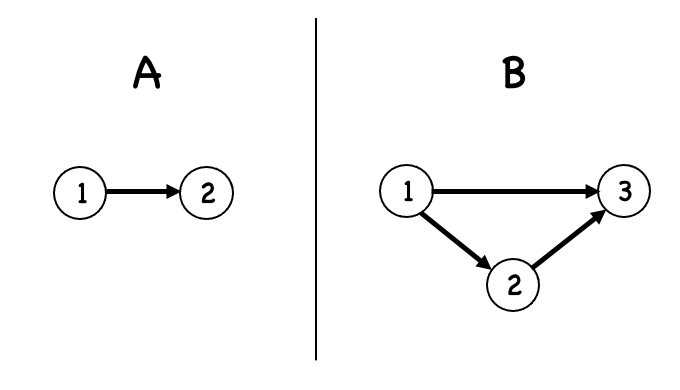
Figure 1: The graph $B$, on the right, contains a vertex with both an in-edge and an out-edge, while the graph $A$, on the left, does not.

Duplicator wins the analogous 2-round M-S game starting with these two graphs. Hence, by Theorem 1.2, the property $P$ is not expressible with just $2$ quantifiers.

1.2 Related Work in Complexity

Trees are a much studied data structure in complexity theory and logic. It is well known that it is impossible, in FOL, to express that a graph with no further relations is a tree [17, Proposition 3.20]. We note, however, that given a partial ordering on the nodes of a graph, it is easy to express in FOL the property that the partial ordering gives rise to a tree. The relevant sentence expresses that there is a root (i.e., a greatest element) from which all other nodes descend, and if a node $x$ has nodes $y$ and $z$ as distinct ancestors then one of $y$ and $z$ must have the other as its own ancestor. Hence the needed sentence is the conjunction of the following two sentences:

$$\exists x\forall y(y\neq x\rightarrow y<x),$$

$$\forall x\forall y\forall z((x<y\land x<z\land y\neq z)\rightarrow(y<z\vee z<y)).$$

There are also interesting models of computation and logics based on trees. See, for example, the literature on Finite Tree Automata [7] and Computational Tree Logic [6].

We now discuss $s$-$t$ connectivity. In this paragraph only, $n$ denotes the number of nodes in the graph and $k$ the number of edges in a shortest path from $s$ to $t$. The $s$-$t$ connectivity problem has been studied extensively in both logic [1, 15] and complexity theory. Most complexity studies of this problem have focused on space and time complexity. Directed $s$-$t$ connectivity is known to be $\mathsf{NL}$-complete (see for example Theorem 16.2 in [18]), while undirected $s$-$t$ connectivity is known to be in $\mathsf{L}$ [19]. Savitch [21] proved that $s$-$t$ connectivity can be solved in $O(\log^{2}(n))$ space and $n^{\log_{2}(n)(1+O(1))}$ time. Recent work of Kush and Rossman [16] has shown that the randomized $\mathsf{AC}^{0}$ formula complexity of $s$-$t$ connectivity is at most size $n^{0.49\log_{2}(k)+O(1)}$, a slight improvement. Barnes, Buss, Ruzzo and Schieber [2] gave an algorithm running in both sublinear space and polynomial time for $s$-$t$ connectivity. Gopalan, Lipton, and Meka [12] presented randomized algorithms for solving $s$-$t$ connectivity with non-trivial time-space tradeoffs. The $s$-$t$ connectivity problem has also been studied from the perspective of circuit and formula depth. For the weaker model of $\mathsf{AC}^{0}$ formulas an $n^{\Omega(\log(k))}$ size lower bound is known to hold unconditionally [4, 5, 20].

There is also a natural and well-known correspondence with the number of quantifiers in FOL and circuit complexity, in particular with the circuit class $\mathsf{AC}^{0}$ (constant-depth circuits comprised of NOT gates along with unbounded fan-in OR and AND gates). For example, Barrington, Immerman, and Straubing [3] proved that $\text{uniform}_{\mathsf{FO}}\text{-}\mathsf{AC}^{0}=\mathsf{FO}[<,\text{BIT}]$, thus characterizing the problems solvable in uniform $\mathsf{AC}^{0}$ by those expressible in FOL with ordering and a BIT relation.

More generally it is known that $\text{uniform}_{\mathsf{FO}}\text{-}\mathsf{AC}[t(n)]=\mathsf{FO}[<,\text{BIT}][t(n)]$ ([15], Theorem 5.22), i.e., FO formulas over ordering and BIT relations, defined via constant-sized blocks that are “iterated” for $O(t(n))$ times, are equivalent in expressibility with $\mathsf{AC}$ circuits of depth $O(t(n))$. (See Appendix C for a more detailed statement.) Generally speaking, the number of quantifiers of FOL sentences (with a regular form) roughly corresponds to the depth of a (highly uniform) $\mathsf{AC}^{0}$ circuit deciding the truth or falsity of the given sentence. Thus the number of quantifiers can be seen as a proxy for “uniform circuit depth”.

2 Difference in Magnitude: Quantifier Rank vs. Number of Quantifiers

Let $V$ be a vocabulary with at least one relation symbol with arity at least 2. It is known [8] that the number of inequivalent sentences in vocabulary $V$ with quantifier rank $k$ is not an elementary function of $k$ (that is, grows faster than any tower of exponents). Since the number of sentences in vocabulary $V$ with $k$ quantifiers is at most only double exponential in $k$ (e.g., a function that grows like $2^{2^{p(k)}}$ for some polynomial $p(k)$ – see Appendix A for a proof), it follows by a counting argument that for each positive integer $k$, there is a property $P$ of finite structures with vocabulary $V$ that can be expressed by a sentence of quantifier rank $k$, but where the number of quantifiers needed to express $P$ is not an elementary function of $k$. However, to our knowledge, up to now no explicit examples have been given of a property $P$ where the quantifier rank of a sentence to express $P$ is $k$, but where the number of quantifiers needed to express the property $P$ is at least exponential in $k$. In the proof of the following theorem, we give such an explicit example.

Let $f_{V}(k)$ be the number of structures with $k$ nodes up to isomorphism in vocabulary $V$ (such as the number of non-isomorphic graphs with $k$ nodes). Note that in the case of graphs (a single binary relation symbol), $f_{V}(k)$ is asymptotic to $(2^{k^{2}})/k!$ [13], and Stirling’s formula implies that $f_{V}(k)=2^{\Omega(k^{2})}$). We have the following theorem.

Theorem 2.1.

Assume that the vocabulary $V$ contains at least one relation symbol with arity at least 2. There is an algorithm such that given a positive integer $k$, the algorithm produces a FO sentence $\sigma$ of quantifier rank $k$ where the minimum number of quantifiers needed to express $\sigma$ in FOL is $kf_{V}(k-1)$, which grows like $2^{\Omega(k^{2})}$, and where the algorithm runs in time polynomial in the length of $\sigma$.

Proof 2.2.

For simplicity, let us assume that the vocabulary $V$ consists of a single binary relation symbol, so that we are dealing with graphs. It is straightforward to modify the proof to deal with an arbitrary vocabulary with at least one relation symbol of arity at least 2. Let us write $f$ for $f_{V}$. Let $C_{1},\ldots,C_{f(k-1)}$ be the $f(k-1)$ distinct graphs up to isomorphism with $k-1$ nodes. For each $j$ with $1\leq j\leq f(k-1)$, derive the graph $D_{j}$ that is obtained from $C_{j}$ by adding one new node with a single edge to every node in $C_{j}$. Thus, $D_{j}$ has $k$ nodes. $D_{j}$ uniquely determines $C_{j}$, since $C_{j}$ is obtained from $D_{j}$ by removing a node $a$ that has a single edge to every remaining node; even if there were two such nodes $a$, the result would be the same. Therefore, there are $f(k-1)$ distinct graphs $D_{j}$. We now give our sentence $\sigma$. Let $\sigma_{j}$ be the sentence $\exists x_{1}\cdot\cdot\cdot\exists x_{k}\tau_{j}(x_{1},\ldots,x_{k})$, which expresses that there is a graph with a subgraph isomorphic to $D_{j}$. Then the sentence $\sigma$ is the conjunction of the sentences $\sigma_{j}$ for $1\leq j\leq f(k-1)$. Since the sentence $\sigma$ is of length $2^{\Omega(k^{2})}$, it is not hard to verify that this sentence can be generated by an algorithm running in polynomial time in the length of the sentence (there is enough time to do all of the isomorphism tests by a naive algorithm).

The sentence $\sigma$ has quantifier rank $k$. As written, this sentence has $kf(k-1)$ quantifiers. Let $A$ be the disjoint union of $D_{1},\ldots,D_{f(k-1)}$. If $p$ is a point in $A$, define $B_{p}$ to be the result of deleting the point $p$ from $A$. Let $\cal{A}$ consist only of $A$, and let $\cal{B}$ consist of the graphs $B_{p}$ for each $p$ in $A$. If $p$ is in the connected component $D_{j}$ of $A$, then $B_{p}$ does not have a subgraph isomorphic to $D_{j}$. Hence, no member of ${\cal B}$ satisfies $\sigma$. Since the single member $A$ of ${\cal A}$ satisfies $\sigma$, and since no member of ${\cal B}$ satisfies $\sigma$, we can make use of M-S games played on $\cal{A}$ and $\cal{B}$ to find the number of quantifiers needed to express $\sigma$.

Assume that we have labeled copies of $A$ and the various $B_{p}$’s after $i$ rounds of an M-S game played on $\cal{A}$ and $\cal{B}$. The labelling tells us which points have been selected in each of the first $i$ rounds. Let us say that a labeled copy of $A$ and a labeled copy of $B_{p}$ are in harmony after $i$ rounds if the following holds. For each $m$ with $1\leq m\leq i$, if $a$ is the point labeled $m$ in $A$, and $b$ is the point labeled $m$ in $B_{p}$, then $a=b$. In particular, if the labeled copies of $A$ and $B_{p}$ are in harmony, then there is a partial isomorphism between the labeled copies of $A$ and $B_{p}$.

Let Duplicator have the following strategy. Assume first that in round $i$, Spoiler selects in $\cal{A}$, and selects a point $a$ from a labeled member $A$ of $\cal{A}$. Then Duplicator (by making extra copies of labeled graphs in $\cal{B}$ as needed) does the following for each labeled $B_{p}$ in $\cal{B}$. If $a\neq p$, and if the labeled copies of $A$ and $B_{p}$ before round $i$ are in harmony, then Duplicator selects $a$ in $B_{p}$, which maintains the harmony. If $a=p$, or if the labeled $A$ and $B_{p}$ before round $i$ are not in harmony, then Duplicator makes an arbitrary move in $B_{p}$.

Assume now that in round $i$, Spoiler selects in $\cal{B}$. When Spoiler selects the point $b$ from a labeled copy of $B_{p}$, then for each labeled $A$ from $\cal{A}$, if the labeled copy of $A$ is in harmony with the labeled copy of $B_{p}$ before round $i$, then Duplicator selects $b$ in $A$, and thereby maintains the harmony. We shall show shortly (Property * below) that in every round, each labeled member of $\cal{A}$ is in harmony with a labeled member of $\cal{B}$, so in the case we are now considering where Spoiler selects in $\cal{B}$, Duplicator does select a point in round $i$ in each labeled member of $\cal{A}$.

We prove the following by induction on rounds:

Property *: If $A$ is a labeled graph in $\cal{A}$ and if point $p$ in $A$ was not selected in the first $i$ rounds, then there is a labeled copy of $B_{p}$ that is in harmony with $A$ after $i$ rounds.

Property * holds after 0 rounds (with no points selected). Assume that Property * holds after $i$ rounds; we shall show that it holds after $i+1$ rounds. There are two cases, depending on whether Spoiler moves in $\cal{A}$ or in $\cal{B}$ in round $i+1$. Assume first that Spoiler moves in $\cal{A}$ in round $i+1$. Assume that point $p$ was not selected in $A$ after $i+1$ rounds. By inductive assumption, there are labeled versions of $A$ and $B_{p}$ that are in harmony after $i$ rounds. So by Duplicator’s strategy, labeled versions of of $A$ and $B_{p}$ are in harmony after $i+1$ rounds. Now assume that Spoiler moves in $\cal{B}$ in round i+1. For each labeled graph $A$ in $\cal{A}$, if a labeled $B_{p}$ is in harmony with the labeled $A$ after $i$ rounds, then by Duplicator’s strategy, the harmony continues between the labeled $A$ and $B_{p}$ after $i+1$ rounds. So Property * continues to hold after $i+1$ rounds. This completes the proof of Property *.

After $(kf(k-1))-1$ rounds, pick an arbitrary labeled graph $A$ in $\cal{A}$. Since at most $(kf(k-1))-1$ points have been selected after $(kf(k-1))-1$ rounds, and since $A$ contains $kf(k-1)$ points (because it is the disjoint union of $f(k-1)$ graphs each with $k$ points), there is some point $p$ that was not selected in $A$ in the first $(kf(k))-1$ rounds. Therefore, by Property *, a labeled version of $A$ and of $B_{p}$ are in harmony after $(kf(k))-1$ rounds, and hence there is a partial isomorphism between the labeled $A$ and $B_{p}$. So Duplicator wins the $(kf(k-1))-1$ round M-S game! Therefore, by Theorem 1.2, the number of quantifiers needed to express $\sigma$ is more than $(kf(k-1))-1$. Since $\sigma$ has $kf(k-1)$ quantifiers it follows that the minimum number of quantifiers need to express $\sigma$ is exactly $kf(k-1)$.

3 Rooted Trees

Our aim in this section is to establish the minimum number of quantifiers needed to distinguish rooted trees of depth at least $k$ from those of depth less than $k$ using first-order formulas, given a partial ordering on the vertices induced by the structure of the rooted tree. Figure 2

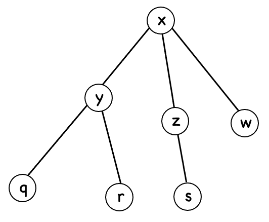
Figure 2: A rooted tree with designated root node $x$ and depth $3$.

gives an example of a tree where we designate $x$ as the root node. We define the depth of such a tree to be the maximum number of nodes in a path from the root to a leaf, where all segments in the path are directed from parent to child. Although it is more customary to denote the depth of a tree in terms of the number of edges along such a path, we keep to the above definition because we will often run into the special case of linear orders, which we view as trees in the natural way, and linear orders are characterized by their size (number of nodes) and we would like the size of a liner order to correspond to the depth of the associated tree. Let us denote the tree rooted at $x$ by $T_{x}$. We make the arbitrary choice that the node $x$ is the largest element in the induced partial order, so that for two nodes $\alpha,\beta$ of $T_{x}$, we have $\alpha>\beta$ iff there is a path $(x_{1},...,x_{n})$ in $T_{x}$ with $\alpha=x_{1}$ and $\beta=x_{n}$ such that $x_{i}$ is a parent of $x_{i+1}$ for $1\leq i\leq n-1$. Thus, for example, in Figure 2, $x>q$ and $z>s,$ etc.

The problem of distinguishing the depth of a rooted tree via a first-order formula with a minimum number of quantifiers is similar to the analogous problem for linear orders of different sizes, since a rooted tree has depth $k$ or greater iff it has a leaf node, above which there is linear order of size at least $k-1$.

Our strategy will be to characterize a tree of depth $d$ recursively as a graph containing a vertex $v$ which has a subtree of depth $k$ that includes $v$ and everything below it, and a linear order of length $d-k$ comprising the vertices above $v$, where $k$ is chosen to minimize the total number of quantifiers. We then show that this is the minimum quantifier way to characterize a tree of each given depth.

The following result is classic and key to establishing a number of fundamental inexpressibility results in FOL [17]. It is typically obtained by appeal to Theorem 1.1.

Theorem 3.1 ([17], Theorem 3.6).

Let $f(r)=2^{r}-1$. In an $r$-round E-F game played on two linear orders of different sizes, Duplicator wins if and only if the size of the smaller linear order is at least $f(r)$.

Analogs of Theorem 3.1 are proven for M-S games in [10]. The following definition and theorems are from that paper.

Definition 3.2 ([10]).

Define the function $g:\mathbb{N}\rightarrow\mathbb{N}$ such that $g(r)$ is the maximum number $k$ such that there is a formula with $r$ quantifiers that can distinguish linear orders of size $k$ or larger from linear orders of size less than $k$.

Theorem 3.3 ([10]).

The function $g$ takes on the following values: $g(1)=1,g(2)=2,g(3)=4,g(4)=10$, and for $r>4$,

$$g(r)=\begin{cases}&2g(r-1)\leavevmode\nobreak\ \leavevmode\nobreak\ \leavevmode\nobreak\ \leavevmode\nobreak\ \leavevmode\nobreak\ \leavevmode\nobreak\ \textrm{if $r$ is even,}\\ &2g(r-1)+1\textrm{ if $r$ is odd.}\end{cases}$$

Theorem 3.4 ([10]).

In an $r$-round M-S game played on two linear orders of different sizes Duplicator has a winning strategy if and only if the size of the smaller linear order is at least $g(r)$.

For given positive integers $r$ and $k$, we want to know if there exist sentences with $r$ quantifiers that distinguish rooted trees of depth $k$ or larger from rooted trees of depth smaller than $k$. For $k=r$, one such sentence is

$$\exists x_{1}\cdot\cdot\cdot\exists x_{r}\bigwedge\limits_{1\leq i<r}(x_{i}<x_{i+1}),$$ (2)

which distinguishes rooted trees of depth $r$ or larger from rooted trees of depth less than $r$. Here, if $T_{x}$ is a rooted tree of depth exactly $r$ then $x_{1}$ would be a deepest child. Since there are only finitely many inequivalent formulas in up to $r$ variables that include the relations $<$ and $=$ and at most $r$ quantifiers, there is some maximum such $k$, which we shall designate by $t(r)$. With $\mathbb{N}=\{1,2,...\}$, we restate this definition of $t$ formally as follows. Note that no meaningful sentence about trees can be constructed with a single quantifier, so the definition begins at $r=2$.

Definition 3.5.

Define the function $t:\{2,3,...\}\rightarrow\mathbb{N}$ such that $t(r)$ is the maximum number $z$ such that there is a formula with $r$ quantifiers that can distinguish rooted trees of depth $z$ or larger from rooted trees of depth less than $z$.

By (2) above, $t(r)\geq r$ for $r\geq 2$. For an M-S game of $r$ rounds on rooted trees of sizes $t(r)$ or larger on one side, and $t(r)-1$ or smaller on the other side, by the Equivalence Theorem, Spoiler will have a winning strategy.

Since linear orders are perfectly good rooted trees, we have the following:

For all $r$ we have $t(r)\leq g(r)$.

In the subsections that follow on rooted trees we sometimes refer to the deeper tree or family of trees in a given multi-structural game by $B$ (for “Big”) and the shallower tree/family of trees by $L$ (for “Little”). Analogously, when considering games on linear orders, $B$ often refers to the bigger linear order(s) and $L$ the littler one(s). Further, on linear orders of some size, a designation of the form L4, say, refers to the $4$th smallest element of $L$ and analogously B4 to the $4$th smallest element of $B$. If we have to refer to an element in a variable position, say in the $k+1$st position of $L$, we would write $L(k+1)$.

3.1 Establishing $t(2)$ and $t(3)$

We establish upper bounds of the form $t(r)\leq k$ by finding specific trees of depths $k$ and $k^{\prime}>k$, and then finding Duplicator-winning strategies for the associated $r$-round multi-structural game on these trees.

Definition 3.6.

By $T_{x}(d)$ we mean a tree rooted at $x$ of depth $d$. Analogously, $T_{x}(d+)$ means that the tree rooted at $x$ has depth $d$ or greater, and $T_{x}(<d)$ means that the tree has depth less than $d$.

Lemma 3.7.

$t(2)=2$.

Proof 3.8.

The formula $\Upsilon_{2}=\exists x\exists y(x<y)$ distinguishes $T_{x}(<2)$ from $T_{x}(2+)$ and so $t(2)\geq 2$. The upper bound $t(2)\leq g(2)=2$ follows from Observation 3 and the known value of $g(2)$ given by Theorem 3.3.

Lemma 3.9.

$t(3)=4$.

Proof 3.10.

The inequality $t(3)\leq g(3)=4$ follows from Observation 3 and the value of $g(3)$ given by Theorem 3.3. To establish $t(3)\geq 4$, let us look at the two different expressions that distinguished linear orders of size at least $4$ from those of size less than $4$:

$$\Phi_{3,\forall}=\forall x\exists y\exists z( x<y<z\vee y<z<x)$$ (3)

$$\Phi_{3,\exists}=\exists x\forall y\exists z($$ (4)

$$y<x\rightarrow z>x\leavevmode\nobreak\ \leavevmode\nobreak\ \leavevmode\nobreak\ \land$$

$$y>x\rightarrow(z\neq y\land z>x)\leavevmode\nobreak\ \leavevmode\nobreak\ \leavevmode\nobreak\ \land$$

$$y=x\rightarrow z<x)$$

Note that $\Phi_{3,\forall}$, a statement that says that for every $x$ there are either two elements less than $x$ or two elements greater than $x$, fails for the rooted tree of depth $4$ in Figure 3,

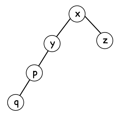
Figure 3: A rooted tree of depth $4$ that does not satisfy $\Phi_{3,\forall}$.

since the vertex $z$ fails to satisfy this condition, and hence is not a viable candidate for a formula that distinguishes $T_{x}(4+)$ from $T_{x}(<4)$. However, $\Phi_{3,\exists}$ does succeed in this regard, since it says that there is an element that has one smaller element and two larger elements. A rooted tree of depth $4$ always has such an element – the parent of a deepest leaf node – the element labeled $p$ in the figure. Further, $\Phi_{3,\exists}$ is satisfied by every rooted tree of depth at least $4$ and no rooted tree of depth less than $4$. The lemma follows.

3.2 Establishing $t(4)$

Definition 3.11.

By l.o.(k) we mean the unique linear order with $k$ nodes.

Lemma 3.12.

$t(4)\leq 8$.

Proof 3.13.

We first show that Duplicator can win a $4$-round multi-structural game on the pair of rooted trees of depths $9$ and $10$ depicted in Figure 4.

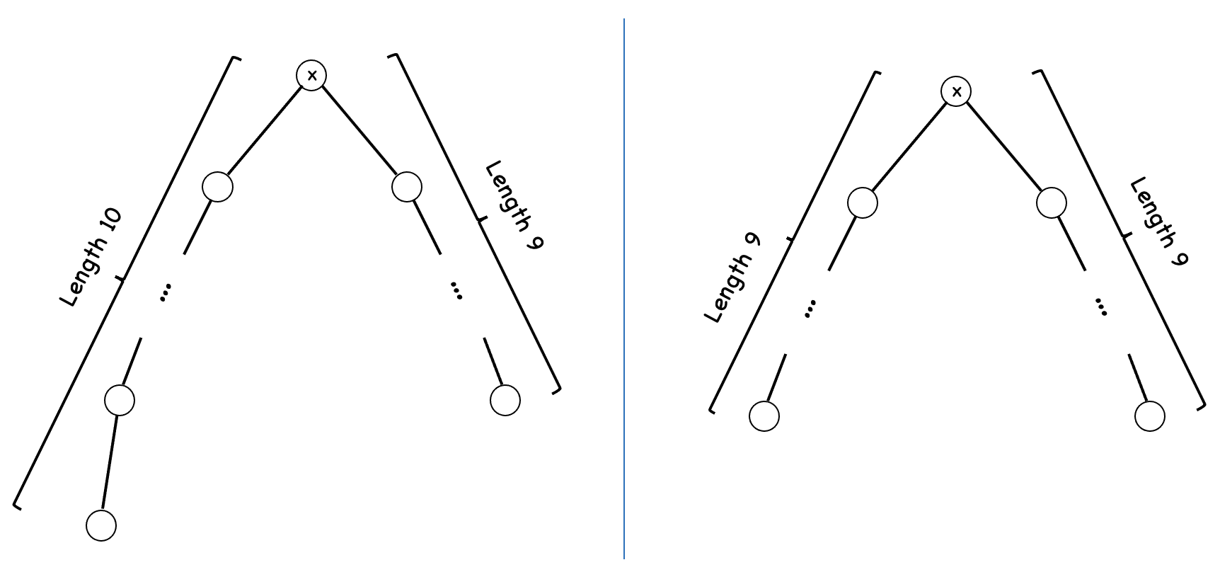
Figure 4: The case of $T_{x}(10)$ (left-hand side) vs. $T_{x}(9)$ (right-hand side). The rooted tree, $T_{x}(10)$, has two branches, one of length $10$, the other of length $9$. The rooted tree, $T_{x}(9)$, has two branches each of length $9$.

If Spoiler plays his first move on $L$, any move choice is mirrored with a symmetrical move on the length-$9$ branch of $B$ and Spoiler’s 1st move is essentially wasted. Hence, Spoiler’s best move is on the length-$10$ branch of $B$. It is then easy to see that the remainder of the game can be assumed to be played completely on the length-$10$ branch of $B$ and one of the length-$9$ branches of $L$, so that in effect we are playing a $10$ vs. $9$ linear order game where Spoiler plays first on $B$.

Let $B$ now stand for a linear order of size $10$ (i.e., the left branch of $T_{x}(10)$) and $L$ stand for a linear order of size $9$ (i.e., the left branch of $T_{x}(9)$). If Spoiler plays on $B$ leaving a short side of $3$ or less then Duplicator can match the short side play on a single copy of $L$ and reach a position with long sides of size $6+$ vs. $5+$ and so reach a position that is easily seen to be Duplicator-winning by direct play-out. Thus, WLOG, we may assume Spoiler plays B5, in which case Duplicator will respond by playing on two copies of $L$, playing L5 on one and L4 on the other, as in Figure 5,

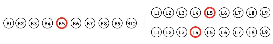
Figure 5: The $T_{x}(10)$ vs. $T_{x}(9)$ game turns into an l.o.(10) vs. l.o.(9) game where Spoiler is constrained to play first on l.o.(10). A most challenging move is to play B5, to which Duplicator responds playing L4 on one copy of $L$ and L5 on another.

in one case matching the short side of the main $B$ branch, and in the other case matching the long side of the main $B$ branch. Although Duplicator can always play with the oblivious strategy, in this case playing just these two moves suffices and simplifies our analysis. If Spoiler now makes his 2nd round play on $B$, a move to the left or on top of B5 is matched with an identical move on the first copy of $L$, while a move to the right of B5 is matched with identical long-side move on a second copy of $L$. In either case Duplicator easily survives another two rounds just on a single pair of structures. Suppose instead that on his 2nd move, Spoiler plays on $L$. He will clearly want to play on the non-matched sides of each copy of $L$, in other words, playing on L6-L9 on the top copy of $L$ and on L1-L3 on the bottom $L$ copy. (Otherwise he will just transpose into a case considered a moment ago, when Spoiler played his 2nd round move on $B$.) For this analysis Duplicator can ignore the bottom copy of $L$ since she just needs to maintain a single isomorphism. If Spoiler plays L6, Duplicator responds with B6 and clearly survives two more rounds, while a Spoiler move of L7 meets with a Duplicator response of B7, again surviving $2$ more rounds. Spoiler moves of L8 or L9 are met symmetrically with B9 or B10 respectively. Thus Duplicator survives the l.o.($10$) vs. l.o.($9$) game where Spoiler must play first on l.o.($10$) and hence Duplicator also survives the $T_{x}(10)$ vs. $T_{x}(9)$ game. Thus $t(4)\leq 9$.

It would be nice, at this point, if we could claim that $t(4)=9$ by using our expression that established $t(3)\geq 4$ to say that there is an element $w$ with a rooted tree of size at least $4$ both above and below $w$, and in this way differentiate $T_{x}(9+)$ from $T_{x}(<9)$. However, things are not that easy; the expression (4), which established $t(3)\geq 4$, started with an existential quantifier, and the logical expression we would end up using to mimic the aforementioned English language expression would start with two existential quantifiers, and so we wouldn’t be able to use it to capture the “both above and below” part of the English language expression.

With the failure of this attempted logical expression in the back of our minds, consider the case of $T_{x}(9)$ vs. $T_{x}(8)$ where we pick trees in the same basic model as the $T_{x}(10)$ vs. $T_{x}(9)$ trees, but with a bit more nuance. See Figure 6.

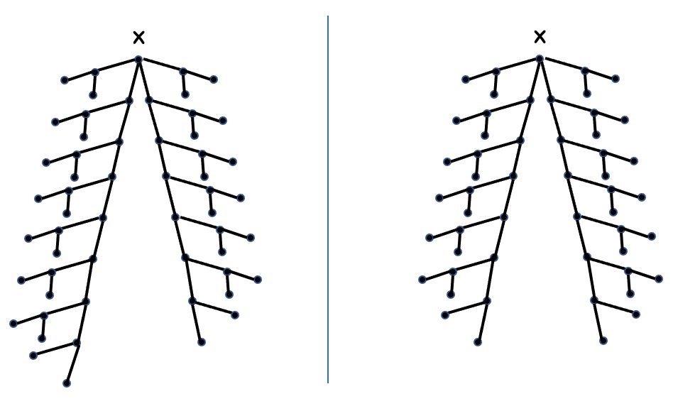
Figure 6: More nuanced rooted trees in the $T_{x}(9)$ (left-hand side) vs. $T_{x}(8)$ (right-hand side) game.

The left hand main branch of the left hand tree is of length $9$ while all other main branches of the two trees are of length $8$. As earlier, it is wasteful for Spoiler to play his 1st round move on any of the main branches of length $8$ or their offshoots, and a most challenging move is to select the mid-point along the main $9$ branch in $B$. In essence Spoiler is trying to force the play of a $9$ vs. $8$ linear order game in which he is forced to play first on $L$ – which indeed would be Spoiler-winning. However, as we shall see, the more nuanced trees in Figure 6 provide just enough additional detail so that Duplicator can foil this strategy (because there is now not just a linear order below the selected 1st round nodes, but rooted trees). In response, Duplicator will make a second copy of $L$ and play on the 4th element along one of the length $8$ branches in the first copy, call this copy $L_{1}$, and the 5th element along one of the length $8$ branches in the second copy, which we will refer to as $L_{2}$. See Figure 7.

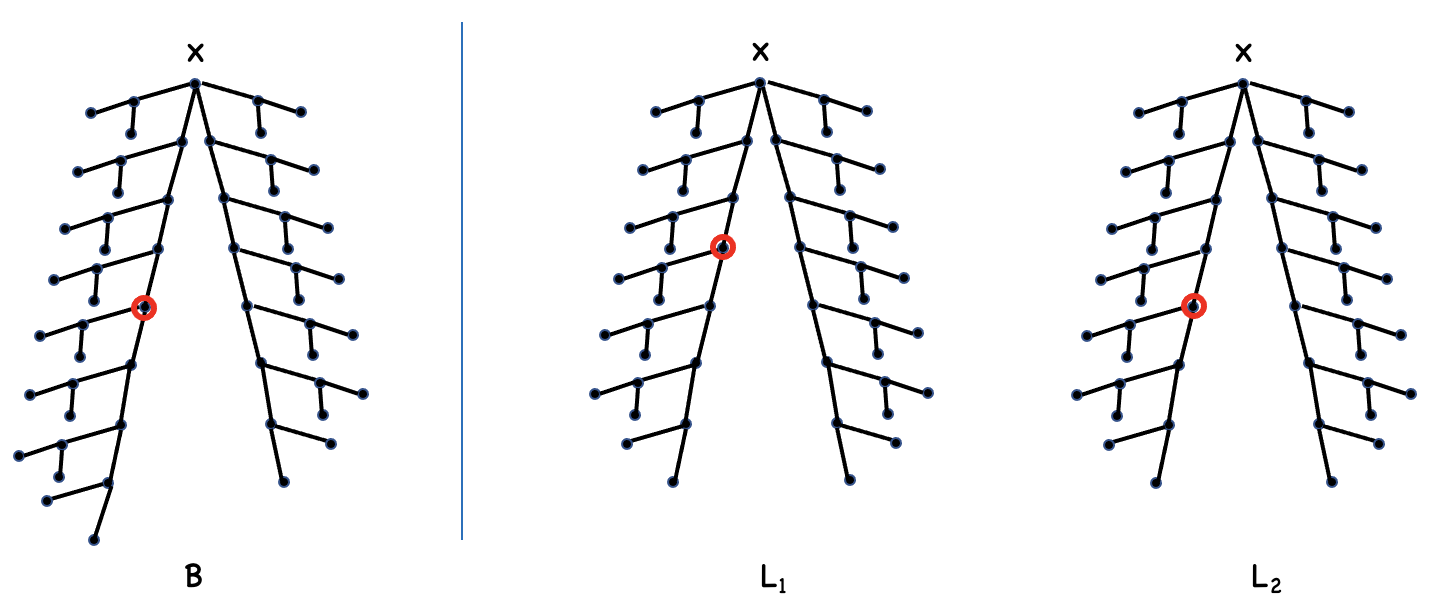
Figure 7: The $T_{x}(9)$ vs. $T_{x}(8)$ game after Spoiler plays the midpoint along the long branch of $B$, while Duplicator makes a second copy of $L$ and plays on the 4th element along one of the length $8$ branches in the first copy, which we call $L_{1}$, and the 5th element along one of the length $8$ branches in the second copy, which we call $L_{2}$.

If Spoiler is to win in the sub-game of $B$ vs. $L_{2}$ he must be able to win a $3$-round game on the sub-tree below where the first moves were played on these two trees, with the addition of the ability to play on top of a 1st round move, if necessary. Our aim will be to simply show that Spoiler cannot win in the remaining $3$ rounds in a game of just $B$ vs. $L_{2}$ by playing first on $L_{2}$. Suppose otherwise, and note that directing play to the 3-node sub-trees that are depicted to the left of the 1st round-selected nodes is not helpful to Spoiler so we may safely ignore those nodes. The critical sub-trees and Duplicator color-coded responses to the various possible Spoiler 2nd round moves on $L_{2}$ are given in Figure 8.

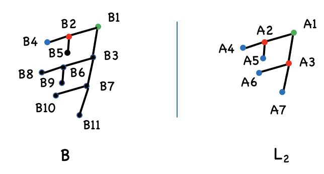
Figure 8: The critical sub-trees and Duplicator color-coded responses to the various possible Spoiler 2nd round moves on $L_{2}$

(We will consider Spoiler 2nd round moves on $B$ in just a moment.) The selection of a node from $L_{2}$ by Spoiler is responded to by Duplicator by selecting the node of the same color in $B$. It is easy to see that Duplicator wins in all cases with one minor exception, namely when Spoiler plays, say, A3, Duplicator responds with B2 and now Spoiler plays either either B6 or B7, say B6. In response to such a move, Duplicator must make a copy of $L_{2}$ and play A2 on one copy and a move such as A4 on the other copy. The move A2 safeguards against a follow-up of B8 or B9, while A4 safeguards against a follow-up of B3, B7, B10 or B11. It is thus evident that in order for Spoiler to win the $B$ vs. $L_{2}$ sub-game he must play his 2nd round move on $B$ and select and element somewhere below the element selected in the 1st round. But the only way Spoiler can win the $B$ vs. $L_{1}$ sub-game is to force the last three moves to be played in the linear orders above the 1st round moves, which now is not possible. Hence Duplicator can win the $T_{x}(9)$ vs. $T_{x}(8)$ game and so $t(4)\leq 8$ and the lemma is established.

Lemma 3.14.

$t(4)\geq 8$.

Proof 3.15.

The following sentence, with $4$ quantifiers, distinguishes rooted trees of depth $8$ or greater from those of depth less than $8$:

$$T_{4}=\exists w\forall x\exists y\exists z($$ (5)

$$x>w\rightarrow x<y<z\vee w<y<z<x$$ (6)

$$x<w\rightarrow w>y>x\vee x>y>z$$ (7)

$$x=w\rightarrow y<w\land w<z).$$ (8)

This sentence says that there exists an element $w$ with a linear order of length $4$ above it, and a rooted tree of depth $3$ below it. The condition attached to the equality condition $x=w$ is also important, and we explain that in a moment too. First, the condition (6) is the analog of equation (3), for $\Phi_{3,\forall}$, described earlier, but relativized to say that there is a linear order of length at least $4$ “above” our chosen element $w$. The condition (7) says that there is a tree of depth at least $3$ below $w$ by virtue of saying that for every element $x$ below $w$, there is either one element above $x$ and below $w$, or else that there are two additional elements below $x$, one, call it $y$, which is below $w$ and another, call it $z$, which is below $y$. With just the $x>w$ and $x<w$ implications, we are not guaranteed that there are actually any elements meeting the $x>w$ or $x<w$ conditions. The $x=w$ implication guarantees that there actually are elements meeting both of these conditions. The lemma follows.

Corollary 3.16.

$t(4)=8$.

3.3 Establishing $t(r)$ – Generic Case

In the proof of Theorem 3.3 [10], the authors provide explicit sentences that distinguish linear orders of size $g(r)$ or greater from those of size less than $g(r)$. From the proof of their Theorem 1.6, it can be seen that the distinguishing sentences $\Phi_{r}$, for $r>4$ take the form:

$$\Phi_{r}=\begin{cases}\exists x_{1}\forall x_{2}\cdot\cdot\cdot\forall x_{r-1}\exists x_{r}\phi_{r}\leavevmode\nobreak\ \leavevmode\nobreak\ \leavevmode\nobreak\ \leavevmode\nobreak\ \leavevmode\nobreak\ \textrm{for }r\textrm{ odd,}\\ \forall x_{1}\exists x_{2}\cdot\cdot\cdot\forall x_{r-1}\exists x_{r}\phi_{r}\leavevmode\nobreak\ \leavevmode\nobreak\ \leavevmode\nobreak\ \leavevmode\nobreak\ \leavevmode\nobreak\ \textrm{for }r\textrm{ even,}\end{cases}$$

where $\phi_{r}$ is quantifier-free. For odd $r$, the formula $\Phi_{r}$ says that there exists a point $x_{1}$, with a linear order of size at least $\lfloor\frac{r}{2}\rfloor$ to both sides of $x_{1}$. For even $r$, the formula $\Phi_{r}$ says that for all $x_{1}$, there exists a linear order of at least size $\frac{r}{2}$ to one side or the other of $x_{1}$.

Let us denote by $t_{\forall}(r)$ the maximum number $k$ such that rooted trees of depth $k$ and above can be distinguished from rooted trees of depth less than $k$ using prenex formulas with $r$ quantifiers beginning with a universal quantifier. Equivalently, $t_{\forall}(r)=k$ is the largest depth of a rooted tree such that Spoiler has a winning strategy on $r$-round M-S games played on rooted trees of depth $k$ or greater versus those of depth less than $k$ when his first move is constrained to be on the tree of lesser depth. Analogously, when considering linear orders, let $g_{\forall}(r)$ and $g_{\exists}(r)$ denote, respectively, the maximum number $k$ such that linear orders of size $k$ and above can be distinguished from linear orders of size less than $k$ using prenex formulas with $r$ quantifiers beginning, respectively, with a universal or existential quantifier.

Lemma 3.17.

For $r>1$, one has $t_{\forall}(r)=t(r-1)+1$.

Proof 3.18.

Given an $r$-round multi-structural game played on rooted trees of depth $k$ and $k+1$, we can choose two rooted trees, identical to the two trees in Figure 6 of Appendix 3.2, but with main branches of lengths $k+1$ and $k$ rather than $9$ and $8$. Note that a Spoiler 1st move on the smaller tree is completely wasted unless the move chosen is the top node. Choosing any other node on the smaller tree can be exactly mirrored by playing the analogous move on the right hand side of the big tree. To establish a non-isomorphism, Spoiler must force play to the left hand side of the deeper tree, after which, play on the right hand side would be of no consequence. In response to a top node 1st move, Duplicator will be forced to choose the top node from the larger tree. The problem then reduces to distinguishing a tree of depth $k-1$ (the sub-tree whose top node is just below the top node along the longest branch) vs. trees of depth $k-2$, but where Spoiler may now play anywhere. The lemma follows.

Lemma 3.19.

For $r\geq 2$, the following hold:

$$g_{\exists}(2r) =2g_{\forall}(2r-1)+1,$$ (9)

$$g_{\forall}(2r+1) =2g_{\exists}(2r).$$ (10)

Further, there are expressions establishing the $g_{\exists}$ relations having prenex signatures $\exists\forall\cdot\cdot\cdot\exists\forall\exists\exists$ with $r-1$ iterations of the $\exists\forall$ pair and then a final $\exists\exists$, while there are expressions establishing the $g_{\forall}$ relations having prenex signatures $\forall\exists\cdot\cdot\cdot\forall\exists\exists$ with $r$ iterations of the $\forall\exists$ pair and then a final $\exists$.

Proof 3.20.

We prove these relations by simultaneous induction, starting with the base case of $g_{\exists}(4)=2g_{\forall}(3)+1$. The inequality $g_{\forall}(3)\geq 4$ follows from (3), while $g_{\forall}(3)\leq g(3)=4$ so that $g_{\forall}(3)=4$, and we must therefore establish that $g_{\exists}(4)=9$. In what follows, we imagine our linear orders stretching from left (the smallest element) to right (the largest element). After an element is selected in a given round, we refer to the two remaining “sides” after playing that element as the elements that are either all smaller than (and hence to the left of) the selected element or all greater than (and hence to the right of) the selected element. We certainly can write an expression stating that “there exists an $x$ with a linear order of size $g_{\forall}(3)$ to either side” so that $g_{\exists}(4)\geq 9$. Equality is established by showing that Duplicator wins the $4$-round l.o.(10) vs. l.o.(9) game with Spoiler constrained to play first on $B$ – but this is precisely what is shown in the second paragraph of the proof of Lemma 3.12.

The general (inductive) $g_{\exists}(2r)$ argument is essentially the same argument as we have just given. Instead of arriving at an l.o.(5) vs. l.o.(4) $3$-round game we arrive at an $(r-1)$-round l.o.($g_{\forall}(2r-1)+1$) vs. l.o.($g_{\forall}(2r-1)$) game where Spoiler must play first on $L$, which is Duplicator-winnable by the induction hypothesis.

For the $g_{\forall}(2r+1)$ argument we consider linear orders of sizes $2g_{\exists}(2r)$ and $2g_{\exists}(2r)+1$ where Spoiler must play first on $L$. Spoiler’s best move is to play $L(g_{\exists}(2r))$ (or $L(g_{\exists}(2r)+1)$) since Duplicator will always respond by matching the shorter side of any play thereby forcing further play to the longer side and hence Spoiler is best off keeping the two sides as balanced as possible. Duplicator will then respond by playing $B(g_{\exists}(2r))$ on one copy of $B$ and $B(g_{\exists}(2r)+1)$ on a second copy. Spoiler then must play next on $B$ and try to win a $2r$-round l.o.($g_{\exists}(2r)+1$) vs l.o.($g_{\exists}(2r)$) game. But this game is Duplicator-winnable by the induction hypothesis.

To establish the result about the prenex signatures, observe that the argument got bootstrapped from the expression (3) for $g_{\forall}(3)$, which has prenex signature $\forall\exists\exists$. Putting together $g_{\exists}(2r)$ from the two copies of $g_{\forall}(2r-1)$ tacks an $\exists$ on the front: we have an expression $\exists x_{1}(\forall x_{2}\exists x_{3}\exists x_{4}\phi\land\forall x_{2}\exists x_{3}\exists x_{4}\phi^{\prime})$ where $\phi$ and $\phi^{\prime}$ are the analogs of (3), saying that there is a linear order above and below $x_{1}$. We pull the sequence of quantifiers $\forall x_{2}\exists x_{3}\exists x_{4}$ out in front as follows:

$$\exists x_{1}\forall x_{2}\exists x_{3}\exists x_{4}(x_{2}<x_{1} \rightarrow x_{2}<x_{3}<x_{4}<x_{1}\vee x_{3}<x_{4}<x_{2}<x_{1}\leavevmode\nobreak\ \leavevmode\nobreak\ \land$$ (11)

$$x_{2}>x_{1} \rightarrow x_{1}<x_{2}<x_{3}<x_{4}\vee x_{1}<x_{3}<x_{4}<x_{2}\leavevmode\nobreak\ \leavevmode\nobreak\ \land$$ (12)

$$x_{2}=x_{1} \rightarrow x_{3}>x_{1}\land x_{4}<x_{1}).$$ (13)

Condition (11) says that, assuming there is an element smaller than $x_{1}$, then there is a linear order of size $3$ smaller than $x_{1}$. Condition (12) says that, assuming there is an element larger than $x_{1}$, then there is a linear order of size $3$ larger than $x_{1}$. The equality condition (13) guarantees that there are elements both greater than and less than $x_{1}$. In an analogous fashion one may put together $g_{\forall}(2r+1)$ from two copies of $g_{\exists}(2r)$ by tacking on a $\forall$ in front. The lemma follows.

Theorem 3.21.

For $r\geq 2$, the following holds:

$$t(r)=g_{\forall}(r-1)+t_{\forall}(r-1)+1=g_{\forall}(r-1)+t(r-2)+2.$$ (14)

If $r$ is odd, then $g_{\forall}(r-1)=g(r-1)$ so for $r$ odd we have:

$$t(r)=g(r-1)+t_{\forall}(r-1)+1=g(r-1)+t(r-2)+2.$$ (15)

Proof 3.22.

The first-order sentence establishing the lower bound associated with (14), in other words where the left hand equality symbol is replaced by $\geq$, says that “there exists an element $x$ with a linear order of size $g_{\forall}(r-1)$ above it, and a rooted tree of depth $t_{\forall}(r-1)$ below it.” Lemma 3.19 established the prenex signature $\forall\exists\cdot\cdot\cdot\forall\exists\exists$ for the expressions $g_{\forall}(r-1)$ in case $r-1$ is odd. If $r-1$ is even, the Fagin et al. paper [10] established the prenex signature $\forall\exists\cdot\cdot\cdot\forall\exists$ for $g(r-1)$, starting with $r-1=4$. It follows that $g_{\forall}(r-1)=g(r-1)$ for such values and so the formula establishing $g_{\forall}(r-1)$ has this same prenex signature for even values of $r-1$. In case $r-1=2$, the value $g(2)$ can be established via the sentence $\forall x\exists y(x<y\vee y<x)$, so that here again $g(2)=g_{\forall}(2)$ is established via a sentence of the same prenex signature.

On the other hand, $t_{\forall}(3)\geq 3$ is established via the sentence $\forall x\exists y\exists z(x<y\vee y<z<x)$ with prenex signature $\forall\exists\exists$, while $t(3)\geq 4$ is established via the expression (4), with prenex signature $\exists\forall\exists$, and hence, by the proof of Lemma 3.17, the lower bound for $t_{\forall}(4)$ is established via the prenex signature $\forall\exists\forall\exists$. The first-order sentence, described in English at the beginning of this proof, provides a means for turning an expression for $t_{\forall}(r)$ of a given prenex signature into an expression for $t(r+1)$ with the same prenex signature but with a leading $\exists$ added. By the proof of Lemma 3.17, $t_{\forall}(r+2)$ is then obtained by tacking another $\forall$ in front. Hence the expressions for $t_{\forall}(r)$ maintain consistent prenex signatures based on their parity, and $t_{\forall}(r)$ and $g_{\forall}(r)$ will inductively have identical prenex signatures as long as we can, simultaneously, inductively establish the theorem.

We thus define the expressions $\Phi_{r-1,\forall}$ for $g_{\forall}(r-1)$, and $\Upsilon_{r-1,\forall}$ for $t_{\forall}(r-1)$, inductively with the same prenex signatures, e.g.,

$$\Phi_{r-1,\forall} = \forall x_{r-1}\exists x_{r-2}\cdot\cdot\cdot\exists x_{1}\phi_{r-1,\forall}$$ (16)

$$\Upsilon_{r-1,\forall} = \forall x_{r-1}\exists x_{r-2}\cdot\cdot\cdot\exists x_{1}\tau_{r-1,\forall},$$ (17)

where $\phi_{r-1,\forall}$ and $\tau_{r-1,\forall}$ are quantifier-free. In order to form the expression $\Upsilon_{r}$ for $t(r)$, we must relativize both $\phi_{r-1,\forall}$ and $\tau_{r-1,\forall}$ so that for the new $x_{r}$ (“$x$” in the English language sentence at the beginning of the proof), $\phi_{r-1,\forall}$ applies for values of $x_{r-1}$ that are greater than $x_{r}$, while $\tau_{r-1,\forall}$ applies for values of $x_{r-1}$ that are less than $x_{r}$. Moreover, in the relativized expression for $\phi_{r-1,\forall}$ all variables $x_{1},...,x_{r-2}$ must be constrained to be greater than $x_{r}$, while in the relativized expression for $\tau_{r-1,\forall}$ all variables $x_{1},...,x_{r-2}$ must be constrained to be less than $x_{r}$. Let us refer to these relativized versions of $\phi_{r-1,\forall}$ and $\tau_{r-1,\forall}$ as $\phi^{rel}_{r-1,\forall}$ and $\tau^{rel}_{r-1,\forall}$ respectively. With these relative expressions we are able to pull out all of the quantifiers and obtain the expression $\Upsilon_{r}$ for $t(r)$ as follows:

$$\Upsilon_{r}=\exists x_{r}\forall x_{r-1}\exists x_{r-2}\cdot\cdot\cdot\exists x_{1}( x_{r-1}>x_{r}\rightarrow\phi^{rel}_{r-1,\forall}\leavevmode\nobreak\ \leavevmode\nobreak\ \land$$

$$x_{r-1}<x_{r}\rightarrow\tau^{rel}_{r-1,\forall}).$$

This expression establishes that for $r\geq 2$, we have $t(r)\geq g_{\forall}(r-1)+t_{\forall}(r-1)+1$. In order to establish that $t(r)\leq g_{\forall}(r-1)+t_{\forall}(r-1)+1$ we show that Duplicator can win multi-structural games on rooted trees of depths $t(r)$ and $t(r+1)$ that are the analogs of the trees in Figure 6. To have a chance of winning an $r$-round game on such symmetric trees, Spoiler must force play to the longest branch of $B$, in other words, force play to the branch of $B$ of length $g_{\forall}(r-1)+t_{\forall}(r-1)+2$. The only Spoiler move on $L$ that would force such an outcome would be to select the very top node. If this were an optimal play, then we would have $t(r)\leq t_{\forall}(r-1)+1\leq g_{\forall}(r-1)+t_{\forall}(r-1)+1$. The only other way for Spoiler to force play onto the longest branch of $B$ is for him to play his 1st move directly on $B$. If Spoiler were then to leave a linear order of size at least $g_{\forall}(r-1)+1$ above the played move, then Duplicator can make a copy of $L$ and on one copy play a move that leaves the identical tree below the played move to the tree left on $B$ and a linear order of size $g_{\forall}(r-1)$ above, and on the other copy leaves a liner order of size $g_{\forall}(r-1)+1$ above and a tree of depth one less than that left on $B$. Spoiler would then be forced to play next on $L$ and would have to win a $g_{\forall}(r-1)$ vs. $g_{\forall}(r-1)+1$ $(r-1)$-round game playing first on $L$, which is impossible by the definition of $g_{\forall}(r-1)$. On the other hand, if Spoiler leaves a tree of depth at least $t_{\forall}(r-1)+1$ below, then Duplicator wins down there by the parallel argument incorporating the definition of $t_{\forall}(r-1)$. On a branch of length at least $g_{\forall}(r-1)+t_{\forall}(r-1)+2$, leaving a linear order above of length at least $g_{\forall}(r-1)+1$ or a tree of depth $t_{\forall}(r-1)+1$ below is unavoidable. The upper bound on $t(r)$ is thus established and so, for $r\geq 2$, we have $t(r)=g_{\forall}(r-1)+t_{\forall}(r-1)+1$.

The fact that $t(r)=g_{\forall}(r-1)+t_{\forall}(r-1)+1=g_{\forall}(r-1)+t_{\forall}(r-2)+2$ follows by Lemma 3.17. If $r$ is odd then $r-1$ is even and, as we have remarked earlier in this proof, then $g_{\forall}(r-1)=g(r-1)$. The theorem follows.

Theorem 3.23.

For all $r\geq 1$ we have

$$t(2r)=\frac{7\cdot 4^{r}}{18}+\frac{4r}{3}-\frac{8}{9},\leavevmode\nobreak\ \leavevmode\nobreak\ \leavevmode\nobreak\ \leavevmode\nobreak\ t(2r+1)=\frac{8\cdot 4^{r}}{9}+\frac{4r}{3}-\frac{8}{9}.$$

Proof 3.24.

As established in Lemmas 3.7, 3.9 and Corollary 3.16 of Sections 3.1 and 3.2, we have $t(2)=2,t(3)=4$ and $t(4)=8$.

Let us consider the even case in the statement of the theorem first. By Theorem 3.21 we have the for all $r\geq 3$:

$$t(2r) =g_{\forall}(2r-1)+t(2r-2)+2$$

$$=t(4)+\sum\limits_{i=2}^{r-1}(g_{\forall}(2i+1)+2)$$

It follows from Lemma 3.19 that $g_{\forall}(3)=4$ for $r\geq 2$,

$$g_{\forall}(2r+1) = 2g_{\exists}(2r)$$ (18)

$$= 2(2g_{\forall}(2r-1)+1)$$

$$= 4g_{\forall}(2r-1)+2.$$

Solving this linear recurrence yields $g_{\forall}(2r+1)=\frac{7\cdot 4^{r}}{6}-\frac{2}{3}$. Plugging this in and simplifying gives us that for all $r\geq 1$,

$$t(2r)=\frac{7\cdot 4^{r}}{18}+\frac{4r}{3}-\frac{8}{9}.$$

An analogous argument for the odd case gives us, again for all $r\geq 1$,

$$t(2r+1)=\frac{8\cdot 4^{r}}{9}+\frac{4r}{3}-\frac{8}{9}.$$

3.4 Comparison of the Growth Rates of the Functions $f,g$ and $t$

The following table compares the values of the functions $f,g$ and $t$ for $2\leq r\leq 10$. Recall that $f(r)$ is the maximum value such that an expression of quantifier rank $r$ can distinguish linear orders of size $f(r)$ or greater from linear orders of size less than $f(r)$, while $g(r)$ is the maximum value such that an expression with $r$ quantifiers can distinguish linear orders of size $g(r)$ or greater from linear orders of size less than $g(r)$.

$r$	$f(r)$	$g(r)$	$t(r)$
2	3	2	2
3	7	4	4
4	15	10	8
5	31	21	16
6	63	42	28
7	127	85	60
8	255	170	104
9	511	341	232
10	1023	682	404

4 s-t Connectivity

In this section we explore the number of quantifiers needed to express either directed or undirected $s$-$t$ connectivity (henceforth STCON) in FOL with the binary edge relation $E$, as a function of the number $n$ of edges in a shortest path between the distinguished nodes $s$ and $t$. STCON, also known as reachability between labelled nodes $s$ and $t$, refers to the property of graphs that labelled nodes $s$ and $t$ are connected. STCON$(n)$ denotes the property that $s$ and $t$ are connected by a path of length at most $n$ edges.

In Appendix B, we show how to describe STCON$(n)$ using $2\log_{2}(n)+O(1)$ quantifiers. The following theorem generalizes that construction, to improve the number of quantifiers to $3\log_{3}(n)+O(1)$. A similar argument shows that $K\log_{K}(n)+O(1)$ quantifiers can be used for any positive integer $K$, although this quantity is minimized for $K=3$.

Theorem 4.1.

STCON(n) can be expressed with $3\log_{3}(n)+O(1)$ quantifiers.

Proof 4.2.

We shall use $\Upsilon_{i}$ to denote sentences with $i$ quantifiers, and $\tau_{j}$ to denote quantifier-free expressions, where the subscript $j$ denotes the path length characterized by $\tau_{j}$.

We start with the following simple expression stating that $s$ and $t$ are connected and $d(s,t)\leq 3$, where $d(s,t)$ denotes the length of the shortest path from $s$ to $t$:

$$\Upsilon_{2}=\exists x_{1}\exists x_{2}(\tau_{3}\vee\tau_{2}\vee\tau_{1}),$$ (19)

where:

$$\tau_{3} = E(s,x_{1})\land E(x_{1},x_{2})\land E(x_{2},t),$$ (20)

$$\tau_{2} = E(s,x_{1})\land E(x_{1},t),$$ (21)

$$\tau_{1} = E(s,t).$$ (22)

We now iteratively add three quantifiers at each stage and slot two nodes between each of the previously established nodes, as in Figure 9.

Figure 9: An illustration of slotting two nodes between each of the pre-established nodes $s,x_{1},x_{2}$ and $t$ in order to express a distance $9$, $s-t$ path, using $5$ quantifiers as in expressions (23) and (24).

We express that there is a path of length at most $9$ from $s$ to $t$, using $5$ quantifiers as follows:

$$\Upsilon_{5}=\exists x_{1}\exists x_{2}\forall x_{3}\exists x_{4}\exists x_{5}(\tau_{9}\vee\tau_{8}\vee\cdot\cdot\cdot\vee\tau_{1}).$$ (23)

In this case, we just show $\tau_{9}$. The simplifications required to get from $\tau_{8}$ down to $\tau_{4}$ are analogous to those for getting from $\tau_{3}$ down to $\tau_{1}$, but where we apply (20) – (22) separately to each of (24) – (26).

$$\tau_{9}=\quad\quad ((x_{3}=s)\rightarrow E(s,x_{4})\land E(x_{4},x_{5})\land E(x_{5},x_{1}))\leavevmode\nobreak\ \leavevmode\nobreak\ \land$$ (24)

$$((x_{3}=t)\rightarrow E(x_{1},x_{4})\land E(x_{4},x_{5})\land E(x_{5},x_{2}))\leavevmode\nobreak\ \leavevmode\nobreak\ \land$$ (25)

$$((x_{3}\neq s\land x_{3}\neq t)\rightarrow E(x_{2},x_{4})\land E(x_{4},x_{5})\land E(x_{5},t)).$$ (26)

Using $8$ quantifiers, we can slot two new nodes between each node established in the prior step, as depicted in Figure 10.

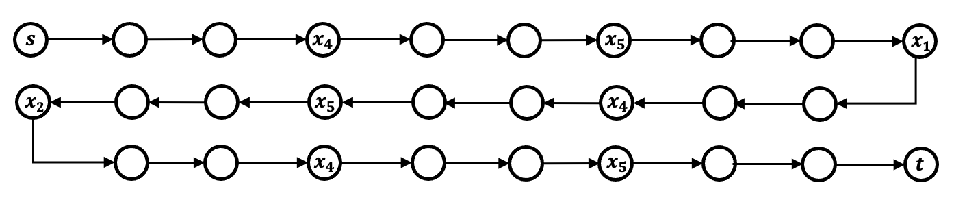
Figure 10: Slotting two nodes between each of the pre-established nodes $s,x_{1},x_{2},x_{4},x_{5}$, and $t$ in order to express a distance $27$, $s-t$ path, using $8$ quantifiers as in expressions (27) and (28)-(32).

The associated logical expression is

$$\Upsilon_{8}=\exists x_{1}\exists x_{2}\forall x_{3}\exists x_{4}\exists x_{5}\forall x_{6}\exists x_{7}\exists x_{8}(\tau_{27}\vee\tau_{26}\vee\cdot\cdot\cdot\vee\tau_{1}),\leavevmode\nobreak\ \textrm{and}$$ (27)

$$\tau_{27}=\quad\quad ((x_{3}=s\land x_{6}=s)\rightarrow E(s,x_{7})\land E(x_{7},x_{8})\land E(x_{8},x_{4}))\leavevmode\nobreak\ \leavevmode\nobreak\ \land$$ (28)

$$((x_{3}=s\land x_{6}=t)\rightarrow E(x_{4},x_{7})\land E(x_{7},x_{8})\land E(x_{8},x_{5}))\leavevmode\nobreak\ \leavevmode\nobreak\ \land$$ (29)

$$((x_{3}=s\land(x_{6}\neq s\land x_{6}\neq t))\rightarrow E(x_{5},x_{7})\land E(x_{7},x_{8})\land E(x_{8},x_{1}))\leavevmode\nobreak\ \leavevmode\nobreak\ \land$$ (30)

$$\leavevmode\nobreak\ \leavevmode\nobreak\ \leavevmode\nobreak\ \leavevmode\nobreak\ \leavevmode\nobreak\ ...$$ (31)

$$(((x_{3}\neq s\land x_{3}\neq t)\land(x_{6}\neq s\land x_{6}\neq t))\rightarrow E(x_{5},x_{7})\land E(x_{7},x_{8})\land E(x_{8},t)).$$ (32)

The expression $\tau_{27}$ will have the two “pivot points” around the universally quantified variables $x_{3}$ and $x_{6}$ and so have $3^{2}=9$ antecedent conditions corresponding to the possible ways the universally quantified variables $x_{3}$ and $x_{6}$ can each take the values $s,t$ or neither $s$ nor $t$. The right hand side of each equality condition describes how to fill in the edges in Figure 10 with two new vertices (utilizing the two newest existentially quantified variables, $x_{7}$ and $x_{8}$) and three new edges.

In this way we obtain sentences with $3n-1$ quantifiers that can express STCON instances of path length up to $3^{n}$. Thus, when $n$ is a power of $3$, we can express STCON instances of length $n$ with $3\log_{3}(n)-1\approx 1.893\log_{2}(n)-1$ quantifiers, and when $n$ is not a power of $3$, with $\lfloor 3\log_{3}(n)+2\rfloor$ quantifiers. The theorem therefore follows.

A Remark on Lower Bounds on Quantifier Rank and hence on Number of Quantifiers

Lower bounds on the number of quantifiers for $s$-$t$ connectivity follow readily from the literature. The well-known proof that connectivity is not expressible in FOL ([15, Prop. 6.15] or [17, Corollary 3.19]) can be used to establish that $s$-$t$ connectivity with path length $n$ is not expressible as a formula of quantifier rank $\log_{2}(n)-c$ for some constant $c$.

Theorem 4.3 (Immerman, Proposition 6.15 [15]).

There exists a constant $c$ such that $s$-$t$ connectivity to path length $n$ is not expressible as a formula of quantifier rank $\log_{2}(n)-c$.

Since the quantifier rank is a lower bound on the number of quantifiers, the previous theorem immediately implies a lower bound on the number of quantifiers as well. While we have shown that STCON($n$) can be expressed with $3\log_{3}(n)+O(1)$ quantifiers, we note that the minimum quantifier rank of STCON($n$) is well-known to be lower.

Theorem 4.4 ([17]).

$s$-$t$ connectivity to path length $n$ can be expressed with a formula of quantifier rank $\log_{2}(n)+O(1)$.

5 Final Comments and Future Directions

Although progress on M-S games did not come until 40 years after their initial discovery in [14], the results of this paper show that these games are quite amenable to analysis, and the more detailed information they give about the requisite quantifier structure has the potential to yield many new and interesting insights.

Theorem 2.1 tells us that the number of quantifiers can be more than exponentially larger than the quantifier rank. This shows that the number of quantifiers is a more refined measure than the quantifier rank, and gives an interesting and natural measure of the complexity of a FO formula. It would be interesting to find explicit examples where the quantifier rank is $k$, but where the required number of quantifiers grows even faster than in our example in the proof of Theorem 2.1. Ideally, we would even like to find explicit examples where the required number of quantifiers is non-elementary in $k$.

We have extended the results on the number of quantifiers needed to distinguish linear orders of different sizes [10] to distinguish rooted trees of different depths. Can this line of attack be carried further to incorporate other structures, say to other structures with induced partial orderings such as finite lattices?

The most immediate question arising from our work is whether one can improve the known upper or lower bounds on the number of quantifiers needed to express $s$-$t$ connectivity. In particular, what is the smallest constant $c\geq 1$ such that $s$-$t$ connectivity (up to path length $n$) is expressible using $c\log_{2}(n)$ quantifiers? Our Theorem 4.1 shows that $Quants(\text{STCON($n$)})$ is at most $3\log_{3}(n)+O(1)\approx 1.893\log_{2}(n)+O(1)$. The well-known lower bound of $Rank(\text{STCON($n$)})\geq\log_{2}(n)-O(1)$ (cited as Theorem 4.3) yields the only lower bound we know on $Quants(\text{STCON($n$)})$, but we also know the upper bound $Rank(\text{STCON($n$)})\leq\log_{2}(n)+O(1)$ (cited as Theorem 4.4). As these upper and lower bounds for the quantifier rank of STCON$(n)$ essentially match, in order to improve the lower bound on $Quants(\text{STCON($n$)})$ further (by a multiplicative constant), we cannot rely on a rank lower bound: we will have to resort to other methods, such as M-S games.

Another question is whether we can find other problems with even larger quantifier number lower bounds than logarithmic ones. Let us stress that substantially larger lower bounds on the number of quantifiers would have major implications for circuit complexity lower bounds. For example, by the standard way of expressing uniform circuit complexity classes in FOL [15], a property (over the $<$ relation) that requires $\log^{\alpha(n)}(n)$ quantifiers, where $\alpha(n)$ is an unbounded function of $n$, would imply a lower bound for $\text{uniform}_{\mathsf{FO}}\text{-}\mathsf{NC}$. See Appendix C for an exact statement.

Another interesting direction to push this research is to extend the notion of multi-structural games to 2nd-order logic, first-order logic with counting or to fixed point logic.

Appendix

Appendix A The Number of Sentences in Vocabulary $V$ with $k$ Quantifiers is at Most Doubly Exponential in $k$

The double exponential bound is obtained as follows. If a first-order sentence has $k$ quantifiers, then it can be written as $Q_{1}x_{1}\ldots Q_{k}x_{k}\phi$, where each $Q_{i}$ is a quantifier (either $\forall$ or $\exists$), and where $\phi$ is a quantifier-free formula in so-called full disjunctive normal form, in other words, a disjunction of conjunctions, where each possible atomic formula in $V$ appears, either negated or not negated, in each of the conjunctions. The number of possible initial quantifier sequences $Q_{1}x_{1}\ldots Q_{k}x_{k}$ is $2^{k}$. If the vocabulary $V$ has $c$ relation symbols, each of arity at most $r$, then the number $A$ of atomic formulas is at most $ck^{r}$. So the number $C$ of conjunctions, which each contain either the positive or negated form of each atomic formula, is $2^{A}$. A disjunction of these conjunctions corresponds to a selection of a subset of them and there are therefore at most $2^{C}$ of these. Hence, in total, the number of sentences with $k$ quantifiers is at most $2^{k}2^{C}=2^{k}2^{2^{A}}=2^{(k+{2^{ck^{r}}})}<2^{2^{k+ck^{r}}}$. This gives us a double exponential upper bound. Although it is not needed for our purposes, we note that a slight modification of this argument gives a double exponential lower bound, even when all of the quantifiers are existential.

Appendix B Expressing STCON(n) Using $2\log_{2}(n)+O(1)$ Quantifiers

We start by showing that we can describe STCON in the case where the number of edges, $n=2$, using a single quantifier:

$$\Phi_{1}=\exists x((E(s,x)\land E(x,t))\vee E(s,t)).$$ (33)

Here, and in subsequent expressions, the index of $\Phi_{i}$ refers to the number of quantifiers in the expression. To understand the more complicated cases it is useful to write expression (33) in the following form:

$$\Phi_{1}=\exists x(\phi_{2}\vee\phi_{1}),$$ (34)

where $\phi_{2}=E(s,x)\land E(x,t)$ is the distance-$2$ part of the unquantified expression, and $\phi_{1}=E(s,t)$ is the distance-$1$ part of the unquantified expression.

Analogously, for the case $n=4$, we have

$$\Phi_{3}=\exists x\forall y\exists z(\phi_{4}\vee\phi_{3}\vee\phi_{2}\vee\phi_{1}),$$ (35)

where $\phi_{1}$ and $\phi_{2}$ are as in (34), and

$$\phi_{4}=\quad\quad y=s\rightarrow E(s,z)\land E(z,x)\leavevmode\nobreak\ \leavevmode\nobreak\ \leavevmode\nobreak\ \land$$ (36)

$$y=t\rightarrow E(x,z)\land E(z,t),$$

$$\phi_{3}=\quad\quad y=s\rightarrow E(s,z)\land E(z,x)\leavevmode\nobreak\ \leavevmode\nobreak\ \leavevmode\nobreak\ \land$$ (37)

$$y=t\rightarrow E(x,t).$$

To understand what the above sentence is saying, consider for the moment the sentence (35), but without the disjuncts for $\phi_{3},\phi_{2}$ and $\phi_{1}$, which express that $s$ and $t$ are connected at the respective distances $3,2$ and $1$. In the sentence $\exists x\forall y\exists z\phi_{4}$, remember that we have $5$ nodes. In this sentence, we are declaring the existence of an element $x$ that is the central node in a path from $s$ to $t$, as depicted in Figure 11.

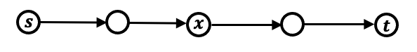
Figure 11: The five node path from $s$ to $t$, with middle node $x$.

Now $x$ is fixed, but depending on what $y$ is, $z$ can play different roles. Thus, if $y=s$ we use $z$ to guarantee a “bridge” from $s$ to $x$, in the sense of there being edges $E(s,z),E(z,x)$, and in case $y=t$, we use $z$ to guarantee a “bridge” from $x$ to $t$ in the analogous sense that there are edges $E(x,z),E(z,t)$. While the existentially quantified variable $x$ has a fixed interpretation, the universally quantified variable $y$ allows us to “pivot” in either of two directions and in so doing, the existentially quantified variable $z$ can play exactly two roles.

Returning to the expression (37), $\phi_{3}$ drops an arbitrary one of the aforementioned “bridges,” and is true if and only if $d(s,t)=3$. $\phi_{2}$ and $\phi_{1}$ were defined to support (34) and remain unchanged. Thus, in (35), $\Phi_{3}$ says that $d(s,t)$ is either $1,2,3$ or $4$ – hence that $d(s,t)\leq 4$, as claimed.

As we introduce, inductively, successive quantifier alternations, the universal quantifier will serve to provide more “pivot points” to enable exponentially more of these length-$2$ bridges, as we shall see. In turn, the existentially quantified variable following each universal quantifier will be committed to the midpoint associated with each “gap.” To see how this plays out in the case of $\Phi_{5}$, which expresses STCON when $d(s,t)\leq 8$, we have

$$\Phi_{5}=\exists x_{1}\forall x_{2}\exists x_{3}\forall x_{4}\exists x_{5}(\phi_{8}\vee\phi_{7}\vee\phi_{6}\vee\phi_{5}\vee\phi_{4}\vee\phi_{3}\vee\phi_{2}\vee\phi_{1})$$ (38)

where we have replaced the earlier variables $x,y$ and $z$ by $x_{1},x_{2}$ and $x_{3}$. In a picture, the analog of the prior Figure 11 is Figure 12.

Figure 12: The $9$ node, distance $8$, path from $s$ to $t$. The locations of $x_{1}$ and $x_{3}$ are “committed” as a result of the first three quantifiers, leaving four “gaps” that are filled as a result of the four possible “pivots” associated with the second universal quantifier – i.e., the universal quantifier quantifying over $x_{4}$.

The first universal quantifier enables a first pivot, as we saw in the expression $\exists\forall\exists\phi_{4}$, allowing two possible placements of $z$ (now labelled $x_{3}$), while the second universal quantifier enables a second pivot, which allows for four possible locations for $x_{5}$. The full expression is as follows:

$$\phi_{8}=\quad\quad (x_{2}=s\land x_{4}=s)\rightarrow E(s,x_{5})\land E(x_{5},x_{3})\leavevmode\nobreak\ \leavevmode\nobreak\ \land$$ (39)

$$(x_{2}=s\land x_{4}=t)\rightarrow E(x_{3},x_{5})\land E(x_{5},x_{1})\leavevmode\nobreak\ \leavevmode\nobreak\ \land$$ (40)

$$(x_{2}=t\land x_{4}=s)\rightarrow E(x_{1},x_{5})\land E(x_{5},x_{3})\leavevmode\nobreak\ \leavevmode\nobreak\ \land$$ (41)

$$(x_{2}=t\land x_{4}=t)\rightarrow E(x_{3},x_{5})\land E(x_{5},t).$$ (42)

Condition (39) establishes the “bridge” from $s$ to $x_{3}$, condition (40) establishes the “bridge” from $x_{3}$ to $x_{1}$, and so on. Now, for $\phi_{7}$, we replace the right hand side of (42) with $E(x_{3},t)$; for $\phi_{6}$, in addition to the replacement (42), we will replace the right hand side of (41) with $E(x_{1},x_{3})$, and analogously for $\phi_{5}$, where we will additionally replace the right hand side of (40) with $E(x_{3},x_{1})$. The expressions for $\phi_{1}$ through $\phi_{4}$ remain as previously described for $\Phi_{1}$ and $\Phi_{3}$ (but with the change of variables $x\mapsto x_{1},y\mapsto x_{2},z\mapsto x_{3}$.

Now, suppose we have defined $\Phi_{2n+1}=\exists x_{1}\forall x_{2}\cdot\cdot\cdot\forall x_{2n}\exists x_{2n+1}(\phi_{2^{n+1}}\vee\cdot\cdot\cdot\phi_{1})$. Then, as we consider $\Phi_{2n+3}$, the analog of Figure 12 is Figure 13,

Figure 13: The $2^{n+2}+1$ node, distance $2^{n+2}$, path from $s$ to $t$. The locations associated with $x_{1},x_{3},...,x_{2n+1}$ are “committed” as a result of the first $2n+1$ quantifiers, leaving $2^{n+1}$ “gaps” that are filled as a result of the $2^{n+1}$ possible “pivots” associated with the final universal quantifier – i.e., the universal quantifier quantifying over $x_{2n+2}$, which in turn determine the possible locations for $x_{2n+3}$ – the variable associated with the final existential quantifier.

and we can define

$$\Phi_{2n+3}=\exists x_{1}\forall x_{2}\cdot\cdot\cdot\forall x_{2n+2}\exists x_{2n+3}(\phi_{2^{n+2}}\vee\cdot\cdot\cdot\phi_{1}),$$ (43)

where

$$\phi_{2^{n+2}}=\quad (x_{2}=s\land x_{4}=s\land\cdot\cdot\cdot\land x_{2n+2}=s)\rightarrow E(s,x_{2n+3})\land E(x_{2n+3},x_{2n+1})\leavevmode\nobreak\ \leavevmode\nobreak\ \land$$ (44)

$$(x_{2}=s\land x_{4}=s\land\cdot\cdot\cdot\land x_{2n+2}=t)\rightarrow E(x_{2n+1},x_{2n+3})\land E(x_{2n+3},x_{2n-1})\leavevmode\nobreak\ \leavevmode\nobreak\ \land$$ (45)

$$\cdot\cdot\cdot$$

$$(x_{2}=t\land x_{4}=t\land\cdot\cdot\cdot\land x_{2n+2}=t)\rightarrow E(x_{2n+1},x_{2n+3})\land E(x_{2n+3},t).$$ (46)

Thus, for $n\geq 0$, with $2n+1$ quantifiers we can describe an STCON instance of distance $2^{n+1}$. Hence, taking logs to the base $2$, we see that we can express STCON on a graph with $n$ vertices using $2\log_{2}(n)+O(1)$ quantifiers, for a very small constant $O(1)$.

Appendix C Equivalence of First-Order Logic and Uniform Circuit Complexity Classes

Notation: By $\mathsf{FO}[\{R_{i}\}]$ we mean the set of first-order logic sentences of constant size (independent of the size of the structure) using relations $\{R_{i}\}$. By $\text{uniform}_{\mathsf{FO}}\text{-}\mathcal{C}$ we refer to the first-order uniform version of a complexity class $\mathcal{C}$. (Informally, the connection language of circuits in this class is definable by a first-order sentence. See Definition 5.17 in [15] for an exact definition.) We will always assume that our formulas have equality as a logical relation, hence whenever we have the $<$ relation we will also have the $\leq$ relation. A single binary string will be defined by a unary relation $\mathbf{1}(x)$ over the domain $[n]:=\{1,\ldots,n\}$ which is true if and only if the $x^{\textrm{th}}$ position of the binary string is a $1$. Each such relation corresponds directly to a unique $n$-bit string. In our first-order formulas over binary strings, we also allow the following relations over the domain $[n]$, with fixed interpretations:

1. $x<y$: binary relation which is true if and only if position $x$ occurs strictly before position $y$.

2. $\text{BIT}(x,y)$: binary relation which is true if and only if the $y^{\textrm{th}}$ bit of $x$ is 1.

We say that $\mathsf{FO}[<]$ is the set of first-order formulas over binary strings (represented by the relation $\mathbf{1}$) with the $<$ relation. $\mathsf{FO}[<,\text{BIT}]$ is the set of first-order formulas over binary strings (represented by $\mathbf{1}$) with both the $<$ and BIT relation.

Definition C.1 ((Definition 4.24 [15])).

Let $b:{\mathbb{N}}\rightarrow{\mathbb{N}}$. $\mathsf{FO}[\{R_{i}\}][b(n)]$ is the set of first-order logic formulas $\Phi$ (with the set of relations $\{R_{i}\}$) of the form

$$\Phi(x_{1},x_{2},\ldots,c_{k})=(\Psi_{1}(x_{1},\ldots,x_{k}))\Psi_{2}(x_{1},x_{2},\ldots,x_{k})$$

where $\Psi_{1}$, $\Psi_{2}$ are strings of logical symbols, $|\Psi_{1}|,|\Psi_{2}|,k$ are all $O(1)$ (independent of the size of the structure), and $(\Psi_{1}(x_{1},\ldots,x_{n}))\Psi_{2}(x_{1},x_{2},\ldots,x_{k})$ denotes the concatenation of $\Psi_{1}$ for $b(n)$ times followed by $\Psi_{2}$.

An important point in the above definition is that $\Psi_{1},\Psi_{2}$ are strings of logical symbols (e.g. $\exists$, $\forall$, $x$, $\vee$, $\wedge$, etc.): they need not be well-formed formulas themselves, but the concatenation $\Phi$ (as described above) must be well-formed.

To make more sense of this definition, we give a specific example. In the following example, we use . after a quantifier in the following manner: By $(\exists x.\psi_{1}(x))\psi_{2}(x)$ we mean $\exists x(\psi_{1}(x)\rightarrow\psi_{2}(x))$ and by $(\forall x.\psi_{1}(x))\psi_{2}(x)$ we mean $\forall x(\psi_{1}(x)\rightarrow\psi_{2}(x))$.

Example: We can express $s$-$t$ connectivity in a graph of size $n$ as

$$R(s,t)=(\Psi_{1}(s,t))^{\lceil\log_{2}(n)+1\rceil}\Psi_{2}(s,t)$$

where

$$\Psi_{1}(s,t)=(\exists z)(\forall a,b.((a=s\land b=z)\vee(a=z\land b=t)))(\exists s,t.(s=a\land t=b))$$

and

$$\Psi_{2}(s,t)=E(s,t)\vee(s=t).$$

Note that every formula in $\mathsf{FO}[\{R_{i}\}][b(n)]$ can be written as a formula with at most $O(b(n))$ quantifiers.

From Barrington, Immerman and Straubing [3] it is known that over the structure of binary strings, $\text{uniform}_{\mathsf{FO}}\text{-}\mathsf{AC}^{0}=\mathsf{FO}[<,\text{BIT}]$ where $\text{uniform}_{\mathsf{FO}}\text{-}\mathsf{AC}^{0}$ refers to first-order uniform $\mathsf{AC}^{0}$. In fact, for all polynomially bounded and first-order time constructible functions $t(n)$ (Theorem 5.22 [15]), $\text{uniform}_{\mathsf{FO}}\text{-}\mathsf{AC}[t(n)]$ equals $\mathsf{FO}[<,\text{BIT}][t(n)]$, where $\text{uniform}_{\mathsf{FO}}\text{-}\mathsf{AC}[t(n)]$ refers to first-order uniform $\mathsf{AC}^{0}$ circuits of depth $O(t(n))$.

Lemma C.2 (Theorem 5.22 [15]).

$\text{uniform}_{\mathsf{FO}}\text{-}\mathsf{AC}[t(n)]=\mathsf{FO}[<,\text{BIT}][t(n)]$.

Note that the above equivalence has the BIT operator, which we did not use in the rest of the paper. The rest of the section shows how to express $\text{uniform}_{\mathsf{FO}}\text{-}\mathsf{NC}$ functions (uniform circuits with $\text{polylog}(n)$ depth) without the BIT relation.

Theorem C.3.

Every circuit in $\text{uniform}_{\mathsf{FO}}\text{-}\mathsf{NC}$ over binary strings has an equivalent formula with $\text{polylog}(n)$ quantifiers using only the $<$ and $\mathbf{1}$ relations.

Proof C.4.

By Lemma C.2, every circuit in $\text{uniform}_{\mathsf{FO}}\text{-}\mathsf{NC}$ has an equivalent $\mathsf{FO}[<,\text{BIT}][\text{polylog}(n)]$ formula. By Definition C.1, every formula $\Phi(x_{1},x_{2},\ldots,x_{k})\in\mathsf{FO}[<,\text{BIT}][\text{polylog}(n)]$ can be expressed as

$$(\Psi_{1}(x_{1},x_{2},\ldots,x_{k}))^{\text{polylog}(n)}\Psi_{2}(x_{1},x_{2},\ldots,x_{k})$$

where $\Psi_{1}$, $\Psi_{2}$ are strings, and $|\Psi_{1}|,|\Psi_{2}|,k$ are all bounded by constants. Thus the BIT relation occurs at most $\text{polylog}(n)$ times in the entire formula $\Phi$. It is well-known that $\text{BIT}\in\mathsf{FO}[<][\log n]$ (Exercise 4.18 in [15]): that is, BIT can be expressed with a first-order formula of $O(\log n)$ size. Replacing each occurrence of BIT with the equivalent formula from $\mathsf{FO}[<][\log n]$ yields a formula with at most $O(\text{polylog}(n)\cdot\log(n)=\text{polylog}(n))$ quantifiers. Hence every circuit in $\text{uniform}_{\mathsf{FO}}\text{-}\mathsf{NC}$ has an equivalent formula with $\text{polylog}(n)$ quantifiers over only the $<$ relation.

References

- [1] Miklós Ajtai and Ronald Fagin. Reachability is harder for directed than for undirected finite graphs. J. Symbolic Logic, 55(1):113–150, 03 1990. URL: https://projecteuclhttps://www.overleaf.com/project/60009b2b97fcc17482762e00id.org:443/euclid.jsl/1183743189.
- [2] Greg Barnes, Jonathan F. Buss, Walter L. Ruzzo, and Baruch Schieber. A sublinear space, polynomial time algorithm for directed s-t connectivity. SIAM J. Comput., 27(5):1273–1282, 1998. URL: https://doi.org/10.1137/S0097539793283151.
- [3] David A. Mix Barrington, Neil Immerman, and Howard Straubing. On uniformity within NC. In Proceedings: Third Annual Structure in Complexity Theory Conference, Georgetown University, Washington, D. C., USA, June 14-17, 1988, pages 47–59. IEEE Computer Society, 1988. URL: https://doi.org/10.1109/SCT.1988.5262.
- [4] Paul Beame, Russell Impagliazzo, and Toniann Pitassi. Improved depth lower bounds for small distance connectivity. Comput. Complex., 7(4):325–345, 1998. URL: https://doi.org/10.1007/s000370050014.
- [5] Xi Chen, Igor Carboni Oliveira, Rocco A. Servedio, and Li-Yang Tan. Near-optimal small-depth lower bounds for small distance connectivity. In Proceedings of the 48th Annual ACM SIGACT Symposium on Theory of Computing, STOC 2016, Cambridge, MA, USA, June 18-21, 2016, pages 612–625. ACM, 2016. URL: https://doi.org/10.1145/2897518.2897534.
- [6] Edmund M. Clarke and E. Allen Emerson. Design and synthesis of synchronization skeletons using branching time temporal logic. In Workshop on the Logic of Programs, Lecture Notes in Computer Science, volume 131, pages 52–71, 1981.
- [7] Hubert Comon, Max Dauchet, Rémi Gilleroz, Florent Jacquemard, Denis Luguiez, Sophie Tison, and Marc Tommasi. Tree automata techniques and applications. http://www.eecs.harvard.edu/ shieber/Projects/Transducers/Papers/comon-tata.pdf, 1999.
- [8] A. Dawar, M. Grohe, S. Kreutzer, and N. Schweikardt. Model theory makes formulas large. In L. Arge, C. Cachin, T. Jurdziński, and A. Tarlecki, editors, ICALP07, volume 4596, pages 913–924. Springer, 2007.
- [9] Andrzej Ehrenfeucht. An application of games to the completeness problem for formalized theories. Fundamenta Mathematicae, 49:129–141, 1961.
- [10] Ronald Fagin, Jonathan Lenchner, Kenneth W. Regan, and Nikhil Vyas. Multi-structural games and number of quantifiers. In 2021 36th Annual ACM/IEEE Symposium on Logic in Computer Science (LICS), pages 1–13, 2021.
- [11] Roland Fraïssé. Sur quelques classifications des systèmes de relations. Université d’Alger, Publications Scientifiques, Série A, 1:35–182, 1954.
- [12] Parikshit Gopalan, Richard J. Lipton, and Aranyak Mehta. Randomized time-space tradeoffs for directed graph connectivity. In FST TCS 2003: Foundations of Software Technology and Theoretical Computer Science, 23rd Conference, Mumbai, India, December 15-17, 2003, Proceedings, volume 2914 of Lecture Notes in Computer Science, pages 208–216. Springer, 2003. URL: https://doi.org/10.1007/978-3-540-24597-1_18.
- [13] Frank Harary. Note on Carnap’s relational asymptotic relative frequencies. J. Symb. Log., 23(3):257–260, 1958.
- [14] Neil Immerman. Number of quantifiers is better than number of tape cells. J. Comput. Syst. Sci., 22(3):384–406, 1981.
- [15] Neil Immerman. Descriptive complexity. Graduate Texts in Computer Science. Springer, 1999. URL: https://doi.org/10.1007/978-1-4612-0539-5.
- [16] Deepanshu Kush and Benjamin Rossman. Tree-depth and the formula complexity of subgraph isomorphism. In 61st IEEE Annual Symposium on Foundations of Computer Science, FOCS 2020, Durham, NC, USA, November 16-19, 2020, pages 31–42. IEEE, 2020. URL: https://doi.org/10.1109/FOCS46700.2020.00012.
- [17] Leonid Libkin. Elements of Finite Model Theory. Texts in Theoretical Computer Science. Springer, 2012. URL: https://www.springer.com/gp/book/9783540212027.
- [18] Christos Papdimitriou. Computational Complexity. Addison-Wesley Publishing Company, Reading, MA USA, 1995.
- [19] Omer Reingold. Undirected st-connectivity in log-space. Proceedings of the 37th annual ACM symposium on the theory of computing, pages 376–385, 2005.
- [20] Benjamin Rossman. Formulas vs. circuits for small distance connectivity. In Symposium on Theory of Computing, STOC 2014, New York, NY, USA, May 31 - June 03, 2014, pages 203–212. ACM, 2014. URL: https://doi.org/10.1145/2591796.2591828.
- [21] Walter J. Savitch. Relationships between nondeterministic and deterministic tape complexities. J. Comput. Syst. Sci., 4(2):177–192, 1970. URL: https://doi.org/10.1016/S0022-0000(70)80006-X.