A multimodal tourist trip planner integrating road and pedestrian networks

Abstract

The Tourist Trip Design Problem aims to prescribe a sightseeing plan that maximizes tourist satisfaction while taking into account a multitude of parameters and constraints, such as the distances among points of interest, the expected duration of each visit, the opening hours of each attraction, the time available daily. In this article we deal with a variant of the problem in which the mobility environment consists of a pedestrian network and a road network. So, one plan includes a car tour with a number of stops from which pedestrian subtours to attractions (each with its own time windows) depart. We study the problem and develop a method to evaluate the feasibility of solutions in constant time, to speed up the search. This result is used to devise an ad-hoc iterated local search. Experimental results show that our approach can handle realistic instances with up to 3643 points of interest (over a seven day planning horizon) in few seconds.

1 Introduction

The tourism industry is one of the fast-growing sectors in the world. On the wave of digital transformation, this sector is experiencing a shift from mass tourism to personalized travel. Designing a tailored tourist trip is a rather complex and time-consuming process. Therefore, the use of expert and intelligent systems can be beneficial. Such systems typically appear in the form of ICT integrated solutions that perform (usually on a hand-held device) three main services: recommendation of attractions (Points of Interest, PoIs), route generation and itinerary customization [1]. In this research work, we focus on route generation, known in literature as the Tourist Trip Design Problem (TTDP). The objective of the TTDP is to select PoIs that maximize tourist satisfaction, while taking into account a set of parameters (e.g., alternative transport modes, distances among PoIs) and constraints (e.g., the duration of each visit, the opening hours of each PoI and the time available daily for sightseeing). In last few years there has been a flourishing of scholarly work on the TTDP [2]. Different variants of TTDP have been studied in the literature, the main classification being made w.r.t. the mobility environment which can be unimodal or multimodal [3].

In this article, we focus on a variant of the TTDP in which a tourist can move from one PoI to the next one as a pedestrian or as a driver of a vehicle (like a car or a motorbike). Under this hypothesis, one plan includes a car tour with a number of stops from which pedestrian subtours to attractions (each with its own time windows) depart. We refer to this multimodal setting as a walk-and-drive mobility environment. Our research work was motivated by a project aiming to stimulate tourism in the Apulia region (Italy). Unfortunately, the public transportation system is not well developed in this rural area and most attractions can be conveniently reached only by car or scooter, as reported in a recent newspaper article [4]: (in Apulia) sure, there are trains and local buses, but using them exclusively to cross this varied region is going to take more time than most travellers have. Our research was also motivated by the need to maintain social distancing in the post-pandemic era [5].

The walk-and-drive variant of the TTDP addressed in this article presents several peculiar algorithmic issues that we now describe. The TTDP is a variant of the Team Orienteering Problem with Time Windows (TOPTW), which is known to be NP-hard [6]. We now review the state-of-the-art of modelling approaches, solution methods and planning applications for tourism planning. A systematic review of all the relevant literature has been recently published in [2]. The TTDP is a variant of the Vehicle Routing Problem (VRP) with Profits [7], a generalization of the classical VRP where the constraint to visit all customers is relaxed. A known profit is associated with each demand node. Given a fixed-size fleet of vehicles, VRP with profits aims to maximize the profit while minimizing the traveling cost. The basic version with only one route is usually presented as Traveling Salesman Problem (TSP) with Profits [8]. Following the classification introduced in [8] for the single-vehicle case, we distinguish three main classes. The first class of problems is composed by the Profitable Tour Problems (PTPs) [9] where the objective is to maximize the difference between the total collected profit and the traveling cost. The capacitated version of PTP is studied in [10]. The second class is formed by Price-Collecting Traveling Salesman Problems (PCTSPs) [11] where the objective is to minimize the total cost subject to a constraint on the collected profit. The Price-Collecting VRPs has been introduced in [12]. Finally, the last class is formed by the Orienteering Problems (OPs) [13] (also called Selective TSPs [14] or Maximum Collection Problems [15]) where the objective is to maximize collected profit subject to a limit on the total travel cost. The Team Orienteering Problem (TOP) proposed by [16] is a special case of VRP with profits; it corresponds to a multi-vehicle extension of OP where a time constraint is imposed on each tour.
For the TTDP, the most widely modelling approach is the TOP. Several variants of TOP have been investigated with the aim of obtaining realistic tourist planning. Typically PoIs have to be visited during opening hours, therefore the best known variant is the Team Orienteering Problem with Time-Windows (TOPTW) ([17] [18], [19], [20]). In many practical cases, PoIs might have multiple time windows. For example, the tourist attraction is open between 9 am and 14 am and between 3 pm and 7 pm. In [21], the authors devise a polynomial-time algorithm for checking feasibility of multiple time windows. The size of the problem is reduced in a preprocessing phase if the PoI-based graph satisfies the triangle inequality. The model closest to the one proposed in this work is the Multi-Modal TOP with Multiple Time Windows (MM-TOPMTW) [2]. Few contributions deal with TTDP in a multimodal mobility environment. Different physical networks and modes of transports are incorporated according to two different models. The former implicitly incorporates multi-modality by considering the public transport. Due to the waiting times at boarding stops, the model is refereed to as Time-Dependent TOPTW ([22], [23], [24]). Other models incorporate the choice of transport modes more explicitly, based on availability, preferences and time constraints . In particular in the considered transport modes the tourist either walks or takes a vehicle as passenger, i.e. bus, train, subway, taxi [25],[3], [26]. To the best of our knowledge this is the first contribution introducing the TTDP in a walk-and-drive mobility environment. Other variants have been proposed to address realistic instances. Among the others, they include: time dependent profits ([27], [28], [29], [30]), score in arcs ([31]), tourist experiences ([32],[25],[3],[33]), hotel selection ([34],[35]), clustered POIs ([36],[37]).
In terms of solution methods, meta-heuristic approaches are most commonly used to solve the TTDP and its variant. As claimed in [2], Iterated Local Search (ILS) or some variations of it ([17], [24],[38], [39]) is the most widely applied technique. Indeed, the ILS provides fast and good quality solutions and, therefore, has been embedded in several real-time applications. Other solution methods are: GRASP ([33],[37]), large neighboorhod search ([40]), evolution strategy approach ([41]), tabu search ([42]), simulated annealing ([43], [44]), particle swarm optimization ([45]), ant colony optimisation([46]).
We finally observe that algorithms solving the TTDP represent one of the main back-end components of expert and intelligent systems designed for supporting tourist decision-making. Among the others they include electronic tourist guides and advanced digital applications such as CT-Planner, eCOMPASS, Scenic Athens, e-Tourism, City Trip Planner, EnoSigTur, TourRec, TripAdvisor, DieToRec, Heracles, TripBuilder, TripSay. A more detailed review of these types of tools can be found in [47], [48] and [49].

In this paper, we seek to go one step further with respect to the literature by devising insertion and removal operators tailored for a walk-and-drive mobility environment. Then we integrate the proposed operators in an iterated local search. A computational campaign on realistic instances show that the proposed approach can handle realistic instances with up to 3643 points of interests in few seconds. The paper is organized as follows. In section 2 we provide problem definition. In section 3 we describe the structure of the algorithm used to solve the TTDP. Section 4 and 5 introduce insertion and removal operators to tackle the TTDP in a walk-and-drive mobility environment. Section 6 illustrates how we enhance the proposed approach in order to handle instances with thousands of PoIs. In Section 7, we show the experimental results. Conclusions and further work are discussed in Section 8.

2 Problem definition

Let $G=(V,A)$ denote a directed complete multigraph, where each vertex $i\in V$ represents a PoI. Arcs in $A$ are a PoI-based representation of two physical networks: pedestrian network and road network. Moreover, let $m$ be the length (in days) of the planning horizon. We denote with $(i,j,mode)\in A$ the connection from PoI $i$ to PoI $j$ with transport $mode\in\{Walk,Drive\}$. Arcs $(i,j,Walk)$ and $(i,j,Drive)$ represent the quickest paths from PoI $i$ to PoI $j$ on the pedestrian network and the road network, respectively. As far as the travel time durations are concerned, we denote with $t^{w}_{ij}$ and $t^{d}_{ij}$ the durations of the quickest paths from PoI $i$ to PoI $j$ with transport mode equal to $Walk$ and $Drive$, respectively. A score $P_{i}$ is assigned to each PoI $i\in V$. Such a score is determined by taking into account both the popularity of the attraction as well as preferences of the tourist. Each PoI $i$ is characterized by a time windows $[O_{i},C_{i}]$ and a visit duration $T_{i}$. We denote with $a_{i}$ the arrival time of the tourist at PoI $i$, with $i\in V$. If the tourist arrives before the opening hour $O_{i}$, then he/she can wait. Hence, the PoI visit starts at time $z_{i}=max(O_{i},a_{i})$. The arrival time is feasible if the visit of PoI $i$ can be started before the closing hour $C_{i}$, i.e. $z_{i}\leq C_{i}$. Multiple time windows have been modelled as proposed in [50]. Therefore each PoI with more than one time window is replaced by a set of dummy PoI (with the same location and with the same profit) and with one time window each. A “max-n type” constraint is added for each set of PoIs to guarantee that at most one PoI per set is visited.

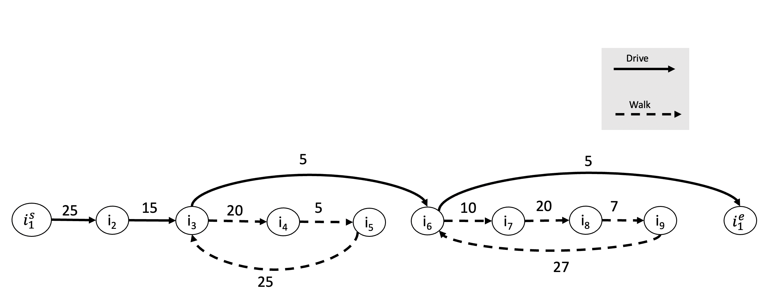
Figure 1: Example of a daily itinerary (weights on the arcs indicate travel times).

In a walk-and-drive mobility environment a TTDP solution consists in the selection of $m$ itineraries, starting and ending to a given initial tourist position. Each itinerary corresponds to a sequence of PoI visits and the transport mode selected for each pair of consecutive PoIs. As an example, Figure 1 depicts the itinerary followed by a tourist on a given day. The tourist drives from node $i^{s}_{1}$ to node $i_{3}$, parks, then follows pedestrian tour $i_{3}-i_{4}-i_{5}$ in order to visit the attractions in nodes $i_{3}$, $i_{4}$ and $i_{5}$. Hence he/she picks up the vehicle parked nearby PoI $i_{3}$ and drives to vertex $i_{6}$, parks, then follows pedestrian tour $i_{6}-i_{7}-i_{8}-i_{9}$ in order to visit the corresponding attractions. Finally the tourist picks up the vehicle parked nearby PoI $i_{6}$ and drives to the final destination $i^{e}_{1}$ (which may coincide with $i^{s}_{1}$).

Two parameters model tourist preferences in transport mode selection: $MinDrivingTime$ and $MaxWalkingTime$. Given a pair of PoIs $(i,j)$, we denote with $mode_{ij}$ the transport mode preferred by the tourist. In the following, we assume that a tourist selects the transportation mode $mode_{ij}$ with the following policy (see Algorithm 1). If $t^{w}_{ij}$ is strictly greater than $MaxWalkingTime$, the transport mode preferred by the tourist is $Drive$. Otherwise if $t^{d}_{ij}$ is not strictly greater than $MinDrivingTime$ (and $t^{w}_{ij}\leq MaxWalkingTime$), the preferred transport mode is $Walk$. In all remaining cases, the tourist prefers the quickest transport mode. It is worth noting that our approach is not dependent on the mode selection mechanism used by the tourist (i.e., Algorithm 1). A solution is feasible if the selected PoIs are visited within their time windows and each itinerary duration is not greater than $C_{max}$. The TTDP aims to determine the feasible tour that maximizes the total score of the visited PoIs. Tourist preferences on transport mode selection have been modelled as soft constraints. Therefore, ties on total score are broken by selecting the solution with the minimum number of connections violating tourist preferences.

Input: PoI $i$, PoI $j$

Output: $mode_{ij}$

1 if $t^{w}_{ij}>MaxWalkingTime$ then

2      $mode_{ij}\leftarrow Drive$;

3      

4else if $t^{d}_{ij}\leq MinDrivingTime$ then

5      $mode_{ij}\leftarrow Walk$;

6      

7else

8      

9      if $t^{w}_{ij}\leq t^{d}_{ij}$ then $mode_{ij}\leftarrow Walk$ else $mode_{ij}\leftarrow Drive$;

10      

11 end if

Algorithm 1 SelectTransportMode

2.1 Modelling transfer

Transfer connections occur when the tourist switches from the road network to the pedestrian network or vice versa. Since we assume that tourists always enter a PoI as a pedestrian, travel time $t^{d}_{ij}$ has to be increased with transfer times associated to the origin PoI $i$ and the destination PoI $j$. The former models the time required to pick up the vehicle parked nearby PoI $i$ (PickUpTime). The latter models the time required to park and then reach on foot PoI $j$ (ParkingTime). During a preprocessing phase we have increased travel time $t^{d}_{ij}$ by the (initial) PickUpTime and the (final) ParkingTime. It is worth noting that a transfer connection also occurs when PoI $i$ is the last PoI visited by a walking subtour. In this case, the travel time from PoI $i$ to PoI $j$ corresponds to the duration of a walk-and-drive path on the multigraph G: the tourist starts from PoI $i$, reaches on foot the first PoI visited by the walking subtour, then reaches PoI $j$ by driving. In Figure 1 an example of walk-and-drive path is $i_{5}-i_{3}-i_{6}$. We observe that the reference application context consists of thousands of daily visitable PoIs. Therefore, it is not an affordable option pre-computing the durations of $(|V|-2)$ walk-and-drive paths associated to each pair of PoIs $(i,j)$. For example in our computation campaign the considered $3643$ PoIs would require more than $180$ GB of memory to store about $5\cdot 10^{10}$ travel times. For these reasons we have chosen to reduce significantly the size of the instances by including in the PoI-based graph $G$ only the PickUpTime and ParkingTime. As illustrated in the following sections, walk-and-drive travel scenarios are handled as a special case of $Drive$ transport mode with travel time computed at run time.

3 Problem-solving method

Our solution approach is based on the Iterated Local Search (ILS) proposed in [17] for the TOPTW. To account for a walk-and-drive mobility environment, we developed a number of extensions and adaptations are discussed in corresponding sections. In our problem, the main decisions amount to determine the sequence of PoIs to be visited and the transport mode for each movement between pairs of consecutive PoIs. The combination of walking subtours and transport mode preferences is the new challenging part of a TTDP defined on a walk-and-drive mobility environment. To handle these new features, our ILS contains new contributions compared to the literature. Algorithm 2 reports a general description of ILS. The algorithm is initialized with an empty solution. Then, an improvement phase is carried out by combining a local search and a perturbation step, both described in the following subsections. The algorithm stops when one of the following thresholds is reached: the maximum number of iterations without improvements or a time limit. The following subsections are devoted to illustrating local search and the perturbation phase.

3.1 Local Search

Given an initial feasible solution (incumbent), the idea of local search is to explore a neighbourhood of solutions close to the incumbent one. Once the best neighboor is found, if it is better than the incumbent, then the incumbent is updated and the search restarts. In our case the local search procedure is an insertion heuristic, where the initial incumbent is the empty solution and neighbours are all solutions obtained from the incumbent by adding a single PoI. The neighbourhood is explored in a systematic way by considering all possible insertions in the current solution. As illustrated in Section 4, the feasibility of neighbour solutions is checked in constant time. As far as the objective function is concerned, we evaluate each insertion as follows. For each itinerary of the incumbent we consider a (unrouted) PoI $j$, if it can be visited without violating both its time window and the corresponding max-n type constraint. Then it is determined the itinerary and the corresponding position with the smallest time consumption. We compute the ratio between the score of the PoI and the extra time necessary to reach and visit the new PoI $j$. The ratio aims to model a trade-off between time consumption and score. As discussed in [17], due to time windows the score is considered more relevant than the time consumption during the insertion evaluation. Therefore, the POI $j^{*}$ with the highest $(score)^{2}/(extra$ $time)$ ratio is chosen for insertion. Ties are broken by selecting the insertion with the minimum number of violated soft constraints. After the PoI to be inserted has been selected and it has been determined where to insert it, the affected itinerary needs to be updated as illustrated in Section 5. This basic iteration of insertion is repeated until it is not possible to insert further PoIs due to the constraint imposed by the maximum duration of the itineraries and by PoI time windows. At this point, we have reached a local optimal solution and we proceed to diversify the search with a Solution Perturbation phase. In Section 6, we illustrate how we leverage clustering algorithms to identify and explore high density neighbourhood consisting of candidate PoIs with a ‘good’ ratio value.

3.2 Solution Perturbation

The perturbation phase has the objective of diversifying the local search, avoiding that the algorithm remains trapped in a local optima of solution landscape. The perturbation procedure aims to remove a set of PoIs occupying consecutive positions in the same itinerary. It is worth noting that the perturbation strategy is adaptive. As discussed in Section 4, in a multimodal environment a removal might not satisfies the triangle inequality, generating a violation of time windows for PoIs visited later. Since time windows are modelled as hard constraints, the perturbation procedure adapts (in constant time) the starting and ending removal positions so that no time windows are violated. To this aim we relax a soft constraint, i.e. tourist preferences about transport mode connecting remaining PoIs. The perturbation procedure finalizes (Algorithm 2 - line 2) the new solution by decreasing the arrival times to a value as close as possible to the start time of the itinerary, in order to avoid unnecessary waiting times. Finally, we observe that the parameter concerning the length of the perturbation ($\rho_{d}$ in Algorithm 2) is a measure of the degree of search diversification. For this reason $\rho_{d}$ is incremented by 1 for each iteration in which there has not been an improvement of the objective function. If $\rho_{d}$ is equal to the length of the longest route, to prevent search from restarting from the empty solution, the $\rho_{d}$ parameter is set equal to 50 $\%$ of the length of the smallest route in terms of number of PoIs. Conversely, if the solution found by the local search is the new best solution $s_{*}$, then search intensification degree is increased and a small perturbation is applied to the current solution $s^{\prime}_{*}$, i.e. $\rho_{d}$ perturbation is set to 1.

Data: MaxIter, TimeLimit

1 $\sigma_{d}\leftarrow 1$, $\rho_{d}\leftarrow 1$, $s^{\prime}_{*}\leftarrow\emptyset$, $NumberOfTimesNoImprovement\leftarrow 0$;

2 while NumberOfTimesNoImprovement $\leq$ MaxIter Or ElapTime$\leq$ TimeLimit do

3       $s^{\prime}_{*}\leftarrow InsertionProcedure(s^{\prime}_{*})$;

4       if  $s^{\prime}_{*}$ better than $s_{*}$ then

5             $s_{*}\leftarrow s^{\prime}_{*}$;

6             $\rho_{d}\leftarrow 1$;

7             $NumberOfTimesNoImprovement\leftarrow 0$;

8            

9       $NumberOfTimesNoImprovement\leftarrow NumberOfTimesNoImprovement+1$;

10       $\rho_{d}\leftarrow\rho_{d}+1$;

11       if $\rho_{d}\geq$ Size of biggest itinerary then

12             $\rho_{d}\leftarrow\max(1,\lfloor$ (Size of smallest itinerary)$/2\rfloor)$;

13            

14       end if

15      $\sigma_{d}\leftarrow\sigma_{d}+\rho_{d}$;

16       $\sigma_{d}\leftarrow\sigma_{d}$ $mod$ (Size of smallest itinerary);

17       $s^{\prime}_{*}\leftarrow$PerturbationProcedure($s^{\prime}_{*}$,$\rho_{d}$,$\sigma_{d}$);

18       Update ElapTime;

19      

20 end while

Algorithm 2 Iterated Local Search

4 Constant time evaluation framework

This section illustrates how to check in constant time the feasibility of a solution chosen in the neighbourhood of $s^{\prime}_{*}$. To this aim the encoding of the current solution has been enriched with additional information. As illustrated in the following section, such information needs to be updated not in constant time, when the incumbent is updated. However this is done much less frequently (once per iteration) than evaluating all solutions in the neighbourhood of the current solution.

Solution Encoding

We recall that, due to multimodality, a feasible solution has to prescribe for each itinerary a sequence of PoIs and the transport mode between consecutive visits. We encode each itinerary in the solution $s^{\prime}_{*}$ as a sequence of PoI visits. Figure 2 is a graphical representation of the solution encoding of itinerary of Figure 1.

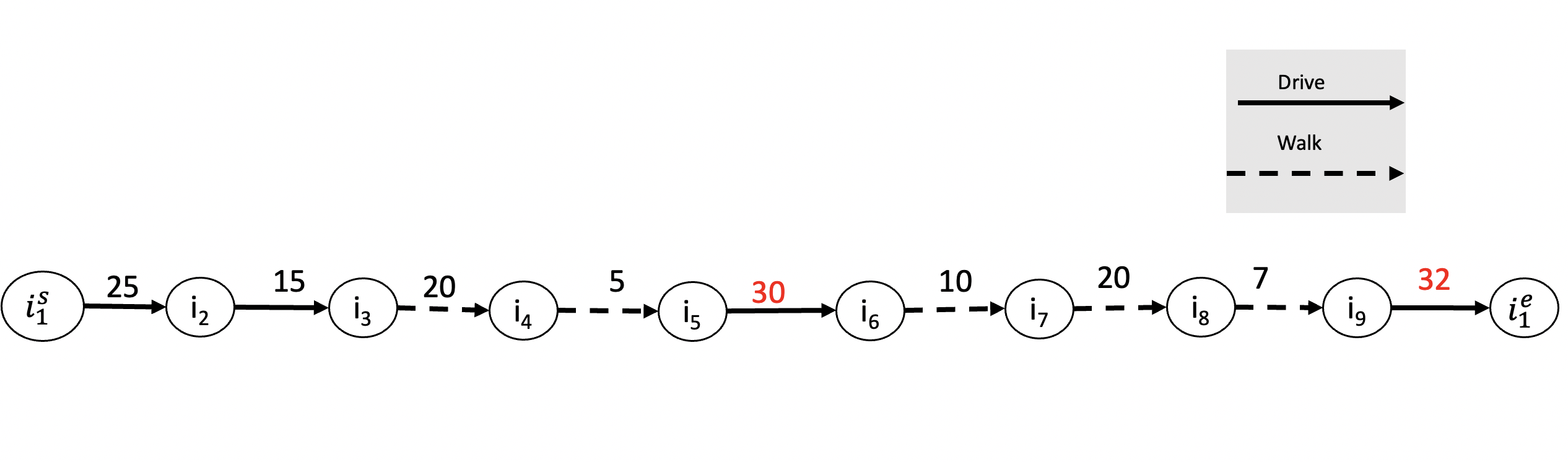
Figure 2: Graphical representation of solution encoding of itinerary of Figure 1. Red travel times refers to duration of walk-and-drive paths $(i_{5}-i_{3}-i_{6})$ and $(i_{9}-i_{6}-i^{e}_{1})$.

Given two PoIs $i$ and $k$ visited consecutively, we denote with $mode^{*}_{ik}$ the transport mode prescribed by $s^{\prime}_{*}$. We also denote with $t_{ik}$, the travel time needed to move from PoI $i$ to PoI $k$. If the prescribed transport mode is $Drive$, then the travel time $t_{ik}$ has to take properly into account the transfer time needed to switch from the pedestrian network to the road network at PoI $i$. In particular, a transfer connection starting at the origin PoI $i$ might generate a walking subtour. For example in the itinerary of Figure 1, in order to drive from PoI $i_{5}$ to PoI $i_{6}$, the tourist has to go on foot from PoI $i_{5}$ to PoI $i_{3}$ (transfer connection), pick up the vehicle parked nearby PoI $i_{3}$, drive from PoI $i_{3}$ to PoI $i_{6}$ and then park the vehicle nearby PoI $i_{6}$. In this case we have that $t_{i_{5}i_{6}}=t^{w}_{i_{5}i_{3}}+t^{d}_{i_{3}i_{6}}$. To evaluate in constant time the insertion of a new visit between PoIs $i_{5}$ and $i_{6}$, we need to encode also subtours. Firstly we maintain two quantities for the $h$-th subtour of an itinerary: the index of the first PoI and the index of the last PoI denote $FirstPoI_{h}$ and $LastPoI_{h}$, respectively. For example, the itinerary in Figure 1 has two subtours: the first subtour ($h=1$) is defined by the PoI sequence $i_{3}-i_{4}-i_{5}$ ($FirstPoI_{1}=i_{3},LastPoI_{1}=i_{5}$); the second subtour ($h=2$) is defined by the PoI sequence $i_{6}-i_{7}-i_{8}-i_{9}$ ($FirstPoI_{2}=i_{6},LastPoI_{2}=i_{9}$). We also maintain information for determining in constant time the subtour which a PoI belongs to. In particular, we denote with $S$ a vector of $|V|$ elements: if PoI $i$ belongs to subtour $h$, then $S_{i}=h$. For the example in Figure 1 we have that $S_{i_{3}}=S_{i_{4}}=S_{i_{5}}=1$, while $S_{i_{6}}=S_{i_{7}}=S_{i_{8}}=S_{i_{9}}=2$. To model that the remaining PoIs do not belong to any subtour we set $S_{i_{1}}=S_{i_{2}}=-1$. Given two PoIs $i$ and $k$ visited consecutively by solution $s^{\prime}_{*}$, the arrival time $a_{k}$ is determined as follows:

$$a_{k}=z_{i}+T_{i}+t_{ik},$$ (1)

where the travel time $t_{ik}$ is computed by Algorithm 3, according to the prescribed transport $mode$. If $S_{i}\neq-1$ and $mode=Drive$, then the input parameter $p$ denote the first PoI of the subtour which PoI $i$ belongs to, i.e. $p=FirstPoI_{S_{i}}$. If $mode=Walk$ the input parameter $p$ is set to a the deafult value $-1$. Parameter $Check$ is a boolean input, stating if soft constraints are relaxed or not. If $Check$ is $true$, when $mode_{ik}$ violates soft constraints the travel time $t_{ik}$ is set to a large positive value M, making the arrivals at later PoIs infeasible wrt (hard) time-window constraints. In all remaining cases $t_{ik}$ is computed according to the following relationship:

$$t_{ik}=t^{w}+t^{d}.$$ (2)

In particular if the prescribed transport mode is “walk from PoI $i$ to PoI $k$”, then $t^{w}=t^{w}_{ik}$ and $t^{d}=0$. Otherwise the prescribed transport mode is “walk from PoI $i$ to PoI $p$, pick-up the vehicle at PoI $p$ and then drive from PoI $p$ to PoI $k$”, with $t^{w}=t^{w}_{ip}$ and $t^{d}=t^{d}_{pk}$. We abuse notation and when PoI $i$ does not belong to a subtour ($S_{i}=-1$) and $mode=Drive$, we set $p=i$ with $t^{w}_{ii}=0$ and $mode_{ii}=Walk$. A further output of Algorithm 3 is the boolean value $Violated$, exploited during PoI insertion/removal to update the number of violated soft constraints.
The first six columns of Table 1 report the encoding of the itinerary reported in Figure 2. Tourist position is represented by dummy PoIs $i^{s}_{1}$ and $i^{e}_{1}$, with a visiting time equal to zero. The arrival time $a_{i}$ is computed according to (1). Column $z_{i}+T_{i}$ reports the leaving time with $z_{i}=max(a_{i},O_{i})$ and a visiting time $T_{i}$ equal to 5 time units. All leaving times satisfy time-window constraints, i.e. $z_{i}\leq C_{i}$. As far as the timing information associated to the starting and ending PoIs $i^{s}_{1}$ and $i^{e}_{1}$, they model that the tourist leaves $i^{s}_{1}$ at a given time instant (i.e. $a_{i^{s}_{1}}=0$), the itinerary duration is 224 time units, with time available for sightseeing equal 320 time units. All connections satisfy soft constraints, since we assume that $MaxWalkingTime$ and $MinDrivingTime$ are equal to 30 and 2 time units, respectively. The last four columns reports details about travel time computations performed by Algorithm 3. Travel time information between PoI $i$ and the next one is reported on the row associated to PoI $i$. Thus this data are not provided for the last (dummy) PoI $i^{e}_{1}$.

Table 1: Details of solution encoding for itinerary reported in Figure 2

Itinerary						Time windows		Travel Time Computation
PoI	Violated	$\textbf{mode}^{*}_{ik}$	$\textbf{S}_{i}$	$\textbf{a}_{i}$	$\textbf{z}_{i}\textbf{+T}_{i}$	$O_{i}$	$C_{i}$	p	$\textbf{t}^{w}$	$\textbf{t}^{d}$	$\textbf{t}_{ik}$
$i^{s}_{1}$	False	Drive	-1	0	0	0	0	$i^{s}_{1}$	0	25	25
$i_{2}$	False	Drive	-1	25	30	0	75	$i_{2}$	0	15	15
$i_{3}$	False	Walk	1	45	55	50	115	-1	20	0	20
$i_{4}$	False	Walk	1	75	80	60	95	-1	5	0	5
$i_{5}$	False	Drive	1	85	90	60	115	$i_{3}$	25	5	30
$i_{6}$	False	Walk	2	120	125	80	135	-1	10	0	10
$i_{7}$	False	Walk	2	135	155	150	175	-1	20	0	20
$i_{8}$	False	Walk	2	175	180	90	245	-1	7	0	7
$i_{9}$	False	Drive	2	187	192	90	245	$i_{6}$	27	5	32
$i^{e}_{1}$	-	-	-1	224	224	0	320	-	-	-	-

Data: M

Input: PoI $i$, PoI $k$, $mode$, $Check$, PoI $p$

Output: $t_{ik}$, Violated

1 Violated$\leftarrow$ False;

2 if $mode==Walk$ then

3      $t^{d}\leftarrow 0$;

4       if ($Check\wedge mode_{ik}\neq Walk$) then $t^{w}\leftarrow M$ else $t^{w}\leftarrow t^{w}_{ik}$;

5       if  ($mode_{ik}\neq Walk$) then Violated$\leftarrow$ True;

6      

7 else

8       if ($Check\wedge mode_{ip}\neq Walk$) then $t^{w}\leftarrow M$ else $t^{w}\leftarrow t^{w}_{ip}$;

9       if ($Check\wedge mode_{pk}\neq Drive$) then $t^{d}\leftarrow M$ else $t^{d}\leftarrow t^{d}_{pk}$;

10       if  ($mode_{ip}\neq Walk\vee mode_{pk}\neq Drive$) then Violated$\leftarrow$ True;

11      

12 $t_{ik}=t^{w}+t^{d}$;

Algorithm 3 Compute travel time

4.1 Feasibility check

In describing rules for feasibility checking, we will always consider inserting (unrouted) PoI $j$ between PoI $i$ and $k$. In the following we assume that PoI $j$ satisfies the max-n type constraints, modelling multiple time windows. Feasibility check rules are illustrated in the following by distinguishing three main insertion scenarios. The first one is referred to as basic insertion and assumes that the extra visit $j$ propagates a change only in terms of arrival times at later PoIs. The second one is referred to as advanced insertion and generates a change on later PoIs in terms of both arrival times and (extra) transfer time of subtour $S_{k}\neq-1$. The third one is referred to as a special case of the advanced insertion, with PoI $k$ not belonging to any subtour (i.e. $S_{k}$ is equal to -1). A special case insertion generates a new subtour where PoI $k$ is the last attraction to be visited.
Algorithm 4 reports the pseudocode of the feasibility check procedure, where the insertion type is determined by $(mode^{*}_{ik},S_{k},mode_{ij},mode_{jk})$. To illustrate the completeness of our feasibility check procedure, we report in Table 2 all insertion scenarios, discussed in detail in the following subsections. It is worth noting that if $mode^{*}_{ik}$ is $Walk$ then there exists a walking subtour consisting of at least PoIs $i$ and $k$, i.e. $S_{k}\neq-1$. For this reason we do not detail case 0 in Table 2.

Data: PoI $i$, PoI $j$,PoI $k$, incumbent solution $s^{*}$

1 Compute $Shift_{j}$ and $Wait_{j}$;

2 if $mode^{*}_{ik}=mode_{jk}\wedge(mode_{jk}=Drive\vee mode_{ij}=Walk)$ then

3       Check Feasibility with (5) and (6) // Basic Insertion;

4      

5else if $S_{k}\neq-1$ then

6       Compute $\Delta_{k}$ and $Shift_{q}$;

7       Check feasibility with (11), (12) and (6) // Advanced Insertion;

8      

9else

10      Compute $\Delta_{k}$ and $Shift_{q}$;

11       Check feasibility with (13), (12) and (6) // Special Case;

12      

13 end if

14

Algorithm 4 Feasibility check procedure

Table 2: Insertion scenarios and their relationships with feasibility check procedures.

Case	$mode^{*}_{ik}$	$S_{k}$	$(mode_{ij},mode_{jk})$	Insertion type
0	$Walk$	$=-1$	-	-
$1$	$Walk$	$\neq-1$	(Walk,Walk)	Basic
			(Drive,Drive)	Advanced
			(Walk,Drive)
			(Drive,Walk)
$2$	$Drive$	$\neq-1$	(Walk,Walk)	Advanced
			(Drive,Drive)	Basic
			(Walk,Drive)
			(Drive,Walk)	Advanced
$3$	$Drive$	$-1$	(Walk,Walk)	Special Case
			(Drive,Drive)	Basic
			(Walk,Drive)
			(Drive,Walk)	Special Case

4.1.1 Basic insertion

We observe that in a unimodal mobility environment a PoI insertion is always basic [17]. In a walk-and-drive mobility environment an insertion is checked as basic if one of the following conditions hold. If PoI $j$ is added to the walking subtour which PoI $i$ and PoI $j$ belong to, i.e. case 1 in Table 2 with $mode_{ij}=mode_{jk}=Walk$. In all other cases we have a basic insertion if it prescribes $Drive$ as transport mode from $j$ to $k$, i.e. case 1 and 2 with $mode_{jk}=Drive$. Five out of 12 scenarios of Table 2 refers to basic insertions. Conditions underlying the first three basic insertion scenarios is that $k$ belongs to a walking subtour (i.e. $S_{k}\neq-1$) and $FirstPoI_{S_{k}}$ is not updated after the insertion. The remaining basic insertions of Table 2 refer to scenarios where before and after the insertion, PoI $k$ does not belong to a subtour. All these five scenarios are referred to as basic insertions since the extra visit of PoI $j$ has an impact only on the arrival times at later PoIs.

Examples

To ease the discussion, we illustrate two examples of basic insertions for the itinerary of Figure 1. Other illustrative examples can be easily derived from Figure 1.

• Insert PoI $j$ between PoI $i=i_{3}$ and POI $k=i_{4}$, with $mode_{ij}=Walk$ and $mode_{jk}=Walk$. Before and after the insertion $FirstPoI_{S_{k}}$ is $i_{3}$ and, therefore, the insertion has no impact on later transfer connections.

• Insert PoI $j$ between Insert PoI $i=i^{s}_{1}$ and POI $k=i_{2}$, with $mode_{ij}=Walk$ and $mode_{jk}=Drive$. Before and after the insertion PoI $i_{2}$ does not belong to a subtour. Insertion can change only arrival times from PoI $i_{2}$ on.

To achieve an O(1) complexity for the feasibility check of a basic insertion, we adopt the approach proposed in [17] for a unimodal mobility environment and reported in the following for the sake of completeness. We define two quantities for each PoI $i$ selected by the incumbent solution: $Wait_{i}$, $MaxShift_{i}$. We denote with $Wait_{i}$ the waiting time occurring when the tourist arrives at PoI $i$ before the opening hour:

$$Wait_{i}=max\{0,O_{i}-a_{i}\}.$$

$MaxShift_{i}$ represents the maximum increase of start visiting time $z_{i}$, such that later PoIs can be visited before their closing hour. $MaxShift_{i}$ is defined by (3), where for notational convenience PoI $i+1$ represents the immediate successor of a generic PoI $i$.

$$MaxShift_{i}=min\{{\color[rgb]{0,0,0}C_{i}-z_{i}},Wait_{i+1}+MaxShift_{i+1}\}.$$ (3)

Table 3 reports values of $Wait$ and $MaxShift$ for the itinerary of Figure 1. It is worth noting that the definition of $MaxShift_{i}$ is a backward recursive formula, initialized with the difference ($C_{max}-z_{max}$), where $z_{max}$ denotes duration of the itinerary. To check the feasibility of an insertion of PoI $j$ between PoI $i$ and $k$, we compute extra time $Shift_{j}$ needed to reach and visit PoI $j$, as follows:

$$Shift_{j}=t_{ij}+Wait_{j}+T_{j}+t_{jk}-t_{ik}.$$ (4)

It is worth noting that travel times are computed by taking into account soft constraints (i.e. input parameter Check of Algorithm 3 is set equal to true). Feasibility of an insertion is checked in constant time at line 4 of Algorithm 4 by inequalities (5) and (6).

$$Shift_{j}=t_{ij}+Wait_{j}+T_{j}+t_{jk}-t_{ik}\leq Wait_{k}+MaxShift_{k}$$ (5)

$$z_{i}+T_{i}+t_{ij}+Wait_{j}\leq C_{j}.$$ (6)

4.1.2 Advanced insertion

In advanced insertion, the feasibility check has to take into account that the insertion has an impact on later PoIs in terms of both arrival times and transfer times. Let consider an insertion of a PoI $j$ between PoI $i_{2}$ and $i_{3}$ of Figure 1, with $mode_{i_{2}j}=mode_{ji_{3}}=Walk$. The insertion has an impact on the travel time from PoI $i_{5}$ to PoI $i_{6}$, i.e. after the insertion travel time $t_{i_{5}i_{6}}$ has to be updated to the new value $t^{new}_{i_{5}i_{6}}=t^{w}_{i_{5}i_{2}}+t^{d}_{i_{2}i_{6}}$. This implies that we have to handle two distinct feasibility checks. The former has a scope from PoI $i_{3}$ to $i_{5}$ and checks the arrival times with respect to $Shift_{j}$ computed according to (4). The latter concerns PoIs visited after $i_{5}$ and checks arrival times with respect to $Shift_{i_{5}}$, computed by taking into account both $Shift_{j}$ and the new value of $t_{i_{5}i_{6}}$. For notational convenience, the first PoI reached by driving after PoI $k$ is referred to as PoI $b$. Similarly, we denote with $q$ the last PoI of the walking subtour, which $k$ belongs to (i.e. if $S_{k}\neq-1$, then $q=LastPoI_{S_{k}}$). To check if the type of insertion is advanced, we have to answer the following question: has the insertion an impact on the travel time $t_{qb}$? To answer it is sufficient to check if after the insertion the value of $FirstPoI_{S_{k}}$ will be updated, i.e. the insertion changes the first PoI visited by the walking subtour $S_{k}$. Five out of 12 scenarios of Table 2 refers to advanced insertions, that is scenarios where $k$ belongs to a walking subtour (i.e. $S_{k}\neq-1$) and $FirstPoI_{S_{k}}$ is updated after the insertion. Algorithm 4 handles such advanced insertions by checking if one of the following conditions holds. The insertion of PoI $j$ splits the subtour which PoI $i$ and PoI $j$ belong to, i.e. case 1 in Table 2 with $mode_{ij}=Drive\vee mode_{jk}=Drive$. In all other cases the insertion is checked as advanced if PoI $j$ is appended at the beginning of the subtour $S_{k}$, i.e. case 2 in Table 2 with $mode_{jk}=Walk$.

Examples

As we did for basic insertions, we illustrate two advanced insertions for the itinerary of Figure 1. Other illustrative examples can be easily derived from Figure 1.

• Insert PoI $j$ between PoI $i=i_{7}$ and POI $k=i_{8}$, with $mode_{ij}=Drive$ and $mode_{jk}=Walk$. After the insertion $FirstPoI_{S_{k}}$ is $j$. Insertion change $t_{i_{9}i_{1}}$ to the new value $t^{new}_{i_{9}i_{1}}=t^{w}_{i_{9}j}+t^{d}_{ji_{1}}$.

• Insert PoI $j$ between PoI $i=i_{5}$ and POI $k=i_{6}$ , with $mode_{ij}=Walk$ and $mode_{jk}=Walk$. After the insertion $FirstPoI_{S_{k}}$ is $i_{3}$. Insertion change $t_{i_{9}i_{1}}$ to the new value $t^{new}_{i_{9}i_{1}}=t^{w}_{i_{9}i_{3}}+t^{d}_{i_{3}i_{1}}$.

To evaluate in constant time an advanced insertion, for each PoI $i$ included in solution $s^{\prime}_{*}$, three further quantities are defined when $S_{k}\neq-1$: $\overline{MaxShift}_{i}$, $\overline{Wait}_{i}$ and $ME_{i}$.
$\overline{MaxShift}_{i}$ represents the maximum increase of start visiting time $z_{i}$, such that later PoIs of subtour $S_{i}$ can be visited within their time windows. The definition of $\overline{MaxShift}_{i}$ is computed as follows in (backward) recursive manner starting with $\overline{MaxShift}_{q}=(C_{q}-z_{q})$.

$$\overline{MaxShift}_{i}=min\{{\color[rgb]{0,0,0}C_{i}-z_{i}},Wait_{i+1}+\overline{MaxShift}_{i+1}\}.$$ (7)

$\overline{Wait}_{i}$ corresponds to the sum of waiting times of later PoIs of subtour $S_{i}$. We abuse notation by denoting with $i+1$ the direct successor of PoI $i$ and such that $S_{i+1}=S_{i}$. Then we have that

$$\overline{Wait}_{i}=\overline{Wait}_{i+1}+Wait_{i},$$ (8)

with $\overline{Wait}_{LastPoI_{S_{i}}}=Wait_{LastPoI_{S_{i}}}$.
It worth recalling that in a multimodal mobility environment an insertion might propagate to later PoIs a decrease of the arrival times. The maximum decrease that a PoI $i$ can propagate is equal to $\max\{0,a_{i}-O_{i}\}$. $ME_{i}$ represents the maximum decrease of arrival times that can be propagated from PoI $i$ to $LastPoI_{S_{i}}$, that is

$$ME_{i}=\min\{ME_{i+1},\max\{(0,a_{i}-O_{i})\}\},$$ (9)

with $ME_{LastPoI_{S_{i}}}=\max\{(0,a_{LastPoI_{S_{i}}}-O_{LastPoI_{S_{i}}})\}$. If extra visit of PoI $j$ generates an increase of the arrival times at later PoIs, i.e. $Shift_{j}\geq 0$, then the arrival time of PoI $LastPoI_{S_{k}}$ is increased by the quantity $max\{0,Shift_{j}-\overline{Wait}_{k}\}$. On the other hand if $Shift_{j}<0$ then the arrival time of PoI $LastPoI_{S_{k}}$ is decreased by the quantity $\min\{ME_{k},|Shift_{j}|\}$. Let $\lambda_{j}$ be a boolean function stating when $Shift_{j}$ is non-negative:

$$\lambda_{j}=\left\{\begin{array}[]{rcl}1&&Shift_{j}\geq 0\\ 0&&Shift_{j}<0\\ \end{array}\right.$$

We quantify the impact of extra visit of PoI $j$ on the arrival times of PoI $LastPoI{S_{k}}$ by computing the value $\Delta_{k}$ as follows

$$\Delta_{k}=\lambda_{j}\times\max\{0,Shift_{j}-\overline{Wait}_{k}\}-(1-\lambda_{j})\times\min\{ME_{k},|Shift_{j}|\}.$$

To check the feasibility of the insertion of PoI $j$ between PoI $i$ and $k$, along with $Shift_{j}$ we compute $Shift_{q}$ as the difference between the new arrival time at PoI $b$ and the old one, that is:

$$Shift_{q}=t^{new}_{qb}+\Delta_{k}-t_{qb},$$ (10)

where $t^{new}_{qb}$ would be the new value of $t_{qb}$ if the algorithm inserted PoI $j$ between PoIs $i$ and $k$. Feasibility of the insertion of PoI $j$ between PoI $i$ and $k$ is checked in constant time at line 4 of Algorithm 4 by (11), (12) and (6).

$$Shift_{j}\leq Wait_{k}+\overline{MaxShift}_{k}$$ (11)

$$Shift_{q}\leq Wait_{b}+MaxShift_{b}.$$ (12)

Table 3 reports values of $\overline{Wait}$, $\overline{MaxShift}$ and $ME$ for subtours of itinerary of Figure 1. As we did for basic insertions, travel times are computed by taking into account soft constraints.

Special case

A special case of the advanced insertion is when PoI $k$ does not belong to a subtour (i.e. $S_{k}=-1$) in the solution $s^{\prime}_{*}$, but it becomes the last PoI of a new subtour after the insertion. Feasibility check rules (11) and (12) do not apply since $\overline{MaxShift}_{k}$, $\overline{Wait}_{k}$ and $ME_{k}$ are not defined. In this case, $\Delta_{k}$ is computed as follows:

$$\Delta_{k}=\lambda_{j}\max(0,Shift_{j}-Wait_{k})-(1-\lambda_{j})\min\{\max\{0,a_{k}-O_{k}\},|Shift_{j}|\}.$$

Then we set $q=k$ and compute $Shift_{q}$ according to (10). Feasibility of the insertion of PoI $j$ between PoI $i$ and $k$ is checked in constant time by (13), (12) and (6).

$$Shift_{j}\leq Wait_{k}+(C_{q}-z_{q}),$$ (13)

5 Updating an itinerary

During the local search after a PoI to be inserted has been selected and it has been decided where to insert the PoI, the affected itinerary needs to be updated. Similarly, during the perturbation phase after a set of selected PoIs has been removed, the affected itineraries need to be updated. The following subsections detail how we update the information maintained to facilitate feasibility checking when a PoI is inserted and a sequence of PoI is removed.

1 INIT: incumbent solution $s^{\prime}_{*}$;

2 for POI j visited by $s^{\prime}_{*}$ do

3       Determine the best feasible insertion with minimum value of $Shift^{\prime}_{j}$;

4       Compute $Ratio_{j}$;

5      

6 end for

7Select POI $j^{*}=arg\min\limits_{j}(Ratio_{j})$;

8 Visit $j^{*}$: Compute $a_{j^{*}}$, $z_{j^{*}}$, $Wait_{j^{*}}$, $Shift_{j^{*}}$, $S_{j^{*}}$;

9 Update information of subtours $S_{i^{*}}$, $S_{k^{*}}$;

10 if Advanced Insertion then $q^{*}\leftarrow LastPoI_{S_{k^{*}}}$, Compute $Shift_{q^{*}}$ else $q^{*}\leftarrow-1$;

11 $\overline{j}\leftarrow j^{*}$;

12 for POI j visited later than $j^{*}$ (Until $Shift_{j}=0$ $\wedge$ $j\geq q^{*}$) do // Forward Update

13       Update $a_{j}$, $z_{j}$, $Wait_{j}$,$S_{j}$;

14       if $j\neq q^{*}$ then Update $Shift_{j}$;

15       if $Shift_{j}=0$ $\wedge$ $j\geq q^{*}$ then $\overline{j}\leftarrow j$;

16      

17 end for

18for POI j visited earlier than $\overline{j}$ (Until $j=FirstPoI_{S_{j^{*}}}$)  do // Backward Update-Step 1

19       Update $MaxShift_{j}$;

20       if $S_{j}\neq-1$ then Update $\overline{Wait}_{j}$, $\overline{MaxShift}_{j}$, ${ME}_{j}$;

21      

22 end for

23for POI j visited earlier than $FirstPoI_{S_{i^{*}}}$ do // Backward Update-Step 2

24       Update $MaxShift_{j}$;

25      

26 end for

27Update the number of violated soft constraints;

28

Algorithm 5 Insertion Procedure

5.1 Insert and Update

Algorithm 5 reports the pseudocode of the proposed insertion procedure. During a major iteration of the local search, we select the best neighbour of the current solution $s^{\prime}_{*}$ as follows (Algorithm 5 lines 5-5). For each (unrouted) PoI $j$ we select the insertion with the minimum value of $Shift^{\prime}_{j}=Shift_{j}+Shift_{q}$. Then we compute $Ratio_{j}=(P_{j})^{2}/Shift^{\prime}_{j}$. The best neighbour is the solution obtained by inserting in $s^{\prime}_{*}$ the PoI $j^{*}$ with the maximum value of $Ratio_{j^{*}}$, i.e. $j^{*}=arg\max\limits_{j}{(P_{j})^{2}/Shift^{\prime}_{j}}$. Ties are broken by selecting the solution that best fits transport mode preferences, i.e. the insertion with the minimum number of violated soft constraints. The coordinate of the best insertion of $j^{*}$ are denoted with $i^{*}$, $k^{*}$. Solution is updated in order to include the visit of $j^{*}$ (Algorithm 5-lines 5-5). If the type of insertion is advanced we determine the value of $Shift_{q^{*}}$ according to (10) (Algorithm 5-line 5). Then, the solution encoding update consists of two consecutive main phases. The first phase is referred to as forward update, since it updates a few information related to visit of PoI $j^{*}$ and later PoIs. The forward update stops when the propagation of the insertion of $j^{*}$ has been completely absorbed by waiting times of later PoIs (Algorithm 5-lines 5-5). The second phase is initialized with the PoI $\overline{j}$ satisfying the stopping criterion of the forward update. Such final step is refereed to as backward update, since it iterates on PoIs visited earlier than $\overline{j}$ (Algorithm 5-lines 5-5). We finally update the number of violated constraints. As illustrated in the following, new arcs do not violate tourist preferences and therefore after the insertion of $j^{*}$ the number of violated soft constraints cannot increase.

Solution encoding update

Once inserted the new visit $j^{*}$ between PoI $i^{*}$ and PoI $k^{*}$, we update solution encoding as follows:

$$a_{j^{*}}=z_{i}^{*}+T_{i}^{*}+t_{i^{*}j^{*}}$$ (14)

$$Wait_{j^{*}}=\max\{0,O_{j^{*}}-a_{j^{*}}\}$$ (15)

$$Shift_{j^{*}}=t_{i^{*}j^{*}}+Wait_{j^{*}}+T_{j^{*}}+t_{j^{*}k^{*}}-t_{i^{*}k^{*}}.$$ (16)

If needed, we update $S_{j^{*}}$, $FirstPoI_{S_{k^{*}}}$ and $LastPoI_{S_{i}{{}^{*}}}$. The insertion of $j^{*}$ propagates a change of the arrival times at later PoIs only if $Shift_{j^{*}}\neq 0$. We recall that in a multimodal setting, the triangle inequality might not hold. This implies that $j^{*}$ insertion propagates either an increase (i.e. $Shift_{j^{*}}>0$) or a decrease (i.e. $Shift_{j^{*}}<0$) of the arrival times. Solution encoding of later PoIs is updated according to formula (17)-(20). For notational convenience we denote with $j$ the current PoI and $j-1$ its immediate predecessor.

$$a_{j}=a_{j}+Shift_{{j-1}}$$ (17)

$$Shift_{j}=\left\{\begin{array}[]{rcl}\max\{0,Shift_{{j-1}}-Wait_{j}\}&&Shift_{j-1}>0\\ \max\{O_{j}-z_{j},Shift_{j-1}\}&&Shift_{j-1}<0\\ \end{array}\right.$$ (18)

$$Wait_{j}=max\{0,O_{j}-a_{j}\}$$ (19)

$$z_{j}=z_{j}+Shift_{j}$$ (20)

At the first iteration, $j$ is initialized with $k^{*}$ and $Shift_{j-1}=Shift_{j^{*}}$. In particular (18) states that after $j$ it is propagated the portion of $Shift_{j-1}$ exceeding $Wait_{j}$, when $Shift_{j-1}>0$. Otherwise $Shift_{j}$ is strictly negative only if no waiting time occurs at PoI $j$ in solution $s^{\prime}_{*}$, that is $z_{j}>O_{j}$. If type of insertion is advanced we omit to update $Shift_{q^{*}}$, since it has been precomputed at line 5 according to (10). The forward updating procedure stops before the end of the itinerary if $Shift_{j}$ is zero, meaning that waiting times have entirely absorbed the initial increase/decrease of arrival times generated by $j^{*}$ insertion. Then we start the backward update, consisting of two main steps. During the first step the procedure iterates on PoIs visited between the POI $\overline{j}$, where the forward update stopped, and $FirstPoI_{S_{j}^{*}}$. We update $MaxShift_{j}$ according to the (3) as well as additional information for checking feasibility for advanced insertions. Therefore, if PoI $j$ belongs to a subtour (i.e. $S_{j}\neq-1$), then we also update $\overline{Wait_{j}}$, $\overline{MaxShift}_{j}$ and $ME_{j}$ according to the backward recursive formula (8), (7) and (9). The second step iterates on PoI $j$ visited earlier than $FirstPoI_{S_{j^{*}}}$ and updates only $MaxShift_{j}$.

5.2 Remove and Update

The perturbation procedure aims to remove for each itinerary of the incumbent solution $\rho_{d}$ PoIs visited consecutively starting from position $\sigma_{d}$. Given an itinerary, we denote with $i$ and $k$ respectively the last PoI and the first PoI, that are visited before and after the selected $\rho_{d}$ PoIs. Let $Shift_{i}$ denotes the variation of total travel time generated by the removal and propagated to PoIs visited later, that is:

$$Shift_{i}=t_{ik}-(a_{k}-T_{i}-z_{i}).$$

In particular when we compute $t_{ik}$ we do not take into account tourist preferences, i.e. in Algorithm 3 the input parameter $Check$ is equal to false. Due to multimodality, the triangle inequality might not be respected by the removal, since it can be propagate either an increase (i.e. $Shift_{i}>0$) or a decrease of the arrival times (i.e. $Shift_{i}<0$). In order to guarantee that after removing the selected PoIs, we obtain an itinerary feasible wrt hard constraints (i.e. time windows), we require that $Shift_{i}\leq 0$. To this aims we adjust the starting and the ending removal positions so that it is not allowed to remove portions of multiple subtours. In particular, if $S_{i}$ is not equal to $S_{k}$, then we set the initial and ending removal positions respectively to $FirstPOI_{S_{i}}$ and the immediate successor of $LastPOI_{S_{k}}$. In this way we remove subtours $S_{i}$, $S_{k}$ along with all the in-between subtours. For example in Figure 1, if $i$ and $k$ are equal to PoI $i_{2}$ and $i_{4}$ respectively, then we adjust $k$ so that the entire first subtour is removed, i.e. we set $k$ equal to $i_{6}$. Once the selected PoIs have been removed, the solution encoding update steps are the same of a basic insertion. We finally update the number of violated constraints.

1 INIT: an itinerary of solution $s^{\prime}_{*}$, i, k;

2 $mode=Drive$;

3 if $S_{i}=S_{k}$ then

4       if $S_{i}\neq-1$ then $mode\leftarrow Walk$;

5      

6 else

7       if $S_{i}\neq-1$ then $i\leftarrow FirstPoI_{S_{i}}$;

8       if $S_{k}\neq-1$ then $i\leftarrow$ immediate successor of $LastPoI_{S_{k}}$;

9      

10 end if

11Remove PoIs visited between $i$ and $k$;

12 $mode^{*}_{ik}=mode$;

13 $Shift_{i}\leftarrow t_{ik}-(a_{k}-z_{i}-T_{i})$;

14 Update $a_{i}$, $z_{i}$, $Wait_{i}$;

15 for POI j visited later than $i$ (Until $Shift_{j}=0$) do // Forward Update

16       Update $a_{j}$, $z_{j}$, $Wait_{j}$;

17       if $Shift_{j}=0$ then $\overline{j}\leftarrow j$;

18      

19 end for

20for POI j visited earlier than $\overline{j}$ (Until $j=i$)  do // Backward Update-Step 1

21       Update $MaxShift_{j}$;

22       if $S_{j}\neq-1$ then Update $\overline{Wait}_{j}$, $\overline{MaxShift}_{j}$, $ME_{j}$;

23      

24 end for

25Update $MaxShift_{i}$;

26 for POI j visited earlier than $i$ do // Backward Update-Step 2

27       Update $MaxShift_{j}$

28 end for

29

Algorithm 6 Perturbation Procedure

5.3 A numerical example

We provide a numerical example to illustrate the procedures described so far. We consider the itinerary of Figure 1.

In particular we illustrate the feasibility check of the following three insertions for a PoI $j$, with $[O_{j},C_{j}]=[0,300]$ and $T_{j}=5$. Durations of arcs involved in the insertion are reported in Figures 3 and Figure 4. As reported in Table 3 the itinerary of Figure 1 is feasible with respect to both time windows and soft constraints. As aforementioned, during the feasibility check, all travel times are computed by Algorithm 3 with input parameter $Check$ set equal to true.

Table 3: Solution encoding with additional information for itinerary of Figure 2

Itinerary						Time Windows		Additional data
PoI	Violated	$\textbf{mode}^{*}_{ik}$	$\textbf{S}_{i}$	$\textbf{a}_{i}$	$\textbf{z}_{i}\textbf{+T}_{i}$	$\textbf{O}_{i}$	$\textbf{C}_{i}$	$\textbf{Wait}_{i}$	$\textbf{MaxShift}_{i}$	$\overline{\textbf{Wait}_{i}}$	$\overline{\textbf{MaxShift}_{i}}$	$\textbf{ME}_{i}$
$i_{1}^{s}$	False	Drive	-1	0	0	0	0	0	0	-	-	-
$i_{2}$	False	Drive	-1	25	30	0	75	0	20	-	-	-
$i_{3}$	False	Walk	1	45	55	50	115	5	15	5	20	0
$i_{4}$	False	Walk	1	75	80	60	95	0	15	0	20	15
$i_{5}$	False	Drive	1	85	90	60	115	0	15	0	30	25
$i_{6}$	False	Walk	2	120	125	80	135	0	15	15	15	0
$i_{7}$	False	Walk	2	135	155	150	175	15	25	15	25	0
$i_{8}$	False	Walk	2	175	180	90	245	0	58	0	58	85
$i_{9}$	False	Drive	2	187	192	90	245	0	58	0	58	97
$i_{1}^{e}$	-	-	-1	224	224	0	320	0	96	-	-	-

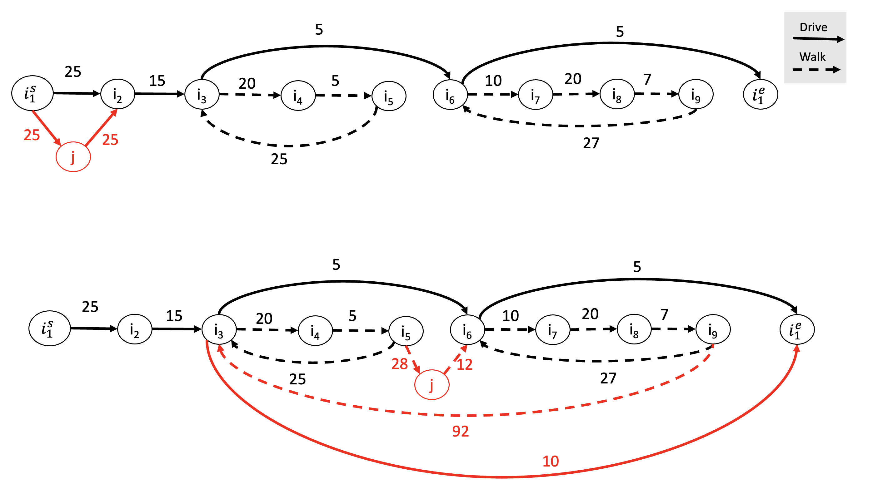
Figure 3: Example of infeasible insertions

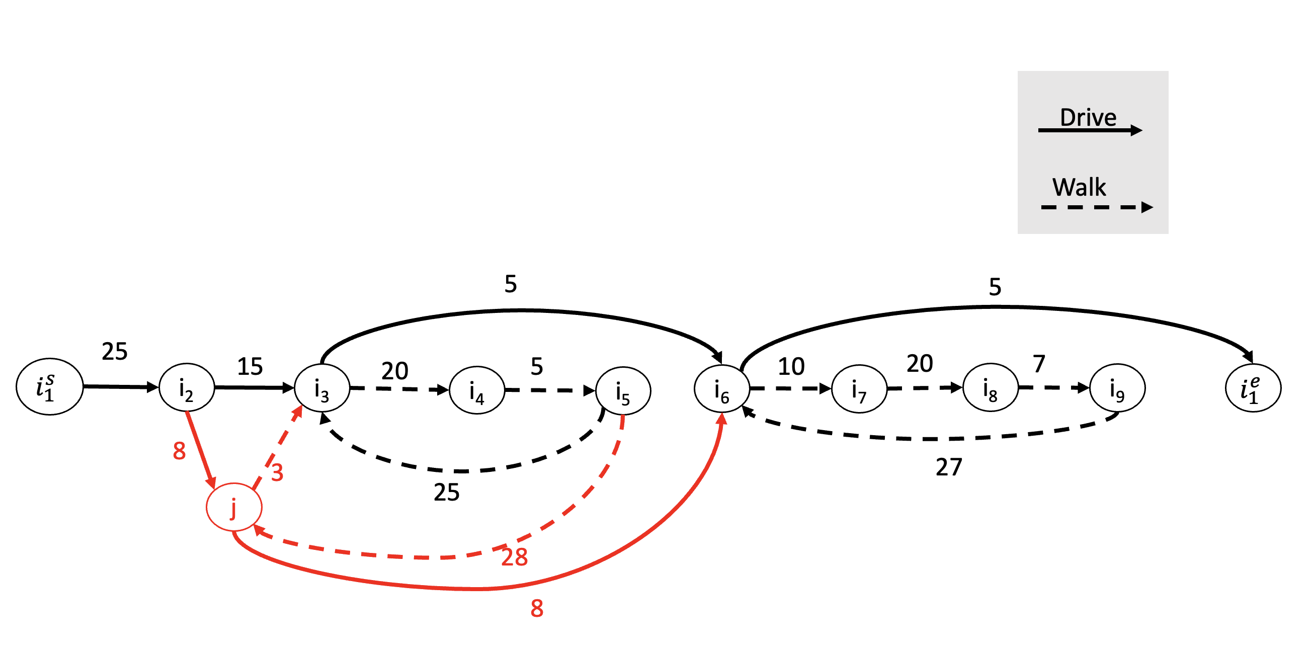
Figure 4: Example of feasible insertion

Insertion of PoI j between PoI $i^{s}_{1}$ and $i_{2}$ with $mode_{i_{1}j}=mode_{ji_{2}}=Drive$

We check feasibility by Algorithm 4, with $i=i^{s}_{1}$, $k=i_{2}$. The type of insertion is basic since $mode^{*}_{ik}=mode_{jk}$ and $mode_{jk}=Drive$. The feasibility is checked by (5) and (6), that is:

$$Shift_{j}=t_{ij}+Wait_{j}+T_{j}+t_{jk}-t_{ik}=25+0+5+25-25=30\nleq 0+20=Wait_{k}+MaxShift_{k},$$

$$z_{i}+T_{i}+t_{ij}+Wait_{j}=25\leq 80=C_{j},$$

where travel times $t_{ij}$ and $t_{jk}$ has been computed by Algorithm 3 with $p$ set equal to $i^{s}_{1}$ and $j$, respectively. The insertion violates time window of PoI $i_{4}$. Such infeasibility is checked through the violation of (5).

Insertion of PoI j between PoI $i_{5}$ and $i_{6}$ with $mode_{i_{5}j}=mode_{ji_{5}}=Walk$

We check feasibility by Algorithm 4, with $i=i_{5}$, $k=i_{6}$. The type of insertion is advanced since $mode^{*}_{ik}\neq mode_{jk}$ and $S_{k}\neq-1$. We recall that feasibility check consists of two parts. Firstly we check feasibility with respect to (11) and (6) that is

$$z_{i}+T_{i}+t_{ij}+Wait_{j}=118\leq 300=C_{j},$$

$$Shift_{j}=t_{ij}+Wait_{j}+T_{j}+t_{jk}-t_{ik}=15\leq 15=Wait_{k}+\overline{MaxShift}_{k},$$

where travel times have been computed by Algorithm 3, with $p=-1$. However the new visit of PoI $j$ is infeasible with respect to soft constraints. As aforementioned this case is encoded as a violation of time windows. Indeed, we compute $Shift_{q}$ according to (10) with $q=i_{9}$, $b=i^{e}_{1}$, where travel time $t^{new}_{qb}$ is computed by Algorithm 3, with $p=i_{3}$. Since the tourist has to walk more than 30 time units to pick up the vehicle, i.e. $t^{w}_{i_{9}i_{3}}=92$, then Algorithm 3 returns a value $t^{new}_{qb}$ equal to the (big) value M, which violates all time windows of later PoIs.

Insertion of PoI j between PoI $i_{2}$ and $i_{3}$ with $mode_{i_{2}j}=Drive$ and $mode_{ji_{3}}=Walk$

We check feasibility by Algorithm 4, with $i=i_{2}$, $k=i_{3}$. The type of insertion is advanced since $mode^{*}_{ik}\neq mode_{jk}$ and $S_{k}\neq-1$. The insertion does not violate time windows of PoI $j$ and PoIs belonging to the subtour $S_{k}$. This is checked by verifying that conditions (11) and (6) are satisfied, that is:

$$Shift_{j}=t_{ij}+Wait_{j}+T_{j}+t_{jk}-t_{ik}=1\leq 20=Wait_{k}+\overline{MaxShift}_{k},$$

$$z_{i}+T_{i}+t_{ij}+Wait_{j}=38\leq 300=C_{j},$$

where $t_{ij}$ and $t_{jk}$ are computed by Algorithm 3 with $p=-1$. Then we check feasibility with respect to closing hours of remaining (routed) PoIs. In particular we compute $Shift_{q}$ with $q=i_{5}$, $b=i_{6}$. Travel time $t^{new}_{qb}$ is computed with $p=j$. We have that $t^{new}_{qb}=28+8$. Since $Shift_{j}>0$, then $\Delta_{k}=\max\{0,Shift_{j}-\overline{Wait}_{k}\}=0$.

$$Shift_{q}=t^{new}_{qb}+\Delta_{k}-t_{qb}=36+0-30=6\leq 0+15=Wait_{b}+MaxShift_{b}.$$

The insertion is feasible since it satisfies also (12).
Table 4 shows details of the itinerary after the insertion of PoI $j$ between PoIs $i_{2}$ and $i_{3}$. It is worth noting that $Shift_{k}=0$, but the forward update stops at $\overline{j}=i_{7}$ since $Shift_{q}=6$. There is no need to update additional information of later PoIs.

Table 4: Details of the itinerary after the insertion

Itinerary						Time Windows		Additional data
PoI	Violated	$\textbf{mode}^{*}_{ik}$	$\textbf{S}_{i}$	$\textbf{a}_{i}$	$\textbf{z}_{i}\textbf{+T}_{i}$	$\textbf{O}_{i}$	$\textbf{C}_{i}$	$\textbf{Wait}_{i}$	$\textbf{MaxShift}_{i}$	$\overline{\textbf{Wait}_{i}}$	$\overline{\textbf{MaxShift}_{i}}$	$\textbf{ME}_{i}$
$i_{1}^{s}$	False	Drive	-1	0	0	0	0	0	0	-	-	-
$i_{2}$	False	Drive	-1	25	30	0	75	0	13	-	-	-
$j$	False	Walk	1	38	43	0	300	0	13	4	24	0
$i_{3}$	False	Walk	1	46	55	50	115	4	9	4	20	0
$i_{4}$	False	Walk	1	75	80	60	95	0	9	0	20	15
$i_{5}$	False	Drive	1	85	90	60	115	0	9	0	30	25
$i_{6}$	False	Walk	2	126	131	80	135	0	9	9	9	0
$i_{7}$	False	Walk	2	141	155	150	175	9	25	9	25	0
$i_{8}$	False	Walk	2	175	180	90	245	0	58	0	58	85
$i_{9}$	False	Drive	2	187	192	90	245	0	58	0	58	97
$i_{1}^{e}$	-	-	-1	224	224	0	320	0	96	-	-	-

Table 5: Details of the itinerary after the removal

Itinerary						Time Windows		Additional data
PoI	Violated	$\textbf{mode}^{*}_{ik}$	$\textbf{S}_{i}$	$\textbf{a}_{i}$	$\textbf{z}_{i}\textbf{+T}_{i}$	$\textbf{O}_{i}$	$\textbf{C}_{i}$	$\textbf{Wait}_{i}$	$\textbf{MaxShift}_{i}$	$\overline{\textbf{Wait}_{i}}$	$\overline{\textbf{MaxShift}_{i}}$	$\textbf{ME}_{i}$
$i_{1}^{s}$	False	Drive	-1	0	0	0	0	0	0	-	-	-
$i_{2}$	True	Drive	-1	25	30	0	75	0	50	-	-	-
$i_{6}$	False	Walk	2	32	85	80	135	48	55	103	55	0
$i_{7}$	False	Walk	2	95	155	150	175	55	25	55	25	0
$i_{8}$	False	Walk	2	175	180	90	245	0	58	0	58	85
$i_{9}$	False	Drive	2	187	192	90	245	0	58	0	58	97
$i_{1}^{e}$	-	-	-1	224	224	0	320	0	96	-	-	-

Removal of PoIs between $i_{2}$ and $i_{6}$

Table 5 reports details of the itinerary after the removal of PoIs visited between $i_{2}$ and $i_{6}$. Travel time $t_{i_{2}i_{6}}$ is computed by Algorithm 3 with input parameter $Check$ set equal to false. We observe that driving from PoI $i_{2}$ to PoI $i_{6}$ violates the soft constraint about $MinDrivingTime$, therefore after the removal the algorithm increases the total number of violated soft constraints.

6 Lifting ILS performance through unsupervised learning

The insertion heuristic explores in a systematic way the neighbourhood of the current solution. Of course, the larger the set $V$ the worse the ILS performance. In order to reduce the size of the neighbourhood explored by the local search, we exploited two mechanisms. Firstly, given the tourist starting position $i^{s}_{1}$, we consider an unrouted PoI as candidate for the insertion if it belongs to set:

$$\mathcal{N}_{r}(i^{s}_{1})=\{i\in V:d(i,i_{1}^{s})\leq r\}\subseteq V$$

where $d:V\times V\rightarrow\mathbb{R}^{+}$ denotes a non-negative distance function and the radius $r$ is a non negative scalar value. The main idea is that it is likely that the lowest ratio values are associated to PoIs located very far from $i^{s}_{1}$. We used the Haversine formula to approximate the shortest (orthodromic) distance between two geographical points along the Earth’s surface. The main drawback of this neighbourhood filtering is that a low value of radius $r$ might compromise the degree of diversification during the search. To overcome this drawback we adopt the strategy proposed in [51]. It is worth noting that in [51] test instances are defined on an Euclidean space. Since, we use a (more realistic) similarity measure representing the travel time duration of a quickest path, we cannot use k-means algorithm to build a clustering structure. To overcome this limitation we have chosen a hierarchical clustering algorithm. Therefore, during a preprocessing step we cluster PoIs. The adopted hierarchical clustering approach gives different partitioning depending on the level-of-resolution we are looking at. In particular, we exploited agglomerative clustering which is the most common type of hierarchical clustering. The algorithm starts by considering each observation as a single cluster; then, at each iteration two similar clusters are merged to define a new larger cluster until all observations are grouped into a single fat cluster. The result is a tree called dendrogram. The similarity between pair of clusters is established by a linkage criterion: e.g. the maximum distances between all observations of the two sets or the variance of the clusters being merged. In this work, the metric used to compute linkage is the walking travel time between pairs of PoIs in the mobility environment: this with the aim of reducing the total driving time. Given a PoI $i\in V$, we denote with $\mathcal{C}_{i}$ the cluster label assigned to $i$. $\mathcal{C}_{d}$ is the cluster containing the tourist starting position. We enhance the local search so that to ensure that a cluster (different from $\mathcal{C}_{d}$) is visited at most once in a tour. $\mathcal{C}_{d}$ can be visited at most twice in a tour: when departing from and when arriving to the depot, respectively. A PoI $j\in\mathcal{N}_{r}(i_{1}^{s})$ can be inserted between PoIs $i$ and $k$ in a itinerary $\mathfrak{p}$ only if at least one of the following conditions is satisfied:

• $\mathcal{C}_{i}=\mathcal{C}_{j}\vee\mathcal{C}_{k}=\mathcal{C}_{j}$, or

• $\mathcal{C}_{i}=\mathcal{C}_{k}=\mathcal{C}_{d}\wedge|\mathcal{L}_{\mathfrak{p}}|=1$, or

• $\mathcal{C}_{i}\neq\mathcal{C}_{k}\wedge\mathcal{C}_{j}\notin\mathcal{L}_{\mathfrak{p}}$,

where $\mathcal{L}_{\mathfrak{p}}$ denotes the set of all cluster labels for PoIs belonging to itinerary $\mathfrak{p}$. At first iteration of ILS $\mathcal{L}_{\mathfrak{p}}=\{\mathcal{C}_{d}\}$; subsequently, after each insertion of a PoI $j$, set $\mathcal{L}_{\mathfrak{p}}$ is enriched with $\mathcal{C}_{j}$. In the following section we thoroughly discuss about the remarkable performance improvement obtained, when such cluster based neighbourhood search is applied on (realistic) test instances with thousands of PoIs.

7 Computational experiments

This section presents the results of the computational experiments conducted to evaluate the performance of our method. We have tested our heuristic algorithm on a set of instances derived from the pedestrian and road networks of Apulia (Italy).

All experiments reported in this section were run on a standalone Linux machine with an Intel Core i7 processor composed by 4 cores clocked at 2.5 GHz and equipped with 16 GB of RAM. The machine learning component was implemented in Python (version 3.10). The agglomerative clustering implementations were taken from scikit-learn machine learning library. All other algorithms have been coded in Java.
Map data were extracted from OpenStreetMap (OSM) geographic database of the world (publicly available at https://www.openstreetmap.org). We used the GraphHopper (https://www.graphhopper.com/) routing engine to precompute all quickest paths between PoI pairs applying an ad-hoc parallel one-to-many Dijkstra for both moving modes (walking and driving). GraphHopper is able to assign a speed for every edge in the graph based on the road type extracted from OSM data for different vehicle profiles: on foot, hike, wheelchair, bike, racing bike, motorcycle and car. A fundamental assumption in our work is that travel times on both driving and pedestrian networks satisfy triangle inequality. In order to satisfy this preliminar requirement, we run the Floyd-Warshall [52, 53] algorithm as a post-processing step to enforce triangle inequality when not met (due to roundings or detours). The PoI-based graph consists of $3643$ PoIs. Walking speed has been fixed to $5$ km/h, while the maximum walking distance is $2.5$ km: i.e. the maximum time that can be traveled on foot is half an hour ($MaxWalkingTime$). As stated before, we improved the removal and insertion operators of the ILS proposed in order to take into account the extra travel time spent by the tourist to switch from the pedestrian network to the road network. Assuming that the destination has a parking service, we increased the traversal time by car of a customizable constant amount fixed to $10$ minutes ($ParkingTime$). We set the time need to switch from the pedestrian network to the road network equal to at least 5 time minutes ($PickUpTime$). Walking is the preferred mode whenever the traversal time by car is lower than or equal to $6$ minutes ($MinDrivingTime$). PoI score measures the popularity of attraction. We recall that the research presented in this paper is part of a project aiming to develop technologies enabling territorial marketing and tourism in Apulia (Italy). The popularity of PoIs has been extracted from a tourism related Twitter dataset presented in [54]. ILS is stopped after $150$ consecutive iterations without improvements or a time limit of one minute is reached.
Instances are defined by the following parameters:

• number of itineraries $m=1,2,3,4,5,6,7$;

• starting tourist position (i.e. its latitude and longitude);

• a radius $r=10,20,50,+\infty$ km for the spherical neighborhood $\mathcal{N}_{r}(i_{1}^{s})$ around the starting tourist position.

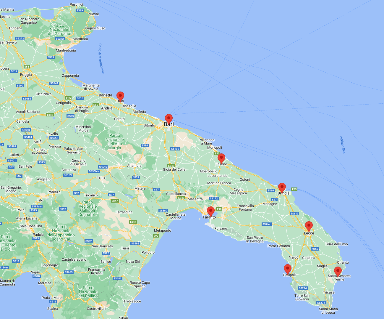
Figure 5: Starting positions.

We considered eight different starting positions along the Apulian territory, as showed in Figure 5. The maximum itinerary duration $C_{max}$ has been fixed to $12$ hours. Every PoI have $0$, $1$ or $2$ opening time-windows depending on current weekday.

Table 6: Candidate PoIs set size.

$r$	position	PoIs	$D_{1}$	$D_{2}$	$D_{3}$	$D_{4}$	$D_{5}$	$D_{6}$	$D_{7}$
10	1	172	257	257	257	203	257	256	148
	2	62	91	91	91	89	91	90	71
	3	172	214	215	176	216	216	136	137
	4	109	118	120	109	120	120	99	99
	5	118	127	132	122	132	132	109	108
	6	79	108	108	107	97	108	106	73
	7	117	140	141	115	141	141	140	140
	8	81	65	82	82	82	82	80	80
20	1	324	507	509	509	385	509	507	254
	2	117	174	172	174	169	174	174	129
	3	301	350	359	312	360	360	264	262
	4	245	266	280	251	280	280	223	222
	5	338	363	390	357	390	390	321	320
	6	262	359	359	346	305	359	354	228
	7	222	260	260	194	261	262	258	253
	8	263	296	329	328	287	329	324	240
50	1	872	1260	1289	1286	1009	1289	1279	712
	2	779	1010	1017	928	1008	1022	926	776
	3	1194	1380	1437	1306	1437	1441	1198	1130
	4	1267	1394	1463	1311	1463	1466	1202	1179
	5	1083	1185	1252	1124	1254	1254	994	991
	6	883	1232	1230	1147	1090	1235	1225	832
	7	836	1083	1082	938	1031	1089	1081	860
	8	670	875	905	902	768	905	896	606
$+\infty$	*	3643	4591	4570	4295	4521	4581	4297	3781

Table 6 summarizes for any radius-position pair:

• the number of PoIs in the spherical neighborhood $\mathcal{N}_{r}(i_{1}^{s})$;

• $D_{i}$ the number of PoIs opened during day $i$ ($i=1,\dots,m=7$, from Monday to Sunday).

When $r$ is set equal to $+\infty$ (last table line) no filter is applied and all $3643$ PoIs in the dataset are candidates for insertion.

Computational results are showed in Table 7, while Table 8 reports results obtained with PoI-clustering enabled. Each row represents the average value of the eight instances, with the following headings:

• DEV: the ratio between total score for the solution and the best known solution;

• TIME: execution time in seconds;

• PoIs: number of PoIs;

• $|S|$: number of walking subtours;

• SOL: number of improved solutions;

• IT: total number of iterations;

• IT_f: number of iterations without improvements w.r.t. the incumbent solution;

• $T^{d}$: total driving time divided by $m\cdot C_{max}$;

• $T^{w}$: total walking time divided by $m\cdot C_{max}$;

• $T$: total service time divided by $m\cdot C_{max}$;

• $W$: total waiting time divided by $m\cdot C_{max}$.

Since the territory is characterized by a high density of POIs, radius $r=50$ km is sufficient to build high-quality tours. Furthermore, we notice that the clustering-based ILS greatly improves the execution times of the algorithm, without compromising the quality of the final solution. In particular, the results obtained for increasing $m$ show that, when clustering is enabled, the ILS is able to do many more iterations, thus discovering new solutions and improving the quality of the final solution. When the radius value $r$ is lower than or equal to 50 Km and PoI-clustering is enabled, the algorithm stops mainly due to the iteration limit with $m$ not greater than $5$ itineraries.

The ILS approach is very efficient. The results confirm that the amount of time spent waiting is very small. Itineraries are well-composed with respect to total time spent travelling (without exhausting the tourist). On average, our approach builds itineraries with about $2$ walking subtours per day. In particular total walking time and total driving time corresponds respectively to about 6% and 20% of the available time. On average the visit time corresponds to about the 70% of the available time. Whilst the waiting time is on average less than 1.5%.

We further observe that by increasing the value $r$, the search execution times significantly increase with and without PoI-clustering. With respect to tour quality, clustered ILS is able to improve the degree of diversification on the territory, without remain trapped in high-profit isolated areas.

Table 7: Computational results

$m$	$r$	DEV [%]	TIME [s]	PoIs	$|S|$	SOL	IT	ITf	$T^{d}$ [%]	$T^{w}$ [%]	$T$ [%]	$W$ [%]
1	10	16.5	0.8	18.3	1.9	2.1	155.0	150.0	13.2	6.9	78.7	1.2
	20	9.3	1.7	19.4	2.5	2.4	157.3	150.0	17.0	7.4	74.9	0.7
	50	3.4	7.0	19.8	2.4	3.6	162.5	150.0	20.9	7.2	70.9	1.0
	$+\infty$	2.7	37.5	19.5	1.3	2.6	157.1	150.0	22.8	8.2	68.1	0.9
2	10	26.7	2.0	33.4	3.0	2.8	159.8	150.0	15.5	5.8	77.3	1.4
	20	16.8	5.3	35.0	5.1	4.5	165.8	150.0	19.5	6.0	73.2	1.3
	50	5.0	27.5	38.3	4.5	8.1	183.3	150.0	20.6	6.9	71.6	0.9
	$+\infty$	1.8	60.0	38.6	4.3	5.3	89.5	74.0	24.3	6.8	67.8	1.0
3	10	31.6	3.4	46.8	5.0	4.0	176.3	150.0	14.2	5.4	78.6	1.8
	20	19.2	10.0	50.8	7.1	5.1	170.8	150.0	19.6	5.7	73.4	1.3
	50	3.2	50.5	56.0	7.8	9.6	178.3	134.3	22.3	6.5	69.9	1.4
	$+\infty$	0.7	60.0	56.5	7.9	9.0	53.6	27.5	25.6	5.6	67.8	1.0
4	10	35.0	4.9	58.9	7.8	3.1	175.1	150.0	14.5	5.0	78.8	1.6
	20	21.7	16.0	65.5	9.5	7.1	190.1	150.0	20.1	5.1	73.2	1.5
	50	3.2	58.7	72.5	11.5	8.3	127.0	90.1	23.6	6.2	69.0	1.3
	$+\infty$	1.2	60.0	72.6	10.6	8.9	36.5	13.8	26.7	6.0	66.1	1.2
5	10	38.4	5.6	70.4	8.5	5.4	166.5	150.0	14.7	4.3	79.1	1.9
	20	24.4	25.4	78.8	11.3	6.3	197.5	150.0	19.6	5.0	73.7	1.7
	50	2.6	60.0	89.3	13.1	7.6	88.9	59.8	23.0	6.0	69.7	1.3
	$+\infty$	1.3	60.0	89.4	12.3	6.9	26.3	11.8	24.4	5.9	68.3	1.4
6	10	41.5	7.3	80.0	9.9	4.1	191.8	150.0	14.2	4.3	78.9	2.5
	20	27.2	27.6	90.8	13.9	5.6	184.6	150.0	20.4	4.8	73.0	1.8
	50	4.6	60.0	102.6	16.0	7.3	67.3	44.9	24.4	5.7	68.6	1.3
	$+\infty$	2.0	60.0	103.9	15.5	7.6	21.8	8.4	26.7	5.8	65.9	1.5
7	10	44.1	8.0	88.1	12.9	4.5	194.4	150.0	14.1	3.9	78.4	3.6
	20	28.4	34.3	104.5	15.0	6.0	180.1	150.0	19.5	4.9	73.5	2.2
	50	4.2	60.0	118.0	18.1	8.0	56.1	23.5	24.8	5.5	68.1	1.6
	$+\infty$	3.2	60.0	117.4	18.9	7.5	18.4	5.4	27.6	5.2	65.8	1.4
AVG		15.0	31.2	65.5	9.2	5.8	133.3	108.7	20.5	5.8	72.2	1.5

Table 8: Computational results with clustering

$m$	$r$	DEV [%]	TIME [s]	PoIs	$|S|$	SOL	IT	ITf	$T^{d}$ [%]	$T^{w}$ [%]	$T$ [%]	$W$ [%]
1	10	16.7	0.6	18.3	1.9	2.1	155.9	150.0	13.7	6.5	78.6	1.2
	20	9.7	0.9	19.4	2.4	2.8	157.3	150.0	16.5	6.9	75.7	0.8
	50	4.5	2.1	19.8	2.5	3.6	161.9	150.0	19.4	7.9	71.4	1.3
	$+\infty$	2.7	9.7	19.5	1.4	2.3	154.6	150.0	22.5	8.6	67.7	1.2
2	10	26.5	1.8	33.4	4.0	4.4	176.6	150.0	15.5	5.6	77.8	1.2
	20	16.8	2.5	35.4	4.3	3.3	164.8	150.0	18.0	6.8	73.6	1.6
	50	5.3	6.6	38.4	5.1	4.6	167.8	150.0	21.5	6.7	70.5	1.3
	$+\infty$	1.5	35.5	38.9	4.3	5.4	176.5	150.0	22.0	7.6	69.5	1.0
3	10	31.5	3.1	47.0	5.5	3.8	185.0	150.0	13.5	5.7	78.7	2.1
	20	19.2	4.9	51.3	7.1	4.4	192.0	150.0	19.2	5.8	73.5	1.5
	50	3.9	14.3	56.3	8.3	9.5	183.9	150.0	22.6	6.3	70.1	1.0
	$+\infty$	1.5	59.8	56.4	6.8	7.5	156.8	111.4	23.9	6.4	68.5	1.2
4	10	34.7	3.9	59.4	8.3	4.1	167.9	150.0	13.9	4.9	79.4	1.8
	20	22.0	7.6	64.9	9.1	5.1	191.6	150.0	19.8	5.3	73.3	1.6
	50	3.1	23.4	72.9	11.8	9.1	177.8	150.0	23.6	6.3	68.9	1.1
	$+\infty$	1.0	60.0	72.9	10.8	7.9	96.1	66.0	25.1	5.9	67.8	1.2
5	10	38.4	7.0	70.5	9.6	4.6	211.5	150.0	14.5	5.0	78.6	1.9
	20	24.7	10.0	78.9	10.6	5.1	187.9	150.0	19.3	5.2	73.9	1.6
	50	3.2	37.2	89.1	13.9	10.3	195.3	150.0	23.2	6.3	69.1	1.4
	$+\infty$	1.3	60.0	88.4	13.4	7.9	66.6	40.9	27.2	5.4	66.4	1.1
6	10	41.6	6.0	80.1	11.0	3.6	186.0	150.0	15.0	4.6	78.4	2.1
	20	27.1	14.0	91.5	12.6	6.5	212.8	150.0	19.9	5.1	72.9	2.1
	50	3.3	49.7	104.9	16.3	10.9	187.6	131.5	24.0	5.9	68.8	1.3
	$+\infty$	1.3	60.0	105.6	17.0	10.3	51.0	29.8	26.5	5.7	66.5	1.3
7	10	44.2	8.3	88.0	12.6	4.1	209.6	150.0	13.8	4.4	78.0	3.8
	20	28.4	14.4	104.3	16.6	4.8	169.3	150.0	19.5	4.7	73.8	2.0
	50	3.8	57.5	118.5	18.6	9.6	174.6	91.0	24.2	6.0	68.5	1.4
	$+\infty$	1.0	60.0	119.8	19.0	9.4	42.5	17.5	26.8	5.3	66.3	1.7
AVG		15.0	22.2	65.8	9.4	6.0	162.9	129.9	20.2	6.0	72.4	1.5

8 Conclusions

In this paper we have dealt with the tourist trip design problem in a walk-and-drive mobility environment, where the tourist moves from one attraction to the following one as a pedestrian or as a driver of a vehicle. Transport mode selection depends on the compromise between travel duration and tourist preferences. We have modelled the problem as a Team Orienteering Problem with multiple time windows on a multigraph, where tourist preferences on transport modes have been expressed as soft constraints.The proposed model is novel in the literature. We have also devised an adapted ILS coupled with an innovative approach to evaluate neighbourhoods in constant time. To validate our solution approach, realistic instances with thousands of PoIs have been tested. The proposed approach has succeeded in calculating personalised trips of up to 7 days in real-time. Future research lines will consider additional aspects, such as traffic congestion and PoI score dependency on visit duration.

References

- Gavalas et al. [2014a] Damianos Gavalas, Charalampos Konstantopoulos, Konstantinos Mastakas, and Grammati Pantziou. A survey on algorithmic approaches for solving tourist trip design problems. Journal of Heuristics, 20(3):291–328, 2014a.
- Ruiz-Meza and Montoya-Torres [2022] José Ruiz-Meza and Jairo R Montoya-Torres. A systematic literature review for the tourist trip design problem: extensions, solution techniques and future research lines. Operations Research Perspectives, page 100228, 2022.
- Ruiz-Meza and Montoya-Torres [2021] José Ruiz-Meza and Jairo R Montoya-Torres. Tourist trip design with heterogeneous preferences, transport mode selection and environmental considerations. Annals of Operations Research, 305(1):227–249, 2021.
- [4] 17 really useful things to know before visiting puglia. URL https://www.alongdustyroads.com/posts/useful-tips-puglia-italy.
- Li et al. [2020] Junxiong Li, Thi Hong Hai Nguyen, and J Andres Coca-Stefaniak. Coronavirus impacts on post-pandemic planned travel behaviours. Annals of Tourism Research, 2020.
- Gavalas et al. [2015a] D. Gavalas, C. Konstantopoulos, K. Mastakas, G. Pantziou, and N. Vathis. Heuristics for the time dependent team orienteering problem: Application to tourist route planning. Computers and Operations Research, 62:36–50, 2015a. ISSN 0305-0548. doi: https://doi.org/10.1016/j.cor.2015.03.016. URL https://www.sciencedirect.com/science/article/pii/S0305054815000817.
- Archetti et al. [2014] Claudia Archetti, M Grazia Speranza, and Daniele Vigo. Chapter 10: Vehicle routing problems with profits. In Vehicle routing: Problems, methods, and applications, second edition, pages 273–297. SIAM, 2014.
- Feillet et al. [2005] Dominique Feillet, Pierre Dejax, and Michel Gendreau. Traveling salesman problems with profits. Transportation science, 39(2):188–205, 2005.
- Dell’Amico et al. [1995] Mauro Dell’Amico, Francesco Maffioli, and Peter Värbrand. On prize-collecting tours and the asymmetric travelling salesman problem. International Transactions in Operational Research, 2(3):297–308, 1995.
- Archetti et al. [2009] Claudia Archetti, Dominique Feillet, Alain Hertz, and Maria Grazia Speranza. The capacitated team orienteering and profitable tour problems. Journal of the Operational Research Society, 60(6):831–842, 2009.
- Balas [1989] Egon Balas. The prize collecting traveling salesman problem. Networks, 19(6):621–636, 1989.
- Tang and Wang [2006] Lixin Tang and Xianpeng Wang. Iterated local search algorithm based on very large-scale neighborhood for prize-collecting vehicle routing problem. The International Journal of Advanced Manufacturing Technology, 29(11):1246–1258, 2006.
- Golden et al. [1987] Bruce L Golden, Larry Levy, and Rakesh Vohra. The orienteering problem. Naval Research Logistics (NRL), 34(3):307–318, 1987.
- Laporte and Martello [1990] Gilbert Laporte and Silvano Martello. The selective travelling salesman problem. Discrete applied mathematics, 26(2-3):193–207, 1990.
- Kataoka and Morito [1988] Seiji Kataoka and Susumu Morito. An algorithm for single constraint maximum collection problem. Journal of the Operations Research Society of Japan, 31(4):515–531, 1988.
- Chao et al. [1996] I-Ming Chao, Bruce L Golden, and Edward A Wasil. The team orienteering problem. European journal of operational research, 88(3):464–474, 1996.
- Vansteenwegen et al. [2009] Pieter Vansteenwegen, Wouter Souffriau, Greet Vanden Berghe, and Dirk Van Oudheusden. Iterated local search for the team orienteering problem with time windows. Computers & Operations Research, 36(12):3281–3290, 2009.
- Boussier et al. [2007] Sylvain Boussier, Dominique Feillet, and Michel Gendreau. An exact algorithm for team orienteering problems. 4or, 5(3):211–230, 2007.
- Righini and Salani [2009] Giovanni Righini and Matteo Salani. Decremental state space relaxation strategies and initialization heuristics for solving the orienteering problem with time windows with dynamic programming. Computers & Operations Research, 36(4):1191–1203, 2009. ISSN 0305-0548. doi: https://doi.org/10.1016/j.cor.2008.01.003. URL https://www.sciencedirect.com/science/article/pii/S030505480800004X.
- Montemanni et al. [2011] R. Montemanni, D. Weyland, and L.M. Gambardella. An enhanced ant colony system for the team orienteering problem with time windows. In 2011 International Symposium on Computer Science and Society, pages 381–384, 2011. doi: 10.1109/ISCCS.2011.95.
- Tricoire et al. [2010] Fabien Tricoire, Martin Romauch, Karl F Doerner, and Richard F Hartl. Heuristics for the multi-period orienteering problem with multiple time windows. Computers & Operations Research, 37(2):351–367, 2010.
- Zografos and Androutsopoulos [2008] Konstantinos G Zografos and Konstantinos N Androutsopoulos. Algorithms for itinerary planning in multimodal transportation networks. IEEE Transactions on Intelligent Transportation Systems, 9(1):175–184, 2008.
- Garcia et al. [2013] Ander Garcia, Pieter Vansteenwegen, Olatz Arbelaitz, Wouter Souffriau, and Maria Teresa Linaza. Integrating public transportation in personalised electronic tourist guides. Computers & Operations Research, 40(3):758–774, 2013.
- Gavalas et al. [2015b] Damianos Gavalas, Charalampos Konstantopoulos, Konstantinos Mastakas, Grammati Pantziou, and Nikolaos Vathis. Heuristics for the time dependent team orienteering problem: Application to tourist route planning. Computers & Operations Research, 62:36–50, 2015b.
- Ruiz-Meza et al. [2021a] José Ruiz-Meza, Julio Brito, and Jairo R. Montoya-Torres. A grasp to solve the multi-constraints multi-modal team orienteering problem with time windows for groups with heterogeneous preferences. Computers & Industrial Engineering, 162:107776, 2021a. ISSN 0360-8352. doi: https://doi.org/10.1016/j.cie.2021.107776. URL https://www.sciencedirect.com/science/article/pii/S036083522100680X.
- Yu et al. [2017] Vincent F. Yu, Parida Jewpanya, Ching-Jung Ting, and A.A.N. Perwira Redi. Two-level particle swarm optimization for the multi-modal team orienteering problem with time windows. Applied Soft Computing, 61:1022–1040, 2017. ISSN 1568-4946. doi: https://doi.org/10.1016/j.asoc.2017.09.004. URL https://www.sciencedirect.com/science/article/pii/S1568494617305434.
- Vansteenwegen and Gunawan [2019] Pieter Vansteenwegen and Aldy Gunawan. Orienteering problems. EURO Advanced Tutorials on Operational Research, 2019.
- Yu et al. [2019] Qinxiao Yu, Kan Fang, Ning Zhu, and Shoufeng Ma. A matheuristic approach to the orienteering problem with service time dependent profits. European Journal of Operational Research, 273(2):488–503, 2019. ISSN 0377-2217. doi: https://doi.org/10.1016/j.ejor.2018.08.007. URL https://www.sciencedirect.com/science/article/pii/S0377221718306842.
- Gündling and Witzel [2020] Felix Gündling and Tim Witzel. Time-dependent tourist tour planning with adjustable profits. In 20th Symposium on Algorithmic Approaches for Transportation Modelling, Optimization, and Systems (ATMOS 2020). Schloss Dagstuhl-Leibniz-Zentrum für Informatik, 2020.
- Khodadadian et al. [2022] M. Khodadadian, A. Divsalar, C. Verbeeck, A. Gunawan, and P. Vansteenwegen. Time dependent orienteering problem with time windows and service time dependent profits. Computers & Operations Research, 143:105794, 2022. ISSN 0305-0548. doi: https://doi.org/10.1016/j.cor.2022.105794. URL https://www.sciencedirect.com/science/article/pii/S0305054822000831.
- Verbeeck et al. [2014] C. Verbeeck, P. Vansteenwegen, and E.-H. Aghezzaf. An extension of the arc orienteering problem and its application to cycle trip planning. Transportation Research Part E: Logistics and Transportation Review, 68:64–78, 2014. ISSN 1366-5545. doi: https://doi.org/10.1016/j.tre.2014.05.006. URL https://www.sciencedirect.com/science/article/pii/S1366554514000751.
- Zheng and Liao [2019] Weimin Zheng and Zhixue Liao. Using a heuristic approach to design personalized tour routes for heterogeneous tourist groups. Tourism Management, 72:313–325, 2019.
- Ruiz-Meza et al. [2021b] José Ruiz-Meza, Julio Brito, and Jairo R Montoya-Torres. A grasp to solve the multi-constraints multi-modal team orienteering problem with time windows for groups with heterogeneous preferences. Computers & Industrial Engineering, 162:107776, 2021b.
- Zheng et al. [2020] Weimin Zheng, Haipeng Ji, Congren Lin, Wenhui Wang, and Bilian Yu. Using a heuristic approach to design personalized urban tourism itineraries with hotel selection. Tourism Management, 76:103956, 2020.
- Divsalar et al. [2013] A. Divsalar, P. Vansteenwegen, and D. Cattrysse. A variable neighborhood search method for the orienteering problem with hotel selection. International Journal of Production Economics, 145(1):150–160, 2013. ISSN 0925-5273. doi: https://doi.org/10.1016/j.ijpe.2013.01.010. URL https://www.sciencedirect.com/science/article/pii/S0925527313000285.
- Expósito et al. [2019a] Airam Expósito, Simona Mancini, Julio Brito, and José A Moreno. Solving a fuzzy tourist trip design problem with clustered points of interest. In Uncertainty management with fuzzy and rough sets, pages 31–47. Springer, 2019a.
- Expósito et al. [2019b] Airam Expósito, Simona Mancini, Julio Brito, and José A. Moreno. A fuzzy grasp for the tourist trip design with clustered pois. Expert Systems with Applications, 127:210–227, 2019b. ISSN 0957-4174. doi: https://doi.org/10.1016/j.eswa.2019.03.004. URL https://www.sciencedirect.com/science/article/pii/S0957417419301575.
- Gavalas et al. [2015c] Damianos Gavalas, Vlasios Kasapakis, Charalampos Konstantopoulos, Grammati Pantziou, Nikolaos Vathis, and Christos Zaroliagis. The ecompass multimodal tourist tour planner. Expert systems with Applications, 42(21):7303–7316, 2015c.
- Souffriau et al. [2013a] Wouter Souffriau, Pieter Vansteenwegen, Greet Vanden Berghe, and Dirk Van Oudheusden. The multiconstraint team orienteering problem with multiple time windows. Transportation Science, 47(1):53–63, 2013a. doi: 10.1287/trsc.1110.0377.
- Amarouche et al. [2020] Youcef Amarouche, Rym Nesrine Guibadj, Elhadja Chaalal, and Aziz Moukrim. Effective neighborhood search with optimal splitting and adaptive memory for the team orienteering problem with time windows. Computers & Operations Research, 123:105039, 2020.
- Karabulut and Tasgetiren [2020] Korhan Karabulut and M Fatih Tasgetiren. An evolution strategy approach to the team orienteering problem with time windows. Computers & Industrial Engineering, 139:106109, 2020.
- Tang and Miller-Hooks [2005] Hao Tang and Elise Miller-Hooks. A tabu search heuristic for the team orienteering problem. Computers & Operations Research, 32(6):1379–1407, 2005. ISSN 0305-0548. doi: https://doi.org/10.1016/j.cor.2003.11.008. URL https://www.sciencedirect.com/science/article/pii/S0305054803003265.
- Lin and Yu [2012] Shih-Wei Lin and Vincent F. Yu. A simulated annealing heuristic for the team orienteering problem with time windows. European Journal of Operational Research, 217(1):94–107, 2012. ISSN 0377-2217. doi: https://doi.org/10.1016/j.ejor.2011.08.024. URL https://www.sciencedirect.com/science/article/pii/S037722171100765X.
- Lin and Yu [2015] Shih-Wei Lin and Vincent F. Yu. A simulated annealing heuristic for the multiconstraint team orienteering problem with multiple time windows. Applied Soft Computing, 37:632–642, 2015. ISSN 1568-4946. doi: https://doi.org/10.1016/j.asoc.2015.08.058. URL https://www.sciencedirect.com/science/article/pii/S1568494615005712.
- Dang et al. [2013] Duc-Cuong Dang, Rym Nesrine Guibadj, and Aziz Moukrim. An effective pso-inspired algorithm for the team orienteering problem. European Journal of Operational Research, 229(2):332–344, 2013. ISSN 0377-2217. doi: https://doi.org/10.1016/j.ejor.2013.02.049. URL https://www.sciencedirect.com/science/article/pii/S0377221713001987.
- Ke et al. [2008] Liangjun Ke, Claudia Archetti, and Zuren Feng. Ants can solve the team orienteering problem. Computers & Industrial Engineering, 54(3):648–665, 2008. ISSN 0360-8352. doi: https://doi.org/10.1016/j.cie.2007.10.001. URL https://www.sciencedirect.com/science/article/pii/S0360835207002161.
- Hamid et al. [2021] Rula A. Hamid, A.S. Albahri, Jwan K. Alwan, Z.T. Al-qaysi, O.S. Albahri, A.A. Zaidan, Alhamzah Alnoor, A.H. Alamoodi, and B.B. Zaidan. How smart is e-tourism? a systematic review of smart tourism recommendation system applying data management. Computer Science Review, 39:100337, 2021. ISSN 1574-0137. doi: https://doi.org/10.1016/j.cosrev.2020.100337. URL https://www.sciencedirect.com/science/article/pii/S1574013720304378.
- Gavalas et al. [2014b] Damianos Gavalas, Charalampos Konstantopoulos, Konstantinos Mastakas, and Grammati Pantziou. Mobile recommender systems in tourism. Journal of Network and Computer Applications, 39:319–333, 2014b. ISSN 1084-8045. doi: https://doi.org/10.1016/j.jnca.2013.04.006. URL https://www.sciencedirect.com/science/article/pii/S1084804513001094.
- Borràs et al. [2014] Joan Borràs, Antonio Moreno, and Aida Valls. Intelligent tourism recommender systems: A survey. Expert systems with applications, 41(16):7370–7389, 2014.
- Souffriau et al. [2013b] Wouter Souffriau, Pieter Vansteenwegen, Greet Vanden Berghe, and Dirk Van Oudheusden. The multiconstraint team orienteering problem with multiple time windows. Transportation Science, 47(1):53–63, 2013b.
- Gavalas et al. [2013] Damianos Gavalas, Charalampos Konstantopoulos, Konstantinos Mastakas, Grammati Pantziou, and Yiannis Tasoulas. Cluster-based heuristics for the team orienteering problem with time windows. In International Symposium on Experimental Algorithms, pages 390–401. Springer, 2013.
- Floyd [1962] Robert W Floyd. Algorithm 97: shortest path. Communications of the ACM, 5(6):345, 1962.
- Warshall [1962] Stephen Warshall. A theorem on boolean matrices. Journal of the ACM (JACM), 9(1):11–12, 1962.
- Stirparo et al. [2022] Davide Stirparo, Beatrice Penna, Mohammad Kazemi, and Ariona Shashaj. Mining tourism experience on twitter: A case study, 2022. URL https://arxiv.org/abs/2207.00816.