End-to-end Learning for Image-based Detection of Molecular Alterations in Digital Pathology

Abstract

Current approaches for classification of whole slide images (WSI) in digital pathology predominantly utilize a two-stage learning pipeline. The first stage identifies areas of interest (e.g. tumor tissue), while the second stage processes cropped tiles from these areas in a supervised fashion. During inference, a large number of tiles are combined into a unified prediction for the entire slide. A major drawback of such approaches is the requirement for task-specific auxiliary labels which are not acquired in clinical routine.

We propose a novel learning pipeline for WSI classification that is trainable end-to-end and does not require any auxiliary annotations. We apply our approach to predict molecular alterations for a number of different use-cases, including detection of microsatellite instability in colorectal tumors and prediction of specific mutations for colon, lung, and breast cancer cases from The Cancer Genome Atlas. Results reach AUC scores of up to 94% and are shown to be competitive with state of the art two-stage pipelines. We believe our approach can facilitate future research in digital pathology and contribute to solve a large range of problems around the prediction of cancer phenotypes, hopefully enabling personalized therapies for more patients in future.

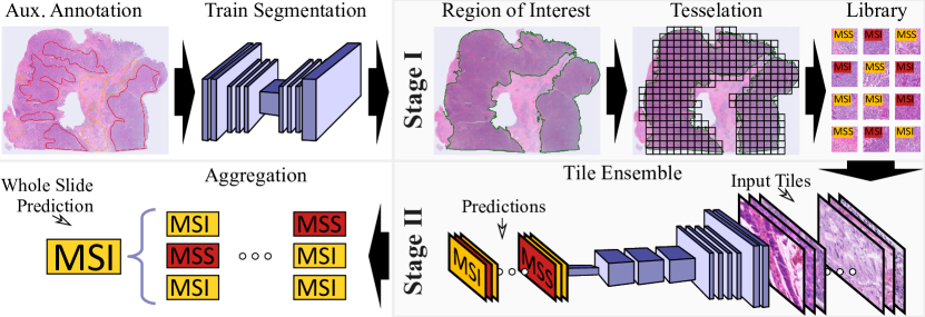
Figure 1: Visualization of a typical two stage pipeline.

As Whole Slide Imaging (WSI) is becoming a common modality in digital pathology, large numbers of highly-resolved microscopic images are readily available for analysis. Meanwhile, precision medicine allows for a targeted therapy of more and more cancer types, making the detection of actionable genetic alterations increasingly valuable for treatment planning and prognosis. Over the last few years, several studies have focused on the prediction of specific mutations, molecular subgroups or patient outcome from microscopy data of tumor tissue [5, 3, 11]. The large size of WSI images and the localized nature of information have led to the development of specific processing pipelines for this application.

In a comprehensive review, Echele et al. [5] observe that the majority of work on WSI classification comprises two stages. Depending on the task at hand, the first stage selects a region of interest (ROI) of a certain type of tissue or high tumor content [11, 4, 14], while some tasks [20, 29] and methods [7, 21] require even more detailed localized annotation. This stage typically involves a separately trained segmentation model. In the second stage, tessellation of the ROI creates a set of smaller tiles (e.g. $224\times 244$ pixels) that are well suited for processing with convolution neural networks (CNNs). For training, each tile is assigned the same target label corresponding to the whole slide. During inference, a subset or all of the tiles from a ROI are classified by the CNN. In order to obtain a slide-level prediction, all tile-level predictions are combined, e.g. by averaging the confidences [11], class voting [3] or by a second-level classifier [20]. We visualize a typical two-stage pipeline in Figure 1. Some studies [5, 13] omit the segmentation step and randomly choose tiles across the entire slide. This adds label noise to the classification step, since some areas (e.g. healthy tissue) do not contain any relevant information for the classification task at hand, which decreases the prediction performance.

Recently, a few works which avoid auxiliary annotations have been presented. Weakly supervised methods aim to implicitly identify tiles with high information value without manual annotation [1, 2, 9]. In another line of work, clustering-based methods have been proposed for end-to-end WSI classification [17, 25, 26]. A recent benchmark [13] compares a number of state-of-the-art weakly supervised and end-to-end training methods for WSI classification. Their results indicate that the known weakly supervised and end-to-end methods are unable to outperform the widely used two-stage prediction pipeline. The existing methods therefore effectively trade annotation effort for prediction performance.

In this paper, we introduce a $k$-Siamese CNN architecture for WSI classification which is trainable end-to-end, does not require any auxiliary annotations, and is straight-forward to implement. We show that our method outperforms a reference two-stage approach in the clinically relevant task of microsatellite instability (MSI) classification in WSI of formalin-fixed paraffin-embedded (FFPE) slides with haematoxylin and eosin (H&E) stained tissue samples of colorectal cancer. In addition, we present competitive results on multiple tasks derived from a range of molecular alterations for breast, colon and lung cancer on the public Cancer Genome Atlas database (TCGA).

1 Our Method: $k$-Siamese Networks

We believe that the main reason for the success of two-stage approaches is that they mitigate the label noise issue inherent to tile based processing. Training a classifier on every tile from a WSI separately is disadvantageous since a large number of tiles do not contain any visual clues on the task at hand. Tiles showing only healthy tissue for example do not contain any information about the tumor. We know that CNNs are able to overfit most datasets, if this is the optimal strategy to minimize training error [31]. Utilizing uninformative tiles during training therefore results in the network learning features which degrade its generalization ability. We believe that this is the main reason that led to two-stage approaches becoming so popular for WSI analysis. However, for some tasks only a subset of the tumor area might contain the relevant information, for other tasks it might be required to combine visual information from multiple tiles before taking a decision. Both scenarios are not handled well by current two-stage pipelines.

We propose a novel encoder-decoder based pipeline to address these issues. Our encoder produces a latent representation for $k$ randomly selected tiles from the input WSI. These tiles are processed simultaneously while sharing their weights. The resulting set of feature vectors is than aggregated by the decoder to output a single joined prediction. We call our approach $k$-Siamese networks, since it follows the idea of Siamese networks, but with $k$ instead of just two encoders. We illustrate our approach in Figure 2.

The feature vectors produced by the encoder are learned implicitly and can store any kind of information, including that the tile is not meaningful for the task at hand. The decoder can learn to interpret those feature vectors and combine the information found in multiple tiles. If $k$ is chosen large enough, a sufficient number of the selected tiles contain task-relevant information, which eliminates the need for any auxiliary annotations.

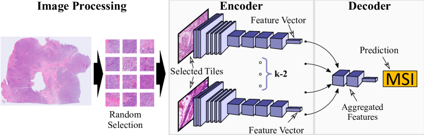
Figure 2: An overview over our end-to-end learning pipeline.

1.0.1 Design Choices

Our encoder is based on Efficientnet-B0 [30], which offers high predictive capability with a relatively small computational and memory footprint. Our decoder performs average pooling over the feature vectors from all $k$ patches, followed by a $1\times 1$ convolution and a softmax layer. We have evaluated more complex designs however, we did not observe any significant performance boost. Utilizing adaptive average pooling for the feature vector aggregation step has the additional benefit that the model can be used with a variable number of encoders. This allows us to perform memory efficient training with as few as $24$ tiles, while using more tiles for better prediction performance during inference.

1.0.2 Training and Inference

Our model is trained with stochastic gradient-descent using the Adam heuristic [12]. For training the encoder, we use a fine-tuning approach and start with the official EfficientNet weights, provided Tan et al. [30]. Unless otherwise specified, we use the following training parameters for all our experiments: base learning-rate ($blr$) of $2\text{\times}{10}^{-5}$ and batch-size ($bs$) of $6$.

Following the discussions in [8], we normalize our learning-rate ($nlr$) by multiplying the base-learning rate ($blr$) with our batch-size ($bs$): $nlr=bs\times blr$. We train the model for $72$ epochs and report the scores evaluated on the final epoch. We use $12$ warm-up epochs, during which the learning rate ($lr$) is linearly increased from $0$ to $nlr$ [8]. For the remaining $60$ epochs, we use polynomial learning rate decay [16]. We use automatic mixed precision (amp) [19] training to reduce the memory and computational footprint. To improve generalization, we use the following regularization methods: We apply quadratic weight decay with a factor of $5\text{\times}{10}^{-4}$ to all our weights. We use dropout [28] for the decoder and stochastic depth [10] for the encoder. We apply data-augmentation to each tile independently. We use the following common data-augmentation methods: (random) brightness, contrast, saturation, hue and rotation. In addition, tiles are not taken from a fixed grid, but their location is chosen randomly but non-overlapping. We exclude tiles which only contain background, which is estimated by using a threshold on the colour values.

During training, we use $24$ tiles per slide, each with a spatial resolution of $256\times 256$ pixel. We perform inference on $96$ tiles. All tiles have an isometric resolution of $0.25$ microns/pixel, which corresponds to a $10\times$ optical magnification.

2 Data

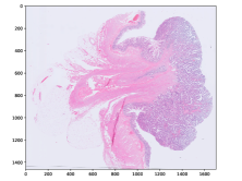
(a) MSI negative

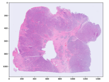
(b) MSI positive

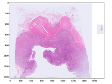
(c) MSI negative

Figure 3: Three examples of diagnostic slides from the CancerScout Colon dataset. Slides are plotted with an optical magnification of 2.5.

2.1 The CancerScout Colon Data

For this study, we use $2085$ diagnostic slides from $840$ colon cancer patients. We have estimated the MSI status of all patients using clinic immunohistochemistry (IHC) based test. A total of $144$ ($17\text{\,}\mathrm{\char 37\relax}$) patients in the cohort are MSI positive. In addition, we have annotated tumor regions in $299$ slides from $279$ patients, with the open-source annotation tool EXACT [18]. We use these annotations to train a segmentation model for our reference two-stage approach. Ethics approval has been granted by University Medical Center Goettingen (UMG).

2.1.1 Patient Cohort

The patient cohort was defined by pathologist from the UMG and consist of $840$ colorectal cancer (CRC) patients. Patients were selected from those treated between 2000 and 2020 at UMG and who gave consent to be included in medical studies. Only patients with resected and histologically confirmed adenocarcinoma of the colon or rectum were included in this dataset. Among those, the pathologists manually selected samples for which enough formalin-fixed and paraffin embedded tumor tissue for morphological, immunohistochemical and genetic analysis was available. Patients of age 18 or younger and patients with neoadjuvant treatment were excluded from this study.

2.1.2 Image Data

The images are magnified H&E stained histological images of formalin-fixed paraffin-embedded (FFPE) diagnostic slides. Images are scanned with an isometric resolution of $0.25$ microns/pixel, which corresponds to a microscopic magnification of $40\text{\,}\times$. For all patients, a new slide was freshly cut, stained, and digitalized for this study. Figure 3 shows examples of those slides, we call them cnew slides. For $725$ patients we have digitalized cold slides. These are archived slides which were cut and stained when the patient was initially treated. Each of the slides is from the same FFPE block as the corresponding cnew, located in very close proximity (about $2\text{\,}\mathrm{\SIUnitSymbolMicro m}$). Those slides are used to augment training but not for evaluation. For $274$ patients we have collected hnew slides. These are slides which only contain healthy tissue taken from the resection margins of the FFPE block. For $246$ patients we have collected hold slides. These are slides which were cut and stained when the patient was initially treated, located in close proximity (about $2\text{\,}\mathrm{\SIUnitSymbolMicro m}$) to the corresponding hnew slide We use those slides to increase the training data for our segmentation model.

2.2 TCGA Data

For additional experiments, we use three datasets based on The Cancer Genome Atlas (TCGA) data. The datasets are designed to perform mutation detection for breast invasive carcinoma, colon adenocarcinoma and lung adenocarcinoma patients and are based on the projects TCGA BRCA [23], TCGA COAD[22] and TCGA LUAD [24] respectively. We include all patients of the corresponding projects where the diagnostic slide images were publicly available in January 2022. TCGA diagnostic slides are WSIs from H&E-stained FFPE tissue of the primary tumor. The image data can be downloaded through the Genomic Data Commons Portal (https://portal.gdc.cancer.gov/).

We combine the slide images with somatic mutation data which serve as targets. For this, we utilize the omics data computed by the ensemble pipeline proposed in [6]. This data can be downloaded using the xenabrowser (https://xenabrowser.net/datapages/). We only include genes which are considered Tier 1 cancer drivers according to the Cosmos Cancer Gene Census [27]. Of those, we consider the top $8$ most prevalently mutated genes from each cohort for this study. We consider a gene mutated if it has a non-silent somatic mutation (SNP or INDEL). We exclude all patients from cohorts for which no somatic mutation data are provided. The individual genes, their respective mutation prevalence and the size of each cohort is given in Table 3.

Method	AP	ROC AUC
Seg-Siam	$0.83$	$0.94$
$k$-Siam	$0.83$	$0.94$
Two Stage	$0.77$	$0.91$
CLAM [17]	$0.73$	$0.90$
ViT [13]	$0.77$	$0.89$
MIL [1]	$0.69$	$0.88$
EfficientNet	$0.69$	$0.87$

Table 1: Results on the MSI prediction task (n = 672).

	base learning	batch	num	warm up
	rate (blr)	size (bs)	epochs	epochs
range	[$3\text{\times}{10}^{-6}$, ${10}^{-4}$]	[$4$, $24$]	[$32$, $96$]	[$0$, $18$]
default	$2\text{\times}{10}^{-5}$	$6$	$72$	$12$
Seg-Siam	$7.5\text{\times}{10}^{-5}$	$19$	$38$	$5$
$k$-Siam	$5.5\text{\times}{10}^{-5}$	$21$	$81$	$16$
Two Stage	$8.8\text{\times}{10}^{-5}$	$12$	$35$	$10$
EfficientNet	$9.3\text{\times}{10}^{-5}$	$21$	$58$	$4$

Table 2: Our default as well as the optimal hyperparameters estimated for our models.

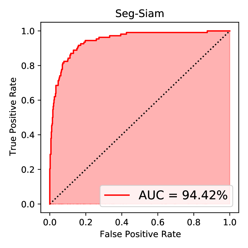
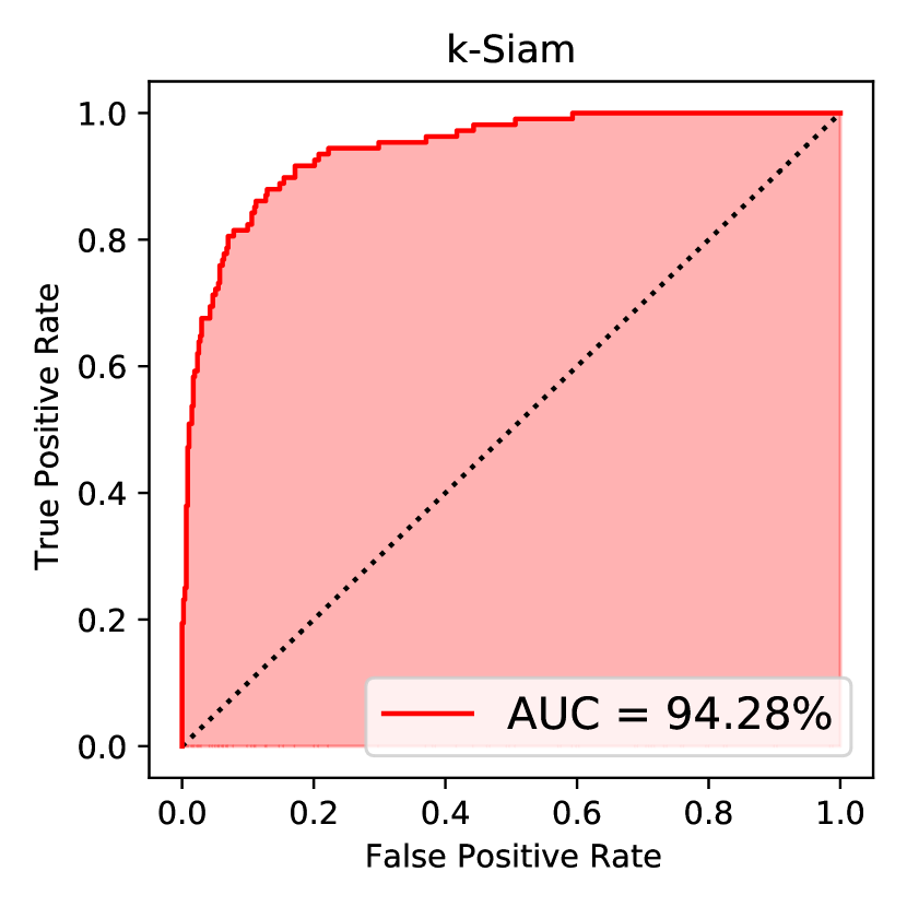
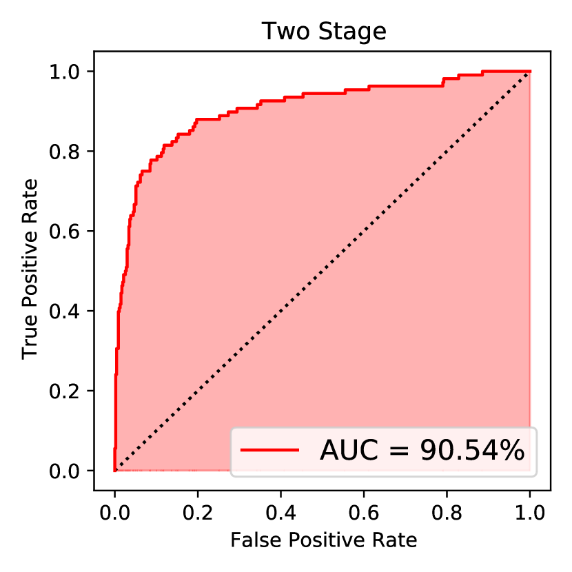
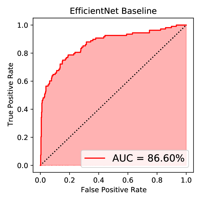
Figure 4: RoC curves of the four models on the MSI prediction task (n = 672).

3 Experiments and Results

3.1 MSI Prediction

We performed an ablation study on the CancerScout colon data to evaluate the quality and features of our model. In total, we compare the performance of four pipelines in the MSI prediction task. The first, $k$-Siam, uses random tile selection followed by the $k$-Siamese network described in Section 1. Seg-Siam uses tumor segmentation for tile selection followed by a $k$-Siamese network. Two Stage uses tumor segmentation for tile selection followed by tile-wise classification, implementing the standard two-stage approach. The EfficientNet baseline uses random tile selection and tile-wise classification. RoC curves together with the respective AUC values for all four pipelines are shown in Figure 4. In Table 2 we report the results of our pipelines compared to the methods discussed in [13].

3.1.1 Experimental Setup

For the tumor segmentation, we use use a PAN [15] based model with Efficientnet [30] backbone. This approach yields a validation Intersection over Union (IoU) performance of $98\text{\,}\mathrm{\char 37\relax}$. We use Efficientnet-B0 as base-classifier for all our experiments. Prediction aggregation is performed by averaging the confidences of all processed tiles. We use the same training and data-augmentation pipeline for all four models. For a fair comparison, we perform a random hyperparameter search with a total of $96$ runs per model over the most influential training parameters. The parameters considered, their range and optimal values are given in Table 2.

We evaluate the performance of our models using a $5$ fold patient-level cross-validation. We use fold $0$ for the hyperparameter search and folds $1$ to $4$ as test-set for evaluation. No parameter-tuning, threshold selection or training decisions are done using those test folds. In particular, we did not do any early stopping based on the evaluation score, but rather train the model to the end and evaluate model performance after the final epoch.

Gene	Preva-lance	Ours	Ref.[11]
		[AUC]	[AUC]
PIK3CA	$35\text{\,}\mathrm{\char 37\relax}$	0.64	$0.63$
TP53	$33\text{\,}\mathrm{\char 37\relax}$	0.80	$0.78$
CDH1	$13\text{\,}\mathrm{\char 37\relax}$	0.82	—
GATA3	$12\text{\,}\mathrm{\char 37\relax}$	0.64	<$0.62$
KMT2C	$10\text{\,}\mathrm{\char 37\relax}$	$0.53$	<$0.62$
MAP3K1	$8\text{\,}\mathrm{\char 37\relax}$	$0.47$	$0.62$
PTEN	$6\text{\,}\mathrm{\char 37\relax}$	0.75	<$0.62$
NCOR1	$5\text{\,}\mathrm{\char 37\relax}$	$0.51$	—

(a) Breast (n = 761)

Gene	Preva-lance	Ours	Ref.[11]
		[AUC]	[AUC]
APC	$74\text{\,}\mathrm{\char 37\relax}$	0.66	$0.65$
TP53	$60\text{\,}\mathrm{\char 37\relax}$	0.74	$0.68$
KRAS	$42\text{\,}\mathrm{\char 37\relax}$	$0.63$	<$0.65$
PIK3CA	$32\text{\,}\mathrm{\char 37\relax}$	$0.54$	<$0.65$
FAT4	$27\text{\,}\mathrm{\char 37\relax}$	$0.68$	—
KMT2D	$17\text{\,}\mathrm{\char 37\relax}$	$0.74$	0.76
BRAF	$17\text{\,}\mathrm{\char 37\relax}$	0.75	$0.67$
FBXW7	$16\text{\,}\mathrm{\char 37\relax}$	$0.63$	<$0.65$

(b) Colon (n = 268)

Gene	Preva-lance	Ours	Ref.[11]
		[AUC]	[AUC]
TP53	$50\text{\,}\mathrm{\char 37\relax}$	$0.71$	0.72
KRAS	$29\text{\,}\mathrm{\char 37\relax}$	0.62	<$0.6$
FAT4	$15\text{\,}\mathrm{\char 37\relax}$	$0.67$	—
STK11	$14\text{\,}\mathrm{\char 37\relax}$	0.65	$0.6$
EGFR	$13\text{\,}\mathrm{\char 37\relax}$	0.70	<$0.6$
KMT2C	$13\text{\,}\mathrm{\char 37\relax}$	$0.49$	<$0.6$
NF1	$12\text{\,}\mathrm{\char 37\relax}$	$0.57$	<$0.6$
SETBP1	$10\text{\,}\mathrm{\char 37\relax}$	$0.59$	<$0.6$

(c) Lung (n = 461)

Table 3: RoC AUC scores for genetic mutation prediction on TCGA Data.

3.2 Detecting Molecular Alterations

To gain further insights into the performance of our approach, we address the task of detecting molecular alterations from image features using the datasets discussed in Section 2.2 and compare our results to the study by Kather et al. [11]. For our study, we consider the top $8$ most prevalently mutated genes in each cohort and report the AUC scores in Table 3. Note that this differs from the approach used in [11], who evaluate the prediction performance on a total of $95$ known cancer driving genes and report the top $8$ highest scoring results.

3.2.1 Experimental Setup

We employ a patient-level $5$-fold cross-validation and use all folds as test-set. No parameter-tuning, thresholds or training decisions are done using those folds. We use the default parameters of our model discussed in Section 1.0.2 and train the model with these parameters only once on each of the $5$ folds. In addition, we do not apply any early stopping based on test scores, but train the model for $72$ epochs and evaluate the scores after the final epoch. We use a multi-label classification approach for this experiment. We train one network per dataset, each with $8$ binary classification outputs. We apply a softmax-crossentropy loss on each of them and average them (without weights) for training. Note that this approach is different from [11] who train a separate network for each gene.

The datasets contain multiple slides for some patients. For training, we choose one slide during each epoch for each patient at random. For inference, we average the confidences over all slides per patient. We perform a patient-level split, i.e. all slides of a patient are part of the same fold.

We compare our results to Kather et al. [11], since the study also performs patient-level cross-validation on their entire cohort. We note, that our cohort is slightly different from the cohort used in the reference study [11] for a number of reasons. Note that Kather et al. manually inspect all slides in the cohort and remove slides of subpar quality. In addition, a number of diagnostic slides have been removed from the TCGA dataset in $2021$, due to PII leaking in the images. Lastly, [11] uses a custom bioinformatics pipeline to compute the mutation information from the raw NGS data which yields target data for more patients. In summary, the reference study [11] uses a larger, higher quality dataset.

4 Discussion & Conclusion

This paper presents a novel $k$-Siamese convolutional neural network architecture for the classification of whole slide images in digital pathology. The method is trained end-to-end and does not require auxiliary annotations, which are tedious, time-consuming, and expensive to generate.

In our ablation study, we show that our method is able to clearly outperform commonly used two-stage approaches. We observe that adding a segmentation step to our model only leads to very minor improvement in the AUC score, which proofs that the $k$-Siamese model provides an efficient way of dealing with the label noise issue inherent to tile based processing. In addition, our experiments confirm the results shown in [13] that many recently proposed end-to-end methods are unable to outperform the widely used two-stage prediction pipeline. Those methods effectively trade annotation effort for prediction performance. In contrast, our approach is able to deliver state-of-the-art performance without requiring auxiliary annotations.

Further experiments on TCGA data reveal that our approach is also highly competitive with the published results by Kather et al. [11]: for most genes, our method is able to produce a higher response, painting a clearer picture which mutations have an impact on the morphology of the tumor. In contrast to [11], we are able to produce these results based exclusively on publicly available data, without the need for additional histological annotations. This makes it much easier to reproduce our results, but also allows to explore many more questions and tasks with minimal efforts.

We hope that the straight-forward implementation of our method, combined with its ability to outperform state-of-the-art approaches, will support further research on the identification of cancer phenotypes by digital pathology and ultimately enable personalized therapies for more patients in future.

4.0.1 Acknowledgements

The research presented in this work was funded by the German Federal Ministry of Education and Research (BMBF) as part of the CancerScout project (13GW0451). We thank all members of the CancerScout Consortium for their contributions, in particular Rico Brendtke and Tessa Rosenthal for organizational and administrative support as well as Sven Winkelmann and Monica Toma for performing various tasks in relation to data privacy, storage and transfer. In addition, we like to thank Christian Marzahl for his support during the installation and adaptation of the EXACT label server. Last but not least, we like to thank Matthias Siebert and Tobias Heckel for insightful discussions about the TCGA Dataset and the associated Omics data.

References

- [1] Campanella, G., Hanna, M.G., Geneslaw, L., Miraflor, A., Werneck Krauss Silva, V., Busam, K.J., Brogi, E., Reuter, V.E., Klimstra, D.S., Fuchs, T.J.: Clinical-grade computational pathology using weakly supervised deep learning on whole slide images. Nature medicine 25(8), 1301–1309 (2019)
- [2] Chen, H., Han, X., Fan, X., Lou, X., Liu, H., Huang, J., Yao, J.: Rectified cross-entropy and upper transition loss for weakly supervised whole slide image classifier. In: International Conference on Medical Image Computing and Computer-Assisted Intervention. pp. 351–359. Springer (2019)
- [3] Coudray, N., Ocampo, P.S., Sakellaropoulos, T., Narula, N., Snuderl, M., Fenyö, D., Moreira, A.L., Razavian, N., Tsirigos, A.: Classification and mutation prediction from non–small cell lung cancer histopathology images using deep learning. Nature medicine 24(10), 1559–1567 (2018)
- [4] Echle, A., Grabsch, H.I., Quirke, P., van den Brandt, P.A., West, N.P., Hutchins, G.G., Heij, L.R., Tan, X., Richman, S.D., Krause, J., et al.: Clinical-grade detection of microsatellite instability in colorectal tumors by deep learning. Gastroenterology 159(4), 1406–1416 (2020)
- [5] Echle, A., Rindtorff, N.T., Brinker, T.J., Luedde, T., Pearson, A.T., Kather, J.N.: Deep learning in cancer pathology: a new generation of clinical biomarkers. British journal of cancer 124(4), 686–696 (2021)
- [6] Ellrott, K., Bailey, M.H., Saksena, G., Covington, K.R., Kandoth, C., Stewart, C., Hess, J., Ma, S., Chiotti, K.E., McLellan, M., et al.: Scalable open science approach for mutation calling of tumor exomes using multiple genomic pipelines. Cell systems 6(3), 271–281 (2018)
- [7] Fu, Y., Jung, A.W., Torne, R.V., Gonzalez, S., Vöhringer, H., Shmatko, A., Yates, L.R., Jimenez-Linan, M., Moore, L., Gerstung, M.: Pan-cancer computational histopathology reveals mutations, tumor composition and prognosis. Nature Cancer 1(8), 800–810 (2020)
- [8] Goyal, P., Dollár, P., Girshick, R., Noordhuis, P., Wesolowski, L., Kyrola, A., Tulloch, A., Jia, Y., He, K.: Accurate, large minibatch sgd: Training imagenet in 1 hour. arXiv preprint arXiv:1706.02677 (2017)
- [9] Hou, L., Samaras, D., Kurc, T.M., Gao, Y., Davis, J.E., Saltz, J.H.: Patch-based convolutional neural network for whole slide tissue image classification. In: Proceedings of the IEEE conference on computer vision and pattern recognition. pp. 2424–2433 (2016)
- [10] Huang, G., Sun, Y., Liu, Z., Sedra, D., Weinberger, K.Q.: Deep networks with stochastic depth. In: European conference on computer vision. pp. 646–661. Springer (2016)
- [11] Kather, J.N., Heij, L.R., Grabsch, H.I., Loeffler, C., Echle, A., Muti, H.S., Krause, J., Niehues, J.M., Sommer, K.A., Bankhead, P., et al.: Pan-cancer image-based detection of clinically actionable genetic alterations. Nature Cancer 1(8), 789–799 (2020)
- [12] Kingma, D.P., Ba, J.: Adam: A method for stochastic optimization. arXiv preprint arXiv:1412.6980 (2014)
- [13] Laleh, N.G., Muti, H.S., Loeffler, C.M.L., Echle, A., Saldanha, O.L., Mahmood, F., Lu, M.Y., Trautwein, C., Langer, R., Dislich, B., et al.: Benchmarking artificial intelligence methods for end-to-end computational pathology. bioRxiv (2021)
- [14] Lee, H., Seo, J., Lee, G., Park, J., Yeo, D., Hong, A.: Two-stage classification method for msi status prediction based on deep learning approach. Applied Sciences 11(1), 254 (2021)
- [15] Li, H., Xiong, P., An, J., Wang, L.: Pyramid attention network for semantic segmentation
- [16] Liu, W., Rabinovich, A., Berg, A.C.: Parsenet: Looking wider to see better. arXiv preprint arXiv:1506.04579 (2015)
- [17] Lu, M.Y., Williamson, D.F., Chen, T.Y., Chen, R.J., Barbieri, M., Mahmood, F.: Data-efficient and weakly supervised computational pathology on whole-slide images. Nature biomedical engineering 5(6), 555–570 (2021)
- [18] Marzahl, C., Aubreville, M., Bertram, C.A., Maier, J., Bergler, C., Kröger, C., Voigt, J., Breininger, K., Klopfleisch, R., Maier, A.: Exact: a collaboration toolset for algorithm-aided annotation of images with annotation version control. Scientific reports 11(1), 1–11 (2021)
- [19] Micikevicius, P., Narang, S., Alben, J., Diamos, G., Elsen, E., Garcia, D., Ginsburg, B., Houston, M., Kuchaiev, O., Venkatesh, G., et al.: Mixed precision training. arXiv preprint arXiv:1710.03740 (2017)
- [20] Nagpal, K., Foote, D., Liu, Y., Chen, P.H.C., Wulczyn, E., Tan, F., Olson, N., Smith, J.L., Mohtashamian, A., Wren, J.H., et al.: Development and validation of a deep learning algorithm for improving gleason scoring of prostate cancer. NPJ digital medicine 2(1), 1–10 (2019)
- [21] Nazeri, K., Aminpour, A., Ebrahimi, M.: Two-stage convolutional neural network for breast cancer histology image classification. In: International Conference Image Analysis and Recognition. pp. 717–726. Springer (2018)
- [22] Network, C.G.A., et al.: Comprehensive molecular characterization of human colon and rectal cancer. Nature 487(7407), 330 (2012)
- [23] Network, T.C.G.A., et al.: Comprehensive molecular portraits of human breast tumours. Nature 490(7418), 61–70 (2012)
- [24] Network, T.C.G.A., et al.: Comprehensive molecular profiling of lung adenocarcinoma: The cancer genome atlas research network. Nature 511(7511), 543–550 (2014)
- [25] Shao, Z., Bian, H., Chen, Y., Wang, Y., Zhang, J., Ji, X., et al.: Transmil: Transformer based correlated multiple instance learning for whole slide image classification. Advances in Neural Information Processing Systems 34 (2021)
- [26] Sharma, Y., Shrivastava, A., Ehsan, L., Moskaluk, C.A., Syed, S., Brown, D.: Cluster-to-conquer: A framework for end-to-end multi-instance learning for whole slide image classification. In: Medical Imaging with Deep Learning. pp. 682–698. PMLR (2021)
- [27] Sondka, Z., Bamford, S., Cole, C.G., Ward, S.A., Dunham, I., Forbes, S.A.: The cosmic cancer gene census: describing genetic dysfunction across all human cancers. Nature Reviews Cancer 18(11), 696–705 (2018)
- [28] Srivastava, N., Hinton, G., Krizhevsky, A., Sutskever, I., Salakhutdinov, R.: Dropout: a simple way to prevent neural networks from overfitting. The journal of machine learning research 15(1), 1929–1958 (2014)
- [29] Ström, P., Kartasalo, K., Olsson, H., Solorzano, L., Delahunt, B., Berney, D., Bostwick, D., Evans, A., Grignon, D., Humphrey, P., et al.: Pathologist-level grading of prostate biopsies with artificial intelligence. corr (2019) (1907)
- [30] Tan, M., Le, Q.: Efficientnet: Rethinking model scaling for convolutional neural networks. In: International conference on machine learning. pp. 6105–6114. PMLR (2019)
- [31] Zhang, C., Bengio, S., Hardt, M., Recht, B., Vinyals, O.: Understanding deep learning requires rethinking generalization (2016). arXiv preprint:1611.03530 (2017)