TTP22-042, P3H-22-066
Singlet and non-singlet three-loop massive form factors

Abstract

We consider Quantum Chromodynamics with external vector, axial-vector, scalar and pseudo-scalar currents and compute three-loop corrections to the corresponding vertex function taking into account massive quarks. We consider all non-singlet contributions as well as those singlet contributions where the external current couples to a massive quark loop. We apply a semi-numerical method which is based on expansions around singular and regular kinematical points. They are matched at intermediate values of the squared partonic center-of-mass energy $s$ which allows to cover the whole kinematic range for negative and positive values of $s$. Our method permits a systematic increase of the precision by varying the expansion depth and the choice of the intermediate matching points. In our current set-up we have at least seven significant digits for the finite contribution of all form factors. We present our results as a combination of series expansions and interpolation functions which allows for a straightforward use in practical applications.

1 Introduction

Form factors are important building blocks for a number of processes. For example, they constitute the virtual corrections for lepton pair production via the Drell-Yan process, for Higgs boson production in gluon fusion and for Higgs boson decay into heavy quarks. For many processes there are precise experimental results such that higher-order corrections have to be included in the theory predictions. This is particularly true for QCD corrections, the topic of this paper.

There is a rapid increase in complexity when increasing the number of loops for a given process and often one has to rely on approximations valid in certain regions of phase space, in case one wants to perform analytic calculations. Alternatively, it is possible to use numerical methods, which, however, are less flexible in practical applications of the results.

In this paper we consider three-loop corrections to massive form factors in QCD. We use a method which leads to compact expansions of the bare three-loop expressions around kinematical points with high-precision numerical coefficients. Their numerical evaluation is fast and their combination covers the whole kinematic range. The counterterms are known in analytic form and allow for a flexible construction of finite expressions in different renormalization schemes.

We define the external vector, axial-vector, scalar and pseudo-scalar currents via

$$j_{\mu}^{v} = \bar{\psi}\gamma_{\mu}\psi\,,$$

$$j_{\mu}^{a} = \bar{\psi}\gamma_{\mu}\gamma_{5}\psi\,,$$

$$j^{s} = m\,\bar{\psi}\psi\,,$$

$$j^{p} = \mathrm{i}m\,\bar{\psi}\gamma_{5}\psi\,.$$ (1)

The heavy quark mass $m$ has been introduced in the scalar and pseudo-scalar currents for convenience such that all currents have vanishing anomalous dimensions [2].

The three-point functions with an external quark-anti-quark pair, which result from the currents in Eq. (1), can be decomposed into six form factors given by

$$\Gamma_{\mu}^{v}(q_{1},q_{2}) = F_{1}^{v}(q^{2})\gamma_{\mu}-\frac{\mathrm{i}}{2m}F_{2}^{v}(q^{2})\sigma_{\mu\nu}q^{\nu}\,,$$

$$\Gamma_{\mu}^{a}(q_{1},q_{2}) = F_{1}^{a}(q^{2})\gamma_{\mu}\gamma_{5}{-\frac{1}{2m}F_{2}^{a}(q^{2})q_{\mu}}\gamma_{5}\,,$$

$$\Gamma^{s}(q_{1},q_{2}) = {m}F^{s}(q^{2})\,,$$

$$\Gamma^{p}(q_{1},q_{2}) = {\mathrm{i}m}F^{p}(q^{2}){\gamma_{5}}\,.$$ (2)

Here the momentum $q_{1}$ ($q_{2}$) is incoming (outgoing) and $q=q_{1}-q_{2}$ is the outgoing momentum at the current $j^{\delta}$ with $q^{2}=s$. The external quarks are on-shell, i.e. $q_{1}^{2}=q_{2}^{2}=m^{2}$, and we have $\sigma^{\mu\nu}=\mathrm{i}[\gamma^{\mu},\gamma^{\nu}]/2$. We note that in all cases the colour structure is a simple Kronecker delta in the fundamental colour indices of the external quarks and not written out explicitly.

We distinguish singlet and non-singlet form factors. In the first case the external current couples to a closed quark loop which is connected to the quark line in the final state via gluons. In the non-singlet case the external current couples directly to the final-state quarks. In this paper we consider the complete non-singlet contributions as well as those singlet contributions where the closed quark loop has the same mass as the external quarks. While we consider all four currents in the non-singlet case, we only consider the vector, scalar and pseudo-scalar currents in the singlet case. The proper treatment of the axial-vector contribution requires the singlet contributions with a massless closed quark loop, which is postponed to the future.

We define the perturbative expansion of the scalar form factors as

$$F=\sum_{n\geq 0}F^{(n)}\left(\frac{\alpha_{s}(\mu)}{\pi}\right)^{n}\,,$$ (3)

where at lowest order we have $F_{1}^{v,(0)}=F_{1}^{a,(0)}=F^{s,(0)}=F^{p,(0)}=1$ and $F_{2}^{v,(0)}=F_{2}^{a,(0)}=0$. The three-loop non-singlet form factors can be decomposed into the ten colour factors

$$\{C_{F}^{3},C_{F}C_{A}^{2},C_{F}^{2}C_{A},C_{F}^{2}T_{F}n_{l},C_{F}C_{A}T_{F}n_{l},C_{F}T_{F}^{2}n_{l}^{2},C_{F}T_{F}^{2}n_{l}n_{h},C_{F}^{2}T_{F}n_{h},$$

$$C_{F}C_{A}T_{F}n_{h},C_{F}T_{F}^{2}n_{h}^{2}\}\,,$$ (4)

where $C_{F}=T_{F}(N_{C}^{2}-1)/N_{C}$ and $C_{A}=2T_{F}N_{C}$ are the quadratic Casimir operators of the $\mathrm{SU}(N_{C})$ gauge group in the fundamental and adjoint representation, respectively, $n_{l}$ is the number of massless quark flavors, and $T_{F}=1/2$. For convenience we introduce $n_{h}=1$ for closed quark loops which have the same mass as the external quarks.

The singlet form factors start at two-loop order. Due to Furry’s theorem the vector form factor is non-zero only at three-loop order, but there are non-zero results for $F^{s,(2)}_{\rm sing}$ and $F^{p,(2)}_{\rm sing}$. For the three-loop singlet form factors we have the colour factors

$$\{C_{F}^{2}T_{F}n_{h},C_{F}C_{A}T_{F}n_{h},C_{F}T_{F}^{2}n_{h}^{2},C_{F}T_{F}^{2}n_{l}n_{h},n_{h}(d^{abc})^{2}/N_{C}\}\,,$$ (5)

where $(d^{abc})^{2}=(N_{C}^{2}-1)(N_{C}^{2}-4)/(16N_{C})$ arises from Feynman diagrams in which the closed fermion loop is connected to the external quarks by three gluons, see Fig. 1(d). This is the only colour structure present in $F_{1,\rm sing}^{v,(3)}$ and $F_{2,\rm sing}^{v,(3)}$. On the other hand, the scalar and pseudo-scalar form factors do not have this colour structure.

Two-loop corrections to the vector form factors have been computed about 20 years ago, first in the context of QED [3, 4] and later also for QCD [5] (see also Ref. [6] for the fermionic contributions). Several groups have provided cross checks and computed higher order terms in $\epsilon$ [7, 8, 9, 10, 11]. Higher order perturbative contributions in the high-energy limit of the form factors have been predicted in Refs. [12, 7, 9] using renormalization group equations. Two-loop axial-vector, scalar and pseudo-scalar contributions have been computed in Refs. [13, 14, 15, 10].

Analytic three-loop corrections to the form factors have first been considered in the large-$N_{C}$ limit [8, 16, 17, 18] where only planar integrals have to be computed. The first non-planar contributions appear in the light-fermion contributions which are available from Ref. [11]. In Ref. [19] all contributions with a closed heavy quark loop have been considered and around 2000 expansion terms around $s=0$ have been computed. Let us also mention that all-order corrections to massive form factors in the large-$\beta_{0}$ limit have been considered in Ref. [20], where $\beta_{0}$ is the one-loop correction to the QCD beta function.

In Ref. [21] we computed first complete results for the vector form factors $F_{1}^{v}$ and $F_{2}^{v}$ taking into account all colour factors and covering the whole $s$ range. In this work we present details of the computational method and extend the results to the axial-vector, scalar and pseudo-scalar currents. We present results for the non-singlet contributions, where the external current couples to the quarks in the final state. In this case it is possible to use anti-commuting $\gamma_{5}$. Furthermore, we consider the singlet contributions, where the external current couples to a closed massive quark loop. For the treatment of $\gamma_{5}$ in the pseudo-scalar singlet case we follow Ref. [22]. Sample Feynman diagrams for the heavy-quark form factors are shown in Fig. 1.

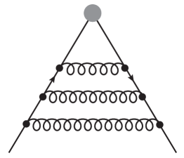
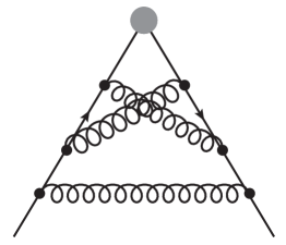
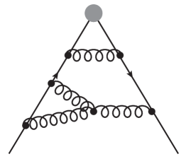
(a)	(b)	(c)
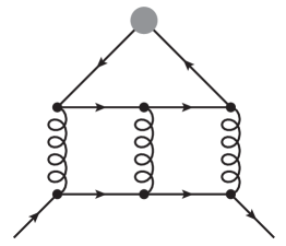
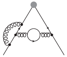
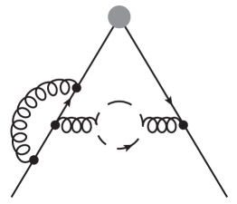
(d)	(e)	(f)

Figure 1: Sample diagrams contributing to the form factors. Solid, dashed and curly lines represent massive quarks, massless quarks and gluons, respectively. The blob refers to one of the external currents given in Eq. (1). Diagram (d) is a representative for the singlet contribution. Here the quark in the closed loop is massive.

Form factors with massless external quarks are available to higher order in perturbation theory. They have been computed to three-loop order in Refs. [23, 24, 25, 26, 27, 28]. Recently even four-loop corrections became available [29, 30, 31, 32, 33, 34, 35, 36, 37, 38]. In Ref. [39] three-loop singlet corrections to massless axial-vector form factors have been considered where the external current couples to a massive closed quark loop.

The remainder of this paper is organized as follows: In Section 2 we describe the setup used for the computation of the amplitudes for the form factors. In Section 3 we describe our approach for the construction of the approximations of the master integrals. Section 4 is dedicated to the singlet form factors and the renormalization and infrared subtraction is discussed in Section 5. Our results are presented in Section 6. We conclude in Section 7. Supplementary material is relegated to the Appendix. In Appendix A we provide results for the three-loop on-shell integrals with special emphasis on the higher order terms in the $\epsilon$ expansion, which we needed as boundary conditions to determine the master integrals. Appendix B contains the collection of the plots which show the accuracy of the pole cancellation and in Appendix C we present semi-analytic expansions around $s=0,4m^{2}$ and $\infty$.

2 Reduction to master integrals and choice of basis

In this Section we provide details for the non-singlet form factors; the discussion for the singlet form factors is postponed to Section 4.

We generate the amplitudes with qgraf [40] and use q2e and exp [41, 42, 43] to rewrite the output to FORM [44] notation and map each diagram to a predefined integral family. In this way we can express the form factors as linear combinations of scalar Feynman integrals with twelve indices where nine correspond to the exponents of propagators and the remaining three to the exponents of irreducible numerators. In total we have $34$ different integral families.

Before performing the reduction of the Feynman integrals contributing to the form factors, we improve the basis by getting rid of those denominators in the coefficients of the master integrals which are multivariate polynomials. Since the ratio $s/m^{2}$ is the only kinematic variable, it is possible to find a basis such that the denominators completely factorize into univariate polynomials of either $s/m^{2}$ or $d$ [45, 46]. Moreover, it turns out that we can choose a basis such that all polynomials of $s/m^{2}$ in the denominators are linear polynomials raised to some power. We call this basis good in the following. To construct this basis we first reduce all integrals up to the top-level sector and with up to two dots for every integral family individually with the help of Kira [47, 48] employing Fermat [49]. As initial basis we simply take the default master integrals found with the integral ordering $6$ of Kira, i.e. the sectors are primarily ordered by the number of lines and dots are preferred over scalar products. These reduction tables then serve as input to search for a good basis for every family with the help of an improved version of ImproveMaster.m developed in Ref. [45]. The construction of a good basis takes about three hours for the most expensive families and almost all of that runtime is spent for the reduction.

The actual reduction of the integrals for the form factors is also performed with Kira employing Fermat. First, we reduce the integrals for every family individually to the good basis of this family. The most expensive families run for about a week on eight cores and require about $200$ GiB of memory. The resulting reduction tables, especially the denominators, are simplified by using Mathematica to factorize the expressions which is not done by Kira and Fermat. Secondly, we employ symmetries between the families to reduce the number of master integrals. To this end we sort the families by ascending number of master integrals and use Kira to reduce the good master integrals for every family to those of easier families if possible. This reduces the number of master integrals from $3131$ to $422$. $136$ of these master integrals are needed for the fermionic contributions with at least one closed massive or massless quark loop. This step takes about one day and can be done in parallel to the individual reductions of all families since the non-minimal good basis is already known.

We set up the differential equations for the master integrals by differentiating the master integrals with respect to $s/m^{2}$ with the help of LiteRed [50, 51] and reducing the resulting integrals again to master integrals with Kira. Also this step is performed on a per-family basis and the already known symmetry tables are only inserted in the very last step. The construction of the differential equations takes at most a few hours per family. The only complication at this point is that a few blocks on the diagonal of the system of differential equations contain unfavorable pole structures that prohibit a solution of the master integrals as series in $\epsilon$. However, this problem can be solved by searching the available reduction tables for integrals in the affected sectors with a pole in front of one of the master integrals of the same sector. Inverting the relation, i.e. switching integral and master integral, thus introduces a positive power of $\epsilon$ and improves on the pole structure [52]. By repeating this step all sectors can be made solvable. For our problem this can be achieved without spoiling the good properties of the basis. Let us emphasize that we explicitly did not try to get rid of all poles in our reduction tables because this would most certainly spoil the good properties.

3 Method

In order to (numerically) solve the master integrals we apply the method of analytical expansions and numerical matching introduced in Ref. [53]. Let us briefly summarize the basic idea:

• After establishing a system of differential equations for the master integrals, we calculate initial values at a kinematic point where the integrals simplify.

• We construct an analytic series expansion around this kinematic point by inserting a suitable ansatz into the system of differential equations, re-expanding in $\epsilon$ and around the special kinematic point, establishing a system of linear equations for the expansion coefficients and solving it in terms of a small set of boundary coefficients. We use the information from step (a) to fix these coefficients analytically.

• Construct an analytic expansion around a neighboring kinematic point. Here we cannot fix the boundary constants analytically, but we can evaluate both expansions at a kinematic point where the radii of convergence of both expansions overlap and use these values as numerical initial conditions.

• Repeat this procedure until the whole kinematic interval of interest is mapped out with partially overlapping series expansions.

In the following we give details on how we applied this method to the calculation of the massive form factors. We concentrate on the non-singlet form factors; details for the singlet form factors are provided in Section 4.

(a) Calculation of initial values

For our initial expansion we choose the value $s=0$. At this point the master integrals simplify to on-shell propagator integrals which are well studied in the literature [54, 55, 25]. However, one obstacle in obtaining the initial values for our system of differential equations is the appearance of high spurious poles in the dimensional regulator $\epsilon$ in the physical amplitude and the differential equation. This requires the knowledge of some master integrals beyond the order given in Ref. [25]. The same problem was also encountered in Ref. [19], where a subset of integrals was already obtained to sufficiently high order in $\epsilon$. We extended the calculation of the remaining integrals to the order in $\epsilon$ needed in our approach. Details on the calculation and the results are given in Appendix A. We note that due to the spurious poles of $\mathcal{O}(1/\epsilon^{8})$ we need some integrals up to transcendental weight 9, however, in the physical amplitude all contributions with weight higher than 5 cancel.

(b) Construction of series expansions

In order to construct series expansions around specific values of $s$ we insert a suitable ansatz into the differential equation, re-expand in $\epsilon$ and around the chosen value of $s$ and construct a system of linear equations for the expansion coefficients of the ansatz by equating coefficients. The suitable ansatz can be found from physical considerations. We only have three kinematic points with non-analytical expansions. They correspond to the two-particle threshold $s=4m^{2}$, the four-particle threshold $s=16m^{2}$ and the high-energy expansion $s\to\pm\infty$. For these three expansion points we have to use a power-log ansatz. Since the threshold expansions are governed by the particle velocities, we use the variables $z=\sqrt{4-s}$ and $z=\sqrt{16-s}$ for the two- and four-particle thresholds respectively. The ansatz for a master integral $I_{n}$ is then given by

$$I_{n} = \sum\limits_{i=-o}^{\infty}\sum\limits_{j=-k}^{\infty}\sum\limits_{m=0}^{i+o}c_{n,i,j,m}\epsilon^{i}z^{l}\ln^{m}(z)~{}.$$ (6)

For the present three-loop problem we have $o=3$ and we choose $k=10$ as a conservative lower bound. In principle both lower values depend on the master integral and can be determined beforehand. In practice, we choose them uniformly for all master integrals for simplicity. The high-energy expansion can be performed in the variable $z=1/(-s)$, but one has to allow for Sudakov-like double logarithms in the ansatz. The upper summation variable of the sum over $m$ in Eq. (6) has therefore to be modified to $i+2o$. All other expansions are given by simple Taylor expansions in the variable $z=s_{0}-s$, with $s_{0}$ the value we want to expand around. Thus, the sum over $m$ can be dropped and $k=0$.

The resulting system of linear equations, which does not contain any variable anymore, is solved by Kira together with Fermat or FireFly [56, 57]. For the use with FireFly we use a special version of Kira which allows the efficient use of finite field methods and rational reconstruction even for systems without variables. We make sure to prefer boundary constants corresponding to low powers of $z$ and $\epsilon$ in the ansatz when solving the system.

(c) Numerical matching of neighboring expansions

Once we found the symbolic expansion around $s=0$ we can use the previously calculated initial values to fix the remaining boundary constants. This results in an analytic expansion of the master integrals around $s=0$, where we calculated 76 terms in the expansion. In a next step we construct a symbolic expansion around $s=1$. For $s=1$ the boundary constants cannot be easily fixed analytically. However, since the radii of convergence for the expansion around $s=0$ and $s=1$ overlap, we can use the numerical evaluation of the expansion around $s=0$ at $s=1/2$ to obtain numerical boundary conditions for the expansion around $s=1$.

In practice, we equate the expansions around $s=0$ and $s=1$ after setting $s=1/2$ to obtain a linear system of equations for the remaining boundary constants in the $s=1$ expansion. For analytical values at $s=1/2$ this system has a unique solution. However, due to the finite numerical precision this is not the case anymore and we have to be careful in solving the system. We proceed in the following way:

• In order to get numerically more stable results we rationalize the numbers in the system with a preset accuracy.

• We sort the equations with ascending number of appearing boundary constants and start by solving the equations one by one and insert the solutions back into the remaining equations. After inserting we rationalize again to the preset accuracy in order to avoid bigger and bigger rational numbers. Furthermore, we set numbers with absolute values smaller than a threshold to zero. This is important, since sometimes boundary conditions in the system are multiplied by very small numbers of the order of the preset accuracy. If we accidentally solve for these constants we introduce large values into the system of equations which render the solution of the system unstable.

• Sometimes after reinserting relations, which have been found before, back into the system, equations with no boundary constant remain. In an analytic matching these numbers would be identically zero. We use the absolute value of these remaining numbers to judge the accuracy of the matching.

To evaluate the stability of the final solution we solve the systems twice: once with rationalized coefficients with an accuracy of 500 digits and setting all numbers smaller than $10^{-100}$ to zero and once with rationalized coefficients with an accuracy of 100 digits and setting all numbers smaller than $10^{-50}$ to zero. We find agreement of both runs with the expected accuracy of $\sim 100$ digits.

(d) Mapping out the kinematics

In previous calculations of the form factors the variable $x$ defined by

$$s=-\frac{(1-x)^{2}}{x}$$ (7)

has been used. This choice of variable maps the special points of the physical amplitude corresponding to low energy ($s=0$), production threshold of two heavy quarks ($s=4m^{2}$) and the high-energy limit ($s=\pm\infty$) to the points $x=1,0,-1$ and, up to two-loop order, allows to express the final result in terms of harmonic polylogarithms. However, in our approach it turns out that the variable $x$ is not a good choice. One problem we encounter is that the production threshold of four heavy quarks, which starts contributing at three-loop order, is mapped to $x=4\sqrt{3}-7\approx-0.072$. As a consequence the expansion around $x=0$ has a very small radius of convergence and large numerical coefficients appear in the expansions, making the numerical solution less stable. In addition, we also have to construct expansions around the value of the new threshold. In principle this can be achieved by defining the square root as a symbol before passing the system of equations to Kira. However, this complicates the solution of the system considerably. We therefore choose to do the expansions in the variable $s$.

To obtain the results for the non-singlet form factors over the whole real axis we construct expansions at the values of

$$\frac{s_{0}}{m^{2}} = \Biggl{\{}-\infty,-32,-28,-24,-16,-12,-8,-4,0,1,2,5/2,3,7/2,$$ (8)

$$4,9/2,5,6,7,8,10,12,14,15,16,17,19,22,28,40,52\Biggr{\}}$$

starting from our initial expansion at $s=0$. The numerical matching between two neighboring expansions is always done close to the center of the interval. Some of these values are chosen to correspond to additional, unphysical poles in the differential equation which we observe at

$$\frac{s}{m^{2}}=\Biggl{\{}-4,-2,-1,-1/2,1/2,1,2,3,16/3\Biggr{\}}~{}.$$ (9)

However, it turns out that these additional poles are all spurious and do not spoil the convergence of the series expansions. Thus, expansions around $s/m^{2}=4,16,\infty$ are in principle sufficient to construct the form factors at arbitrary values of $s$. However, we find that this approach suffers from a slow convergence of the individual series expansions close to the singular points, which means that very deep expansions are required to get decent accuracy at the matching points. Since very deep expansions are expensive in our approach we trade the expansion depth with more expansions at intermediate points with a default expansion depth of $51$ terms. These intermediate points are all Taylor expansions and therefore quite inexpensive to calculate.

For series expansions close to a singular point we employ Möbius transformations, which have already been discussed in Ref. [58]. Assume, we want to expand around the point $x_{k}$ and there are singular points of the differential equations at $x_{k-1}$ and $x_{k+1}$ with $x_{k-1}<x_{k}<x_{k+1}$. Naively the radius of convergence is limited by the distance to the closer singular point. However, the variable transformation

$$y_{k}=\frac{(x-x_{k})(x_{k+1}-x_{k-1})}{(x-x_{k+1})(x_{k-1}-x_{k})+(x-x_{k-1})(x_{k+1}-x_{k})}$$ (10)

maps the points $x_{k-1}$, $x_{k}$, $x_{k+1}$ to $-1$, 0, 1. The radius of convergence of the series expansion is therefore extended into the direction of the farther singularity although the convergence at the boundaries can be quite slow. For example we construct the expansion around $s/m^{2}=7/2$ in the difference $x=7/2m^{2}-s$, but afterwards reexpress the result in

$$y = \frac{7m^{2}-2s}{2s-9m^{2}}~{}.$$ (11)

While the expansion in the variable $x$ converges for $s\in(3,4)$, the convergence for the expansion in $y$ is increased to $s\in(-\infty,4)$, making the evaluation at the matching point $s=15/4$ much more precise.

Let us comment on the resources needed to construct the series expansions in our approach. To set up the system of linear equations for the construction of the series expansions we use Mathematica and can trivially parallelize this step over all master integrals. For the most complicated master integrals this step takes around $1\,$h on a single core. The solution of the resulting system for a simple Taylor expansion over one prime field takes around $6\,$h and requires about $50\,$GiB of memory. In total around 50 evaluations are needed which can all run in parallel. The power-log expansions are more expensive to compute. Due to the Sudakov-like double logarithms the high-energy expansion is the most involved. Here the solution of the linear system of equations over one prime field takes around $10\,$d with a memory requirement of $250\,$GiB, but again the evaluation over 50 prime fields is enough to reconstruct the full result.

The idea to utilize the associated system of differential equations to obtain expansions or numerical evaluations of the master integrals has received a lot of attention especially in the recent past [59, 60, 61, 62, 58, 63, 64], and there are even public packages available which implement different algorithms [65, 66, 67, 68]. However, most of them have restrictions on the structure of the system of differential equations, e.g. it has to be triangular for SeaSyde [68] or Fuchsian without resonances for DESS [65], or on the solution, e.g. only formal power series [61]. Some methods also lack the proof that they can handle complicated physical problems with a few hundred master integrals. Here, we show that the method laid out above can be used to compute a nontrivial quantity, namely the massive form factors at three-loop order in QCD, and obtain precise numerical results over the whole parameter space.

4 Singlet contributions to the form factors

In this Section we discuss the calculation of the singlet contribution to the three-loop massive QCD form factors, i.e.  contributions of the type shown in Fig. 1(d) where the current couples to a closed heavy-quark loop. We present results for the vector, scalar and pseudo-scalar case. The axial-vector contribution is anomalous and needs the inclusion of singlet diagrams where the current couples to a closed light-quark loop. Since many of the technical details of the calculation closely follow the non-singlet case, we only discuss them briefly. We put special emphasis on the computation of the boundary conditions in the limit $s\to 0$ since the calculation is different from the one in the non-singlet case. Results for the singlet contribution are shown in Section 6 together with the non-singlet case.

To generate the amplitude in the singlet case we need 17 different integral families. The resulting list of scalar integrals is again reduced with Kira and Fermat where we find 316 master integrals after symmetrization over all families. In this case we not only make sure to reduce to a good basis, but in addition reduce the number of spurious poles in $\epsilon$. This is achieved with an improved version of ImproveMasters.m. Afterwards we again establish a closed system of differential equations with the help of LiteRed with subsequent reductions using Kira. Overall the reduction of the singlet diagrams is significantly simpler than the one in the non-singlet case.

In principle the whole method discussed in Sec. 3 can be directly applied to the singlet diagrams. However, the calculation of the boundary conditions at $s=0$ is more involved, since the singlet diagrams can possess massless cuts. Hence, a simple Taylor expansion around the limit $s=0$ is not sufficient, but we have to perform an asymptotic expansion. We realize the asymptotic expansion by the method of regions [69, 70], where the relevant regions can be found with the program asy.m [71].

Applying asy.m to the singlet master integrals we find that there are regions with three different scalings:

• region 1: $I\sim y^{-0\,\epsilon}$

• region 2: $I\sim y^{-2\,\epsilon}$

• region 3: $I\sim y^{-4\,\epsilon}$

with $y=\sqrt{-s/m^{2}}$. Region 1 corresponds to the hard region, where we can naively expand the integrands around $s=0$ and apply the same procedure as for the non-singlet diagrams to obtain the boundary conditions.

The expansions in the two soft regions 2 and 3 do not permit a straightforward diagrammatic expansion. In order to calculate the boundary conditions in these regions we perform the expansion on the level of the integral representation in terms of $\alpha$ parameters and use direct integration methods to solve the occurring integrals. Let us exemplify the calculation of the boundary conditions for the two soft regions for the most involved master integral $J$ we encounter. The corresponding graph is shown in Fig. 2.

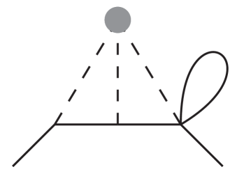
Figure 2: The graph corresponding to master integral $J$. Full (dashed) lines correspond to massive (massless) scalar propagators. The dot represents the influx of the external momentum $q$.

The Symanzik polynomials $\mathcal{U}$ and $\mathcal{F}$ for this diagram are given by

$$\mathcal{U} = \alpha_{5}\left(\left(\alpha_{3}+\alpha_{4}\right)\alpha_{6}+\alpha_{1}\left(\alpha_{3}+\alpha_{4}+\alpha_{6}\right)+\alpha_{2}\left(\alpha_{3}+\alpha_{4}+\alpha_{6}\right)\right)~{},$$ (12)

$$\mathcal{F} = \alpha_{2}\alpha_{4}\alpha_{5}\alpha_{6}{(-s)}+\alpha_{5}\biggl{(}\left(\alpha_{3}+\alpha_{4}+\alpha_{6}\right)\alpha_{1}^{2}+\left(\alpha_{3}^{2}+\left(\alpha_{5}+2\alpha_{6}\right)\alpha_{3}+\alpha_{5}\left(\alpha_{4}+\alpha_{6}\right)\right)\alpha_{1}$$ (13)

$$+\left(\alpha_{3}^{2}+\alpha_{5}\alpha_{3}+\alpha_{4}\alpha_{5}\right)\alpha_{6}+\alpha_{2}\left(\alpha_{3}^{2}+\alpha_{5}\alpha_{3}+\alpha_{5}\left(\alpha_{4}+\alpha_{6}\right)\right)\biggr{)}m^{2}~{},$$

and the master integral can be written as

$$J = \int\limits_{0}^{\infty}\left(\prod\limits_{i=1}^{6}{\rm d}\alpha_{i}\right)\ \mathcal{U}^{-d/2}e^{-\mathcal{F}/\mathcal{U}}.$$ (14)

With the help of asy.m we find the possible scalings of the $\alpha$-parameters to be $\{0,0,0,0,0,0\}$ or $\{-1,-2,-1,-2,0,-2\}$. The first scaling corresponds to the hard region, which we can calculate with the same method as in the non-singlet case. We obtain

$$J_{1} = e^{-3\gamma_{E}\epsilon}\Biggl{\{}\frac{\pi^{2}}{6\epsilon^{2}}+\frac{1}{\epsilon}\biggl{(}2\zeta_{3}+\frac{\pi^{2}}{2}\biggr{)}+6\zeta_{3}+\frac{79\pi^{4}}{360}+\frac{7\pi^{2}}{6}+\epsilon\biggl{(}\frac{5\pi^{2}\zeta_{3}}{3}+14\zeta_{3}+36\zeta_{5}$$ (15)

$$+\frac{79\pi^{4}}{120}+\frac{5\pi^{2}}{2}\biggr{)}+\epsilon^{2}\biggl{(}6\zeta_{3}^{2}+5\pi^{2}\zeta_{3}+30\zeta_{3}+108\zeta_{5}+\frac{17743\pi^{6}}{60480}+\frac{553\pi^{4}}{360}+\frac{31\pi^{2}}{6}\biggr{)}$$

$$+\mathcal{O}(\epsilon^{3})\Biggr{\}}~{}.$$

The second scaling corresponds to region 3, which can be seen by applying the scaling relations to the integrand in Eq. (14). In this region the $\mathcal{U}$ and $\mathcal{F}$ polynomials reduce to

$$\mathcal{F}_{3} = \alpha_{5}\left(\alpha_{4}\alpha_{6}+\alpha_{2}\left(\alpha_{4}+\alpha_{6}\right)\right)~{},$$ (16)

$$\mathcal{U}_{3} = \alpha_{5}\biggl{(}\alpha_{2}\alpha_{4}\alpha_{6}{(-s)}+\Bigl{(}\left(\alpha_{4}+\alpha_{6}\right)\alpha_{1}^{2}+2\alpha_{3}\alpha_{6}\alpha_{1}+\left(\alpha_{3}^{2}+\alpha_{4}\alpha_{5}\right)\alpha_{6}$$ (17)

$$+\alpha_{2}\left(\alpha_{3}^{2}+\alpha_{5}\left(\alpha_{4}+\alpha_{6}\right)\right)\Bigr{)}m^{2}\biggr{)}~{}.$$

To obtain our boundary condition in region 3 we therefore have to solve the integral

$$J_{3} = \int\limits_{0}^{\infty}\left(\prod\limits_{i=1}^{6}{\rm d}\alpha_{i}\right)\left(\mathcal{U}_{3}\right)^{2\epsilon-2}\exp\left(-\frac{\mathcal{F}_{3}}{\mathcal{U}_{3}}\right)~{}.$$ (18)

The $\alpha$ parameters $\alpha_{1}$, $\alpha_{2}$ and $\alpha_{5}$ can be integrated using the formulae

$$\int\limits_{0}^{\infty}{\rm d}\alpha\,\alpha^{a}\exp\left(-A\,\alpha\right) = \Gamma(1+a)A^{-1-a}~{},$$ (19)

$$\int\limits_{0}^{\infty}{\rm d}\alpha\,\alpha^{a}(1+\alpha)^{b} = \frac{\Gamma(1+a)\Gamma(-1-a-b)}{\Gamma(-b)}$$ (20)

together with suitable rescalings of the integration variables. In the end we are left with

$$J_{3} = y^{-4\epsilon}\frac{\Gamma(\epsilon-1){\Gamma(2\epsilon)}}{2}\int\limits_{0}^{\infty}{\rm d}\alpha_{3}\int\limits_{0}^{\infty}{\rm d}\alpha_{4}\int\limits_{0}^{\infty}{\rm d}\alpha_{6}\frac{\alpha_{4}^{-2\epsilon}\,\alpha_{6}^{-2\epsilon}\left(\alpha_{6}+\alpha_{4}(1+\alpha_{6})\right)^{3\epsilon-1}}{\alpha_{4}+\alpha_{6}+2\alpha_{3}\alpha_{6}+\alpha_{3}^{2}(1+\alpha_{6})}~{}.$$ (21)

The remaining integrals cannot be further reduced by applying the formulae in Eqs. (19) and (20). We find it convenient to integrate Eq. (21) with the help of the program HyperInt [72], since the divergent pieces for $\epsilon\to 0$ are already factored out into the $\Gamma$ functions and the integrand can be simply expanded in $\epsilon$. After performing the integrals the result is given by

$$J_{3} = y^{-4\epsilon}\pi^{2}e^{-3\gamma_{E}\epsilon}\Biggl{\{}-\frac{1}{6\epsilon^{2}}-\frac{7}{6\epsilon}+\frac{13\pi^{2}}{72}-\frac{43}{6}+\epsilon\left(\frac{59\zeta_{3}}{6}-\frac{259}{6}+\frac{91\pi^{2}}{72}\right)$$ (22)

$$+\epsilon^{2}\left(\frac{413\zeta_{3}}{6}-\frac{1555}{6}+\frac{559\pi^{2}}{72}+\frac{3767\pi^{4}}{8640}\right)+\mathcal{O}(\epsilon^{3})\Biggr{\}}~{}.$$

Region 2 does not contribute to the master integral $J$, so we have $J_{2}=0$. The complete boundary condition can be obtained by adding up the contributions of all regions:

$$J = J_{1}+J_{2}+J_{3}+\mathcal{O}(y)~{}.$$ (23)

Note that for regions 2 and 3 for all other boundary conditions the formulae in Eqs. (19) and (20) are sufficient to obtain the boundary in terms of $\Gamma$ functions and therefore exact in $\epsilon$.

After all boundary conditions for all three regions are found we again obtain analytic series expansions around $s=0$. In the singlet case we calculate symbolic expansions at the values of

$$\frac{s_{0}}{m^{2}} = \{-\infty,-32,-28,-24,-16,-12,-8,-4,-3,-2,-1,0,1,2,3,7/2,4,$$ (24)

$$9/2,5,6,7,8,10,12,14,15,16,17,19,22,28,40,52\}$$

and match numerically again starting from our initial expansion at $s=0$. The singular points at $s/m^{2}=4,16,\infty$ are shared among the singlet and non-singlet case. For the singlet diagrams also the point $s=0$ is a singular point and we need to perform a power-log expansion. Let us mention that in the singlet case the differential equation has the additional unphysical poles

$$\frac{s}{m^{2}} = \{-4,-2,-1/2,0,1,2,4,4\pm 8\mathrm{i},16/3,12,16\}\,.$$ (25)

5 Ultraviolet renormalization and infrared subtraction

The form factors develop both ultraviolet (UV) and infrared (IR) divergences. To account for the UV divergences we have to renormalize the quark mass, the strong coupling constant and the wave function of the external quarks. We denote the UV-renormalized form factors by $F^{\rm UVren}$ which still have poles in $\epsilon$ of IR nature. They are taken care of with the help of an IR renormalization factor in minimal subtraction, $Z$, which is constructed from the QCD beta function and the cusp anomalous dimension (see, e.g., Ref. [8]). It is convenient to consider $\log Z$ which is given by

$$\log Z = -\frac{\alpha_{s}(\mu)}{\pi}\frac{\Gamma_{\rm cusp}^{(1)}}{2\epsilon}+\left(\frac{\alpha_{s}(\mu)}{\pi}\right)^{2}\left(\frac{\beta_{0}\Gamma_{\rm cusp}^{(1)}}{16\epsilon^{2}}-\frac{\Gamma_{\rm cusp}^{(2)}}{4\epsilon}\right)$$ (26)

$$\mbox{}+\left(\frac{\alpha_{s}(\mu)}{\pi}\right)^{3}\left(-\frac{\beta_{0}^{2}\Gamma_{\rm cusp}^{(1)}}{96\epsilon^{3}}+\frac{\beta_{1}\Gamma_{\rm cusp}^{(1)}+4\beta_{0}\Gamma_{\rm cusp}^{(2)}}{96\epsilon^{2}}-\frac{\Gamma_{\rm cusp}^{(3)}}{6\epsilon}\right)\,,$$

with

$$\beta_{0} = \frac{11}{3}C_{A}-\frac{4}{3}T_{F}n_{l}\,,$$

$$\beta_{1} = \frac{34}{3}C_{A}^{2}-4C_{F}T_{F}n_{l}-\frac{20}{3}C_{A}T_{F}n_{l}\,.$$ (27)

$\Gamma_{\rm cusp}^{(i)}$ are the expansion coefficients of the cusp anomalous dimension defined through

$$\Gamma_{\rm cusp} = \sum_{i\geq 1}\Gamma_{\rm cusp}^{(i)}\left(\frac{{\alpha}_{s}}{\pi}\right)^{i}\,.$$ (28)

The cusp anomalous dimension in QCD is available to three loops from Refs. [73, 74, 75, 76].

Using $Z$, we can define a finite form factor via

$$F^{\rm UVren} = ZF^{f}\,.$$ (29)

Spelling out this equations leads to

$$F^{f} = Z^{-1}F^{\rm UVren}$$ (30)

$$= Z^{-1}\left(F^{(1+2+\rm CT)}+F^{(3)}\right)\,,$$

where $F^{(1+2+\rm CT)}$ contains the exact one- and two-loop expressions (including higher orders in $\epsilon$) and the three-loop counterterm contribution. The quantities $Z$ and $F^{(1+2+\rm CT)}$ are expressed in terms of HPLs, which depend on the quantity $x$ defined through $s/m^{2}=-(1-x)^{2}/x$. $F^{(3)}$ is the bare three-loop contribution, the main result of this paper. We construct numerical approximations valid in the whole $s/m^{2}$ range.

The one- and two-loop results for the form factor are available to order $\epsilon^{2}$ and $\epsilon^{1}$, respectively, see, e.g., Ref. [16], which is necessary to obtain the finite contributions at order $\alpha_{s}^{3}$. One has to take into account the following counterterms, which are well established in the literature, see, e.g., Refs. [77, 78, 79, 80]:

• $\alpha_{s}$ in the $\overline{\rm MS}$ scheme up to two loops. This is a multiplicative renormalization. Since the one- and two-loop form factors and the counterterms are $\xi$ independent also the induced three-loop terms are $\xi$ independent. We express our final results in terms of $\alpha_{s}^{(n_{l})}$, the strong coupling constant with $n_{l}$ active quark flavours.

• Wave-function renormalization in the on-shell scheme to three loops. This is a multiplicative renormalization. Note that $Z_{2}^{\rm OS}$ has a $\xi$ dependence at three loops in the colour factors $C_{F}C_{A}^{2}$ and $C_{F}C_{A}T_{F}n_{h}$.

• Quark-mass renormalization in the on-shell scheme to two loops. Since we have for the external (anti)quark momenta $q_{1}^{2}=q_{2}^{2}=m^{2}$, a multiplicative renormalization in the bare one- and two-loop expressions is not possible. Instead one has to generate and compute one- and two-loop counterterm diagrams with explicit mass insertions. While the mass counterterms themselves are $\xi$ independent, linear and quadratic $\xi$ terms are generated from the mass insertions nonetheless.

• The anomalous dimensions of the vector and axial-vector currents vanish and thus no renormalization is needed. The anomalous dimensions of the scalar and pseudo-scalar currents only vanish because of the additional factor $m$ in Eq. (1), which has to be renormalized. We choose to renormalize this factor in the $\overline{\rm MS}$ scheme.

The $\overline{\rm MS}$ renormalization constants only contain pole parts whereas for the on-shell quantities also higher order $\epsilon$ coefficients are needed since the one- and two-loop form factors develop $1/\epsilon$ and $1/\epsilon^{2}$ poles, respectively.

We use the results from Ref. [16] and obtain exact results for the three-loop counterterm contributions. We expand the expression for $s\to 0$ and check the cancellation in this limit analytically.

In principle we have to expand the counterterm contributions also around all other values of $s$ for which we perform expansions. However, this can be quite tedious since we have to expand the iterated integrals around quite involved arguments. Instead we check the pole cancellation numerically using the approximated bare three-loop form factors, the exact results for the counterterm contributions and the exact result for the cusp anomalous dimension. We observe that the poles cancel with a relative precision of at least nine digits in the whole $s$ range. This is discussed in more detail in Subsection 6.1.

Note that the singlet contributions start at two loops. Apart from that the renormalization proceeds in the same way as for the non-singlet case. Since the singlet contributions to the vector form factors vanish at two loops due to Furry’s theorem, its three-loop amplitude is already finite and does not need to be renormalized.

6 Results

In this section we present our results for the three-loop corrections of the massive form factors. First, we discuss how we estimate the uncertainty of our numerical results and which cross checks we have performed to validate them. We then discuss the static and high-energy limits as well as the two-particle threshold and present the leading terms of these expansions. Furthermore, we comment on the behaviour of the four-particle threshold. Finally, we show plots for the form factors over the whole kinematic range. This is accompanied by a numeric package to evaluate the form factors as the main result of this paper. Unless stated otherwise we choose for the renormalization scale $\mu^{2}=m^{2}$.

6.1 Estimation of the accuracy and cross checks

We estimate the precision of our result from the numerical pole cancellations of the renormalized and infrared-subtracted form factors: At each random sample point, for every colour factor, and for every order in $\epsilon$, we add the numerical bare results and the numerical evaluations of the counterterms as well as $Z$ defined in Eq. (29) and divide by the absolute value of the counterterms and $Z$:

$$\delta(F^{f,(3)}\big{|}_{\epsilon^{i}})=\frac{F^{(3)}\big{|}_{\epsilon^{i}}+F^{(\text{CT}+{Z})}\big{|}_{\epsilon^{i}}}{F^{(\text{CT}+{Z})}\big{|}_{\epsilon^{i}}}.$$ (31)

This corresponds to the precision of the pole terms. Real and imaginary parts are checked separately.

For illustration we show the cancellations for the three non-fermionic colour structures $C_{F}^{3}$, $C_{F}^{2}C_{A}$, and $C_{F}C_{A}^{2}$ of $F_{1}^{v,(3)}$ in Fig. 3.

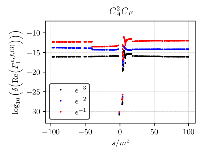
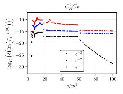
(a)	(b)
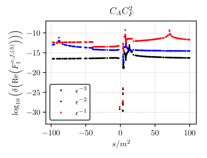
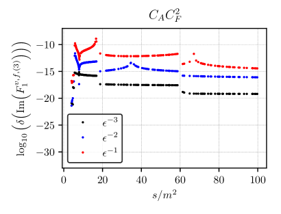
(c)	(d)
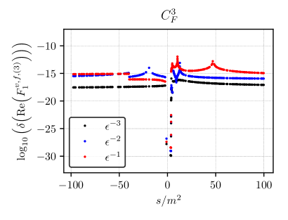
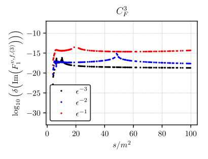
(e)	(f)

Figure 3: Relative cancellation of the real, (a), (c), (e), and imaginary parts, (b), (d), (f), of the poles for the non-fermionic colour structures of $F^{v,f,(3)}_{1}$, c.f. Eq. (31).

Figures for the non-fermionic colour structures of the five remaining form factors can be found in Appendix B. Since the precision of the fermionic colour factors is much better, we refrain from showing the associated plots. In general we observe a progression in the orders of $\epsilon$, i.e. the $1/\epsilon^{-3}$ poles cancel with the highest precision and we lose some digits with every higher order. Sometimes, this general progression is violated, usually if the value of the colour factor changes sign and crosses zero. These zero crossing are visible in the plots, because the precision slowly decreases and then slowly increases again, see for example the region around $s\approx-20m^{2}$ for the real part of the colour factor $C_{F}^{3}$ of $F_{1}^{v,f,(3)}$ in Fig. 3(e).

Let us now analyze the four physical regions $s<0$, $0\leq s<4m^{2}$, $4m^{2}\leq s<16m^{2}$, and $16m^{2}\leq s$ separately in more detail. In each region we provide the minimal precision over all colour factors and form factors. Since the form factors are very small close to zero crossings, we also provide the minimal precision when removing all points for which the size of the coefficient is smaller than $2.5\,\%$ of the average in the region. In addition, we discard all points close to the Coulomb singularity, i.e. $3.95m^{2}\leq s\leq 4.05m^{2}$.

1. In the region $s<0$ we sample over $250$ randomly chosen points for $-100m^{2}\leq s\leq 0$. The poles generally cancel with at least $15$ digits for the $1/\epsilon^{-3}$ poles, at least $10$ digits for the $1/\epsilon^{-2}$ poles, and at least $10$ digits for the $1/\epsilon$ poles. Removing the points close to the zero crossings this improves to $15$, $12$, and $11$ digits, respectively.

2. The region $0\leq s<4m^{2}$ is the most precise one: For the $1000$ random sample points, the poles cancel with at least $17$, $14$, $12$ digits for the $1/\epsilon^{-3}$, $1/\epsilon^{-2}$, $1/\epsilon$ poles, respectively. Removing the points close to zero crossings with the threshold chosen above does not improve the precision. However, these reported worst pole cancellations all belong to the power-log expansion around the two-particle threshold at $s=4m^{2}$. For $0\leq s<3.75m^{2}$ our precision is well beyond $20$ digits as can be seen in the figures.

3. The region $4m^{2}\leq s<16m^{2}$ between the thresholds at $s=4m^{2}$ and $s=16m^{2}$ is least precise: For the $1000$ random sample points, the poles of the real part only cancel with at least $11$, $11$, $8$ digits for the $1/\epsilon^{-3}$, $1/\epsilon^{-2}$, $1/\epsilon$ poles, respectively, and the poles for the imaginary parts with $12$, $6$, $6$ digits. Removing the points close to zero crossings mildly improves the precision of the real part to $13$, $12$, $9$ digits. The imaginary part on the other hand significantly improves to $14$, $11$, $9$ digits.

4. The region $16m^{2}\leq s$ becomes more precise again, since it is matched from $+\infty$. For the $250$ random sample points between $16m^{2}\leq s\leq 100m^{2}$, the poles cancel with at least $14$, $13$, $8$ digits for real parts of the $1/\epsilon^{-3}$, $1/\epsilon^{-2}$, $1/\epsilon$ poles, respectively, and with $15$, $11$, $8$ digits for the imaginary parts. This improves to $14$, $13$, $10$ digits for the real part and to $15$, $11$, $9$ digits for the imaginary part when removing the points close to zero crossings.

Extrapolating these numbers to the finite terms, we expect that our result is correct up to at least $7$ digits away from the zero crossings, with a much better precision for most colour factors and form factors over most parts of the real axis.

We have performed the calculation of the form factors for general QCD gauge parameter $\xi$ and have checked that $\xi$ cancels in the renormalized form factors. Note that the mass counterterm contributions depend on $\xi$ which cancels against the bare three-loop expressions. We have checked the cancellation numerically and observe that the coefficient in front of $\xi$ is of order $10^{-18}$ or smaller in most of the phase space.

After specifying to the large-$N_{C}$ limit via $C_{F}\to N_{C}/2$ and $C_{A}\to N_{C}$ we can compare the $N_{C}^{3}$ terms against the exact results from Ref. [8, 11]. In this limit only about 90 planar master integrals contribute and we observe a significantly increased precision of our result. In fact, in the whole $s/m^{2}$ region we can reproduce the exact result with at least 14 digits. with the exception very close to the singularity at $s=4$. For example, for $s=3.9m^{2}$ and $s=4.1m^{2}$ we have an agreement of about 12 digits.

We observe similar results for the light-fermion colour factors $C_{F}^{2}n_{l}$, $C_{A}C_{F}n_{l}$, $C_{F}n_{h}n_{l}$ and $C_{F}n_{l}^{2}$, which we compare against the exact results from Ref. [11], and the $n_{h}^{2}$ terms where the exact expressions can be found in Ref. [19].

For the singlet contribution there are no $1/\epsilon^{2}$ and $1/\epsilon^{3}$ poles from the counterterms. For the $1/\epsilon$ pole we have a much higher precision as can be seen in Fig. 4 for the colour structures $C_{A}C_{F}T_{F}n_{h}$ and $C_{F}^{2}T_{F}n_{h}$ of $F^{s,f,(3)}_{\text{sing}}$.

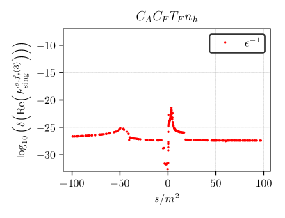
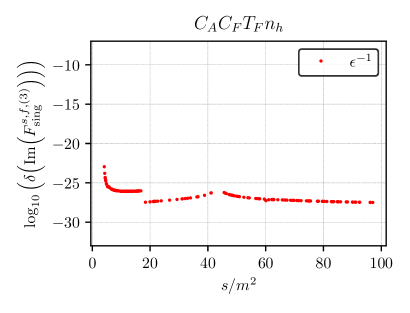
(a)	(b)
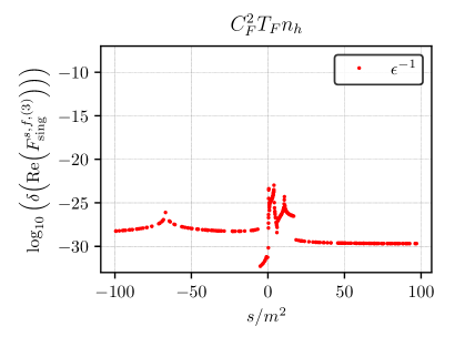
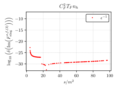
(c)	(d)

Figure 4: Relative cancellation of the real, (a), (c), and imaginary parts, (b), (d), of the poles for the colour structures $C_{A}C_{F}T_{F}n_{h}$ and $C_{F}^{2}T_{F}n_{h}$ of $F^{s,f,(3)}_{\text{sing}}$, c.f. Eq. (31).

We observe that the poles cancel with at least 20 digits, and with several more digits for most regions of the phase space. The cancellation for the other two colour factors with a second fermion loop is even more precise. Due to the high precision we refrain from showing plots for these two colour factors and $F^{p,f,(3)}_{\text{sing}}$. As a conservative estimate we claim a precision of at least 10 digits for the $\epsilon^{0}$ terms of the singlet form factors. Since contributions to $F^{v}_{\text{sing}}$ only start at three-loop order, we cannot check the pole cancellation in this case. However, we do not observe any difference in the behavior of the master integrals which only contribute in this case and, thus, assume the same precision.

6.2 Analytic and numeric expansions

Next we present expansions around the special kinematic points $s=0$ and $s=\pm\infty$. For $s=4m^{2}$ we construct expansions for the cross sections and decay rates, respectively. Such expansions around $s=0,4m^{2}$ and $\infty$ may serve as input for approximation procedures as those based on Padé approximations, see, e.g., Refs. [81, 82, 83].

6.2.1 Static limit: $s\to 0$

In the static limit we construct an analytic expansion including $s^{66}$ from the boundary values at $s=0$. We restrict ourselves again to the five colour structures which are not known analytically. All colour factors as well as higher orders in the expansion are available in the ancillary file accompanying this paper [84]. For illustration we show the results for $F^{v}_{1}$ and $F^{s}$ in the main part of the paper and relegate the remaining four form factors to Appendix C. For the non-singlet form factors the expansions up to $s/m^{2}$ are given by

$$F_{1}^{v,f,(3)}\Big{|}_{s\to 0}=\frac{s}{m^{2}}\Bigg{\{}C_{A}C_{F}^{2}\Bigg{[}\frac{19a_{4}}{2}+\frac{17725\zeta_{3}}{3456}-\frac{\pi^{2}\zeta_{3}}{9}-\frac{55\zeta_{5}}{32}+\frac{707}{288}-\frac{4829\pi^{2}}{10368}-\frac{347\pi^{4}}{17280}$$

$$\quad+\frac{19l_{2}^{4}}{48}-\frac{97}{720}\pi^{2}l_{2}^{2}+\frac{29}{240}\pi^{2}l_{2}\Bigg{]}+C_{A}^{2}C_{F}\Bigg{[}-a_{4}+\frac{4045\zeta_{3}}{5184}+\frac{7\pi^{2}\zeta_{3}}{96}-\frac{5\zeta_{5}}{64}-\frac{7876}{2187}$$

$$\quad+\frac{172285\pi^{2}}{186624}+\frac{67\pi^{4}}{8640}-\frac{l_{2}^{4}}{24}+\frac{67}{360}\pi^{2}l_{2}^{2}-\frac{5131\pi^{2}l_{2}}{2880}\Bigg{]}+C_{F}^{3}\Bigg{[}-15a_{4}-\frac{18367\zeta_{3}}{1728}-\frac{17\pi^{2}\zeta_{3}}{24}$$

$$\quad+\frac{25\zeta_{5}}{8}+\frac{13135}{20736}-\frac{24463\pi^{2}}{7776}+\frac{3037\pi^{4}}{25920}-\frac{5l_{2}^{4}}{8}-\frac{19}{40}\pi^{2}l_{2}^{2}+\frac{4957}{720}\pi^{2}l_{2}\Bigg{]}+C_{F}^{2}T_{F}n_{h}\Bigg{[}-\frac{32a_{4}}{9}$$

$$\quad+\frac{1441\zeta_{3}}{1728}-\frac{2273}{1296}+\frac{1057\pi^{2}}{2430}-\frac{13\pi^{4}}{1620}-\frac{4l_{2}^{4}}{27}+\frac{4}{27}\pi^{2}l_{2}^{2}-\frac{2}{9}\pi^{2}l_{2}\Bigg{]}+C_{F}C_{A}T_{F}n_{h}\Bigg{[}\frac{17a_{4}}{6}$$

$$\quad+\frac{1775\zeta_{3}}{864}-\frac{\pi^{2}\zeta_{3}}{18}+\frac{5\zeta_{5}}{12}-\frac{23089}{5184}+\frac{4813\pi^{2}}{5184}+\frac{803\pi^{4}}{51840}+\frac{17l_{2}^{4}}{144}-\frac{17}{144}\pi^{2}l_{2}^{2}-\frac{149}{108}\pi^{2}l_{2}\Bigg{]}\Bigg{\}}$$

$$\quad+{\cal O}\left(\frac{s^{2}}{m^{4}}\right)+\mbox{$n_{l}$, $n_{l}^{2}$ and $n_{h}^{2}$ terms},$$ (32)

$$F^{s,f,(3)}\Big{|}_{s\to 0}=C_{A}C_{F}^{2}\Bigg{[}\frac{4a_{4}}{3}+\frac{491\zeta_{3}}{96}+\frac{19\pi^{2}\zeta_{3}}{16}-\frac{45\zeta_{5}}{16}+\frac{26117}{4608}-\frac{1193\pi^{2}}{576}-\frac{65\pi^{4}}{432}+\frac{l_{2}^{4}}{18}$$

$$\quad+\frac{31}{36}\pi^{2}l_{2}^{2}+\frac{43}{18}\pi^{2}l_{2}\Bigg{]}+C_{A}^{2}C_{F}\Bigg{[}-\frac{11a_{4}}{3}-\frac{947\zeta_{3}}{288}-\frac{51\pi^{2}\zeta_{3}}{64}+\frac{65\zeta_{5}}{32}-\frac{584447}{124416}+\frac{3011\pi^{2}}{3456}$$

$$\quad+\frac{179\pi^{4}}{3456}-\frac{11l_{2}^{4}}{72}-\frac{11}{36}\pi^{2}l_{2}^{2}+\frac{49}{72}\pi^{2}l_{2}\Bigg{]}+C_{F}^{3}\Bigg{[}12a_{4}+\frac{87\zeta_{3}}{16}+\frac{\pi^{2}\zeta_{3}}{16}-\frac{5\zeta_{5}}{8}+\frac{55}{96}+\frac{643\pi^{2}}{192}$$

$$\quad+\frac{\pi^{4}}{48}+\frac{l_{2}^{4}}{2}-\frac{1}{2}\pi^{2}l_{2}^{2}-\frac{15}{2}\pi^{2}l_{2}\Bigg{]}+C_{F}^{2}T_{F}n_{h}\Bigg{[}8a_{4}+\frac{17\zeta_{3}}{18}-\frac{2083}{432}-\frac{52\pi^{2}}{81}-\frac{\pi^{4}}{720}+\frac{l_{2}^{4}}{3}$$

$$\quad-\frac{1}{3}\pi^{2}l_{2}^{2}+\frac{8}{9}\pi^{2}l_{2}\Bigg{]}+C_{F}C_{A}T_{F}n_{h}\Bigg{[}-6a_{4}-\frac{199\zeta_{3}}{144}+\frac{\pi^{2}\zeta_{3}}{8}-\frac{5\zeta_{5}}{8}+\frac{209857}{15552}-\frac{4351\pi^{2}}{1296}$$

$$\quad-\frac{\pi^{4}}{288}-\frac{l_{2}^{4}}{4}+\frac{1}{4}\pi^{2}l_{2}^{2}+\frac{32}{9}\pi^{2}l_{2}\Bigg{]}$$

$$\quad+\frac{s}{m^{2}}\Bigg{\{}C_{A}C_{F}^{2}\Bigg{[}-\frac{8a_{4}}{9}+\frac{2515\zeta_{3}}{2304}-\frac{29\pi^{2}\zeta_{3}}{144}-\frac{95\zeta_{5}}{48}+\frac{11191}{41472}-\frac{15101\pi^{2}}{62208}+\frac{37\pi^{4}}{4320}-\frac{l_{2}^{4}}{27}$$

$$\quad+\frac{1259\pi^{2}l_{2}^{2}}{2160}+\frac{1409\pi^{2}l_{2}}{1440}\Bigg{]}+C_{A}^{2}C_{F}\Bigg{[}\frac{5a_{4}}{4}+\frac{8675\zeta_{3}}{10368}-\frac{73\pi^{2}\zeta_{3}}{1152}+\frac{125\zeta_{5}}{384}-\frac{851465}{279936}$$

$$\quad+\frac{130417\pi^{2}}{186624}+\frac{689\pi^{4}}{103680}+\frac{5l_{2}^{4}}{96}-\frac{1}{20}\pi^{2}l_{2}^{2}-\frac{12253\pi^{2}l_{2}}{8640}\Bigg{]}+C_{F}^{3}\Bigg{[}-\frac{29a_{4}}{9}-\frac{12401\zeta_{3}}{3456}$$

$$\quad-\frac{67\pi^{2}\zeta_{3}}{288}+\frac{85\zeta_{5}}{32}+\frac{22613}{41472}-\frac{69355\pi^{2}}{31104}+\frac{1727\pi^{4}}{25920}-\frac{29l_{2}^{4}}{216}-\frac{1043\pi^{2}l_{2}^{2}}{1080}+\frac{4013\pi^{2}l_{2}}{1080}\Bigg{]}$$

$$\quad+C_{F}^{2}T_{F}n_{h}\Bigg{[}\frac{8a_{4}}{9}+\frac{9889\zeta_{3}}{6912}-\frac{8059}{5184}-\frac{4261\pi^{2}}{25920}+\frac{7\pi^{4}}{1620}+\frac{\log^{4}(2)}{27}-\frac{1}{27}\pi^{2}l_{2}^{2}+\frac{4}{27}\pi^{2}l_{2}\Bigg{]}$$

$$\quad+C_{F}C_{A}T_{F}n_{h}\Bigg{[}-\frac{5a_{4}}{18}+\frac{1657\zeta_{3}}{1728}+\frac{\pi^{2}\zeta_{3}}{96}+\frac{5\zeta_{5}}{96}+\frac{2257}{3888}-\frac{13663\pi^{2}}{25920}-\frac{121\pi^{4}}{51840}-\frac{5l_{2}^{4}}{432}$$

$$\quad+\frac{5}{432}\pi^{2}l_{2}^{2}+\frac{55}{108}\pi^{2}l_{2}\Bigg{]}\Bigg{\}}+{\cal O}\left(\frac{s^{2}}{m^{4}}\right)+\mbox{$n_{l}$, $n_{l}^{2}$ and $n_{h}^{2}$ terms},$$ (33)

where $l_{2}=\log(2)$, $a_{4}=\mbox{Li}_{4}(1/2)$ and $\zeta_{n}$ is Riemann’s zeta function evaluated at $n$. For $s=0$ our results for $F_{2}^{v}(0)$ and $F_{1}^{a}(0)$ agree with Refs. [85] and [86], respectively. Note that for $s=0$ the cusp anomalous dimension in Eq. (26) vanishes and we have $Z=1$.

The $n_{h}$-singlet contribution to the scalar form factor reads

$$F_{\text{sing}}^{s,f,(3)}\Big{|}_{s\to 0}=C_{A}C_{F}T_{F}n_{h}\Bigg{[}\frac{22a_{4}}{3}+\frac{113\zeta_{3}}{36}-\frac{\pi^{2}\zeta_{3}}{4}+\frac{5\zeta_{5}}{4}-\frac{643}{54}+\frac{466\pi^{2}}{81}+\frac{187\pi^{4}}{4320}+\frac{11l_{2}^{4}}{36}$$

$$\quad-\frac{11}{36}\pi^{2}l_{2}^{2}-\frac{61}{9}\pi^{2}l_{2}\Bigg{]}+C_{F}^{2}T_{F}n_{h}\Bigg{[}-\frac{32a_{4}}{3}+\frac{55\zeta_{3}}{72}+\frac{445}{108}+\frac{517\pi^{2}}{324}-\frac{11\pi^{4}}{270}-\frac{4l_{2}^{4}}{9}+\frac{4}{9}\pi^{2}l_{2}^{2}$$

$$\quad-\frac{22}{9}\pi^{2}l_{2}\Bigg{]}+C_{F}T_{F}^{2}n_{h}^{2}\Bigg{[}-\frac{8\zeta_{3}}{3}+\frac{16}{9}+\frac{26\pi^{2}}{135}\Bigg{]}+C_{F}T_{F}^{2}n_{h}n_{l}\Bigg{[}\frac{20}{9}-\frac{10\pi^{2}}{27}\Bigg{]}$$

$$\quad+\frac{\sqrt{-s}}{m}\Bigg{\{}C_{A}C_{F}T_{F}n_{h}\Bigg{[}\frac{11}{36}\pi^{2}l_{\sqrt{-s}/m}+\frac{\pi^{4}}{72}-\frac{263\pi^{2}}{432}\Bigg{]}+C_{F}^{2}T_{F}n_{h}\Bigg{[}\frac{\pi^{2}}{16}\Bigg{]}+C_{F}T_{F}^{2}n_{h}n_{l}\Bigg{[}\frac{4\pi^{2}}{27}$$

$$\quad-\frac{1}{9}\pi^{2}l_{\sqrt{-s}/m}\Bigg{]}\Bigg{\}}$$

$$\quad{-\frac{s}{m^{2}}}\Bigg{\{}C_{A}C_{F}T_{F}n_{h}\Bigg{[}-\frac{13a_{4}}{10}+\frac{11l_{\sqrt{-s}/m}^{2}}{36}+\frac{1}{18}\pi^{2}l_{\sqrt{-s}/m}-\frac{115l_{\sqrt{-s}/m}}{108}-\frac{5\zeta_{5}}{12}+\frac{\pi^{2}\zeta_{3}}{12}$$

$$\quad-\frac{429\zeta_{3}}{800}-\frac{3661\pi^{4}}{259200}-\frac{12708229\pi^{2}}{6804000}+\frac{2494529}{518400}-\frac{13l_{2}^{4}}{240}+\frac{13}{240}\pi^{2}l_{2}^{2}+\frac{2929\pi^{2}l_{2}}{1350}\Bigg{]}$$

$$\quad+C_{F}^{2}T_{F}n_{h}\Bigg{[}\frac{34a_{4}}{15}+\frac{l_{\sqrt{-s}/m}}{8}+\frac{15083\zeta_{3}}{172800}+\frac{29\pi^{4}}{2400}-\frac{15689483\pi^{2}}{27216000}-\frac{3190951}{1036800}$$

$$\quad+\frac{17l_{2}^{4}}{180}-\frac{17}{180}\pi^{2}l_{2}^{2}+\frac{1417\pi^{2}l_{2}}{1350}\Bigg{]}+C_{F}T_{F}^{2}n_{h}^{2}\Bigg{[}\frac{1531\zeta_{3}}{1728}-\frac{1661}{2592}-\frac{397\pi^{2}}{8505}\Bigg{]}$$

$$\quad+C_{F}T_{F}^{2}n_{h}n_{l}\Bigg{[}-\frac{1}{9}l_{\sqrt{-s}/m}^{2}+\frac{13l_{\sqrt{-s}/m}}{54}+\frac{89\pi^{2}}{972}-\frac{485}{648}\Bigg{]}\Bigg{\}}$$

$$\quad+{\cal O}\left(\frac{\sqrt{-s}^{3}}{m^{3}}\right)\,,$$ (34)

with $l_{\sqrt{-s}/m}=\log(\sqrt{-s}/m)$. This logarithm as well as the expansion in powers of $\sqrt{-s}/m$, instead of $s/m^{2}$ as for the non-singlet contributions show above, originate from the massless cuts through singlet diagrams discussed in Section 4. The results for the vector and pseudo-scalar form factors can be found in Appendix C.

6.2.2 High-energy expansion: $s\to-\infty$

Also for the high-energy expansion we focus on the colour factors $C_{F}^{3}$, $C_{F}^{2}C_{A}$, $C_{F}C_{A}^{2}$, $C_{F}^{2}T_{F}n_{h}$, and $C_{F}C_{A}T_{F}n_{h}$ and refer to the literature [11, 16] for the remaining fermionic contributions. The high-energy expansions of the non-singlet form factors up to $m^{2}/s$ read

$$F_{1}^{v,f,(3)}\Big{|}_{s\to-\infty}=8.3501C_{A}^{2}C_{F}-20.762C_{A}C_{F}^{2}+10.425C_{A}C_{F}T_{F}n_{h}+4.7318C_{F}^{3}$$

$$\quad-3.2872C_{F}^{2}T_{F}n_{h}+\Big{[}-6.3561C_{A}^{2}C_{F}-4.0082C_{A}C_{F}^{2}+7.6917C_{A}C_{F}T_{F}n_{h}+3.4586C_{F}^{3}$$

$$\quad-2.8785C_{F}^{2}T_{F}n_{h}\Big{]}l_{s}+\Big{[}-2.2488C_{A}^{2}C_{F}+0.51078C_{A}C_{F}^{2}+2.2962C_{A}C_{F}T_{F}n_{h}$$

$$\quad+1.4025C_{F}^{3}-1.8900C_{F}^{2}T_{F}n_{h}\Big{]}l_{s}^{2}+\Big{[}-0.42778C_{A}^{2}C_{F}+0.90267C_{A}C_{F}^{2}$$

$$\quad+0.33008C_{A}C_{F}T_{F}n_{h}+0.062184C_{F}^{3}-0.55727C_{F}^{2}T_{F}n_{h}\Big{]}l_{s}^{3}+\Big{[}-0.035012C_{A}^{2}C_{F}$$

$$\quad+0.20814C_{A}C_{F}^{2}+0.025463C_{A}C_{F}T_{F}n_{h}-0.075860C_{F}^{3}-0.086806C_{F}^{2}T_{F}n_{h}\Big{]}l_{s}^{4}$$

$$\quad+\Big{[}0.019097C_{A}C_{F}^{2}-0.023438C_{F}^{3}-0.0069444C_{F}^{2}T_{F}n_{h}\Big{]}l_{s}^{5}+\Big{[}-0.0026042C_{F}^{3}\Big{]}l_{s}^{6}$$

$$\quad+\frac{m^{2}}{-s}\Big{\{}-47.821C_{A}^{2}C_{F}+123.65C_{A}C_{F}^{2}-52.115C_{A}C_{F}T_{F}n_{h}-92.918C_{F}^{3}$$

$$\quad-5.2612C_{F}^{2}T_{F}n_{h}+\Big{[}17.305C_{A}^{2}C_{F}+2.3223C_{A}C_{F}^{2}-25.912C_{A}C_{F}T_{F}n_{h}-10.381C_{F}^{3}$$

$$\quad+3.3633C_{F}^{2}T_{F}n_{h}\Big{]}l_{s}+\Big{[}8.0183C_{A}^{2}C_{F}-19.097C_{A}C_{F}^{2}-7.8739C_{A}C_{F}T_{F}n_{h}+4.9856C_{F}^{3}$$

$$\quad+8.4570C_{F}^{2}T_{F}n_{h}\Big{]}l_{s}^{2}+\Big{[}1.9149C_{A}^{2}C_{F}-6.8519C_{A}C_{F}^{2}-1.4464C_{A}C_{F}T_{F}n_{h}+3.0499C_{F}^{3}$$

$$\quad+2.3758C_{F}^{2}T_{F}n_{h}\Big{]}l_{s}^{3}+\Big{[}0.24069C_{A}^{2}C_{F}-0.91213C_{A}C_{F}^{2}-0.067130C_{A}C_{F}T_{F}n_{h}$$

$$\quad+0.67172C_{F}^{3}+0.48843C_{F}^{2}T_{F}n_{h}\Big{]}l_{s}^{4}+\Big{[}0.0043403C_{A}^{2}C_{F}-0.051389C_{A}C_{F}^{2}$$

$$\quad-0.0034722C_{A}C_{F}T_{F}n_{h}+0.13229C_{F}^{3}+0.0069444C_{F}^{2}T_{F}n_{h}\Big{]}l_{s}^{5}+\Big{[}-0.00052083C_{A}^{2}C_{F}$$

$$\quad-0.0010417C_{A}C_{F}^{2}+0.0041667C_{F}^{3}\Big{]}l_{s}^{6}\Big{\}}+{\cal O}\left(\frac{m^{4}}{(-s)^{2}}\right)+\mbox{$n_{l}$, $n_{l}^{2}$ and $n_{h}^{2}$ terms},$$ (35)

$$F_{2}^{v,f,(3)}\Big{|}_{s\to-\infty}=\frac{m^{2}}{-s}\Big{\{}38.118C_{A}^{2}C_{F}-45.924C_{A}C_{F}^{2}+32.493C_{A}C_{F}T_{F}n_{h}+22.519C_{F}^{3}$$

$$\quad-2.2135C_{F}^{2}T_{F}n_{h}+\Big{[}-6.6042C_{A}^{2}C_{F}-29.110C_{A}C_{F}^{2}+11.444C_{A}C_{F}T_{F}n_{h}+13.611C_{F}^{3}$$

$$\quad+0.099988C_{F}^{2}T_{F}n_{h}\Big{]}l_{s}+\Big{[}0.95557C_{A}^{2}C_{F}-7.0847C_{A}C_{F}^{2}+1.4122C_{A}C_{F}T_{F}n_{h}$$

$$\quad+5.1299C_{F}^{3}-1.2305C_{F}^{2}T_{F}n_{h}\Big{]}l_{s}^{2}+\Big{[}0.31532C_{A}^{2}C_{F}+0.16787C_{A}C_{F}^{2}$$

$$\quad+0.037037C_{A}C_{F}T_{F}n_{h}+0.90641C_{F}^{3}-0.44444C_{F}^{2}T_{F}n_{h}\Big{]}l_{s}^{3}+\Big{[}0.065972C_{A}C_{F}^{2}$$

$$\quad+0.031250C_{F}^{3}-0.069444C_{F}^{2}T_{F}n_{h}\Big{]}l_{s}^{4}+\Big{[}-0.031250C_{F}^{3}\Big{]}l_{s}^{5}\Big{\}}$$

$$\quad+{\cal O}\left(\frac{m^{4}}{(-s)^{2}}\right)+\mbox{$n_{l}$, $n_{l}^{2}$ and $n_{h}^{2}$ terms},$$ (36)

$$F_{1}^{a,f,(3)}\Big{|}_{s\to-\infty}=8.3501C_{A}^{2}C_{F}-20.762C_{A}C_{F}^{2}+10.425C_{A}C_{F}T_{F}n_{h}+4.7318C_{F}^{3}$$

$$\quad-3.2872C_{F}^{2}T_{F}n_{h}+\Big{[}-6.3561C_{A}^{2}C_{F}-4.0082C_{A}C_{F}^{2}+7.6917C_{A}C_{F}T_{F}n_{h}+3.4586C_{F}^{3}$$

$$\quad-2.8785C_{F}^{2}T_{F}n_{h}\Big{]}l_{s}+\Big{[}-2.2488C_{A}^{2}C_{F}+0.51078C_{A}C_{F}^{2}+2.2962C_{A}C_{F}T_{F}n_{h}$$

$$\quad+1.4025C_{F}^{3}-1.8900C_{F}^{2}T_{F}n_{h}\Big{]}l_{s}^{2}+\Big{[}-0.42778C_{A}^{2}C_{F}+0.90267C_{A}C_{F}^{2}$$

$$\quad+0.33008C_{A}C_{F}T_{F}n_{h}+0.062184C_{F}^{3}-0.55727C_{F}^{2}T_{F}n_{h}\Big{]}l_{s}^{3}+\Big{[}-0.035012C_{A}^{2}C_{F}$$

$$\quad+0.20814C_{A}C_{F}^{2}+0.025463C_{A}C_{F}T_{F}n_{h}-0.075860C_{F}^{3}-0.086806C_{F}^{2}T_{F}n_{h}\Big{]}l_{s}^{4}$$

$$\quad+\Big{[}0.019097C_{A}C_{F}^{2}-0.023438C_{F}^{3}-0.0069444C_{F}^{2}T_{F}n_{h}\Big{]}l_{s}^{5}+\Big{[}-0.0026042C_{F}^{3}\Big{]}l_{s}^{6}$$

$$\quad+\frac{m^{2}}{-s}\Big{\{}-57.129C_{A}^{2}C_{F}+113.95C_{A}C_{F}^{2}-59.667C_{A}C_{F}T_{F}n_{h}-59.120C_{F}^{3}$$

$$\quad+8.8792C_{F}^{2}T_{F}n_{h}+\Big{[}10.011C_{A}^{2}C_{F}+41.904C_{A}C_{F}^{2}-35.338C_{A}C_{F}T_{F}n_{h}-39.202C_{F}^{3}$$

$$\quad+13.451C_{F}^{2}T_{F}n_{h}\Big{]}l_{s}+\Big{[}2.2965C_{A}^{2}C_{F}+8.6681C_{A}C_{F}^{2}-9.8312C_{A}C_{F}T_{F}n_{h}-13.759C_{F}^{3}$$

$$\quad+9.8343C_{F}^{2}T_{F}n_{h}\Big{]}l_{s}^{2}+\Big{[}-0.24620C_{A}^{2}C_{F}-0.66843C_{A}C_{F}^{2}-1.3242C_{A}C_{F}T_{F}n_{h}$$

$$\quad-0.50775C_{F}^{3}+1.8351C_{F}^{2}T_{F}n_{h}\Big{]}l_{s}^{3}+\Big{[}-0.064891C_{A}^{2}C_{F}-0.17408C_{A}C_{F}^{2}$$

$$\quad+0.011574C_{A}C_{F}T_{F}n_{h}-0.057746C_{F}^{3}+0.40046C_{F}^{2}T_{F}n_{h}\Big{]}l_{s}^{4}+\Big{[}-0.0085069C_{A}^{2}C_{F}$$

$$\quad+0.022222C_{A}C_{F}^{2}+0.0034722C_{A}C_{F}T_{F}n_{h}+0.067708C_{F}^{3}-0.0069444C_{F}^{2}T_{F}n_{h}\Big{]}l_{s}^{5}$$

$$\quad+\Big{[}0.00052083C_{A}^{2}C_{F}+0.0010417C_{A}C_{F}^{2}-0.0041667C_{F}^{3}\Big{]}l_{s}^{6}\Big{\}}$$

$$\quad+{\cal O}\left(\frac{m^{4}}{(-s)^{2}}\right)+\mbox{$n_{l}$, $n_{l}^{2}$ and $n_{h}^{2}$ terms},$$ (37)

$$F_{2}^{a,f,(3)}\Big{|}_{s\to-\infty}=\frac{m^{2}}{-s}\Big{\{}-5.2743C_{A}^{2}C_{F}+34.122C_{A}C_{F}^{2}+60.378C_{A}C_{F}T_{F}n_{h}+0.51545C_{F}^{3}$$

$$\quad-14.591C_{F}^{2}T_{F}n_{h}+\Big{[}-44.280C_{A}^{2}C_{F}+6.7642C_{A}C_{F}^{2}+32.524C_{A}C_{F}T_{F}n_{h}+8.6355C_{F}^{3}$$

$$\quad-16.414C_{F}^{2}T_{F}n_{h}\Big{]}l_{s}+\Big{[}-9.8090C_{A}^{2}C_{F}+6.8860C_{A}C_{F}^{2}+6.4028C_{A}C_{F}T_{F}n_{h}$$

$$\quad-0.26335C_{F}^{3}-6.2035C_{F}^{2}T_{F}n_{h}\Big{]}l_{s}^{2}+\Big{[}-0.84028C_{A}^{2}C_{F}+4.3484C_{A}C_{F}^{2}$$

$$\quad+0.61111C_{A}C_{F}T_{F}n_{h}-0.32065C_{F}^{3}-1.5556C_{F}^{2}T_{F}n_{h}\Big{]}l_{s}^{3}+\Big{[}0.57292C_{A}C_{F}^{2}-0.34375C_{F}^{3}$$

$$\quad-0.20833C_{F}^{2}T_{F}n_{h}\Big{]}l_{s}^{4}+\Big{[}-0.093750C_{F}^{3}\Big{]}l_{s}^{5}\Big{\}}+{\cal O}\left(\frac{m^{4}}{(-s)^{2}}\right)+\mbox{$n_{l}$, $n_{l}^{2}$ and $n_{h}^{2}$ terms},$$ (38)

$$F^{s,f,(3)}\Big{|}_{s\to-\infty}=25.519C_{A}^{2}C_{F}-16.796C_{A}C_{F}^{2}-3.3697C_{A}C_{F}T_{F}n_{h}-0.82112C_{F}^{3}$$

$$\quad+0.46640C_{F}^{2}T_{F}n_{h}+\Big{[}4.7139C_{A}^{2}C_{F}-5.0600C_{A}C_{F}^{2}-0.43937C_{A}C_{F}T_{F}n_{h}+0.73034C_{F}^{3}$$

$$\quad+2.0176C_{F}^{2}T_{F}n_{h}\Big{]}l_{s}+\Big{[}0.20351C_{A}^{2}C_{F}-2.3029C_{A}C_{F}^{2}+0.69548C_{A}C_{F}T_{F}n_{h}+1.0101C_{F}^{3}$$

$$\quad-0.23908C_{F}^{2}T_{F}n_{h}\Big{]}l_{s}^{2}+\Big{[}-0.21771C_{A}^{2}C_{F}-0.26083C_{A}C_{F}^{2}+0.17730C_{A}C_{F}T_{F}n_{h}$$

$$\quad+0.14235C_{F}^{3}-0.14060C_{F}^{2}T_{F}n_{h}\Big{]}l_{s}^{3}+\Big{[}-0.035012C_{A}^{2}C_{F}+0.064915C_{A}C_{F}^{2}$$

$$\quad+0.025463C_{A}C_{F}T_{F}n_{h}+0.041327C_{F}^{3}-0.034722C_{F}^{2}T_{F}n_{h}\Big{]}l_{s}^{4}+\Big{[}0.019097C_{A}C_{F}^{2}$$

$$\quad-0.0069444C_{F}^{2}T_{F}n_{h}\Big{]}l_{s}^{5}+\Big{[}-0.0026042C_{F}^{3}\Big{]}l_{s}^{6}$$

$$\quad+\frac{m^{2}}{-s}\Big{\{}-40.495C_{A}^{2}C_{F}-37.175C_{A}C_{F}^{2}-33.918C_{A}C_{F}T_{F}n_{h}+32.272C_{F}^{3}$$

$$\quad+1.5879C_{F}^{2}T_{F}n_{h}+\Big{[}31.911C_{A}^{2}C_{F}+5.1716C_{A}C_{F}^{2}-28.235C_{A}C_{F}T_{F}n_{h}-14.201C_{F}^{3}$$

$$\quad+0.60352C_{F}^{2}T_{F}n_{h}\Big{]}l_{s}+\Big{[}6.9504C_{A}^{2}C_{F}+20.896C_{A}C_{F}^{2}-3.5948C_{A}C_{F}T_{F}n_{h}-6.8796C_{F}^{3}$$

$$\quad+0.96287C_{F}^{2}T_{F}n_{h}\Big{]}l_{s}^{2}+\Big{[}0.20466C_{A}^{2}C_{F}-0.065462C_{A}C_{F}^{2}-0.69163C_{A}C_{F}T_{F}n_{h}$$

$$\quad+1.1505C_{F}^{3}-0.24638C_{F}^{2}T_{F}n_{h}\Big{]}l_{s}^{3}+\Big{[}0.052838C_{A}^{2}C_{F}-0.76691C_{A}C_{F}^{2}-0.69218C_{F}^{3}$$

$$\quad+0.27778C_{F}^{2}T_{F}n_{h}\Big{]}l_{s}^{4}+\Big{[}0.12500C_{F}^{3}\Big{]}l_{s}^{5}\Big{\}}+{\cal O}\left(\frac{m^{4}}{(-s)^{2}}\right)+\mbox{$n_{l}$, $n_{l}^{2}$ and $n_{h}^{2}$ terms},$$ (39)

$$F^{p,f,(3)}\Big{|}_{s\to-\infty}=25.519C_{A}^{2}C_{F}-16.796C_{A}C_{F}^{2}-3.3697C_{A}C_{F}T_{F}n_{h}-0.82112C_{F}^{3}$$

$$\quad+0.46640C_{F}^{2}T_{F}n_{h}+\Big{[}4.7139C_{A}^{2}C_{F}-5.0600C_{A}C_{F}^{2}-0.43937C_{A}C_{F}T_{F}n_{h}+0.73034C_{F}^{3}$$

$$\quad+2.0176C_{F}^{2}T_{F}n_{h}\Big{]}l_{s}+\Big{[}0.20351C_{A}^{2}C_{F}-2.3029C_{A}C_{F}^{2}+0.69548C_{A}C_{F}T_{F}n_{h}+1.0101C_{F}^{3}$$

$$\quad-0.23908C_{F}^{2}T_{F}n_{h}\Big{]}l_{s}^{2}+\Big{[}-0.21771C_{A}^{2}C_{F}-0.26083C_{A}C_{F}^{2}+0.17730C_{A}C_{F}T_{F}n_{h}$$

$$\quad+0.14235C_{F}^{3}-0.14060C_{F}^{2}T_{F}n_{h}\Big{]}l_{s}^{3}+\Big{[}-0.035012C_{A}^{2}C_{F}+0.064915C_{A}C_{F}^{2}$$

$$\quad+0.025463C_{A}C_{F}T_{F}n_{h}+0.041327C_{F}^{3}-0.034722C_{F}^{2}T_{F}n_{h}\Big{]}l_{s}^{4}+\Big{[}0.019097C_{A}C_{F}^{2}$$

$$\quad-0.0069444C_{F}^{2}T_{F}n_{h}\Big{]}l_{s}^{5}+\Big{[}-0.0026042C_{F}^{3}\Big{]}l_{s}^{6}$$

$$\quad+\frac{m^{2}}{-s}\Big{\{}-23.466C_{A}^{2}C_{F}+0.55954C_{A}C_{F}^{2}+0.60203C_{A}C_{F}T_{F}n_{h}+50.838C_{F}^{3}$$

$$\quad-0.95432C_{F}^{2}T_{F}n_{h}+\Big{[}10.183C_{A}^{2}C_{F}-15.480C_{A}C_{F}^{2}-11.531C_{A}C_{F}T_{F}n_{h}+7.4435C_{F}^{3}$$

$$\quad+4.5632C_{F}^{2}T_{F}n_{h}\Big{]}l_{s}+\Big{[}4.6124C_{A}^{2}C_{F}+4.9688C_{A}C_{F}^{2}-0.78449C_{A}C_{F}T_{F}n_{h}-9.1395C_{F}^{3}$$

$$\quad+2.5514C_{F}^{2}T_{F}n_{h}\Big{]}l_{s}^{2}+\Big{[}0.17134C_{A}^{2}C_{F}-0.029534C_{A}C_{F}^{2}-0.45089C_{A}C_{F}T_{F}n_{h}$$

$$\quad+1.3184C_{F}^{3}-0.30193C_{F}^{2}T_{F}n_{h}\Big{]}l_{s}^{3}+\Big{[}0.052838C_{A}^{2}C_{F}-0.50996C_{A}C_{F}^{2}-0.19218C_{F}^{3}$$

$$\quad+0.13889C_{F}^{2}T_{F}n_{h}\Big{]}l_{s}^{4}+\Big{[}0.062500C_{F}^{3}\Big{]}l_{s}^{5}\Big{\}}+{\cal O}\left(\frac{m^{4}}{(-s)^{2}}\right)+\mbox{$n_{l}$, $n_{l}^{2}$ and $n_{h}^{2}$ terms},$$ (40)

with $l_{s}=\log(m^{2}/(-s-i\delta))$. The leading logarithmic contributions of order $\alpha_{s}^{n}\log^{2n}(m^{2}/s)$ are given by the Sudakov exponent [87, 88] $\mbox{exp}[-C_{F}\alpha_{s}/(4\pi)\times\log^{2}(m^{2}/s)]$ for $F_{1}^{v,f,(3)}$, $F_{1}^{a,f,(3)}$, $F^{s,f,(3)}$, and $F^{p,f,(3)}$. Our numerical results (shown above with lower precision) are sufficiently precise to reconstruct the analytic coefficient

$$F_{1}^{v,f,(3)}\Big{|}_{m^{0}/(-s)^{0},\,l_{s}^{6}}=F_{1}^{a,f,(3)}\Big{|}_{m^{0}/(-s)^{0},\,l_{s}^{6}}=F^{s,f,(3)}\Big{|}_{m^{0}/(-s)^{0},\,l_{s}^{6}}=F^{p,f,(3)}\Big{|}_{m^{0}/(-s)^{0},\,l_{s}^{6}}=-\frac{C_{F}^{3}}{384}.$$ (41)

Similarly, we can reconstruct the analytic coefficients for the leading logarithms of the first mass corrections and find

$$F_{1}^{v,f,(3)}\Big{|}_{m^{2}/(-s)^{1},\,l_{s}^{6}}=-F_{1}^{a,f,(3)}\Big{|}_{m^{2}/(-s)^{1},\,l_{s}^{6}}=\frac{C_{F}^{3}}{240}-\frac{C_{F}^{2}C_{A}}{960}-\frac{C_{F}C_{A}^{2}}{1920}.$$ (42)

The latter agree with Refs. [89, 90, 91] where the results in Eq. (42) have been obtained using an involved asymptotic expansion of the three-loop vertex diagrams. Moreover, we confirm that there are only subleading contributions from the non-singlet diagrams to the remaining form factors. While $F_{2}^{v,f,(3)}|_{m^{2}/(-s)^{1},\,l_{s}^{6}}$ and $F_{2}^{a,f,(3)}|_{m^{2}/(-s)^{1},\,l_{s}^{6}}$ vanish completely, $F^{s,f,(3)}|_{m^{2}/(-s)^{1},\,l_{s}^{6}}$ and $F^{p,f,(3)}|_{m^{2}/(-s)^{1},\,l_{s}^{6}}$ should receive contributions only through the singlet diagrams which is discussed below.

Our numerical results also allow the reconstruction of the analytic result for the quartic mass corrections of $F_{2}^{v,f,(3)}$ which is given by (not shown in numerical form above)

$$F_{2}^{v,f,(3)}\Big{|}_{m^{4}/(-s)^{2},\,l_{s}^{6}}=-\frac{C_{A}^{2}C_{F}}{180}+\frac{C_{A}C_{F}^{2}}{160}+\frac{7C_{F}^{3}}{720}.$$ (43)

This result disagrees with Ref. [92]. However, we can make both results agree by modifying Eq. (2.14) in Ref. [92] to

$$f(z)=1-\frac{8}{3}\cdot\frac{z}{5}+\dots.$$ (44)

The correctness of our result has been confirmed by the authors of Ref. [92].

Finally, we show the reconstructed analytic coefficients for the remaining leading and first subleading logarithms for the first two terms in the high-energy expansion for all currents:

$$F_{1}^{v,f,(3)}\Big{|}_{m^{0}/(-s)^{0},\,l_{s}^{5}} =\frac{11C_{A}C_{F}^{2}}{576}-\frac{3C_{F}^{3}}{128}-\frac{C_{F}^{2}T_{F}n_{h}}{144}-\frac{C_{F}^{2}T_{F}n_{l}}{144}\,,$$

$$F_{1}^{v,f,(3)}\Big{|}_{m^{2}/(-s)^{1},\,l_{s}^{5}} =\frac{5C_{A}^{2}C_{F}}{1152}-\frac{37C_{A}C_{F}^{2}}{720}-\frac{C_{A}C_{F}T_{F}n_{h}}{288}-\frac{C_{A}C_{F}T_{F}n_{l}}{288}+\frac{127C_{F}^{3}}{960}+\frac{C_{F}^{2}T_{F}n_{h}}{144}$$

$$\quad+\frac{C_{F}^{2}T_{F}n_{l}}{144}\,,$$

$$F_{2}^{v,f,(3)}\Big{|}_{m^{2}/(-s)^{1},\,l_{s}^{5}} =-\frac{C_{F}^{3}}{32}\,,$$

$$F_{2}^{v,f,(3)}\Big{|}_{m^{4}/(-s)^{2},\,l_{s}^{5}} =\frac{13C_{A}^{2}C_{F}}{1440}-\frac{71C_{A}C_{F}^{2}}{360}-\frac{C_{A}C_{F}T_{F}n_{h}}{72}-\frac{C_{A}C_{F}T_{F}n_{l}}{72}+\frac{101C_{F}^{3}}{240}$$

$$\quad+\frac{C_{F}^{2}T_{F}n_{h}}{36}+\frac{C_{F}^{2}T_{F}n_{l}}{36}\,,$$

$$F_{1}^{a,f,(3)}\Big{|}_{m^{0}/(-s)^{0},\,l_{s}^{5}} =\frac{11C_{A}C_{F}^{2}}{576}-\frac{3C_{F}^{3}}{128}-\frac{C_{F}^{2}T_{F}n_{h}}{144}-\frac{C_{F}^{2}T_{F}n_{l}}{144}\,,$$

$$F_{1}^{a,f,(3)}\Big{|}_{m^{2}/(-s)^{1},\,l_{s}^{5}} =-\frac{49C_{A}^{2}C_{F}}{5760}+\frac{C_{A}C_{F}^{2}}{45}+\frac{C_{A}C_{F}T_{F}n_{h}}{288}+\frac{C_{A}C_{F}T_{F}n_{l}}{288}+\frac{13C_{F}^{3}}{192}-\frac{C_{F}^{2}T_{F}n_{h}}{144}$$

$$\quad-\frac{C_{F}^{2}T_{F}n_{l}}{144}\,,$$

$$F_{2}^{a,f,(3)}\Big{|}_{m^{2}/(-s)^{1},\,l_{s}^{5}} =-\frac{3C_{F}^{3}}{32}\,,$$

$$F_{2}^{a,f,(3)}\Big{|}_{m^{4}/(-s)^{2},\,l_{s}^{6}} =\frac{C_{A}^{2}C_{F}}{480}+\frac{C_{A}C_{F}^{2}}{240}-\frac{C_{F}^{3}}{60}\,,$$

$$F_{2}^{a,f,(3)}\Big{|}_{m^{4}/(-s)^{2},\,l_{s}^{5}} =-\frac{49C_{A}^{2}C_{F}}{1440}+\frac{4C_{A}C_{F}^{2}}{45}+\frac{C_{A}C_{F}T_{F}n_{h}}{72}+\frac{C_{A}C_{F}T_{F}n_{l}}{72}+\frac{C_{F}^{3}}{48}-\frac{C_{F}^{2}T_{F}n_{h}}{36}$$

$$\quad-\frac{C_{F}^{2}T_{F}n_{l}}{36}\,,$$

$$F^{s,f,(3)}\Big{|}_{m^{0}/(-s)^{0},\,l_{s}^{5}} =\frac{11C_{A}C_{F}^{2}}{576}-\frac{C_{F}^{2}T_{F}n_{h}}{144}-\frac{C_{F}^{2}T_{F}n_{l}}{144}\,,$$

$$F^{s,f,(3)}\Big{|}_{m^{2}/(-s)^{1},\,l_{s}^{5}} =\frac{C_{F}^{3}}{8}\,,$$

$$F^{p,f,(3)}\Big{|}_{m^{0}/(-s)^{0},\,l_{s}^{5}} =\frac{11C_{A}C_{F}^{2}}{576}-\frac{C_{F}^{2}T_{F}n_{h}}{144}-\frac{C_{F}^{2}T_{F}n_{l}}{144}\,,$$

$$F^{p,f,(3)}\Big{|}_{m^{2}/(-s)^{1},\,l_{s}^{5}} =\frac{C_{F}^{3}}{16}\,.$$ (45)

Apart form the leading and subleading logarithms discussed above, our approach provides the whole tower of logarithms and also higher order contributions in $m^{2}/(-s)$. We estimate the accuracy of the non-logarithmic terms in Eqs. (35)-(40) to ten digits. For the subleading terms the accuracy decreases. Note, however, that we use the $s\to\infty$ expansion only for $|s/m^{2}|\gtrsim 45$ and that $1/45^{3}\approx{\cal O}(10^{-5})$.

For the scalar and pseudo-scalar singlet contributions we obtain the following results for the leading logarithmic contributions of the power-suppressed term

$$F_{\rm sing}^{s,f,(3)}\Big{|}_{m^{2}/(-s),\,l_{s}^{6}}=F_{\rm sing}^{p,f,(3)}\Big{|}_{m^{2}/(-s),\,l_{s}^{6}}=\frac{C_{A}C_{F}T_{F}}{960}+\frac{C_{F}^{2}T_{F}}{240}\,,$$ (46)

which is in agreement with Ref. [91].

6.2.3 Threshold expansions: $s\to 4m^{2}$ and $s\to 16m^{2}$

Let us next discuss the two- and four-particle thresholds at $s=4m^{2}$ and $s=16m^{2}$. Close to the two-particle threshold $F_{1}$ develops the famous Coulomb singularity with negative powers in the velocity of the produced quarks, $\beta=\sqrt{1-4m^{2}/s}$, up to third order multiplied by $\log(\beta)$ terms. In this limit real radiation is suppressed by three powers of $\beta$ and it is thus possible to construct physical quantities from the square of the form factors. For the four currents under consideration we follow Ref. [16] and define

$$R^{v} = \beta\left(|F_{1}^{v}+F_{2}^{v}|^{2}+\frac{|(1-\beta^{2}){F_{1}^{v}+F_{2}^{v}}|^{2}}{2(1-\beta^{2})}\right)\,,$$

$$R^{a} = \beta^{3}|F_{1}^{a}|^{2}\,,$$

$$R^{s} = \beta^{3}|F^{s}|^{2}\,,$$

$$R^{p} = \beta|F^{p}|^{2}\,,$$ (47)

These quantities form building blocks for, e.g., cross sections of heavy quark production in electron-positron annihilation or decay rates for scalar or pseudo-scalar Higgs bosons (see also Ref. [16]). For reference we provide the (exact) leading order results which are given by

$$R^{v,(0)} = \frac{3\beta}{2}\left(1-\frac{\beta^{2}}{3}\right)\,,$$

$$R^{a,(0)} = \beta^{3}\,,$$

$$R^{s,(0)} = \beta^{3}\,,$$

$$R^{p,(0)} = \beta\,,$$ (48)

where we adapt the notation from Eq. (3). We parametrize the QCD corrections to $R^{\delta}$ with the quantities $\Delta^{\delta,(i)}$ which we introduce as

$$R^{\delta} = R^{\delta,(0)}+K_{\delta}\beta^{n_{\delta}}\sum_{i\geq 1}\left(\frac{\alpha_{s}(m)}{\pi}\right)^{i}\Delta^{\delta,(i)}\,,$$ (49)

with $K_{v}=3/2$, $K_{a}=K_{s}=K_{p}=1$, $n_{v}=n_{p}=1$ and $n_{a}=n_{s}=3$. For convenience we set $\mu=m$. In contrast to Ref. [16] we present results parametrized in terms of $\alpha_{s}^{(n_{l})}$ (and not $\alpha_{s}^{(n_{l}+1)}$). Furthermore, for the scalar and pseudo-scalar current we keep the factor $m$ in the definition of the currents (see Eq. (1)) in the $\overline{\rm MS}$ scheme and refrain from transformation to the on-shell scheme. Note that this is the natural choice for Higgs decays where the factor $m$ takes over the role of the Yukawa couplings.

The three leading terms in $\beta$ for the four currents read

$$\Delta^{v,(3)}=\Bigg{\{}C_{F}^{3}\bigg{[}-\frac{32.470}{\beta^{2}}+\frac{1}{\beta}(14.998-32.470l_{2\beta})\bigg{]}+C_{A}C_{F}^{2}\bigg{[}\frac{1}{\beta^{2}}(-29.764l_{2\beta}-7.7703)$$

$$\quad+\frac{1}{\beta}(-12.516l_{2\beta}-11.435)\bigg{]}+C_{A}^{2}C_{F}\bigg{[}\frac{1}{\beta}(16.586l^{2}_{2\beta}-22.572l_{2\beta}+42.936)\bigg{]}+\mathcal{O}(\beta^{0})\Bigg{\}}$$

$$\quad+\Bigg{\{}C_{F}^{2}T_{F}n_{l}\bigg{[}\frac{1}{\beta^{2}}(-1.1101+10.823l_{2\beta})+\frac{1}{\beta}(17.275-10.692l_{2\beta})+10.357+59.345l_{2\beta}$$

$$\quad-4.3865l_{2\beta}^{2}\bigg{]}+C_{A}C_{F}T_{F}n_{l}\bigg{[}\frac{1}{\beta}(-33.609+19.831l_{2\beta}-12.063l_{2\beta}^{2})+52.985+26.593l_{2\beta}$$

$$\quad-6.5797l_{2\beta}^{2}\bigg{]}+C_{F}^{2}T_{F}n_{h}\bigg{[}\frac{2.4792}{\beta}-2.0339-1.3159l_{2\beta}\bigg{]}+C_{A}C_{F}T_{F}n_{h}\bigg{[}-0.20495\bigg{]}$$

$$\quad+C_{F}T_{F}^{2}n_{l}^{2}\bigg{[}\frac{1}{\beta}(5.1308-3.6554l_{2\beta}+2.1932l_{2\beta}^{2})-4.9367\bigg{]}+C_{F}T_{F}^{2}n_{l}n_{h}\bigg{[}-0.54050\bigg{]}$$

$$\quad+C_{F}T_{F}^{2}n_{h}^{2}\bigg{[}0.10248\bigg{]}+\mathcal{O}(\beta^{1})\Bigg{\}}\,,$$ (50)

$$\Delta^{a,(3)}=\Bigg{\{}C_{F}^{3}\bigg{[}\frac{12.176}{\beta^{3}}-\frac{21.170}{\beta^{2}}+\frac{1}{\beta}(64.060-40.587l_{2\beta})\bigg{]}+C_{A}C_{F}^{2}\bigg{[}\frac{1}{\beta^{2}}(48.861-38.811l_{2\beta})$$

$$\quad+\frac{1}{\beta}(-32.967+1.8594l_{2\beta})\bigg{]}+C_{A}^{2}C_{F}\bigg{[}\frac{1}{\beta}(82.095-55.745l_{2\beta}+16.586l_{2\beta}^{2})\bigg{]}+\mathcal{O}(\beta^{0})\Bigg{\}}$$

$$\quad+\Bigg{\{}C_{F}^{2}T_{F}n_{l}\bigg{[}\frac{1}{\beta^{2}}(-22.900+14.113l_{2\beta})+\frac{1}{\beta}(13.711-4.1123l_{2\beta})-22.081+59.937l_{2\beta}$$

$$\quad-5.4831l_{2\beta}^{2}\bigg{]}+C_{A}C_{F}T_{F}n_{l}\bigg{[}\frac{1}{\beta}(-65.503+43.956l_{2\beta}-12.063l_{2\beta}^{2})+24.409+14.713l_{2\beta}$$

$$\quad-2.1932l_{2\beta}^{2}\bigg{]}+C_{F}^{2}T_{F}n_{h}\bigg{[}\frac{0.28599}{\beta}+1.7363\bigg{]}+C_{A}C_{F}T_{F}n_{h}\bigg{[}-0.43382\bigg{]}$$

$$\quad+C_{F}T_{F}^{2}n_{l}^{2}\bigg{[}\frac{1}{\beta}(10.979-8.0419l_{2\beta}+2.1932l_{2\beta}^{2})-2.2646\bigg{]}+C_{F}T_{F}^{2}n_{l}n_{h}\bigg{[}-0.24958\bigg{]}$$

$$\quad+C_{F}T_{F}^{2}n_{h}^{2}\bigg{[}-0.022729\bigg{]}+\mathcal{O}(\beta^{1})\Bigg{\}}\,,$$ (51)

$$\Delta^{s,(3)}=\Bigg{\{}C_{F}^{3}\bigg{[}\frac{12.176}{\beta^{3}}+\frac{10.585}{\beta^{2}}+\frac{1}{\beta}(90.512-64.939l_{2\beta})\bigg{]}+C_{A}C_{F}^{2}\bigg{[}\frac{1}{\beta^{2}}(48.861-38.811l_{2\beta})$$

$$\quad+\frac{1}{\beta}(39.492-25.282l_{2\beta})\bigg{]}+C_{A}^{2}C_{F}\bigg{[}\frac{1}{\beta}(82.095-55.745l_{2\beta}+16.586l_{2\beta}^{2})\bigg{]}+\mathcal{O}(\beta^{0})\Bigg{\}}$$

$$\quad+\Bigg{\{}C_{F}^{2}T_{F}n_{l}\bigg{[}\frac{1}{\beta^{2}}(-22.900+14.113l_{2\beta})+\frac{1}{\beta}(-25.009+5.7573l_{2\beta})-4.5086+69.532l_{2\beta}$$

$$\quad-8.7730l_{2\beta}^{2}\bigg{]}+C_{A}C_{F}T_{F}n_{l}\bigg{[}\frac{1}{\beta}(-65.503+43.956l_{2\beta}-12.063l_{2\beta}^{2})-5.3053+14.713l_{2\beta}$$

$$\quad-2.1932l_{2\beta}^{2}\bigg{]}+C_{F}^{2}T_{F}n_{h}\bigg{[}\frac{2.2364}{\beta}+1.4814\bigg{]}+C_{A}C_{F}T_{F}n_{h}\bigg{[}1.8511\bigg{]}$$

$$\quad+C_{F}T_{F}^{2}n_{l}^{2}\bigg{[}\frac{1}{\beta}(10.979-8.0419l_{2\beta}+2.1932l_{2\beta}^{2})+3.6357\bigg{]}+C_{F}T_{F}^{2}n_{l}n_{h}\bigg{[}-0.087673\bigg{]}$$

$$\quad+C_{F}T_{F}^{2}n_{h}^{2}\bigg{[}0.39896\bigg{]}+\mathcal{O}(\beta^{1})\Bigg{\}}\,,$$ (52)

$$\Delta^{p,(3)}=\Bigg{\{}C_{F}^{3}\bigg{[}-\frac{8.1174}{\beta^{2}}+\frac{1}{\beta}(19.153-97.409l_{2\beta})\bigg{]}+C_{A}C_{F}^{2}\bigg{[}\frac{1}{\beta^{2}}(-7.7703-29.764l_{2\beta})$$

$$\quad+\frac{1}{\beta}(17.393-39.657l_{2\beta})\bigg{]}+C_{A}^{2}C_{F}\bigg{[}\frac{1}{\beta}(42.936-22.572l_{2\beta}+16.586l_{2\beta}^{2})\bigg{]}+\mathcal{O}(\beta^{0})\Bigg{\}}$$

$$\quad+\Bigg{\{}C_{F}^{2}T_{F}n_{l}\bigg{[}\frac{1}{\beta^{2}}(-1.1101+10.823l_{2\beta})+\frac{1}{\beta}(-11.575-0.82247l_{2\beta})+45.228+73.188l_{2\beta}$$

$$\quad-13.159l_{2\beta}^{2}\bigg{]}+C_{A}C_{F}T_{F}n_{l}\bigg{[}\frac{1}{\beta}(-33.609+19.831l_{2\beta}-12.063l_{2\beta}^{2})+27.382+26.593l_{2\beta}$$

$$\quad-6.5797l_{2\beta}^{2}\bigg{]}+C_{F}^{2}T_{F}n_{h}\bigg{[}\frac{4.4296}{\beta}+4.0027-1.3159l_{2\beta}\bigg{]}+C_{A}C_{F}T_{F}n_{h}\bigg{[}0.80851\bigg{]}$$

$$\quad+C_{F}T_{F}^{2}n_{l}^{2}\bigg{[}\frac{1}{\beta}(5.1308-3.6554l_{2\beta}+2.1932l_{2\beta}^{2})+0.96364\bigg{]}+C_{F}T_{F}^{2}n_{l}n_{h}\bigg{[}-0.37860\bigg{]}$$

$$\quad+C_{F}T_{F}^{2}n_{h}^{2}\bigg{[}0.52417\bigg{]}+\mathcal{O}(\beta^{1})\Bigg{\}}\,,$$ (53)

with $l_{2\beta}=\log(2\beta)$. Note that the fermionic contributions are suppressed by one additional power of $\beta$ and, thus, we can show the term $\beta^{0}$ for them in contrast to the non-fermionic contributions. The non-fermionic part of $\Delta^{v,(3)}$ has already been shown in Ref. [21]. In Eqs. (50) to (53) we only show five digits for each coefficient, however, our results for $\Delta^{\delta,(3)}$ contain more significant digits. For example, in the vector and pseudo-scalar case our numerical results reproduce the analytic expressions from Ref. [93] (see also Refs. [94, 83]) with at least 13 digits accuracy. The light-fermion contributions can be compared with the analytic results of Ref. [16] and agreement is found for 19 digits. Similarly, after specifying to the large-$N_{C}$ limit we can reproduce the first 14 digits of Ref. [16] for all four currents.

The four-particle thresholds are much less pronounced in the results for the form factors. For the individual master integrals we observe behaviours of the form $(\beta_{4})^{k}\times\log^{l}(\beta_{4})$ with $k=3$ and $l=5$ where $\beta_{4}=\sqrt{1-16m^{2}/s}$. However, all form factors have a smooth behaviour for $s\to 16m^{2}$. In fact, in all cases there are no $\log(\beta_{4})$ terms in our expansions for $\beta_{4}\to 0$. Furthermore, we observe the first non-analytic terms, i.e. terms where $\beta_{4}$ is raised to an odd power, at order $(\beta_{4})^{7}$ for the axial-vector and scalar form factor and $(\beta_{4})^{9}$ in the vector and pseudo-scalar case. This statement is true both for the non-singlet and singlet form factors. Such a high suppression can partly be explained by the fact that the massive four-particle phase-space, which is one of our master integrals, already provides a factor $(\beta_{4})^{7}$. Due to the more divergent behaviour of the master integrals it is nevertheless necessary to perform a careful matching to $s=16m^{2}$, both from above and below. This means we have to go quite close to $s=16m^{2}$ using Taylor expansions around regular points (in our case we chose $s=15m^{2}$ and $s=17m^{2}$). Furthermore, we constructed 100 terms for the expansion in $\beta_{4}$.

6.3 Numerical results for finite three-loop form factors

For illustration we show in Figs. 5, 6 and 7 the finite non-singlet form factors (see Eq. (30)) for negative $s$, for $0<s<4m^{2}$ and above the two-particle threshold, respectively. Only in the latter case the imaginary parts are different from zero. We restrict ourselves to the non-fermionic colour factors and the contributions containing a closed heavy quark loop. In total we present results for the colour factors $C_{F}^{3}$, $C_{F}^{2}C_{A}$, $C_{F}C_{A}^{2}$, $C_{F}^{2}T_{F}n_{h}$, and $C_{F}C_{A}T_{F}n_{h}$. The remaining fermionic contributions are available in the literature [11, 16, 19]. Our calculations have been performed for general renormalization scale $\mu$; in the plots we choose $\mu^{2}=m^{2}$.

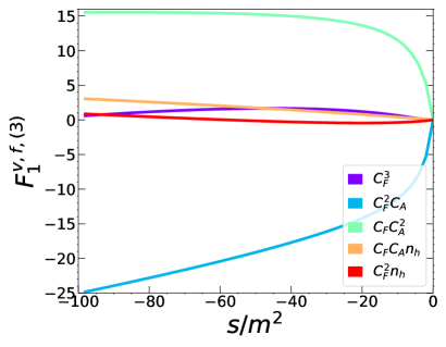
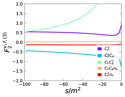
(a)	(b)
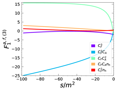
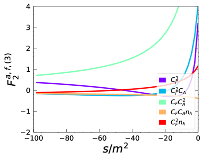
(c)	(d)
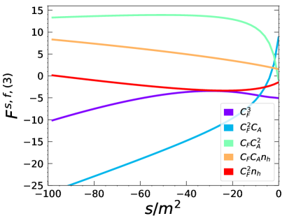
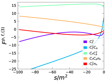
(e)	(f)

Figure 5: Non-singlet form factors as a function of $s$ for $s<0$.

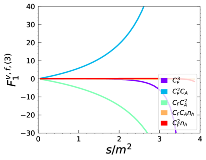
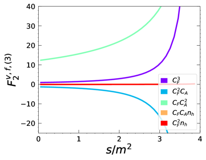
(a)	(b)
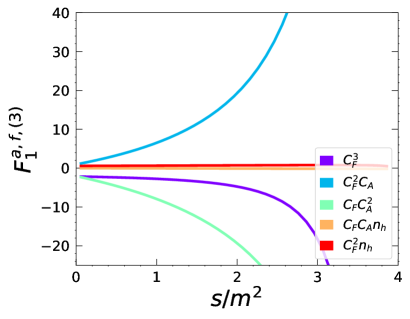
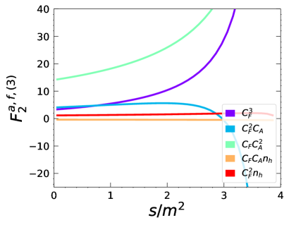
(c)	(d)
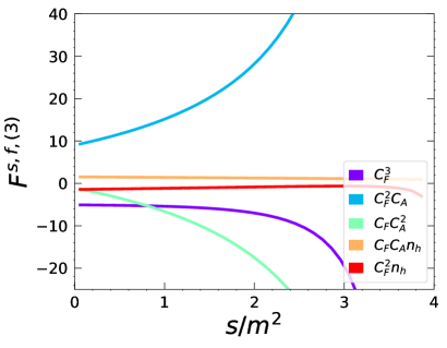
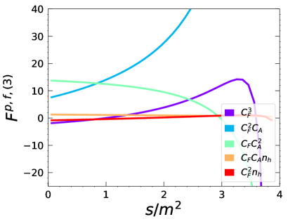
(e)	(f)

Figure 6: Non-singlet form factors as a function of $s$ for $0<s<4m^{2}$.

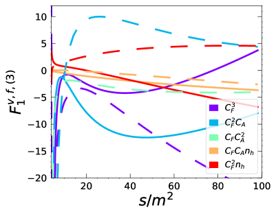
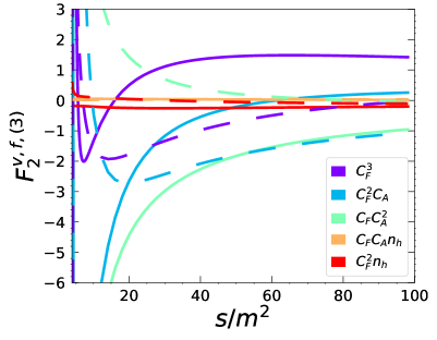
(a)	(b)
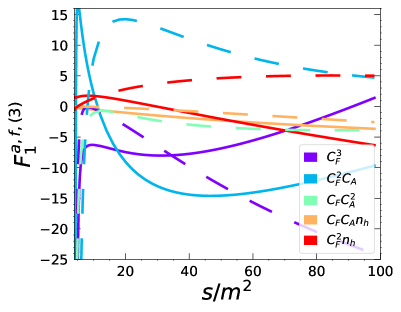
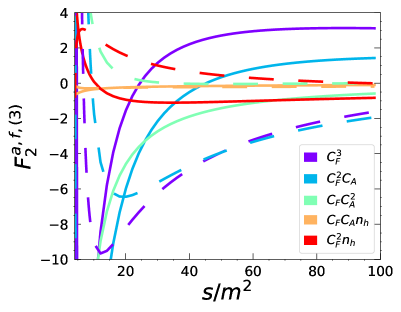
(c)	(d)
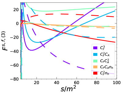
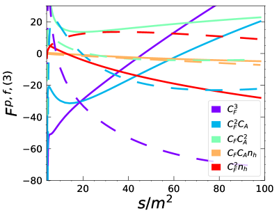
(e)	(f)

Figure 7: Non-singlet form factors as a function of $s$ for $s>4m^{2}$. Real and imaginary parts are shown as solid and dashed lines, respectively.

For $s=0$ we have $F_{1}^{v,f,(3)}=0$ as can be seen in Figs. 5(a) and 6(a), however, the other form factors have in general a finite non-zero value in this limit. For negative $s$ one observes that in general the non-abelian colour structures $C_{F}^{2}C_{A}$ and $C_{F}C_{A}^{2}$ have large coefficients. For the vector and axial-vector contribution the $n_{h}$ terms are numerically smaller whereas for the scalar and pseudo-scalar case they have a similar order of magnitude as the other colour structures.

In Fig. 6 one can clearly see the Coulomb singularities for the non-fermionic contributions close to $s=4m^{2}$. In the $n_{h}$ contributions the closed heavy-quark loop regularizes the $1/\beta$ behaviour and leads to a finite limit for $s\to 4m^{2}$, see also Section 6.2.3.

Fig. 7 shows the results for $s>4m^{2}$ where the form factors develop imaginary parts, see the dashed curves. One again notices the Coulomb singularity on the left part of the plot and the logarithmic behaviour for large values of $s$.

Results for the singlet form factors are shown in Figs. 8, 9 and 10 for the three regions $s<0$, $0<s<4m^{2}$ and $s>4m^{2}$, respectively. In each figure we show plots for the two vector-current form factors and for the scalar and pseudo-scalar currents. Note that non-zero results for the vector form factor are only obtained from the colour factor proportional to $(d^{abc})^{2}$ whereas in the scalar and pseudo-scalar case the other four colour factors have non-zero coefficients.

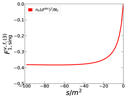
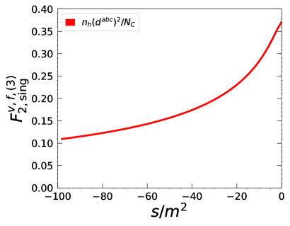
(a)	(b)
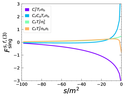
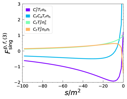
(c)	(d)

Figure 8: Singlet form factors as a function of $s$ for $s<0$.

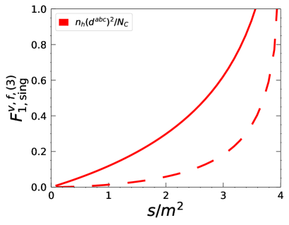
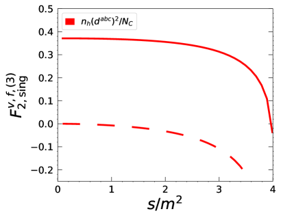
(a)	(b)
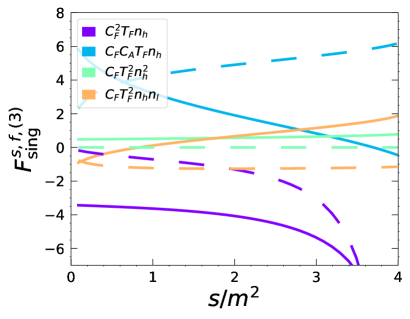
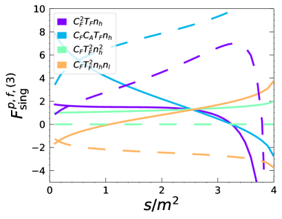
(c)	(d)

Figure 9: Singlet form factors as a function of $s$ for $0<s<4m^{2}$. Real and imaginary parts are shown as solid and dashed lines, respectively.

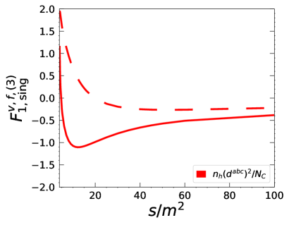
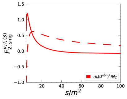
(a)	(b)
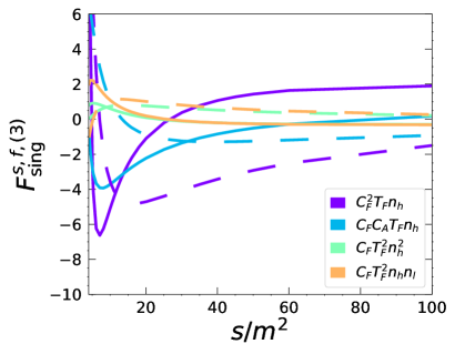
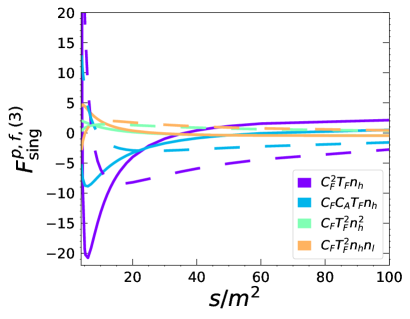
(c)	(d)

Figure 10: Singlet form factors as a function of $s$ for $s>4m^{2}$. Real and imaginary parts are shown as solid and dashed lines, respectively.

It is interesting to note that for $s\to 0$ we have $F_{1,\rm sing}^{v,f,(3)}(0)=0$ and $F_{1,\rm sing}^{v,f,(3)}(0)=\mbox{const}$ whereas the scalar and pseudo-scalar currents behave as $\log^{2}(-s/m^{2})$. The logarithms, which are present in higher expansion terms for all form factors and colour factors, are the reason for the imaginary parts for $s>0$.

The behaviour around $s=4$ is smoother than for the non-singlet form factors. In particular, there are no $1/\beta^{3}$ or $1/\beta^{2}$ singularities. The two vector form factors have a smooth limit and only the colour factor $C_{F}^{2}T_{F}n_{h}$ of the scalar and pseudo-scalar form factors develop $1/\beta$ and $\log(\beta)/\beta$ singularities, both for the real and imaginary parts. The other three colour factors have a finite limit for $s\to 4$.

In the high-energy region all form factors vanish except $F_{1,\rm sing}^{v,f,(3)}$ which approaches a constant. At subleading order there are logarithmic contributions, see also the discussion in Section 6.2.2.

As the central result of this paper we provide a package which allows for the evaluation of both the bare and finite ($F^{f}$) form factors on the publicly accessible webpage [95]. The package is based on expansions combined with interpolations. For the latter we evaluate all six form factors at about 4500 $s/m^{2}$ values.

7 Conclusions

In this paper we compute three-loop corrections to massive quark form factors with external vector, axial-vector, scalar and pseudo-scalar currents and provide precise numerical results in the whole $s/m^{2}$ range. We apply the method developed in Ref. [53] to obtain expansions around regular and singular points. It is based on differential equations which are used to construct the expansions. Two neighboring expansions are numerically matched at an intermediate value of $s$.

We consider both the non-singlet and the singlet contributions, with the restriction that the external currents couple to a closed massive quark loop in the latter case . The main difference between the two contributions is the computation of the boundary conditions at $s=0$. While we have simple Taylor expansions in the non-singlet case, it is necessary to perform an asymptotic expansion for the singlet contributions. Our expansions around $s=0$ are analytic; the expansions around the other $s$ values have precise numeric coefficients. In some cases the precision is sufficient to reconstruct coefficients analytically as, e.g., for leading and sub-leading logarithmic contributions in the high-energy limit. We also provide expansions close to threshold and make the Coulomb singularity explicit.

Our results can be downloaded from the website [95] where an easy-to-use routine is provided which provides numerical results for all six colour factors, both for the singlet and non-singlet contributions. We provide results for each individual colour factor which makes it straightforward to specify to QED.

Appendix A Three-loop on-shell integrals to higher orders in $\epsilon$

For the expansion around $s=0$ we can analytically fix the boundary conditions, since in this case all integrals reduce to massive three-loop on-shell propagators. The most recent calculation of these integrals is given in Ref. [25] and extends to weight 7, formally enough for four-loop calculations. However, since we encounter spurious poles in our reductions of the full system, this is not enough to fix all boundary constants. Some integrals have to be calculated up to weight 9.

A subset of the integrals can be found in the appendix of Ref. [19]. Translating to the notation of Ref. [25] we can fix $I_{12}=G_{45}$, $I_{11}=G_{46}$, and $I_{9}=G_{52}$. But we still need the expansions of the integrals $G_{43}$, $G_{51}$, $G_{53}^{(\star)}$, $G_{61}$, $G_{63}^{(\star)}$, $G_{64}$, $G_{66}$ up to weight 9 (integrals with a $(\star)$ actually only to weight 8). In the following we will describe the steps of the calculation and provide results for all master integrals which cannot be expressed in terms of $\Gamma$-functions up to weight 9.

In a first step we use the Mathematica package Summertime [98] to calculate the needed integrals up to the necessary order in $\epsilon$ with $5000$ digits accuracy, for the integral $G_{8}$ we only obtain with $3000$ digits accuracy. This is the input we use to apply the PSLQ algorithm [99] to fix the analytic form of the expansions. In order to apply this algorithm we need a basis of constants. In all the orders obtained by now, the basis of constants given by harmonic polylogarithms evaluated at argument $1$ was sufficient. We use the basis given in Ref. [100]. This basis is convenient since the harmonic polylogarithms can be calculated to (in principle) arbitrary precision with ginac. For the usage in the PSLQ algorithm we have calculated them with $7500$ digits accuracy. Since we are not dealing with integrals of uniform transcendentality one has to use all products of constants up to the desired weight in the ansatz. Therefore, the number of unknown constants from weight 1 to weight 9 is given by $2$, $4$, $7$, $12$, $20$, $33$, $54$, $88$, $143$. After the successful reconstruction we change to the notation of SUMMER [101]. This has the advantage that most of the transcendental constants are known to Mathematica. The additional constants are given by:

$$s_{6} = S_{0,0,0,0,-1,-1}(\infty)=0.9874414264...~{},$$

$$s_{7a} = S_{0,0,0,0,-1,1,1}(\infty)=-0.9529600758...~{},$$

$$s_{7b} = S_{0,0,0,0,1,-1,-1}(\infty)=1.029121263...~{},$$

$$s_{8a} = S_{0,0,0,0,1,0,0,1}(\infty)=1.041785029...~{},$$

$$s_{8b} = S_{0,0,0,0,0,0,-1,-1}(\infty)=0.9964477484...~{},$$

$$s_{8c} = S_{0,0,0,0,-1,-1,-1,-1}(\infty)=0.9839666738...~{},$$

$$s_{8d} = S_{0,0,0,0,-1,-1,1,1}(\infty)=0.9999626135...~{},$$

$$s_{9a} = S_{0,0,0,0,0,0,1,-1,-1}(\infty)=1.006401963...~{},$$

$$s_{9b} = S_{0,0,0,0,0,0,-1,-1,1}(\infty)=0.9984295251...~{},$$

$$s_{9c} = S_{0,0,0,0,0,-1,0,-1,-1}(\infty)=-0.9874751576...~{},$$

$$s_{9d} = S_{0,0,0,0,-1,-1,1,1,1}(\infty)=1.002198174...~{},$$

$$s_{9e} = S_{0,0,0,0,-1,-1,-1,-1,1}(\infty)=0.9859117196...~{},$$

$$s_{9f} = S_{0,0,0,0,-1,-1,-1,1,-1}(\infty)=0.9784811713...~{}.$$ (54)

Finally, the new results read:

$$G_{43} =\Gamma(1+\epsilon)^{3}\Biggl{\{}\frac{3}{2\epsilon^{3}}+\frac{23}{4\epsilon^{2}}+\frac{105}{8\epsilon}+\frac{275}{16}+\frac{4\pi^{2}}{3}+\epsilon\biggl{(}-\frac{567}{32}+10\pi^{2}-8\pi^{2}l_{2}+28\zeta_{3}\biggr{)}$$

$$+\epsilon^{2}\biggl{(}-\frac{14917}{64}+\frac{145\pi^{2}}{3}-\frac{62\pi^{4}}{45}+192a_{4}-60\pi^{2}l_{2}+16\pi^{2}l_{2}^{2}+8l_{2}^{4}+210\zeta_{3}\biggr{)}$$

$$+\epsilon^{3}\biggl{(}-\frac{144015}{128}+\frac{385\pi^{2}}{2}-\frac{31\pi^{4}}{3}+1440a_{4}+1152a_{5}-290\pi^{2}l_{2}+\frac{124\pi^{4}l_{2}}{15}$$

$$+120\pi^{2}l_{2}^{2}-32\pi^{2}l_{2}^{3}+60l_{2}^{4}-\frac{48l_{2}^{5}}{5}+1015\zeta_{3}-\frac{40}{3}\pi^{2}\zeta_{3}-930\zeta_{5}\biggr{)}+\epsilon^{4}\biggl{(}-\frac{1108525}{256}$$

$$+\frac{8281\pi^{2}}{12}-\frac{899\pi^{4}}{18}-\frac{562\pi^{6}}{135}+6960a_{4}+8640a_{5}+6912a_{6}-1155\pi^{2}l_{2}+62\pi^{4}l_{2}$$

$$+580\pi^{2}l_{2}^{2}-\frac{124}{5}\pi^{4}l_{2}^{2}-240\pi^{2}l_{2}^{3}+290l_{2}^{4}+48\pi^{2}l_{2}^{4}-72l_{2}^{5}+\frac{48l_{2}^{6}}{5}+2880s_{6}$$

$$+\frac{8085\zeta_{3}}{2}-100\pi^{2}\zeta_{3}+80\pi^{2}l_{2}\zeta_{3}-1220\zeta_{3}^{2}-6975\zeta_{5}\biggr{)}+\epsilon^{5}\biggl{(}-\frac{7710087}{512}+\frac{18585\pi^{2}}{8}$$

$$-\frac{2387\pi^{4}}{12}-\frac{281\pi^{6}}{9}+27720a_{4}+41760a_{5}+51840a_{6}+41472a_{7}-\frac{8281}{2}\pi^{2}l_{2}$$

$$+\frac{899\pi^{4}l_{2}}{3}+\frac{784\pi^{6}l_{2}}{45}+2310\pi^{2}l_{2}^{2}-186\pi^{4}l_{2}^{2}-1160\pi^{2}l_{2}^{3}+\frac{248}{5}\pi^{4}l_{2}^{3}+1155l_{2}^{4}$$

$$+360\pi^{2}l_{2}^{4}-348l_{2}^{5}-\frac{288}{5}\pi^{2}l_{2}^{5}+72l_{2}^{6}-\frac{288l_{2}^{7}}{35}+21600s_{6}-\frac{55680}{7}l_{2}s_{6}+\frac{55680s_{7a}}{7}$$

$$-\frac{65280s_{7b}}{7}+\frac{57967\zeta_{3}}{4}-\frac{1450}{3}\pi^{2}\zeta_{3}+\frac{4300\pi^{4}\zeta_{3}}{63}+600\pi^{2}l_{2}\zeta_{3}-240\pi^{2}l_{2}^{2}\zeta_{3}-9150\zeta_{3}^{2}$$

$$+\frac{69600}{7}l_{2}\zeta_{3}^{2}-\frac{67425\zeta_{5}}{2}+\frac{32086\pi^{2}\zeta_{5}}{7}+16740l_{2}^{2}\zeta_{5}-\frac{579651\zeta_{7}}{7}\biggr{)}+\epsilon^{6}\biggl{(}-\frac{50743957}{1024}$$

$$+\frac{360865\pi^{2}}{48}-\frac{256711\pi^{4}}{360}-\frac{8149\pi^{6}}{54}-\frac{429467\pi^{8}}{33075}+99372a_{4}+\frac{1856\pi^{4}a_{4}}{7}$$

$$+166320a_{5}+250560a_{6}+311040a_{7}+248832a_{8}-\frac{55755}{4}\pi^{2}l_{2}+\frac{2387\pi^{4}l_{2}}{2}$$

$$+\frac{392\pi^{6}l_{2}}{3}+8281\pi^{2}l_{2}^{2}-899\pi^{4}l_{2}^{2}+\frac{124}{35}\pi^{6}l_{2}^{2}-4620\pi^{2}l_{2}^{3}+372\pi^{4}l_{2}^{3}+\frac{8281l_{2}^{4}}{2}$$

$$+1740\pi^{2}l_{2}^{4}-\frac{6652}{105}\pi^{4}l_{2}^{4}-1386l_{2}^{5}-432\pi^{2}l_{2}^{5}+348l_{2}^{6}+\frac{288}{5}\pi^{2}l_{2}^{6}-\frac{432l_{2}^{7}}{7}+\frac{216l_{2}^{8}}{35}$$

$$+104400s_{6}-\frac{171840}{7}\pi^{2}s_{6}-\frac{417600}{7}l_{2}s_{6}-\frac{195840}{7}l_{2}^{2}s_{6}+\frac{417600s_{7a}}{7}+\frac{575628s_{8a}}{7}$$

$$-\frac{489600s_{7b}}{7}+\frac{3647232s_{8b}}{7}+\frac{391680s_{8c}}{7}+\frac{334080s_{8d}}{7}+\frac{390285\zeta_{3}}{8}-1925\pi^{2}\zeta_{3}$$

$$+\frac{10750\pi^{4}\zeta_{3}}{21}-\frac{668160}{7}a_{5}\zeta_{3}+2900\pi^{2}l_{2}\zeta_{3}-\frac{37844}{21}\pi^{4}l_{2}\zeta_{3}-1800\pi^{2}l_{2}^{2}\zeta_{3}$$

$$-\frac{5920}{7}\pi^{2}l_{2}^{3}\zeta_{3}+\frac{5568}{7}l_{2}^{5}\zeta_{3}-44225\zeta_{3}^{2}-\frac{214780}{21}\pi^{2}\zeta_{3}^{2}+\frac{522000}{7}l_{2}\zeta_{3}^{2}-\frac{55080}{7}l_{2}^{2}\zeta_{3}^{2}$$

$$-\frac{537075\zeta_{5}}{4}+\frac{240645\pi^{2}\zeta_{5}}{7}-\frac{192816}{7}\pi^{2}l_{2}\zeta_{5}+125550l_{2}^{2}\zeta_{5}+\frac{477156\zeta_{3}\zeta_{5}}{7}$$

$$-\frac{8694765\zeta_{7}}{14}\biggr{)}+\epsilon^{7}\biggl{(}-\frac{323148735}{2048}+\frac{758945\pi^{2}}{32}-\frac{38409\pi^{4}}{16}-\frac{21637\pi^{6}}{36}-\frac{429467\pi^{8}}{4410}$$

$$+334530a_{4}+\frac{13920\pi^{4}a_{4}}{7}+596232a_{5}+\frac{43776\pi^{4}a_{5}}{7}+997920a_{6}+1503360a_{7}$$

$$+1866240a_{8}+1492992a_{9}-\frac{360865}{8}\pi^{2}l_{2}+\frac{256711\pi^{4}l_{2}}{60}+\frac{5684\pi^{6}l_{2}}{9}$$

$$+\frac{12840131\pi^{8}l_{2}}{14700}+\frac{55755}{2}\pi^{2}l_{2}^{2}-\frac{7161}{2}\pi^{4}l_{2}^{2}+\frac{186}{7}\pi^{6}l_{2}^{2}-16562\pi^{2}l_{2}^{3}+1798\pi^{4}l_{2}^{3}$$

$$+\frac{2812}{35}\pi^{6}l_{2}^{3}+\frac{55755l_{2}^{4}}{4}+6930\pi^{2}l_{2}^{4}-\frac{3326}{7}\pi^{4}l_{2}^{4}-\frac{24843l_{2}^{5}}{5}-2088\pi^{2}l_{2}^{5}+\frac{6504}{175}\pi^{4}l_{2}^{5}$$

$$+1386l_{2}^{6}+432\pi^{2}l_{2}^{6}-\frac{2088l_{2}^{7}}{7}-\frac{1728}{35}\pi^{2}l_{2}^{7}+\frac{324l_{2}^{8}}{7}-\frac{144l_{2}^{9}}{35}+415800s_{6}$$

$$-\frac{1288800}{7}\pi^{2}s_{6}-\frac{2018400}{7}l_{2}s_{6}+\frac{2908800}{49}\pi^{2}l_{2}s_{6}-\frac{1468800}{7}l_{2}^{2}s_{6}+\frac{195840}{7}l_{2}^{3}s_{6}$$

$$+\frac{2018400s_{7a}}{7}-\frac{2223360}{49}\pi^{2}s_{7a}+\frac{4317210s_{8a}}{7}-\frac{2840598}{7}l_{2}s_{8a}+\frac{11116416s_{9a}}{7}$$

$$-\frac{2366400s_{7b}}{7}+\frac{3623040}{49}\pi^{2}s_{7b}+\frac{27354240s_{8b}}{7}-\frac{17823360}{7}l_{2}s_{8b}-713856s_{9b}$$

$$+\frac{2937600s_{8c}}{7}-\frac{2970560s_{9c}}{7}+\frac{2505600s_{8d}}{7}+\frac{829440s_{9d}}{7}+\frac{1175040s_{9e}}{7}$$

$$+\frac{2526055\zeta_{3}}{16}-\frac{41405}{6}\pi^{2}\zeta_{3}+\frac{155875\pi^{4}\zeta_{3}}{63}-\frac{27807877\pi^{6}\zeta_{3}}{13230}-\frac{691200}{7}\pi^{2}a_{4}\zeta_{3}$$

$$-\frac{5011200}{7}a_{5}\zeta_{3}-\frac{4008960}{7}a_{6}\zeta_{3}+11550\pi^{2}l_{2}\zeta_{3}-\frac{94610}{7}\pi^{4}l_{2}\zeta_{3}-8700\pi^{2}l_{2}^{2}\zeta_{3}$$

$$+\frac{49814}{7}\pi^{4}l_{2}^{2}\zeta_{3}-\frac{44400}{7}\pi^{2}l_{2}^{3}\zeta_{3}-\frac{19920}{7}\pi^{2}l_{2}^{4}\zeta_{3}+\frac{41760}{7}l_{2}^{5}\zeta_{3}-\frac{5568}{7}l_{2}^{6}\zeta_{3}$$

$$-2258496s_{6}\zeta_{3}-\frac{352275\zeta_{3}^{2}}{2}-\frac{536950}{7}\pi^{2}\zeta_{3}^{2}+\frac{2523000}{7}l_{2}\zeta_{3}^{2}-\frac{2606020}{49}\pi^{2}l_{2}\zeta_{3}^{2}$$

$$-\frac{413100}{7}l_{2}^{2}\zeta_{3}^{2}+\frac{55080}{7}l_{2}^{3}\zeta_{3}^{2}+\frac{1602131\zeta_{3}^{3}}{3}-\frac{3850665\zeta_{5}}{8}+\frac{2326235\pi^{2}\zeta_{5}}{14}$$

$$-\frac{690564211\pi^{4}\zeta_{5}}{5880}+\frac{27820944a_{4}\zeta_{5}}{7}-\frac{1446120}{7}\pi^{2}l_{2}\zeta_{5}+606825l_{2}^{2}\zeta_{5}$$

$$-\frac{1683618}{7}\pi^{2}l_{2}^{2}\zeta_{5}+\frac{1159206}{7}l_{2}^{4}\zeta_{5}+\frac{3578670\zeta_{3}\zeta_{5}}{7}+\frac{22000710}{7}l_{2}\zeta_{3}\zeta_{5}-\frac{84049395\zeta_{7}}{28}$$

$$-\frac{211530187}{392}\pi^{2}\zeta_{7}-\frac{11029569}{7}l_{2}^{2}\zeta_{7}+\frac{648378363\zeta_{9}}{56}\biggr{)}\Biggr{\}}+\mathcal{O}(\epsilon^{9})~{},$$ (55)

$$G_{51} =\Gamma(1+\epsilon)^{3}\Biggl{\{}-\frac{1}{3\epsilon^{3}}-\frac{5}{3\epsilon^{2}}-\frac{1}{\epsilon}\biggl{(}4+\frac{2\pi^{2}}{3}\biggr{)}+\frac{10}{3}-\frac{7\pi^{2}}{3}-\frac{26\zeta_{3}}{3}+\epsilon\biggl{(}\frac{302}{3}-\pi^{2}$$

$$-\frac{35\pi^{4}}{18}-\frac{94\zeta_{3}}{3}\biggr{)}+\epsilon^{2}\biggl{(}734+\frac{101\pi^{2}}{3}-\frac{551\pi^{4}}{90}-20\zeta_{3}-\frac{76}{3}\pi^{2}\zeta_{3}-462\zeta_{5}\biggr{)}+\epsilon^{3}\biggl{(}\frac{12254}{3}$$

$$+\frac{775\pi^{2}}{3}+\frac{28\pi^{4}}{15}-\frac{2353\pi^{6}}{378}+\frac{1232\zeta_{3}}{3}-\frac{236}{3}\pi^{2}\zeta_{3}-\frac{482\zeta_{3}^{2}}{3}-1482\zeta_{5}\biggr{)}+\epsilon^{4}\biggl{(}\frac{60346}{3}$$

$$+1383\pi^{2}+\frac{5249\pi^{4}}{45}-\frac{36031\pi^{6}}{1890}+\frac{9904\zeta_{3}}{3}+32\pi^{2}\zeta_{3}-\frac{3571}{45}\pi^{4}\zeta_{3}-\frac{1510\zeta_{3}^{2}}{3}+252\zeta_{5}$$

$$-894\pi^{2}\zeta_{5}-15307\zeta_{7}\biggr{)}+\epsilon^{5}\biggl{(}92474+\frac{19327\pi^{2}}{3}+\frac{35659\pi^{4}}{45}+\frac{1021\pi^{6}}{105}-\frac{1247749\pi^{8}}{63000}$$

$$-\frac{6984s_{8a}}{5}+18064\zeta_{3}+\frac{4648\pi^{2}\zeta_{3}}{3}-\frac{10817}{45}\pi^{4}\zeta_{3}+172\zeta_{3}^{2}-\frac{1564}{3}\pi^{2}\zeta_{3}^{2}+26976\zeta_{5}$$

$$-2730\pi^{2}\zeta_{5}-18636\zeta_{3}\zeta_{5}-47249\zeta_{7}\biggr{)}+\epsilon^{6}\biggl{(}\frac{1221898}{3}+\frac{84125\pi^{2}}{3}+\frac{11927\pi^{4}}{3}$$

$$+\frac{366544\pi^{6}}{945}-\frac{11341381\pi^{8}}{189000}-\frac{20952s_{8a}}{5}+\frac{256432\zeta_{3}}{3}+\frac{31160\pi^{2}\zeta_{3}}{3}+\frac{2138\pi^{4}\zeta_{3}}{15}$$

$$-\frac{244121}{945}\pi^{6}\zeta_{3}+\frac{29120\zeta_{3}^{2}}{3}-\frac{4724}{3}\pi^{2}\zeta_{3}^{2}-\frac{19732\zeta_{3}^{3}}{9}+186720\zeta_{5}+1452\pi^{2}\zeta_{5}-2587\pi^{4}\zeta_{5}$$

$$-56676\zeta_{3}\zeta_{5}+21318\zeta_{7}-\frac{52885}{2}\pi^{2}\zeta_{7}-\frac{4189826\zeta_{9}}{9}\biggr{)}\Biggr{\}}+\mathcal{O}(\epsilon^{7})~{},$$ (56)

$$G_{53} =\Gamma(1+\epsilon)^{3}\Biggl{\{}-\frac{1}{\epsilon^{3}}-\frac{16}{3\epsilon^{2}}-\frac{16}{\epsilon}-20-\frac{8\pi^{2}}{3}+2\zeta_{3}+\epsilon\biggl{(}\frac{364}{3}-28\pi^{2}-\frac{3\pi^{4}}{10}+16\pi^{2}l_{2}$$

$$-\frac{200\zeta_{3}}{3}\biggr{)}+\epsilon^{2}\biggl{(}1244-188\pi^{2}+\frac{46\pi^{4}}{15}-512a_{4}+168\pi^{2}l_{2}-\frac{80}{3}\pi^{2}l_{2}^{2}-\frac{64l_{2}^{4}}{3}$$

$$-776\zeta_{3}+21\pi^{2}\zeta_{3}-126\zeta_{5}\biggr{)}+\epsilon^{3}\biggl{(}7572-\frac{3100\pi^{2}}{3}+\frac{218\pi^{4}}{5}+\frac{22\pi^{6}}{35}-5376a_{4}$$

$$-144\pi^{2}a_{4}-3072a_{5}+1128\pi^{2}l_{2}-\frac{128}{5}\pi^{4}l_{2}-280\pi^{2}l_{2}^{2}+6\pi^{4}l_{2}^{2}+\frac{160}{3}\pi^{2}l_{2}^{3}$$

$$-224l_{2}^{4}-6\pi^{2}l_{2}^{4}+\frac{128l_{2}^{5}}{5}-5360\zeta_{3}+\frac{332\pi^{2}\zeta_{3}}{3}-126\pi^{2}l_{2}\zeta_{3}+332\zeta_{3}^{2}+1976\zeta_{5}\biggr{)}$$

$$+\epsilon^{4}\biggl{(}\frac{116084}{3}-5084\pi^{2}+\frac{1576\pi^{4}}{5}+\frac{13268\pi^{6}}{945}-36096a_{4}-576\pi^{2}a_{4}-32256a_{5}$$

$$+864\pi^{2}a_{5}-18432a_{6}+6200\pi^{2}l_{2}-\frac{1344}{5}\pi^{4}l_{2}-\frac{28}{15}\pi^{6}l_{2}+864\pi^{2}a_{4}l_{2}$$

$$-1880\pi^{2}l_{2}^{2}+\frac{504}{5}\pi^{4}l_{2}^{2}+560\pi^{2}l_{2}^{3}-24\pi^{4}l_{2}^{3}-1504l_{2}^{4}-104\pi^{2}l_{2}^{4}+\frac{1344l_{2}^{5}}{5}$$

$$+\frac{144}{5}\pi^{2}l_{2}^{5}-\frac{128l_{2}^{6}}{5}-7680s_{6}+2304l_{2}s_{6}-2304s_{7a}-2304s_{7b}-\frac{89392\zeta_{3}}{3}$$

$$+364\pi^{2}\zeta_{3}+\frac{287\pi^{4}\zeta_{3}}{5}-4032a_{4}\zeta_{3}-664\pi^{2}l_{2}\zeta_{3}+546\pi^{2}l_{2}^{2}\zeta_{3}-168l_{2}^{4}\zeta_{3}+\frac{13744\zeta_{3}^{2}}{3}$$

$$-2880l_{2}\zeta_{3}^{2}+25536\zeta_{5}+942\pi^{2}\zeta_{5}-19302\zeta_{7}\biggr{)}+\epsilon^{5}\biggl{(}181108-23380\pi^{2}$$

$$+\frac{26744\pi^{4}}{15}+\frac{38914\pi^{6}}{315}+\frac{1019\pi^{8}}{280}-198400a_{4}-576\pi^{2}a_{4}+\frac{1152\pi^{4}a_{4}}{5}$$

$$-13824a_{4}^{2}-216576a_{5}+3456\pi^{2}a_{5}-193536a_{6}-5184\pi^{2}a_{6}-110592a_{7}$$

$$+30504\pi^{2}l_{2}-\frac{9024}{5}\pi^{4}l_{2}-\frac{7624}{135}\pi^{6}l_{2}+3456\pi^{2}a_{4}l_{2}-5184\pi^{2}a_{5}l_{2}-\frac{31000}{3}\pi^{2}l_{2}^{2}$$

$$+\frac{4152}{5}\pi^{4}l_{2}^{2}-\frac{48}{5}\pi^{6}l_{2}^{2}-1440\pi^{2}a_{4}l_{2}^{2}+3760\pi^{2}l_{2}^{3}-\frac{1248}{5}\pi^{4}l_{2}^{3}-\frac{24800l_{2}^{4}}{3}$$

$$-864\pi^{2}l_{2}^{4}+\frac{198}{5}\pi^{4}l_{2}^{4}-1152a_{4}l_{2}^{4}+\frac{9024l_{2}^{5}}{5}+\frac{1056}{5}\pi^{2}l_{2}^{5}-\frac{1344l_{2}^{6}}{5}-24\pi^{2}l_{2}^{6}$$

$$+\frac{768l_{2}^{7}}{35}-24l_{2}^{8}-80640s_{6}-576\pi^{2}s_{6}+\frac{212992l_{2}s_{6}}{7}-\frac{212992s_{7a}}{7}-4338s_{8a}$$

$$+\frac{109568s_{7b}}{7}-147344\zeta_{3}+872\pi^{2}\zeta_{3}+\frac{13124\pi^{4}\zeta_{3}}{315}-16128a_{4}\zeta_{3}+24192a_{5}\zeta_{3}$$

$$-2184\pi^{2}l_{2}\zeta_{3}+\frac{1008}{5}\pi^{4}l_{2}\zeta_{3}+2664\pi^{2}l_{2}^{2}\zeta_{3}-420\pi^{2}l_{2}^{3}\zeta_{3}-672l_{2}^{4}\zeta_{3}-\frac{1008}{5}l_{2}^{5}\zeta_{3}$$

$$+35488\zeta_{3}^{2}+510\pi^{2}\zeta_{3}^{2}-\frac{266240}{7}l_{2}\zeta_{3}^{2}+180888\zeta_{5}-\frac{178568}{21}\pi^{2}\zeta_{5}+1116\pi^{2}l_{2}\zeta_{5}$$

$$-44640l_{2}^{2}\zeta_{5}-24318\zeta_{3}\zeta_{5}+\frac{1005280\zeta_{7}}{7}\biggr{)}+\epsilon^{6}\biggl{(}805212-\frac{308852\pi^{2}}{3}+\frac{44416\pi^{4}}{5}$$

$$+\frac{246458\pi^{6}}{315}+\frac{1091513\pi^{8}}{22050}-976128a_{4}+6912\pi^{2}a_{4}+\frac{22528\pi^{4}a_{4}}{105}-55296a_{4}^{2}$$

$$-1190400a_{5}+3456\pi^{2}a_{5}+3456\pi^{4}a_{5}-165888a_{4}a_{5}-1299456a_{6}-20736\pi^{2}a_{6}$$

$$-1161216a_{7}+31104\pi^{2}a_{7}-663552a_{8}+140280\pi^{2}l_{2}-9920\pi^{4}l_{2}-\frac{23492}{45}\pi^{6}l_{2}$$

$$+\frac{481517\pi^{8}l_{2}}{500}+3456\pi^{2}a_{4}l_{2}-\frac{32832}{5}\pi^{4}a_{4}l_{2}-20736\pi^{2}a_{5}l_{2}+31104\pi^{2}a_{6}l_{2}$$

$$-50840\pi^{2}l_{2}^{2}+\frac{25632}{5}\pi^{4}l_{2}^{2}-\frac{12664}{315}\pi^{6}l_{2}^{2}-5760\pi^{2}a_{4}l_{2}^{2}+22464\pi^{2}a_{5}l_{2}^{2}$$

$$+\frac{62000}{3}\pi^{2}l_{2}^{3}-\frac{8544}{5}\pi^{4}l_{2}^{3}+\frac{404}{5}\pi^{6}l_{2}^{3}+2880\pi^{2}a_{4}l_{2}^{3}-40672l_{2}^{4}-5352\pi^{2}l_{2}^{4}$$

$$+\frac{113192}{315}\pi^{4}l_{2}^{4}-4608a_{4}l_{2}^{4}-6912a_{5}l_{2}^{4}+9920l_{2}^{5}+\frac{5616}{5}\pi^{2}l_{2}^{5}-\frac{1464}{5}\pi^{4}l_{2}^{5}$$

$$+\frac{6912}{5}a_{4}l_{2}^{5}-\frac{9024l_{2}^{6}}{5}-192\pi^{2}l_{2}^{6}+\frac{1152l_{2}^{7}}{5}-\frac{1056}{35}\pi^{2}l_{2}^{7}-\frac{3936l_{2}^{8}}{35}+\frac{288l_{2}^{9}}{5}$$

$$-541440s_{6}+\frac{442112\pi^{2}s_{6}}{7}+231936l_{2}s_{6}+\frac{293760}{7}\pi^{2}l_{2}s_{6}+\frac{522240}{7}l_{2}^{2}s_{6}$$

$$+48384l_{2}^{3}s_{6}-231936s_{7a}+\frac{165888}{7}\pi^{2}s_{7a}-\frac{1656472s_{8a}}{7}-\frac{2470338}{5}l_{2}s_{8a}$$

$$+2272896s_{9a}+251904s_{7b}+\frac{335232}{7}\pi^{2}s_{7b}+41472l_{2}^{2}s_{7b}-\frac{9725952s_{8b}}{7}$$

$$-3100032l_{2}s_{8b}-1190016s_{9b}-\frac{1044480s_{8c}}{7}-516672s_{9c}-\frac{890880s_{8d}}{7}$$

$$-41472s_{9d}+207360s_{9e}+82944s_{9f}-679088\zeta_{3}+\frac{3784\pi^{2}\zeta_{3}}{3}-\frac{26156}{15}\pi^{4}\zeta_{3}$$

$$-\frac{165286}{35}\pi^{6}\zeta_{3}-16128a_{4}\zeta_{3}+4896\pi^{2}a_{4}\zeta_{3}+\frac{2459136a_{5}\zeta_{3}}{7}+20736a_{6}\zeta_{3}$$

$$-5232\pi^{2}l_{2}\zeta_{3}+\frac{197664}{35}\pi^{4}l_{2}\zeta_{3}+7224\pi^{2}l_{2}^{2}\zeta_{3}-\frac{8886}{5}\pi^{4}l_{2}^{2}\zeta_{3}+\frac{18800}{21}\pi^{2}l_{2}^{3}\zeta_{3}$$

$$-672l_{2}^{4}\zeta_{3}+1266\pi^{2}l_{2}^{4}\zeta_{3}-\frac{102464}{35}l_{2}^{5}\zeta_{3}+\frac{144}{5}l_{2}^{6}\zeta_{3}-2522880s_{6}\zeta_{3}+213424\zeta_{3}^{2}$$

$$+\frac{616520}{21}\pi^{2}\zeta_{3}^{2}-289920l_{2}\zeta_{3}^{2}+\frac{231300}{7}\pi^{2}l_{2}\zeta_{3}^{2}+\frac{146880}{7}l_{2}^{2}\zeta_{3}^{2}+13608l_{2}^{3}\zeta_{3}^{2}$$

$$+\frac{1703845\zeta_{3}^{3}}{3}+1015432\zeta_{5}-125080\pi^{2}\zeta_{5}-\frac{40164351}{280}\pi^{4}\zeta_{5}+5058000a_{4}\zeta_{5}$$

$$+\frac{547440}{7}\pi^{2}l_{2}\zeta_{5}-468720l_{2}^{2}\zeta_{5}-226950\pi^{2}l_{2}^{2}\zeta_{5}+170574l_{2}^{4}\zeta_{5}-\frac{1953320}{7}\zeta_{3}\zeta_{5}$$

$$+3826602l_{2}\zeta_{3}\zeta_{5}+2241396\zeta_{7}-\frac{75881325}{56}\pi^{2}\zeta_{7}-1472679l_{2}^{2}\zeta_{7}+\frac{585155695\zeta_{9}}{24}\biggr{)}\Biggr{\}}$$

$$+\mathcal{O}(\epsilon^{7})~{},$$ (57)

$$G_{61} =\Gamma(1+\epsilon)^{3}\Biggl{\{}\frac{1}{6\epsilon^{3}}+\frac{3}{2\epsilon^{2}}+\frac{1}{\epsilon}\biggl{(}\frac{55}{6}-\frac{\pi^{2}}{3}\biggr{)}+\frac{95}{2}-2\pi^{2}-\frac{8\zeta_{3}}{3}-\frac{\pi^{4}}{15}+\epsilon\biggl{(}\frac{1351}{6}$$

$$-\frac{17\pi^{2}}{3}-\frac{47\pi^{4}}{45}-14\zeta_{3}+6\pi^{2}\zeta_{3}-64\zeta_{5}\biggr{)}+\epsilon^{2}\biggl{(}\frac{2023}{2}+\frac{16\pi^{2}}{3}-\frac{457\pi^{4}}{90}+\frac{1471\pi^{6}}{2835}$$

$$-64\pi^{2}a_{4}-16\pi^{2}l_{2}+\frac{8}{3}\pi^{4}l_{2}^{2}-\frac{8}{3}\pi^{2}l_{2}^{4}+\frac{16\zeta_{3}}{3}+\frac{26\pi^{2}\zeta_{3}}{3}-56\pi^{2}l_{2}\zeta_{3}+62\zeta_{3}^{2}-342\zeta_{5}\biggr{)}$$

$$+\epsilon^{3}\biggr{(}\frac{26335}{6}+187\pi^{2}-\frac{277\pi^{4}}{15}-\frac{299\pi^{6}}{378}+512a_{4}-192\pi^{2}a_{4}+768\pi^{2}a_{5}-224\pi^{2}l_{2}$$

$$-\frac{112}{135}\pi^{6}l_{2}+768\pi^{2}a_{4}l_{2}+\frac{224}{3}\pi^{2}l_{2}^{2}+8\pi^{4}l_{2}^{2}-\frac{64}{3}\pi^{4}l_{2}^{3}+\frac{64l_{2}^{4}}{3}-8\pi^{2}l_{2}^{4}+\frac{128}{5}\pi^{2}l_{2}^{5}$$

$$+1024l_{2}s_{6}-1024s_{7a}-1024s_{7b}+598\zeta_{3}-\frac{58}{3}\pi^{2}\zeta_{3}+\frac{1651\pi^{4}\zeta_{3}}{45}-1792a_{4}\zeta_{3}$$

$$-168\pi^{2}l_{2}\zeta_{3}+\frac{1232}{3}\pi^{2}l_{2}^{2}\zeta_{3}-\frac{224}{3}l_{2}^{4}\zeta_{3}+\frac{400\zeta_{3}^{2}}{3}-1280l_{2}\zeta_{3}^{2}-1082\zeta_{5}$$

$$-\frac{499}{3}\pi^{2}\zeta_{5}-8365\zeta_{7}\biggl{)}+\epsilon^{4}\biggl{(}\frac{37215}{2}+\frac{4598\pi^{2}}{3}-\frac{1195\pi^{4}}{18}-\frac{55943\pi^{6}}{5670}+\frac{1119323\pi^{8}}{243000}$$

$$+7168a_{4}-320\pi^{2}a_{4}+\frac{2752\pi^{4}a_{4}}{15}-12288a_{4}^{2}+6144a_{5}+2304\pi^{2}a_{5}-9216\pi^{2}a_{6}$$

$$-1904\pi^{2}l_{2}+\frac{688\pi^{4}l_{2}}{15}-\frac{112}{45}\pi^{6}l_{2}+2304\pi^{2}a_{4}l_{2}-9216\pi^{2}a_{5}l_{2}+\frac{3136}{3}\pi^{2}l_{2}^{2}$$

$$+\frac{40}{3}\pi^{4}l_{2}^{2}-\frac{344}{45}\pi^{6}l_{2}^{2}-3584\pi^{2}a_{4}l_{2}^{2}-\frac{896}{3}\pi^{2}l_{2}^{3}-64\pi^{4}l_{2}^{3}+\frac{896l_{2}^{4}}{3}-\frac{40}{3}\pi^{2}l_{2}^{4}$$

$$+\frac{3704}{45}\pi^{4}l_{2}^{4}-1024a_{4}l_{2}^{4}-\frac{256l_{2}^{5}}{5}+\frac{384}{5}\pi^{2}l_{2}^{5}-\frac{256}{3}\pi^{2}l_{2}^{6}-\frac{64l_{2}^{8}}{3}-4288\pi^{2}s_{6}$$

$$+3072l_{2}s_{6}-3072s_{7a}+\frac{468s_{8a}}{5}-3072s_{7b}+\frac{17356\zeta_{3}}{3}-\frac{518}{3}\pi^{2}\zeta_{3}+\frac{3692\pi^{4}\zeta_{3}}{45}$$

$$-5376a_{4}\zeta_{3}+21504a_{5}\zeta_{3}-280\pi^{2}l_{2}\zeta_{3}+\frac{2408}{15}\pi^{4}l_{2}\zeta_{3}+1232\pi^{2}l_{2}^{2}\zeta_{3}$$

$$-\frac{3136}{3}\pi^{2}l_{2}^{3}\zeta_{3}-224l_{2}^{4}\zeta_{3}-\frac{896}{5}l_{2}^{5}\zeta_{3}+44\zeta_{3}^{2}+1592\pi^{2}\zeta_{3}^{2}-3840l_{2}\zeta_{3}^{2}-7090\zeta_{5}$$

$$-813\pi^{2}\zeta_{5}+8308\pi^{2}l_{2}\zeta_{5}-19116\zeta_{3}\zeta_{5}-30142\zeta_{7}\biggr{)}+\epsilon^{5}\biggl{(}\frac{465751}{6}+\frac{28331\pi^{2}}{3}$$

$$-\frac{12826\pi^{4}}{45}-\frac{436571\pi^{6}}{5670}+\frac{1941047\pi^{8}}{283500}+60928a_{4}+64\pi^{2}a_{4}+\frac{2752\pi^{4}a_{4}}{5}$$

$$-36864a_{4}^{2}+86016a_{5}+3840\pi^{2}a_{5}+6400\pi^{4}a_{5}-294912a_{4}a_{5}+73728a_{6}$$

$$-27648\pi^{2}a_{6}+110592\pi^{2}a_{7}-12736\pi^{2}l_{2}+\frac{9632\pi^{4}l_{2}}{15}-\frac{112}{27}\pi^{6}l_{2}$$

$$+\frac{13250626\pi^{8}l_{2}}{7875}+3840\pi^{2}a_{4}l_{2}-\frac{57088}{5}\pi^{4}a_{4}l_{2}-27648\pi^{2}a_{5}l_{2}+110592\pi^{2}a_{6}l_{2}$$

$$+\frac{26656}{3}\pi^{2}l_{2}^{2}-\frac{4168}{15}\pi^{4}l_{2}^{2}-\frac{344}{15}\pi^{6}l_{2}^{2}-10752\pi^{2}a_{4}l_{2}^{2}+67584\pi^{2}a_{5}l_{2}^{2}$$

$$-\frac{12544}{3}\pi^{2}l_{2}^{3}-\frac{320}{3}\pi^{4}l_{2}^{3}+\frac{2048}{15}\pi^{6}l_{2}^{3}+14336\pi^{2}a_{4}l_{2}^{3}+\frac{7616l_{2}^{4}}{3}+\frac{2696}{3}\pi^{2}l_{2}^{4}$$

$$+\frac{3704}{15}\pi^{4}l_{2}^{4}-3072a_{4}l_{2}^{4}-12288a_{5}l_{2}^{4}-\frac{3584l_{2}^{5}}{5}+128\pi^{2}l_{2}^{5}-\frac{3328}{5}\pi^{4}l_{2}^{5}$$

$$+\frac{12288}{5}a_{4}l_{2}^{5}+\frac{512l_{2}^{6}}{5}-256\pi^{2}l_{2}^{6}+\frac{17408}{105}\pi^{2}l_{2}^{7}-64l_{2}^{8}+\frac{512l_{2}^{9}}{5}+33792s_{6}$$

$$-12864\pi^{2}s_{6}+5120l_{2}s_{6}+\frac{723456}{7}\pi^{2}l_{2}s_{6}+86016l_{2}^{3}s_{6}-5120s_{7a}$$

$$+\frac{410880}{7}\pi^{2}s_{7a}-\frac{924s_{8a}}{5}-\frac{4391712}{5}l_{2}s_{8a}+4099072s_{9a}-5120s_{7b}$$

$$+\frac{394752}{7}\pi^{2}s_{7b}+73728l_{2}^{2}s_{7b}-5511168l_{2}s_{8b}-2057216s_{9b}-918528s_{9c}$$

$$-73728s_{9d}+368640s_{9e}+147456s_{9f}+39538\zeta_{3}-782\pi^{2}\zeta_{3}+\frac{1762\pi^{4}\zeta_{3}}{45}$$

$$-\frac{23014981\pi^{6}\zeta_{3}}{2835}-8960a_{4}\zeta_{3}+7936\pi^{2}a_{4}\zeta_{3}+64512a_{5}\zeta_{3}+36864a_{6}\zeta_{3}$$

$$+504\pi^{2}l_{2}\zeta_{3}+\frac{2408}{5}\pi^{4}l_{2}\zeta_{3}+\frac{6160}{3}\pi^{2}l_{2}^{2}\zeta_{3}-\frac{45232}{15}\pi^{4}l_{2}^{2}\zeta_{3}-3136\pi^{2}l_{2}^{3}\zeta_{3}$$

$$-\frac{1120}{3}l_{2}^{4}\zeta_{3}+\frac{12704}{3}\pi^{2}l_{2}^{4}\zeta_{3}-\frac{2688}{5}l_{2}^{5}\zeta_{3}+\frac{256}{5}l_{2}^{6}\zeta_{3}-4518144s_{6}\zeta_{3}-\frac{41540\zeta_{3}^{2}}{3}$$

$$+\frac{13796}{3}\pi^{2}\zeta_{3}^{2}-6400l_{2}\zeta_{3}^{2}+\frac{463088}{7}\pi^{2}l_{2}\zeta_{3}^{2}+24192l_{2}^{3}\zeta_{3}^{2}+\frac{3053372\zeta_{3}^{3}}{3}$$

$$-69418\zeta_{5}-\frac{7349}{3}\pi^{2}\zeta_{5}-\frac{15096776}{63}\pi^{4}\zeta_{5}+8899072a_{4}\zeta_{5}+24924\pi^{2}l_{2}\zeta_{5}$$

$$-\frac{1198784}{3}\pi^{2}l_{2}^{2}\zeta_{5}+\frac{898112}{3}l_{2}^{4}\zeta_{5}-63528\zeta_{3}\zeta_{5}+6802848l_{2}\zeta_{3}\zeta_{5}-67226\zeta_{7}$$

$$-\frac{110755595}{42}\pi^{2}\zeta_{7}-2676008l_{2}^{2}\zeta_{7}+\frac{391372085\zeta_{9}}{9}\biggr{)}\Biggr{\}}+\mathcal{O}(\epsilon^{6})~{},$$ (58)

$$G_{62} =\Gamma(1+\epsilon)^{3}\Biggl{\{}\frac{1}{3\epsilon^{3}}+\frac{7}{3\epsilon^{2}}+\frac{31}{3\epsilon}+\frac{103}{3}+\frac{\pi^{2}}{3}-\frac{4\pi^{4}}{45}+\frac{2}{3}\zeta_{3}+\epsilon\biggl{(}\frac{235}{3}+4\pi^{2}-\frac{3\pi^{4}}{10}$$

$$+\frac{20}{3}\zeta_{3}+\frac{2}{3}\pi^{2}\zeta_{3}-2\zeta_{5}\biggr{)}+\epsilon^{2}\biggl{(}\frac{19}{3}+\frac{91\pi^{2}}{3}+\frac{14\pi^{4}}{45}+\frac{1009\pi^{6}}{1890}+\frac{206}{3}\zeta_{3}+2\pi^{2}\zeta_{3}$$

$$+32\zeta_{3}^{2}+6\zeta_{5}-64\pi^{2}a_{4}-16\pi^{2}l_{2}-56\pi^{2}\zeta_{3}l_{2}+\frac{8}{3}\pi^{4}l_{2}^{2}-\frac{8}{3}\pi^{2}l_{2}^{4}\biggr{)}+\epsilon^{3}\biggl{(}-\frac{3953}{3}$$

$$+186\pi^{2}+\frac{307\pi^{4}}{90}+\frac{979\pi^{6}}{630}+\frac{1760}{3}\zeta_{3}+14\pi^{2}\zeta_{3}+\frac{976}{45}\pi^{4}\zeta_{3}+\frac{296}{3}\zeta_{3}^{2}+222\zeta_{5}$$

$$-215\pi^{2}\zeta_{5}-6114\zeta_{7}+512a_{4}-192\pi^{2}a_{4}-1792\zeta_{3}a_{4}+768\pi^{2}a_{5}-224\pi^{2}l_{2}$$

$$-\frac{112}{135}\pi^{6}l_{2}-168\pi^{2}\zeta_{3}l_{2}-1280\zeta_{3}^{2}l_{2}+768\pi^{2}a_{4}l_{2}+\frac{224}{3}\pi^{2}l_{2}^{2}+8\pi^{4}l_{2}^{2}+\frac{1232}{3}\pi^{2}\zeta_{3}l_{2}^{2}$$

$$-\frac{64}{3}\pi^{4}l_{2}^{3}+\frac{64l_{2}^{4}}{3}-8\pi^{2}l_{2}^{4}-\frac{224}{3}\zeta_{3}l_{2}^{4}+\frac{128}{5}\pi^{2}l_{2}^{5}+1024l_{2}s_{6}-1024s_{7a}-1024s_{7b}\biggr{)}$$

$$+\epsilon^{4}\biggl{(}-\frac{31889}{3}+\frac{3025\pi^{2}}{3}-\frac{211\pi^{4}}{15}+\frac{3167\pi^{6}}{630}+\frac{2567\pi^{8}}{500}+\frac{12386}{3}\zeta_{3}+\frac{142}{3}\pi^{2}\zeta_{3}$$

$$+\frac{324}{5}\pi^{4}\zeta_{3}+\frac{752}{3}\zeta_{3}^{2}+\frac{4444}{3}\pi^{2}\zeta_{3}^{2}-3994\zeta_{5}-645\pi^{2}\zeta_{5}-21656\zeta_{3}\zeta_{5}-18176\zeta_{7}$$

$$+7168a_{4}-320\pi^{2}a_{4}+\frac{2752\pi^{4}a_{4}}{15}-5376\zeta_{3}a_{4}-12288a_{4}^{2}+6144a_{5}+2304\pi^{2}a_{5}$$

$$+21504\zeta_{3}a_{5}-9216\pi^{2}a_{6}-1904\pi^{2}l_{2}+\frac{688\pi^{4}l_{2}}{15}-\frac{112}{45}\pi^{6}l_{2}-280\pi^{2}\zeta_{3}l_{2}$$

$$+\frac{2408}{15}\pi^{4}\zeta_{3}l_{2}-3840\zeta_{3}^{2}l_{2}+8308\pi^{2}\zeta_{5}l_{2}+2304\pi^{2}a_{4}l_{2}-9216\pi^{2}a_{5}l_{2}+\frac{3136}{3}\pi^{2}l_{2}^{2}$$

$$+\frac{40}{3}\pi^{4}l_{2}^{2}-\frac{344}{45}\pi^{6}l_{2}^{2}+1232\pi^{2}\zeta_{3}l_{2}^{2}-3584\pi^{2}a_{4}l_{2}^{2}-\frac{896}{3}\pi^{2}l_{2}^{3}-64\pi^{4}l_{2}^{3}-\frac{3136}{3}\pi^{2}\zeta_{3}l_{2}^{3}$$

$$+\frac{896l_{2}^{4}}{3}-\frac{40}{3}\pi^{2}l_{2}^{4}+\frac{3704}{45}\pi^{4}l_{2}^{4}-224\zeta_{3}l_{2}^{4}-1024a_{4}l_{2}^{4}-\frac{256l_{2}^{5}}{5}+\frac{384}{5}\pi^{2}l_{2}^{5}-\frac{896}{5}\zeta_{3}l_{2}^{5}$$

$$-\frac{256}{3}\pi^{2}l_{2}^{6}-\frac{64l_{2}^{8}}{3}-4288\pi^{2}s_{6}+3072l_{2}s_{6}-3072s_{7a}-\frac{2228s_{8a}}{5}-3072s_{7b}\biggr{)}$$

$$+\epsilon^{5}\biggl{(}-\frac{188141}{3}+5048\pi^{2}-\frac{29239\pi^{4}}{90}-\frac{43927\pi^{6}}{1890}+\frac{69049\pi^{8}}{4500}+\frac{75500}{3}\zeta_{3}$$

$$-\frac{550}{3}\pi^{2}\zeta_{3}+\frac{1208}{9}\pi^{4}\zeta_{3}-\frac{856952}{105}\pi^{6}\zeta_{3}-\frac{37768}{3}\zeta_{3}^{2}+4444\pi^{2}\zeta_{3}^{2}+\frac{3051872}{3}\zeta_{3}^{3}$$

$$-71210\zeta_{5}-659\pi^{2}\zeta_{5}-\frac{75528449}{315}\pi^{4}\zeta_{5}-64872\zeta_{3}\zeta_{5}-24070\zeta_{7}-\frac{55362142}{21}\pi^{2}\zeta_{7}$$

$$+43543603\zeta_{9}+60928a_{4}+64\pi^{2}a_{4}+\frac{2752\pi^{4}a_{4}}{5}-8960\zeta_{3}a_{4}+7936\pi^{2}\zeta_{3}a_{4}$$

$$+8899072\zeta_{5}a_{4}-36864a_{4}^{2}+86016a_{5}+3840\pi^{2}a_{5}+6400\pi^{4}a_{5}+64512\zeta_{3}a_{5}$$

$$-294912a_{4}a_{5}+73728a_{6}-27648\pi^{2}a_{6}+36864\zeta_{3}a_{6}+110592\pi^{2}a_{7}-12736\pi^{2}l_{2}$$

$$+\frac{9632\pi^{4}l_{2}}{15}-\frac{112}{27}\pi^{6}l_{2}+\frac{13250626\pi^{8}l_{2}}{7875}+504\pi^{2}\zeta_{3}l_{2}+\frac{2408}{5}\pi^{4}\zeta_{3}l_{2}-6400\zeta_{3}^{2}l_{2}$$

$$+\frac{463088}{7}\pi^{2}\zeta_{3}^{2}l_{2}+24924\pi^{2}\zeta_{5}l_{2}+6802848\zeta_{3}\zeta_{5}l_{2}+3840\pi^{2}a_{4}l_{2}-\frac{57088}{5}\pi^{4}a_{4}l_{2}$$

$$-27648\pi^{2}a_{5}l_{2}+110592\pi^{2}a_{6}l_{2}+\frac{26656}{3}\pi^{2}l_{2}^{2}-\frac{4168}{15}\pi^{4}l_{2}^{2}-\frac{344}{15}\pi^{6}l_{2}^{2}+\frac{6160}{3}\pi^{2}\zeta_{3}l_{2}^{2}$$

$$-\frac{45232}{15}\pi^{4}\zeta_{3}l_{2}^{2}-\frac{1198784}{3}\pi^{2}\zeta_{5}l_{2}^{2}-2676008\zeta_{7}l_{2}^{2}-10752\pi^{2}a_{4}l_{2}^{2}+67584\pi^{2}a_{5}l_{2}^{2}$$

$$-\frac{12544}{3}\pi^{2}l_{2}^{3}-\frac{320}{3}\pi^{4}l_{2}^{3}+\frac{2048}{15}\pi^{6}l_{2}^{3}-3136\pi^{2}\zeta_{3}l_{2}^{3}+24192\zeta_{3}^{2}l_{2}^{3}+14336\pi^{2}a_{4}l_{2}^{3}$$

$$+\frac{7616l_{2}^{4}}{3}+\frac{2696}{3}\pi^{2}l_{2}^{4}+\frac{3704}{15}\pi^{4}l_{2}^{4}-\frac{1120}{3}\zeta_{3}l_{2}^{4}+\frac{12704}{3}\pi^{2}\zeta_{3}l_{2}^{4}+\frac{898112}{3}\zeta_{5}l_{2}^{4}$$

$$-3072a_{4}l_{2}^{4}-12288a_{5}l_{2}^{4}-\frac{3584l_{2}^{5}}{5}+128\pi^{2}l_{2}^{5}-\frac{3328}{5}\pi^{4}l_{2}^{5}-\frac{2688}{5}\zeta_{3}l_{2}^{5}+\frac{12288}{5}a_{4}l_{2}^{5}$$

$$+\frac{512l_{2}^{6}}{5}-256\pi^{2}l_{2}^{6}+\frac{256}{5}\zeta_{3}l_{2}^{6}+\frac{17408}{105}\pi^{2}l_{2}^{7}-64l_{2}^{8}+\frac{512l_{2}^{9}}{5}+33792s_{6}-12864\pi^{2}s_{6}$$

$$-4518144\zeta_{3}s_{6}+5120l_{2}s_{6}+\frac{723456}{7}\pi^{2}l_{2}s_{6}+86016l_{2}^{3}s_{6}-5120s_{7a}+\frac{410880}{7}\pi^{2}s_{7a}$$

$$-\frac{6684s_{8a}}{5}-\frac{4391712}{5}l_{2}s_{8a}+4099072s_{9a}-5120s_{7b}+\frac{394752}{7}\pi^{2}s_{7b}+73728l_{2}^{2}s_{7b}$$

$$-5511168l_{2}s_{8b}-2057216s_{9b}-918528s_{9c}-73728s_{9d}+368640s_{9e}+147456s_{9f}\biggr{)}$$

$$\Biggr{\}}+\mathcal{O}(\epsilon^{6})~{},$$ (59)

$$G_{63} =\Gamma(1+\epsilon)^{3}\Biggl{\{}\frac{1}{6\epsilon^{3}}+\frac{3}{2\epsilon^{2}}+\frac{1}{\epsilon}\biggl{(}\frac{55}{6}-\frac{\pi^{2}}{3}\biggr{)}+\frac{95}{2}-\frac{7\pi^{2}}{3}-\frac{14\zeta_{3}}{3}-\frac{4\pi^{4}}{45}$$

$$+\epsilon\biggl{(}\frac{1351}{6}-\frac{31\pi^{2}}{3}-\frac{23\pi^{4}}{30}+4\pi^{2}l_{2}-42\zeta_{3}+\frac{25\pi^{2}\zeta_{3}}{6}-\frac{49\zeta_{5}}{2}\biggr{)}+\epsilon^{2}\biggl{(}\frac{2023}{2}$$

$$-\frac{103\pi^{2}}{3}-\frac{148\pi^{4}}{45}+\frac{23\pi^{6}}{54}-160a_{4}-56\pi^{2}a_{4}+32\pi^{2}l_{2}-\frac{40}{3}\pi^{2}l_{2}^{2}+\frac{7}{3}\pi^{4}l_{2}^{2}-\frac{20l_{2}^{4}}{3}$$

$$-\frac{7}{3}\pi^{2}l_{2}^{4}-\frac{698\zeta_{3}}{3}+\frac{109\pi^{2}\zeta_{3}}{6}-49\pi^{2}l_{2}\zeta_{3}+\frac{191\zeta_{3}^{2}}{4}-\frac{413\zeta_{5}}{2}\biggr{)}+\epsilon^{3}\biggl{(}\frac{26335}{6}-\frac{235\pi^{2}}{3}$$

$$-\frac{371\pi^{4}}{30}+\frac{457\pi^{6}}{270}-1344a_{4}-280\pi^{2}a_{4}-1472a_{5}+656\pi^{2}a_{5}+140\pi^{2}l_{2}-\frac{182}{45}\pi^{4}l_{2}$$

$$-\frac{35}{54}\pi^{6}l_{2}+656\pi^{2}a_{4}l_{2}-80\pi^{2}l_{2}^{2}+\frac{35}{3}\pi^{4}l_{2}^{2}+\frac{368}{9}\pi^{2}l_{2}^{3}-\frac{164}{9}\pi^{4}l_{2}^{3}-56l_{2}^{4}-\frac{35}{3}\pi^{2}l_{2}^{4}$$

$$+\frac{184l_{2}^{5}}{15}+\frac{328}{15}\pi^{2}l_{2}^{5}+800l_{2}s_{6}-800s_{7a}-800s_{7b}-994\zeta_{3}+\frac{129\pi^{2}\zeta_{3}}{2}+\frac{3803\pi^{4}\zeta_{3}}{180}$$

$$-1400a_{4}\zeta_{3}-245\pi^{2}l_{2}\zeta_{3}+\frac{1036}{3}\pi^{2}l_{2}^{2}\zeta_{3}-\frac{175}{3}l_{2}^{4}\zeta_{3}+\frac{2641\zeta_{3}^{2}}{12}-1000l_{2}\zeta_{3}^{2}+\frac{107\zeta_{5}}{2}$$

$$-\frac{2057}{12}\pi^{2}\zeta_{5}-\frac{44413\zeta_{7}}{8}\biggr{)}+\epsilon^{4}\biggl{(}\frac{37215}{2}-\frac{19\pi^{2}}{3}-\frac{2467\pi^{4}}{45}+\frac{25507\pi^{6}}{1890}+\frac{2351431\pi^{8}}{567000}$$

$$-6496a_{4}-1192\pi^{2}a_{4}+\frac{1580\pi^{4}a_{4}}{9}-9920a_{4}^{2}-10624a_{5}+3280\pi^{2}a_{5}-12928a_{6}$$

$$-8032\pi^{2}a_{6}+328\pi^{2}l_{2}-\frac{124}{45}\pi^{4}l_{2}-\frac{175}{54}\pi^{6}l_{2}+3280\pi^{2}a_{4}l_{2}-8032\pi^{2}a_{5}l_{2}-\frac{280}{3}\pi^{2}l_{2}^{2}$$

$$+\frac{3149}{45}\pi^{4}l_{2}^{2}-\frac{395}{54}\pi^{6}l_{2}^{2}-\frac{9568}{3}\pi^{2}a_{4}l_{2}^{2}+\frac{1504}{9}\pi^{2}l_{2}^{3}-\frac{820}{9}\pi^{4}l_{2}^{3}-\frac{812l_{2}^{4}}{3}-\frac{1255}{9}\pi^{2}l_{2}^{4}$$

$$+\frac{3983}{54}\pi^{4}l_{2}^{4}-\frac{2480}{3}a_{4}l_{2}^{4}+\frac{1328l_{2}^{5}}{15}+\frac{328}{3}\pi^{2}l_{2}^{5}-\frac{808l_{2}^{6}}{45}-\frac{694}{9}\pi^{2}l_{2}^{6}-\frac{155l_{2}^{8}}{9}-4704s_{6}$$

$$-3592\pi^{2}s_{6}+4000l_{2}s_{6}-4000s_{7a}-\frac{1591s_{8a}}{5}-4000s_{7b}-\frac{10346\zeta_{3}}{3}+\frac{1177\pi^{2}\zeta_{3}}{6}$$

$$+\frac{18551\pi^{4}\zeta_{3}}{180}-7000a_{4}\zeta_{3}+17360a_{5}\zeta_{3}-1067\pi^{2}l_{2}\zeta_{3}+\frac{2765}{18}\pi^{4}l_{2}\zeta_{3}+\frac{5180}{3}\pi^{2}l_{2}^{2}\zeta_{3}$$

$$-\frac{8372}{9}\pi^{2}l_{2}^{3}\zeta_{3}-\frac{875}{3}l_{2}^{4}\zeta_{3}-\frac{434}{3}l_{2}^{5}\zeta_{3}+\frac{10741\zeta_{3}^{2}}{4}+\frac{7757}{6}\pi^{2}\zeta_{3}^{2}-5000l_{2}\zeta_{3}^{2}+\frac{5667\zeta_{5}}{2}$$

$$-\frac{10861}{12}\pi^{2}\zeta_{5}+\frac{13919}{2}\pi^{2}l_{2}\zeta_{5}-\frac{66869}{4}\zeta_{3}\zeta_{5}-\frac{231361\zeta_{7}}{8}\biggr{)}+\epsilon^{5}\biggl{(}\frac{465751}{6}+\frac{3953\pi^{2}}{3}$$

$$-\frac{9017\pi^{4}}{30}+\frac{4567\pi^{6}}{70}+\frac{455579\pi^{8}}{22680}-20736a_{4}-5048\pi^{2}a_{4}+\frac{7900\pi^{4}a_{4}}{9}-49600a_{4}^{2}$$

$$-35392a_{5}+11440\pi^{2}a_{5}+\frac{46856\pi^{4}a_{5}}{9}-250112a_{4}a_{5}-71936a_{6}$$

$$-40160\pi^{2}a_{6}-110336a_{7}+99392\pi^{2}a_{7}-636\pi^{2}l_{2}+\frac{12278\pi^{4}l_{2}}{45}-\frac{13331}{210}\pi^{6}l_{2}$$

$$+\frac{119841319\pi^{8}l_{2}}{84000}+12464\pi^{2}a_{4}l_{2}-\frac{445712}{45}\pi^{4}a_{4}l_{2}-40160\pi^{2}a_{5}l_{2}+99392\pi^{2}a_{6}l_{2}$$

$$+2080\pi^{2}l_{2}^{2}+\frac{7693}{45}\pi^{4}l_{2}^{2}-\frac{1975}{54}\pi^{6}l_{2}^{2}-\frac{47840}{3}\pi^{2}a_{4}l_{2}^{2}+\frac{180352}{3}\pi^{2}a_{5}l_{2}^{2}-\frac{7280}{9}\pi^{2}l_{2}^{3}$$

$$-\frac{57088}{135}\pi^{4}l_{2}^{3}+\frac{98777}{810}\pi^{6}l_{2}^{3}+\frac{117824}{9}\pi^{2}a_{4}l_{2}^{3}-864l_{2}^{4}-\frac{2933}{9}\pi^{2}l_{2}^{4}+\frac{19915}{54}\pi^{4}l_{2}^{4}$$

$$-\frac{12400}{3}a_{4}l_{2}^{4}-\frac{31264}{3}a_{5}l_{2}^{4}+\frac{4424l_{2}^{5}}{15}+\frac{25976}{45}\pi^{2}l_{2}^{5}-\frac{79303}{135}\pi^{4}l_{2}^{5}+\frac{31264}{15}a_{4}l_{2}^{5}$$

$$-\frac{4496l_{2}^{6}}{45}-\frac{3470}{9}\pi^{2}l_{2}^{6}+\frac{6896l_{2}^{7}}{315}+\frac{153872}{945}\pi^{2}l_{2}^{7}-\frac{775l_{2}^{8}}{9}+\frac{3908l_{2}^{9}}{45}-19392s_{6}$$

$$-17960\pi^{2}s_{6}+\frac{241376l_{2}s_{6}}{7}+\frac{1847792}{21}\pi^{2}l_{2}s_{6}+\frac{218848}{3}l_{2}^{3}s_{6}-\frac{241376s_{7a}}{7}$$

$$+\frac{1058272}{21}\pi^{2}s_{7a}-1591s_{8a}-\frac{14898273}{20}l_{2}s_{8a}+3476912s_{9a}+\frac{42208s_{7b}}{7}$$

$$+\frac{997232}{21}\pi^{2}s_{7b}+62528l_{2}^{2}s_{7b}-4673968l_{2}s_{8b}-1744176s_{9b}-\frac{2336984s_{9c}}{3}$$

$$-62528s_{9d}+312640s_{9e}+125056s_{9f}-9218\zeta_{3}+\frac{817\pi^{2}\zeta_{3}}{2}+\frac{325943\pi^{4}\zeta_{3}}{1260}$$

$$-\frac{104344579\pi^{6}\zeta_{3}}{15120}-28648a_{4}\zeta_{3}+\frac{20960}{3}\pi^{2}a_{4}\zeta_{3}+86800a_{5}\zeta_{3}+31264a_{6}\zeta_{3}$$

$$-4273\pi^{2}l_{2}\zeta_{3}+\frac{13825}{18}\pi^{4}l_{2}\zeta_{3}+\frac{21692}{3}\pi^{2}l_{2}^{2}\zeta_{3}-\frac{479699}{180}\pi^{4}l_{2}^{2}\zeta_{3}-\frac{41860}{9}\pi^{2}l_{2}^{3}\zeta_{3}$$

$$-\frac{3581}{3}l_{2}^{4}\zeta_{3}+\frac{34256}{9}\pi^{2}l_{2}^{4}\zeta_{3}-\frac{2170}{3}l_{2}^{5}\zeta_{3}+\frac{1954}{45}l_{2}^{6}\zeta_{3}-3828168s_{6}\zeta_{3}+\frac{130813\zeta_{3}^{2}}{12}$$

$$+\frac{12907}{2}\pi^{2}\zeta_{3}^{2}-\frac{301720}{7}l_{2}\zeta_{3}^{2}+\frac{1184933}{21}\pi^{2}l_{2}\zeta_{3}^{2}+20517l_{2}^{3}\zeta_{3}^{2}+\frac{6894063\zeta_{3}^{3}}{8}-\frac{1281\zeta_{5}}{2}$$

$$-\frac{1111457}{84}\pi^{2}\zeta_{5}-\frac{1364278829\pi^{4}\zeta_{5}}{6720}+7555066a_{4}\zeta_{5}+\frac{69595}{2}\pi^{2}l_{2}\zeta_{5}-39246l_{2}^{2}\zeta_{5}$$

$$-\frac{4070633}{12}\pi^{2}l_{2}^{2}\zeta_{5}+\frac{3050645}{12}l_{2}^{4}\zeta_{5}-\frac{337033}{4}\zeta_{3}\zeta_{5}+\frac{23077717}{4}l_{2}\zeta_{3}\zeta_{5}+\frac{4815827\zeta_{7}}{56}$$

$$-\frac{3014004103\pi^{2}\zeta_{7}}{1344}-\frac{18160169}{8}l_{2}^{2}\zeta_{7}+\frac{21258293207\zeta_{9}}{576}\biggr{)}\Biggr{\}}+\mathcal{O}(\epsilon^{6})~{},$$ (60)

$$G_{64} =\Gamma(1+\epsilon)^{3}\Biggl{\{}\frac{2\zeta_{3}}{\epsilon}+2\zeta_{3}+\frac{\pi^{2}}{3}-\frac{7\pi^{4}}{90}+\epsilon\biggl{(}\frac{14\pi^{2}}{3}-\frac{41\pi^{4}}{90}-12\zeta_{3}-\frac{2}{3}\pi^{2}\zeta_{3}+44\zeta_{5}\biggr{)}$$

$$+\epsilon^{2}\biggl{(}\frac{119\pi^{2}}{3}-\frac{14\pi^{4}}{45}+\frac{1447\pi^{6}}{2835}-64\pi^{2}a_{4}-16\pi^{2}l_{2}+\frac{8}{3}\pi^{4}l_{2}^{2}-\frac{8}{3}\pi^{2}l_{2}^{4}-38\zeta_{3}$$

$$-\frac{26}{3}\pi^{2}\zeta_{3}-56\pi^{2}l_{2}\zeta_{3}+54\zeta_{3}^{2}-42\zeta_{5}\biggr{)}+\epsilon^{3}\biggl{(}\frac{796\pi^{2}}{3}+\frac{51\pi^{4}}{10}+\frac{31\pi^{6}}{630}+512a_{4}$$

$$-192\pi^{2}a_{4}+768\pi^{2}a_{5}-224\pi^{2}l_{2}-\frac{112}{135}\pi^{6}l_{2}+768\pi^{2}a_{4}l_{2}+\frac{224}{3}\pi^{2}l_{2}^{2}+8\pi^{4}l_{2}^{2}$$

$$-\frac{64}{3}\pi^{4}l_{2}^{3}+\frac{64l_{2}^{4}}{3}-8\pi^{2}l_{2}^{4}+\frac{128}{5}\pi^{2}l_{2}^{5}+1024l_{2}s_{6}-1024s_{7a}-1024s_{7b}+256\zeta_{3}$$

$$-26\pi^{2}\zeta_{3}+\frac{931\pi^{4}\zeta_{3}}{45}-1792a_{4}\zeta_{3}-168\pi^{2}l_{2}\zeta_{3}+\frac{1232}{3}\pi^{2}l_{2}^{2}\zeta_{3}-\frac{224}{3}l_{2}^{4}\zeta_{3}+104\zeta_{3}^{2}$$

$$-1280l_{2}\zeta_{3}^{2}-574\zeta_{5}-217\pi^{2}\zeta_{5}-5655\zeta_{7}\biggr{)}+\epsilon^{4}\biggl{(}1539\pi^{2}+\frac{331\pi^{4}}{15}-\frac{10667\pi^{6}}{5670}$$

$$+\frac{8360501\pi^{8}}{1701000}+7168a_{4}-320\pi^{2}a_{4}+\frac{2752\pi^{4}a_{4}}{15}-12288a_{4}^{2}+6144a_{5}+2304\pi^{2}a_{5}$$

$$-9216\pi^{2}a_{6}-1904\pi^{2}l_{2}+\frac{688\pi^{4}l_{2}}{15}-\frac{112}{45}\pi^{6}l_{2}+2304\pi^{2}a_{4}l_{2}-9216\pi^{2}a_{5}l_{2}$$

$$+\frac{3136}{3}\pi^{2}l_{2}^{2}+\frac{40}{3}\pi^{4}l_{2}^{2}-\frac{344}{45}\pi^{6}l_{2}^{2}-3584\pi^{2}a_{4}l_{2}^{2}-\frac{896}{3}\pi^{2}l_{2}^{3}-64\pi^{4}l_{2}^{3}+\frac{896l_{2}^{4}}{3}$$

$$-\frac{40}{3}\pi^{2}l_{2}^{4}+\frac{3704}{45}\pi^{4}l_{2}^{4}-1024a_{4}l_{2}^{4}-\frac{256l_{2}^{5}}{5}+\frac{384}{5}\pi^{2}l_{2}^{5}-\frac{256}{3}\pi^{2}l_{2}^{6}-\frac{64l_{2}^{8}}{3}$$

$$-4288\pi^{2}s_{6}+3072l_{2}s_{6}-3072s_{7a}-\frac{1452s_{8a}}{5}-3072s_{7b}+3750\zeta_{3}-\frac{58}{3}\pi^{2}\zeta_{3}$$

$$+\frac{1756\pi^{4}\zeta_{3}}{45}-5376a_{4}\zeta_{3}+21504a_{5}\zeta_{3}-280\pi^{2}l_{2}\zeta_{3}+\frac{2408}{15}\pi^{4}l_{2}\zeta_{3}+1232\pi^{2}l_{2}^{2}\zeta_{3}$$

$$-\frac{3136}{3}\pi^{2}l_{2}^{3}\zeta_{3}-224l_{2}^{4}\zeta_{3}-\frac{896}{5}l_{2}^{5}\zeta_{3}+36\zeta_{3}^{2}+\frac{4472}{3}\pi^{2}\zeta_{3}^{2}-3840l_{2}\zeta_{3}^{2}-7046\zeta_{5}$$

$$-917\pi^{2}\zeta_{5}+8308\pi^{2}l_{2}\zeta_{5}-20172\zeta_{3}\zeta_{5}-22344\zeta_{7}\biggr{)}+\epsilon^{5}\biggl{(}8126\pi^{2}-\frac{611\pi^{4}}{18}$$

$$-\frac{38155\pi^{6}}{1134}+\frac{2534927\pi^{8}}{283500}+60928a_{4}+64\pi^{2}a_{4}+\frac{2752\pi^{4}a_{4}}{5}-36864a_{4}^{2}+86016a_{5}$$

$$+3840\pi^{2}a_{5}+6400\pi^{4}a_{5}-294912a_{4}a_{5}+73728a_{6}-27648\pi^{2}a_{6}+110592\pi^{2}a_{7}$$

$$-12736\pi^{2}l_{2}+\frac{9632\pi^{4}l_{2}}{15}-\frac{112}{27}\pi^{6}l_{2}+\frac{13250626\pi^{8}l_{2}}{7875}+3840\pi^{2}a_{4}l_{2}-\frac{57088}{5}\pi^{4}a_{4}l_{2}$$

$$-27648\pi^{2}a_{5}l_{2}+110592\pi^{2}a_{6}l_{2}+\frac{26656}{3}\pi^{2}l_{2}^{2}-\frac{4168}{15}\pi^{4}l_{2}^{2}-\frac{344}{15}\pi^{6}l_{2}^{2}$$

$$-10752\pi^{2}a_{4}l_{2}^{2}+67584\pi^{2}a_{5}l_{2}^{2}-\frac{12544}{3}\pi^{2}l_{2}^{3}-\frac{320}{3}\pi^{4}l_{2}^{3}+\frac{2048}{15}\pi^{6}l_{2}^{3}$$

$$+14336\pi^{2}a_{4}l_{2}^{3}+\frac{7616l_{2}^{4}}{3}+\frac{2696}{3}\pi^{2}l_{2}^{4}+\frac{3704}{15}\pi^{4}l_{2}^{4}-3072a_{4}l_{2}^{4}$$

$$-12288a_{5}l_{2}^{4}-\frac{3584l_{2}^{5}}{5}+128\pi^{2}l_{2}^{5}-\frac{3328}{5}\pi^{4}l_{2}^{5}+\frac{12288}{5}a_{4}l_{2}^{5}+\frac{512l_{2}^{6}}{5}-256\pi^{2}l_{2}^{6}$$

$$+\frac{17408}{105}\pi^{2}l_{2}^{7}-64l_{2}^{8}+\frac{512l_{2}^{9}}{5}+33792s_{6}-12864\pi^{2}s_{6}+5120l_{2}s_{6}+\frac{723456}{7}\pi^{2}l_{2}s_{6}$$

$$+86016l_{2}^{3}s_{6}-5120s_{7a}+\frac{410880}{7}\pi^{2}s_{7a}-\frac{6684s_{8a}}{5}-\frac{4391712}{5}l_{2}s_{8a}+4099072s_{9a}$$

$$-5120s_{7b}+\frac{394752}{7}\pi^{2}s_{7b}+73728l_{2}^{2}s_{7b}-5511168l_{2}s_{8b}-2057216s_{9b}-918528s_{9c}$$

$$-73728s_{9d}+368640s_{9e}+147456s_{9f}+28484\zeta_{3}+\frac{338\pi^{2}\zeta_{3}}{3}+\frac{262\pi^{4}\zeta_{3}}{15}$$

$$-\frac{23122573\pi^{6}\zeta_{3}}{2835}-8960a_{4}\zeta_{3}+7936\pi^{2}a_{4}\zeta_{3}+64512a_{5}\zeta_{3}+36864a_{6}\zeta_{3}+504\pi^{2}l_{2}\zeta_{3}$$

$$+\frac{2408}{5}\pi^{4}l_{2}\zeta_{3}+\frac{6160}{3}\pi^{2}l_{2}^{2}\zeta_{3}-\frac{45232}{15}\pi^{4}l_{2}^{2}\zeta_{3}-3136\pi^{2}l_{2}^{3}\zeta_{3}-\frac{1120}{3}l_{2}^{4}\zeta_{3}$$

$$+\frac{12704}{3}\pi^{2}l_{2}^{4}\zeta_{3}-\frac{2688}{5}l_{2}^{5}\zeta_{3}+\frac{256}{5}l_{2}^{6}\zeta_{3}-4518144s_{6}\zeta_{3}-13492\zeta_{3}^{2}+\frac{12916}{3}\pi^{2}\zeta_{3}^{2}$$

$$-6400l_{2}\zeta_{3}^{2}+\frac{463088}{7}\pi^{2}l_{2}\zeta_{3}^{2}+24192l_{2}^{3}\zeta_{3}^{2}+\frac{3052412\zeta_{3}^{3}}{3}-75326\zeta_{5}-1999\pi^{2}\zeta_{5}$$

$$-\frac{25177384}{105}\pi^{4}\zeta_{5}+8899072a_{4}\zeta_{5}+24924\pi^{2}l_{2}\zeta_{5}-\frac{1198784}{3}\pi^{2}l_{2}^{2}\zeta_{5}+\frac{898112}{3}l_{2}^{4}\zeta_{5}$$

$$-66888\zeta_{3}\zeta_{5}+6802848l_{2}\zeta_{3}\zeta_{5}-50828\zeta_{7}-\frac{36911121}{14}\pi^{2}\zeta_{7}-2676008l_{2}^{2}\zeta_{7}$$

$$+\frac{391891853\zeta_{9}}{9}\biggr{)}\Biggr{\}}+\mathcal{O}(\epsilon^{6})~{},$$ (61)

$$G_{65} =\Gamma(1+\epsilon)^{3}\Biggl{\{}\frac{1}{3\epsilon^{3}}+\frac{7}{3\epsilon^{2}}+\frac{31}{3\epsilon}+\frac{103}{3}-\frac{2\pi^{4}}{15}-\frac{4}{3}\zeta_{3}+\epsilon\biggl{(}\frac{235}{3}+\frac{8\pi^{2}}{3}-\frac{3\pi^{4}}{5}+\frac{32}{3}\zeta_{3}$$

$$+\frac{28}{3}\pi^{2}\zeta_{3}-78\zeta_{5}\biggr{)}+\epsilon^{2}\biggl{(}\frac{19}{3}+\frac{16l_{2}^{4}}{3}+\frac{112\pi^{2}}{3}-32l_{2}\pi^{2}-\frac{16}{3}l_{2}^{2}\pi^{2}-\frac{16}{3}l_{2}^{4}\pi^{2}$$

$$-\frac{164\pi^{4}}{45}+\frac{16l_{2}^{2}\pi^{4}}{3}+\frac{928\pi^{6}}{945}+\frac{692}{3}\zeta_{3}+\frac{140}{3}\pi^{2}\zeta_{3}-112l_{2}\pi^{2}\zeta_{3}+169\zeta_{3}^{2}-414\zeta_{5}$$

$$+128a_{4}-128\pi^{2}a_{4}\biggr{)}+\epsilon^{3}\biggl{(}-\frac{3953}{3}+96l_{2}^{4}-\frac{32l_{2}^{5}}{5}+\frac{952\pi^{2}}{3}-448l_{2}\pi^{2}+96l_{2}^{2}\pi^{2}$$

$$+\frac{32l_{2}^{3}\pi^{2}}{3}-\frac{80}{3}l_{2}^{4}\pi^{2}+\frac{256l_{2}^{5}\pi^{2}}{5}-\frac{269\pi^{4}}{9}+\frac{136l_{2}\pi^{4}}{15}+\frac{80l_{2}^{2}\pi^{4}}{3}-\frac{128}{3}l_{2}^{3}\pi^{4}+\frac{946\pi^{6}}{189}$$

$$-\frac{266l_{2}\pi^{6}}{135}+\frac{6392}{3}\zeta_{3}-\frac{532}{3}l_{2}^{4}\zeta_{3}+\frac{532}{3}\pi^{2}\zeta_{3}-560l_{2}\pi^{2}\zeta_{3}+\frac{2548}{3}l_{2}^{2}\pi^{2}\zeta_{3}+\frac{367}{5}\pi^{4}\zeta_{3}$$

$$+\frac{2519}{3}\zeta_{3}^{2}-3040l_{2}\zeta_{3}^{2}-2246\zeta_{5}-132\pi^{2}\zeta_{5}-\frac{35591}{2}\zeta_{7}+2304a_{4}-640\pi^{2}a_{4}$$

$$+1536l_{2}\pi^{2}a_{4}-4256\zeta_{3}a_{4}+768a_{5}+1536\pi^{2}a_{5}+2432l_{2}s_{6}-2432s_{7a}-2432s_{7b}\biggr{)}$$

$$+\epsilon^{4}\biggl{(}-\frac{31889}{3}+\frac{2800l_{2}^{4}}{3}-\frac{832l_{2}^{5}}{5}+\frac{32l_{2}^{6}}{5}-\frac{140l_{2}^{8}}{3}+\frac{6368\pi^{2}}{3}-3808l_{2}\pi^{2}$$

$$+\frac{5264l_{2}^{2}\pi^{2}}{3}-\frac{1472}{3}l_{2}^{3}\pi^{2}-\frac{352}{3}l_{2}^{4}\pi^{2}+256l_{2}^{5}\pi^{2}-\frac{488}{3}l_{2}^{6}\pi^{2}-\frac{10162\pi^{4}}{45}+\frac{912l_{2}\pi^{4}}{5}$$

$$+\frac{1112l_{2}^{2}\pi^{4}}{15}-\frac{640}{3}l_{2}^{3}\pi^{4}+\frac{1466l_{2}^{4}\pi^{4}}{9}+\frac{2164\pi^{6}}{135}-\frac{266l_{2}\pi^{6}}{27}-\frac{158}{9}l_{2}^{2}\pi^{6}+\frac{128117\pi^{8}}{13500}$$

$$+\frac{43964}{3}\zeta_{3}-\frac{2660}{3}l_{2}^{4}\zeta_{3}-392l_{2}^{5}\zeta_{3}+532\pi^{2}\zeta_{3}-2128l_{2}\pi^{2}\zeta_{3}+\frac{12740}{3}l_{2}^{2}\pi^{2}\zeta_{3}$$

$$-\frac{6104}{3}l_{2}^{3}\pi^{2}\zeta_{3}+\frac{5513}{15}\pi^{4}\zeta_{3}+\frac{1106}{3}l_{2}\pi^{4}\zeta_{3}+\frac{7097}{3}\zeta_{3}^{2}-15200l_{2}\zeta_{3}^{2}+\frac{8936}{3}\pi^{2}\zeta_{3}^{2}$$

$$-22734\zeta_{5}-660\pi^{2}\zeta_{5}+15872l_{2}\pi^{2}\zeta_{5}-42455\zeta_{3}\zeta_{5}-\frac{178619}{2}\zeta_{7}+22400a_{4}$$

$$-2240l_{2}^{4}a_{4}-2432\pi^{2}a_{4}+7680l_{2}\pi^{2}a_{4}-6976l_{2}^{2}\pi^{2}a_{4}+\frac{1264\pi^{4}a_{4}}{3}-21280\zeta_{3}a_{4}$$

$$-26880a_{4}^{2}+19968a_{5}+7680\pi^{2}a_{5}-18432l_{2}\pi^{2}a_{5}+47040\zeta_{3}a_{5}+4608a_{6}$$

$$-18432\pi^{2}a_{6}+1920s_{6}+12160l_{2}s_{6}-8192\pi^{2}s_{6}-12160s_{7a}-\frac{2884s_{8a}}{5}$$

$$-12160s_{7b}\biggr{)}+\epsilon^{5}\biggl{(}-\frac{188141}{3}+6784l_{2}^{4}-\frac{9184l_{2}^{5}}{5}+\frac{1344l_{2}^{6}}{5}-\frac{192l_{2}^{7}}{35}-\frac{700l_{2}^{8}}{3}$$

$$+\frac{1072l_{2}^{9}}{5}+12312\pi^{2}-25472l_{2}\pi^{2}+16064l_{2}^{2}\pi^{2}-\frac{23072}{3}l_{2}^{3}\pi^{2}+\frac{3856l_{2}^{4}\pi^{2}}{3}+992l_{2}^{5}\pi^{2}$$

$$-\frac{2440}{3}l_{2}^{6}\pi^{2}+\frac{32128l_{2}^{7}\pi^{2}}{105}-\frac{66227\pi^{4}}{45}+\frac{27832l_{2}\pi^{4}}{15}-\frac{7136}{15}l_{2}^{2}\pi^{4}-\frac{11344}{15}l_{2}^{3}\pi^{4}$$

$$+\frac{7330l_{2}^{4}\pi^{4}}{9}-\frac{6844}{5}l_{2}^{5}\pi^{4}-\frac{16462\pi^{6}}{315}-\frac{3142l_{2}\pi^{6}}{135}-\frac{790}{9}l_{2}^{2}\pi^{6}+\frac{1446l_{2}^{3}\pi^{6}}{5}+\frac{128429\pi^{8}}{2700}$$

$$+\frac{222279223l_{2}\pi^{8}}{63000}+\frac{257840}{3}\zeta_{3}-\frac{10108}{3}l_{2}^{4}\zeta_{3}-1960l_{2}^{5}\zeta_{3}+\frac{536}{5}l_{2}^{6}\zeta_{3}+924\pi^{2}\zeta_{3}$$

$$-6384l_{2}\pi^{2}\zeta_{3}+\frac{48412}{3}l_{2}^{2}\pi^{2}\zeta_{3}-\frac{30520}{3}l_{2}^{3}\pi^{2}\zeta_{3}+\frac{25444}{3}l_{2}^{4}\pi^{2}\zeta_{3}+\frac{50723}{35}\pi^{4}\zeta_{3}$$

$$+\frac{5530}{3}l_{2}\pi^{4}\zeta_{3}-\frac{95387}{15}l_{2}^{2}\pi^{4}\zeta_{3}-\frac{7166381}{420}\pi^{6}\zeta_{3}-\frac{70981}{3}\zeta_{3}^{2}-\frac{357920}{7}l_{2}\zeta_{3}^{2}+50652l_{2}^{3}\zeta_{3}^{2}$$

$$+\frac{44680}{3}\pi^{2}\zeta_{3}^{2}+\frac{958072}{7}l_{2}\pi^{2}\zeta_{3}^{2}+\frac{12770399}{6}\zeta_{3}^{3}-209918\zeta_{5}+11160l_{2}^{2}\zeta_{5}$$

$$+\frac{1882375}{3}l_{2}^{4}\zeta_{5}+\frac{12512}{21}\pi^{2}\zeta_{5}+79360l_{2}\pi^{2}\zeta_{5}-\frac{2511907}{3}l_{2}^{2}\pi^{2}\zeta_{5}-\frac{508541849\pi^{4}\zeta_{5}}{1008}$$

$$-212467\zeta_{3}\zeta_{5}+14243463l_{2}\zeta_{3}\zeta_{5}-\frac{5534359}{14}\zeta_{7}-\frac{11188067}{2}l_{2}^{2}\zeta_{7}-\frac{1842855461}{336}\pi^{2}\zeta_{7}$$

$$+\frac{4372301119}{48}\zeta_{9}+162816a_{4}-11200l_{2}^{4}a_{4}+\frac{25728l_{2}^{5}a_{4}}{5}-8320\pi^{2}a_{4}+29184l_{2}\pi^{2}a_{4}$$

$$-34880l_{2}^{2}\pi^{2}a_{4}+28288l_{2}^{3}\pi^{2}a_{4}+\frac{6320\pi^{4}a_{4}}{3}-\frac{120128}{5}l_{2}\pi^{4}a_{4}-80864\zeta_{3}a_{4}$$

$$+16448\pi^{2}\zeta_{3}a_{4}+18648056\zeta_{5}a_{4}-134400a_{4}^{2}+220416a_{5}-25728l_{2}^{4}a_{5}+29184\pi^{2}a_{5}$$

$$-92160l_{2}\pi^{2}a_{5}+136320l_{2}^{2}\pi^{2}a_{5}+13280\pi^{4}a_{5}+235200\zeta_{3}a_{5}-617472a_{4}a_{5}$$

$$+193536a_{6}-92160\pi^{2}a_{6}+221184l_{2}\pi^{2}a_{6}+77184\zeta_{3}a_{6}+27648a_{7}+221184\pi^{2}a_{7}$$

$$+86784s_{6}+\frac{286336l_{2}s_{6}}{7}+180096l_{2}^{3}s_{6}-40960\pi^{2}s_{6}+\frac{1477440}{7}l_{2}\pi^{2}s_{6}$$

$$-9454176\zeta_{3}s_{6}-\frac{286336s_{7a}}{7}+\frac{831552}{7}\pi^{2}s_{7a}-2884s_{8a}-\frac{9195147}{5}l_{2}s_{8a}$$

$$+8573504s_{9a}-\frac{366976s_{7b}}{7}+154368l_{2}^{2}s_{7b}+\frac{863808}{7}\pi^{2}s_{7b}-11539008l_{2}s_{8b}$$

$$-4316224s_{9b}-1923168s_{9c}-154368s_{9d}+771840s_{9e}+308736s_{9f}\biggr{)}\Biggr{\}}+\mathcal{O}(\epsilon^{6})~{},$$ (62)

$$G_{66} =\Gamma(1+\epsilon)^{3}\Biggl{\{}\frac{2\zeta_{3}}{\epsilon}+10\zeta_{3}-\frac{\pi^{2}}{3}-\frac{13\pi^{4}}{90}+\epsilon\biggl{(}-\frac{4\pi^{2}}{3}-\frac{13\pi^{4}}{18}+4\pi^{2}l_{2}+24\zeta_{3}$$

$$+\frac{49\pi^{2}\zeta_{3}}{6}-\frac{85\zeta_{5}}{2}\biggr{)}+\epsilon^{2}\biggl{(}7\pi^{2}-\frac{217\pi^{4}}{90}+\frac{1751\pi^{6}}{1890}-160a_{4}-120\pi^{2}a_{4}+16\pi^{2}l_{2}$$

$$-\frac{40}{3}\pi^{2}l_{2}^{2}+5\pi^{4}l_{2}^{2}-\frac{20l_{2}^{4}}{3}-5\pi^{2}l_{2}^{4}+42\zeta_{3}+\frac{245\pi^{2}\zeta_{3}}{6}-105\pi^{2}l_{2}\zeta_{3}+\frac{495\zeta_{3}^{2}}{4}-\frac{425\zeta_{5}}{2}\biggr{)}$$

$$+\epsilon^{3}\biggl{(}\frac{394\pi^{2}}{3}-\frac{223\pi^{4}}{18}+\frac{1751\pi^{6}}{378}-832a_{4}-600\pi^{2}a_{4}-1472a_{5}+1424\pi^{2}a_{5}-84\pi^{2}l_{2}$$

$$-\frac{182}{45}\pi^{4}l_{2}-\frac{133}{90}\pi^{6}l_{2}+1424\pi^{2}a_{4}l_{2}-\frac{16}{3}\pi^{2}l_{2}^{2}+25\pi^{4}l_{2}^{2}+\frac{368}{9}\pi^{2}l_{2}^{3}-\frac{356}{9}\pi^{4}l_{2}^{3}$$

$$-\frac{104l_{2}^{4}}{3}-25\pi^{2}l_{2}^{4}+\frac{184l_{2}^{5}}{15}+\frac{712}{15}\pi^{2}l_{2}^{5}+1824l_{2}s_{6}-1824s_{7a}-1824s_{7b}+268\zeta_{3}$$

$$+\frac{313\pi^{2}\zeta_{3}}{2}+\frac{9259\pi^{4}\zeta_{3}}{180}-3192a_{4}\zeta_{3}-525\pi^{2}l_{2}\zeta_{3}+756\pi^{2}l_{2}^{2}\zeta_{3}-133l_{2}^{4}\zeta_{3}+\frac{2475\zeta_{3}^{2}}{4}$$

$$-2280l_{2}\zeta_{3}^{2}+\frac{431\zeta_{5}}{2}-\frac{3841}{12}\pi^{2}\zeta_{5}-\frac{105133\zeta_{7}}{8}\biggr{)}+\epsilon^{4}\biggl{(}\frac{3343\pi^{2}}{3}-\frac{8833\pi^{4}}{90}+\frac{48437\pi^{6}}{1890}$$

$$+\frac{1024391\pi^{8}}{113400}+672a_{4}-2408\pi^{2}a_{4}+\frac{16156\pi^{4}a_{4}}{45}-22208a_{4}^{2}-4480a_{5}+7120\pi^{2}a_{5}$$

$$-12928a_{6}-17248\pi^{2}a_{6}-1576\pi^{2}l_{2}+\frac{388\pi^{4}l_{2}}{9}-\frac{133}{18}\pi^{6}l_{2}+7120\pi^{2}a_{4}l_{2}$$

$$-17248\pi^{2}a_{5}l_{2}+952\pi^{2}l_{2}^{2}+\frac{5429}{45}\pi^{4}l_{2}^{2}-\frac{4039}{270}\pi^{6}l_{2}^{2}-\frac{20320}{3}\pi^{2}a_{4}l_{2}^{2}-\frac{1184}{9}\pi^{2}l_{2}^{3}$$

$$-\frac{1780}{9}\pi^{4}l_{2}^{3}+28l_{2}^{4}-\frac{1711}{9}\pi^{2}l_{2}^{4}+\frac{42139}{270}\pi^{4}l_{2}^{4}-\frac{5552}{3}a_{4}l_{2}^{4}+\frac{112l_{2}^{5}}{3}+\frac{712}{3}\pi^{2}l_{2}^{5}$$

$$-\frac{808l_{2}^{6}}{45}-\frac{1462}{9}\pi^{2}l_{2}^{6}-\frac{347l_{2}^{8}}{9}-4704s_{6}-7688\pi^{2}s_{6}+9120l_{2}s_{6}-9120s_{7a}$$

$$-547s_{8a}-9120s_{7b}+3038\zeta_{3}+\frac{2881\pi^{2}\zeta_{3}}{6}+\frac{9259\pi^{4}\zeta_{3}}{36}-15960a_{4}\zeta_{3}+38864a_{5}\zeta_{3}$$

$$-2131\pi^{2}l_{2}\zeta_{3}+\frac{28273}{90}\pi^{4}l_{2}\zeta_{3}+3780\pi^{2}l_{2}^{2}\zeta_{3}-\frac{17780}{9}\pi^{2}l_{2}^{3}\zeta_{3}-665l_{2}^{4}\zeta_{3}-\frac{4858}{15}l_{2}^{5}\zeta_{3}$$

$$+\frac{16965\zeta_{3}^{2}}{4}+\frac{16661}{6}\pi^{2}\zeta_{3}^{2}-11400l_{2}\zeta_{3}^{2}-\frac{3721\zeta_{5}}{2}-\frac{19205}{12}\pi^{2}\zeta_{5}+\frac{29791}{2}\pi^{2}l_{2}\zeta_{5}$$

$$-\frac{143445}{4}\zeta_{3}\zeta_{5}-\frac{525665\zeta_{7}}{8}\biggr{)}+\epsilon^{5}\biggl{(}7264\pi^{2}-\frac{13375\pi^{4}}{18}+\frac{122261\pi^{6}}{1890}+\frac{1024391\pi^{8}}{22680}$$

$$+40192a_{4}-9208\pi^{2}a_{4}+\frac{16156\pi^{4}a_{4}}{9}-111040a_{4}^{2}+50624a_{5}+26032\pi^{2}a_{5}$$

$$+\frac{104456\pi^{4}a_{5}}{9}-545024a_{4}a_{5}+1792a_{6}-86240\pi^{2}a_{6}-110336a_{7}+209984\pi^{2}a_{7}$$

$$-13372\pi^{2}l_{2}+\frac{41174\pi^{4}l_{2}}{45}-\frac{149771\pi^{6}l_{2}}{1890}+\frac{783894389\pi^{8}l_{2}}{252000}+27056\pi^{2}a_{4}l_{2}$$

$$-\frac{959504}{45}\pi^{4}a_{4}l_{2}-86240\pi^{2}a_{5}l_{2}+209984\pi^{2}a_{6}l_{2}+\frac{32896}{3}\pi^{2}l_{2}^{2}+\frac{3109}{45}\pi^{4}l_{2}^{2}$$

$$-\frac{4039}{54}\pi^{6}l_{2}^{2}-\frac{101600}{3}\pi^{2}a_{4}l_{2}^{2}+\frac{383104}{3}\pi^{2}a_{5}l_{2}^{2}-\frac{44912}{9}\pi^{2}l_{2}^{3}-\frac{111808}{135}\pi^{4}l_{2}^{3}$$

$$+\frac{209369}{810}\pi^{6}l_{2}^{3}+\frac{246848}{9}\pi^{2}a_{4}l_{2}^{3}+\frac{5024l_{2}^{4}}{3}+\frac{3571}{9}\pi^{2}l_{2}^{4}+\frac{42139}{54}\pi^{4}l_{2}^{4}-\frac{27760}{3}a_{4}l_{2}^{4}$$

$$-\frac{68128}{3}a_{5}l_{2}^{4}-\frac{6328l_{2}^{5}}{15}+\frac{47864}{45}\pi^{2}l_{2}^{5}-\frac{169159}{135}\pi^{4}l_{2}^{5}+\frac{68128}{15}a_{4}l_{2}^{5}+\frac{112l_{2}^{6}}{45}$$

$$-\frac{7310}{9}\pi^{2}l_{2}^{6}+\frac{6896l_{2}^{7}}{315}+\frac{310544}{945}\pi^{2}l_{2}^{7}-\frac{1735l_{2}^{8}}{9}+\frac{8516l_{2}^{9}}{45}+14400s_{6}-38440\pi^{2}s_{6}$$

$$+\frac{377568l_{2}s_{6}}{7}+\frac{3990512}{21}\pi^{2}l_{2}s_{6}+\frac{476896}{3}l_{2}^{3}s_{6}-\frac{377568s_{7a}}{7}+\frac{2270176}{21}\pi^{2}s_{7a}$$

$$-2735s_{8a}-\frac{32465121}{20}l_{2}s_{8a}+7572912s_{9a}-\frac{93984s_{7b}}{7}+\frac{2209136}{21}\pi^{2}s_{7b}$$

$$+136256l_{2}^{2}s_{7b}-10185136l_{2}s_{8b}-3804464s_{9b}-\frac{5092568s_{9c}}{3}-136256s_{9d}$$

$$+681280s_{9e}+272512s_{9f}+25448\zeta_{3}+\frac{5467\pi^{2}\zeta_{3}}{6}+\frac{1071079\pi^{4}\zeta_{3}}{1260}$$

$$-\frac{227461763\pi^{6}\zeta_{3}}{15120}-62696a_{4}\zeta_{3}+\frac{44768}{3}\pi^{2}a_{4}\zeta_{3}+194320a_{5}\zeta_{3}+68128a_{6}\zeta_{3}$$

$$-7465\pi^{2}l_{2}\zeta_{3}+\frac{28273}{18}\pi^{4}l_{2}\zeta_{3}+\frac{45100}{3}\pi^{2}l_{2}^{2}\zeta_{3}-\frac{1022483}{180}\pi^{4}l_{2}^{2}\zeta_{3}-\frac{88900}{9}\pi^{2}l_{2}^{3}\zeta_{3}$$

$$-\frac{7837}{3}l_{2}^{4}\zeta_{3}+\frac{72368}{9}\pi^{2}l_{2}^{4}\zeta_{3}-\frac{4858}{3}l_{2}^{5}\zeta_{3}+\frac{4258}{45}l_{2}^{6}\zeta_{3}-8344008s_{6}\zeta_{3}+\frac{12303\zeta_{3}^{2}}{4}$$

$$+\frac{83305}{6}\pi^{2}\zeta_{3}^{2}-\frac{471960}{7}l_{2}\zeta_{3}^{2}+\frac{2566421}{21}\pi^{2}l_{2}\zeta_{3}^{2}+44709l_{2}^{3}\zeta_{3}^{2}+\frac{15028463\zeta_{3}^{3}}{8}$$

$$-\frac{150221\zeta_{5}}{2}-\frac{1324537}{84}\pi^{2}\zeta_{5}-\frac{8938707847\pi^{4}\zeta_{5}}{20160}+16460282a_{4}\zeta_{5}+\frac{148955}{2}\pi^{2}l_{2}\zeta_{5}$$

$$-39246l_{2}^{2}\zeta_{5}-\frac{8868841}{12}\pi^{2}l_{2}^{2}\zeta_{5}+\frac{6646165}{12}l_{2}^{4}\zeta_{5}-\frac{717225}{4}\zeta_{3}\zeta_{5}+\frac{50289109}{4}l_{2}\zeta_{3}\zeta_{5}$$

$$-\frac{2869501\zeta_{7}}{56}-\frac{6548672647\pi^{2}\zeta_{7}}{1344}-\frac{39543849}{8}l_{2}^{2}\zeta_{7}+\frac{46315776599\zeta_{9}}{576}\big{)}\Biggr{\}}+\mathcal{O}(\epsilon^{6})~{},$$ (63)

$$G_{7} =\Gamma(1+\epsilon)^{3}\Biggl{\{}2\pi^{2}\zeta_{3}-5\zeta_{5}+\epsilon\biggl{(}\frac{16\pi^{6}}{189}+4\pi^{2}\zeta_{3}+7\zeta_{3}^{2}-10\zeta_{5}\biggr{)}+\epsilon^{2}\biggl{(}\frac{32\pi^{6}}{189}+8\pi^{2}\zeta_{3}$$

$$-\frac{181}{30}\pi^{4}\zeta_{3}+14\zeta_{3}^{2}-20\zeta_{5}+166\pi^{2}\zeta_{5}-212\zeta_{7}\biggr{)}+\epsilon^{3}\biggl{(}\frac{64\pi^{6}}{189}+\frac{6241\pi^{8}}{8400}+16\pi^{2}\zeta_{3}$$

$$-\frac{181}{15}\pi^{4}\zeta_{3}+28\zeta_{3}^{2}-10\pi^{2}\zeta_{3}^{2}-40\zeta_{5}+332\pi^{2}\zeta_{5}-1398\zeta_{3}\zeta_{5}-424\zeta_{7}-728s_{8a}\biggr{)}$$

$$+\epsilon^{4}\biggl{(}\frac{128\pi^{6}}{189}+\frac{6241\pi^{8}}{4200}+32\pi^{2}\zeta_{3}-\frac{362}{15}\pi^{4}\zeta_{3}-\frac{21449}{945}\pi^{6}\zeta_{3}+56\zeta_{3}^{2}-20\pi^{2}\zeta_{3}^{2}$$

$$-\frac{1006}{3}\zeta_{3}^{3}-80\zeta_{5}+664\pi^{2}\zeta_{5}+\frac{131}{2}\pi^{4}\zeta_{5}-2796\zeta_{3}\zeta_{5}-848\zeta_{7}+5364\pi^{2}\zeta_{7}$$

$$-\frac{13255}{3}\zeta_{9}-1456s_{8a}\biggr{)}\Biggr{\}}+\mathcal{O}(\epsilon^{5})~{},$$ (64)

$$G_{8} =\Gamma(1+\epsilon)^{3}\Biggl{\{}4\pi^{2}l_{2}^{2}-\frac{\pi^{4}}{6}+\epsilon\biggl{(}\frac{2\pi^{4}}{3}+\frac{17}{6}\pi^{2}\zeta_{3}-291\zeta_{5}+256a_{5}+\frac{166\pi^{4}l_{2}}{45}-16\pi^{2}l_{2}^{2}$$

$$-\frac{208}{9}\pi^{2}l_{2}^{3}-\frac{32l_{2}^{5}}{15}\biggr{)}+\epsilon^{2}\biggl{(}-\frac{14\pi^{4}}{3}-\frac{21743\pi^{6}}{11340}-\frac{34}{3}\pi^{2}\zeta_{3}-953\zeta_{3}^{2}+1164\zeta_{5}-104\pi^{2}a_{4}$$

$$-1024a_{5}+5120a_{6}-\frac{664}{45}\pi^{4}l_{2}-51\pi^{2}\zeta_{3}l_{2}+112\pi^{2}l_{2}^{2}-\frac{197}{9}\pi^{4}l_{2}^{2}+\frac{832}{9}\pi^{2}l_{2}^{3}+\frac{713}{9}\pi^{2}l_{2}^{4}$$

$$+\frac{128l_{2}^{5}}{15}+\frac{64l_{2}^{6}}{9}+2688s_{6}\biggr{)}+\epsilon^{3}\biggl{(}\frac{80\pi^{4}}{3}+\frac{21743\pi^{6}}{2835}+\frac{238}{3}\pi^{2}\zeta_{3}+\frac{4003}{21}\pi^{4}\zeta_{3}+3812\zeta_{3}^{2}$$

$$-8148\zeta_{5}+\frac{875561}{84}\pi^{2}\zeta_{5}-\frac{1325727}{7}\zeta_{7}+416\pi^{2}a_{4}-2528\zeta_{3}a_{4}+7168a_{5}+1520\pi^{2}a_{5}$$

$$-20480a_{6}+77824a_{7}+\frac{4648\pi^{4}l_{2}}{45}+\frac{4868\pi^{6}l_{2}}{189}+204\pi^{2}\zeta_{3}l_{2}+\frac{133600}{7}\zeta_{3}^{2}l_{2}+1776\pi^{2}a_{4}l_{2}$$

$$-640\pi^{2}l_{2}^{2}+\frac{788}{9}\pi^{4}l_{2}^{2}+\frac{2167}{3}\pi^{2}\zeta_{3}l_{2}^{2}+37200\zeta_{5}l_{2}^{2}-\frac{5824}{9}\pi^{2}l_{2}^{3}+\frac{8492}{135}\pi^{4}l_{2}^{3}-\frac{2852}{9}\pi^{2}l_{2}^{4}$$

$$-\frac{316}{3}\zeta_{3}l_{2}^{4}-\frac{896l_{2}^{5}}{15}-\frac{7288}{45}\pi^{2}l_{2}^{5}-\frac{256l_{2}^{6}}{9}-\frac{4864l_{2}^{7}}{315}-10752s_{6}-\frac{106880}{7}l_{2}s_{6}+\frac{106880s_{7a}}{7}$$

$$-\frac{161920s_{7b}}{7}\biggr{)}+\epsilon^{4}\biggl{(}-\frac{488\pi^{4}}{3}-\frac{21743\pi^{6}}{405}-\frac{393464657\pi^{8}}{11907000}-\frac{1360}{3}\pi^{2}\zeta_{3}-\frac{16012}{21}\pi^{4}\zeta_{3}$$

$$-26684\zeta_{3}^{2}-\frac{664737}{14}\pi^{2}\zeta_{3}^{2}+46560\zeta_{5}-\frac{875561}{21}\pi^{2}\zeta_{5}+\frac{2191601}{7}\zeta_{3}\zeta_{5}+\frac{5302908}{7}\zeta_{7}$$

$$-2912\pi^{2}a_{4}+\frac{197728\pi^{4}a_{4}}{105}+10112\zeta_{3}a_{4}-28416a_{4}^{2}-40960a_{5}-6080\pi^{2}a_{5}$$

$$-\frac{2764864}{7}\zeta_{3}a_{5}+143360a_{6}-31136\pi^{2}a_{6}-311296a_{7}+1064960a_{8}-\frac{5312}{9}\pi^{4}l_{2}$$

$$-\frac{19472}{189}\pi^{6}l_{2}-1428\pi^{2}\zeta_{3}l_{2}-\frac{2650744}{315}\pi^{4}\zeta_{3}l_{2}-\frac{534400}{7}\zeta_{3}^{2}l_{2}-\frac{1705401}{14}\pi^{2}\zeta_{5}l_{2}$$

$$-7104\pi^{2}a_{4}l_{2}-29088\pi^{2}a_{5}l_{2}+3904\pi^{2}l_{2}^{2}-\frac{5516}{9}\pi^{4}l_{2}^{2}+\frac{49876}{945}\pi^{6}l_{2}^{2}-\frac{8668}{3}\pi^{2}\zeta_{3}l_{2}^{2}$$

$$-\frac{285120}{7}\zeta_{3}^{2}l_{2}^{2}-148800\zeta_{5}l_{2}^{2}-12176\pi^{2}a_{4}l_{2}^{2}+\frac{33280}{9}\pi^{2}l_{2}^{3}-\frac{33968}{135}\pi^{4}l_{2}^{3}-\frac{557750}{63}\pi^{2}\zeta_{3}l_{2}^{3}$$

$$+\frac{19964}{9}\pi^{2}l_{2}^{4}-\frac{28297}{945}\pi^{4}l_{2}^{4}+\frac{1264}{3}\zeta_{3}l_{2}^{4}-2368a_{4}l_{2}^{4}+\frac{1024l_{2}^{5}}{3}+\frac{29152}{45}\pi^{2}l_{2}^{5}+\frac{345608}{105}\zeta_{3}l_{2}^{5}$$

$$+\frac{1792l_{2}^{6}}{9}+\frac{4556}{27}\pi^{2}l_{2}^{6}+\frac{19456l_{2}^{7}}{315}-\frac{1444l_{2}^{8}}{63}+75264s_{6}-\frac{899720}{7}\pi^{2}s_{6}+\frac{427520l_{2}s_{6}}{7}$$

$$-\frac{1013760}{7}l_{2}^{2}s_{6}-\frac{427520s_{7a}}{7}+\frac{14237854s_{8a}}{35}+\frac{647680s_{7b}}{7}+\frac{17512704s_{8b}}{7}+\frac{2027520s_{8c}}{7}$$

$$+\frac{1542144s_{8d}}{7}\biggr{)}+\epsilon^{5}\biggl{(}\frac{2912\pi^{4}}{3}+\frac{173944\pi^{6}}{567}+\frac{393464657\pi^{8}}{2976750}+\frac{8296}{3}\pi^{2}\zeta_{3}+\frac{16012}{3}\pi^{4}\zeta_{3}$$

$$-\frac{1000756616\pi^{6}\zeta_{3}}{19845}+152480\zeta_{3}^{2}+\frac{1329474}{7}\pi^{2}\zeta_{3}^{2}+\frac{52173865}{6}\zeta_{3}^{3}-284016\zeta_{5}$$

$$+\frac{875561}{3}\pi^{2}\zeta_{5}-\frac{71023973521\pi^{4}\zeta_{5}}{35280}-\frac{8766404}{7}\zeta_{3}\zeta_{5}-5302908\zeta_{7}-\frac{32711242967\pi^{2}\zeta_{7}}{2352}$$

$$+\frac{89086967387}{336}\zeta_{9}+16640\pi^{2}a_{4}-\frac{790912}{105}\pi^{4}a_{4}-70784\zeta_{3}a_{4}-\frac{5581776}{7}\pi^{2}\zeta_{3}a_{4}$$

$$+\frac{482384376}{7}\zeta_{5}a_{4}+113664a_{4}^{2}+249856a_{5}+42560\pi^{2}a_{5}+\frac{8900032\pi^{4}a_{5}}{105}$$

$$+\frac{11059456}{7}\zeta_{3}a_{5}-930816a_{4}a_{5}-819200a_{6}+124544\pi^{2}a_{6}-\frac{39031424}{7}\zeta_{3}a_{6}+2179072a_{7}$$

$$+397760\pi^{2}a_{7}-4259840a_{8}+13828096a_{9}+\frac{162016\pi^{4}l_{2}}{45}+\frac{19472\pi^{6}l_{2}}{27}$$

$$+\frac{1264935019\pi^{8}l_{2}}{88200}+8160\pi^{2}\zeta_{3}l_{2}+\frac{10602976}{315}\pi^{4}\zeta_{3}l_{2}+534400\zeta_{3}^{2}l_{2}-\frac{10368279}{49}\pi^{2}\zeta_{3}^{2}l_{2}$$

$$+\frac{3410802}{7}\pi^{2}\zeta_{5}l_{2}+\frac{376591815}{7}\zeta_{3}\zeta_{5}l_{2}+49728\pi^{2}a_{4}l_{2}-\frac{190624}{5}\pi^{4}a_{4}l_{2}+116352\pi^{2}a_{5}l_{2}$$

$$+414144\pi^{2}a_{6}l_{2}-23296\pi^{2}l_{2}^{2}+\frac{31520}{9}\pi^{4}l_{2}^{2}-\frac{199504}{945}\pi^{6}l_{2}^{2}+\frac{60676}{3}\pi^{2}\zeta_{3}l_{2}^{2}$$

$$+\frac{17272063}{315}\pi^{4}\zeta_{3}l_{2}^{2}+\frac{1140480}{7}\zeta_{3}^{2}l_{2}^{2}+1041600\zeta_{5}l_{2}^{2}-\frac{25559713}{7}\pi^{2}\zeta_{5}l_{2}^{2}-\frac{338072499}{14}\zeta_{7}l_{2}^{2}$$

$$+48704\pi^{2}a_{4}l_{2}^{2}+245856\pi^{2}a_{5}l_{2}^{2}-\frac{203008}{9}\pi^{2}l_{2}^{3}+\frac{237776}{135}\pi^{4}l_{2}^{3}+\frac{3211342\pi^{6}l_{2}^{3}}{2835}$$

$$+\frac{2231000}{63}\pi^{2}\zeta_{3}l_{2}^{3}+\frac{1138716}{7}\zeta_{3}^{2}l_{2}^{3}+56096\pi^{2}a_{4}l_{2}^{3}-\frac{114080}{9}\pi^{2}l_{2}^{4}+\frac{113188}{945}\pi^{4}l_{2}^{4}$$

$$-\frac{8848}{3}\zeta_{3}l_{2}^{4}-\frac{117077}{63}\pi^{2}\zeta_{3}l_{2}^{4}+\frac{18521325}{7}\zeta_{5}l_{2}^{4}+9472a_{4}l_{2}^{4}-38784a_{5}l_{2}^{4}-\frac{31232l_{2}^{5}}{15}$$

$$-\frac{204064}{45}\pi^{2}l_{2}^{5}-\frac{9436108\pi^{4}l_{2}^{5}}{4725}-\frac{1382432}{105}\zeta_{3}l_{2}^{5}+\frac{38784}{5}a_{4}l_{2}^{5}-\frac{10240l_{2}^{6}}{9}-\frac{18224}{27}\pi^{2}l_{2}^{6}$$

$$-\frac{2439464}{315}\zeta_{3}l_{2}^{6}-\frac{19456l_{2}^{7}}{45}-\frac{9104}{135}\pi^{2}l_{2}^{7}+\frac{5776l_{2}^{8}}{63}+\frac{161648l_{2}^{9}}{567}-430080s_{6}+\frac{3598880\pi^{2}s_{6}}{7}$$

$$-37566624\zeta_{3}s_{6}-427520l_{2}s_{6}+\frac{41516192}{49}\pi^{2}l_{2}s_{6}+\frac{4055040}{7}l_{2}^{2}s_{6}+\frac{4048768}{7}l_{2}^{3}s_{6}$$

$$+427520s_{7a}-\frac{9030480}{49}\pi^{2}s_{7a}-\frac{56951416s_{8a}}{35}-\frac{48623247}{7}l_{2}s_{8a}+\frac{201342528s_{9a}}{7}$$

$$-647680s_{7b}+\frac{48783584}{49}\pi^{2}s_{7b}+232704l_{2}^{2}s_{7b}-\frac{70050816s_{8b}}{7}-\frac{305087040}{7}l_{2}s_{8b}$$

$$-14695872s_{9b}-\frac{8110080s_{8c}}{7}-\frac{50847840s_{9c}}{7}-\frac{6168576s_{8d}}{7}+\frac{5289216s_{9d}}{7}$$

$$+\frac{21034752s_{9e}}{7}+465408s_{9f}\biggr{)}\Biggr{\}}+\mathcal{O}(\epsilon^{6})~{}.$$ (65)

Appendix B Pole cancellation plots

In this Appendix we present those pole cancellation plots that we did not show in Section 6.1.

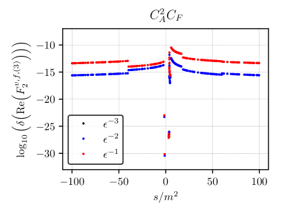
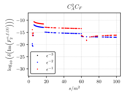
(a)	(b)
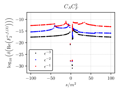
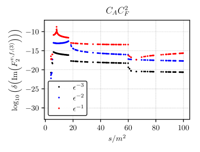
(c)	(d)
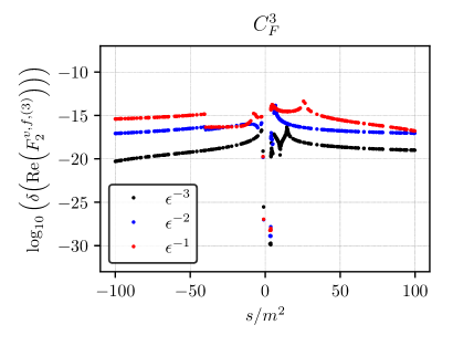
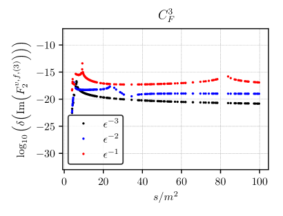
(e)	(f)

Figure 11: Relative cancellation of the real, (a), (c), (e), and imaginary parts, (b), (d), (f), of the poles for the non-fermionic colour structures of $F^{v,f,(3)}_{2}$, c.f. Eq. (31). Note that the $1/\epsilon^{3}$ pole of the colour factor $C_{A}^{2}C_{F}$ is zero.

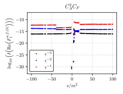
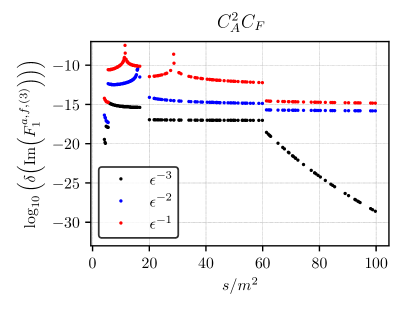
(a)	(b)
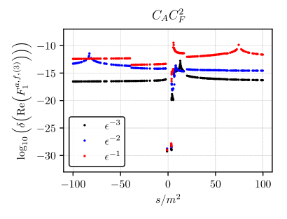
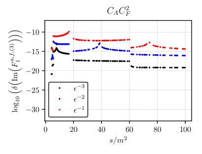
(c)	(d)
(e)	(f)

Figure 12: Relative cancellation of the real, (a), (c), (e), and imaginary parts, (b), (d), (f), of the poles for the non-fermionic colour structures of $F^{a,f,(3)}_{1}$, c.f. Eq. (31).

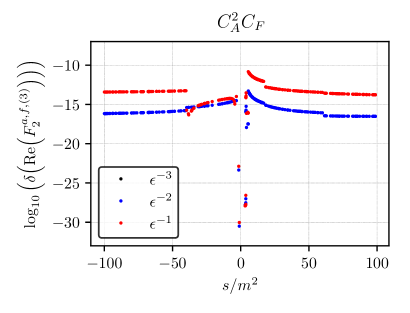
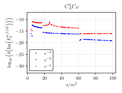
(a)	(b)
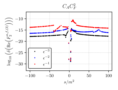
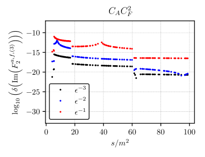
(c)	(d)
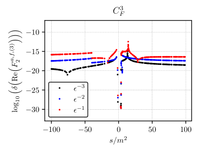
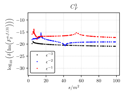
(e)	(f)

Figure 13: Relative cancellation of the real, (a), (c), (e), and imaginary parts, (b), (d), (f), of the poles for the non-fermionic colour structures of $F^{a,f,(3)}_{2}$, c.f. Eq. (31). Note that the $1/\epsilon^{3}$ pole of the colour factor $C_{A}^{2}C_{F}$ is zero.

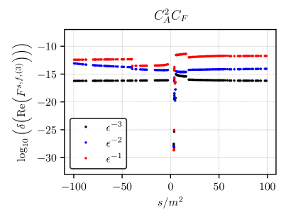
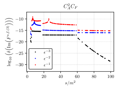
(a)	(b)
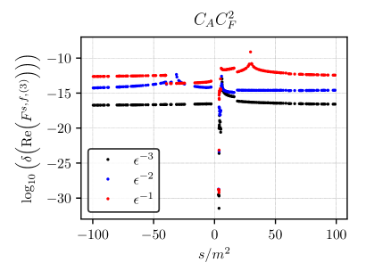
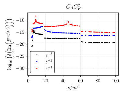
(c)	(d)
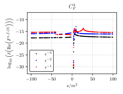
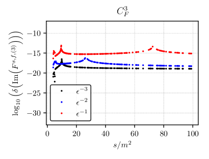
(e)	(f)

Figure 14: Relative cancellation of the real, (a), (c), (e), and imaginary parts, (b), (d), (f), of the poles for the non-fermionic colour structures of $F^{s,f,(3)}$, c.f. Eq. (31).

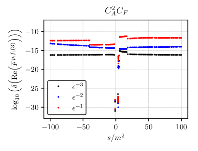
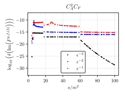
(a)	(b)
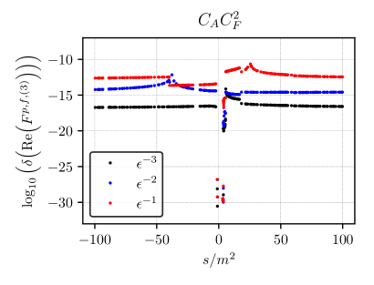
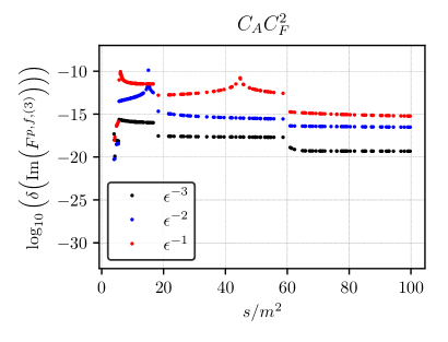
(c)	(d)
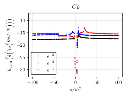
(e)	(f)

Figure 15: Relative cancellation of the real, (a), (c), (e), and imaginary parts, (b), (d), (f), of the poles for the non-fermionic colour structures of $F^{p,f,(3)}$, c.f. Eq. (31).

Appendix C Analytic results for $s\to 0$

In the following we present analytic expansion $s\to 0$ of three-loop term for the non-singlet form factors $F_{2}^{v}$, $F_{1}^{a}$, $F_{2}^{a}$ and $F^{p}$. The results for $F_{1}^{v}$ and $F^{s}$ can be found in Section 6.2.1. Our results read

$$F_{2}^{v,f,(3)}\Big{|}_{s\to 0}=C_{A}C_{F}^{2}\Bigg{[}-\frac{20a_{4}}{3}-\frac{113\zeta_{3}}{48}-\frac{5\pi^{2}\zeta_{3}}{12}+\frac{185\zeta_{5}}{24}-\frac{955}{72}+\frac{1505\pi^{2}}{432}-\frac{35\pi^{4}}{432}-\frac{5l_{2}^{4}}{18}$$

$$\quad+\frac{49}{36}\pi^{2}l_{2}^{2}-\frac{31}{12}\pi^{2}l_{2}\Bigg{]}+C_{A}^{2}C_{F}\Bigg{[}\frac{5a_{4}}{3}-\frac{\zeta_{3}}{2}+\frac{29\pi^{2}\zeta_{3}}{288}-\frac{65\zeta_{5}}{32}+\frac{31231}{2592}-\frac{463\pi^{2}}{216}+\frac{103\pi^{4}}{2880}$$

$$\quad+\frac{5l_{2}^{4}}{72}-\frac{11}{18}\pi^{2}l_{2}^{2}+\frac{25}{8}\pi^{2}l_{2}\Bigg{]}+C_{F}^{3}\Bigg{[}\frac{20a_{4}}{3}+\frac{241\zeta_{3}}{24}+\frac{103\pi^{2}\zeta_{3}}{72}-\frac{235\zeta_{5}}{24}-\frac{101}{64}+\frac{23\pi^{2}}{6}$$

$$\quad-\frac{139\pi^{4}}{2160}+\frac{5l_{2}^{4}}{18}-\frac{5}{18}\pi^{2}l_{2}^{2}-\frac{22}{3}\pi^{2}l_{2}\Bigg{]}+C_{F}^{2}T_{F}n_{h}\Bigg{[}\frac{32a_{4}}{3}-\frac{263\zeta_{3}}{72}+\frac{2027}{216}+\frac{11\pi^{2}}{162}+\frac{4\pi^{4}}{135}$$

$$\quad+\frac{4l_{2}^{4}}{9}-\frac{4}{9}\pi^{2}l_{2}^{2}-\frac{16}{9}\pi^{2}l_{2}\Bigg{]}+C_{F}C_{A}T_{F}n_{h}\Bigg{[}-\frac{20a_{4}}{3}-\frac{241\zeta_{3}}{36}+\frac{\pi^{2}\zeta_{3}}{8}-\frac{25\zeta_{5}}{24}+\frac{2099}{162}$$

$$\quad-\frac{1375\pi^{2}}{648}-\frac{143\pi^{4}}{2160}-\frac{5l_{2}^{4}}{18}+\frac{5}{18}\pi^{2}l_{2}^{2}+\frac{32}{9}\pi^{2}l_{2}\Bigg{]}$$

$$\quad+\frac{s}{m^{2}}\Bigg{\{}C_{A}C_{F}^{2}\Bigg{[}-\frac{671a_{4}}{45}-\frac{589907\zeta_{3}}{138240}-\frac{67\pi^{2}\zeta_{3}}{360}+\frac{53\zeta_{5}}{24}-\frac{317}{60}+\frac{967027\pi^{2}}{1088640}+\frac{4867\pi^{4}}{129600}$$

$$\quad-\frac{671l_{2}^{4}}{1080}+\frac{589}{540}\pi^{2}l_{2}^{2}+\frac{49\pi^{2}l_{2}}{2160}\Bigg{]}+C_{A}^{2}C_{F}\Bigg{[}\frac{28a_{4}}{9}-\frac{65\zeta_{3}}{864}-\frac{187\pi^{2}\zeta_{3}}{2880}-\frac{71\zeta_{5}}{192}+\frac{941909}{311040}$$

$$\quad-\frac{9189077\pi^{2}}{10886400}+\frac{\pi^{4}}{1080}+\frac{7l_{2}^{4}}{54}-\frac{823\pi^{2}l_{2}^{2}}{2160}+\frac{649}{480}\pi^{2}l_{2}\Bigg{]}+C_{F}^{3}\Bigg{[}\frac{782a_{4}}{45}+\frac{243809\zeta_{3}}{23040}+\frac{671\pi^{2}\zeta_{3}}{720}$$

$$\quad-\frac{59\zeta_{5}}{16}-\frac{16541}{15360}+\frac{8647501\pi^{2}}{3628800}-\frac{7177\pi^{4}}{64800}+\frac{391l_{2}^{4}}{540}-\frac{71}{108}\pi^{2}l_{2}^{2}-\frac{589}{108}\pi^{2}l_{2}\Bigg{]}$$

$$\quad+C_{F}^{2}T_{F}n_{h}\Bigg{[}\frac{16a_{4}}{3}-\frac{2269\zeta_{3}}{6912}+\frac{811}{405}+\frac{4403\pi^{2}}{77760}+\frac{8\pi^{4}}{675}+\frac{2l_{2}^{4}}{9}-\frac{2}{9}\pi^{2}l_{2}^{2}-\frac{20}{27}\pi^{2}l_{2}\Bigg{]}$$

$$\quad+C_{F}C_{A}T_{F}n_{h}\Bigg{[}-\frac{37a_{4}}{9}-\frac{1493\zeta_{3}}{720}+\frac{\pi^{2}\zeta_{3}}{15}-\frac{\zeta_{5}}{2}+\frac{56369}{9720}-\frac{14623\pi^{2}}{12960}-\frac{3041\pi^{4}}{129600}-\frac{37l_{2}^{4}}{216}$$

$$\quad+\frac{37}{216}\pi^{2}l_{2}^{2}+\frac{221}{135}\pi^{2}l_{2}\Bigg{]}\Bigg{\}}+{\cal O}\left(\frac{s^{2}}{m^{4}}\right)+\mbox{$n_{l}$, $n_{l}^{2}$ and $n_{h}^{2}$ terms},$$ (66)

$$F_{1}^{a,f,(3)}\Big{|}_{s\to 0}=C_{A}C_{F}^{2}\Bigg{[}\frac{52a_{4}}{9}-\frac{79\zeta_{3}}{24}+\frac{\pi^{2}\zeta_{3}}{18}+\frac{65\zeta_{5}}{12}-\frac{2723}{864}+\frac{467\pi^{2}}{288}-\frac{359\pi^{4}}{6480}+\frac{13l_{2}^{4}}{54}$$

$$\quad+\frac{10}{27}\pi^{2}l_{2}^{2}-\frac{215}{108}\pi^{2}l_{2}\Bigg{]}+C_{A}^{2}C_{F}\Bigg{[}-\frac{16a_{4}}{9}+\frac{215\zeta_{3}}{144}+\frac{11\pi^{2}\zeta_{3}}{144}-\frac{5\zeta_{5}}{3}-\frac{16241}{5184}-\frac{1423\pi^{2}}{1728}$$

$$\quad+\frac{97\pi^{4}}{6480}-\frac{2l_{2}^{4}}{27}-\frac{25}{108}\pi^{2}l_{2}^{2}+\frac{139}{108}\pi^{2}l_{2}\Bigg{]}+C_{F}^{3}\Bigg{[}-\frac{40a_{4}}{9}+\frac{40\zeta_{3}}{9}+\frac{7\pi^{2}\zeta_{3}}{12}-\frac{20\zeta_{5}}{3}-\frac{1141}{576}$$

$$\quad+\frac{155\pi^{2}}{216}-\frac{7\pi^{4}}{216}-\frac{5l_{2}^{4}}{27}+\frac{5}{27}\pi^{2}l_{2}^{2}-\frac{7}{6}\pi^{2}l_{2}\Bigg{]}+C_{F}^{2}T_{F}n_{h}\Bigg{[}\frac{32a_{4}}{3}-\frac{355\zeta_{3}}{108}+\frac{202}{81}-\frac{433\pi^{2}}{486}$$

$$\quad+\frac{\pi^{4}}{30}+\frac{4l_{2}^{4}}{9}-\frac{4}{9}\pi^{2}l_{2}^{2}+\frac{16}{27}\pi^{2}l_{2}\Bigg{]}+C_{F}C_{A}T_{F}n_{h}\Bigg{[}-8a_{4}-\frac{121\zeta_{3}}{27}+\frac{7\pi^{2}\zeta_{3}}{36}-\frac{5\zeta_{5}}{4}+\frac{449}{24}$$

$$\quad-\frac{1019\pi^{2}}{243}-\frac{53\pi^{4}}{1080}-\frac{l_{2}^{4}}{3}+\frac{1}{3}\pi^{2}l_{2}^{2}+\frac{136}{27}\pi^{2}l_{2}\Bigg{]}$$

$$\quad+\frac{s}{m^{2}}\Bigg{\{}C_{A}C_{F}^{2}\Bigg{[}\frac{221a_{4}}{50}+\frac{50821\zeta_{3}}{38400}-\frac{41\pi^{2}\zeta_{3}}{180}+\frac{3\zeta_{5}}{32}-\frac{535643}{1036800}-\frac{236713\pi^{2}}{7776000}+\frac{3341\pi^{4}}{259200}$$

$$\quad+\frac{221l_{2}^{4}}{1200}+\frac{41}{300}\pi^{2}l_{2}^{2}+\frac{413\pi^{2}l_{2}}{1800}\Bigg{]}+C_{A}^{2}C_{F}\Bigg{[}-\frac{a_{4}}{18}+\frac{705841\zeta_{3}}{518400}+\frac{7\pi^{2}\zeta_{3}}{120}-\frac{91\zeta_{5}}{192}$$

$$\quad-\frac{13815151}{3499200}+\frac{1480493\pi^{2}}{2332800}+\frac{7\pi^{4}}{259200}-\frac{l_{2}^{4}}{432}+\frac{529\pi^{2}l_{2}^{2}}{4320}-\frac{57931\pi^{2}l_{2}}{43200}\Bigg{]}+C_{F}^{3}\Bigg{[}-\frac{1939a_{4}}{225}$$

$$\quad-\frac{736801\zeta_{3}}{172800}-\frac{7\pi^{2}\zeta_{3}}{60}+\frac{\zeta_{5}}{3}-\frac{1297}{1620}-\frac{386843\pi^{2}}{155520}+\frac{1529\pi^{4}}{25920}-\frac{1939l_{2}^{4}}{5400}-\frac{4121\pi^{2}l_{2}^{2}}{5400}$$

$$\quad+\frac{2119}{432}\pi^{2}l_{2}\Bigg{]}+C_{F}^{2}T_{F}n_{h}\Bigg{[}\frac{16a_{4}}{9}+\frac{413\zeta_{3}}{640}-\frac{1693}{960}+\frac{30919\pi^{2}}{388800}+\frac{29\pi^{4}}{4050}+\frac{2l_{2}^{4}}{27}-\frac{2}{27}\pi^{2}l_{2}^{2}$$

$$\quad-\frac{4}{27}\pi^{2}l_{2}\Bigg{]}+C_{F}C_{A}T_{F}n_{h}\Bigg{[}-\frac{163a_{4}}{90}+\frac{13291\zeta_{3}}{17280}+\frac{23\pi^{2}\zeta_{3}}{720}-\frac{7\zeta_{5}}{48}+\frac{89623}{38880}-\frac{52861\pi^{2}}{77760}$$

$$\quad-\frac{257\pi^{4}}{86400}-\frac{163l_{2}^{4}}{2160}+\frac{163\pi^{2}l_{2}^{2}}{2160}+\frac{323}{540}\pi^{2}l_{2}\Bigg{]}\Bigg{\}}+{\cal O}\left(\frac{s^{2}}{m^{4}}\right)+\mbox{$n_{l}$, $n_{l}^{2}$ and $n_{h}^{2}$ terms},$$ (67)

$$F_{2}^{a,f,(3)}\Big{|}_{s\to 0}=C_{A}C_{F}^{2}\Bigg{[}-\frac{1198a_{4}}{75}+\frac{52189\zeta_{3}}{43200}+\frac{37\pi^{2}\zeta_{3}}{180}-\frac{9\zeta_{5}}{8}-\frac{304243}{129600}+\frac{3289037\pi^{2}}{972000}$$

$$\quad-\frac{1451\pi^{4}}{21600}-\frac{599l_{2}^{4}}{900}+\frac{181}{100}\pi^{2}l_{2}^{2}-\frac{18433\pi^{2}l_{2}}{5400}\Bigg{]}+C_{A}^{2}C_{F}\Bigg{[}\frac{11a_{4}}{3}-\frac{124681\zeta_{3}}{43200}-\frac{161\pi^{2}\zeta_{3}}{480}$$

$$\quad+\frac{27\zeta_{5}}{32}+\frac{2720569}{194400}-\frac{113491\pi^{2}}{64800}+\frac{4753\pi^{4}}{129600}+\frac{11l_{2}^{4}}{72}-\frac{19}{24}\pi^{2}l_{2}^{2}+\frac{8767\pi^{2}l_{2}}{2700}\Bigg{]}+C_{F}^{3}\Bigg{[}\frac{432a_{4}}{25}$$

$$\quad+\frac{211549\zeta_{3}}{21600}+\frac{119\pi^{2}\zeta_{3}}{360}+\frac{3\zeta_{5}}{8}+\frac{61289}{25920}+\frac{43541\pi^{2}}{19440}-\frac{7\pi^{4}}{324}+\frac{18l_{2}^{4}}{25}-\frac{34}{75}\pi^{2}l_{2}^{2}-\frac{1109}{180}\pi^{2}l_{2}\Bigg{]}$$

$$\quad+C_{F}^{2}T_{F}n_{h}\Bigg{[}-\frac{32a_{4}}{9}+\frac{3563\zeta_{3}}{1080}+\frac{12199}{3240}+\frac{13421\pi^{2}}{12150}-\frac{44\pi^{4}}{2025}-\frac{4l_{2}^{4}}{27}+\frac{4}{27}\pi^{2}l_{2}^{2}-\frac{56}{27}\pi^{2}l_{2}\Bigg{]}$$

$$\quad+C_{F}C_{A}T_{F}n_{h}\Bigg{[}\frac{76a_{4}}{15}+\frac{221\zeta_{3}}{2160}-\frac{53\pi^{2}\zeta_{3}}{360}+\frac{17\zeta_{5}}{24}-\frac{14653}{1215}+\frac{34243\pi^{2}}{9720}-\frac{121\pi^{4}}{32400}+\frac{19l_{2}^{4}}{90}$$

$$\quad-\frac{19}{90}\pi^{2}l_{2}^{2}-\frac{464}{135}\pi^{2}l_{2}\Bigg{]}$$

$$\quad+\frac{s}{m^{2}}\Bigg{\{}C_{A}C_{F}^{2}\Bigg{[}-\frac{131288a_{4}}{11025}-\frac{99580907\zeta_{3}}{84672000}+\frac{3\pi^{2}\zeta_{3}}{40}-\frac{55\zeta_{5}}{168}-\frac{106581949}{217728000}$$

$$\quad+\frac{33541132409\pi^{2}}{13335840000}-\frac{101909\pi^{4}}{5292000}-\frac{16411l_{2}^{4}}{33075}+\frac{375539\pi^{2}l_{2}^{2}}{264600}-\frac{8183503\pi^{2}l_{2}}{2646000}\Bigg{]}$$

$$\quad+C_{A}^{2}C_{F}\Bigg{[}\frac{3874a_{4}}{1575}-\frac{32235173\zeta_{3}}{67737600}-\frac{2011\pi^{2}\zeta_{3}}{20160}+\frac{313\zeta_{5}}{1344}+\frac{785687831}{304819200}-\frac{17234629\pi^{2}}{12700800}$$

$$\quad+\frac{11279\pi^{4}}{453600}+\frac{1937l_{2}^{4}}{18900}-\frac{7163\pi^{2}l_{2}^{2}}{10800}+\frac{640589\pi^{2}l_{2}}{294000}\Bigg{]}+C_{F}^{3}\Bigg{[}\frac{51368a_{4}}{3675}+\frac{90221321\zeta_{3}}{12096000}$$

$$\quad+\frac{607\pi^{2}\zeta_{3}}{5040}+\frac{5\zeta_{5}}{112}-\frac{791347117}{1524096000}+\frac{12650994259\pi^{2}}{13335840000}-\frac{35153\pi^{4}}{496125}+\frac{6421l_{2}^{4}}{11025}-\frac{682\pi^{2}l_{2}^{2}}{3675}$$

$$\quad-\frac{478157\pi^{2}l_{2}}{189000}\Bigg{]}+C_{F}^{2}T_{F}n_{h}\Bigg{[}-\frac{16a_{4}}{15}+\frac{310831\zeta_{3}}{1209600}+\frac{1405037}{680400}+\frac{5910619\pi^{2}}{19051200}-\frac{11\pi^{4}}{1575}$$

$$\quad-\frac{2l_{2}^{4}}{45}+\frac{2}{45}\pi^{2}l_{2}^{2}-\frac{28}{45}\pi^{2}l_{2}\Bigg{]}+C_{F}C_{A}T_{F}n_{h}\Bigg{[}\frac{899a_{4}}{525}-\frac{17770021\zeta_{3}}{24192000}-\frac{\pi^{2}\zeta_{3}}{24}+\frac{11\zeta_{5}}{56}$$

$$\quad-\frac{30832783}{15552000}+\frac{23421151\pi^{2}}{34020000}-\frac{3821\pi^{4}}{1512000}+\frac{899l_{2}^{4}}{12600}-\frac{899\pi^{2}l_{2}^{2}}{12600}-\frac{2746\pi^{2}l_{2}}{4725}\Bigg{]}\Bigg{\}}$$

$$\quad+{\cal O}\left(\frac{s^{2}}{m^{4}}\right)+\mbox{$n_{l}$, $n_{l}^{2}$ and $n_{h}^{2}$ terms},$$ (68)

$$F^{p,f,(3)}\Big{|}_{s\to 0}=C_{A}C_{F}^{2}\Bigg{[}\frac{64a_{4}}{9}+\frac{379\zeta_{3}}{96}+\frac{179\pi^{2}\zeta_{3}}{144}+\frac{125\zeta_{5}}{48}-\frac{36869}{13824}+\frac{305\pi^{2}}{576}-\frac{667\pi^{4}}{3240}+\frac{8l_{2}^{4}}{27}$$

$$\quad+\frac{133}{108}\pi^{2}l_{2}^{2}-\frac{55}{54}\pi^{2}l_{2}\Bigg{]}+C_{A}^{2}C_{F}\Bigg{[}-\frac{49a_{4}}{9}-\frac{913\zeta_{3}}{288}-\frac{415\pi^{2}\zeta_{3}}{576}+\frac{35\zeta_{5}}{96}+\frac{932761}{124416}-\frac{33\pi^{2}}{128}$$

$$\quad+\frac{3461\pi^{4}}{51840}-\frac{49l_{2}^{4}}{216}-\frac{29}{54}\pi^{2}l_{2}^{2}+\frac{623}{216}\pi^{2}l_{2}\Bigg{]}+C_{F}^{3}\Bigg{[}\frac{68a_{4}}{9}+\frac{1603\zeta_{3}}{144}+\frac{31\pi^{2}\zeta_{3}}{48}-\frac{175\zeta_{5}}{24}$$

$$\quad+\frac{1957}{1152}+\frac{8143\pi^{2}}{1728}-\frac{5\pi^{4}}{432}+\frac{17l_{2}^{4}}{54}-\frac{17}{54}\pi^{2}l_{2}^{2}-\frac{19}{2}\pi^{2}l_{2}\Bigg{]}+C_{F}^{2}T_{F}n_{h}\Bigg{[}8a_{4}-\frac{233\zeta_{3}}{216}+\frac{6581}{2592}$$

$$\quad-\frac{91\pi^{2}}{486}-\frac{19\pi^{4}}{2160}+\frac{l_{2}^{4}}{3}-\frac{1}{3}\pi^{2}l_{2}^{2}-\frac{8}{27}\pi^{2}l_{2}\Bigg{]}+C_{F}C_{A}T_{F}n_{h}\Bigg{[}-\frac{20a_{4}}{3}-\frac{1609\zeta_{3}}{432}+\frac{5\pi^{2}\zeta_{3}}{72}$$

$$\quad-\frac{5\zeta_{5}}{8}+\frac{142537}{15552}-\frac{4181\pi^{2}}{3888}-\frac{\pi^{4}}{108}-\frac{5l_{2}^{4}}{18}+\frac{5}{18}\pi^{2}l_{2}^{2}+\frac{40}{27}\pi^{2}l_{2}\Bigg{]}$$

$$\quad+\frac{s}{m^{2}}\Bigg{\{}C_{A}C_{F}^{2}\Bigg{[}\frac{32a_{4}}{75}+\frac{653927\zeta_{3}}{345600}-\frac{127\pi^{2}\zeta_{3}}{720}-\frac{3\zeta_{5}}{16}-\frac{383557}{518400}+\frac{2078087\pi^{2}}{2592000}-\frac{253\pi^{4}}{64800}$$

$$\quad+\frac{4l_{2}^{4}}{225}+\frac{707\pi^{2}l_{2}^{2}}{1200}-\frac{14917\pi^{2}l_{2}}{21600}\Bigg{]}+C_{A}^{2}C_{F}\Bigg{[}\frac{31a_{4}}{36}+\frac{165899\zeta_{3}}{259200}-\frac{49\pi^{2}\zeta_{3}}{1920}-\frac{101\zeta_{5}}{384}$$

$$\quad-\frac{3145181}{6998400}+\frac{229537\pi^{2}}{1166400}+\frac{1589\pi^{4}}{172800}+\frac{31l_{2}^{4}}{864}-\frac{163\pi^{2}l_{2}^{2}}{2160}-\frac{7621\pi^{2}l_{2}}{14400}\Bigg{]}+C_{F}^{3}\Bigg{[}-\frac{967a_{4}}{225}$$

$$\quad-\frac{348263\zeta_{3}}{172800}-\frac{49\pi^{2}\zeta_{3}}{1440}+\frac{41\zeta_{5}}{96}-\frac{122719}{207360}-\frac{289267\pi^{2}}{155520}+\frac{463\pi^{4}}{8640}-\frac{967l_{2}^{4}}{5400}-\frac{4733\pi^{2}l_{2}^{2}}{5400}$$

$$\quad+\frac{1889}{540}\pi^{2}l_{2}\Bigg{]}+C_{F}^{2}T_{F}n_{h}\Bigg{[}\frac{8a_{4}}{9}+\frac{25403\zeta_{3}}{17280}-\frac{13927}{17280}+\frac{140537\pi^{2}}{388800}+\frac{7\pi^{4}}{4050}+\frac{l_{2}^{4}}{27}-\frac{1}{27}\pi^{2}l_{2}^{2}$$

$$\quad-\frac{2}{3}\pi^{2}l_{2}\Bigg{]}+C_{F}C_{A}T_{F}n_{h}\Bigg{[}-\frac{49a_{4}}{90}+\frac{13733\zeta_{3}}{17280}-\frac{7\pi^{2}\zeta_{3}}{1440}+\frac{\zeta_{5}}{32}-\frac{27601}{38880}+\frac{3125\pi^{2}}{15552}$$

$$\quad-\frac{1013\pi^{4}}{259200}-\frac{49l_{2}^{4}}{2160}+\frac{49\pi^{2}l_{2}^{2}}{2160}-\frac{47}{180}\pi^{2}l_{2}\Bigg{]}\Bigg{\}}+{\cal O}\left(\frac{s^{2}}{m^{4}}\right)+\mbox{$n_{l}$, $n_{l}^{2}$ and $n_{h}^{2}$ terms},$$ (69)

For the vector and pseudo-scalar singlet form factor we have

$$F_{1,\,\text{sing}}^{v,f,(3)}\Big{|}_{s\to 0}={-\frac{s}{m^{2}}}\Bigg{\{}\frac{(d^{abc})^{2}n_{h}}{N_{c}}\Bigg{[}\frac{50a_{4}}{9}-\frac{143\zeta_{3}}{216}+\frac{337}{1296}+\frac{43841\pi^{2}}{4860}-\frac{107\pi^{4}}{2592}+\frac{25l_{2}^{4}}{108}-$$

$$\quad\frac{25}{108}\pi^{2}l_{2}^{2}-\frac{341}{27}\pi^{2}l_{2}\Bigg{]}\Bigg{\}}+{\cal O}\left(\frac{\sqrt{-s}^{4}}{m^{4}}\right)\,,$$ (70)

$$F_{2,\,\text{sing}}^{v,f,(3)}\Big{|}_{s\to 0}=\frac{(d^{abc})^{2}n_{h}}{N_{c}}\Bigg{[}16a_{4}-\frac{4\zeta_{3}}{3}-\frac{5\pi^{2}\zeta_{3}}{18}+\frac{5\zeta_{5}}{6}+\frac{5}{9}+\frac{931\pi^{2}}{54}-\frac{41\pi^{4}}{540}+\frac{2l_{2}^{4}}{3}-\frac{2}{3}\pi^{2}l_{2}^{2}$$

$$\quad-24\pi^{2}l_{2}\Bigg{]}$$

$$\quad{-\frac{s^{2}}{m^{2}}}\Bigg{\{}\frac{(d^{abc})^{2}n_{h}}{N_{c}}\Bigg{[}-\frac{116a_{4}}{9}-\frac{887\zeta_{3}}{360}+\frac{\pi^{2}\zeta_{3}}{36}-\frac{\zeta_{5}}{12}+\frac{86}{135}-\frac{234329\pi^{2}}{18900}+\frac{2707\pi^{4}}{32400}$$

$$\quad-\frac{29l_{2}^{4}}{54}+\frac{29}{54}\pi^{2}l_{2}^{2}+\frac{793}{45}\pi^{2}l_{2}\Bigg{]}\Bigg{\}}+{\cal O}\left(\frac{\sqrt{-s}^{4}}{m^{4}}\right)\,,$$ (71)

$$F_{\text{sing}}^{p,f,(3)}\Big{|}_{s\to 0}=C_{A}C_{F}T_{F}n_{h}\Bigg{[}8a_{4}+\frac{103\zeta_{3}}{24}+\frac{1133}{864}+\frac{3401\pi^{2}}{2592}+\frac{2\pi^{4}}{135}+\frac{l_{2}^{4}}{3}-\frac{1}{3}\pi^{2}l_{2}^{2}-2\pi^{2}l_{2}\Bigg{]}$$

$$\quad+C_{F}^{2}T_{F}n_{h}\Bigg{[}-8a_{4}-\frac{71\zeta_{3}}{36}+\frac{37}{216}+\frac{1195\pi^{2}}{648}-\frac{\pi^{4}}{40}-\frac{l_{2}^{4}}{3}+\frac{1}{3}\pi^{2}l_{2}^{2}-\frac{4}{3}\pi^{2}l_{2}\Bigg{]}$$

$$\quad+C_{F}T_{F}^{2}n_{h}^{2}\Bigg{[}-\frac{16\zeta_{3}}{9}-\frac{1}{27}+\frac{26\pi^{2}}{81}\Bigg{]}+C_{F}T_{F}^{2}n_{h}n_{l}\Bigg{[}-\frac{11}{27}-\frac{17\pi^{2}}{81}\Bigg{]}$$

$$\quad+\frac{\sqrt{-s}}{m}\Bigg{\{}C_{A}C_{F}T_{F}n_{h}\Bigg{[}\frac{19}{48}\pi^{2}l_{\sqrt{-s}/m}+\frac{\pi^{4}}{48}-\frac{565\pi^{2}}{576}\Bigg{]}+C_{F}^{2}T_{F}n_{h}\Bigg{[}-\frac{5\pi^{2}}{16}\Bigg{]}$$

$$\quad+C_{F}T_{F}^{2}n_{h}n_{l}\Bigg{[}\frac{19\pi^{2}}{72}-\frac{1}{6}\pi^{2}l_{\sqrt{-s}/m}\Bigg{]}\Bigg{\}}$$

$$\quad{-\frac{s}{m^{2}}}\Bigg{\{}C_{A}C_{F}T_{F}n_{h}\Bigg{[}-\frac{67a_{4}}{90}+\frac{11l_{\sqrt{-s}/m}^{2}}{24}+\frac{1}{15}\pi^{2}l_{\sqrt{-s}/m}-\frac{287l_{\sqrt{-s}/m}}{144}-\frac{20977\zeta_{3}}{43200}$$

$$\quad-\frac{1139\pi^{4}}{259200}-\frac{10358353\pi^{2}}{27216000}+\frac{1843381}{1036800}-\frac{67l_{2}^{4}}{2160}+\frac{67\pi^{2}l_{2}^{2}}{2160}+\frac{547\pi^{2}l_{2}}{1350}\Bigg{]}+C_{F}^{2}T_{F}n_{h}\Bigg{[}\frac{6a_{4}}{5}$$

$$\quad-\frac{l_{\sqrt{-s}/m}}{2}+\frac{1463\zeta_{3}}{57600}+\frac{17\pi^{4}}{4320}+\frac{56269\pi^{2}}{362880}+\frac{296969}{345600}+\frac{l_{2}^{4}}{20}-\frac{1}{20}\pi^{2}l_{2}^{2}-\frac{52}{135}\pi^{2}l_{2}\Bigg{]}$$

$$\quad+C_{F}T_{F}^{2}n_{h}^{2}\Bigg{[}\frac{97\zeta_{3}}{216}+\frac{13}{648}-\frac{394\pi^{2}}{6075}\Bigg{]}+C_{F}T_{F}^{2}n_{h}n_{l}\Bigg{[}-\frac{1}{6}l_{\sqrt{-s}/m}^{2}+\frac{19l_{\sqrt{-s}/m}}{36}+\frac{263\pi^{2}}{4860}$$

$$\quad-\frac{353}{1296}\Bigg{]}\Bigg{\}}+{\cal O}\left(\frac{\sqrt{-s}^{3}}{m^{3}}\right)\,$$ (72)

The result for $F_{\rm sing}^{s,f,(3)}$ is given in Eq. (34).