Reliable Representations Make A Stronger Defender: Unsupervised Structure Refinement for Robust GNN

Abstract.

Benefiting from the message passing mechanism, Graph Neural Networks (GNNs) have been successful on flourish tasks over graph data. However, recent studies have shown that attackers can catastrophically degrade the performance of GNNs by maliciously modifying the graph structure. A straightforward solution to remedy this issue is to model the edge weights by learning a metric function between pairwise representations of two end nodes, which attempts to assign low weights to adversarial edges. The existing methods use either raw features or representations learned by supervised GNNs to model the edge weights. However, both strategies are faced with some immediate problems: raw features cannot represent various properties of nodes (e.g., structure information), and representations learned by supervised GNN may suffer from the poor performance of the classifier on the poisoned graph. We need representations that carry both feature information and as mush correct structure information as possible and are insensitive to structural perturbations. To this end, we propose an unsupervised pipeline, named STABLE, to optimize the graph structure. Finally, we input the well-refined graph into a downstream classifier. For this part, we design an advanced GCN that significantly enhances the robustness of vanilla GCN (Kipf and Welling, 2017) without increasing the time complexity. Extensive experiments on four real-world graph benchmarks demonstrate that STABLE outperforms the state-of-the-art methods and successfully defends against various attacks. The implementation of STABLE is available at https://github.com/likuanppd/STABLE

1. Introduction

Graphs are ubiquitous data structures that can represent various objects and their complex relations (Zhang et al., 2020; Battaglia et al., 2018; Zhou et al., 2020; Liu et al., 2021a; Zhu et al., 2021a). As a powerful tool of learning representations from graphs, Graph Neural Networks (GNNs) burgeon widely explorations in recent years (Li et al., 2016; Kipf and Welling, 2017; Hamilton et al., 2017; Veličković et al., 2017; Xu et al., 2019b) for numerous graph-based tasks, primarily focused on node representation learning (Perozzi et al., 2014; Kipf and Welling, 2016; Veličković et al., 2018; You et al., 2020) and transductive node classification (Kipf and Welling, 2017; Hamilton et al., 2017; Veličković et al., 2017; Huang et al., 2022). The key to the success of GNNs is the neural message passing mechanism, in which GNNs regard features and hidden representations as messages carried by nodes and propagate them through the edges. However, this mechanism also brings a security risk.

Table 1. The mean accuracy under different perturbation rates by MetaAttack on the Cora dataset. Here the perturbation rate is the ratio of changed edges. The data split follows 10%/ 10%/ 80/%(train/ validation/ test).

Ptb Rate	GCN	GRCN	GNNGuard	Jaccard
0%	83.56	86.12	78.52	81.79
5%	76.36	80.78	77.96	80.23
10%	71.62	72.42	74.86	74.65
20%	60.31	65.43	72.03	73.11

Recent studies have shown that GNNs are vulnerable to adversarial attacks (Dai et al., 2018; Zügner et al., 2018; Zügner and Günnemann, 2019; Wu et al., 2019; Zhu et al., 2022). In other words, by limitedly rewiring the graph structure or just perturbing a small part of the node features, attackers can easily fool the GNNs to misclassify nodes in the graph. The robustness of the model is essential for some security-critical domains. For instance, in fraudulent transaction detection, fraudsters can conceal themselves by deliberately dealing with common users. Thus, it is necessary to study the robustness of GNNs. Although attackers can modify the clean graph by perturbing node features or the graph structure, most of the existing adversarial attacks on graph data have concentrated on modifying graph structure (Zügner and Günnemann, 2019; Finkelshtein et al., 2020). Moreover, the structure perturbation is considered more effective (Zügner et al., 2018; Wu et al., 2019) probably due to the message passing mechanism. Misleading messages will pass through a newly added edge, or correct messages cannot be propagated because an original edge is deleted. In this paper, our purpose is to defend against the non-targeted adversarial attack on graph data that attempts to reduce the overall performance of the GNN. Under this setting, the GNNs are supposed to be trained on a graph that the structure has already been perturbed.

One representative perspective to defend against the attack is to refine the graph structure by reweighting the edges (Zhu et al., 2021b). Specifically, edge weights are derived from learning a metric function between pairwise representations (Zhang and Zitnik, 2020; Wang et al., 2020; Li et al., 2018; Veličković et al., 2017; Fatemi et al., 2021). Intuitively, the weight of an edge could be represented as a distance measure between two end nodes, and defenders can further prune or add edges according to such distances.

Though extensive approaches have been proposed to model the pairwise weights, most research efforts are devoted to designing a novel metric function, while the rationality of the inputs of the function is inadequately discussed. In more detail, they usually utilize the original features or representations learned by the supervised GNNs to compute the weights.

However, optimizing graph structures based on either features or supervised signals might not be reliable. For example, GNNGuard (Zhang and Zitnik, 2020) and Jaccard(Wu et al., 2019) utilize cosine similarity of the initial features to model the edge weights, while GRCN (Yu et al., 2020) uses the inner product of learned representations. The performance of these three models on Cora attacked by MetaAttack (Zügner and Günnemann, 2019) is listed in Table 1. From the table, we first observe feature-based methods do not perform well under low perturbation rates, because features cannot carry structural information. Optimizing the structure based on such an insufficient property can lead to mistakenly deleting normal edges (the statistics of the removed edges is listed in Table 3). When the perturbation is low, the negative impact of such mis-deletion is greater than the positive impact of deleting malicious edges.Thus, we want to refine the structure by learned representations which contain structural information. Second, we also see the representations learned by the supervised GNNs are not reliable under high perturbations (the results of GRCN). This is probably because attack methods are designed to degrade the accuracy of a surrogate GNN, so the quality of representations learned by the classifier co-vary with the task performance.

Based on the above analysis, we consider that the representations used for structure refining should be obtained in a different manner, and two factors in terms of learning representations in the adversarial scenario should be highlighted: 1) carrying feature information and in the meantime carrying as much correct structure information as possible and 2) insensitivity to structural perturbations.

To this end, we propose an approach named STABLE (STructure leArning GNN via more reliaBLe rEpresentations) in this paper, and it learns the representations used for structure refining by unsupervised learning. The unsupervised approach is relatively reliable because the objective is not directly attacked. Additionally, the unsupervised pipeline can be viewed as a kind of pretraining, and the learned representations may have been trained to be invariant to certain useful properties (Wiles et al., 2022) (i.e., the perturbed structure here). We design a contrastive method with a novel pre-process and recovery schema to obtain the representations. Different from the previous contrastive method (Veličković et al., 2018; Hassani and Khasahmadi, 2020; Peng et al., 2020; Zhu et al., 2020), we roughly refine the graph to remove the easily detectable adversarial edges and generate augmentation views by randomly recovering a small portion of removed edges. Pre-processing makes the underlying structural information obtained during the representation learning process relatively correct, and such an augmentation strategy can be viewed as injecting slight attack to the pre-processed graph. Then the representations learned on different augmentation views tend to be similar during the contrastive training. That is to say, we obtain representations insensitive to the various slight attacks. Such learned representations fulfill our requirements and can be utilized to perform graph structure refinement to derive an unpolluted graph.

In addition, any GNNs can be used for the downstream learning tasks after the structure is well-refined. For this part, many methods (Jin et al., 2020b, 2021) just use the vanilla GCN (Kipf and Welling, 2017). By observing what makes edge insertion or deletion a strong adversarial change, we find that GCN falls victim to its renormalization trick. Hence we introduce an advanced message passing in the GCN module to further improve the robustness.

Our contributions can be summarized as follow:

(1) We propose a contrastive method with robustness-oriented augmentations to obtain the representations used for structure refining, which can effectively capture structural information of nodes and are insensitive to the perturbations. (2) We further explore the reason for the lack of robustness of GCN and propose a more robust normalization trick. (3) Extensive experiments on four real-world datasets demonstrate that STABLE can defend against different types of adversarial attacks and outperform the state-of-the-art defense models.

2. Preliminaries

2.1. Graph Neural Networks

Let $\mathcal{G}=\{\mathcal{V},\mathcal{E},\mathbf{X}\}$ represent a graph with $N$ nodes, where $\mathcal{V}$ is the node set, $\mathcal{E}$ is the edge set, and $\mathbf{X}\in\mathbb{R}^{N\times d}$ is the original feature matrix of nodes. Let $\mathbf{A}\in\{0,1\}^{N\times N}$ represent the adjacency matrix of $\mathcal{G}$, in which $\mathbf{A}_{ij}\in\{0,1\}$ denotes the existence of the edge $e_{ij}\in\mathcal{E}$ that links node $v_{i}$ and $v_{j}$. The first-order neighborhood of node $v_{i}$ is denoted as $\mathcal{N}_{i}$, including node $v_{i}$ itself. We use $\mathcal{N}_{i}^{*}$ to indicate $v_{i}$’s neighborhood excluding itself. The transductive node classification task can be formulated as we now describe. Given a graph $\mathcal{G}$ and a subset $\mathcal{V}_{L}\subseteq\mathcal{V}$ of labeled nodes, with class labels from $\mathcal{C}=\{c_{1},c_{2},...,c_{K}\}$. $\mathcal{Y}_{L}$ and $\mathcal{Y}_{U}$ denote the ground-truth labels of labeled nodes and unlabeled nodes, respectively. The goal is to train a GNN $f_{\theta}$ to learn a function: $\mathcal{V}\rightarrow\mathcal{Y}$ that maps the nodes to the label set so that $f_{\theta}$ can predict labels of unlabeled nodes. $\theta$ is the trainable parameters of GNN.

GNNs can be generally specified as $f_{\theta}(\mathbf{X},\mathbf{A})$ (Zhou et al., 2020; Kipf and Welling, 2017; Hamilton et al., 2017). Each layer can be divided into a message passing function (MSP) and an updating function (UPD). Given a node $v_{i}$ and its neighborhood $\mathcal{N}_{i}^{*}$, GNN first implements MSP to aggregate information from $\mathcal{N}_{i}^{*}$: $\bm{m}_{i}^{t}=\textrm{MSP}(\{\bm{h}_{j}^{t-1};j\in\mathcal{N}_{i}^{*}\})$, where $\bm{h}_{j}^{t-1}$ denotes the hidden representation in the previous layer, and $\bm{h}_{j}^{0}=\bm{x}_{j}$. Then, GNN updates the representation by UPD: $\bm{h}_{i}^{t}=\textrm{UPD}(\bm{m}_{i}^{t},\bm{h}_{i}^{t-1})$, which is usually a sum or concat function. GNNs can be designed in an end-to-end fashion and can also serve as a representation learner for downstream tasks (Kipf and Welling, 2017).

2.2. Gray-box Poisoning Attacks and Defence

In this paper, we explore the robustness of GNNs under non-targeted Gray-box poisoning attack. Gray-box (Yu et al., 2020) means the attacker holds the same data information as the defender, and the defense model is unknown. Poisoning attack represents GNNs are trained on a graph that attackers maliciously modify, and the aim of it is to find an optimal perturbed $\mathbf{A}^{\prime}$, which can be formulated as a bilevel optimization problem (Zügner et al., 2018; Zügner and Günnemann, 2019):

(1) $$\begin{split}\underset{A^{\prime}\in\Phi(A)}{\textrm{argmin}}\quad\mathcal{L}_{atk}(f_{\theta^{*}}(\mathbf{A}^{\prime},\mathbf{X}))\quad\\ s.t.\quad\theta^{*}=\underset{\theta}{\textrm{argmin}}\ \mathcal{L}_{train}(f_{\theta}(\mathbf{A}^{\prime},\mathbf{X})).\end{split}$$

Here $\Phi(\mathbf{A})$ is a set of adjacency matrix that fit the constraint: $\frac{\left\|\mathbf{A}^{\prime}-\mathbf{A}\right\|_{0}}{\left\|\mathbf{A}\right\|_{0}}\leq\Delta$, $\mathcal{L}_{atk}$ is the attack loss function, and $\mathcal{L}_{train}$ is the training loss of GNN. The $\theta^{*}$ is the optimal parameter for $f_{\theta}$ on the perturbed graph. $\Delta$ is the maximum perturbation rate. In the non-targeted attack setting, the attacker aims to degrade the overall performance of the classifier.

Many efforts have been made to improve the robustness of GNNs  (Xu et al., 2019a; Zhu et al., 2019; Entezari et al., 2020; Jin et al., 2020b; Liu et al., 2021b; Jin et al., 2021). Among them, metric learning approach (Zhu et al., 2021b) is a promising method (Li et al., 2018; Zhang and Zitnik, 2020; Wang et al., 2020; Chen et al., 2020b), which refines the graph structure by learning a pairwise metric function $\phi(\cdot,\cdot)$:

(2) $$\textbf{S}_{ij}=\phi(\bm{z}_{i},\bm{z}_{j}),$$

where $\bm{z}_{i}$ is the raw feature or the learned embedding of node $v_{i}$ produced by GNN, and $\textbf{S}_{ij}$ denotes the learned edge weight between node $v_{i}$ and $v_{j}$. $\phi(\cdot,\cdot)$ can be a similarity metric or implemented in multilayer perceptions (MLPs). Further, the structure can be optimized according to the weights matrix $\mathbf{S}$. For example, GNNGuard (Zhang and Zitnik, 2020) utilizes cosine similarity to model the edge weights and then calculates edge pruning probability through a non-linear transformation. Moreover, GRCN (Yu et al., 2020) and GAUGM (Zhao et al., 2021) directly compute the weights of the edges by the inner product of embeddings, and no additional parameters are needed:

(3) $$\textbf{S}_{ij}=\sigma(\mathbf{ZZ}^{\mathrm{T}}).$$

Such methods aim to assign high weights to helpful edges and low weights to adversarial edges or even remove them. Here we want to define what is a helpful edge. Existing literature posits that strong homophily of the underlying graph is necessary for GNNs to achieve good performance on transductive node classification (Abu-El-Haija et al., 2019; Chien et al., 2021; Hou et al., 2019). Under the homophily assumption (McPherson et al., 2001), the edge which links two similar nodes (e.g., same label) might help the nodes to be correctly classified. However, since only few labeled nodes are available, previous works utilize the raw features or the representations learned by the task-relevant GNNs to search for similar nodes.

Different from the aforementioned defense methods, we leverage an unsupervised pipeline to calculate the weights matrix and refine the graph structure.

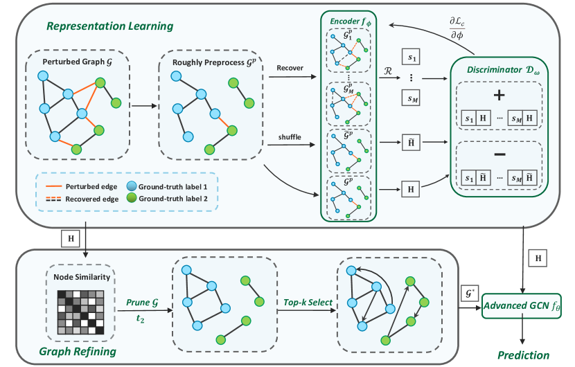
Figure 1. Overall framework. Dash lines mean recovered edges.

3. Method

In this section, we will present STABLE in a top-down fashion: starting with an elaboration of the overall framework, followed by the specific details of the structural optimization module, and concluding by an exposition of the advanced GCN.

3.1. The Overall Architecture

The illustration of the framework is shown in Fig. 1. It consists of two major components, the structure learning network and the advanced GCN classifier. The structure learning network can be further divided into two parts, representation learning and graph refining. For the representation learning part, we design a novel contrastive learning method with a robustness-oriented graph data augmentation, which randomly recovers the roughly removed edges. Then the learned representations are utilized to revise the structure according to the homophily assumption (McPherson et al., 2001). Finally, in the classification step, by observing what properties the nodes connected by the adversarial edges have, we carefully change the renormalization trick in GCN(Kipf and Welling, 2017) to improve the robustness. The overall training algorithm is shown in Appendix A.1.

3.2. Representation learning

According to (Zügner and Günnemann, 2019; Wu et al., 2019), most of the perturbations are edge insertions, which connect nodes with different labels. Thus a straightforward method to deal with the structural perturbation is to find the adversarial edges and remove them. Previous works utilize the raw features or the representations learned by the end-to-end GNNs to seek the potential perturbations. As we mentioned before, such approaches have flaws.

STABLE avoids the pitfalls by leveraging a task-irrelevant contrastive method with robustness-oriented augmentations to learn the representations. First, we roughly pre-process the perturbed graph based on a similarity measure, e.g., Jaccard similarity or cosine similarity. We quantify the score $\textbf{S}_{ij}$ between node $v_{i}$ and its neighbor $v_{j}$ as follows:

(4) $$\textbf{S}_{ij}=\textrm{sim}(\bm{x}_{i},\bm{x}_{j}),$$

where $\mathcal{S}$ is the score matrix, $\bm{x}_{i}$ and $\bm{x}_{j}$ are the feature vectors of $v_{i}$ and $v_{j}$, respectively. Then we prune the edges whose scores are below a threshold $t_{1}$. The removed edge matrix and roughly pre-processed graph are denoted as E and $\mathcal{G}^{P}$, where $\textbf{E}_{ij}=1$ denotes the edge between $v_{i}$ and $v_{j}$ is removed.

Generating views is the key component of contrastive methods. Different views of a graph provide different contexts for each node, and we hope our views carry the context for enhancing the robustness of the representations. Previous works generate augmentations by randomly perturbing the structure (Zhu et al., 2020; You et al., 2020) on the initial graph. Different from them, we generate $M$ graph views, denoted as $\mathcal{G}_{1}^{P}$ to $\mathcal{G}_{M}^{P}$, by randomly recovering a small portion of E on the pre-processed graph $\mathcal{G}^{P}$. Formally, we first sample a random masking matrix $\textbf{P}\in\{0,1\}^{N\times N}$, whose entry is drawn from a Bernoulli distribution $\textbf{P}_{ij}\sim\mathcal{B}(1-p)$ if $\textbf{E}_{ij}=1$ and $\textbf{P}_{ij}=0$ otherwise. Here $p$ is a hyper-parameter that controls the recovery ratio. The adjacency matrix of the augmentation view can be computed as:

(5) $$\mathbf{A}_{1}^{P}=\mathbf{A}^{P}+\textbf{E}\odot\textbf{P},$$

where $\mathbf{A}^{P}$ and $\mathbf{A}_{1}^{P}$ denote the adjacency matrix of $\mathcal{G}^{P}$ and $\mathcal{G}_{1}^{P}$ respectively, and $\odot$ is the Hadamard product. Other views can be obtained in the same way. The pre-process and the robustness-oriented augmentations are critical to the robustness, and we will elaborate on this point at the end of this subsection.

Our objective is to learn a one-layer GCN encoder $f_{\phi}$ parameterized by $\phi$ to maximize the mutual information between the local representation in $\mathcal{G}^{P}$ and the global representations in $\mathcal{G}_{j}$. Here $\mathcal{G}_{j}$ denote arbitrary augmentation $j$. The encoder follows the propagation rule:

(6) $$f_{\phi}(\mathbf{X},\mathbf{A})=\sigma(\hat{\mathbf{A}}\mathbf{X}\textbf{W}_{\phi})$$

where $\hat{\mathbf{A}}=(\textbf{D}+\textbf{I}_{N})^{-\frac{1}{2}}(\mathbf{A}+\textbf{I}_{N})(\textbf{D}+\textbf{I}_{N})^{-\frac{1}{2}}$ is the renormalized adjacency matrix. we denote node representations in $\mathcal{G}^{P}$ and augmentation $j$ as $\textbf{H}=f_{\phi}(\mathbf{X},\mathbf{A}^{P})$ and $\textbf{H}_{j}=f_{\phi}(\mathbf{X},\mathbf{A}_{j}^{P})$. The global representation can be obtained via a readout function $\mathcal{R}$. We leverage a global average pooling function:

(7) $$\bm{s}_{j}=\sigma\left(\frac{1}{N}\sum_{i=1}^{N}\bm{h}_{i,j}\right),$$

where $\sigma$ is the logistic sigmoid nonlinearity, and $\bm{h}_{i,j}$ is the representation of node $v_{i}$ in $\mathcal{G}_{j}^{P}$. We employ a discriminator $\mathcal{D}_{\omega}$ to distinguish positive samples and negative samples, and the output $\mathcal{D}_{\omega}(\bm{h},\bm{s})$ represents the probability score of the sample pair from the joint distribution. $\omega$ is the parameters of the discriminator. To generate negative samples, which means the pair sampled from the product of marginals, we randomly shuffle the nodes’ features in $\mathcal{G}^{P}$. We denote the shuffled graph and its representation as $\widetilde{\mathcal{G}}^{P}$ and $\widetilde{\textbf{H}}=f_{\phi}(\widetilde{\mathbf{X}},\mathbf{A}^{P})$. To maximize the mutual information, we use a binary cross-entropy loss between the positive samples and negative samples, and the objective can be writen as:

(8) $$\begin{split}\mathcal{L}_{C}=-\frac{1}{2N}\sum_{i=1}^{N}\Biggl{(}\frac{1}{M}\sum_{j=1}^{M}\biggl{(}\textrm{log}\mathcal{D}_{\omega}(\bm{h}_{i},\bm{s}_{j})+\textrm{log}\Bigl{(}1-\mathcal{D}_{\omega}(\tilde{\bm{h}}_{i},\bm{s}_{j})\Bigr{)}\biggr{)}\Biggr{)}.\end{split}$$

where $\bm{h}_{i}$ and $\tilde{\bm{h}}_{i}$ are the representations of node $v_{i}$ in $\mathcal{G}^{P}$ and $\widetilde{\mathcal{G}}^{P}$. Minimizing this objective function can effectively maximize the mutual information between the local representations in $\mathcal{G}^{P}$ and the global representations in the augmentations based on the Jensen-Shannon MI (mutual information) estimator(Hjelm et al., 2019).

To clarify why pre-processing and the designed augmentation method are crucial to robustness, we count the results of the pre-process and the recovery: Using Jaccard as the measure of the rough pre-process, $1,705$ edges are removed on Cora under 20% perturbation rate. Among them, 691 are adversarial edges, and 1014 are normal edges. 259 edges out of $1,014$ connect two nodes with different labels. More than half of the removals are helpful. Therefore, most of the edges in E can be regarded as adversarial edges so that the recovery can be viewed as injecting slight attacks on $\mathcal{G}^{P}$. The degrees of perturbation can be ranked as $\mathcal{G}\gg\mathcal{G}_{1}^{P}\approx\mathcal{G}_{2}^{P}\ ...\approx\mathcal{G}_{M}^{P}>\mathcal{G}^{P}$.

Recall that we need representations that carry as much correct structural information as possible and are insensitive to perturbations. We train our encoder on the much cleaner graphs, i.e., $\mathcal{G}^{P}$ and the views, so the representations are much better than those learned in the original graph. The process of maximizing mutual information makes the representations learned in $\mathcal{G}^{P}$ and in the views similar so that the representations will be insensitive to the recovery. In other words, they will be insensitive to perturbations. In short, the rough pre-process meets the former requirement, and the robustness-oriented augmentation meets the latter.

3.3. Graph Refining

Once the high-quality representations are prepared, we can further refine the graph structure in this section. Existing literature posits that strong homophily of the underlying graph can help GNNs to achieve good performance on transductive node classification (Abu-El-Haija et al., 2019; Chien et al., 2021; Hou et al., 2019). Therefore, the goal of the refining is to reduce heterophilic edges (connecting two nodes in the different classes) and add homophilic edges (connecting two nodes in the same class). Under homophily assumption (McPherson et al., 2001), similar nodes are more likely in the same class, so we use node similarity to search for potential homophilic edges and heterophilic edges.

We leverage the representations learned by the contrastive learning encoder to measure the nodes similarity:

(9) $$\textbf{M}_{ij}=\textrm{sim}(\bm{h}_{i},\bm{h}_{j}),$$

where M is the similarity score matrix, and $\textbf{M}_{ij}$ is the score of node $v_{i}$ and node $v_{j}$. Here we utilize the cosine similarity. Then we remove all the edges that connect nodes with similarity scores below a threshold $t_{2}$. The above process can be formulated as:

(10) $$\mathbf{A}^{R}_{ij}=\left\{\begin{aligned} 1\quad&if\ \textbf{M}_{ij}>t_{2}\ and\ \mathbf{A}_{ij}=1\\ 0\quad&otherwise,\end{aligned}\right.$$

where $\mathbf{A}^{R}$ is the adjacency matrix after pruning.

After pruning, we insert some helpful edges by building a top-$k$ matrix $\textbf{T}^{k}$. For each node, we connect it to $k$ nodes that are most similar to it. Formally, $\textbf{T}^{k}_{ij}=1$, if $v_{j}$ is one of the $k$ nodes most similar to $v_{i}$. Note that $\textbf{T}^{k}$ is not a symmetric matrix because the similarity relation is not symmetric. For example, $v_{i}$ is the most similar node to $v_{j}$ but not vise versa. The pruning strategy cannot eliminate all the perturbations, and these insertions can effectively diminish the impact of the remaining harmful edges. From our empirical results, this is particularly effective when the perturbation rate is high. The optimal adjacency matrix can be formulated as:

(11) $$\mathbf{A}^{*}=\mathbf{A}^{R}+\textbf{T}^{k}$$

The optimal graph is denoted as $\mathcal{G}^{*}$, and it is a directed graph due to the asymmetry of T.

3.4. Advanced GCN In the Adversarial Attack Scenario

After the graph is well-refined, any GNNs can be used for the downstream task. We find that only one modification to the renormalization trick in GCN is needed to enhance the robustness greatly. This improvement does not introduce additional learnable parameters and therefore does not reduce the efficiency of the GCN.

(Zügner and Günnemann, 2019) studied the node degree distributions of the clean graph and the node degrees of the nodes that are picked for adversarial edges. Not surprisingly, the nodes selected by the adversarial edges are those with low degrees. The nodes with only a few neighbors are more vulnerable than high-degree nodes due to the message passing mechanism. However, the discussion about the picked nodes only exposes one-side property of the adversarial edges. We further define the degree of an edge as the sum of both connected nodes’ degrees. The edge degree distribution is shown in Fig. 2 (a). It shows that adversarial edges tend to link two low-degree nodes, and nearly half of them are below 5 degrees.

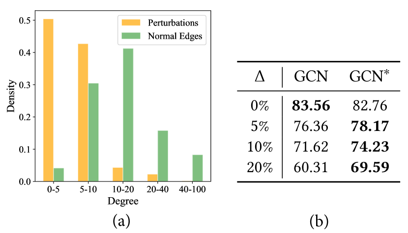
Figure 2. (a): The edge degree distribution of the clean graph and the distribution of the adversarial edges on Cora attacked by MetaAttack. (b): The mean accuracy under different perturbation rates on Cora. The data split follows 10%/ 10%/ 80/%(train/ val/test).

A toy example

GCN assigns higher aggregation weights to low-degree neighbors, and the renormalization adjacency matrix is formulated as: $\hat{\mathbf{A}}=(\textbf{D}+\textbf{I}_{N})^{-\frac{1}{2}}(\mathbf{A}+\textbf{I}_{N})(\textbf{D}+\textbf{I}_{N})^{-\frac{1}{2}}$. However, based on the above analysis, low-degree neighbors are more likely to be maliciously added neighbors. To give a specific example, here is node $v_{i}$ with only one neighbor in the clean graph, and the attacker link it to a low-degree node. In the aggregation step, only half of the messages are are correct. Even worse, the misleading message is assigned a higher weight because the added neighbor has a lower degree than the original neighbor.

Hence, a simple but effective way to improve the robustness of GCN is to assign lower weights to the low-degree neighbors. We propose our advanced GCN, which will implement the message passing as follow:

(12) $$\bm{h}_{i}^{t}=\textrm{ReLU}\Bigl{(}\bigl{(}\sum_{j\in\mathcal{N}_{i}^{*}}\frac{(d_{i}d_{j})^{\alpha}}{Z}\bm{h}_{j}^{t-1}+\beta\bm{h}_{i}^{(t-1)}\bigr{)}\mathbf{W}_{\theta}^{t}\Bigr{)}$$

where $\alpha$ is the hyper-parameter that controls the weight design scheme, $\beta$ is the hyper-parameter that controls the weight of self-loop, $Z$ is a normalization coefficient, and $\textrm{ReLU}(\cdot)=max(0,\cdot)$. $h_{i}^{0}$ is the representation learned in Section 3.2. When $\alpha$ is large, a node aggregate more from the high-degree nodes. $\beta$ is also designed for robustness. Once the neighbors are unreliable, nodes should refer more to themselves.

High-degree nodes can be viewed as robust nodes, because a few perturbations can hardly cancel out the helpful information brought by their original neighbors. The learnable attack algorithms tend to bypass them. Thus, the message from these nodes are usually more reliable.

We show an example in Fig. 2 (b). $\textrm{GCN}^{*}$ denotes the advanced GCN with $\alpha=0.6$ and $\beta=2$. As the perturbation rate increases, the robustness improves more obviously. In fact, this normalization trick can merge with any GNNs.

We train an advanced GCN $f_{\theta}$ by minimizing the cross-entropy:

(13) $$\mathcal{L}_{G}=\sum_{i\in\mathcal{V}_{L}}\ell(f_{\theta}(\textbf{H},\mathbf{A}^{*})_{i},y_{i})$$

where $\ell$ is the cross entropy loss.

Table 2. Classification accuracy(%) under different perturbation rates. The top two performance is highlighted in bold and underline.

Dataset	Ptb Rate	GCN	RGCN	Jaccard	GNNGuard	GRCN	ProGNN	SimPGCN	Elastic	STABLE
Cora	0%	83.56$\pm$0.25	83.85$\pm$0.32	81.79$\pm$0.37	78.52$\pm$0.46	86.12$\pm$0.41	84.55$\pm$0.30	83.77$\pm$0.57	84.76$\pm$0.53	85.58$\pm$0.56
	5%	76.36$\pm$0.84	76.54$\pm$0.49	80.23$\pm$0.74	77.96$\pm$0.54	80.78$\pm$0.94	79.84$\pm$0.49	78.98$\pm$1.10	82.00$\pm$0.39	81.40$\pm$0.54
	10%	71.62$\pm$1.22	72.11$\pm$0.99	74.65$\pm$1.48	74.86$\pm$0.54	72.43$\pm$0.78	74.22$\pm$0.31	75.07$\pm$2.09	76.18$\pm$0.46	80.49$\pm$0.61
	15%	66.37$\pm$1.97	65.52$\pm$1.12	74.29$\pm$1.11	74.15$\pm$1.64	70.72$\pm$1.13	72.75$\pm$0.74	71.42$\pm$3.29	74.41$\pm$0.97	78.55$\pm$0.44
	20%	60.31$\pm$1.98	63.23$\pm$0.93	73.11$\pm$0.88	72.03$\pm$1.11	65.34$\pm$1.24	64.40$\pm$0.59	68.90$\pm$3.22	69.64$\pm$0.62	77.80$\pm$1.10
Citeseer	0%	74.63$\pm$0.66	75.41$\pm$0.20	73.64$\pm$0.35	70.07$\pm$1.31	75.65$\pm$0.21	74.73$\pm$0.31	74.66$\pm$0.79	74.86$\pm$0.53	75.82$\pm$0.41
	5%	71.13$\pm$0.55	72.33$\pm$0.47	71.15$\pm$0.83	69.43$\pm$1.46	74.47$\pm$0.38	72.88$\pm$0.32	73.54$\pm$0.92	73.28$\pm$0.59	74.08$\pm$0.58
	10%	67.49$\pm$0.84	69.80$\pm$0.54	69.85$\pm$0.77	67.89$\pm$1.09	72.27$\pm$0.69	69.94$\pm$0.45	72.03$\pm$1.30	73.41$\pm$0.36	73.45$\pm$0.40
	15%	61.59$\pm$1.46	62.58$\pm$0.69	67.50$\pm$0.78	69.14$\pm$0.84	67.48$\pm$0.42	62.61$\pm$0.64	69.82$\pm$1.67	67.51$\pm$0.45	73.15$\pm$0.53
	20%	56.26$\pm$0.99	57.74$\pm$0.79	67.01$\pm$1.10	69.20$\pm$0.78	63.73$\pm$0.82	55.49$\pm$1.50	69.59$\pm$3.49	65.65$\pm$1.95	72.76$\pm$0.53
Polblogs	0%	95.04$\pm$0.11	95.38$\pm$0.14	/	/	94.89$\pm$0.24	95.93$\pm$0.17	94.86$\pm$0.46	95.57$\pm$0.26	95.95$\pm$0.27
	5%	77.55$\pm$0.77	76.46$\pm$0.47	/	/	80.37$\pm$0.46	93.48$\pm$0.54	75.08$\pm$1.08	90.08$\pm$1.06	93.80$\pm$0.12
	10%	70.40$\pm$1.13	70.35$\pm$0.40	/	/	69.72$\pm$1.36	85.81$\pm$1.00	68.36$\pm$1.88	84.05$\pm$1.94	92.46$\pm$0.77
	15%	68.49$\pm$0.49	67.74$\pm$0.50	/	/	66.56$\pm$0.93	75.60$\pm$0.70	65.02$\pm$0.74	72.17$\pm$0.74	90.04$\pm$0.72
	20%	68.47$\pm$0.54	67.31$\pm$0.24	/	/	68.20$\pm$0.71	73.66$\pm$0.64	64.78$\pm$1.33	71.76$\pm$0.92	88.46$\pm$0.33
Pubmed	0%	86.83$\pm$0.06	86.02$\pm$0.08	86.85$\pm$0.09	85.24$\pm$0.07	86.72$\pm$0.03	87.33$\pm$0.18	88.12$\pm$0.17	87.71$\pm$0.06	87.73$\pm$ 0.11
	5%	83.18$\pm$0.06	82.37$\pm$0.12	86.22$\pm$0.08	84.65$\pm$0.09	84.85$\pm$0.07	87.25$\pm$0.09	86.96$\pm$0.18	86.82$\pm$0.13	87.59$\pm$0.08
	10%	81.24$\pm$0.17	80.12$\pm$0.12	85.64$\pm$0.08	84.51$\pm$0.06	81.77$\pm$0.13	87.25$\pm$0.09	86.41$\pm$0.34	86.78$\pm$0.11	87.46$\pm$0.12
	15%	78.63$\pm$0.10	77.33$\pm$0.16	84.57$\pm$0.11	84.78$\pm$0.10	77.32$\pm$0.13	87.20$\pm$0.09	85.98$\pm$0.30	86.36$\pm$0.14	87.38$\pm$0.09
	20%	77.08$\pm$0.2	74.96$\pm$0.23	83.67$\pm$0.08	84.25$\pm$0.07	69.89$\pm$0.21	87.09$\pm$0.10	85.62$\pm$0.40	86.04$\pm$0.17	87.24$\pm$0.08

4. Experiments

In this section, we empirically analyze the robustness and effectiveness of STABLE against different types of adversarial attacks. Specifically, we aim to answer the following research questions:

• $\mathbf{RQ1}$: Does STABLE outperform the state-of-the-art defense models under different types of adversarial attacks?

• $\mathbf{RQ2}$: Is the structure learned by STABLE better than learned by other methods?

• $\mathbf{RQ3}$: What is the performance with respect to different training parameters?

• $\mathbf{RQ4}$: How do the key components benefit the robustness? (see Appendix A.5)

4.1. Experimental Settings

4.1.1. Datasets

Following  (Zügner et al., 2018; Jin et al., 2020b; Entezari et al., 2020), we conduct our experiments on four benchmark datasets, including three citation graphs, i.e., Cora, Citeseer, and PubMed, and one blog graph, i.e., Polblogs. The statistics of these datasets are shown in Appendix A.2.

4.1.2. Baselines

We compare STABLE with representative and state-of-the-art defence GNNs to verify the robustness. The baselines and SOTA approaches are GCN (Kipf and Welling, 2017), RGCN (Zhu et al., 2019), Jaccard (Wu et al., 2019), GNNGuard (Zhang and Zitnik, 2020), GRCN (Yu et al., 2020), ProGNN (Jin et al., 2020b), SimpGCN (Jin et al., 2021), Elastic (Liu et al., 2021b). We implement three non-targeted structural adversarial attack methods, i.e., MetaAttack (Zügner and Günnemann, 2019), DICE (Waniek et al., 2018) and Random.

We introduce all these defence methods and attack methods in the Appendix A.3.

4.1.3. Implementation Details

The implementation details and parameter settings are introduced in Appendix A.4

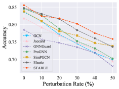
(a) $\textrm{Cora}_{\textrm{DICE}}$

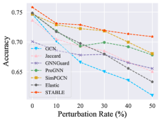
(b) $\textrm{Citeseer}_{\textrm{DICE}}$

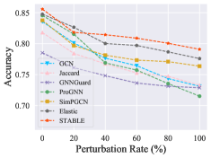
(c) $\textrm{Cora}_{\textrm{Random}}$

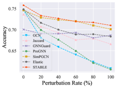
(d) $\textrm{Citeseer}_{\textrm{Random}}$

Figure 3. Cora and Citeseer under DICE and Random

4.2. Robustness Evaluation ($\mathbf{RQ1}$)

To answer $\mathbf{RQ1}$, we evaluate the performance of all methods attacked by different methods.

4.2.1. Against Mettack

Table 2 shows the performance on three datasets against MetaAttack (Zügner and Günnemann, 2019), which is an effective attack method. The top two performance is highlighted in bold and underline. We set the perturbation rate from 0% to 20%. From this main experiment, we have the following observations:

• All the methods perform closely on clean graphs because most of them are designed for adversarial attacks, and the performance on clean graphs is not their goal. Both GCN and RGCN perform poorly on graphs with perturbations, proving that GNNs are vulnerable without valid defenses.

• Jaccard, GNNGuard, GRCN, and ProGNN are all structure learning methods. Jaccard and GNNGuard seem insensitive to the perturbations, but there is a trade-off between the performance and the robustness. They prune the edges based on the features, but the raw features cannot sufficiently represent nodes’ various properties. ProGNN and GRCN perform well when the perturbation rate is low, and the accuracy drops rapidly as the perturbation rate rises. GRCN suffers from poor end-to-end representations, and for ProGNN, we guess it is hard to optimize the structure on a heavily contaminated graph directly. Compared with them, STABLE leverages the task-irrelevant representations to optimize the graph structure, which leads to higher performance.

• SimPGCN and Elastic are two recent state-of-the-art robust methods. SimPGCN is shown robust on Cora and Citeseer because it can adaptively balance structure and feature information. It performs poorly on Polblogs due to the lack of feature information, which can also prove that the robustness of SimpGCN relies on the raw features. Hence, it might also face the same problem that the original features miss some valuable information. Elastic benefits from its ability to model local smoothing. Different from them, our STABLE focus on refining the graph structure, and we just design a variant of GCN as the classifier. STABLE outperforms these two methods with 1%$\thicksim$8% improvement under low perturbation rate and 7%$\thicksim$24% improvement under large perturbation rate.

• STABLE outperforms other methods under different perturbation rates. Note that on Polblogs, we randomly remove and add a small portion of edges to generate augmentations. As the perturbation rate increases, the performance drops slowly on all datasets, which demonstrates that STABLE is insensitive to the perturbations. Especially STABLE has a huge improvement over other methods on heavily contaminated graphs.

4.2.2. Other attacks

The performance under DICE and Random is presented in Fig. 3. We only show the results on Cora and Citeseer due to the page limitation. RGCN and GRCN are not competitive, so they are not shown to keep the figure neat. Considering that DICE and Random are not as effective as MetaAttack, we set the perturbation rate higher. The figure shows that STABLE consistently outperforms all other baselines and successfully resists both attacks. Together with the observations from Section 4.2, we can conclude that STABLE outperforms these baselines and is able to defend against different types of attacks.

4.3. Result of Sturcture Learning ($\mathbf{RQ2}$)

To validate the effectiveness of structure learning, we compare the results of structure optimization in STABLE and other metric learning methods. RGCN fails to refine the graph and makes the graph denser, so we exclude it. The statistics of the learned graphs are shown in Table 3. It shows the number of total removed edges, removed adversarial edges, and removed normal edges. Due to the limit of space, we only show results on Cora under MetaAttack.

To ensure a fair comparison, we tune the pruning thresholds in each method to close the number of total removed edges. It can be observed that STABLE achieves the highest pruning accuracy, indicating that STABLE revise the structure more precisely via more reliable representations.

Table 3. The statistics of the removed edges on the learned graph.

Method	Total	Adversarial	Normal	Accuracy(%)
Jaccard	$1,008$	447	561	44.35
GNNGuard	$1,082$	482	600	44.55
STABLE	$1,035$	601	434	58.07

4.4. Parameter Analysis ($\mathbf{RQ3}$)

From our experimental experience, we mainly tune $k$ and $\alpha$ to achieve peak performance. Thus, we alter their values to see how they affect the robustness of STABLE. The sensitivity of other parameters are presented in Appendix A.6. As illustrated in Fig. 4, we conduct experiments on Cora with the perturbation rate of 20% by MetaAttack. It is worth noting that, regardless of the value of k, it is better to add than not to add. Another observation is that even $\alpha=5$, which means nodes almost only aggregate messages from the neighbors with the highest degree, the result is still better than vanilla GCN, i.e., $\alpha=-0.5$.

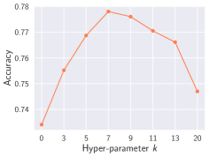
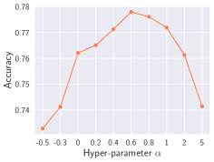
Figure 4. Parameter sensitivity analysis on Cora.

Moreover, to explore the relationship between these parameters and perturbation rates, we list the specific values which achieve the best performance on Cora in Table 4. Both $k$ and $\alpha$ are directly proportional to the perturbation rate, which is consistent with our views. The more poisoned the graph is, the more helpful neighbors are needed, and the more trust in high-degree nodes.

Table 4. The specific values of $k$ and $\alpha$ which achieve the peak performance on Cora under different perturbation rate

Ptb Rate	0%	5%	10%	15%	20%	35%	50%
$k$	1	5	7	7	7	7	13
$\alpha$	-0.5	-0.3	0.3	0.6	0.6	0.7	0.8

5. Related Work

In this section, we present the related literature on robust graph neural networks and graph contrastive learning.

5.1. Robust GNNs

Extensive studies have demonstrated that GNNs are highly fragile to adversarial attacks (Dai et al., 2018; Zügner et al., 2018; Zügner and Günnemann, 2019; Wu et al., 2019; Zhu et al., 2022). The attackers can greatly degrade the performance of GNNs by limitedly modifying the graph data, namely structure and features.

To strengthen the robustness of GNNs, multiple methods have been proposed in the literature, including structure learning (Jin et al., 2020b), adversarial training (Xu et al., 2019a), utilizing Gaussian distributions to represent nodes (Zhu et al., 2019), designing a new message passing scheme driven by $l_{1}$-based graph smoothing (Liu et al., 2021b), combining the kNN graph and the original graph (Jin et al., 2021), and excluding the low-rank singular components of the graph (Entezari et al., 2020).  (Geisler et al., 2020) and  (Chen et al., 2021) study the robustness of GNNs from the breakdown point perspective and propose more robust aggregation approaches.

In the methods mentioned above, one representative type of approach is graph structure learning (Jin et al., 2020b; Zhang and Zitnik, 2020; Luo et al., 2021; Zhu et al., 2021b), which aims to detect the potential adversarial edges and assign these edges lower weights or even remove them. ProGNN (Jin et al., 2020b) and GLNN (Gao et al., 2020) tried to directly optimize the structure by treating it as a learnable parameter, and they introduced some regularizations like sparsity, feature smoothness, and low-rank into the objective.  (Wu et al., 2019) has found that attackers tend to connect two nodes with different features, so they invented Jaccard to prune the edges that link two dissimilar nodes. GNNGuard (Zhang and Zitnik, 2020) also modeled the edge weights by raw features. They further calculated the edge pruning probability through a non-linear transformation. GRCN (Yu et al., 2020) and GAUGM (Zhao et al., 2021) directly computed the weights of the edges by the inner product of representations learned by the classifier, and no additional parameters were needed.

Different from the above-mentioned methods, we aim to leverage task-irrelevant representations, which represent rich properties of nodes and are insensitive to perturbations, to refine the graph structure. Then, we input the well-refined graph into a light robust classifier.

5.2. Graph Contrastive Learning

To learn task-irrelevant representations, we consider using unsupervised methods, which are mainly divided into three categories: GAEs (Kipf and Welling, 2016; Garcia Duran and Niepert, 2017), random walk methods (Jeh and Widom, 2003; Perozzi et al., 2014), and contrastive methods (Veličković et al., 2018; Hassani and Khasahmadi, 2020; Peng et al., 2020; Zhu et al., 2020). Both GAEs and random walk methods are suffer from the proximity over-emphasizing (Veličković et al., 2018), and the augmentation scheme in contrastive methods are naturally similar to adversarial attacks.

Graph contrastive methods are proved to be effective in node classification tasks (Veličković et al., 2018; Hassani and Khasahmadi, 2020; Peng et al., 2020; Zhu et al., 2020). The first such method, DGI (Veličković et al., 2018), transferred the mutual information maximization (Hjelm et al., 2019) to the graph domain. Next, InfoGraph (Sun et al., 2020) modified DGI’s pipeline to make the global representation useful for graph classification tasks. Recently, GRACE (Zhu et al., 2020) and GraphCL (You et al., 2020) adapted the data augmentation methods in vision (Chen et al., 2020a) to graphs and achieved state-of-the-art performance. Specifically, GraphCL generated views by various augmentations, such as node dropping, edge perturbation, attribute masking, and subgraph. However, these augmentations were not designed for adversarial attack scenarios. The edge perturbation method in GraphCL randomly added or deleted edges in the graph, and we empirically prove this random augmentation does not work in Appendix A.5.

Unlike GraphCL and GRACE randomly generated augmentations, STABLE generates robustness-oriented augmentations by a novel recovery scheme, which simulates attacks to make the representations insensitive to the perturbations.

6. Conclusion

To overcome the vulnerability of GNNs, we propose a novel defense model, STABLE, which successfully refines the graph structure via more reliable representations. Further, we design an advanced GCN as a downstream classifier to enhance the robustness of GCN. Our experiments demonstrate that STABLE consistently outperforms state-of-the-art baselines and can defend against different types of attacks. For future work, we aim to explore representation learning in adversarial attack scenarios. The effectiveness of STABLE proves that robust representation might be the key to GNN robustness.

Appendix A APPENDIX

A.1. Algorithm

The overall training algorithm is shown in Algorithm 1. In line 2, we roughly pre-process $\mathcal{G}$ by removing some potential perturbations. From lines 3 to 10, we utilize a contrastive learning model with robustness-oriented augmentations to obtain the node representations. In lines 11 and 12, we refine the graph structure based on the representations learned before. from line 13 to 20, we train the classifier $\textrm{GCN}^{*}$ on $G^{*}$.

Input: Graph $\mathcal{G}=\{\mathcal{V},\mathcal{E},\mathcal{X}\}$, Labels $\mathcal{Y}_{L}$, pre-process threshold $t_{1}$, recovery probability $p$, pruning threshold $t_{2}$, number of adding helpful neighbors $k$, advanced GCN parameters $\alpha$ and $\beta$, training epochs $N_{epoch}$

Output: The predicted labels of $\mathcal{V}_{U}$

1

2Initialize parameters $\phi$, $\omega$ and $\theta$;

3 Roughly pre-process $\mathcal{G}$ to obtain $\mathcal{G}^{P}$ using Eq. (4) and $t_{1}$;

4 Generate augmentations $\mathcal{G}^{P}_{1}$ to $\mathcal{G}^{P}_{M}$ using Eq. (5);

5 Generate $\widetilde{\mathcal{G}}^{P}$ by shuffling the node features of $\mathcal{G}^{P}$;

6 while not converge do

7       Compute H, $\widetilde{\textbf{H}}$, $\textbf{H}_{1}$, $\textbf{H}_{2}$…, and $\textbf{H}_{M}$ using Eq. (6);

8       Compute the global representations of $\mathcal{G}^{P}_{1}$ to $\mathcal{G}^{P}_{M}$ using Eq. (7);

9       Compute the contrastive learning objective using Eq.(8);

10       Update $\phi$ and $\omega$ by $\frac{\partial\mathcal{L}_{C}}{\partial\phi}$ and $\frac{\partial\mathcal{L}_{C}}{\partial\omega}$;

11      

12 end while

13Prune the strcutrue using Eq. (9) and Eq.(10);

14 Add helpful edges using Eq. (11);

15 for e=1, …, $N_{epoch}$ do

16       for t=1, 2 do

17             for $v_{i}\in\mathcal{V}$ do

18                   Compute $h_{i}$ using Eq. (12);

19                  

20             end for

21            

22       end for

23      Compute $\mathcal{L}_{G}$ using Eq. (13);

24       Update $\theta$ by $\frac{\partial\mathcal{L}_{G}}{\partial\theta}$

25 end for

26return argmax($f_{\theta}(\textbf{H},\mathbf{A}^{*})_{\mathcal{V}_{U}}$, dim=1);

Algorithm 1 STABLE

A.2. Datasets

Following  (Zügner et al., 2018; Jin et al., 2020b), we only consider the largest connected connected component (LCC). The statistics is listed in Tabel 5. There is no features available in Polblogs. Following  (Jin et al., 2020b; Liu et al., 2021b) we set the feature matrix to be a $n\times n$ identity matrix. The results of GNNGuard and Jaccard on Polblogs are not available because the cosine similarity of the identity matrix is meaningless. For PubMed dataset, we use the attacked graphs provided provided by (Jin et al., 2020a).

Table 5. Dataset statistics. We only consider the largest connected component (LCC).

Datasets	$\textrm{N}_{\textrm{LCC}}$	$\textrm{E}_{\textrm{LCC}}$	Classes	Features
Cora	2,485	5,069	7	1433
Citeseer	2,110	3,668	6	3703
Polblogs	1,222	16,714	2	/
PubMed	19717	44338	3	500

A.3. Baselines

• GCN (Kipf and Welling, 2017): GCN is a popular graph convolutional network based on spectral theory.

• RGCN (Zhu et al., 2019): RGCN utilizes gaussian distributions to represent node and uses a variance-based attention mechanism to remedy the propagation of adversarial attacks.

• Jaccard (Wu et al., 2019): Since attacks tend to link nodes with different labels, Jaccard prune edges which connect two dissimilar nodes.

• GNNGuard (Zhang and Zitnik, 2020): GNNGuard utilizes cosine similarity to model the edge weights and then calculates edge pruning probability through a non-linear transformation.

• GRCN (Yu et al., 2020): GRCN models edge weights by taking inner product of embeddings of two end nodes.

• ProGNN (Jin et al., 2020b): ProGNN treats the adjacency matrix as learnable parameters and directly optimizes it with three regularizations, i.e., feature smoothness, low-rank and sparsity.

• SimpGCN (Jin et al., 2021): SimpGCN utilizes a $k$NN graph to keep the nodes with similar features close in the representation space and a self-learning regularization to keep the nodes with dissimilar features remote.

• Elastic (Liu et al., 2021b): Elastic introduces $\ell_{1}$-norm to graph signal estimator and proposes elastic message passing which is derived from one step optimization of such estimator. The local smoothness adaptivity enables the Elastic GNNs robust to structural attacks.

• MetaAttack (Zügner and Günnemann, 2019): MetaAttack uses meta-gradients to solve the bilevel problem underlying poisoning attacks, essentially treating the graph as a hyperparameter to optimize.

• DICE (Waniek et al., 2018): Disconnect Internally, connect externally.

• Random: Inject random structure noise.

A.4. Implementation Details

We use DeepRobust, an adversarial attack repository (Li et al., 2020), to implement all the attack methods, RGCN, ProGNN, SimpGCN, and Jaccard. GNNGuard, Elastic, and GCN are implemented with the code provided by the authors.

For each graph, we randomly split the nodes into 10% for training, 10% for validation, and 80% for testing. Then we generate attacks on each graph according to the perturbation rate, and all the hyper-parameters in attack methods are the same with the authors’ implementation. For all the defense models, we report the average accuracy and standard deviation of 10 runs.

All the hyper-parameters are tuned based on the loss and accuracy of the validation set. For RGCN, the hidden dimensions are tuned from {16, 32, 64, 128}. For Jaccard, the Jaccard Similarity threshold are tuned from {0.01, 0.02, 0.03, 0.04, 0.05}. For GNNGuard, we follow the author’s settings, which contains $P_{0}=0.5$, $K=2$, $D_{2}=16$ and $dropout=0.5$. For ProGNN and SimpGCN, following (Jin et al., 2021), we use the default hyper-parameter settings in the authors’ implementation. For Elastic, the propagation step K is tuned from {3, 5, 10}, and the parameter $\lambda_{1}$ and $\lambda_{2}$ are tuned from {0, 3, 6, 9}.

For our work, $t_{1}$ is Jaccard Similarity threshold in this work and tuned from{0.0, 0.01, 0.02, 0.03, 0.04, 0.05}, the recovery portion $p$ is fixed at 0.2, $t_{2}$ is tuned from {0.1, 0.2, 0.3}, $k$ is tuned from {1, 3, 5, 7, 11, 13}, $\alpha$ is tuned from $-0.5$ to $3$, and $\beta$ is fixed at 2. We fix $M=2$ because we find that two augmentation views are good enough. The other parameters in $GCN^{*}$ follows the setting in  (Kipf and Welling, 2017).

A.5. Ablation Study ($\mathbf{RQ4}$)

We conduct an ablation study to examine the contributions of different components in STABLE:

• STABLE-P: STABLE without rough pre-process.

• STABLE-A: STABLE without augmentations.

• STABLE-Ran: STABLE with random augmentations. We generate the views by randomly removing or adding edges.

• STABLE-K: We only prune edges in the refining phase.

• STABLE-GCN: Replace advanced GCN with GCN.

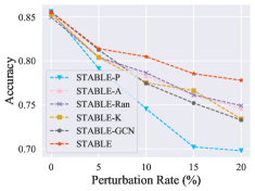
(a) Cora

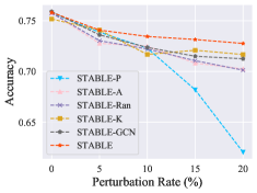
(b) Citeseer

Figure 5. Comparisons between STABLE and its variants.

The accuracy on Cora and Citeseer under MetaAttack is illustrated in Fig. 5. It is clearly observed that the STABLE-P perform worst, and it is in line with our point that $\mathcal{G}^{P}$ is much cleaner than $\mathcal{G}$. STABLE-Ran and STABLE-A perform very closely, and the gap between them and STABLE widens as the perturbation rate increases. We can conclude that the robustness-oriented augmentation indeed works. It is worth noting that STABLE outperforms STABLE-K more significantly as the perturbation rate rising, as our expectation. We argue that adding helpful neighbors can diminish the impact of harmful edges, especially on heavily poisoned graphs.

To further verify the robustness of advanced GCN, we present the performance of SimpGCN* and Jaccard* in Table 6. Jaccard and SimpGCN both contain the vanilla GCN, so we can easily define two variants by replacing the GCN with the advanced GCN. As shown in Table 6, the variants of Jaccard and SimpGCN show more robust than the original models. The improvement of SimpGCN is more significant might because of the pruning strategy in Jaccard, which already removes some adversarial edges.

Table 6. Classification accuracy(%) on Cora under different perturbation rates. The asterisk indicates that the GCN part of this model is replaced with advanced GCN.

Datasets	Ptb rate	Jaccard	Jaccard*	SimpGCN	SimpGCN*
Cora	0%	81.79	81.11	83.77	83.64
	5%	80.23	80.57	78.98	80.45
	10%	74.65	76.99	75.07	78.04
	15%	74.29	76.32	71.42	75.31
	20%	73.11	73.42	68.90	73.29
	35%	66.11	68.79	64.87	71.15
	50%	58.08	64.06	51.94	65.63

A.6. Sensitivity

We explore the sensitivity of $t_{1}$ and $t_{2}$ for STABLE. The performance change of STABLE is illustrate in Figure 6. In fact, for Cora, we fixed $t_{1}$ at 0.03 and $t_{2}$ at 0.2 to achieve the best performance under different perturbation rate. For $t_{1}$, it is worth noting that, the performance on pre-processed graph is consistently higher than on the original graph($t_{1}=0$). $t_{2}=-1$ implies that no edge is pruned in the refining step, and the performance is still competitive might due to the good representations and helpful edge insertions.

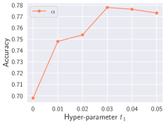
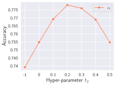
Figure 6. Parameter sensitivity analysis on Cora.