A Multi-stage Framework with Mean Subspace Computation and Recursive Feedback for Online Unsupervised Domain Adaptation

Abstract

In this paper, we address the Online Unsupervised Domain Adaptation (OUDA) problem and propose a novel multi-stage framework to solve real-world situations when the target data are unlabeled and arriving online sequentially in batches. Most of the traditional manifold-based methods on the OUDA problem focus on transforming each arriving target data to the source domain without sufficiently considering the temporal coherency and accumulative statistics among the arriving target data. In order to project the data from the source and the target domains to a common subspace and manipulate the projected data in real-time, our proposed framework institutes a novel method, called an Incremental Computation of Mean-Subspace (ICMS) technique, which computes an approximation of mean-target subspace on a Grassmann manifold and is proven to be a close approximate to the Karcher mean. Furthermore, the transformation matrix computed from the mean-target subspace is applied to the next target data in the recursive-feedback stage, aligning the target data closer to the source domain. The computation of transformation matrix and the prediction of next-target subspace leverage the performance of the recursive-feedback stage by considering the cumulative temporal dependency among the flow of the target subspace on the Grassmann manifold. The labels of the transformed target data are predicted by the pre-trained source classifier, then the classifier is updated by the transformed data and predicted labels. Extensive experiments on six datasets were conducted to investigate in depth the effect and contribution of each stage in our proposed framework and its performance over previous approaches in terms of classification accuracy and computational speed. In addition, the experiments on traditional manifold-based learning models and neural-network-based learning models demonstrated the applicability of our proposed framework for various types of learning models.

I Introduction

Domain Adaptation (DA) [1] has been a research area of growing interest to overcome real-world domain shift issues. The goal of DA is to learn a model from the source domain with sufficient labeled data to maintain the performance of the learned model in the target domain, which has a different distribution from the source domain. The Unsupervised DA (UDA) problem [2, 3, 4, 5], which is a branch of DA problem, assumes that the target data are completely unlabeled, and the Online DA problem [6] tackles the DA problem when a learning system receives streaming target data in an online fashion.

Recently many studies have been conducted on the Online Unsupervised Domain Adaptation (OUDA) problem, which faces the challenges of both online DA and unsupervised DA problems. The OUDA problem assumes that the target data are unlabeled and arriving sequentially in an online fashion. This problem is challenging since it has to overcome the distribution shift between the source and the target domains while the target data is not given as an entire batch. Throughout this paper, we use the term mini-batch to indicate a bunch of consecutive target samples arriving at each timestep.

Early works tackled the OUDA problem by projecting the source and the target data to a manifold. Bitarafan et al. [7] computed a transformation matrix that aligned each arriving target mini-batch closer to the source domain. Target samples are then merged to the source domain once pseudo-labels of those target mini-batches are predicted. Hoffman et al. [8] adopted an additional loss term for optimization that minimized the difference among the target mini-batches at adjacent timesteps. However, these approaches did not sufficiently consider the temporal dependency among the entire sequence of target mini-batches.

Majority of recent studies have tackled the OUDA problem by updating the model as the target mini-batch arrives. Some studies augmented the input data using the pseudo labels of previous target data, while others focused on updating the weights of the neural network based on the statistics (e.g., covariance, entropy etc.) of unlabeled target data. These approaches are valid under the assumption that the target domain shifts gradually [9]. If the source and the target distributions are significantly different, updating the learning system with the target data leads to catastrophic forgetting [10].

Previously, we have proposed a multi-stage framework for the OUDA problem [11], which computes the transformation matrix from target data to the source domain in an online fashion. The framework also considered the accumulative statistics as well as temporal dependency among the entire sequence of target mini-batches. The proposed method incrementally computes the average of the low-dimensional subspaces from the target mini-batches, followed by the computation of a transformation matrix from the mean-target subspace to the source subspace. This transformation matrix aligns the target samples closer to the source domain, which leverages the performance of the model trained on the source domain.

In this paper, we further extend this multi-stage OUDA framework, taking into account the domain shift of the evolving target domain as well as the shift between the source and the target domains. In addition to computing the average subspace of target subspaces on a Grassmann manifold [11], we also consider the flow of the target subspaces on the Grassmann manifold. Utilizing this flow, our proposed framework computes robust mean-target subspaces and precise transformation matrices. The next-target subspace is predicted by extrapolation of the geodesic from previous mean-target subspaces. This prediction technique provides the robustness of online domain adaptation for noisy target subspaces. The recursive feedback stage leverages the performance of our proposed framework by transforming the next arriving target mini-batch. The transformed target mini-batch is represented by a subspace that is closer to the source domain, hence improving the performance of online domain adaptation. In addition, transformation matrix from the target domain to the source domain is computed cumulatively, considering intermediate domains between the source and the successive target subspaces. Moreover, the classifier in our proposed framework is adaptive, whereas the source classifier in our previous work [11] is not changing. This adaptive classifier leverages the performance of online adaptation by including the knowledge from the arriving target data.

We also validate the efficiency of the incremental mean-target-subspace computation technique on a Grassmann manifold, called an Incremental Computation of Mean-Subspace (ICMS) [11]. We have also proved that the computed mean-subspace is close to the Karcher mean [12] – one of the most common and efficient methods related to the mean on manifolds – while maintaining significantly low-computational burden as compared to the Karcher-mean computation. We have also empirically shown in experiments that ICMS is faster than the Karcher-mean computation. This efficient computation of a close approximate to the Karcher mean makes the online feedback computation of the OUDA problem possible. Extensive computer simulations were performed to validate and analyze the proposed multi-stage OUDA framework. In the computer simulations, we further analyzed in depth each stage of the proposed framework to investigate how those stages contribute to solving the OUDA problem.

In summary, the contributions of this paper are efficient computation of mean-target subspace on a Grassmann manifold, robustness on noisy online domain adaptation task using recursive feedback and next-target-subspace prediction, consideration of cumulative temporal consistency using the flow of target domain on the Grassmann manifold, and adaptivity of classifier that is suitable for online domain adaptation.

The remainder of this paper is organized as follows. Section II briefly introduces related works. Section III formally describes the OUDA problem and our proposed multi-stage OUDA framework for solving it. Section IV describes the details of the proposed ICMS computation as well as the mathematical proof of subspace convergence. Section V describes the experimental simulations and results, and Section VI summarizes the findings and conclusions of the paper.

II Related Work

Among many approaches proposed for the UDA problem, the subspace-based approaches for the UDA problem focused on the alignment of the projected data on a common subspace of the source and the target domains. Long et al. [13] proposed the concept of Maximum Mean Discrepancy (MMD) –  a metric that minimized the distance between mean points on Reproducing Kernel Hilbert Spaces (RHKS) [14]. Fernando et al. [4] suggested the Subspace Alignment (SA) technique that aligned the subspaces of the source and the target domains, and then minimized the distance between these two domains.

Other approaches utilized a common subspace to project the data from the source and the target domains, but they did not directly align the projected data. Gong et al. [2] proposed a Geodesic Flow Kernel (GFK) technique that computed a transform matrix using a kernel-based method. This transform matrix characterizes the transformation of the original data from the target domain to the source domain on a Grassmann manifold.

Other previous work attempted to align the source and the target domains by directly minimizing their statistical properties. Sun et al. [15] adopted a Correlation Alignment (CORAL) approach that minimized the domain discrepancy directly on the original data space by adjusting the second-order statistics of the source and the target distributions. Zhang et al. [3] suggested the Joint Geometrical and Statistical Alignment (JGSA) technique  –  a combined technique of MMD and SA methods. Wang et al. [16] proposed a Manifold Embedded Distribution Alignment (MEDA) approach that quantitatively evaluated the marginal and conditional distributions in domain adaptation. Vascon et al. [5] formulated the UDA problem as a semi-supervised incremental learning problem using the Game Theory and suggested a Graph Transduction for Domain Adaptation (GTDA) method. The GTDA method obtained the optimal classification result on the target domain using Nash equilibrium [17]. Wulfmeier et al. [18] adopted Generative Adversarial Networks (GANs) [19] to align the features across domains.

Recently, more studies on the OUDA problem have emerged. Wulfmeier et al. [20] extended their previous work [18] on the UDA problem to the online case using a GAN-based approach. Unfortunately, their approach was not applicable to real-time situations since it requires the training stage of the target data. Bitarafan et al. [7] proposed an Incremental Evolving Domain Adaptation (EDA) technique that consisted of the target data transformation using GFK followed by the source-subspace update using Incremental Partial Least Square (IPLS) [21]. Hoffman et al. [8] proposed another approach for the OUDA problem, using Continuous-Manifold-based Adaptation (CMA) that formulated the OUDA problem as a non-convex optimization problem. Liu et al. [22] suggested a meta-adaptation framework that utilized meta-learning [23] to tackle the OUDA problem. More recently, Kumar et al. [9] theoretically studied gradual domain adaptation, where the goal was to adapt the source classifier given unlabeled target data that shift gradually in distribution. They proved that self-training leverages the gradual domain adaptation with small Wasserstein-infinity distance.

Other studies have focused on the applications of the OUDA problem. Mancini et al. [24] adopted a Batch Normalization [25] (BN) technique to tackle the OUDA problem for a robot kitting task. Wu et al. [26] tackled the OUDA problem using memory store and meta-learning on a semantic segmentation task. Xu et al. [27] suggested an online domain adaptation method for Deformable Part-based Model (DPM), which is applicable for Multiple Object Tracking (MOT).

More recently, there have been many studies on tackling the test-time adaptation task with neural-network-based models. The test-time adaptation task, in addition to the OUDA problem setting, assumes that the source data is not accessible during the test time. The NN-based approaches tackled this task by updating the model parameters online as unlabeled target data arrives. Bobu et al. [10] proposed a replay method to overcome catastrophic forgetting in neural networks. Wu et al. [28] suggested the Online Gradient Descent (OGD) and Follow The History (FTH) techniques for tackling the OUDA problem. Sun et al. [29] proposed the Test-Time-Training (TTT) approach that utilizes self-supervised auxiliary task to solve the OUDA problem. They rotated the test images by 0, 90, 180 and 270 degrees and had the model predicted the angle of rotation as a four-way classification problem. Schneider et al. [30] removed the covariate shift between the source and the target distribution by batch normalization. Wang et al. [31] updated the model by minimizing the entropy loss of the unlabeled target data.

III Proposed Approach

III-A Problem Description

The OUDA problem assumes that the source-domain data are labeled while the target data are unlabeled and arriving online in a sequence of mini-batches at each timestep. As shown in Fig. 1, the goal of the OUDA problem is to classify the arriving unlabeled target mini-batches with the model pre-trained by the source data. Formally, the samples in the source domain $\mathbf{X}_{\mathcal{S}}\in\mathbb{R}^{N_{\mathcal{S}}\times d}$ are given and labeled as $\mathbf{Y}_{\mathcal{S}}\in\mathbb{R}^{N_{\mathcal{S}}\times c}$, where $N_{\mathcal{S}}$, $d$, and $c$ indicate the number of source data, the dimension of the data and the number of class categories, respectively. The target data $\mathbf{X}_{\mathcal{T}}=\{\mathbf{X}_{\mathcal{T},1},\mathbf{X}_{\mathcal{T},2},\cdots,\mathbf{X}_{\mathcal{T},B}\}$ in the target domain $\mathcal{T}$ are a sequence of unlabeled mini-batches that arrive in an online fashion, where $B$ indicates the number of mini-batches. As mentioned previously, we use the term mini-batch for the $n^{th}$ target-data batch $\mathbf{X}_{\mathcal{T},n}\in\mathbb{R}^{N_{\mathcal{T}}\times d}$, where $N_{\mathcal{T}}$ indicates the number of data in each mini-batch. Subscript $(\mathcal{T},n)$ represents the $n^{th}$ mini-batch in the target domain. $N_{\mathcal{T}}$ is assumed to be a constant for $n=1,2,\cdots,B$ and is small compared to $N_{\mathcal{S}}$. Our goal is to transform each target mini-batch $\mathbf{X}_{\mathcal{T},n}$ to $\mathbf{X^{\prime}}_{\mathcal{T},n}$, which is aligned with the source domain $\mathcal{S}$, in an online fashion. The transformed target data $\mathbf{X^{\prime}}_{\mathcal{T},n}$ can be classified correctly as $\mathbf{\hat{Y}}_{\mathcal{T},n}$ with the classifier pre-trained in the source domain $\mathcal{S}$. The nomenclature of our paper is summarized in Table I.

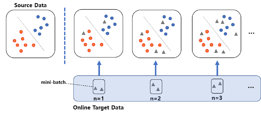
Figure 1: Overview of the OUDA problem. Given the classifier trained with labeled source data (circles) from two classes (orange and blue), the OUDA problem aims to classify the unlabeled target data (grey triangles) arriving online in a mini-batch. Our proposed framework focuses on aligning each target data to the source domain.

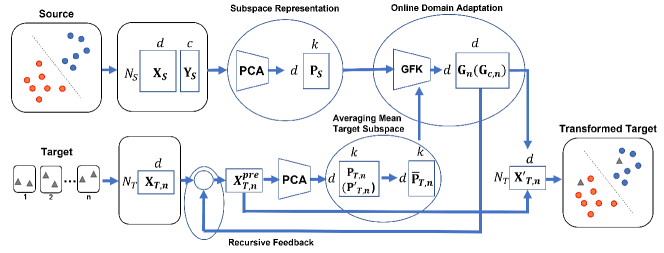
Figure 2: Schematic of the proposed OUDA framework. The proposed framework consists of four stages: 1) Subspace representation, 2) Averaging Mean-target subspace, 3) Online domain adaptation, and 4) Recursive feedback.

TABLE I: Nomenclature of Proposed Framework

Notation	Meaning
$\mathcal{S}$	The source domain
$\mathcal{T}$	The target domain
$N_{\mathcal{S}}$	The number of the source data samples
$N_{\mathcal{T}}$	The number of data samples in a mini-batch
$\mathcal{G}(k,d)$	$k$-dimensional Grassmann manifold of $\mathbb{R}^{d}$
$\mathbf{X}_{\mathcal{S}}$	The set of source data
$\mathbf{Y}_{\mathcal{S}}$	The source labels
$\mathbf{X}_{\mathcal{T}}$	The set of target data
$\mathbf{X}_{\mathcal{T},i}$	$i^{th}$ target mini-batch
$\mathbf{X^{\prime}}_{\mathcal{T}}$	The set of transformed target data
$\mathbf{X^{\prime}}_{\mathcal{T},i}$	$i^{th}$ transformed target mini-batch
$\mathbf{X}^{\prime}_{\mathcal{T},i}$	Transformed $i^{th}$ target mini-batch
$\mathbf{X}^{pre}_{\mathcal{T},n}$	The pre-processed $n^{th}$ target mini-batch
$\mathbf{P}_{\mathcal{S}}$	The source subspace of the source data
$\mathbf{P}_{\mathcal{T},i}$	The target subspace of $i^{th}$ target mini-batch
$\mathbf{P^{\prime}}_{\mathcal{T},n}$	Compensated target subspace by subspace prediction
$\mathbf{\overline{P}}_{\mathcal{T},i}$	Mean-target subspace of $i$ subspaces $\mathbf{P}_{\mathcal{T},1},\mathbf{P}_{\mathcal{T},2},\cdots,\mathbf{P}_{\mathcal{T},i}$
$\mathbf{G}_{n}$	Transformation matrix that transforms $\mathbf{X}_{\mathcal{T},i}$
$\mathbf{G}_{c,n}$	Cumulative transformation matrix that transforms $\mathbf{X}_{\mathcal{T},i}$

III-B Preliminaries: Grassmann Manifold

Throughout this paper, we utilize a Grassmann manifold $\mathcal{G}(k,d)$ [32] –  a space that parameterizes all $k$-dimensional linear subspaces of $d$-dimensional vector space $\mathbb{R}^{d}$. A single point on $\mathcal{G}(k,d)$ represents a subspace that does not depend on the choice of basis. Formally, for a $d\!\times\!k$ matrix $\mathbf{P}$ of full rank $k$ and any nonsingular $k\!\times\!k$ matrix $\mathbf{L}$, the column space col($\mathbf{P}$) of set $\mathbf{A}=\{\mathbf{PL}|\mathbf{P}\in\mathcal{V}(k,d),\mathbf{L}\in SO(k)\}$ is a single point on $\mathcal{G}(k,d)$, where $\mathcal{V}(k,d)$ is a point on Stiefel manifold [33] and $SO(k)$ is a special orthogonal group [32]. For simplicity of notation, we denote this point col($\mathbf{P}$) as corresponding basis $\mathbf{P}\in\mathbb{R}^{d\times k}$ throughout this manuscript.

III-C Proposed OUDA Framework

The proposed OUDA framework consists of four stages for processing an incoming $n^{th}$ mini-batch target data: 1) Subspace representation, 2) Averaging mean-target subspace, 3) Online domain adaptation, and 4) Recursive feedback as shown in Fig. 2. Instead of utilizing the raw samples from both source and target domains, Stage one embeds those samples $\mathbf{X}_{\mathcal{S}}$ and $\mathbf{X}_{\mathcal{T},n}$ to low-dimensional subspaces (i.e. $k$-dimensional subspace of $\mathbb{R}^{d}$) $\mathbf{P}_{\mathcal{S}}$ and $\mathbf{P}_{\mathcal{T},n}$, respectively, for faster computation of transformation matrix from the target domain $\mathcal{T}$ to the source domain $\mathcal{S}$.

Stage two computes the mean of target subspaces $\mathbf{\overline{P}}_{\mathcal{T},n}$ embedded in a Grassmann manifold using our novel Incremental Computation of Mean Subspace (ICMS) method. The proposed ICMS technique is an efficient method of computing the mean of target subspaces and its computed mean is a valid approximate of the Karcher mean [12]. The $n^{th}$ target subspace $\mathbf{P}_{\mathcal{T},n}$ can be further compensated as $\mathbf{P^{\prime}}_{\mathcal{T},n}$ by target-subspace prediction as discussed in a later subsection. Stage three is the online domain adaptation and it computes a transform matrix $\mathbf{G}_{n}$ that aligns each arriving target mini-batch to the source domain. $\mathbf{G}_{n}$ can be replaced with the matrix $\mathbf{G}_{c,n}$ that is computed with a cumulative computation technique. Stage four provides recursive feedback by feeding $\mathbf{G}_{n}$ back to the next mini-batch $\mathbf{X}_{\mathcal{T},n+1}$. Each stage is briefly described next.

III-C1 Subspace Representation

The goal of our proposed OUDA framework is to find the transformation matrix $\mathbf{G}=\{\mathbf{G}_{1},\mathbf{G}_{2},\cdots,\mathbf{G}_{B}\}$ that transforms the set of target mini-batches $\mathbf{X}_{\mathcal{T}}=\{\mathbf{X}_{\mathcal{T},1},\mathbf{X}_{\mathcal{T},2},\cdots,\mathbf{X}_{\mathcal{T},B}\}$ to $\mathbf{X^{\prime}}_{\mathcal{T}}=\{\mathbf{X^{\prime}}_{\mathcal{T},1},\mathbf{X^{\prime}}_{\mathcal{T},2},\cdots,\mathbf{X^{\prime}}_{\mathcal{T},B}\}$ so that the transformed target data $\mathbf{X^{\prime}}_{\mathcal{T},n}=\mathbf{X}_{\mathcal{T},n}\mathbf{G}_{n}$ ($n=1,2,\cdots,B$) are well aligned to the source domain, where $\mathbf{G}_{n}\in\mathbb{R}^{d\times d}$ indicates the transformation matrix from $\mathbf{X}_{\mathcal{T},n}$ to $\mathbf{X^{\prime}}_{\mathcal{T},n}$. Since all the computations must be conducted online, we prefer not to use methods that compute $\mathbf{G}_{n}$ directly on the original high-dimensional data space. Hence, we embed those samples, $\mathbf{X}_{\mathcal{S}}$ and $\mathbf{X}_{\mathcal{T},n}$, in low-dimensional subspaces $\mathbf{P}_{\mathcal{S}}=f(\mathbf{X}_{\mathcal{S}})\in\mathbb{R}^{d\times k}$ and $\mathbf{P}_{\mathcal{T},n}=f(\mathbf{X}_{\mathcal{T},n})\in\mathbb{R}^{d\times k}$, respectively, where $d$ represents the dimension of the original data and $k$ represents the dimension of the subspace. As mentioned above, we represent the subspace as a corresponding basis matrix. $f(\cdot)$ can be any low-dimensional representation, but in this paper we adopt the Principal Component Analysis (PCA) algorithm [34] to obtain $\mathbf{P}_{\mathcal{S}}$ and $\mathbf{P}_{\mathcal{T}}$ since it is simple and fast for online domain adaptation and is suitable for both labeled and unlabeled data.

III-C2 Averaging Mean-target Subspace

Since a subspace is represented as a single point on a Grassmann manifold, $\mathbf{P}_{\mathcal{S}}$ and $\mathbf{P}_{\mathcal{T},1},\mathbf{P}_{\mathcal{T},2},\cdots,\mathbf{P}_{\mathcal{T},n}$ are represented as $(n+1)$ points on $\mathcal{G}(k,d)$. Since all the samples in the source domain $\mathcal{S}$ are given, $\mathbf{X}_{\mathcal{S}}$ can be compressed to a low-dimensional subspace $\mathbf{P}_{\mathcal{S}}$ by conducting the embedding technique only once. For the target domain $\mathcal{T}$, however, each mini-batch $\mathbf{X}_{\mathcal{T},n}$ should be represented as a low-dimensional subspace $\mathbf{P}_{\mathcal{T},n}$ in every timestep as it arrives. Since a single mini-batch is assumed to contain a small number of the target samples (i.e., $N_{\mathcal{T}}$ is small), it does not sufficiently represent the target domain.

To find a subspace that generalizes the target domain $\mathcal{T}$, we compute the mean-target subspace $\mathbf{\overline{P}}_{\mathcal{T},n}$ of $n$ target subspaces $\mathbf{P}_{\mathcal{T},1},\mathbf{P}_{\mathcal{T},2},\cdots,\mathbf{P}_{\mathcal{T},n}$. Traditionally, Karcher mean [12] is utilized as the mean of subspaces represented on a Grassmann manifold. Unfortunately, computing the Karcher mean is an iterative process, which is not suitable for online domain adaptation. Thus, we propose a novel computation technique, called Incremental Computation of Mean-Subspace (ICMS), to compute the mean-target subspace $\mathbf{\overline{P}}_{\mathcal{T},i}$ online for every $i=1,2,\cdots,n,\cdots,B$. Different from the iterative process in computing the Karcher mean, the proposed ICMS technique incrementally computes the mean-target subspace efficiently to satisfy the online computational demand and its computed mean is a close approximate to the Karcher mean. Formally, when the $n^{th}$ mini-batch $\mathbf{X}_{\mathcal{T},n}$ arrives and is represented as a subspace $\mathbf{P}_{\mathcal{T},n}$, we incrementally compute the mean-target subspace $\mathbf{\overline{P}}_{\mathcal{T},n}$ using $\mathbf{P}_{\mathcal{T},n}$ and $\mathbf{\overline{P}}_{\mathcal{T},n-1}$, where $\mathbf{\overline{P}}_{\mathcal{T},n-1}$ is the mean subspace of ($n-1$) target subspaces $\mathbf{P}_{\mathcal{T},1},\mathbf{P}_{\mathcal{T},2},\cdots,\mathbf{P}_{\mathcal{T},n-1}$. We mathematically prove that the computed mean from the ICMS computation is close to the Karcher mean in Section IV. $\mathbf{\overline{P}}_{\mathcal{T},n}$ can be rectified to $\mathbf{\overline{P}^{\prime}}_{\mathcal{T},n}$ using the next-target subspace prediction, which is described in Section IV-D.

III-C3 Online Domain Adaptation

After the mean-target subspace $\mathbf{\overline{P}}_{\mathcal{T},n}$ is computed using the proposed ICMS technique, we compute the transformation matrix $\mathbf{G}_{n}$ that transforms the mini-batch $\mathbf{X}_{\mathcal{T},n}$ to $\mathbf{X^{\prime}}_{\mathcal{T},n}$, where $\mathbf{X^{\prime}}_{\mathcal{T},n}=\mathbf{X}_{\mathcal{T},n}\mathbf{G}_{n}$. We adopt the method proposed by Bitarafan et al. [7] to compute the matrix $\mathbf{G}_{n}$ from $\mathbf{\overline{P}}_{\mathcal{T},n}$ and the source subspace $\mathbf{P}_{\mathcal{S}}$ using the GFK method [2]. The transformed mini-batch $\mathbf{X^{\prime}}_{\mathcal{T},n}$ is aligned closer to the source domain $\mathcal{S}$ compared to the original mini-batch $\mathbf{X}_{\mathcal{T},n}$. This $\mathbf{X^{\prime}}_{\mathcal{T},n}$ is classified by the classifier pre-trained with the samples from the source domain $\mathcal{S}$. Note that $\mathbf{G}_{n}\in\mathbb{R}^{d\times d}$ transforms the original mini-batch $\mathbf{X}_{\mathcal{T},n}$ and not the subspace $\mathbf{P}_{\mathcal{T},n}$. We exploit this $\mathbf{G}_{n}$ when the $(n+1)^{th}$ mini-batch $\mathbf{X}_{\mathcal{T},n+1}$ arrives. $\mathbf{G}_{n}$ can be replaced with the transformation matrix $\mathbf{G}_{c,n}$, which is obtained by cumulative computation and is described in Section IV-F.

III-C4 Recursive Feedback

Followed by the computation of the transformation matrix, we institute a recursive feedback stage that applies the transformation matrix to the next target mini-batch before inputting it to the subspace representation stage. This feedback stage aligns the next target mini-batch closer to the source domain before inputting into the subspace representation stage, which leverages the performance of adaptation. It is crucial to note that the feedback stage at time step $n$ affects the $(n+1)^{th}$ target mini-batch. Formally, we feed $\mathbf{G}_{n}$ back to $\mathbf{X}_{\mathcal{T},n+1}$ as $\mathbf{X}^{pre}_{\mathcal{T},n+1}=\mathbf{X}_{\mathcal{T},n+1}\mathbf{G}_{n}$ before inputting $\mathbf{X}_{\mathcal{T},n+1}$ to the first stage of the proposed OUDA framework. The pre-processed target data $\mathbf{X}^{pre}_{\mathcal{T},n+1}$ is aligned closer to the source subspace $\mathcal{S}$ than $\mathbf{X}_{\mathcal{T},n+1}$. Combined with next-target subspace prediction, the recursive feedback stage leverages the performance of online domain adaptation when the target domains are noisy. In the next section, we describe the detailed procedure of the proposed ICMS technique and online domain adaptation.

IV Incremental Computation of Mean-Subspace for Online Domain Adaptation

The main contribution of the proposed OUDA framework is the ICMS computation technique followed by online domain adaptation. The proposed ICMS technique incrementally computes the mean-target subspace efficiently on a Grassmann manifold and its computed mean is close to the Karcher mean. The proposed ICMS computation also satisfies the online computational demand of the OUDA problem.

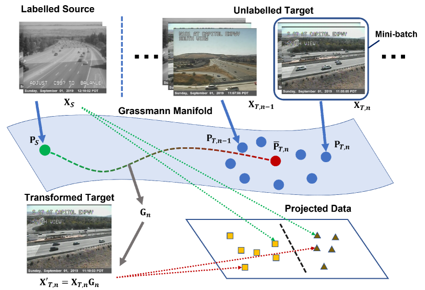
Figure 3: Detailed schematic of the proposed ICMS technique. As the mean-target subspace $\mathbf{\overline{P}}_{\mathcal{T},n}$ (red dot) is computed, the geodesic flow from $\mathbf{P}_{\mathcal{S}}$ (green dot) to $\mathbf{\overline{P}}_{\mathcal{T},n}$ is obtained for computing the transformation matrix $\mathbf{G}_{n}$ (grey arrow). Transformed target data $\mathbf{X^{\prime}}_{\mathcal{T},n}$ are then projected (red arrow) to a projective space, where the source data $\mathbf{X}_{\mathcal{S}}$ are projected (green arrow).

Figure 3 shows the detailed schematic of the proposed ICMS technique. In Fig. 3, as the $n^{th}$ target mini-batch $\mathbf{X}_{\mathcal{T},n}$ is represented as the $n^{th}$ target subspace $\mathbf{P}_{\mathcal{T},n}$ on a Grassmann manifold, the mean-target subspace $\mathbf{\overline{P}}_{\mathcal{T},n}$ is efficiently computed on the Grassmann manifold. The transformation matrix $\mathbf{G}_{n}$ is computed from the mean-target subspace $\mathbf{\overline{P}}_{\mathcal{T},n}$ and the source subspace $\mathbf{P}_{\mathcal{S}}$. Using this transformation matrix $\mathbf{G}_{n}$, the transformed target data $\mathbf{X^{\prime}}_{\mathcal{T},n}$ is aligned with the source domain. With this alignment, the classifier trained on the source data performs well for the arriving target data.

We first review the geodesic flow on a Grassmann manifold, and then discuss the derivation and computation of ICMS and its convergence, and finally its utilization for online domain adaptation.

IV-A Geodesic Flow on a Grassmann Manifold

A geodesic is the shortest-length curve between two points on a manifold [35]. The geodesic flow on a Grassmann manifold $\mathcal{G}(k,d)$ that starts from a point $\mathbf{P}_{1}$ is given by $\mathbf{\Phi}(t)=\mathbf{Q}\exp{(t\mathbf{B})}\mathbf{J}$, where the matrix $\mathbf{Q}=[\mathbf{P}_{1}\>\>\>\mathbf{R}_{1}]\in SO(d)$, and $\mathbf{Q}$ is termed as an Orthogonal Completion of $\mathbf{P}_{1}$ such that $\mathbf{Q}^{T}\mathbf{P}_{1}=\mathbf{J}$ and $\mathbf{J}=\begin{bmatrix}\mathbf{I}_{k}\\ \mathbf{O}_{d-k,k}\end{bmatrix}$. Here the matrices $\mathbf{I}_{k}$ and $\mathbf{O}_{d-k,k}$ denote $k\!\times\!k$ identity matrix and $(d-k)\!\times\!k$ zero matrix, respectively. Using the geodesic parameterization with a single parameter $t$ [35], the geodesic flow from $\mathbf{P}_{1}$ to $\mathbf{P}_{2}$ on a Grassmann manifold $\mathcal{G}(k,d)$ is parameterized as $\mathbf{\Psi}\!:t\in[0,1]\xrightarrow{}\mathbf{\Psi}(t)\in\mathcal{G}(k,d)$:

$$\mathbf{\Psi}(t)=\mathbf{P}_{1}\mathbf{U}_{1}\mathbf{\Gamma}(t)-\mathbf{R}_{1}\mathbf{U}_{2}\mathbf{\Sigma}(t)$$ (1)

under the two constraints that $\mathbf{\Psi}(0)=\mathbf{P}_{1}$ and $\mathbf{\Psi}(1)=\mathbf{P}_{2}$, where $\mathbf{\Gamma}(t)$ and $\mathbf{\Sigma}(t)=[\mathbf{\Sigma}_{1}(t)^{T}\text{ }\mathbf{O}^{T}]^{T}$ are diagonal and block diagonal matrices whose elements are $\cos{(t\theta_{i,n})}$ and $\sin{(t\theta_{i,n})}$, respectively. $\mathbf{R}_{1}$ denotes the orthogonal complement to $\mathbf{P}_{1}$, namely $\mathbf{R}_{1}^{T}\mathbf{P}_{1}=\mathbf{O}$. Two orthonormal matrices $\mathbf{U}_{1}\in\mathbb{R}^{k\times k}$ and $\mathbf{U}_{2}\in\mathbb{R}^{(d-k)\times(d-k)}$ are given by the following Generalized Singular-Value Decompositions (GSVD) [36],

$$\mathbf{Q}^{T}\mathbf{P}_{2}=\begin{pmatrix}\mathbf{U}_{1}&\mathbf{0}\\ \mathbf{0}&\mathbf{U}_{2}\end{pmatrix}\begin{pmatrix}\mathbf{\Gamma}(t)\\ \mathbf{-\Sigma}(t)\end{pmatrix}\mathbf{V}^{T},$$ (2)

where $\mathbf{\Gamma}(t)\in\mathbb{R}^{k\times k}$ and $\mathbf{\Sigma}(t)=[\mathbf{\Sigma}_{1}(t)^{T}\text{ }\mathbf{O}^{T}]^{T}\in\mathbb{R}^{(d-k)\times k}$ are diagonal and block diagonal matrices, respectively, and $\mathbf{\Sigma}_{1}(t)\in\mathbb{R}^{k\times k}$ and $\mathbf{O}\in\mathbb{R}^{(d-2k)\times k}$.

IV-B Mean-target Subspace Computation – ICMS

Since computing the Karcher mean is a time-consuming, iterative process and not suitable for online domain adaptation, we propose a novel technique, called Incremental Computation of Mean-Subspace (ICMS), for computing the mean-target subspace of $n$ target subspaces on a Grassmann manifold.

The proposed ICMS is inspired by the geometric interpretation of computing the mean of $n$ points on the Euclidean space. As shown in Fig. 4(a), it is geometrically intuitive to compute the mean point $\mathbf{\overline{X}}_{n}$ of $n$ points $\mathbf{X}_{1},\mathbf{X}_{2},\cdots,\mathbf{X}_{n}$ in an incremental way when the points are on the Euclidean space. If the mean point $\mathbf{\overline{X}}_{n-1}$ of ($n-1$) points $\mathbf{X}_{1},\mathbf{X}_{2},\cdots,\mathbf{X}_{n-1}$ as well as the $n^{th}$ point $\mathbf{X}_{n}$ are given, the updated mean point $\mathbf{\overline{X}}_{n}$ can be computed as $\mathbf{\overline{X}}_{n}=\{(n-1)\mathbf{\overline{X}}_{n-1}+\mathbf{X}_{n}\}/n$. From a geometric perspective, $\mathbf{\overline{X}}_{n}$ is the internal point, where the distances from $\mathbf{\overline{X}}_{n}$ to $\mathbf{\overline{X}}_{n-1}$ and to $\mathbf{X}_{n}$ have the ratio of $1\!:\!(n-1)$:

$$|\mathbf{\overline{X}}_{n-1}\mathbf{\overline{X}}_{n}|=\frac{|\mathbf{\overline{X}}_{n-1}\mathbf{X}_{n}|}{n}.$$ (3)

We adopt this geometric perspective of ratio concept to the Grassmann manifold. However, Eq. (3) is not directly applicable to a Grassmann manifold since the distance between two points on the Grassmann manifold is not an Euclidean distance. In Fig. 4(b), we update the mean-target subspace $\mathbf{\overline{P}}_{\mathcal{T},n}$ of $n$ target subspaces when the previous mean subspace $\mathbf{\overline{P}}_{\mathcal{T},n-1}$ of ($n-1$) target subspaces and the $n^{th}$ subspace $\mathbf{P}_{\mathcal{T},n}$ are given. $\mathbf{\overline{P}}_{\mathcal{T},n}$ is the introspection point that divides the geodesic flow from $\mathbf{\overline{P}}_{\mathcal{T},n-1}$ to $\mathbf{P}_{\mathcal{T},n}$ to the ratio of $1\!:\!(n-1)$. Following Eq. (1), the geodesic flow from $\mathbf{\overline{P}}_{\mathcal{T},n-1}$ to $\mathbf{P}_{\mathcal{T},n}$ is parameterized as $\mathbf{\Psi}_{n}:t\in[0,1]\xrightarrow{}\mathbf{\Psi}_{n}(t)\in G(k,d)$:

$$\mathbf{\Psi}_{n}(t)=\mathbf{\overline{P}}_{\mathcal{T},n-1}\mathbf{U}_{1,n}\mathbf{\Gamma}_{n}(t)-\mathbf{\overline{R}}_{\mathcal{T},n-1}\mathbf{U}_{2,n}\mathbf{\Sigma}_{n}(t)$$ (4)

under the constraints of $\mathbf{\Psi}_{n}(0)\!=\!\mathbf{\overline{P}}_{\mathcal{T},n-1}$ and $\mathbf{\Psi}_{n}(1)\!=\!\mathbf{P}_{\mathcal{T},n}$. $\mathbf{\overline{R}}_{\mathcal{T},n-1}\in\mathbb{R}^{d\times(d-k)}$ denotes the orthogonal complement to $\mathbf{\overline{P}}_{\mathcal{T},n-1}$; that is, $\mathbf{\overline{R}}_{\mathcal{T},n-1}^{T}\mathbf{\overline{P}}_{\mathcal{T},n-1}=\mathbf{0}$. Two orthonormal matrices $\mathbf{U}_{1,n}\in\mathbb{R}^{k\times k}$ and $\mathbf{U}_{2,n}\in\mathbb{R}^{(d-k)\times(d-k)}$ are defined similar to Eq. (2) and given by the following pair of singular-value decompositions (SVDs),

$$\mathbf{\overline{P}}_{\mathcal{T},n-1}^{T}\mathbf{P}_{\mathcal{T},n}=\mathbf{U}_{1,n}\mathbf{\Gamma}_{n}\mathbf{V}_{n}^{T}\>\>$$ (5)

$$\mathbf{\overline{R}}_{\mathcal{T},n-1}^{T}\mathbf{P}_{\mathcal{T},n}=-\mathbf{U}_{2,n}\mathbf{\Sigma}_{n}\mathbf{V}_{n}^{T}$$ (6)

where $\mathbf{\Gamma}_{n}\in\mathbb{R}^{k\times k}$ and $\mathbf{\Sigma}_{n}=[\mathbf{\Sigma}_{1,n}^{T}\text{ }\mathbf{O}^{T}]^{T}\in\mathbb{R}^{(d-k)\times k}$ are diagonal and block diagonal matrices, respectively, and $\mathbf{\Sigma}_{1,n}\in\mathbb{R}^{k\times k}$ and $\mathbf{O}\in\mathbb{R}^{(d-2k)\times k}$.

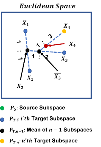
(a)

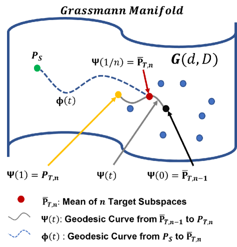
(b)

Figure 4: Mean-target subspace computation.   (a) Geometric interpretation of computing the mean point of $n$ points in the Euclidean space.   (b) Computation of mean-target subspace $\mathbf{\overline{P}}_{\mathcal{T},n}$ on a Grassmann manifold.

When the $n^{th}$ target mini-batch $\mathbf{X}_{\mathcal{T},n}$ arrives and is represented as the subspace $\mathbf{P}_{\mathcal{T},n}$, we incrementally compute the mean-target subspace $\mathbf{\overline{P}}_{\mathcal{T},n}$ using $\mathbf{P}_{\mathcal{T},n}$ and $\mathbf{\overline{P}}_{\mathcal{T},n-1}$, where $\mathbf{\overline{P}}_{\mathcal{T},n-1}$ is the mean subspace of ($n-1$) target subspaces $\mathbf{P}_{\mathcal{T},1},\mathbf{P}_{\mathcal{T},2},\cdots,\mathbf{P}_{\mathcal{T},n-1}$. Finally, utilizing $\mathbf{\Psi}_{n}(t)$ in Eq. (4), we obtain $\mathbf{\overline{P}}_{\mathcal{T},n}=\mathbf{\Psi}_{n}(\frac{1}{n})$ and the mean-target subspace of $n$ target subspaces $\mathbf{\overline{P}}_{\mathcal{T},n}=\mathbf{\Psi}_{n}(\frac{1}{n})$ can be incrementally computed as:

$$\mathbf{\overline{P}}_{\mathcal{T},n}=\mathbf{\overline{P}}_{\mathcal{T},n-1}\mathbf{U}_{1,n}\mathbf{\Gamma}_{n}(\frac{1}{n})-\mathbf{\overline{R}}_{\mathcal{T},n-1}\mathbf{U}_{2,n}\mathbf{\Sigma}_{n}(\frac{1}{n}).$$ (7)

Note that $n$ refers to the $n^{th}$ mini-batch in the target domain. Since $0\leq\frac{1}{n}\leq 1$, $\mathbf{\Gamma}_{n}(\frac{1}{n})$ and $\mathbf{\Sigma}_{n}(\frac{1}{n})$ are well defined.

IV-C Convergence of Mean-target Subspace

In this subsection, we prove that the ICMS-based computed mean in Eq. (7) on a Grassmann manifold is a valid approximation to the Karcher mean. The proof is conducted by induction on $n$.

We assume that the mean-subspace $\mathbf{\overline{P}}_{\mathcal{T},n-1}$ of $(n-1)$ subspaces $\mathbf{P}_{\mathcal{T},1},\mathbf{P}_{\mathcal{T},2},\cdots,\mathbf{P}_{\mathcal{T},n-1}$ on a Grassmann manifold $\mathcal{G}$ is close to the Karcher mean. We then want to show that $\mathbf{\overline{P}}_{\mathcal{T},n}$, the computed mean subspace of $n$ subspaces $\mathbf{P}_{\mathcal{T},1}$, $\mathbf{P}_{\mathcal{T},2},\cdots,\mathbf{P}_{\mathcal{T},n}$, is also close to the Karcher mean by showing that:

$$\sum_{i=1}^{n}\overrightarrow{\mathbf{\overline{P}}_{\mathcal{T},n}\mathbf{P}_{\mathcal{T},i}}\simeq\mathbf{0}.$$ (8)

Satisfying Eq. (8) is sufficient to prove that the computed mean subspace $\mathbf{\overline{P}}_{\mathcal{T},n}$ is close to the Karcher mean. Since the $n$ subspaces $\mathbf{P}_{\mathcal{T},1}$, $\mathbf{P}_{\mathcal{T},2},\cdots,\mathbf{P}_{\mathcal{T},n}$ and the computed mean subspace $\mathbf{\overline{P}}_{\mathcal{T},n}$ are assumed to be close, these subspaces approximately follow the geometrical property in the Euclidean space.

For a large $n>N$, the tangent spaces of the manifold $\mathcal{G}$ at the two points $\mathbf{\overline{P}}_{\mathcal{T},n-1}$ and $\mathbf{\overline{P}}_{\mathcal{T},n}$ are similar. Therefore, Eq. (8) can be rewritten as follow:

$$\begin{split}\sum_{i=1}^{n}\overrightarrow{\mathbf{\overline{P}}_{\mathcal{T},n}\mathbf{P}_{\mathcal{T},i}}&=\sum_{i=1}^{n-1}\overrightarrow{\mathbf{\overline{P}}_{\mathcal{T},n}\mathbf{P}_{\mathcal{T},i}}+\overrightarrow{\mathbf{\overline{P}}_{\mathcal{T},n}\mathbf{P}_{\mathcal{T},n}}\\ &=\sum_{i=1}^{n}(\overrightarrow{\mathbf{\overline{P}}_{\mathcal{T},n}\mathbf{\overline{P}}_{\mathcal{T},n-1}}+\overrightarrow{\mathbf{\overline{P}}_{\mathcal{T},n-1}\mathbf{P}_{\mathcal{T},i}})\\ &\quad+\overrightarrow{\mathbf{\overline{P}}_{\mathcal{T},n}\mathbf{P}_{\mathcal{T},n}}\\ &\simeq(n-1)\overrightarrow{\mathbf{\overline{P}}_{\mathcal{T},n}\mathbf{\overline{P}}_{\mathcal{T},n-1}}+\overrightarrow{\mathbf{\overline{P}}_{\mathcal{T},n}\mathbf{P}_{\mathcal{T},n}}.\end{split}$$ (9)

Let the geodesic flow from $\mathbf{\overline{P}}_{\mathcal{T},n-1}$ to $\mathbf{P}_{\mathcal{T},n}$ be given as $\mathbf{\Psi}_{n}(t)=\mathbf{\overline{Q}}_{n-1}\exp{(t\mathbf{B})}\mathbf{J}$. The matrix $\mathbf{\overline{Q}}_{n-1}\in SO(d)$ such that $\mathbf{\overline{Q}}_{n-1}^{T}\overline{\mathbf{P}}_{\mathcal{T},n-1}=\mathbf{J}$ and $\mathbf{J}=\begin{bmatrix}\mathbf{I}_{k}\\ \mathbf{O}_{d-k,k}\end{bmatrix}$, where $\mathbf{B}$ is a skew-symmetric matrix. The mean subspace $\mathbf{\overline{P}}_{\mathcal{T},n}$ is a point on the geodesic as $\mathbf{\overline{P}}_{\mathcal{T},n}=\mathbf{\Psi}_{n}(\frac{1}{n})$. To prove Eq. (9), we re-parameterize the two geodesics $\mathbf{S}_{1}(t)$ and $\mathbf{S}_{2}(t)$ starting from $\mathbf{\overline{P}}_{\mathcal{T},n}$ to $\overline{\mathbf{P}}_{\mathcal{T},n-1}$ and $\mathbf{P}_{\mathcal{T},n}$, respectively:

$$\begin{split}\mathbf{S}_{1}(t)&=\mathbf{\Psi}_{n}(\frac{1-t}{n})=\mathbf{\overline{Q}}_{n-1}\exp{(\frac{1-t}{n}\mathbf{B})}\mathbf{J}\\ &=\mathbf{\overline{Q}}_{n-1}\exp{(\frac{\mathbf{B}}{n})}\exp{(t(-\frac{\mathbf{B}}{n}))}\mathbf{J}\end{split}$$ (10)

$$\begin{split}\mathbf{S}_{2}(t)&=\mathbf{\Psi}_{n}(\frac{(n-1)t+1}{n})=\mathbf{\overline{Q}}_{n-1}\exp{(\frac{(n-1)t+1}{n}\mathbf{B})}\mathbf{J}\\ &=\mathbf{\overline{Q}}_{n-1}\exp{(\frac{\mathbf{B}}{n})}\exp{(t(-\frac{n-1}{n})\mathbf{B})}\mathbf{J}.\end{split}$$ (11)

From these two equations, we can derive that
$\dot{\mathbf{S}}_{1}(t)=-\frac{1}{n}\dot{\mathbf{\Psi}}_{n}(\frac{1-t}{n})$ and $\dot{\mathbf{S}}_{2}(t)=\frac{n-1}{n}\dot{\mathbf{\Psi}}_{n}(\frac{(n-1)t+1}{n})$.
Hence, the first and third terms in Eq. (9) can be rewritten as:

$$\overrightarrow{\mathbf{\overline{P}}_{\mathcal{T},n}\mathbf{\overline{P}}_{\mathcal{T},n-1}}=\dot{\mathbf{S}}_{1}(0)=-\frac{1}{n}\dot{\mathbf{\Psi}}_{n}(\frac{1}{n})$$ (12)

$$\overrightarrow{\mathbf{\overline{P}}_{\mathcal{T},n}\mathbf{P}_{\mathcal{T},n}}=\dot{\mathbf{S}}_{2}(0)=\frac{n-1}{n}\dot{\mathbf{\Psi}}_{n}(\frac{1}{n}).$$ (13)

Substituting Eqs. (12) and (13) into Eq. (9), we obtain

$$(n-1)\overrightarrow{\mathbf{\overline{P}}_{\mathcal{T},n}\mathbf{\overline{P}}_{\mathcal{T},n-1}}+\overrightarrow{\mathbf{\overline{P}}_{\mathcal{T},n}\mathbf{P}_{\mathcal{T},n}}=\mathbf{0}.$$ (14)

Hence,

$$\sum_{i=1}^{n}\overrightarrow{\mathbf{\overline{P}}_{\mathcal{T},n}\mathbf{P}_{\mathcal{T},i}}\simeq\mathbf{0}~{}~{}\text{for}~{}~{}{\forall}{n}>N\text{ }_{\square}$$

Thus, the mean subspace computed by ICMS is close to the Karcher mean.

IV-D Next-Target Subspace Prediction

The target subspace $\mathbf{P}_{\mathcal{T},n}$ is computed at every timestep as the $n^{th}$ mini-batch $\mathbf{X}_{\mathcal{T},n}$ arrives. However, $\mathbf{X}_{\mathcal{T},n}$ may be noisy due to many factors such as imbalanced data distribution and data contamination, leading to an inaccurate target subspace $\mathbf{P}_{\mathcal{T},n}$ and the mean-target subspace $\mathbf{\overline{P}}_{\mathcal{T},n}$. To rectify this inaccurate target subspace, we predict the next-target subspace from the flow of the mean target subspaces. Formally, we propose to compute the prediction of next-target subspace $\mathbf{\hat{P}}_{\mathcal{T},n+1}$ by using the previous and current mean-target subspaces $\mathbf{\overline{P}}_{\mathcal{T},n-1}$ and $\mathbf{\overline{P}}_{\mathcal{T},n}$, respectively, as shown in Fig. 5. For the OUDA problem with continuously changing environment, we assume that the mean-target subspace may shift according to a continuous curve on the Grassmann manifold. We compute the velocity matrix $\mathbf{A}_{n}$ of the geodesic from the previous mean-target subspace $\mathbf{\overline{P}}_{\mathcal{T},n-1}$ to the current mean-target subspace $\mathbf{\overline{P}}_{\mathcal{T},n}$. We then obtain the prediction of the next-target subspace $\mathbf{\hat{P}}_{\mathcal{T},n+1}$ by extrapolating the curve from the obtained velocity matrix $\mathbf{A}_{n}$. The velocity matrix is computed by utilizing the technique proposed by Gopalan et al. [37]. We first compute the orthogonal completion $\mathbf{Q}_{n-1}$, $\mathbf{Q}_{n}$ of the mean-target subspaces $\mathbf{\overline{P}}_{\mathcal{T},n-1}$, $\mathbf{\overline{P}}_{\mathcal{T},n}$, respectively. As in Eq. (2), GSVD of $\mathbf{Q}_{n-1}^{T}\mathbf{\overline{P}}_{\mathcal{T},n}$ is computed as:

$$\mathbf{Q}_{n-1}^{T}\mathbf{\overline{P}}_{\mathcal{T},n}=\begin{pmatrix}\mathbf{U^{\prime}}_{1,n}&\mathbf{0}\\ \mathbf{0}&\mathbf{U^{\prime}}_{2,n}\end{pmatrix}\begin{pmatrix}\mathbf{\Gamma^{\prime}}_{n}\\ \mathbf{-\Sigma^{\prime}}_{n}\end{pmatrix}\mathbf{V^{\prime}}^{T}_{n}.$$ (15)

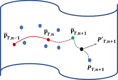
Figure 5: Prediction of next-target subspace. The $(n+1)^{th}$ target subspace $\mathbf{\hat{P}}_{\mathcal{T},n+1}$ (green dot) is an extrapolation of the geodesic from the $(n-1)^{th}$ mean-target subspace $\mathbf{\overline{P}}_{\mathcal{T},n-1}$ to the $n^{th}$ mean-target subspace $\mathbf{\overline{P}}_{\mathcal{T},n}$. The $(n+1)^{th}$ target subspace $\mathbf{P}_{\mathcal{T},n+1}$ can then be compensated to $\mathbf{P^{\prime}}_{\mathcal{T},n+1}$ (black dot).

The principal angle between $\mathbf{\overline{P}}_{\mathcal{T},n-1}$ and $\mathbf{\overline{P}}_{\mathcal{T},n}$ is computed from $\mathbf{\Theta}_{n}\!=\!\arccos{(\mathbf{\Gamma^{\prime}}_{n})}$. Hence, the velocity matrix of the geodesic from $\mathbf{\overline{P}}_{\mathcal{T},n-1}$ to $\mathbf{\overline{P}}_{\mathcal{T},n}$ is as follows:

$$\mathbf{A}_{n}=\mathbf{U^{\prime}}_{2,n}\mathbf{\Theta}_{n}\mathbf{U^{\prime}}_{1,n}^{T}.$$ (16)

The predicted next-target subspace $\mathbf{\hat{P}}_{\mathcal{T},n+1}$ of $(n+1)^{th}$ mini-batch is the subspace obtained by the extrapolation of the geodesic from the $n^{th}$ mean-target subspace $\mathbf{\overline{P}}_{\mathcal{T},n}$ with velocity matrix $\mathbf{A}_{n}$:

$$\mathbf{\hat{P}}_{\mathcal{T},n+1}=\mathbf{Q}_{n}\begin{pmatrix}\mathbf{U^{\prime}}_{1,n}\mathbf{\Gamma^{\prime}}_{n}\\ -\mathbf{U^{\prime}}_{2,n}\mathbf{\Sigma^{\prime}}_{n}\end{pmatrix}.$$ (17)

The procedure of computing the next-target subspace $\mathbf{\hat{P}}_{\mathcal{T},n+1}$ is described in Algorithm 1.

Input:

 $\mathbf{\overline{P}}_{\mathcal{T},n-1}$: Previous mean-target subspace

 $\mathbf{\overline{P}}_{\mathcal{T},n}$:    Current mean-target subspace

Output:

 $\mathbf{\hat{P}}_{\mathcal{T},n+1}$: Prediction of next-target subspace

 

Procedure:

 1) Compute the orthogonal completion $\mathbf{Q}_{n-1}$, $\mathbf{Q}_{n}$ of

  $\mathbf{\overline{P}}_{\mathcal{T},n-1}$, $\mathbf{\overline{P}}_{\mathcal{T},n}$, respectively.

 2) Compute the CS decomposition of $\mathbf{Q}_{n-1}^{T}\mathbf{\overline{P}}_{\mathcal{T},n}$

  by Eq. (15).

 3) Compute the principal angle matrix:

  $\mathbf{\Theta}_{n}=\arccos{(\mathbf{\Gamma^{\prime}}_{n})}$ .

 4) Compute the velocity matrix:

  $\mathbf{A}_{n}=\mathbf{U^{\prime}}_{2,n}\mathbf{\Theta}_{n}\mathbf{U^{\prime}}_{1,n}^{T}$ .

 5) Predict the next-target subspace by Eq. (17) .

Algorithm 1 Prediction of Next-Target Subspace

The predicted next-target subspace $\mathbf{\hat{P}}_{\mathcal{T},n+1}$ is compensated to $\mathbf{P^{\prime}}_{\mathcal{T},n+1}$ as the actual target subspace of $(n+1)^{th}$ mini-batch $\mathbf{P}_{\mathcal{T},n+1}$ arrives. The compensated target subspace $\mathbf{P^{\prime}}_{\mathcal{T},n+1}$ is the introspection of the prediction $\mathbf{\hat{P}}_{\mathcal{T},n+1}$ and the observation $\mathbf{P}_{\mathcal{T},n+1}$.

IV-E Online Domain Adaptation

In this stage, we compute the transformation matrix $\mathbf{G}_{n}$ using the GFK method [2]. The transformation matrix $\mathbf{G}_{n}$ is computed from the source subspace $\mathbf{P}_{\mathcal{S}}$ and the $n^{th}$ mean-target subspace $\mathbf{\overline{P}}_{\mathcal{T},n}$; that is, $\mathbf{G}_{n}=GFK(\mathbf{P}_{\mathcal{S}},\mathbf{\overline{P}}_{\mathcal{T},n})$. After computing the mean-target subspace $\mathbf{\overline{P}}_{\mathcal{T},n}$, we parameterize a geodesic flow from $\mathbf{P}_{\mathcal{S}}$ to $\mathbf{\overline{P}}_{\mathcal{T},n}$ as $\mathbf{\Phi}_{n}:t\in[0,1]\xrightarrow{}\mathbf{\Phi}_{n}(t)\in\mathcal{G}(k,d)$:

$$\mathbf{\Phi}_{n}(t)=\mathbf{P}_{\mathcal{S}}\mathbf{U}_{3,n}\mathbf{\Lambda}_{n}(t)-\mathbf{R}_{\mathcal{S}}\mathbf{U}_{4,n}\mathbf{\Omega}_{n}(t)$$ (18)

under the constraints of $\mathbf{\Phi}_{n}(0)=\mathbf{P}_{\mathcal{S}}$ and $\mathbf{\Phi}_{n}(1)=\mathbf{\overline{P}}_{\mathcal{T},n}$. $\mathbf{R}_{\mathcal{S}}\in\mathbb{R}^{d\times(d-k)}$ denotes the orthogonal complement to $\mathbf{P}_{\mathcal{S}}$; that is, $\mathbf{R}_{\mathcal{S}}^{T}\mathbf{P}_{\mathcal{S}}=\mathbf{0}$. Two orthonormal matrices $\mathbf{U}_{3,n}\in\mathbb{R}^{k\times k}$ and $\mathbf{U}_{4,n}\in\mathbb{R}^{(d-k)\times(d-k)}$ are given by the GSVD[36],

$$\mathbf{Q}_{\mathcal{S}}^{T}\mathbf{\overline{P}}_{\mathcal{T},n}=\begin{pmatrix}\mathbf{U}_{3,n}&\mathbf{0}\\ \mathbf{0}&\mathbf{U}_{4,n}\end{pmatrix}\begin{pmatrix}\mathbf{\Lambda}_{n}(t)\\ \mathbf{-\Omega}_{n}(t)\end{pmatrix}\mathbf{W}_{n}^{T}~{}.$$ (19)

Based on the GFK, the transformation matrix $\mathbf{G}_{n}$ from the target domain to the source domain is found by projecting and integrating over the infinite set of all intermediate subspaces between them:

$$\int_{0}^{1}(\mathbf{\Phi}_{n}(\alpha)^{T}\mathbf{x}_{i})^{T}(\mathbf{\Phi}_{n}(\alpha)^{T}\mathbf{x}_{j})d\alpha=\mathbf{x}_{i}^{T}\mathbf{G}_{n}\mathbf{x}_{j}.$$ (20)

From the above equation, we can derive the closed form of $\mathbf{G}_{n}$ as:

$$\mathbf{G}_{n}=\int_{0}^{1}\mathbf{\Phi}_{n}(\alpha)\mathbf{\Phi}_{n}(\alpha)^{T}d\alpha.$$ (21)

We adopt this $\mathbf{G}_{n}$ as the transformation matrix to the preprocessed target data as $\mathbf{X^{\prime}}_{\mathcal{T},n}=\mathbf{X}^{pre}_{\mathcal{T},n}\mathbf{G}_{n}$, which better aligns the target data to the source domain. $\mathbf{X}^{pre}_{\mathcal{T},n}$ is the target data fed back from the previous mini-batch.

IV-F Cumulative Computation of Transformation Matrix, $\mathbf{G}_{c,n}$

The proposed ICMS method updates the mean-target subspace as each target mini-batch arrives, but the transformation matrix $\mathbf{G}_{n}$ is still computed by merely utilizing the source subspace $\mathbf{P}_{\mathcal{S}}$ and the mean-target subspace $\mathbf{\overline{P}}_{\mathcal{T},n}$. To obtain the transformation matrix that embraces the cumulative temporal dependency, we propose a method of computing the cumulative transformation matrix $\mathbf{G}_{c,n}$. As shown in Fig. 6, we compute the cumulative transformation matrix $\mathbf{G}_{c,n}$ by considering the variation of the mean-target subspaces caused by two consecutive mini-batches. The cumulative transformation matrix $\mathbf{G}_{c,n}$ is computed based on the area bounded by the three points $\mathbf{P}_{\mathcal{S}}$, $\mathbf{\overline{P}}_{\mathcal{T},n-1}$, and $\mathbf{\overline{P}}_{\mathcal{T},n}$ on the manifold. In the OUDA problem, it is assumed that the target domain is shifted continuously but slowly. Hence, the principal angle $\mathbf{\Theta}_{n}(0)$ between the source subspace $\mathbf{P}_{\mathcal{S}}$ and the previous mean-target subspace $\mathbf{\overline{P}}_{\mathcal{T},n-1}$ changes linearly to the principal angle $\mathbf{\Theta}_{n}(1)$ between the source subspace $\mathbf{P}_{\mathcal{S}}$ and the current mean-target subspace $\mathbf{\overline{P}}_{\mathcal{T},n}$. The principal angle between $\mathbf{P}_{\mathcal{S}}$ and the intermediate subspace is denoted as follows:

$$\mathbf{\Theta}_{n}(\beta)=\mathbf{\Theta}_{n}(0)+(\mathbf{\Theta}_{n}(1)-\mathbf{\Theta}_{n}(0))\beta.$$ (22)

To consider all the intermediate subspaces inside the boundary area, double integration is conducted for the computation instead of using Eq. (20):

$$\int_{0}^{1}\int_{0}^{1}(\mathbf{\Phi}_{n}(\alpha,\beta)^{T}\mathbf{x}_{i})^{T}(\mathbf{\Phi}_{n}(\alpha,\beta)^{T}\mathbf{x}_{j})d\alpha d\beta=\mathbf{x}_{i}^{T}\mathbf{G}_{c,n}\mathbf{x}_{j}.$$ (23)

Hence, $\mathbf{G}_{c,n}$ is computed as:

$$\mathbf{G}_{c,n}=\int_{0}^{1}\int_{0}^{1}\mathbf{\Phi}_{n}(\alpha,\beta)\mathbf{\Phi}_{n}(\alpha,\beta)^{T}d\alpha d\beta=\int_{0}^{1}\mathbf{G}_{n}(\beta)d\beta.$$ (24)

Different from the offline domain-adaptation problem [2], the transformation matrix $\mathbf{G}_{n}$ depends on the parameter $\beta$:

$$\mathbf{G}_{n}(\beta)=[\mathbf{P}_{\mathcal{S}}\mathbf{U}_{3,n}\>\>\mathbf{R}_{\mathcal{S}}\mathbf{U}_{4,n}]\begin{bmatrix}\mathbf{\Lambda}_{1,n}(\beta)&\mathbf{\Lambda}_{2,n}(\beta)\\ \mathbf{\Lambda}_{2,n}(\beta)&\mathbf{\Lambda}_{3,n}(\beta)\end{bmatrix}\begin{bmatrix}\mathbf{U}_{3,n}^{T}\mathbf{P}_{\mathcal{S}}^{T}\\ \mathbf{U}_{4,n}^{T}\mathbf{R}_{\mathcal{S}}^{T}\end{bmatrix}.$$ (25)

The computed $\mathbf{G}_{n}(\beta)$ is then integrated over the parameter $\beta$, as shown in the bottom part of Fig. 6. Utilizing the GFK technique [2], the diagonal elements of matrices $\mathbf{\Lambda}_{1,n}(\beta)$, $\mathbf{\Lambda}_{2,n}(\beta)$, and $\mathbf{\Lambda}_{3,n}(\beta)$ are, respectively:

$$\lambda_{1i,n}(\beta) =1+\frac{\sin{2\theta_{i,n}(\beta)}}{2\theta_{i,n}(\beta)},$$

$$\lambda_{2i,n}(\beta) =\frac{\cos{2\theta_{i,n}(\beta)-1}}{2\theta_{i,n}(\beta)},$$

$$\lambda_{3i,n}(\beta) =1-\frac{\sin{2\theta_{i,n}(\beta)}}{2\theta_{i,n}(\beta)}.$$ (26)

Substituting Eq. (25) into Eq. (24), only the second matrix of the right-hand side of Eq. (25) should be integrated with respect to $\beta$. Thus,

$$\mathbf{G}_{c,n}=[\mathbf{P}_{\mathcal{S}}\mathbf{U}_{3,n}\>\>\mathbf{R}_{\mathcal{S}}\mathbf{U}_{4,n}]\begin{bmatrix}\mathbf{\Delta}_{1,n}&\mathbf{\Delta}_{2,n}\\ \mathbf{\Delta}_{2,n}&\mathbf{\Delta}_{3,n}\end{bmatrix}\begin{bmatrix}\mathbf{U}_{3,n}^{T}\mathbf{P}_{\mathcal{S}}^{T}\\ \mathbf{U}_{4,n}^{T}\mathbf{R}_{\mathcal{S}}^{T}\end{bmatrix},$$ (27)

where the diagonal elements of matrices $\mathbf{\Delta}_{1}$, $\mathbf{\Delta}_{2}$, and $\mathbf{\Delta}_{3}$ are, respectively:

$$\delta_{1i,n} =2-\frac{2}{9}\Big{\{}\theta_{i,n}(1)^{2}+\theta_{i,n}(1)\theta_{i,n}(0)+\theta_{i,n}(0)^{2}\Big{\}},$$

$$\delta_{2i,n} =-\frac{1}{2}\Big{\{}\theta_{i,n}(1)+\theta_{i,n}(0)\Big{\}},$$

$$\delta_{3i,n} =\frac{2}{9}\Big{\{}\theta_{i,n}(1)^{2}+\theta_{i,n}(1)\theta_{i,n}(0)+\theta_{i,n}(0)^{2}\Big{\}}.$$ (28)

The computation of the cumulative transformation matrix $\mathbf{G}_{c,n}$ is summarized in Algorithm 2.

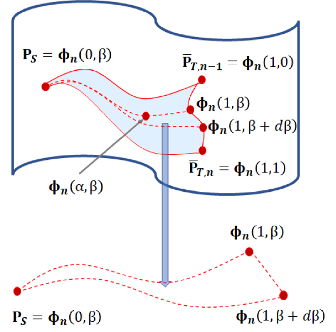
Figure 6: Cumulative computation of transformation matrix $\mathbf{G}_{c,n}$. $\mathbf{G}_{c,n}$ is obtained by integrating over the area bounded by the source subspace $\mathbf{P}_{\mathcal{S}}$, $(n-1)^{th}$ mean-target subspace $\mathbf{\overline{P}}_{\mathcal{T},n-1}$ and $n^{th}$ mean-target subspace $\mathbf{\overline{P}}_{\mathcal{T},n}$ (enclosed and colored area). The subspace inside the area is parameterized as $\mathbf{\Phi}_{n}(\alpha,\beta)$.

Input:

 $\mathbf{P}_{\mathcal{S}}$: Source subspace

 $\mathbf{\overline{P}}_{\mathcal{T},n-1}$: Previous mean-target subspace

 $\mathbf{\overline{P}}_{\mathcal{T},n}$: Current mean-target subspace

Output:

 $\mathbf{G}_{c,n}$: Prediction of next-target subspace

 

Procedure:

 1) Compute the orthogonal completion $\mathbf{Q}_{\mathcal{S}}$, $\mathbf{Q}_{n-1}$,

  $\mathbf{Q}_{n}$ of $\mathbf{P}_{\mathcal{S}}$, $\mathbf{\overline{P}}_{\mathcal{T},n-1}$, $\mathbf{\overline{P}}_{\mathcal{T},n}$, respectively.

 2) Compute the principal angle matrices $\mathbf{\Theta}_{n}(0)$,

  $\mathbf{\Theta}_{n}(1)$.

 3) Compute the cumulative matrix $\mathbf{G}_{c,n}$ by Eq. (27).

Algorithm 2 Cumulative Transformation Matrix $\mathbf{G}_{c,n}$ Computation

IV-G Overall Procedure

The overall procedure of our proposed multi-stage OUDA framework is outlined in Algorithm 3. As shown in Fig. 7, the prediction of the $i^{th}$ target subspace $\mathbf{\hat{P}}_{\mathcal{T},i}$ is computed from the $(i-2)^{th}$ and $(i-1)^{th}$ mean-target subspaces $\mathbf{\overline{P}}_{\mathcal{T},i-2}$ and $\mathbf{\overline{P}}_{\mathcal{T},i-1}$, respectively, whereas the $i^{th}$ cumulative transformation matrix $\mathbf{G}_{c,i}$ is computed from the $(i-1)^{th}$ and $i^{th}$ mean-target subspaces $\mathbf{\overline{P}}_{\mathcal{T},i-1}$ and $\mathbf{\overline{P}}_{\mathcal{T},i}$, respectively.

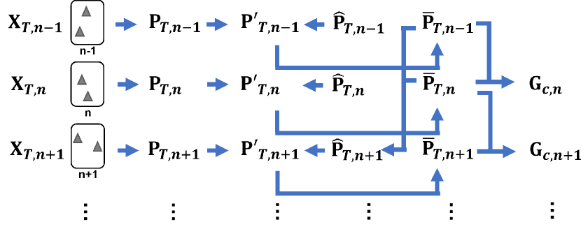
Figure 7: Schematic of subspace prediction and cumulative computation of transformation matrix $\mathbf{G}_{c,n}$.

Input:

 $\mathbf{X}_{\mathcal{S}}$: Source data

 $\mathbf{Y}_{\mathcal{S}}$: Source labels

 $\mathbf{X}_{\mathcal{T},n}$: $n^{th}$ target data mini-batch

 $\mathbf{\overline{P}}_{\mathcal{T},n-1}$: Previous mean-target subspace

Output:

 $\mathbf{\hat{Y}}_{\mathcal{T},n}$: Predicted label of $\mathbf{X}_{\mathcal{T},n}$

 

Procedure:

 1) Compute the subspaces $\mathbf{P}_{\mathcal{S}}$, $\mathbf{P}_{\mathcal{T},n}$, $\mathbf{P}_{\mathcal{T},n-1}$ from

  $\mathbf{X}_{\mathcal{S}}$, $\mathbf{X}_{\mathcal{T},n}$, $\mathbf{X}_{\mathcal{T},n-1}$, respectively.

 2) Predict the target subspace $\mathbf{\hat{P}}_{\mathcal{T},n}$ using

  Algorithm 1.

 3) Compensate the next-target subspace $\mathbf{P^{\prime}}_{\mathcal{T},n}$

  from $\mathbf{\hat{P}}_{\mathcal{T},n}$ and $\mathbf{P}_{\mathcal{T},n}$.

 4) Compute the mean-target subspace $\mathbf{\overline{P}}_{\mathcal{T},n}$ by

  Eq. (7).

 5) Compute $\mathbf{G}_{c,n}$ from $\mathbf{P}_{\mathcal{S}}$, $\mathbf{\overline{P}}_{\mathcal{T},n-1}$, and $\mathbf{\overline{P}}_{\mathcal{T},n}$.

 6) Compute $\mathbf{X^{\prime}}_{\mathcal{T},n}=\mathbf{X}_{\mathcal{T},n}\mathbf{G}_{c,n}$.

 7) Predict the label $\mathbf{\hat{Y}}_{\mathcal{T},n}$ by the classifier trained

  with $\mathbf{X}_{\mathcal{S}}$ and $\mathbf{Y}_{\mathcal{S}}$.

 8) Update the classifier with $\mathbf{X}_{\mathcal{T},n}$ and $\mathbf{\hat{Y}}_{\mathcal{T},n}$.

Algorithm 3 Proposed Multi-stage OUDA Framework

V Experimental Results

We performed extensive computer simulations on five small-scale datasets [7] and one large-scale dataset [38] to validate the performance of our proposed multi-stage OUDA framework in the context of data classification. We first evaluated the major components of the proposed OUDA framework, namely the ICMS technique and the recursive feedback with cumulative computation of the transformation matrix, $\mathbf{G}_{c,n}$, and the next-target subspace prediction. We then verified the effect of adaptive classifier in our proposed framework. We also analyzed how the various factors such as the number of source data $N_{\mathcal{S}}$, the target mini-batch $N_{\mathcal{T}}$, and the dimension of projected subspace $k$ would affect the classification performance. To show the validity of our proposed framework, we illustrated the convergence of our proposed ICMS technique and visualized the projected features. We then validated the performance of our proposed OUDA framework by comparing it to other manifold-based traditional methods in the context of data classification. We selected two existing manifold-based traditional methods for comparisons  –  Evolving Domain Adaptation (EDA) [7] and Continuous Manifold Alignment (CMA) [8]. The CMA method has two variations depending on the domain adaptation techniques –  GFK [2] and Statistical Alignment (SA) [4].

Furthermore, we also conducted experiments on test-time adaptation tasks [31], comparing the performance of our proposed framework with recent Neural-Network-(NN)-based learning models.

V-A Datasets

The six datasets [7] that we have selected are – the Traffic dataset, the Car dataset, the Waveform21 dataset, the Waveform40 dataset, the Weather dataset, and the CIFAR-10-C dataset. These datasets provide a large variety of time-variant images and signals to test upon. The Traffic dataset includes images captured from a fixed traffic camera observing a road over a 2-week period. This dataset consists of 5412 instances of 512-dimensional ($d\!=\!512$) GIST features [39] with two classes as either “heavy traffic” or “light traffic.” The Car dataset contains images of automobiles manufactured between 1950 and 1999 acquired from online databases. This Car dataset includes 1770 instances of 4096-dimensional ($d\!=\!4096$) DeCAF [40] features with two classes as “sedans” or “trucks.” Figure 8(a) depicts example images of sedans or trucks from 1950’s to 1990’s. Figure 8(b) depicts the same road but the scene changes as the environment changes from the morning (left) to afternoon (middle) and night (right). The Waveform21 dataset is composed of 5000 wave instances of 21-dimensional features with three classes. The Waveform40 dataset is the second version of the Waveform21 with additional features. This dataset consists of 40-dimensional features. The Weather dataset includes 18159 daily readings of attributes such as temperature, pressure and wind speed. Those attributes are represented as 8-dimensional features with two classes as “rain” or “no rain.” The CIFAR-10-C dataset is an extension of CIFAR-10 dataset that includes 10 categories of images of 50,000 train images and 10,000 test images. The CIFAR-10 dataset is turned into CIFAR-10-C dataset with 15 types of corruptions at 5 severity levels [38]. The information of these six datasets is summarized in Table II. Dimension of the subspace was assigned as $k=100$ for the datasets of which $d$ is greater than 200, or $k=\frac{d}{2}$ otherwise.

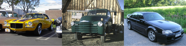
(a)

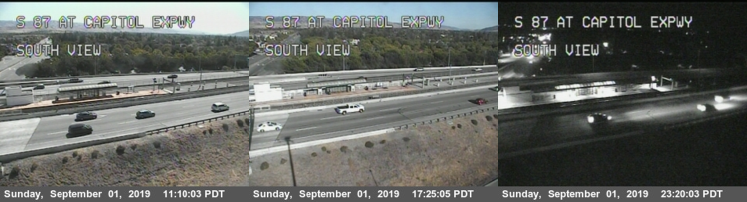
(b)

Figure 8: Image samples of the (a) Car and (b) Traffic datasets.

TABLE II: The table of datasets

Method	Traffic	Car	Wave21	Wave40	Weather	CIFAR-10-C
Number of samples	5412	1770	5000	5000	18159	150000
Dimension of data($d$)	512	4096	21	40	8	-
Default $k$	100	100	10	20	4	100
Number of classes	2	2	3	3	2	10

TABLE III: Average Classification Accuracy (%) and Computation Time (sec) with Various Mean-subspace Computation Methods

	Traffic		Car		Wave21		Wave40		Weather
Method	Accuracy(%)	time(sec)	Accuracy(%)	time(sec)	Accuracy(%)	time(sec)	Accuracy(%)	time(sec)	Accuracy(%)	time(sec)
EDA	69.00	$1.06\times 10^{2}$	82.50	$2.55\times 10^{3}$	72.48	$2.23\times 10^{1}$	66.85	$2.34\times 10^{1}$	69.77	$1.24\times 10^{2}$
Incremental Averaging	68.54	$5.85\times 10^{2}$	85.12	$2.38\times 10^{3}$	82.69	$8.02\times 10^{0}$	80.71	$1.40\times 10^{1}$	69.80	$1.99\times 10^{1}$
Karcher Mean	69.13	$2.62\times 10^{5}$	-	-	82.34	$1.41\times 10^{4}$	80.95	$2.58\times 10^{4}$	68.48	$1.25\times 10^{5}$
ICMS	69.94	$5.75\times 10^{1}$	85.52	$5.50\times 10^{3}$	82.69	$3.19\times 10^{0}$	80.79	$7.58\times 10^{0}$	69.50	$1.62\times 10^{1}$

V-B Analysis of Various Methods on Mean Subspace Computation

One of the characteristics in our proposed OUDA framework is the ICMS technique that computes the mean-target subspace incrementally. In this subsection, we verify that the ICMS technique is the most efficient method for computing the mean-target subspace as compared to the other methods on mean-subspace computation – the incremental averaging and the Karcher mean. The incremental averaging on a subspace simply computes the average matrix $\mathbf{\overline{G}}_{n}$ of $n$ matrices $\mathbf{G}_{i}$ obtained from each target mini-batch as $\mathbf{\overline{G}}_{n}=(1-\frac{1}{n})\mathbf{\overline{G}}_{n-1}+\frac{1}{n}\mathbf{G}_{n}$, where $\mathbf{\overline{G}}_{n-1}$ is the average matrix of previous $(n-1)$ matrices. The Karcher mean is the computation of the mean point of multiple points on a subspace. To validate the computation efficiency of the proposed ICMS technique, we evaluated the computation time of our proposed OUDA framework using the ICMS technique and the next-target subspace prediction as compared to the existing EDA method [7]. We also measured the classification accuracy and the computation time of our proposed framework, replacing the ICMS technique with computation of the incremental averaging or the Karcher mean. The metric for classification accuracy [7] is the average classification accuracy for a set of mini-batches $B$:

$$A(B)=\frac{\sum_{\tau=1}^{|B|}a(\tau)}{|B|},$$ (29)

where $A(B)$ is the average classification accuracy of $|B|$ mini-batches and $a(\tau)$ is the accuracy for the $\tau^{th}$ mini-batch. In this subsection, the feedback stage was not included in our proposed framework since we focused on comparing the methods of mean-subspace computation. Their comparisons of average classification accuracy and computation time on five datasets are shown in Table III.

As shown in Table III, the mean-subspace computation based on the ICMS technique reached the highest average classification accuracy for the Traffic, the Car and the Waveform21 datasets. For the Waveform40 and the Weather datasets, the accuracy with the ICMS computation was less than the accuracy of other methods by $0.19\%$ and $0.43\%$, respectively. Interestingly, the mean-subspace-based methods, not depending on the type of mean-subspace, resulted in comparable or higher average classification accuracy compared to the EDA method. For the Traffic and Weather datasets, the mean-subspace-based methods showed the average classification accuracy at least $68.54\%$ and $68.48\%$, respectively, which were less than the accuracy of the EDA method by $0.66\%$ and $1.85\%$, respectively. In the case of the Car, the Waveform21 and the Waveform40 datasets, the mean-subspace-based methods showed the average classification accuracy at least $85.12\%$, $82.34\%$ and $80.71\%$, which were higher than the accuracy of EDA by $3.18\%$, $13.60\%$ and $20.73\%$, respectively. These results indicated that averaging the subspace leverages the performance of domain adaptation. The incremental averaging might be a reasonable alternative when fast computation is required at the cost of a small dip in recognition performance.

In terms of computation time, our proposed ICMS method was significantly faster than the EDA method and the Karcher-mean computation method for most of the datasets. The reason for this difference on computation time was due to the fact that the Karcher mean was computed in an iterative process. Since the feature dimension of the Car dataset was 4096, which was significantly higher than the feature dimension of the other datasets, the computation time of ICMS was longer than that of the incremental averaging. Especially, the computation time of the Karcher mean computation for the Car dataset was longer than 4 weeks ($2.42\times 10^{6}$ sec) and computational burden was tremendous, which led to tremendous computational burden. These results indicated that our proposed ICMS-based framework is suitable for solving the online data classification problem.

V-C Effect of ICMS with Additional Components

In this subsection, we investigated the performance of the ICMS technique combined with other components in our framework that considers the cumulative temporal dependency among the arriving target data. Coupled with the ICMS technique, we consider the cumulative computation of transformation matrix (Cumulative), the next-target-subspace prediction (NextPred), and recursive feedback (FB) to compensate the arriving target mini-batch $\mathbf{X}_{\mathcal{T},n}$, the target subspace $\mathbf{P}_{\mathcal{T},n+1}$, and the transformation matrix $\mathbf{G}_{n}$ to the pre-aligned target mini-batch $\mathbf{X}^{pre}_{\mathcal{T},n}$, the next-target-subspace prediction $\mathbf{P^{\prime}}_{\mathcal{T},n+1}$, and the cumulative transformation matrix $\mathbf{G}_{c,n}$, respectively. The NextPred component is suitable for noisy target domain, whereas the Cumulative component is beneficial for gradually evolving target domain. Hence, it is not desirable to include both the NextPred component and the Cumulative component (i.e. ICMS + FB + NextPred + Cumul) in our proposed framework. We thus selected three recursive feedback variants to combine with the ICMS technique:

1. ICMS + Cumulative  –   ICMS computation and cumulative computation of the transformation matrix $\mathbf{G}_{c,n}$;

2. ICMS + NextPred  –   ICMS computation and the next-target-subspace prediction;

3. ICMS + FB+ NextPred  –   ICMS computation and the next-target-subspace prediction with recursive feedback.

TABLE IV: Average Classification Accuracy $A(B)$ (%) of the ICMS Method with Recursive Feedback

Method	Traffic	Car	Wave21	Wave40	Weather
ICMS+Cumulative	71.19	82.5	81.66	81.54	69.5
ICMS+FB+NextPred	69.28	83.78	81.9	82.02	69.48
ICMS+NextPred	68.54	85.93	83.45	81.43	70.63

We then compared the average classification accuracy on these three variants of recursive feedback combined with the ICMS technique. Since the average classification accuracy depends on the feature dimension $k$, we plotted the classification results versus the subspace dimension $k$ as shown in Fig. 9, varying from $5\%$ to $50\%$ of the data dimension $d$. For the Waveform40 dataset (see Fig. 9(a)), the average classification accuracy of (ICMS + FB + NextPred) outperformed that of other variants as the value of $k$ increased. When the value of $k$ was small, the average classification accuracy of (ICMS + Cumulative) was the highest among other variants. This result indicated that the effect of recursive feedback on the average classification accuracy is marginal when $k$ is small.

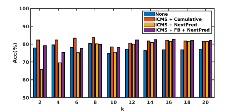
(a) Waveform40 dataset.

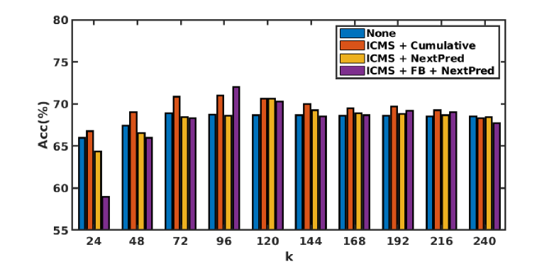
(b) Traffic dataset.

Figure 9: Effects of averaging target subspace and recursive feedback on the Waveform40 and the Traffic datasets.

TABLE V: Corruption Error (%) on Noisy CIFAR-10-C dataset

Method	gauss	shot	impul	defoc	glass	motn	zoom	snow	frost	fog	brit	contr	elast	pixel	jpeg	average
ICMS [11]	31.73	27.91	42.29	19.91	39.09	21.62	19.20	23.53	25.52	20.60	12.77	22.12	31.92	23.54	30.93	26.18
ICMS + FB	31.94	28.89	40.95	18.92	40.39	21.04	16.56	22.77	23.54	19.16	13.11	20.31	29.53	23.03	30.47	25.37
ICMS + NextPred	32.42	28.90	39.41	17.60	40.62	21.36	16.78	21.56	24.08	19.04	14.42	19.26	30.00	23.63	31.44	25.37
ICMS + FB + NextPred	31.60	28.81	38.78	18.26	40.20	19.53	16.87	22.35	24.00	18.62	14.61	21.19	28.28	22.86	31.75	25.18

TABLE VI: Corruption Error (%) on CIFAR-10-C Dataset with Gradually Changing Severity Level.

Method	Group	Severity Level	gauss	shot	impul	defoc	glass	motn	zoom	snow	frost	fog	brit	contr	elast	pixel	jpeg	average
ICMS [11]	1	1,2,3,4,5	27.02	24.1	36.16	13.43	35.46	15.59	13.03	17.84	19.39	15.08	9.16	15.67	25.86	19.53	26.43	20.92
ICMS + Cumul	1	1,2,3,4,5	24.94	22.64	33.89	12.03	33.63	13.86	11.29	15.93	17.61	13.41	8.25	13.78	23.68	17.71	24.12	19.12
ICMS [11]	2	1, 3, 5	29.78	27.36	39.49	16.16	38.89	18.62	17.37	18.03	23.53	15.65	9.95	19.33	30.84	19.72	27.53	23.48
ICMS + Cumul	2	1, 3, 5	29.05	24.15	38.44	15.61	35.69	18.79	13.23	21.62	20.71	18.03	10.59	14.50	25.45	20.91	27.28	22.27

TABLE VII: Corruption Error (%) on CIFAR-10-C dataset for non-NN-based methods (severity level 5).

Method	Classifier	gauss	shot	impul	defoc	glass	motn	zoom	snow	frost	fog	brit	contr	elast	pixel	jpeg	average
Source (No Adaptation)	NN	72.33	65.7	72.9	46.9	54.3	34.8	42.0	25.1	41.3	26.0	9.3	46.7	26.6	58.5	30.3	43.51
First Target	SVM	29.50	28.71	39.00	18.49	39.63	18.42	16.71	21.42	22.00	19.39	12.37	17.69	29.27	21.62	29.94	24.28
ICMS-SVM	SVM	26.95	24.04	36.07	13.46	35.47	15.40	12.89	17.78	19.21	14.98	9.18	15.56	25.67	19.46	26.38	20.83

For the Traffic dataset (see Fig. 9(b)), the average classification accuracy of (ICMS + Cumulative) was higher than that of other variants for most $k$ values. However, the average classification accuracy of (ICMS + FB + NextPred) was the highest for $k=96$, and this accuracy was the highest among the accuracies of all the variants. This result showed that recursive feedback significantly leverages the classification performance with proper subspace dimension $k$.

Table IV showed the average classification accuracy for the ICMS method coupled with 3 recursive feedback variants of our proposed framework when the values of subspace dimension $k$ were set to the default values in Table II. For the Traffic dataset, the average classification accuracy of (ICMS + Cumulative) was the highest among the 3 variants of our proposed framework. This result was shown in Fig. 9(b), where the average classification accuracy of (ICMS + FB + NextPred) decreased after the value of $k=96$. The average classification accuracy of (ICMS + NextPred) was the highest ($71.19\%$) for the Waveform40 dataset. This result was shown in Fig. 9(a) for $k=20$.

For the Car, Wave21, and Weather datasets, the average classification accuracies of (ICMS + FB + NextPred) were lower than that of (ICMS + NextPred). The reason for these results is that adjacent target mini-batches lacked strong temporal dependency (the Car dataset) and the subspace dimension $k$ was too small (the Wave21 and Weather datasets). Hence, we concluded that the recursive feedback stage improves the classification accuracy when the subspace dimension is large enough and the target mini-batches have strong temporal dependency.

V-D Effect of Next-Target-Subspace Prediction and Recursive Feedback

In this subsection, we demonstrated the effect of next-target-subspace prediction and recursive feedback in our proposed framework. To verify the robustness of subspace prediction and recursive feedback, we measured the corruption errors on four variants for comparison – ICMS, ICMS + FB, ICMS + NextPred, ICMS + FB + NextPred. To conduct experiments on a large-scale dataset with noisy domain, we blended several corruption levels of images in CIFAR-10-C dataset. Specifically, we replaced 20% of the target images of corruption level 5 with corruption level 1. As shown in Table V, the errors of (ICMS + FB) and (ICMS + NextPred) showed lower corruption errors than ICMS [11], and the error of (ICMS + FB + NextPred) was the lowest among all the variants. From these results, we concluded that subspace prediction and recursive feedback stages increase the robustness of our OUDA framework when the target subspaces are noisy.

V-E Effect of Cumulative Computation of Transformation Matrix

Transformation matrix computed by our proposed framework aligns target data closer to the source domain. Especially, the transformation matrix obtained by cumulative computation showed significant improvement for gradually evolving target domains. To validate the effectiveness of cumulative computation, we measured the classification error of images in CIFAR-10-C dataset, changing the corruption level from 1 to 5. To compare the results on different evolving velocity of the target domain, we set the increment of corruption level as 1 for one group and 2 for another. As shown in Table VI, the cumulative computation of transformation matrix component lowered the corruption error from 20.92% to 19.12% and 23.48% to 22.27% in group 1 and group 2, respectively. From these results, we concluded that cumulative computation of transformation matrix is effective when the source and the first target is similar and the target domain is gradually changing.

V-F Classifier Update for Non-Neural-Network-Based Methods

In this subsection, we verified the effect of non-NN-based adaptive classifier on our proposed framework. For fair comparisons, we measured the average classification accuracy of variants of our framework (described in Section V-C) with and without classifier adaptation. The number of source data was 10% of the number of entire data sample and the batch-size of the target data was $N_{\mathcal{T}}=2$. The classifier was updated by each target mini-batch with predicted pseudo-labels. Tables VIII and IX showed the average classification accuracy of our framework for the Traffic and the Weather datasets, respectively. For all the variants of our proposed ICMS method, the classification accuracy of adaptive classifier was higher, from 0.21% to 3.88%, than that of the source classifier. These results showed that the adaptive classifier leveraged the performance of our proposed framework.

Table VII showed the effect of adaptive SVM classifier for the CIFAR-10-C dataset. Our method (ICMS-SVM) improved the test-time adaptation compared to the classifier trained on the first target mini-batch. For all the corruption types, errors of the ICMS-SVM method were lower than that of the first target, from 7.51% to 27.20%. These results showed that the ICMS technique improves the online adaptation for large-scale datasets.

TABLE VIII: Average Classification Accuracy $A(B)$ (%) of the ICMS Method with Adaptive Classifier on Traffic Dataset

Method	Fixed Classifier	Adaptive Classifier
ICMS + NextPred	67.89	70.63
ICMS + Cumulative	69.77	71.63
ICMS + FB + NextPred	70.63	71.44

TABLE IX: Average Classification Accuracy $A(B)$ (%) of the ICMS Method with Adaptive Classifier on Weather Dataset

Method	Fixed Classifier	Adaptive Classifier
ICMS + NextPred	71.68	72.09
ICMS + Cumulative	72.07	72.24
ICMS + FB + NextPred	71.89	72.04

V-G Online Classification Accuracy of Proposed Framework

To further understand the characteristics of our proposed OUDA framework for online classification performance, we investigated the effect of each stage toward the performance of proposed framework. For consistency, we selected the same ICMS method combined with 3 recursive feedback variants as in the previous subsection. In addition to the average accuracy $A(B)$ metric, we also compared the classification accuracy as each target mini-batch arrived by plotting $a(\tau)$ versus the number of mini-batches $|B|$ (see Fig. 10). Figure 10 indicated that our proposed framework and its variants outperformed the EDA method for most of the datasets. In Fig. 10(a), a sudden drift occurred from the $100^{th}$ mini-batch to the $900^{th}$ mini-batch, which resulted in an abrupt decrease of the accuracy. After the $900^{th}$ mini-batch, the accuracy was recovered as the number of arriving mini-batch increased. For the Car dataset, the average accuracy was slightly decreased since the target data were evolving in a long time-horizon (i.e., from 1950 to 1999), which resulted in more discrepancies between the source and the target domains. In terms of the gap between the highest and the lowest accuracies, the Traffic and Waveform40 datasets showed more gap (15% to 25%) compared to other datasets (5% to 10%). We concluded that the computation of transformation matrix (Cumulative) and recursive feedback (FB) showed more significant effect for dynamic datasets.

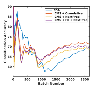
(a) Traffic dataset

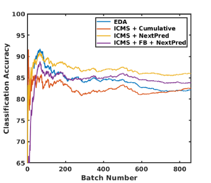
(b) Car dataset

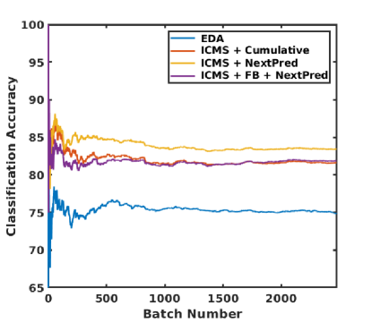
(c) Waveform21 dataset

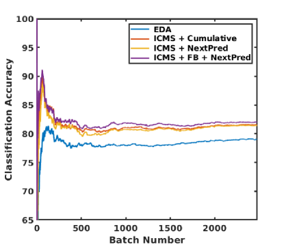
(d) Waveform40 dataset

Figure 10: Classification accuracy of each mini-batch $a(\tau)$ (%) computed by the baseline and variants of the proposed framework.

V-H Convergence of Computed Mean-target Subspace

In this subsection, we empirically demonstrated the convergence of mean-target subspace computed by the ICMS technique. To prove that the mean-target subspace converges to a fixed subspace, we computed and plotted the geodesic distance between the source subspace $\mathbf{P}_{\mathcal{S}}$ and the mean-target subspace $\mathbf{\overline{P}}_{\mathcal{T},n}$ (i.e., $d(\mathbf{P}_{\mathcal{S}},\mathbf{\overline{P}}_{\mathcal{T},n})$). Furthermore, we observed the stability of ICMS technique by showing that the geodesic distance [41] between two consecutive mean-target subspaces $\mathbf{\overline{P}}_{\mathcal{T},n-1}$ and $\mathbf{\overline{P}}_{\mathcal{T},n}$ (i.e., $d(\mathbf{\overline{P}}_{\mathcal{T},n-1},\mathbf{\overline{P}}_{\mathcal{T},n})$) converged to zero as the number of arriving target mini-batches increased. Figures 11(a) and 11(c) showed the geodesic distances between the source subspace $\mathbf{P}_{\mathcal{S}}$ and the mean-target subspace $\mathbf{\overline{P}}_{\mathcal{T},n}$ for the Waveform21 and the Car datasets, respectively. Their geodesic distances converged to a constant. Similarly, Figures 11(b) and 11(d) showed the geodesic distances between the two consecutive mean-target subspaces $\mathbf{\overline{P}}_{\mathcal{T},n-1}$ and $\mathbf{\overline{P}}_{\mathcal{T},n}$ for the Waveform21 and the Car datasets, respectively. These geodesic distances converged to zero. Thus, the convergence of the above geodesic distances validated the proposed ICMS technique for computing the mean-target subspace.

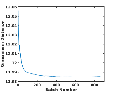
(a) $d(\mathbf{P}_{\mathcal{S}},\mathbf{\overline{P}}_{\mathcal{T},n})$

(b) $d(\mathbf{\overline{P}}_{\mathcal{T},n-1},\mathbf{\overline{P}}_{\mathcal{T},n})$

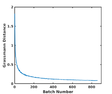
(c) $d(\mathbf{P}_{\mathcal{S}},\mathbf{\overline{P}}_{\mathcal{T},n})$

(d) $d(\mathbf{\overline{P}}_{\mathcal{T},n-1},\mathbf{\overline{P}}_{\mathcal{T},n})$

Figure 11: Geodesic distances between two subspaces. Figures (a) and (b) used the Waveform21 dataset. Figures (c) and (d) used the Car dataset.

V-I Parameter Sensitivity

We also visualized the effect of both parameters $k$ and $N_{\mathcal{T}}$ by measuring the accuracy corresponding to their various values. Figures 12(a) showed that the classification accuracy significantly depended on the value of $k$ while it remained relatively stable with the values of $N_{\mathcal{T}}$. From Fig. 12(b), the classification accuracy was the highest when $k$ and $N_{\mathcal{T}}$ were small, but the difference between the highest and the lowest accuracies was $4.5\%$, which was relatively negligible compared to Fig. 12(a).

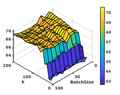
(a)

(b)

Figure 12: Sensitivity analysis on $k$ and batchsize on (a) Traffic (b) Car dataset.

V-J Comparison with Existing Manifold-based Traditional Methods

We compared the average classification accuracy of the proposed OUDA framework with two existing manifold-based traditional methods – Evolving Domain Adaptation (EDA) [7] and Continuous Manifold Alignment (CMA) [8]. The CMA method has two variations depending on the domain adaptation techniques –  GFK [2] and SA [4]. Among the variants of our proposed OUDA framework, we selected the (ICMS + FB + NextPred) variant for comparison with EDA and CMA methods. This (ICMS + FB + NextPred) variant uniquely shows major contributions of the ICMS technique combined with recursive feedback in our proposed framework. In the comparison, we assigned the parameter values of the (ICMS + FB + NextPred) variant the same as those of EDA and CMA methods. The batch-size of the arriving target data was $N_{\mathcal{T}}=2$. Except for the EDA method that adopted the Incremental Semi-Supervised Learning (ISSL) technique for classifying the unlabeled target data, all other approaches adopted the basic Support-Vector-Machine [42] classifiers for target-label prediction.

The results of comparison on the five datasets are shown in Table X. In Table X, our proposed OUDA framework obtained a higher average classification accuracy than traditional methods (i.e., CMA+GFK, CMA+SA, and EDA methods) for all the five datasets. For these five datasets, the highest average classification accuracy among the traditional methods were $69.00\%$, $82.73\%$, $74.65\%$, $79.66\%$, $64.79\%$. The average classification accuracy of our proposed OUDA framework for the respective five datasets were $69.28\%$, $83.78\%$, $81.9\%$, $82.02\%$, and $69.48\%$. This result demonstrated that our proposed OUDA framework outperformed the other traditional methods on the data classification problem for all the datasets.

TABLE X: Overall Accuracy $A(B)$ (%) of the Traditional Methods and the Proposed OUDA Framework

Method	Traffic	Car	Wave21	Wave40	Weather
CMA+SA	41.33	56.45	33.84	33.05	31.40
CMA+GFK [7, 8]	68.87	82.73	69.15	68.77	63.81
EDA [7]	69.00	82.59	74.65	79.66	64.79
Proposed Framework	69.28	83.78	81.9	82.02	69.48

V-K Comparison with Neural-Network-based Methods

We compared the corruption error (%) with several NN-based-online-adaptation methods – classifier with no adaptation with target data (Source), Test Entropy Minimization (Tent) [31], and Test-Time Normalization (BN) [30]. To utilize our framework on test-time adaptation tasks, we first extracted the features before the classifier module of NN. Our proposed framework then transforms these features and input the transformed features through the classifier. Since the source data are not accessible in test-time adaptation tasks, our framework aligns the arriving target data to the initial target domain instead of the source domain. For the experiments on corruption, we used Wide Residual Network with 28 layers (WRN-28-10) [43] and Residual Network with 26 layers (ResNet26) [44] on the CIFAR-10-C dataset. Dimensions of the features extracted from WRN-28-10 and ResNet26 were 640 and 256, respectively. These extracted features were transformed by our proposed framework. We optimized the parameters of WRN-28-10 with Adam optimizer [45], where the batchsize and learning rate were 200 and 0.001, respectively. For ResNet26, the batchsize and learning rate were 128 and 0.001, respectively. The classification errors for various types of corruption are shown in Table XI.

For both WRN-28-10 and ResNet26, our ICMS-NN showed the lowest error among the NN-based methods. For WRN-28-10 and ResNet26, the corruption errors of ICMS-NN were 18.24% and 14.1%, respectively. In terms of the difference of errors, our ICMS was more effective for non-NN models than NN models. This is due to the characteristic of ICMS, which computes the transformation matrix based on the GFK technique. However, the errors of NN-based methods (BN, Tent, and ICMS-NN) were lower than the non-NN-based methods (First Target, ICMS-SVM) for most of the corruption types, which indicate that the NN-based models adapted with target data better than the non-NN-based models. These results showed that our proposed framework leverages the test-time-adaptation task for both NN-based and non-NN-based models.

TABLE XI: Average Corruption Error (%) on CIRAR-10-C Dataset for NN-based Methods (severity level 5)

Method	WRN-28-10	ResNet26
Source	43.51	40.8
BN [30]	20.4	17.3
Tent [31]	18.59	14.3
ICMS-NN	18.24	14.1

VI Conclusion and Future Work

We have proposed a multi-stage framework for tackling the OUDA problem, which includes a novel technique of incrementally computing the mean-target subspace on a Grassmann manifold. We have proved that the mean-target subspace computed by the ICMS method is a valid close approximation to the Karcher mean with efficient computation time. To achieve more robust online domain adaptation, we proposed to utilize subspace prediction and cumulative computation of transformation matrix by considering the flow of target subspaces on the Grassmann manifold. We also verified that the adaptive classifier improves the performance of online adaptation. Extensive experiments on various datasets demonstrated that our proposed OUDA framework outperforms existing traditional manifold-based methods and NN-based learning methods in terms of classification performance and computation time. Moreover, contribution of each stage in our proposed framework has been analyzed by comparing the variants of our proposed method with or without each stage. Future work includes extension of the proposed ICMS technique and the OUDA framework to more challenging domain adaptation applications.

Jihoon Moon received the B.S. and M.S. degrees in Electrical and Computer Engineering from the Seoul National University, South Korea, in 2013 and 2015, respectively. His current research focuses on online domain adaptation, computer vision and robotics. Currently he is pursuing the Ph.D. degree at the Elmore Family School of Electrical and Computer Engineering, Purdue University, West Lafayette, Indiana, U.S.A.

Debasmit Das (S’11-M’21) received the B.Tech. degree in Electrical Engineering from the Indian Institute of Technology, Roorkee in 2014 and the Ph.D. degree from the School of Electrical and Computer Engineering, Purdue University, West Lafayette, Indiana in 2020. He is currently a Senior Machine Learning Researcher at Qualcomm AI Research, Qualcomm Technologies, Inc., San Diego, CA, investigating efficient and personalized learning solutions. He is an associate editor of Wiley Applied AI Letters and he also regularly reviews machine learning articles for IEEE, ACM, Springer and Elesevier journals.

C. S. George Lee (S’71–M’78–SM’86–F’93) is a Professor of Electrical and Computer Engineering at Purdue University, West Lafayette, Indiana. His current research focuses on transfer learning and skill learning, human-centered robotics, and neuro-fuzzy systems. In addition to publishing extensively in those areas, he has co-authored two graduate textbooks, Robotics: Control, Sensing, Vision, and Intelligence (McGraw-Hill, 1986) and Neural Fuzzy Systems: A Neuro-Fuzzy Synergism to Intelligent Systems (Prentice-Hall, 1996). Dr. Lee is an IEEE Fellow, a recipient of the IEEE Third Millennium Medal Award, the Saridis Leadership Award and the Distinguished Service Award from the IEEE Robotics and Automation Society. Dr. Lee received the Ph.D. degree from Purdue University, West Lafayette, Indiana, and the M.S.E.E. and B.S.E.E. degrees from Washington State University, Pullman, Washington.

References

- [1] V. M. Patel, R. Gopalan, R. Li, and R. Chellappa, “Visual domain adaptation: A survey of recent advances,” IEEE Signal Process. Mag., vol. 32, no. 3, pp. 53–69, 2015.
- [2] B. Gong, Y. Shi, F. Sha, and K. Grauman, “Geodesic flow kernel for unsupervised domain adaptation,” in IEEE Conf. Comput. Vis. Pattern Recog. (CVPR), 2012, pp. 2066–2073.
- [3] J. Zhang, W. Li, and P. Ogunbona, “Joint geometrical and statistical alignment for visual domain adaptation,” in Proc. IEEE Conf. Comput. Vis. Pattern Recog. (CVPR), 2017, pp. 1859–1867.
- [4] B. Fernando, A. Habrard, M. Sebban, and T. Tuytelaars, “Unsupervised visual domain adaptation using subspace alignment,” in Proc. IEEE Int. Conf. Comput. Vis. (ICCV), 2013, pp. 2960–2967.
- [5] S. Vascon, S. Aslan, A. Torcinovich, T. van Laarhoven, E. Marchiori, and M. Pelillo, “Unsupervised domain adaptation using graph transduction games,” in Int. J. Conf. on Neural Networks (IJCNN). IEEE, 2019, pp. 1–8.
- [6] A. Gaidon and E. Vig, “Online domain adaptation for multi-object tracking,” arXiv preprint arXiv:1508.00776, 2015.
- [7] A. Bitarafan, M. S. Baghshah, and M. Gheisari, “Incremental evolving domain adaptation,” IEEE Trans. Knowl. Data Eng. (TKDE), vol. 28, no. 8, pp. 2128–2141, 2016.
- [8] J. Hoffman, T. Darrell, and K. Saenko, “Continuous manifold based adaptation for evolving visual domains,” in Proc. IEEE Conf. Comput. Vis. Pattern Recog. (CVPR), 2014, pp. 867–874.
- [9] A. Kumar, T. Ma, and P. Liang, “Understanding self-training for gradual domain adaptation,” in Int. Conf. Mach. Learn. (ICML). PMLR, 2020, pp. 5468–5479.
- [10] A. Bobu, E. Tzeng, J. Hoffman, and T. Darrell, “Adapting to continuously shifting domains,” 2018.
- [11] J. Moon, D. Das, and C. G. Lee, “Multi-step online unsupervised domain adaptation,” in Proc. IEEE Int. Conf. Acoust. Speech Signal Process. (ICASSP), 2020, pp. 41 172–41 576.
- [12] H. Karcher, “Riemannian center of mass and mollifier smoothing,” Commun. Pure Appl. Math., vol. 30, no. 5, pp. 509–541, 1977.
- [13] M. Long, Y. Cao, J. Wang, and M. Jordan, “Learning transferable features with deep adaptation networks,” in Int. Conf. Mach. Learn. (ICML). PMLR, 2015, pp. 97–105.
- [14] A. Berlinet and C. Thomas-Agnan, Reproducing kernel Hilbert spaces in probability and statistics. Springer Science & Business Media, 2011.
- [15] B. Sun, J. Feng, and K. Saenko, “Return of frustratingly easy domain adaptation,” in Proc. AAAI. Conf. Artificial Intelligence, vol. 30, no. 1, 2016.
- [16] J. Wang, W. Feng, Y. Chen, H. Yu, M. Huang, and P. S. Yu, “Visual domain adaptation with manifold embedded distribution alignment,” in Proc. ACM. Int. Conf. Multimedia, 2018, pp. 402–410.
- [17] J. F. Nash et al., “Equilibrium points in n-person games,” Proc. National Academy of Sciences, vol. 36, no. 1, pp. 48–49, 1950.
- [18] M. Wulfmeier, A. Bewley, and I. Posner, “Addressing appearance change in outdoor robotics with adversarial domain adaptation,” in Proc. IEEE/RSJ Int. Conf. Intell. Robot. Syst. (IROS), 2017, pp. 1551–1558.
- [19] I. Goodfellow, J. Pouget-Abadie, M. Mirza, B. Xu, D. Warde-Farley, S. Ozair, A. Courville, and Y. Bengio, “Generative adversarial nets,” in Advan. Neu. Inf. Proc. Syst. (NIPS), 2014, pp. 2672–2680.
- [20] M. Wulfmeier, A. Bewley, and I. Posner, “Incremental adversarial domain adaptation for continually changing environments,” in Proc. IEEE Int. Conf. Robot. Autom. (ICRA), 2018, pp. 1–9.
- [21] X.-Q. Zeng and G.-Z. Li, “Incremental partial least squares analysis of big streaming data,” Pattern Recognit., vol. 47, no. 11, pp. 3726–3735, 2014.
- [22] H. Liu, M. Long, J. Wang, and Y. Wang, “Learning to adapt to evolving domains.” in Advan. Neu. Inf. Proc. Syst. (NIPS), 2020.
- [23] C. Finn, P. Abbeel, and S. Levine, “Model-agnostic meta-learning for fast adaptation of deep networks,” in Int. Conf. Mach. Learn. (ICML). PMLR, 2017, pp. 1126–1135.
- [24] M. Mancini, H. Karaoguz, E. Ricci, P. Jensfelt, and B. Caputo, “Kitting in the wild through online domain adaptation,” in Proc. IEEE/RSJ Int. Conf. Intell. Robot. Syst. (IROS), 2018, pp. 1103–1109.
- [25] S. Ioffe and C. Szegedy, “Batch normalization: Accelerating deep network training by reducing internal covariate shift,” in Int. Conf. Mach. Learn. (ICML). PMLR, 2015, pp. 448–456.
- [26] Z. Wu, X. Wang, J. E. Gonzalez, T. Goldstein, and L. S. Davis, “Ace: Adapting to changing environments for semantic segmentation,” in IEEE Conf. Comput. Vis. Pattern Recog. (CVPR), 2019, pp. 2121–2130.
- [27] J. Xu, D. Vázquez, K. Mikolajczyk, and A. M. López, “Hierarchical online domain adaptation of deformable part-based models,” in Proc. IEEE Int. Conf. Robot. Autom. (ICRA). IEEE, 2016, pp. 5536–5541.
- [28] R. Wu, C. Guo, Y. Su, and K. Q. Weinberger, “Online adaptation to label distribution shift,” Advan. Neu. Inf. Proc. Syst. (NIPS), vol. 34, 2021.
- [29] Y. Sun, X. Wang, Z. Liu, J. Miller, A. Efros, and M. Hardt, “Test-time training with self-supervision for generalization under distribution shifts,” in Int. Conf. Mach. Learn. (ICML). PMLR, 2020, pp. 9229–9248.
- [30] S. Schneider, E. Rusak, L. Eck, O. Bringmann, W. Brendel, and M. Bethge, “Improving robustness against common corruptions by covariate shift adaptation,” Advan. Neu. Inf. Proc. Syst. (NIPS), vol. 33, pp. 11 539–11 551, 2020.
- [31] D. Wang, E. Shelhamer, S. Liu, B. A. Olshausen, and T. Darrell, “Tent: Fully test-time adaptation by entropy minimization,” in Int. Conf. Learn. Repr. (ICLR), 2021.
- [32] A. Edelman, T. A. Arias, and S. T. Smith, “The geometry of algorithms with orthogonality constraints,” SIAM J. Matrix Anal. Appl., vol. 20, no. 2, pp. 303–353, 1998.
- [33] I. M. James, The topology of Stiefel manifolds. Cambridge University Press, 1976, vol. 24.
- [34] S. Wold, K. Esbensen, and P. Geladi, “Principal component analysis,” Chemom. Intell. Lab. Syst., vol. 2, no. 1-3, pp. 37–52, 1987.
- [35] K. A. Gallivan, A. Srivastava, X. Liu, and P. Van Dooren, “Efficient algorithms for inferences on grassmann manifolds,” in IEEE Stat. Signal Process. Workshop SSP, 2003, pp. 315–318.
- [36] C. C. Paige and M. A. Saunders, “Towards a generalized singular value decomposition,” SIAM J. Numer. Anal, vol. 18, no. 3, pp. 398–405, 1981.
- [37] R. Gopalan, R. Li, and R. Chellappa, “Domain adaptation for object recognition: An unsupervised approach,” in Proc. IEEE Int. Conf. Comput. Vis. (ICCV), 2011, pp. 999–1006.
- [38] D. Hendrycks and T. Dietterich, “Benchmarking neural network robustness to common corruptions and perturbations,” arXiv preprint arXiv:1903.12261, 2019.
- [39] A. Oliva and A. Torralba, “Modeling the shape of the scene: A holistic representation of the spatial envelope,” International journal of computer vision, vol. 42, no. 3, pp. 145–175, 2001.
- [40] J. Donahue, Y. Jia, O. Vinyals, J. Hoffman, N. Zhang, E. Tzeng, and T. Darrell, “Decaf: A deep convolutional activation feature for generic visual recognition,” in International conference on machine learning. PMLR, 2014, pp. 647–655.
- [41] J. Hamm and D. D. Lee, “Grassmann discriminant analysis: a unifying view on subspace-based learning,” in Int. Conf. Mach. Learn. (ICML). ACM, 2008, pp. 376–383.
- [42] J. A. Suykens and J. Vandewalle, “Least squares support vector machine classifiers,” Neural Process. Lett., vol. 9, no. 3, pp. 293–300, 1999.
- [43] S. Zagoruyko and N. Komodakis, “Wide residual networks,” in Proceedings of the British Machine Vision Conference (BMVC). BMVA Press, September 2016, pp. 87.1–87.12.
- [44] K. He, X. Zhang, S. Ren, and J. Sun, “Deep residual learning for image recognition,” in Proceedings of the IEEE conference on computer vision and pattern recognition, 2016, pp. 770–778.
- [45] D. P. Kingma and J. Ba, “Adam: A method for stochastic optimization,” in 3rd International Conference on Learning Representations, ICLR 2015, San Diego, CA, USA, May 7-9, 2015, Conference Track Proceedings, Y. Bengio and Y. LeCun, Eds., 2015.