AnoShift: A Distribution Shift Benchmark for Unsupervised Anomaly Detection

Abstract

Analyzing the distribution shift of data is a growing research direction in nowadays Machine Learning (ML), leading to emerging new benchmarks that focus on providing a suitable scenario for studying the generalization properties of ML models. The existing benchmarks are focused on supervised learning, and to the best of our knowledge, there is none for unsupervised learning. Therefore, we introduce an unsupervised anomaly detection benchmark with data that shifts over time, built over Kyoto-2006+, a traffic dataset for network intrusion detection. This type of data meets the premise of shifting the input distribution: it covers a large time span ($10$ years), with naturally occurring changes over time (e.g. users modifying their behavior patterns, and software updates). We first highlight the non-stationary nature of the data, using a basic per-feature analysis, t-SNE, and an Optimal Transport approach for measuring the overall distribution distances between years. Next, we propose AnoShift, a protocol splitting the data in IID, NEAR, and FAR testing splits. We validate the performance degradation over time with diverse models, ranging from classical approaches to deep learning. Finally, we show that by acknowledging the distribution shift problem and properly addressing it, the performance can be improved compared to the classical training which assumes independent and identically distributed data (on average, by up to $3\%$ for our approach). Dataset and code are available at https://github.com/bit-ml/AnoShift/.

1 Introduction

Analyzing and developing Machine Learning algorithms under gradual distribution shifts is a problem of high interest in the research community. There is a growing enthusiasm for building benchmarks over existing or new datasets [26, 22, 44, 6, 20], that formulate a setup for isolating the shifting aspect and create a better ground for this research field. A better understanding of the distribution shift problem might lead to findings of underlying fundamental aspects, shedding new light on robustness and generalization problems. We argue that the distribution shift occurs naturally and gradually in a continuous data stream (e.g. monitoring network traffic), allowing an in-depth analysis of the problem. On the other side, artificially generated scenarios usually exhibit sudden changes that do not simulate the natural shift problem. Yet, the annotation process for streaming data is quite difficult and expensive, considering the massive amount of data.

From a practical point of view, continuous IT infrastructure monitoring has become essential for computer security and resilience. Recent anomaly detection and intrusion detection systems (IDS) obtain strong results on specific datasets but drastically fail in real-world scenarios [47]. Our experimental analysis proved a natural change of the Kyoto-2006+ data over the $10$ years period when the data was collected. The shift is noticeable both over the input distribution and considering the performance of several anomaly detection systems. Several reasons behind the observed shift are: users leaving or coming to the network, per user interest changes leading to network interaction changes, updates to the software versions, patching old vulnerabilities but revealing new attack vectors for intruders.

Figure 1: a) The proposed AnoShift splits over Kyoto-2006+ dataset. The IID (gray) testing split comes from the same temporal span as the TRAIN set (white), while NEAR (yellow) and FAR (blue) splits are from different time spans, with NEAR being closer to the training set than FAR. b) To highlight the utility of the proposed chronological protocol, we exemplify the continuous evolution of data, illustrating the distributions of normal and anomaly samples over the considered 10 years. We exemplify the evolution of the percent of recent connections that have the same source and destination IP addresses as the current connection (feature 9 - Dst host srv count).

To better assess the models’ capabilities, we introduce a chronology based evaluation protocol, distinctly evaluating performance on test data splits (IID, NEAR and FAR - Fig. 1) with different temporal distances towards the training set (TRAIN -Fig. 1). We observe that the performance of anomaly detection models consistently degrades when tested on data from longer time horizons. Moreover, we prove that a basic distillation technique overcomes a classic IID (assuming independent and identically distributed data) training under gradual data shifts, proving that the awareness of the shift problem might lead to better solving the task.

Summarized, our main contributions are the following:

• We analyzed a large and commonly used dataset for the unsupervised anomaly detection task in network traffic (Kyoto-2006+) and demonstrated that it is affected by distribution shifts. The per-feature distributions and t-SNE show multiple changes over the years, and the Optimal Transport Dataset Distance gave us an estimate of its magnitude.

• We propose a chronology-based benchmark, which focuses on splitting the test data based on its temporal distance to the training set, introducing three testing splits: IID, NEAR, FAR (Fig. 1). This testing scenario proves to capture the in-time performance degradation of anomaly detection methods for classical to masked language models. This benchmark aims to enable a better estimate of the model’s performance, closer to the real world performance.

• We prove that properly acknowledging the distribution shift may lead to better performing anomaly detection models than classical IID training. When facing distribution shift, a basic distillation technique positively impacts the performance by up to $3\%$ on average.

2 Related work

Relation to benchmarks targeting distribution shift

Recently, there has been an increased amount of effort and focus in this direction, with several benchmarks emerging. They emphasize the non-stationary nature of the data, with various underlying reasoning. The most common approach is to search for gaps in the input data distribution that appear with time [26, 22], taking into perspective that the world is continuously evolving; therefore, the data acquired continuously from it should exhibit the same behavior. Our work aligns with this perspective by working with traffic logs from a large university network over $10$ years. In [26], the authors focus on how the appearance of basic objects changes from year to year, while [22] emphasizes the seasonal patterns that appear in news language (e.g. elections, hurricanes). A second axis exploited for noticing shifts in data is the spatial one. In [6], geolocalization is used in conjunction with the time for guiding the shift. In [20], the gap is based on higher level characteristics, like x-ray data from different hospitals, but also on geolocalization. In searching for the autonomous driving robustness, a more complex variation is provided in  [44] following the weather, time of day, and congestion levels. Nevertheless, all works analyze the distribution shift for supervised tasks, focusing on NLP or Computer Vision. In [22], the authors monitor the evolution of the perplexity metric, with models learned in a self-supervised manner as a masked language model. They emphasize the need to link the shift analysis to a downstream task, several supervised ones in their case. Differently, AnoShift, our benchmark proposal, tackles an unsupervised anomaly detection task under non-stationary data.

Relation to traffic anomalies

Models tackling Network Intrusion Detection are covered by lots of surveys [16, 2, 19], structured around dataset variations, anomaly types, and methods variation. A fair amount of the approaches are supervised [34], based on tree classifiers [48], modeling the task as a binary or multi-class anomaly (intrusion) classification. But we are interested here in the unsupervised setup [31]. Usually, the best models are quite simple, most of them are shallow [17], based on OC-SVM [39] or Isolation Forest [27], or very small neural nets [31]. Several solutions introduce deep learning approaches for intrusion detection [33], transforming the data into images [13], or modeling the problem using GNNs [29].

An important problem we identified in this area is that the datasets used for the task are easily saturated, mainly because they either lack variety (e.g. simulated traffic patterns for anomalies) or have a very few annotated anomalies, or are small-scale, covering only several days [12, 45, 40, 37, 38, 32, 18, 7, 34]. In contrast, Kyoto-2006+ [43] spans over $10$ years (2006-2016), containing continuous natural traffic logs from a large university network, within a sub-net of honeypots. Most of those datasets cover basic networks, but there are some oriented towards IOT traffic [38], or even to the autonomous driving field, Internet of Vehicles [48]. But another reason for saturation, is the IID training setup, as we will show in this work. These generalization problems are very acute, leading to weak performances for those algorithms when applied on real world data, or on a new dataset [47]. With AnoShift, we highlight the IID training problem, by proposing a different training and evaluation setup based on temporal distances, closer to a realistic case.

3 Chronological protocol

We introduce a chronological protocol for building train and testing splits that can highlight the temporal evolution of data. Taking into consideration the timestamps of our data, we propose to build a training split (TRAIN) along with three different testing splits (IID, NEAR and FAR), comprising multiple years of data (Fig. 1a)). The TRAIN and IID splits are extracted from the first period of time, and the IID tests should highlight the expected performance when there is no distribution shift between train and test. The NEAR and FAR splits are each extracted from different periods of time, where NEAR is closer to the training data and FAR is farther away. We expect standard models to exhibit better performance on NEAR compared to FAR, which we experimentally prove in Sec. 4.2. Our proposed benchmark will provide a better estimate of the expected performance when the model is deployed in the wild and exposed to the inevitable distribution shift of the data. To the best of our knowledge, AnoShift is the first to provide a proper scenario for studying the generalization capabilities of unsupervised learning models for anomaly detection.

Our work revolves around Network Intrusion Detection Systems (NIDS), tackling the problem of distribution shifts that naturally appear in network traffic data. We work over the popular Kyoto-2006+ dataset (Sec. 3.1), which was collected over ten years, providing us with enough data to capture the temporal evolution. Starting from Kyoto-2006+, we introduce our AnoShift Benchmark (Sec. 3.2) that proposes one training and three testing splits, which highlight the difficulty of dealing with data temporarily distant from the training set.

3.1 Kyoto-2006+

Kyoto-2006+ [43] is a reference dataset for Anomaly Detection over network traffic data [35]. It is built on $10$ years of real traffic data (Nov. 2006 - Dec. 2015), captured by a system of $348$ honeypots in $5$ sub-networks inside the Kyoto University. Briefly, a honeypot is a real or virtual machine simulating a regular computer (having an OS and multiple services running on it). Its purpose is to deceive an attacker into taking advantage of the vulnerabilities present on the honeypot machine (e.g. software not updated). A honeypot does not request any connection on its own. So in such a scenario, almost all traffic coming to a honeypot machine is unsolicited and therefore considered malicious. By design, this type of dataset has a large percent of anomalies (89.5% anomalies in Kyoto-2006+) compared to other anomaly detection datasets. The 14 conventional features of the dataset include 2 categorical ones like connection service type or flag of the connection and 12 numerical like the connection duration or the number of source bytes. We put more details about Kyoto-2006+ in Appendix A. This dataset is spread across a very large period of time, and it contains exclusively real-world traffic, without simulated events.

3.2 AnoShift benchmark

To keep the natural distribution shift of the network traffic data, we sample a fixed number of normal samples per year (#months$\times$25k for TRAIN, NEAR, and FAR and #months$\times$2.5k for IID). The number of anomalous samples is chosen such that we maintain the proportion of normal vs. anomaly samples from the original yearly subset. We illustrate this process in Fig. 2. In Fig. 1 b) we illustrate the continuous evolution of the data features over the considered 10 years, comparing the distribution for one feature (feature 9 - Dst host srv count). Such behavior can be observed for the majority of features, a fact highlighted by our in-depth analysis from Sec. 4.1. The TRAIN and IID samples are collected from $[2006-2010]$, while the NEAR and FAR splits consist of $[2011-2013]$ and $[2014-2015]$ intervals. The protocol is illustrated in Fig. 1 and Fig. 2.

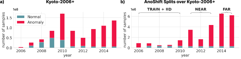
Figure 2: a) Yearly splits of the network traffic data from Kyoto-2006+ dataset, highlighting the proportion of normal and anomaly samples. b) Proposed train and test splits in our AnoShift benchmark. Considering that TRAIN and IID splits are sampled from the same time span, we have jointly represented them. Note that while for TRAIN , NEAR and FAR we extract the same number of normal samples per year, the IID split contains 10 times less normal samples. The anomaly samples are extracted such that we maintain the normal vs. anomaly proportion of the original data.

3.2.1 Experimental setup

Preprocess network traffic data

We use the 14 conventional features from the new version of the Kyoto dataset [2006-2015] and convert 3 of the 12 numerical features to categorical values by using an exponentially-scaled binning method between 0 and the maximum value of each feature, such that the bins have a higher density for smaller values and get increasingly wider towards larger values. We used a basis of 1.1, which results in 233 bins, where the width of the $i$th bin is given by: $bin_{i}=[1.1^{i}-1,1.1^{i+1}-1]$. We keep the original percentage features (9 out of 12 numerical features), which are discretized in 100 values. Therefore, our preprocessing results in a fixed vocabulary size and each possible token is known apriori. See in Fig. 3 a preprocessed sample. Our processing of the original dataset does not pose any privacy concerns since it does not contain any sensitive information, such as IP address. However, data binning constitutes another potential limitation in our work.

Figure 3: Examples of preprocessed Kyoto-2006+ instances. See Appendix A for details.

Metrics for anomaly detection

To analyze the performance of various models on our proposed benchmark, we use the labels (normal and anomaly) provided by the Kyoto-2006+ dataset. As we deal with imbalanced sets, we study the ROC-AUC metric and also evaluate the PR-AUC metric, for both inliers and outliers (note that for a random classifier, PR-AUC for a specific class is close to the ratio of data in that specific class). We report the IID, NEAR and FAR performances as the arithmetic mean of performances over their associated yearly splits.

4 Distribution shift analysis

We perform an in-depth analysis of the proposed benchmark from three points of view. First, we study the inherent non-stationarity of the considered data, highlighting the natural shift between the years, considering both simple, per feature metrics and more complex metrics between distributions (Sec. 4.1). Second, we analyze various anomaly detection models, highlighting the performance decrease when dealing with testing data that is temporarily distant from the training set (Sec. 4.2). Third, we discuss the importance of acknowledging the data shift and emphasize the positive impact of a basic distillation technique over the standard IID approach (Sec. 4.3). We add supplementary discussions on the method in Appendix A.1.

We run our experiments on an internal cluster with multiple GPU types: GTX 1080 Ti, GTX Titan X, RTX 2080 Ti, RTX Titan. We estimate that we need 5 days to reproduce the experiments on 1 GPU. The CPU training for OC-SVMs, IsolationForest, and LOF benchmarks takes  3 days.

4.1 Inherent non-stationarity

Visualization of the data shifts

For a visual interpretation of the yearly shift, we have considered the unsupervised t-SNE [46] to illustrate the high dimensional data structure (PCA visualization available in Appendix  A). In Fig. 4 we introduce the comparison between pairs of yearly splits and the whole figure can be interpreted as a similarity matrix, each cell $(i,j)$ illustrating the similarity between point clouds of year $i$ vs. year $j$. Each row illustrates the point clouds of the corresponding year over all the other point clouds. At the same time, each column presents the point clouds of the corresponding year below all the other point clouds for a better understanding of the distribution shifts. We observe that point clouds move away as we increase the temporal gap between their corresponding years. This confirms our intuition that the analyzed network traffic data is continuously shifting in time and emphasizes the need for a benchmark as AnoShift that can efficiently test the robustness of models under this inherent non-stationarity of natural data.

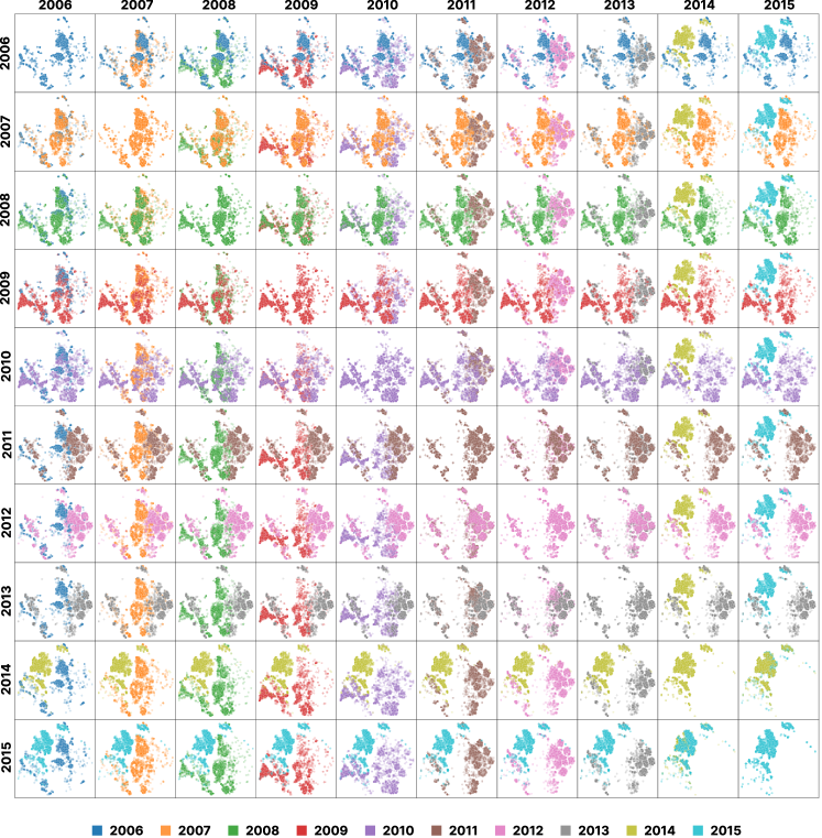
Figure 4: Comparison between yearly splits using t-SNE visualization. We observe that the discrepancy between point clouds increases with the temporal distance between splits, colors becoming more separated over time. The analysis is performed considering 2k randomly sampled points per split. Follow the 2007 row: see the orange cluster on top of clusters associated to the other years. It is very similar to its neighbours 2006-2008, and the similarity diminishes in time (see 2015).

Per-feature shift

We further analyze whether the dataset’s statistics at the feature level are changing from one year to another. Recall that we have 2 categorical features and 12 numerical ones. We extract the normalized histogram per year for each feature and compute the Jeffreys divergence [15] between those histograms. The Jeffreys divergence is a commonly used symmetrization for Kullback-Leibler divergence [21]: $KL(p,q)+KL(q,p)$, and it is proven to be both symmetric and non-negative. We highlight that such an analysis can only illustrate simple scenarios, studying the distribution change from the perspective of single feature changes. With all the considered baselines from Sec.4.2, we have observed a significant decrease in performance for the years 2014 and 2015, leading to the intuition that this subset may have substantial differences from the others. Consequently, in Fig. 5, we illustrate the Jeffreys divergence for two features that we find to have a large 2014-2015 distance, but also for a third one that has significant high values in the distance map on other years than the two.

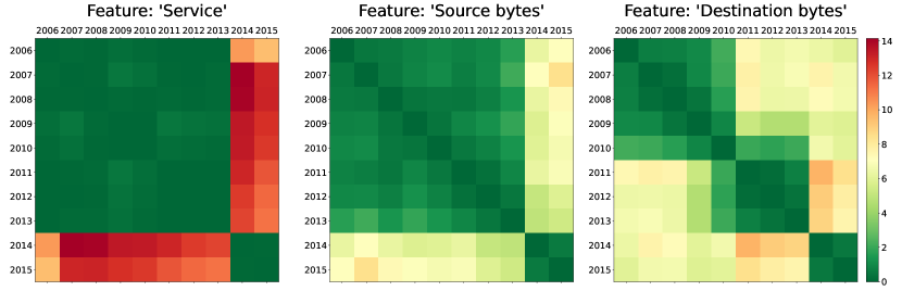
Figure 5: Jeffreys divergence between Kyoto years. First two images represent features with a large 2014-2015 distance. The $3^{rd}$ one is for a feature with significant difference between the histograms across years. Note that it is difficult to predict the performance of the method on a new split, only based on those per feature distances between distributions.

General shift

We next explore the distribution differences between dataset splits over time by using the Optimal Transport Dataset Distance method (OTDD) [3]. OTDD relies on optimal transport, a geometric method for computing distances between probability distributions for comparing datasets. This analysis shows how the splits move away from each other over time (see Fig. 6). Compared with the per feature approach, this method allows us to gain a better intuition for the performance on a new split, giving us a single distance based on all features. We observe how the inliers (first image) nicely distances in OTDD value, directly correlated with the distance in time. As for the outliers (third image), it is noticeable that they are quite different between the splits of the first years. We notice that the distances between inliers and outliers (in the middle) show that FAR years’ outliers are similar to TRAIN years’ inliers, an observation that we empirically confirm in Tab. 1, where all models suffer from a steep descent in performance (bellow random). We run the method with the default parameters for DatasetDistance, over the standardized input of Kyoto, with one-hot encoded categorical variables, $3$ times, with a randomly sampled 5k entries per year.

Figure 6: Optimal Transport Dataset Distance for Kyoto. See distances between inliers (first), inliers and outliers (second), and outliers (third). The distances from inliers generally increase as you move further from the diagonal, showing large distances between TRAIN and FAR data. Moreover, notice in second image how outliers in the FAR splits are quite similar with inliers from TRAIN, also explaining the abrupt performance drop on farther data (Tab. 1).

4.2 Impact on IID models

We introduce the AnoShift benchmark to understand better the impact of data shifts that naturally appear over time on the performance of anomaly detection models. We hope that the proposed splits will push forward the research in this direction and help build more robust models that can deal with mild to severe distribution changes between test and training sets. In this context, in the current section, we will study the performance degradation of various anomaly detection approaches, from IID to NEAR and FAR testing splits.

Anomaly detection models

We have considered several unsupervised baselines, ranging from more classical approaches, like Isolation Forest [27], OC-SVM [39], LocalOutlierFactor(LOF) [5] and recent ECOD [24] and COPOD [23], to deep learning ones, like SO-GAAL [28], deepSVDD [36], AE [1] for anomalies, LUNAR [14], InternalConstrastiveLearning [41] and our proposed transformer for anomalies model, based on the BERT [11] architecture. For part of the baselines, we have employed the PyOD library  [49].

BERT for anomalies

We use a simplified BERT architecture, without pretraining, with around 340k trainable parameters. We train the BERT model as a Masked Language Model (MLM), using a data collator that randomly masks a fraction $p$ of the input sequence and optimizing a cross-entropy loss function between the model predictions at mask positions and the original tokens. We derive a sequence anomaly score by randomly masking a fraction $p$ of tokens in the sequence and averaging the probabilities of the correct tokens at mask positions given by the classification layer over the vocabulary. At evaluation time, we average the score over $10$ mask samplings. A detailed description of the model is introduced in Appendix A. In our experiments, we used $p=15\%$.

In Table 1 we report the results of our experiments. Each baseline model was trained 3 times with a basic set of hyperparameters, and we reported the average results and the standard deviation. Both the OC-SVM and the LUNAR model were trained solely on $5\%$ of the TRAIN set to reduce the computational burden. For all of the considered models, except ECOD, we observe a performance degradation between NEAR and FAR splits, highlighting that these anomaly detection models cannot cope with the distribution shift. In the case of ECOD, the performances of both NEAR and FAR splits are below random, making their relative order irrelevant. The IID evaluation, which is the most popular methodology, proves to give an illusion of high performance, as the performance quickly degrades once we consider a testing set from a different period. The evolution is also presented in Appendix A-Fig. 10, illustrating ROC-AUC along with PR-AUC for inliers and outliers. We observe a rapid degradation for inliers PR-AUC, indicating that normal data distribution is continuously changing, and the outliers detection may not be reliable. These experiments highlight the issues of current anomaly detection models and prove the benefits of the AnoShift benchmark.

Table 1: Performance evolution over time, for classical and deep methods: IID vs NEAR vs FAR. Notice that the ROC-AUC is dropping over time in all cases, except for BERT and SO-GAAL methods, showing this is a property of the method, rather than a problem with the dataset. More precisely, those methods model the outliers very well in the NEAR split (see PR-AUC-out), while the PR-AUC-in is dropping, confirming the distribution shift over time (see Appendix A). On the FAR split, almost all methods perform under-random. Best scores per split are shown in bold: the highest scores on IID and NEAR are achieved by deepSVDD, but BERT is still competitive on these two splits. The best performance on FAR is surprisingly achieved by COPOD. PR-AUC for inliers and outliers are available in Appendix A-Fig. 10 and in Tab. 2.

		ROC-AUC $\uparrow$
Type	Baselines	IID	NEAR	FAR
Classical	OC-SVM [39] (train 5%)	76.86 $\pm$ 0.06	71.43 $\pm$ 0.29	49.57 $\pm$ 0.09
	IsoForest [27]	86.09 $\pm$ 0.54	75.26 $\pm$ 4.66	27.16 $\pm$ 1.69
	ECOD [24]	84.76	44.87	49.19
	COPOD [23]	85.62	54.24	50.42
	LOF [5]	91.50 $\pm$ 0.88	79.29 $\pm$ 3.33	34.96 $\pm$ 0.14
Deep	SO-GAAL [28]	50.48 $\pm$ 1.13	54.55 $\pm$ 3.92	49.35 $\pm$ 0.51
	deepSVDD [36]	92.67 $\pm$ 0.44	87.00 $\pm$ 1.80	34.53 $\pm$ 1.62
	AE [1] for anomalies	81.00 $\pm$ 0.22	44.06 $\pm$ 0.57	19.96 $\pm$ 0.21
	LUNAR [14] (train 5%)	85.75 $\pm$ 1.95	49.03 $\pm$ 2.57	28.19 $\pm$ 0.90
	InternalContrastiveLearning [41]	84.86 $\pm$ 2.14	52.26 $\pm$ 1.18	22.45 $\pm$ 0.52
	BERT [11] for anomalies	84.54 $\pm$ 0.07	86.05 $\pm$ 0.25	28.15 $\pm$ 0.06

Performance on FAR

With all tested baselines, we notice a significant decrease in performance for 2014-2015 years for inliers, which motivates us to further investigate the particularities of this subset. We observe a large distance in the Jeffreys divergence between 2014-2015 and the rest of the years for 2 features: service type and the number of bytes sent by the source IP (see Fig. 5). From the OTDD analysis in Fig. 6, we observe that: first, the inliers from FAR are very distanced to training years; and second, the outliers from FAR are quite close to the training inliers. One root cause of those events can be the steep increase of the "DNS" traffic percentage (from 4% to 37%, in 2013, and 2014 respectively). This contributes to the distribution shift on FAR, explaining the low performance.

Monthly evaluation

In Fig. 7, we take a closer look at the BERT’s performance at month granularity and break down performance on inliers and outliers. First, notice how the inliers’ performance gradually degrades over time, to an abrupt drop at farther months. This doubles the analysis from Sec. 4.1, where we notice the difference between the TRAIN years and FAR (through Jeffreys and OTDD experiments). Second, we observe that on IID years, the anomalies are modeled quite poorly by our language model, resulting in a slightly lower IID performance in comparison with NEAR.

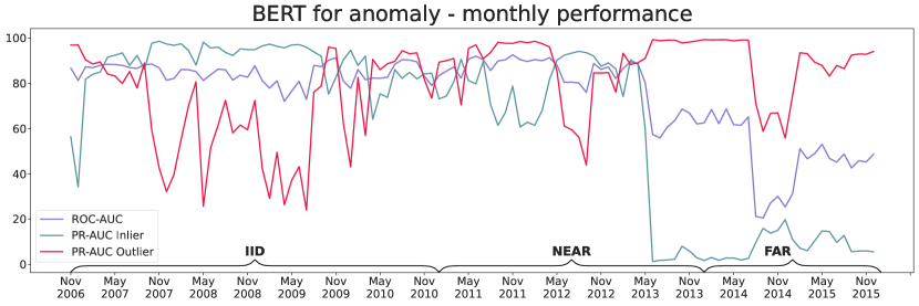
Figure 7: BERT for anomaly, evaluated on each month. We show the ROC-AUC, PR-AUC for inliers, and PR-AUC for outliers. The performance for the inliers is slowly decreasing during IID and NEAR splits, dropping suddenly just before the FAR split, showing how the language model fails to recognize inliers once it moves further apart from the training data. On the other hand, there are parts of the IID split where the outliers are quite poorly modeled, explaining the slightly poor performance of BERT on IID when compared with NEAR split.

4.3 Addressing the shifted data

We next compare the performance of a BERT model in 3 training regimes: iid, finetune, and knowledge distillation, for subsets of 300k entries from each year. We use 2006-2010 as training data and evaluate 2011-2015 as individual splits. First, in the a) iid mode, we use sets of data starting from 2006 and gradually add each successive split from the train period, initializing a new model for each subset. Next, in the b) finetune mode, we start from the iid model trained on 2006 and gradually finetune it on each successive year in the train period. Finally, in the c) distillation mode, we start from the iid model of 2006 and reinitialize a same-sized model for each new split, which becomes a student for the previous model by combining the MLM loss with a KL divergence loss with the teacher predictions on the current split. The best performance is achieved by the final distilled model for every test split (see Fig. 8), outperforming iid and finetune by over $3\%$ on average in ROC-AUC. It is worth noting that the effects of distillation are visible over time, with the iid method outperforming it in the first two iterations over the train splits. At all stages, the distillation method obtains the best performance on FAR data, providing a more robust training alternative to distribution shifts in data. The metrics are available in Appendix A-Tab. 3 and pseudocode for the training modes is available in Appendix A.2.

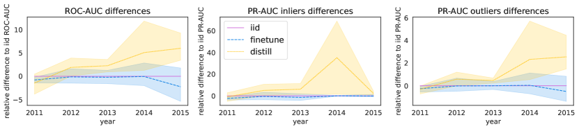
Figure 8: ROC-AUC, PR-AUC-in, PR-AUC-out for Finetune and Distill strategies, relative to the iid. The performance is averaged over all training subsets. Even though the strategies have a high variance in general, the distill is clearly more robust over time when compared to iid and finetune.

4.4 Discussions

MLM as anomaly detector

Even though the BERT model greatly exceeds the number of parameters and the complexity of other classical baselines, its generalization performance on farther data is extremely low. The anomaly performance in our case is based on the perplexity score when predicting several masked features in the sample. So if the features are not correlated, the MLM model might be unable to learn something useful, which might result in learning some specific training set biases, failing to generalize on temporarily distant data (eg. lower score on FAR wrt other baselines). We did not investigate this, but we consider it an interesting direction for future work.

MLM with the training vocabulary

In a real world setup, we expect that the fraction of tokens that are previously unseen during training increases with temporal distance. The evaluation score might get artificially inflated due to mapping of unseen features to the UNK token, as for farther points it is easier to predict UNK instead of the right word. Alongside the requirement of a discrete vocabulary, this is another limitation of vocabulary based methods as opposed to other classical approaches. We did not investigate these effects, but it might constitute an interesting direction for future work.

Other considered datasets

To emphasize the Kyoto-2006+ value, we briefly discuss here the other considered datasets and why we choose it in the end. We performed an in depth analysis over a large number of datasets, looking for two characteristics, essential for a distribution shift benchmark: it spreads over a large enough time-span, such that the distribution shift will naturally occur, rather than being synthetically injected, exhibiting sudden changes, and it is not solved already (existing methods do not report perfect scores on it). We first looked over a wide range of known 1. network traffic datasets for intrusion detection, and after analysing them we concluded that most are artificially created, with injected samples, in very restricted scenarios. Only Kyoto-2016 was a proper one, extended over a long enough period of time for showing a natural distribution shift. We next focused our attention on 2. system logs, since the time-span is usually more extensive in these dataset and the natural distribution shift is more probable to occur. But under our analysis (t-SNE, Jeffreys divergence, OTDD, multiple baselines), these datasets did not exhibit a clear distribution shift over time, so we decided to further analyse them until concludent results. Finally, we looked over 3. general multi-variate timeseries datasets, but the most popular ones are quite small and almost perfectly solved already. We leave this exact numbers for the considered datasets in the Appendix A.3.

5 Conclusion

Our approach highlights the true dimension of distribution shifts that appear in naturally and continuously evolving data streams. We analyze it in Kyoto-2006+ network traffic dataset that spans over 10 years from multiple angles: visually with t-SNE, statistically with histogram distances, and by measuring its magnitude with an Optimal Transport approach. Next, we propose AnoShift, a chronology-based benchmark for anomaly detection, to enable the development of models that generalize better and are more robust to shifts in data. Further, we show that by acknowledging the shift and addressing it, the performance can be improved, obtaining a +3% performance boost using a basic distillation technique.

Acknowledgments

We thank Razvan Pascanu for guiding us on how to approach the subject and Ioana Pintilie for helping us with baselines for the rebuttal.

Checklist

1. For all authors…

   1. Do the main claims made in the abstract and introduction accurately reflect the paper’s contributions and scope? [Yes]

   2. Did you describe the limitations of your work? [Yes] See Sec. 3.1 - paragraph 2.; Sec. 3.2.1 - paragraph 2.; Appendix A.1

   3. Did you discuss any potential negative societal impacts of your work?

      [No] Our work does not have a negative societal impact. Our benchmark proposal is tailored for finding intrusions in a computer network (not at the user level, but at the network level), by detecting anomalous traffic, in a more robust way than before, closer to the real scenario. One use-case is in the IT department of an company or university, where a person monitors the traffic alerts and prioritizes certain alerts based on the predictions of the robust models trained on our proposed benchmark.

   4. Have you read the ethics review guidelines and ensured that your paper conforms to them? [Yes]

2. If you are including theoretical results…

   1. Did you state the full set of assumptions of all theoretical results? [N/A]

   2. Did you include complete proofs of all theoretical results? [N/A]

3. If you ran experiments (e.g. for benchmarks)…

   1. Did you include the code, data, and instructions needed to reproduce the main experimental results (either in the supplemental material or as a URL)? [Yes] in the abstract and the appendix.

   2. Did you specify all the training details (e.g., data splits, hyperparameters, how they were chosen)? [Yes] see Sec. 4 and its subsections.

   3. Did you report error bars (e.g., with respect to the random seed after running experiments multiple times)? [Yes] For each of the tested methods in the main experiment, we run it 3 times, with different seeds.

   4. Did you include the total amount of compute and the type of resources used (e.g., type of GPUs, internal cluster, or cloud provider)? [Yes] see Sec. 4 - paragraph 2

4. If you are using existing assets (e.g., code, data, models) or curating/releasing new assets…

   1. If your work uses existing assets, did you cite the creators? [Yes] We used the existing Kyoto-2006+ dataset as raw data, as detailed in Sec. 3

   2. Did you mention the license of the assets? [N/A] The authors do not mention any kind of licence for the data, it is just publicly available.

   3. Did you include any new assets either in the supplemental material or as a URL? [Yes] We included a GitHub repository with code resources and a repository with the preprocessed data in the suplimentary material - see Appendix. B

   4. Did you discuss whether and how consent was obtained from people whose data you’re using/curating? [No] We had several emails with the authors, describing them our purpose and asking for additional information.

   5. Did you discuss whether the data you are using/curating contains personally identifiable information or offensive content? [Yes] see in Sec. 3.2.1

5. If you used crowdsourcing or conducted research with human subjects…

   1. Did you include the full text of instructions given to participants and screenshots, if applicable? [N/A]

   2. Did you describe any potential participant risks, with links to Institutional Review Board (IRB) approvals, if applicable? [N/A]

   3. Did you include the estimated hourly wage paid to participants and the total amount spent on participant compensation? [N/A]

Appendix A Appendix

Kyoto-2006+

When an attack occurs, the honeypot saves the network access pattern and other metadata and, at some point, might decide to reboot the system and rewrite back the original configuration. The authors deployed another machine in the network to generate normal traffic data, with a mailing server and a DNS service for a single domain. All traffic data from this server was labeled as clean (the logs also include other protocols for managing the machine over ssh or http and https). The 14 conventional features of the dataset includes 2 categorical features: connection service type and flag of the connection and 12 numerical features: connection duration, number of source and destination bytes, number of connections with corresponding IP addresses in a timeframe of two seconds and the percentage of connections accessing the same service and their rate of "SYN" errors, the prevalence of the connection’s source IP address and the requested service in the past 100 connections to the current destination IP (Kyoto features). The malicious traffic is further labeled using three software solutions: an Intrusion Detection Systems at the network level, an Antivirus product, and a shellcodes and exploits detector. In addition to those, the authors labeled other entries based on their prior history of connections from a specific IP and destination port. Additional features include source and destination IP addresses and ports, timestamp and protocol. We note that the generality of the original dataset imposes several limitations for our benchmark. More specific, the diversity of the normal traffic in a honeypot setup is quite restricted. Also, since the labeling is done using existing software and rules, the dataset’s anomalies might be underestimated.

Visualization of the data shifts with PCA

For completeness, in Fig. 9 we illustrate the distribution shift between years using a PCA visualization of the point clouds associated with each year. We observe similar results as the t-SNE visualization presented in Fig. 4.

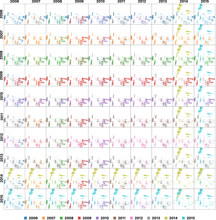
Figure 9: Comparison between yearly splits using PCA visualization. Similar to the t-SNE visualization, we observe that the discrepancy between point clouds increases with the temporal distance between splits, colors becoming more separated over time.

Performance evolution over time

In Tab. 2 and Fig. 10 we present the full evaluation of considered baseline models on IID, NEAR and FAR splits.

Training strategies for data shift

In Tab. 3 we present the full ROC-AUC, and PR-AUC for inliers and outliers, for all three training strategies: iid, finetune and distill.

BERT for Anomalies

We propose a simplified BERT architecture for detecting anomalies. The network input is tokenized by a WordLevel tokenizer which obtains tokens for the individual events in a system log sequence and, conversely, for the individual features of network traffic. Therefore, we have fixed-length sequences for Kyoto-2006. We train the BERT model as a Masked Language Model (MLM), using a data collator that randomly masks $p\%$ of the input sequence, by optimizing a cross-entropy loss function between the model predictions at mask positions and the original tokens. We derive a sequence anomaly score by randomly masking $p\%$ of tokens in the sequence and averaging the probabilities of the correct tokens at mask positions given by the classification layer over the vocabulary. The model is not pretrained and consists of two hidden layers of size $120$, an intermediate size of $192$ and $6$ attention heads. It has a hidden dropout and attention dropout probabilities of $0.1$, an epsilon of $1e-12$ for the normalization layer and a $0.02$ standard deviation range for the truncated normal weight initialization. Our architecture totals $342135$ trainable parameters. For training we mask $p=15\%$ of the input sequence and at evaluation time, we average over $n=10$ mask samplings.

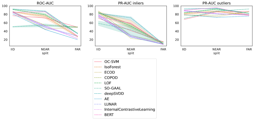
Figure 10: Performance evolution over time: IID vs NEAR vs FAR. We follow the evolution of ROC-AUC and PR-AUC for inliers and outliers. We observe a large performance gap between the considered splits, correlated with the temporal distance from the training set. (Best viewed in color)

Table 2: Performance evolution over time for unsupervised methods: IID vs NEAR vs FAR. We report beside the ROC-AUC metric, also the PR-AUC for inliers and PR-AUC for outliers. With bold are the best results per split.

Type	Unsupervised Baselines	IID	NEAR	FAR
		ROC-AUC (%) $\uparrow$
Classical	OC-SVM [39] (train 5%)	76.86 $\pm$ 0.06	71.43 $\pm$ 0.29	49.57 $\pm$ 0.09
	IsoForest [27]	86.09 $\pm$ 0.54	75.26 $\pm$ 4.66	27.16 $\pm$ 1.69
	ECOD [24]	84.76	44.87	49.19
	COPOD [23]	85.62	54.24	50.42
	LOF [5]	91.50 $\pm$ 0.88	79.29 $\pm$ 3.33	34.96 $\pm$ 0.14
Deep	SO-GAAL [28]	50.48 $\pm$ 1.13	54.55 $\pm$ 3.92	49.35 $\pm$ 0.51
	deepSVDD [36]	92.67 $\pm$ 0.44	87.00 $\pm$ 1.80	34.53 $\pm$ 1.62
	AE [1] for anomalies	81.00 $\pm$ 0.22	44.06 $\pm$ 0.57	19.96 $\pm$ 0.21
	LUNAR [14] (train 5%)	85.75 $\pm$ 1.95	49.03 $\pm$ 2.57	28.19 $\pm$ 0.90
	InternalContrastiveLearning [41]	84.86 $\pm$ 2.14	52.26 $\pm$ 1.18	22.45 $\pm$ 0.52
	BERT [11] for anomalies	84.54 $\pm$ 0.07	86.05 $\pm$ 0.25	28.15 $\pm$ 0.06
		PR-AUC inliers (%) $\uparrow$
Classical	OC-SVM [39] (train 5%)	70.84 $\pm$ 0.13	41.38 $\pm$ 0.29	15.12 $\pm$ 0.04
	IsoForest [27]	83.68 $\pm$ 3.47	57.06 $\pm$ 10.27	9.16 $\pm$ 0.18
	ECOD [24]	84.47	22.98	13.78
	COPOD [23]	87.86	29.25	14.55
	LOF [5]	84.11 $\pm$ 0.96	52.48 $\pm$ 4.56	10.15 $\pm$ 0.10
Deep	SO-GAAL [28]	58.65 $\pm$ 5.36	43.52 $\pm$ 11.62	10.68 $\pm$ 2.42
	deepSVDD [36]	82.62 $\pm$ 0.52	71.71 $\pm$ 4.85	10.02 $\pm$ 0.22
	AE [1] for anomalies	73.76 $\pm$ 0.09	26.16 $\pm$ 0.15	8.51 $\pm$ 0.01
	LUNAR [14] (train 5%)	78.91 $\pm$ 1.69	29.36 $\pm$ 2.58	9.33 $\pm$ 0.11
	InternalContrastiveLearning [41]	76.96 $\pm$ 2.12	27.28 $\pm$ 0.59	8.81 $\pm$ 0.05
	BERT [11] for anomalies	74.61 $\pm$ 0.13	58.94 $\pm$ 0.69	8.22 $\pm$ 0.02
		PR-AUC outliers (%) $\uparrow$
Classical	OC-SVM [39] (train 5%)	67.94 $\pm$ 0.21	85.70 $\pm$ 0.16	87.27 $\pm$ 0.02
	IsoForest [27]	81.46 $\pm$ 2.52	87.13 $\pm$ 2.08	78.33 $\pm$ 1.41
	ECOD [24]	78.37	74.48	85.9
	COPOD [23]	78.19	77.99	85.98
	LOF [5]	83.86 $\pm$ 0.98	92.34 $\pm$ 1.26	81.99 $\pm$ 0.05
Deep	SO-GAAL [28]	70.38 $\pm$ 0.28	87.71 $\pm$ 0.74	92.67 $\pm$ 0.13
	deepSVDD [36]	92.65 $\pm$ 0.64	94.15 $\pm$ 1.05	82.25 $\pm$ 0.48
	AE [1] for anomalies	78.99 $\pm$ 0.28	72.97 $\pm$ 0.38	75.71 $\pm$ 0.05
	LUNAR [14] (train 5%)	88.01 $\pm$ 1.03	80.91 $\pm$ 0.62	79.45 $\pm$ 0.30
	InternalContrastiveLearning [41]	89.08 $\pm$ 0.87	81.93 $\pm$ 0.39	77.55 $\pm$ 0.50
	BERT [11] for anomalies	89.83 $\pm$ 0.07	95.96 $\pm$ 0.06	78.38 $\pm$ 0.02

$$\hat{w_{j}}^{i}=\begin{cases}w_{j},&\text{if $mask_{i}$(j) = 0}\\ [MASK],&\text{if $mask_{i}$(j) = 1}\end{cases}$$ (1)

We repeat the masking process n times and average over all repeats to improve consistency. The anomaly score formula is depicted in equation 2, where we denote by $P_{M}$ the classification layer of the model of parameters $\theta_{M}$, by $Masks^{p}_{k}$ the set of random binary masks of length k and mask probability p, where $w_{t}$ are the initial tokens in the sequence and $\hat{w_{t}}^{i}$ is the j-th token in the sequence under mask i.

$$anomaly\_score([w_{1},w_{2},...,w_{t}])=\frac{\sum_{i=1..n}\sum_{j=1..t}^{mask_{i}\sim Masks^{p}_{t}}(1-P(\hat{w_{j}}^{i}))}{n}$$ (2)

$$P(\hat{w_{j}}^{i})=\begin{cases}1,&\text{if $mask_{i}$(j) = 0}\\ P_{M}(w_{j}|\theta_{M},[\hat{w_{1}}^{i},...,\hat{w_{t}}^{i}]),&\text{if $mask_{i}$(j) = 1}\end{cases}$$ (3)

We motivate this metric with the observation that inlier data should consist of common tokens with a high retrieval probability given by the distribution of the training set, while outliers should usually have either rare tokens or unusual combinations of features, within the context given by the unmasked tokens.

Table 3: Training strategies: ROC-AUC (%) for IID training vs Finetune vs Distil on Kyoto-2006+

	Train ON: 2006 ->	2007$\uparrow$	2008$\uparrow$	2009$\uparrow$	2010$\uparrow$
Strategy	Test split
IID	2011	88.95	88.93	88.27	89.92
	2012	95.85	90.96	86.28	86.63
	2013	94.05	87.00	80.79	81.87
	2014	28.56	24.35	22.64	21.16
	2015	49.01	42.20	37.05	34.07
Finetune	2011	88.56	87.18	87.3	89.92
	2012	95.78	89.31	85.18	89.14
	2013	94.19	85.29	79.36	84.06
	2014	32.98	22.50	20.50	20.57
	2015	53.39	38.99	30.98	30.04
Distil	2011	83.74	87.43	88.82	90.32
	2012	95.10	91.96	88.78	91.51
	2013	94.43	88.89	83.43	86.04
	2014	43.65	26.69	23.55	23.13
	2015	59.93	48.39	41.31	39.69

Impure training

Till now, we have considered anomaly detection models that were trained solely on the clean data of the TRAIN split. Further, we will study the performance evolution between IID, NEAR and FAR when the BERT model is trained on corrupt data containing mislabeled outliers in different percentages. In Fig. 11 we present the ROC-AUC for the 3 testing splits. We observe that the distribution shift is noticeable in the model performance even in this corrupt training setup. This validates the usefulness of the proposed chronological protocol when dealing with potentially mislabeled samples and highlights that the observed degradation over time is not a consequence of such dataset issues.

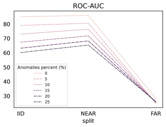
Figure 11: Performance evolution of our BERT model on IID, NEAR and FAR splits, when training on a corrupt set of samples, containing different percentages of mislabeled data points. (Best viewed in color)

Broader Impact

Our benchmark proposal is tailored for finding intrusions in a computer network (not at the user level, but at the network level), by detecting anomalous traffic, in a more robust way than before, closer to the real scenario. One use-case is in the IT department of an company or university, where a person monitors the traffic alerts and prioritizes certain alerts based on the predictions of the robust models trained on our proposed benchmark. Our work does not have a negative societal impact.

A.1 Discussions and future work

The inliers’ natural distribution

For being able to annotate large amount of data, the network datasets stay either in a clean space, where almost everything is normal, or in a "dark" one, where every connection is considered infected. Kyoto-2006+ lies in the second case, where the normal traffic is not very general, covering several behaviours. It might be interesting as future directions to find a way to combine the two cases towards a more general and unbiased dataset.

Pre-process through binning

We have performed the numerical to categorical conversion in order to make the dataset suitable for BERT based models, whose vocabularies would become too large otherwise. For a fair comparison, we consider it proper to use the same preprocessing for all the methods. We binarize 3 numerical features, transforming them into categorical ones (out of 12 total features). Namely, we convert only the float features: connection duration, number of source bytes and number of destination bytes into categorical ones (bins of values). We also perform experiments without preprocessing those numerical features (Tab. 4). Notice that the performance varies depending on the method and split, and it is not clear that one feature set is better than the other, over all the methods. Nevertheless, we see the same trend of performance drop across the three splits, supporting the claim of our work. Additionally, we observe that the evaluation on data without preprocessing numerical features instead of categorical ones achieves a better score on FAR. This might be explained by the fact that numerical binning induces a higher rarity of tokens in the FAR split compared to IID and NEAR, and therefore resulting in more uncertainty for the models.

Table 4: Compare different numeric feature preprocessing. Notice that it is not clear that one feature set is better than the other, over all the methods. Nevertheless, we see the same trend of performance drop across the splits, supporting the claim of our work.

Method	Feature binarization	IID	NEAR	FAR
		ROC-AUC (%) $\uparrow$
OC-SVM [39]	w	76.86	71.43	49.57
	w/o	81.87	71.24	50.95
IsoForest [27]	w	86.09	75.26	27.16
	w/o	94.41	95.13	32.81
ECOD [24]	w	84.76	44.87	49.19
	w/o	79.38	69.80	60.84
COPOD [23]	w	85.62	54.24	50.42
	w/o	79.03	65.67	60.12
AE [1]	w	81.00	44.06	19.96
	w/o	89.59	86.76	30.79

Gap between supervised and unsupervised learning

We evaluate several supervised learning methods for anomaly detection modeled as a binary classification task, on our AnoShift benchmark. We test several classical baselines: (SVM [9], RandomForest [25], XGBoost [8]), but also some attention-based deep learning methods (BERT with a classification head [10], TabNet [4], SAINT [42]). We report in Tab. 5 ROC-AUC, AUC-PR for Inliers and for Outliers for the supervised baselines, where we also included our unsupervised BERT baseline for comparison. We plotted the results in Fig. 12. We observe highly saturated scores on IID and NEAR and a major performance degradation on FAR. The highest performing methods on IID and NEAR, XGBoost, BERT and Saint, achieve the lowest scores on FAR across all baselines.

Full Kyoto-2006+ dataset

As previously described, AnoShift contains subsets of the full data, for allowing faster prototyping. We evaluate BERT for anomalies on the full Kyoto-2006+ yearly sets and observe that the ROC-AUC results are consistent with the subsets. The evaluation is performed on held-out test sets for each year and the results are available in Tab. 6. The subsets as well as the full sets used in our experiments are available at https://share.bitdefender.com/s/9D4bBE7H8XTdYDB.

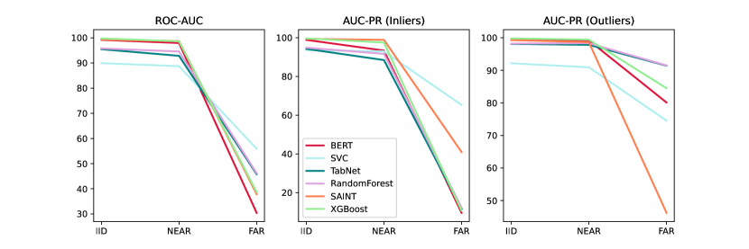
Figure 12: Performance evaluation for several supervised learning baselines in a binary classification task on the Kyoto-2006+ dataset.

Table 5: Performance evolution over time for supervised methods: IID vs NEAR vs FAR. We report the ROC-AUC, PR-AUC for inliers, and PR-AUC for outliers metrics. The performance degrades over time also in this supervised setting. Notice there is a large (and consistent) gap between the supervised methods and the unsupervised BERT baseline. Best score per split in bold.

Supervised Baselines	IID	NEAR	FAR
	ROC-AUC (%) $\uparrow$
XGB [8])	99.79 $\pm$ 0.01	98.63 $\pm$ 0.03	38.66 $\pm$ 0.32
SVM [9]	89.95 $\pm$ 0.81	88.74 $\pm$ 0.51	55.92 $\pm$ 0.21
RandomForest [25]	95.81 $\pm$ 0.13	94.58 $\pm$ 0.40	46.22 $\pm$ 0.73
SAINT [42])	99.33 $\pm$ 0.10	98.74 $\pm$ 0.09	37.85 $\pm$ 0.65
TabNet [4]	95.49 $\pm$ 0.28	92.86 $\pm$ 0.64	45.80 $\pm$ 0.57
BERT [10] - sup	99.20 $\pm$ 0.02	97.96 $\pm$ 0.08	30.42 $\pm$ 0.40
BERT [10] - unsup	84.54 $\pm$ 0.07	86.05 $\pm$ 0.25	28.15 $\pm$ 0.06
Difference (best sup, BERT-unsup)	+15.25	+12.69	+27.77
	PR-AUC Inliers (%) $\uparrow$
XGB [8])	99.64 $\pm$ 0.01	97.49 $\pm$ 0.02	10.72 $\pm$ 0.05
SVM [9]	93.57 $\pm$ 0.10	92.96 $\pm$ 0.20	65.27 $\pm$ 0.42
RandomForest [25]	94.85 $\pm$ 0.13	91.67 $\pm$ 0.91	12.27 $\pm$ 1.52
SAINT [42])	99.41 $\pm$ 0.08	98.89 $\pm$ 0.10	40.95 $\pm$ 0.42
TabNet [4]	94.24 $\pm$ 0.87	88.45 $\pm$ 1.89	11.63 $\pm$ 0.72
BERT [10] - sup	98.87 $\pm$ 0.04	93.37 $\pm$ 0.19	9.57 $\pm$ 0.06
BERT [10] - unsup	74.61 $\pm$ 0.13	58.94 $\pm$ 0.69	8.22 $\pm$ 0.02
Difference (best sup, BERT-unsup)	+25.03	+39.95	+57.05
	PR-AUC Outliers (%) $\uparrow$
XGB [8])	99.81 $\pm$ 0.01	99.44 $\pm$ 0.02	84.52 $\pm$ 0.21
SVM [9]	92.16 $\pm$ 0.22	90.93 $\pm$ 0.39	74.56 $\pm$ 0.14
RandomForest [25]	98.21 $\pm$ 0.06	98.34 $\pm$ 0.11	91.51 $\pm$ 0.12
SAINT [42])	99.28 $\pm$ 0.11	98.63 $\pm$ 0.07	46.21 $\pm$ 1.11
TabNet [4]	98.11 $\pm$ 0.04	97.83 $\pm$ 0.16	91.42 $\pm$ 0.27
BERT [10] - sup	99.51 $\pm$ 0.02	99.20 $\pm$ 0.04	80.12 $\pm$ 0.07
BERT [10] - unsup	89.83 $\pm$ 0.07	95.96 $\pm$ 0.06	78.38 $\pm$ 0.02
Difference (best sup, BERT-unsup)	+9.98	+3.48	+13.13

Table 6: BERT for anomalies ROC-AUC evaluation on the full sets in comparison with the subsets

		$\uparrow$ ROC-AUC
Split	2006	2007	2008	2009	2010	2011	2012	2013	2014	2015
Full	83.07	84.84	82.39	85.87	84.98	90.79	90.40	86.74	24.05	38.84
300k Subset	82.20	84.63	83.80	85.60	83.51	88.03	88.12	82.31	22.10	36.90

A.2 Pseudo-code for BERT training

We present the three algorithms for each training strategies: IID 1, Finetune 2, and Distilation 3.

Algorithm 1 IID training

$Model\leftarrow init\_model()$

$optimizer\leftarrow AdamW()$

$set\leftarrow shuffle(concat(set_{1},...,set_{n}))$

for $epoch\leftarrow[1,...,num\_epochs]$ do

     for $batch\sim set$ do

         $mask\sim random(batch.shape)<0.15$ $\triangleright$ Sample a binary mask of batch size with 0.15 probability

         $predictions=Model(batch*mask)$

         $loss\_batch=loss(predictions,batch)$ $\triangleright$ Reconstruction loss for masked tokens

         compute loss gradients

         perform optimizer step

     end for

end for

Algorithm 2 Finetune strategy

$Model\leftarrow init\_model()$

$loss\leftarrow CrossEntropy()$

$optimizer\leftarrow AdamW()$

for $set\leftarrow[set_{1},...,set_{n}]$ do

     for $epoch\leftarrow[1,...,num\_epochs]$ do

         for $batch\sim set$ do

              $mask\sim random(batch.shape)<0.15$ $\triangleright$ Sample a binary mask of batch size with 0.15 probability

              $predictions=Model(batch*mask)$

              $loss\_batch=loss(predictions,batch)$ $\triangleright$ Reconstruction loss for masked tokens

              compute loss gradients

              perform optimizer step

         end for

     end for

end for

Algorithm 3 Distillation strategy

$mlm\_loss\leftarrow CrossEntropy()$

$distil\_loss\leftarrow KL\_divergence()$

$optimizer\leftarrow AdamW()$

$Teacher\leftarrow$ train IID on $set_{1}$

for $set\leftarrow[set_{2},...,set_{n}]$ do

     $Student\leftarrow init\_model()$

     for $epoch\leftarrow[1,...,num\_epochs]$ do

         for $batch\sim set$ do

              $mask\sim random(batch.shape)<0.15$ $\triangleright$ Sample a binary mask of batch size with 0.15 probability

              $pred\_s=Student(batch*mask)$

              $pred\_t=Teacher(batch*mask)$

              $loss\_batch=mlm\_loss(pred\_s,batch)+distil\_loss(pred\_s,pred\_t)$

              compute loss gradients

              perform optimizer step

         end for

     end for

     $Student\leftarrow Teacher$

end for

A.3 Other considered datasets

We show here the detailed process of how we choose the Kyoto-2006+ dataset and why we consider it to be one of the few relevant in the distribution-shift context for stream-like data. We performed an in depth analysis over a large number of datasets. We wanted it to come from a stream-like data (as opposed to the less natural, existing benchmarks on images or text [26, 22, 44, 6, 20] and we for two characteristics that we consider essential for a distribution shift benchmark:

• It spreads over a large enough time-span, such that the distribution shift will naturally occur, (rather than being synthetically injected, exhibiting sudden changes)

• It is not solved already (existing methods do not report almost perfect scores on it)

Network traffic datasets

We first looked over a wide range of known network traffic datasets for intrusion detection (see Tab. 7), and after analysing them we concluded that most are artificially created, with injected samples, in very restricted scenarios. Only Kyoto-2016 was a proper dataset, extended over a long enough period of time for showing a natural distribution shift.

Table 7: Network traffic datasets.

Dataset	Number of samples	Time-span	Other details
CIC-IDS2017	3 mil	5 days	Different attack types per day
CSE-CIC-IDS2018	4.5 mil	17 days	Different attack types per day
UNSW-NB15	2.5 mil	2 days	too small
BoT-IoT	73 mil	4 days	too small
ToN-IoT	22 mil	6 days	too small
NSL-KDD	0.15 mil	45 days	max reported ROC-AUC 99%
LANL	1.6 mil	58 days	max reported ROC-AUC 99%
AAD	1.8 mil	90 days	internally build dataset, max ROC-AUC 98%
Kyoto-2006+	806M	10 years

System logs datasets

We next focused our attention on system logs, since the time-span is usually more extensive in these dataset and the natural distribution shift is more probable to occur. But under our analysis (t-SNE, Jeffreys divergence, OTDD, multiple baselines), these datasets did not exhibit a clear distribution shift over time, so we decided to further analyse them until concludent results. We used Drain and Spell as log parsers, and we report in Tab. 8 the results using the LogAnomaly [30] baseline.

Table 8: System logs datasets.

Dataset - Preprocessor	Number of samples	Time-span	IID (%)	NEAR (%)	FAR (%)	Split proportion
HDFS - Drain	11 mil	40h	54	66	57	6-6-6
BGL - Spell/Drain	4.7 mil	214 days	67/68	43/73	45/35	2-3-2
Thunderbird - Spell/Drain	211 mil	244 days	72/71	72/72	76/75	3-3-3
Liberty	266 mil	315 days				grouped anomalies
Spirit-CMU - Spell	272 mil	570 days	80	67	72	6-5-3

Multi-variate timeseries datasets

We next looked over general multi-variate timeseries datasets, but the most popular ones are quite small and almost perfectly solved already (see Tab. 9).

Table 9: Multi-variate timeseries datasets.

Dataset	Number of samples	Time-span	max reported unsup ROC-AUC (%)
SMAP - Soil Moisture Active Passive	0.5 mil	7-14 days	99
SWaT - Secure Water Treatment	0.9 mil	11 days	85
WADI - Water Distribution	0.96 mil	16 days	90
SMD - Server Machine Dataset	1.4 mil	35 days	99
MSDS - Multi-Source Distributed System	0.3 mil	days - months	91
PSM - Pooled Server Metrics		147 days	98
MSL - Mars Science Laboratory	0.13 mil	-	99
NAB - Numenta Anomaly Benchmark	0.37 mil	-	99
MBA - MIT-BIH Supraventricular Arrhythmia	0.2 mil	78 half-hour ECGs	99

Appendix B Appendix

Raw Kyoto dataset documentation

The dataset used in our proposed benchmark consists of a preprocessing of the Traffic Data from Kyoto University’s Honeypots and results from a discretization of the numerical features in the original dataset, such that a language-modelling approach can be easily applied. The original dataset consists of 14 conventional features and 10 additional features. The conventional features in the original dataset includes connection duration, type of service, number of source and destination bytes, server rate errors percentage and flag of connection. We keep all the conventional features and apply a exponentially-scaled binning over the continuous values (duration, number of source and destination bytes) which results in 233 bins and a discretization of the percentage features in 100 distinct values. As an observation, some of the 10 additional features (the source and destination IP addresses, source and destination port numbers) might be useful when designed models (eg. graphs) focusing on connections between the nodes in the system.

Our split proposal documentation

We propose a yearly split of the dataset and group adjacent years into Train, NEAR data and FAR data, which we use to highlight the performance degradation of several benchmarks in time, due to the distributional shift of the data which we demonstrate with a comprehensive analysis. In our proposed split, Train data consists of the first 4 years (2006-2010), Near data of the following 3 years (2011-2013) and Far data of the last two available years (2014-2015). We publish the data in splits of single years, in csv format. The columns 0 to 13 are the discretized conventional features in the Kyoto-2006+ dataset, preserving the original order, column 14 contains the complete timestamp. Columns 15, 16 and 17 correspond to the first 3 additional features in the original data, namely IDS_detection, Malware_detection and Ashula_detection, which indicates presence of alert triggers from the 3 IDS solutions: Symantec IDS, clamav and Ashula shellcode detector. Column 19 in the preprocessed dataset corresponds to the protocol used by the connection.

Intended uses

We hope that our proposed benchmark shifts the general direction of treating network intrusion detection towards a timely fashion that suffers from distributional shift, hereby providing a better suited evaluation protocol for upcoming research in this field.

URL to dataset download

We redirect our readers to the repository of the raw Kyoto dataset published by the Kyoto University at https://www.takakura.com/Kyoto_data/ and provide a repository of data under our proposed processing at https://share.bitdefender.com/s/9D4bBE7H8XTdYDB, with subsets of 300000 instances and heldout sets of 30000 instances for each split, maintaining the original inlier to outlier ratio from the original data in each split, as well as the full processed splits, with each full split except 2006 being provided in two parts. We make the remark that the 2006 split contains fewer instance, due to data collection debuting in November.

B.1 Code for dataset loading

We publish our code as a public GitHub repository https://github.com/bit-ml/AnoShift/, containing the data preprocessing script that transforms the original data in our format, sample data manipulation notebooks, license and additional information.

B.2 Author responsibility for violation of rights

There is no sensitive data leaked in the preprocessed dataset. The authors are not aware of any possible violation of rights and take responsibility for the published data.

B.3 Dataset hosting and long-term preservation

The authors take full responsibility for the availability of the processed data in the provided repository. However, no statement can be made about the availability of the raw Kyoto-2006+ data published by the Kyoto University, as it depends on Takakura.com. To avoid further problems, we have published our preprocessed version.

B.4 Licence

We release our code under a BSD 3-Clause License, therefore allowing the redistribution and use in source and binary forms, with or without modification, under the 3 clauses specified by the Berkeley Software Distribution License:

1. Redistributions of source code must retain the above copyright notice, this list of conditions and the following disclaimer.

2. Redistributions in binary form must reproduce the above copyright notice, this list of conditions and the following disclaimer in the documentation and/or other materials provided with the distribution.

3. Neither the name of the copyright holder nor the names of its contributors may be used to endorse or promote products derived from this software without specific prior written permission.

References

- Aggarwal [2017] Charu C Aggarwal. An introduction to outlier analysis. In Outlier analysis, pages 1–34. Springer, 2017.
- Ahmed et al. [2016] Mohiuddin Ahmed, Abdun Naser Mahmood, and Jiankun Hu. A survey of network anomaly detection techniques. J. Netw. Comput. Appl., 2016.
- Alvarez-Melis and Fusi [2020] David Alvarez-Melis and Nicolò Fusi. Geometric dataset distances via optimal transport. In NeurIPS, 2020.
- Arik and Pfister [2021] Sercan Ö Arik and Tomas Pfister. Tabnet: Attentive interpretable tabular learning. In Proceedings of the AAAI Conference on Artificial Intelligence, volume 35, pages 6679–6687, 2021.
- Breunig et al. [2000] Markus M. Breunig, Hans-Peter Kriegel, Raymond T. Ng, and Jörg Sander. LOF: identifying density-based local outliers. In SIGMOD International Conference on Management of Data, 2000.
- Cai et al. [2021] Zhipeng Cai, Ozan Sener, and Vladlen Koltun. Online continual learning with natural distribution shifts: An empirical study with visual data. In IEEE/CVF International Conference on Computer Vision, ICCV, 2021.
- Chen et al. [2021] Lei Chen, Shao-En Weng, Chu-Jun Peng, Hong-Han Shuai, and Wen-Huang Cheng. ZYELL-NCTU nettraffic-1.0: A large-scale dataset for real-world network anomaly detection. In IEEE International Conference on Consumer Electronics ICCE-TW, 2021.
- Chen et al. [2015] Tianqi Chen, Tong He, Michael Benesty, Vadim Khotilovich, Yuan Tang, Hyunsu Cho, Kailong Chen, et al. Xgboost: extreme gradient boosting. R package version 0.4-2, 1(4):1–4, 2015.
- Cortes and Vapnik [1995] Corinna Cortes and Vladimir Vapnik. Support-vector networks. Machine learning, 20(3):273–297, 1995.
- Devlin et al. [2018] Jacob Devlin, Ming-Wei Chang, Kenton Lee, and Kristina Toutanova. Bert: Pre-training of deep bidirectional transformers for language understanding. arXiv preprint arXiv:1810.04805, 2018.
- Devlin et al. [2019] Jacob Devlin, Ming-Wei Chang, Kenton Lee, and Kristina Toutanova. BERT: pre-training of deep bidirectional transformers for language understanding. NAACL, 2019.
- Dua and Graff [2007] Dheeru Dua and Casey Graff. Kdd-cup 1999, UCI machine learning repository, 2007. URL http://kdd.ics.uci.edu/databases/kddcup99/kddcup99.html.
- Gamal et al. [2020] Merna Gamal, Hala Abbas, and Rowayda A. Sadek. Hybrid approach for improving intrusion detection based on deep learning and machine learning techniques. In International Conference on Artificial Intelligence and Computer Vision, AICV, 2020.
- Goodge et al. [2022] Adam Goodge, Bryan Hooi, See-Kiong Ng, and Wee Siong Ng. Lunar: Unifying local outlier detection methods via graph neural networks. In Proceedings of the AAAI Conference on Artificial Intelligence, volume 36, pages 6737–6745, 2022.
- Jeffreys [1946] Harold Jeffreys. An invariant form for the prior probability in estimation problems. Proc. R. Soc. Lond., 1946.
- Jr. et al. [2019] Gilberto Fernandes Jr., Joel J. P. C. Rodrigues, Luiz Fernando Carvalho, Jalal Al-Muhtadi, and Mario Lemes Proença Jr. A comprehensive survey on network anomaly detection. Telecommun. Syst., 2019.
- K et al. [2018] Rahul-Vigneswaran K, R. Vinayakumar, K. P. Soman, and Prabaharan Poornachandran. Evaluating shallow and deep neural networks for network intrusion detection systems in cyber security. In International Conference on Computing, Communication and Networking Technologies, ICCCNT, 2018.
- Kent [2016] Alexander D. Kent. Cyber security data sources for dynamic network research. In Dynamic Networks and Cyber-Security, 2016.
- Khraisat et al. [2019] Ansam Khraisat, Iqbal Gondal, Peter Vamplew, and Joarder Kamruzzaman. Survey of intrusion detection systems: techniques, datasets and challenges. Cybersecur., 2019.
- Koh et al. [2021] Pang Wei Koh, Shiori Sagawa, Henrik Marklund, Sang Michael Xie, Marvin Zhang, Akshay Balsubramani, Weihua Hu, Michihiro Yasunaga, Richard Lanas Phillips, Irena Gao, Tony Lee, Etienne David, Ian Stavness, Wei Guo, Berton Earnshaw, Imran Haque, Sara M. Beery, Jure Leskovec, Anshul Kundaje, Emma Pierson, Sergey Levine, Chelsea Finn, and Percy Liang. WILDS: A benchmark of in-the-wild distribution shifts. In Proceedings of the International Conference on Machine Learning, ICML, 2021.
- Kullback and Leibler [1951] Solomon Kullback and Richard A Leibler. On information and sufficiency. The annals of mathematical statistics, 1951.
- Lazaridou et al. [2021] Angeliki Lazaridou, Adhiguna Kuncoro, Elena Gribovskaya, Devang Agrawal, Adam Liska, Tayfun Terzi, Mai Gimenez, Cyprien de Masson d’Autume, Tomás Kociský, Sebastian Ruder, Dani Yogatama, Kris Cao, Susannah Young, and Phil Blunsom. Mind the gap: Assessing temporal generalization in neural language models. In Advances in Neural Information Processing Systems, 2021.
- Li et al. [2020] Zheng Li, Yue Zhao, Nicola Botta, Cezar Ionescu, and Xiyang Hu. Copod: copula-based outlier detection. In 2020 IEEE International Conference on Data Mining (ICDM), pages 1118–1123. IEEE, 2020.
- Li et al. [2022] Zheng Li, Yue Zhao, Xiyang Hu, Nicola Botta, Cezar Ionescu, and George Chen. Ecod: Unsupervised outlier detection using empirical cumulative distribution functions. IEEE Transactions on Knowledge and Data Engineering, 2022.
- Liaw et al. [2002] Andy Liaw, Matthew Wiener, et al. Classification and regression by randomforest. R news, 2(3):18–22, 2002.
- Lin et al. [2021] Zhiqiu Lin, Jia Shi, Deepak Pathak, and Deva Ramanan. The CLEAR benchmark: Continual learning on real-world imagery. In NeurIPS Datasets and Benchmarks, 2021.
- Liu et al. [2012] Fei Tony Liu, Kai Ming Ting, and Zhi-Hua Zhou. Isolation-based anomaly detection. ACM Trans. Knowl. Discov. Data, 2012.
- Liu et al. [2019] Yezheng Liu, Zhe Li, Chong Zhou, Yuanchun Jiang, Jianshan Sun, Meng Wang, and Xiangnan He. Generative adversarial active learning for unsupervised outlier detection. IEEE Transactions on Knowledge and Data Engineering, 32(8):1517–1528, 2019.
- Lo et al. [2021] Wai Weng Lo, Siamak Layeghy, Mohanad Sarhan, Marcus R. Gallagher, and Marius Portmann. E-graphsage: A graph neural network based intrusion detection system. ArXiv, 2021.
- Meng et al. [2019] Weibin Meng, Ying Liu, Yichen Zhu, Shenglin Zhang, Dan Pei, Yuqing Liu, Yihao Chen, Ruizhi Zhang, Shimin Tao, Pei Sun, and Rong Zhou. Loganomaly: Unsupervised detection of sequential and quantitative anomalies in unstructured logs. In Artificial Intelligence, IJCAI, 2019.
- Mirsky et al. [2018] Yisroel Mirsky, Tomer Doitshman, Yuval Elovici, and Asaf Shabtai. Kitsune: An ensemble of autoencoders for online network intrusion detection. In Network and Distributed System Security Symposium, NDSS. The Internet Society, 2018.
- Moustafa and Slay [2015] Nour Moustafa and Jill Slay. UNSW-NB15: a comprehensive data set for network intrusion detection systems (UNSW-NB15 network data set). In Military Communications and Information Systems Conference, MilCIS, 2015.
- Pang et al. [2021] Guansong Pang, Chunhua Shen, Longbing Cao, and Anton van den Hengel. Deep learning for anomaly detection: A review. ACM Comput. Surv., 2021.
- Pérez et al. [2019] Daniel Pérez, Serafín Alonso, Antonio Morán Álvarez, Miguel A. Prada, Juan José Fuertes, and Manuel Domínguez. Comparison of network intrusion detection performance using feature representation. In Engineering Applications of Neural NetworksEANN, 2019.
- Ring et al. [2019] Markus Ring, Sarah Wunderlich, Deniz Scheuring, Dieter Landes, and Andreas Hotho. A survey of network-based intrusion detection data sets. Computers & Security, 86:147–167, 2019.
- Ruff et al. [2018] Lukas Ruff, Robert A. Vandermeulen, Nico Görnitz, Lucas Deecke, Shoaib A. Siddiqui, Alexander Binder, Emmanuel Müller, and Marius Kloft. Deep one-class classification. In International Conference on Machine Learning ICML, 2018.
- Sarhan et al. [2020] Mohanad Sarhan, Siamak Layeghy, Nour Moustafa, and Marius Portmann. Netflow datasets for machine learning-based network intrusion detection systems. In Big Data Technologies and Applications Conference, BDTA, and International Conference on Wireless Internet, WiCON, 2020.
- Sarhan et al. [2022] Mohanad Sarhan, Siamak Layeghy, and Marius Portmann. Towards a standard feature set for network intrusion detection system datasets. Mob. Networks Appl., 2022.
- Schölkopf et al. [1999] Bernhard Schölkopf, Robert C. Williamson, Alexander J. Smola, John Shawe-Taylor, and John C. Platt. Support vector method for novelty detection. In Advances in Neural Information Processing Systems, NIPS, 1999.
- Sharafaldin et al. [2018] Iman Sharafaldin, Arash Habibi Lashkari, and Ali A. Ghorbani. Toward generating a new intrusion detection dataset and intrusion traffic characterization. In International Conference on Information Systems Security and Privacy, ICISSP, 2018.
- Shenkar and Wolf [2021] Tom Shenkar and Lior Wolf. Anomaly detection for tabular data with internal contrastive learning. In International Conference on Learning Representations, 2021.
- Somepalli et al. [2021] Gowthami Somepalli, Micah Goldblum, Avi Schwarzschild, C Bayan Bruss, and Tom Goldstein. Saint: Improved neural networks for tabular data via row attention and contrastive pre-training. arXiv preprint arXiv:2106.01342, 2021.
- Song et al. [2011] Jungsuk Song, Hiroki Takakura, Yasuo Okabe, Masashi Eto, Daisuke Inoue, and Koji Nakao. Statistical analysis of honeypot data and building of kyoto 2006+ dataset for NIDS evaluation. In Proceedings of the First Workshop on Building Analysis Datasets and Gathering Experience Returns for Security, BADGERS EuroSys, 2011.
- Sun et al. [2022] Tao Sun, Mattia Segu, Janis Postels, Yuxuan Wang, Luc Van Gool, Bernt Schiele, Federico Tombari, and Fisher Yu. SHIFT: a synthetic driving dataset for continuous multi-task domain adaptation. In Computer Vision and Pattern Recognition, CVPR, 2022.
- Tavallaee et al. [2009] Mahbod Tavallaee, Ebrahim Bagheri, Wei Lu, and Ali A. Ghorbani. A detailed analysis of the KDD CUP 99 data set. In Symposium on Computational Intelligence for Security and Defense Applications, CISDA, 2009.
- van der Maaten and Hinton [2008] Laurens van der Maaten and Geoffrey Hinton. Visualizing data using t-SNE. Journal of Machine Learning Research, 2008.
- Verkerken et al. [2022] Miel Verkerken, Laurens D’hooge, Tim Wauters, Bruno Volckaert, and Filip De Turck. Towards model generalization for intrusion detection: Unsupervised machine learning techniques. J. Netw. Syst. Manag., 2022.
- Yang et al. [2019] Li Yang, Abdallah Moubayed, Ismail Hamieh, and Abdallah Shami. Tree-based intelligent intrusion detection system in internet of vehicles. In IEEE Global Communications Conference, GLOBECOM, 2019.
- Zhao et al. [2019] Yue Zhao, Zain Nasrullah, and Zheng Li. Pyod: A python toolbox for scalable outlier detection. Journal of Machine Learning Research, 20(96):1–7, 2019. URL http://jmlr.org/papers/v20/19-011.html.