Temperature dependence of the static quark diffusion coefficient

Abstract

The energy loss pattern of a low momentum heavy quark in a deconfined quark-gluon plasma can be understood in terms of a Langevin description. In thermal equilibrium, the motion can then be parametrized in terms of a single heavy quark momentum diffusion coefficient $\kappa$, which needs to be determined nonperturbatively. In this work, we study the temperature dependence of $\kappa$ for a static quark in a gluonic plasma, with a particular emphasis on the temperature range of interest for heavy ion collision experiments.

I Introduction

The charm and the bottom quarks provide very important probes of the medium created in the relativistic heavy ion collision experiments. Since the masses of both of these quarks are much larger than the temperatures attained in RHIC and in LHC, one expects these quarks to be produced largely in the early pre-equilibrated state of the collision. Heavy quark probes therefore provide a window to look into the early stages of the fireball.

In particular, the nature of the interaction of the heavy quarks with the thermalized medium is different from that of the light quarks. For energetic jets, radiative energy loss via bremsstrahlung is expected to be the dominant energy loss mechanism. For heavy quarks, the radiative energy loss is suppressed in a cone of angle $\sim m_{\scriptscriptstyle Q}/E$ dk . For heavy quarks of moderate energy, $E\lesssim 2m_{\scriptscriptstyle Q}$, collision with thermal quarks and gluons is expected to be the dominant mechanism of energy loss mt ; mustafa .

Even if the kinetic energy of the heavy quark is $\mathcal{O}(T)$, where $T$ is the temperature of the fireball, its momentum will be much larger than the temperature. Its momentum is, therefore, changed very little in a single collision, and successive collisions can be treated as uncorrelated. Based on this picture, a Langevin description of the motion of the heavy quark in the medium has been proposed svetitsky , mt ; mustafa . $v_{2}$, the elliptic flow parameter, can then be calculated in terms of the diffusion coefficient of the heavy quark in the medium. The diffusion coefficient has been calculated in perturbation theory svetitsky ; mt . While this formalism works quite well in explaining the experimental data for $R_{\scriptscriptstyle AA}$ and $v_{2}$ of the $D$ mesons (see annrev for a review), the diffusion coefficient required to explain the data is found to be at least an order of magnitude lower than the leading order (LO) perturbation theory (PT) result.

This is not a surprise per se, as the quark-gluon plasma is known to be very nonperturbative at not-too-high temperatures, and various transport coefficients have been estimated to have values very different from LOPT. However, this makes it important to have a nonperturbative estimate of the heavy quark diffusion coefficient. A field theoretic definition of the heavy quark diffusion coefficient to leading order of an $1/M$ expansion was given in ct ; clm . The next-to-leading order (NLO) calculation of the diffusion coefficient in perturbation theory cm was found to change the LO result by nearly an order of magnitude at temperatures $\lesssim 2T_{c}$. While the NLO correction is in the direction suitable for explaining the experimental data, the large change from LO to NLO indicates an inadequacy of perturbation theory in obtaining a reliable estimate for the diffusion coefficient in the temperature range of interest, and makes a nonperturbative estimate essential.

The first nonperturbative results for $\kappa$, using the formalism of clm and numerical lattice QCD in the quenched approximation (i.e., gluonic plasma), supported a value of $\kappa$ substantially different from LOPT and in the correct ballpark for HIC phenomenology prd11 . Of course, the plasma created in experiments is not a gluonic plasma, and one needs a full QCD calculation for phenomenology; but the fact that the quenched QCD result is of the right order of magnitude gives strong support for the Langevin description of the heavy quark energy loss. Later works bielefeld ; tum1 ; gflow improved on the calculations of prd11 . In particular, bielefeld ; gflow conducted a study at 1.5 $T_{c}$, and explored various systematics in the numerical calculation of $\kappa$. The focus of Ref. tum1 was a comparison with perturbation theory, and asymptotically high temperatures were explored. Meanwhile, a nonperturbative definition of the first correction to the static limit was discussed in blaine . Nonperturbative estimates of this correction have recently been carried out bb ; tum2 .

In this work we have carried out a study of the static quark momentum diffusion coefficient $\kappa$ in the temperature range $\lesssim 3.5T_{c}$, following the formalism of clm . The focus here is on studying the temperature dependence of $\kappa$ in the temperature range of interest for the relativistic heavy ion collision experiments. We extend the temperature range studied in prd11 to cover the entire temperature range of interest to the heavy ion community, and also improve the analysis technique, following Refs. bielefeld and bb . After explaining the formalism and our calculational techniques in Section II and Section III, respectively, we present the results of our study in Section IV. Combined with the $1/M$ correction terms calculated in bb , we can get the results for momentum diffusion coefficients for the charm and the bottom in the plasma. We discuss these results in Section V.

II Langevin formalism and nonperturbative definition of the momentum diffusion coefficient $\kappa$

In this section, we outline the formalism underlying our study. We first define the Langevin formalism for the heavy quark energy loss, as described in svetitsky , mt ; mustafa , and then give a nonperturbative definition of the diffusion coefficient, following ct ; clm .

The heavy quark momentum is much larger than the system temperature T: even for a near-thermalized heavy quark with kinetic energy $\sim T$, its momentum $p_{\scriptscriptstyle Q}\sim\sqrt{m_{\scriptscriptstyle Q}\,T}$, where $m_{\scriptscriptstyle Q}$ is the heavy quark mass. Individual collisions with the medium constituents with energy $\sim T$ do not change the momentum of the heavy quark substantially if $m_{\scriptscriptstyle Q}\gg T$. Therefore, the motion of the heavy quark is similar to a Brownian motion, and the force on it can be written as the sum of a drag term and a “white noise”, corresponding to uncorrelated random collisions:

$$\frac{dp_{i}}{dt}\ =\ -\eta_{\scriptscriptstyle D}\,p_{i}\ +\ \xi_{i}(t),\qquad\langle\xi_{i}(t)\xi_{j}(t^{\prime})\rangle\ =\ \kappa\ \delta_{ij}\ \delta(t-t^{\prime}).$$ (1)

The momentum diffusion coefficient, $\kappa$, can be obtained from the correlation of the force term:

$$\kappa\ =\ \frac{1}{3}\ \int_{-\infty}^{\infty}dt\ \sum_{i}\langle\xi_{i}(t)\,\xi_{i}(0)\rangle.$$ (2)

The drag coefficient, $\eta_{\scriptscriptstyle D}$, can be connected to the diffusion coefficient using standard fluctuation-dissipation relations kapusta :

$$\eta_{\scriptscriptstyle D}=\frac{\kappa}{2m_{\scriptscriptstyle Q}T}.$$ (3)

In the leading order in an expansion in $\frac{\textstyle 1}{\textstyle m_{\scriptscriptstyle Q}}$, the heavy quark interacts only with the color electric field of the plasma. Therefore the momentum diffusion coefficient $\kappa$ can be obtained from the electric field correlation function ct ; clm

$$G_{\scriptscriptstyle EE}(\tau)\ =\ -\frac{1}{3}\sum_{i=1}^{3}\frac{\left\langle\Re\,\mathrm{Tr}\;\,\left(U(L_{\tau},\tau)\;gE_{i}(\tau,\vec{x})\;U(\tau,0)\;gE_{j}(0,\vec{x})\right)\right\rangle}{\left\langle\Re\,\mathrm{Tr}\;\,U(L_{\tau},0)\right\rangle}\ \cdot$$ (4)

Here $U(\tau_{1},\tau_{2})$ is the gauge link in Euclidean time from $\tau_{1}$ to $\tau_{2}$ at spatial coordinate $\vec{x}$, $E(\tau,\vec{x})$ is the color electric field insertion at Euclidean time $\tau$, $L_{\tau}=1/T$ is the length of the Euclidean time direction, $\langle...\rangle$ indicates thermal averaging, and an average over the spatial coordinate $\vec{x}$ is implied (see clm for a formal derivation).

The spectral function, $\rho_{\scriptscriptstyle T}(\omega)$, for the force term is connected to $G_{\scriptscriptstyle EE}(\tau)$ by the integral equation kapusta

$$G_{\scriptscriptstyle EE}(\tau)\ =\ \int_{0}^{\infty}\frac{d\omega}{\pi}\ \rho_{\scriptscriptstyle T}(\omega)\ \frac{\cosh\omega(\tau-\frac{1}{2T})}{\sinh\frac{\omega}{2T}}\cdot$$ (5)

The momentum diffusion coefficient, $\kappa_{\scriptscriptstyle E}$, is then given by

$$\kappa_{\scriptscriptstyle E}\ =\ \lim_{\omega\to 0}\ \frac{2T}{\omega}\ \rho_{\scriptscriptstyle T}(\omega)\cdot$$ (6)

In this work we will use eq. (5), eq. (6) to calculate the momentum diffusion coefficient $\kappa_{\scriptscriptstyle E}$ for moderately high temperatures $T\lesssim 3.5T_{c}$. In particular, we will be exploring the temperature dependence of $\kappa_{\scriptscriptstyle E}/T^{3}$.

Note that $\kappa_{\scriptscriptstyle E}$ is the leading order estimate of $\kappa$ in an $\frac{\textstyle 1}{\textstyle m_{\scriptscriptstyle Q}}$ expansion. The $\mathcal{O}(m_{\scriptscriptstyle Q}^{-1})$ correction has been explored blaine : modulo some approximations, one can write

$$\kappa\approx\kappa_{\scriptscriptstyle E}\;+\;\frac{2}{3}\,\langle v^{2}\rangle\,\kappa_{\scriptscriptstyle B},$$ (7)

where $\langle v^{2}\rangle\;\approx\;\frac{\textstyle 3T}{\textstyle M_{\rm kin}}$ is the thermal velocity squared, and $M_{\rm kin}$ is the kinetic mass, of the heavy quark. $\kappa_{\scriptscriptstyle B}$ is the estimate of the diffusion coefficient one gets by replacing the electric fields with magnetic fields in eq. (5) and eq. (6). It has been calculated in Ref. bb for the gluonic plasma.

III Outline of the calculation

We calculated the electric field correlator $G_{\scriptscriptstyle EE}(\tau)$, eq. (4), for gluonic plasma using lattice discretization and numerical Monte Carlo techniques. On the lattice, the electric field was discretized, following clm , as

$$E_{i}(\vec{x},\tau)\ =\ U_{i}(\vec{x},\tau)\ U_{4}(\vec{x}+\hat{i},\tau)\ -\ U_{4}(\vec{x},\tau)\ U_{i}(\vec{x},\tau+1)\,\cdot$$

Then the lattice discretized $EE$ correlator takes the form

$$G_{\scriptscriptstyle EE}^{\scriptscriptstyle\rm bare}(\tau)\;=\;\frac{1}{V}\,\sum_{\vec{x}}\frac{C^{i}(\tau+1,\vec{x})+C^{i}(\tau-1,\vec{x})-2C^{i}(\tau,\vec{x})}{\prod_{x_{4}=0}^{L_{\tau}}U_{4}(\vec{x},x_{4})}$$ (8)

where $C^{i}(\tau,\vec{x})$ are Wilson lines at $\vec{x}$ with a hook of length $\tau$ in the $i$ direction, i.e.,

$$C^{i}(\tau,\vec{x})\;=\;U_{i}(\vec{x},0)\,\prod_{x_{4}=0}^{\tau-1}U_{4}(\vec{x}+\hat{i},x_{4})\,U_{i}^{\dagger}(\vec{x},\tau)\,\prod_{x_{4}=\tau}^{L_{\tau}}U_{4}(\vec{x},x_{4})\,\cdot$$

We have calculated the correlators $G_{\scriptscriptstyle EE}^{\scriptscriptstyle\rm bare}$ on the lattice at various temperatures $\lesssim 3.5T_{c}$. Equlibrium configurations for a gluonic plasma were generated at various temperatures by using lattices with temporal extent $N_{\tau}=\frac{\textstyle 1}{\textstyle T\,a(\beta)}$, where $a$ is the lattice spacing, and $\beta=\frac{\textstyle 6}{\textstyle g_{\scriptscriptstyle B}^{2}}$ is the coefficient of the plaquette term in the Wilson gauge action. The details of the lattices generated and the number of configurations at each parameter set is given in Table 1.

Table 1: Summary of runs and statistics.

$\beta$	$N_{\tau}$	$N_{\sigma}$	$T/T_{c}$	# sublattice	# update	# conf
7.05	20	64	1.50	5	500	1270
7.192	24	72	1.48	4	2000	2032
7.30	20	64	2.03	5	500	1200
7.457	24	80	2.04	4	500	1000
	20	80	2.45	6	500	730
7.634	30	96	2.01	5	2000	640
	24	96	2.51	4	2000	657
	20	96	3.01	5	2000	500
7.78	28	96	2.55	7	2000	678
	24	96	2.98	4	2000	536
	20	96	3.55	5	2000	522
7.909	28	96	2.96	7	2000	1100
	24	96	3.46	6	2000	967

The spatial extent of the lattices are chosen such that $LT>3$ and also the lattice is confined in the spatial direction. At various temperatures we have more than one lattice spacings; this allows us to estimate the discretization error, and to get the continuum result. Also for various values of the coupling, we have changed $N_{\tau}$ to change the temperature, keeping all the other parameters of the lattice unchanged. A comparison of the results from such lattices give us a direct handle on the temperature modification of $\kappa_{\scriptscriptstyle E}$.

Since we require very accurate correlation functions on lattices with large temporal extents, we have used the multilevel algorithm luscher in calculating eq. (8). We follow the implementation of the algorithm outlined in prd11 . The number of sublattices for the multilevel update, and the number of sublattice updates, are shown in Table 1, where each update consisted of (1 heatbath+3 overrelaxation) steps. Typically, a few parallel streams with independent random number seeds were used at each parameter sets. After a thermalization run which is many times the autocorrelation length, $\mathcal{O}(100)$ configurations were generated from each stream. The total number of configurations generated at each parameter set is shown in Table 1.

The temperature scale shown in Table 1 is obtained from the interpolation formula biescl

$$\log\frac{r_{0}}{a}\ =\ \left[\frac{\beta}{12\,b_{0}}\;+\;\frac{b_{1}}{2\,b_{0}^{2}}\,\log\frac{6b_{0}}{\beta}\right]\;\frac{1\,+\,c_{1}/\beta\,+\,c_{2}/\beta^{2}}{1\,+\,c_{3}/\beta\,+\,c_{4}/\beta^{2}}$$ (9)

where $b_{0}\,=\,11/(4\pi)^{2}$ and $b_{1}\,=\,102/(4\pi)^{4}$. The fit parameters $c_{i}$ are

$$c_{\{1,2,3,4\}}\ =\ \{-8.9664,\,19.21,\,-5.25217,\,0.606828\}$$ (10)

and $r_{0}T_{c}$ = 0.7457 biescl . Other ways of determining the temperature gives slightly different values: e.g., using the formula of Ref. ehk leads to a temperature which differs by $\sim$ 1-1.5 % at the higher $\beta$ values of Table 1. So we will effectively round off the temperature and, e.g., treat 3.46 $T_{c}$ and 3.55 $T_{c}$ in Table 1 as $\sim 3.5T_{c}$.

IV Analysis of the correlators and extraction of $\kappa/T^{3}$

IV.1 Discretization effect in $G_{\scriptscriptstyle EE}^{\scriptscriptstyle\rm bare}$

The $EE$ correlation functions $G_{\scriptscriptstyle EE}(\tau)$ are ultraviolet finite. The bare correlators $G_{\scriptscriptstyle EE}^{\scriptscriptstyle\rm bare}(\tau)$ require only finite renormalization:

$$G_{\scriptscriptstyle EE}^{\scriptscriptstyle\rm renorm}(\tau)\;=\;Z_{\scriptscriptstyle EE}(a(\beta))\,G_{\scriptscriptstyle EE}^{\scriptscriptstyle\rm bare}(\tau)\,\cdot$$ (11)

The renormalization coefficient $Z_{\scriptscriptstyle EE}(a)$ has been determined at one loop level in 1lp :

$$Z_{\scriptscriptstyle EE}\ =\ 1\,+\,\frac{2g_{\scriptscriptstyle B}^{2}C_{f}}{3}\;P_{1}\ \approx\ 1\,+\,0.1377g_{\scriptscriptstyle B}^{2}$$ (12)

where the lattice bare coupling $g_{\scriptscriptstyle B}^{2}=\frac{\textstyle 6}{\textstyle\beta}$, $C_{f}=\frac{\textstyle 4}{\textstyle 3}$, and $P_{1}=\int_{-\pi}^{\pi}\,\frac{\textstyle d^{4}k}{\textstyle(2\pi)^{4}}\,\frac{\textstyle 1}{\textstyle K^{2}}\,\approx 0.15493$.

After the renormalization, the correlator still shows cutoff effect, especially at short distances. A major part of this cutoff effect at short distances can be taken into account by a consideration of the discretization effect in the leading order. In leading order, the EE correlator takes the form francis

$$G_{\scriptscriptstyle EE}(\tau,LO) = g^{2}\,C_{f}\;G_{norm}(\tau),$$ (13)

$$G^{\scriptscriptstyle\rm Cont}_{\scriptscriptstyle\rm norm}(\tau) = \pi^{2}T^{4}\;{\rm cosec}^{2}(\pi\tau T)\ \left(\cot^{2}(\pi\tau T)\,+\,\frac{1}{3}\right)$$ (14)

$$G^{\scriptscriptstyle\rm Lat}_{\scriptscriptstyle\rm norm}(\tau) = \frac{1}{3a^{4}}\ \int\frac{d^{3}{k}}{8\pi^{3}}\frac{e^{\bar{k}(N_{\tau}-t)}\,+\,e^{\bar{k}t}}{e^{\bar{k}N_{\tau}}\,-\,1}\ \frac{\tilde{k}^{2}}{\sinh\bar{k}}$$ (15)

where the integration is over the Brillouin zone $(-\pi,\pi)$ and

$$\frac{\bar{q}}{2}\;=\;\operatorname{arcsinh}\frac{\tilde{q}}{2}\;,\qquad\tilde{q}^{2}\;=\;\sum_{i=1}^{3}\;4\,\sin^{2}\frac{q_{i}}{2}\ \cdot$$ (16)

A major part of the discretization effect can be accounted for by a comparison of eq. (14) with eq. (15): in particular, by defining an improved distance $\tau_{\rm imp}$ through sommer ; francis

$$G^{\scriptscriptstyle\rm Lat}_{\scriptscriptstyle\rm norm}(\tau_{\rm imp})\;=\;G^{\scriptscriptstyle\rm Cont}_{\scriptscriptstyle\rm norm}(\tau)\,\cdot$$ (17)

We have $G_{\scriptscriptstyle EE}^{\scriptscriptstyle\rm bare}(\tau)$ at multiple lattice spacings at each temperature. As noted in bielefeld ; tum1 before, we found that the use of $\tau_{\rm imp}$, eq. (17), reduces considerably the short distance discretization effect in $G_{\scriptscriptstyle EE}(\tau)$. In what follows, we have used $\tau_{\rm imp}$ to denote the distance scale for $G_{\scriptscriptstyle EE}^{\scriptscriptstyle\rm renorm}$.

At $T/T_{c}$ = 2, 2.5 and 3 we have three lattice spacings each. Using these correlators, we find the continuum extrapolated correlators at distances corresponding to $\tau_{\rm imp}$ for the finest lattice. We extrapolate $\frac{\textstyle G_{\scriptscriptstyle EE}}{\textstyle G^{\scriptscriptstyle\rm Lat}_{\scriptscriptstyle\rm norm}}(\tau)$ to $a\to 0$, where $\tau$ takes the values $\tau_{\rm imp}$ of the finest lattice at each temperature. The details of the method are presented in Appendix A. The correlators $\frac{\textstyle G_{\scriptscriptstyle EE}}{\textstyle G^{\scriptscriptstyle\rm Lat}_{\scriptscriptstyle\rm norm}}(\tau)$ for the different discretized lattices, and their continuum extrapolated value, are shown in Figure 1. The extrapolated ratio is now multiplied by $G^{\scriptscriptstyle\rm Cont}_{\scriptscriptstyle\rm norm}(\tau)$ to get the continuum extrapolated correlator. The calculation is done through a bootstrap analysis. For the bootstrap, the data is first blocked in blocks of size at least 2-3 times the autocorrelation time.

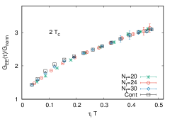
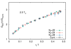
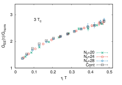
Figure 1: Continuum extrapolation of the correlator ratio $\frac{\textstyle G_{\scriptscriptstyle EE}}{\textstyle G^{\scriptscriptstyle\rm Lat}_{\scriptscriptstyle\rm norm}}(\tau)$, at (left) 2 $T_{c}$, (middle) 2.5 $T_{c}$, and (right) 3 $T_{c}$.

It is interesting to compare the continuum extrapolated correlator with perturbation theory. $G_{\scriptscriptstyle EE}$ has been calculated in perturbation theory to NLO in Ref. burnier ; in Figure 2 we compare the perturbative results of Ref. burnier with our nonperturbatively determined correlator lonlo . In Ref. burnier the scale for the running coupling has been set at

$$\mu_{\rm opt}\,\approx\,\max\,[7.57\,\omega,\;6.74\,T]$$ (18)

following the principle of minimal sensitivity. The LO and NLO bands in Figure 2 are obtained by varying $\mu\,\in\,[0.5,2]\,\mu_{\rm opt}$. This way of scale setting leads to a good agreement between the LO and the NLO calculation; but as Figure 2 shows, the perturbative estimates are very different from the nonperturbative results. We also show the LO results obtained by setting the scale in an intuitive way bielefeld :

$$\mu_{\rm fit}\,=\,\max\,[\omega,\pi T]\,\cdot$$ (19)

The band is obtained by varying this scale by a factor $[0.5,2.0]$ as before. As Figure 2 shows, the LO curve captures the main features of the nonperturbative result. However, the good agreement of perturbation theory with the lattice result in this case is misleading, as the NLO result changes strongly from the LO result and the lattice result. Guided by Figure 2, we will use the LO spectral function evaluated at the scale $\mu_{\rm fit}$ for modelling the ultraviolet part of the spectral function.

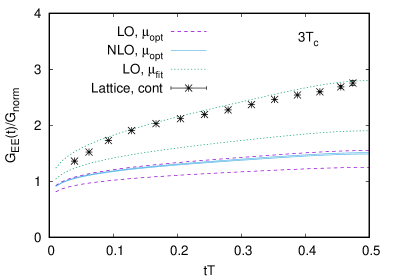
Figure 2: A comparison of the nonperturbatively obtained correlator $\frac{\textstyle G_{\scriptscriptstyle EE}}{\textstyle G^{\scriptscriptstyle\rm Lat}_{\scriptscriptstyle\rm norm}}(\tau)$ at $T=3T_{c}$ with the results of perturbation theory burnier . The LO and NLO results use an optimized scale (eq. (18)). Also shown is the LO result with the scale $\mu_{\rm fit}$ (eq. (19)). In each case, the bands for the perturbation theory are obtained by varying the scale by a factor of two in each direction from the scale mentioned above.

IV.2 Extraction of $\kappa$ from the correlators

A direct inversion of eq. (5) to get $\rho_{\scriptscriptstyle T}(\omega)$ is very difficult. Instead, to get an estimate of what kind of $\kappa_{\scriptscriptstyle E}$ is consistent with the $G_{\scriptscriptstyle EE}$ obtained, we have used some simple models for $\rho_{\scriptscriptstyle T}(\omega)$. Our models, and the analysis strategy, are similar to what was followed in Ref. bb for $G_{\scriptscriptstyle BB}(\tau)$, which, in turn, was influenced by earlier works prd11 ; bielefeld on $G_{\scriptscriptstyle EE}(\tau)$. The ultraviolet and the infrared parts of $\rho_{\scriptscriptstyle T}(\omega)$ are modelled with the simple forms

$$\rho_{\scriptscriptstyle UV}(\omega)\;=\;\frac{g^{2}(\mu_{\rm fit})\,C_{f}\,\omega^{3}}{6\pi},\qquad\rho_{\scriptscriptstyle IR}(\omega)\;=\;\kappa_{\scriptscriptstyle E}\,\omega\,,$$ (20)

where $\mu_{\rm fit}$ is defined in eq. (19). $\rho_{\scriptscriptstyle IR}(\omega)$ is the simplest form capturing the dissipative behavior of $\kappa_{\scriptscriptstyle E}$. The correlator eq. (4) does not have a transport peak, and is expected to have a smooth linear behavior in the infrared clm ; burnier , motivating $\rho_{\scriptscriptstyle IR}(\omega)$. $\rho_{\scriptscriptstyle UV}(\omega)$ is the known leading order form of the spectral function and the scale choice is motivated by Figure 2. The NLO spectral function is known burnier but, as Figure 2 shows, it is not clear that it will capture the ultraviolet behavior better except at very high $\omega$.

While both $\rho_{\scriptscriptstyle UV}(\omega)$ and $\rho_{\scriptscriptstyle IR}(\omega)$ are well-motivated, not much is known a-priori about the form of the spectral function in the intermediate $\omega$ regime. An ansatz, that allows $\rho_{\scriptscriptstyle T}(\omega)$ to continuously change from $\rho_{\scriptscriptstyle UV}(\omega)$ to $\rho_{\scriptscriptstyle IR}(\omega)$, is

$$\rho_{\scriptscriptstyle T}(\omega)\ =\ \max\left[c\,\rho_{\scriptscriptstyle UV}(\omega),\;\rho_{\scriptscriptstyle IR}(\omega)\right]$$ (21)

where we have introduced a parameter $c$ to take into account the uncertainty due to the scale choice and the use of the leading order form for $\rho_{\scriptscriptstyle UV}(\omega)$. $c$ is treated as a fit parameter. The best fit values we obtained for $c$ are close to 1, in the range 1-1.2.

A more smooth form of connecting $\rho_{\scriptscriptstyle UV}(\omega)$ with $\rho_{\scriptscriptstyle IR}(\omega)$ is

$$\rho_{\scriptscriptstyle T}(\omega)\ =\ \left[\sqrt{(c\,\rho_{\scriptscriptstyle UV}(\omega))^{2}\;+\;\rho_{\scriptscriptstyle IR}(\omega)^{2}}\right]\cdot$$ (22)

The form of eq. (22) has been argued to be theoretically better justified in bielefeld , gflow . Here again, the fit parameter $c\sim 1$ is introduced to account for the uncertainty in $\rho_{\scriptscriptstyle UV}(\omega)$. In our analysis we have treated eq. (21) and eq. (22) at par.

Instead of introducing a fit parameter $c$ as above, ref. bielefeld has suggested parametrizing the difference between the above forms (with $c$=1) and $\rho_{\scriptscriptstyle T}(\omega)$ in a sine expansion:

$$\left(1\,+\,\sum_{n}\,c_{n}\,\sin(\pi ny)\right),\qquad y\,=\,\frac{x}{1+x},\ \ x\,=\,\log\left(1\,+\,\frac{\omega}{\pi T}\right)\,\cdot$$

For the fit range we used, we found that one term in the expansion sufficed to fit our correlator. Therefore we have also tried the fit forms

$$\rho_{\scriptscriptstyle T}(\omega) = \left(1\,+\,c_{1}\,\sin\,\pi y\right)\ \left[\sqrt{\rho_{\scriptscriptstyle UV}(\omega)^{2}\;+\;\rho_{\scriptscriptstyle IR}(\omega)^{2}}\right]\,;$$ (23)

$$= \left(1\,+\,c_{1}\,\sin\,\pi y\right)\ \max\left[\rho_{\scriptscriptstyle UV}(\omega),\;\rho_{\scriptscriptstyle IR}(\omega)\right]\,.$$ (24)

In all our fits we have found $c_{1}$ to be small, $\in[0.02,0.12]$.

We perform the whole analysis for each of the model forms eq. (21), eq. (22), eq. (23) and eq. (24) in a bootstrap framework. Our final estimates of $\kappa_{\scriptscriptstyle E}$ are shown in Table 2 and in Figure 3. The details of the analysis can be found in Appendix A, where the estimates for each model are given in Table 3 and Figure 7. Our estimates in Table 2 and Figure 3 include the entire bands for eq. (22), eq. (21) and the central values for eq. (23), eq. (24).

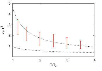
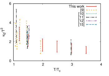
Figure 3: (Left) Our estimates for the range of $\kappa_{\scriptscriptstyle E}/T^{3}$ in the temperature range $\lesssim 3.5T_{c}$. Also shown (dotted lines) is the NLO perturbation theory estimate eq. (25) cm ; the band corresponds to varying the scale of the coupling $g^{2}(\mu)$ in the range $\mu\in[\pi T,4\pi T]$. (Right) A survey of other existing lattice results for $\kappa_{\scriptscriptstyle E}$ in gluonic plasma in the 1-4 $T_{c}$ temperature range. For visual clarity, points at 1.5 $T_{c}$ and 3 $T_{c}$ have been slightly shifted horizontally.

Table 2: Temperature dependence of $\kappa_{\scriptscriptstyle E}/T^{3}$

$T/T_{c}$	1.2	1.5	2.0	2.5	3.0	3.5
$\kappa_{\scriptscriptstyle E}/T^{3}$	2.1 - 3.5	1.5 - 2.8	1.0 - 2.3	0.9 - 2.1	0.8 - 1.8	0.75 - 1.5

There are other estimates of $\kappa_{\scriptscriptstyle E}/T^{3}$ for a gluonic plasma from the lattice. While Ref. prd11 studied the temperature range close to $T_{c}$, a detailed study at 1.5 $T_{c}$ was performed in Ref. bielefeld . A broad temperature range was studied in Ref. tum1 , with the main focus being very high temperatures. While the analysis techniques, in particular the spectral function models, vary, all these references used the multilevel algorithm and perturbative renormalization constants. Recently, Refs. gflow and tum2 have used gradient flow luscher-flow to get the renormalized $EE$ correlators at 1.5 $T_{c}$. We compare these studies with ours in the right panel of Figure 3. Within the uncertainties of our and other studies, our results agree very well with the other studies.

V Summary and Discussion

In this paper we have studied the electric field correlator, eq. (4), in a thermally equilibriated gluonic plasma at moderately high temperatures $T\lesssim 3.5T_{c}$. We investigated in detail the cutoff dependence of the correlators (Figure 1). With a simple set of models for the $EE$ spectral function $\rho_{\scriptscriptstyle T}(\omega)$, we then estimated the static quark momentum diffusion coefficient $\kappa_{\scriptscriptstyle E}$. The results are shown in Figure 3 and in Table 2.

$\kappa_{\scriptscriptstyle E}/T^{3}$ has been calculated to NLO in perturbation theory in cm . For SU(3) gluonic plasma, the NLO result is

$$\kappa_{\scriptscriptstyle E}/T^{3}\ =\ \frac{g^{4}C_{F}}{6\pi}\,T^{3}\,\left[\log\frac{2T}{m_{\scriptscriptstyle D}}\,+\,\xi\,+\,C\,g\right]$$ (25)

where $C_{F}=4/3,\,\xi\,\approx\,-0.64718,\ C\approx 2.3302$ and $m_{\scriptscriptstyle D}=gT$ in LO perturbation theory. This NLO result is shown in Figure 3 by the band bordered by the dotted lines; the band corresponds to evaluating $g^{2}$ at the scales $\mu\in[\pi T,4\pi T]$. The NLO results explain the data quite well. Note, however, that perturbation theory is inherently unstable here: the LO result is an order-of-magnitude smaller than NLO. In fact, if we omit the $\mathcal{O}(g)$ term in eq. (25), we will get a negative value for $\kappa_{\scriptscriptstyle E}/T^{3}$ in our temperature range burnier . The agreement of the NLO result with the nonperturbative results may indicate that the corrections beyond NLO are small.

It is of interest to compare our results on the temperature dependence of $\kappa_{\scriptscriptstyle E}$ with some other theoretical calculations. The estimate in Ref. ct is for $\mathcal{N}=4$ supersymmetric Yang-Mills theory, which is scale invariant. Clearly, $\kappa_{\scriptscriptstyle E}/T^{3}$ is temperature independent in such a theory. A different AdS-CFT based approach has been taken in Ref. andreev , where the drag term has been connected to the spatial string tension, $\sigma_{s}$. Eqn. (3) then connects $\kappa_{\scriptscriptstyle E}$ to $\sigma_{s}$. While the estimate of $\kappa_{\scriptscriptstyle E}/T^{3}$ obtained in Ref. andreev this way is close to our estimates, it provides a somewhat milder temperature dependence at higher temperatures.

While it is the momentum diffusion coefficient that enters the equations of Langevin dynamics and is of interest for the phenomenology of heavy quark thermalization, it has been the convention to quote the transport coefficient as the position space diffusion coefficient $D_{s}$. In particular, the combination

$$2\pi\,T\,D_{s}\;=\;\frac{4\pi}{\kappa/T^{3}}$$ (26)

is usually quoted. In the left panel of Figure 4 we plot $2\pi\,T\,D_{s}$ as obtained form our results of $\kappa_{\scriptscriptstyle E}$ using eq. (26).

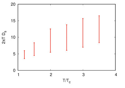
Figure 4: An estimation of the static quark diffusion coefficient, using eq. (26) and Table 2.

For phenomenological studies, one is interested in estimates of $\kappa$ for charm and bottom, rather than for the infinitely massive quarks. Using eq. (7) blaine one can provide such an estimate bb . In Figure 5 we show the separate estimates for $D_{s}^{c}$ and $D_{s}^{b}$, obtained using eq. (7) and eq. (26), and the $\kappa_{\scriptscriptstyle E}$ values of Table 2. The estimates of $\kappa_{\scriptscriptstyle B}$ are from ref. bb , supplemented by a calculation at 3 $T_{c}$, following exactly the same analysis techniques as in Ref. bb . The estimates we get for $D_{s}^{c}$ and $D_{s}^{b}$ are shown in Figure 5. The details can be found in Appendix A.

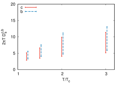
Figure 5: Estimate of $D_{s}^{c}$ and $D_{s}^{b}$, the spatial diffusion coefficients for the charm and bottom quarks, using eq. (7) and eq. (26). See text. For visual clarity, the points for $D_{s}^{b}$ have been slightly shifted horizontally.

$2\pi\,T\,D_{s}^{c,b}$ show a rising trend with temperature. The temperature dependence of $2\pi\,T\,D_{s}$ is of great interest to phenomenological studies cao ; duke ; das . In particular, in Ref. duke , using a parametric temperature dependence

$$2\pi\,T\,D_{s}\sim\alpha\;+\;\gamma\,\left(\frac{\textstyle T}{\textstyle T_{c}}-1\right),$$ (27)

$2\pi\,T\,D_{s}$ was estimated from the experimental data for $D$ meson using a Bayesian analysis. They quote the central values $\left(\alpha,\,\gamma\right)\,\sim\,\left(1.9,\,3.0\right)$, with $\alpha\sim 1-3$ being the $5-95$ percentile band duke . While our study is for quenched QCD, it is still interesting to check if the temperature dependences of $D_{s}^{c}$ and $D_{s}^{b}$ shown in Figure 5 are consistent with the simple parametrization of eq. (27). The answer is “yes” (admittedly, aided by the large uncertainties in our measurements), with $\left(\alpha,\,\gamma\right)$ = $\left(3.61(30),\,2.57(43)\right)$ for charm and $\left(3.99(35),\,3.08(54)\right)$ for bottom, respectively caution . For the static $D_{s}$, using the same parametrization we obtained $\alpha$ = 4.27(29) and $\gamma$ = 3.60(33). We also tried doing this linear fit for $2\pi\,T\,D_{s}$ from each of the models of Section IV.2. The results can be seen in Figure 8 and Table 4 in Appendix A. All of the model spectral functions indicate a positive slope of $2\pi\,T\,D_{s}$ with temperature. We emphasize that eq. (27) is a purely phenomenological fit: the temperature dependence of $D_{s}$ is of course more complicated, e.g., eq. (25).

VI Acknowledgements

We thank Mikko Laine for providing the perturbative curves in Figure 2, and for discussions. The computations presented in this paper were performed on the clusters of the Department of Theoretical Physics, TIFR, and on the ILGTI computing facilities of IACS and TIFR. We would like to thank Ajay Salve and Kapil Ghadiali for technical assistance. S.D. acknowledges support of the Department of Atomic Energy, Government of India, under Project Identification No. RTI 4002.

Appendix A Some details of the numerical analysis

Here we provide additional details of our numerical analysis in Section IV.

We do a detailed calculation at temperatures $T/T_{c}$ = 2, 2.5 and 3. At these temperatures we have correlators from three lattice spacings. We have estimated the continuum correlator from them, and calculated $\kappa_{\scriptscriptstyle E}$ from it. Our whole analysis is done in a bootstrap formalism. To get the continuum correlator, the average correlator for each bootstrap sample is B-spline interpolated, and the value of the correlation function at distances corresponding to the $\tau_{\rm imp}$ values of the finest lattice are obtained. Note that this typically involves an extrapolation at the smallest distance, but this is not a concern as this distance is not used in the fits. A very slight extrapolation is also required at the largest ($\tau\sim 1/2T$) distance point, but it is a very small extrapolation and we do not expect this to be a problem.

At short distances $\tau_{\rm imp}T\lesssim 0.15$ we see a clear discretization effect, which is approximately linear in $a^{2}$; we fit to a linear form to get the continuum correlator. For larger distances $\tau_{\rm imp}T>0.25$ the correlators do not show a clear discretization effect. In particular, for correlators at large distances $\tau_{\rm imp}T\gtrsim 0.3$ we found a constant fit to be more reasonable. We show examples of our continuum extrapolation at some representative distances in Figure 6. Note that we have also carried out the analysis with linear extrapolation at all distances; the $\kappa$ values obtained agree within errorbar.

To extract $\kappa_{\scriptscriptstyle E}$ from the continuum correlators using eq. (5), we have used the fit forms discussed in Section IV.2, and done a standard $\chi^{2}$ fit. The [16,84] percentile band of the bootstrap estimators of $\kappa_{\scriptscriptstyle E}$ is treated as the 1-$\sigma$ errorband. The results for the various fit forms are shown in Figure 7. Typically we get a good $\chi^{2}$ by taking the whole range except the two shortest distance points. We have, however, also varied $\tau_{\rm imp}^{\rm min}$. The results shown in Figure 7 include the variation with fit range, and any difference due to using linear vs constant extrapolation at large separations in Figure 6.

As mentioned in Section IV.2, we have also fitted the correlators from the individual lattices to the forms of Section IV.2. For this we have used $\tau_{\rm imp}^{\rm min}\sim 0.25/T$, where the discretization effect on the correlators is small. $\tau_{\rm imp}^{\rm min}$ is further varied within a small range. The bands shown in Figure 7 include the spread due to such a variation.

In Table 3 we show the final results for $\kappa_{\scriptscriptstyle E}/T^{3}$ using the different fit forms. The error estimate is conservative, covering the 1$\sigma$ interval obtaned from the continuum correlator and the correlators from lattices with $N_{t}\geq 24$.

Table 3: Results for $\kappa_{\scriptscriptstyle E}/T^{3}$ from the different fit forms of Section IV.2.

$T/T_{c}$	eq. (21)	eq. (22)	eq. (24)	eq. (23)
1.2	2.16-2.80	2.44-3.54	1.80-2.50	2.34-3.14
1.5	1.74-2.16	1.62-2.80	1.25-1.73	1.55-2.27
2	1.05-1.60	1.48-2.30	0.77-1.42	1.04-1.82
2.5	0.91-1.77	1.17-2.08	0.70-1.59	0.97-1.86
3	0.87-1.48	1.04-1.80	0.60-1.30	0.83-1.56
3.5	0.76-1.14	1.01-1.50	0.62-1.02	0.96-1.33

Table 3 also includes two temperatures where we have only two lattice spacings each, and 1.2 $T_{c}$ where we have reanalyzed the correlators on $N_{t}$=24 lattices calculated in Ref. bb . In these cases we have only fitted the individual lattices. The rest of the discussion is the same as above. The final result in these cases is taken from the $N_{t}$=24 lattices.

For the final result for $\kappa_{\scriptscriptstyle E}$ shown in Figure 3, we have treated the fit forms eq. (21) and eq. (22) at par, and conservatively quoted an error band that includes the bands for eq. (21) and eq. (22) in Table 3 and the central values of the bands for eq. (21) and eq. (22). These results are also shown in Table 2.

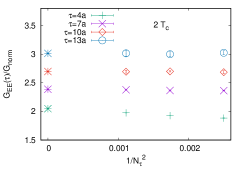
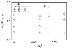
Figure 6: Illustration of the continuum extrapolation of the correlator normalized by $G_{norm}$. (Left) 2 $T_{c}$, (middle) 2.5 $T_{c}$ and(right) 3 $T_{c}$.

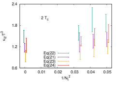
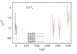
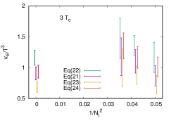
Figure 7: Results for $\kappa_{\scriptscriptstyle E}/T^{3}$ obtained at $T/T_{c}$ = 2 (left), 2.5 (middle) and 3 (right). Besides the continuum results, the results obtained from fitting individual lattices is also shown. See the text for details of the error band.

Using Table 3 and eq. (26) we can also make separate estimates for $2\pi\,T\,D_{s}$ for each form of the model $\rho_{\scriptscriptstyle T}(\omega)$ in Section IV.2. This is shown in Figure 8. The linearly rising behavior of each of these forms can then be separately fitted to the linear fit form eq. (27). The results of such a fit are shown in Table 4.

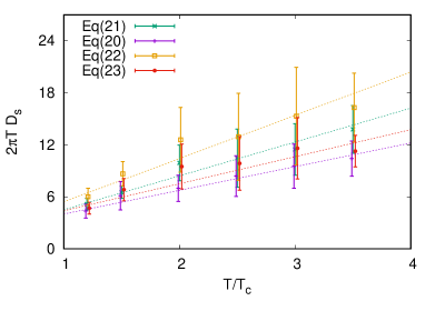
Figure 8: An estimation of the static quark diffusion coefficient, using eq. (26) and Table 2. Also shown are the best fits to a liear temperature dependence (eq. (27)).

Table 4: The fit parameters for eq. (27)

.

	eq. (22)	eq. (21)	eq. (23)	eq. (24)
$\alpha$	4.01(24)	4.51(27)	5.42(50)	4.39(45)
$\gamma$	3.91(39)	2.73(24)	4.99(71)	3.12(50)

In Figure 5 we show the estimates for $D_{s}^{c}$ and $D_{s}^{b}$ in the temperature range 1.2-3 $T_{c}$, using eq. (26), where $\kappa^{c}$ and $\kappa^{b}$ are obtained using eq. (7). The estimates for $\kappa_{\scriptscriptstyle B}$ are taken from Ref. bb , supplemented with a calculation at 3 $T_{c}$. The $BB$ correlator $G_{\scriptscriptstyle BB}(\tau)$ at 3 $T_{c}$ at different lattice spacings, normalized by the corresponding leading order correlator $\frac{\textstyle G_{\scriptscriptstyle BB}(\tau,LO)}{\textstyle g^{2}C_{f}}$ for lattice with the same $N_{\tau}$, are shown in Figure 9. We also show the corresponding continumm extrapolated correlator in the figure. The analysis for $\kappa_{\scriptscriptstyle B}$ at 3 $T_{c}$ follows that used in bb ; it is similar to the analysis for $\kappa_{\scriptscriptstyle E}$ outlined in Section III, except, following Ref. bb , the scale for the perturbative part of the $BB$ spectral function is taken to be $\mu_{\rm fit}^{\scriptscriptstyle B}\,=\,\rm{max}\,\left[\omega^{\frac{5}{11}}\left(\pi T\right)^{\frac{6}{11}},\pi T\right]$ instead of eq. (19). The results obtained for $\kappa_{\scriptscriptstyle B}$ for the different fit forms are also shown in Figure 9. Taking a band that includes the different fit forms, we obtain an estimate $\kappa_{\scriptscriptstyle B}/T^{3}\,\sim$ 0.6 - 1.3 at 3 $T_{c}$.

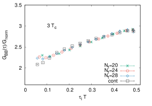
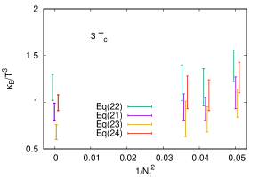
Figure 9: (Left) The correlator $G_{\scriptscriptstyle BB}(\tau)$ at 3 $T_{c}$ calculated at different lattice spacings, normalized by $G_{norm}=\frac{\textstyle G_{\scriptscriptstyle BB}(\tau,LO)}{\textstyle g^{2}C_{f}}$. Also shown is the continuum extrapolated correlator. (Right) Estimates of $\kappa_{\scriptscriptstyle B}/T^{3}$ at 3 $T_{c}$ obtained using the different fit forms. See text for explanation.

Following Ref. bb , $\langle v^{2}\rangle$ was estimated from a ratio of the susceptibilities calculated in vsq . This gives $\langle v^{2}\rangle\approx(0.76,0.40)$ for charm and bottom at 3 $T_{c}$, respectively (the values at the lower temperatures are given in Ref. bb ). At such temperatures, a nonrelativistic treatment of charm may be questionable. We find that the $\mathcal{O}(m_{\scriptscriptstyle Q}^{-1})$ corrections to $\kappa$, eq. (7), are $\sim$ 38 % for charm and $\sim$ 20 % for bottom.

From the results for $\kappa^{c}$ and $\kappa^{b}$, $D_{s}^{c}$ and $D_{s}^{b}$ can be obtained using eq. (26). Since the range for $\kappa$ is dominated by systematics, we simply find the range of $D_{s}$ by using eq. (26) for the lower and upper bound of the range for $\kappa$. The results for $2\pi\,T\,D_{s}^{c,b}$ obtained this way are given in Table 5 and shown in Figure 5.

Table 5: The estimates for $2\pi\,T\,D_{s}^{c,b}$, from eq. (26) and eq. (7).

	1.2 $T_{c}$	1.5 $T_{c}$	2 $T_{c}$	3 $T_{c}$
$2\pi\,T\,D_{s}^{c}$	2.9 - 5.1	3.5 - 6.6	4.0 - 9.9	5.1 - 11.4
$2\pi\,T\,D_{s}^{b}$	3.3 - 5.6	4.0 - 7.6	4.7 - 11.2	5.9 - 13.1

References

- (1) Y. Dokshitzer & D. Kharzeev, Phys. Lett. B 519 (2001) 199.
- (2) G. D. Moore and D. Teaney, Phys. Rev. C 71 (2005) 064904.
- (3) M. G. Mustafa, Phys. Rev. C 72 (2005) 014905.
- (4) B. Svetitsky, Phys. Rev. D 37 (1988) 2484.
- (5) X. Dong, Y-J. Lee & R. Rapp, Ann. Rev. Nucl. Part. Sci. 69 (2019) 417.
- (6) J. Casalderrey-Solana and D. Teaney, Phys. Rev. D 74 (2006) 085012.
- (7) S. Caron-Huot, M. Laine & G. Moore, J. H. E. P. 04 (2009) 053 (0901.1195).
- (8) S. Caron-Huot & G. Moore, J. H. E. P. 0802 (2008) 081.
- (9) D. Banerjee, S. Datta, R. Gavai & P. Majumdar, Phys. Rev. D 85 (2012) 014510 (1109.5738).
- (10) A. Francis, O. Kaczmarek, M. Laine, T. Neuhaus & H. Ohno, Phys. Rev. D 92 (2015) 116003.
- (11) N. Brambilla, V. Leino, P. Petreczky & A. Vairo, Phys. Rev. D 102 (2020) 074503.
- (12) L. Altenkort, A. Eller, O. Kaczmarek, L. Mazur, G. Moore & H.-T. Shu, Phys. Rev. D 103 (2021) 014511.
- (13) A. Bouttefeux and M. Laine, J. H. E. P. 12 (2020) 150.
- (14) D. Banerjee, S. Datta & M. Laine, J. H. E. P. 08 (2022) 128 (arXiv:2204.14075).
- (15) N. Brambilla, V. Leino, J. Mayer-Steudte & P. Petreczky, arXiv:2206.02861.
- (16) J. Kapusta & C. Gale, Finite Temperature Field Theory: Principles and Applications, 2nd Edition. Cambridge University Press, 2006.
- (17) M. Lüscher and P. Weisz, J. H. E. P. 0109 (2001) 010, J. H. E. P. 0207 (2002) 049.
- (18) Y. Burnier, H-T. Ding, O. Kaczmarek, A-L. Kruse & M. Laine, J. H. E. P. 11 (2017) 206.
- (19) R.G. Edwards, U.M. Heller & T.R. Klassen, Nucl. Phys. B 517 (1998) 377
- (20) C. Christensen & M. Laine, Phys. Lett. B 755 (2016) 316 (1601.01573).
- (21) A. Francis, O. Kaczmarek, M. Laine & J. langelage, PoS LATTICE2011 (arXiv:1109.3941).
- (22) R. Sommer, Nucl. Phys. B411 (1994) 839.
- (23) Y. Burnier, M. Laine, J. Langelage, L. Mether, J. H. E. P. 08 (2010) 094
- (24) Note that the EE correlator at LO does not have a diffusion term; the leading order estimate for comes from the EE correlator calculated at NLO.
- (25) M. Lüscher, J. H. E. P. 08 (2010) 071.
- (26) O. Andreev, Mod. Phys. Lett. A 33 (2018) 1850041.
- (27) Y. Burnier & M. Laine, J. H. E. P. 11 (2012) 086.
- (28) S. Cao, et al., Phys. Rev. C 99 (2019) 054907.
- (29) Y. Xu, J. Bernhard, S. Bass, M. Nahrgang & S. Cao, Phys. Rev. C 97 (2018) 014907.
- (30) S. K. Das, F. Scardina, S. Plumari & V. Greco, Phys. Lett. B 747 (2015) 260.
- (31) Here we have done a simple analysis, treating the error band in Table 2 as a statistical 1 band. The error band in the table is dominated by systematic errors. So while the fit does indicate that the data is inconsistent with a flat behavior with temperature, one should not attribute the standard 1 interpretation to the error bars quoted for the fit parameters.