Understanding Instance-Level Impact of Fairness Constraints

Abstract

A variety of fairness constraints have been proposed in the literature to mitigate group-level statistical bias. Their impacts have been largely evaluated for different groups of populations corresponding to a set of sensitive attributes, such as race or gender. Nonetheless, the community has not observed sufficient explorations for how imposing fairness constraints fare at an instance level. Building on the concept of influence function, a measure that characterizes the impact of a training example on the target model and its predictive performance, this work studies the influence of training examples when fairness constraints are imposed. We find out that under certain assumptions, the influence function with respect to fairness constraints can be decomposed into a kernelized combination of training examples. One promising application of the proposed fairness influence function is to identify suspicious training examples that may cause model discrimination by ranking their influence scores. We demonstrate with extensive experiments that training on a subset of weighty data examples leads to lower fairness violations with a trade-off of accuracy.

1 Introduction

Machine learning models have been deployed in a variety of real-world decision-making systems, including hiring (Ajunwa et al., 2016; Bogen & Rieke, 2018; Raghavan et al., 2020), loan application (Siddiqi, 2005; Ustun et al., 2019), medical treatments (Pfohl et al., 2021; Zhou et al., 2021), recidivism assessment (Angwin et al., 2016; Chouldechova, 2017) and more. Nonetheless, a number of studies have reported unfair treatments from a machine learning model (Mayson, 2019; Dieterich et al., 2016; Buolamwini & Gebru, 2018; Bolukbasi et al., 2016; Mitchell et al., 2019). The fair machine learning community has responded with solutions (Corbett-Davies et al., 2017; Feldman et al., 2015; Chuang & Mroueh, 2021; Taskesen et al., 2020), with the core idea being to impose fairness constraints on either the group level (Hardt et al., 2016; Agarwal et al., 2018; Madras et al., 2018; Woodworth et al., 2017) or the individual level (Dwork et al., 2012; Kusner et al., 2017a; Balcan et al., 2019).

Despite the successes of the algorithmic treatments, the question of why a particular “fair” training process leads to a more fair model remains less addressed. The explanation for the above why question is essential in improving user trustworthiness in the models and often regulated by legal requirements (Ninth Circuit Jury Instructions Committee, 2017). There has been a recent surge of interest in explaining algorithmic fairness. Much of the work chose to quantify the importance of the input feature variables used to make fair decisions (Lundberg & Lee, 2017; Sundararajan & Najmi, 2020; Mase et al., 2021). This line of research makes explanations on the population level, as the importance measures are quantified statistically over the entire subset of instances.

Nevertheless, the impact of fairness constraints on individual instances is rarely discussed. The central inquiry of this paper is how each individual training instance influences the model decisions when a fairness constraint is imposed. Demystifying and characterizing the influence of individual instances subject to fairness constraints is important and opens up the possibility of auditing a machine learning model at the instance level. Among other potentials, we believe that such understanding might help with developing preprocessing solutions to mitigate bias by emphasizing more on instances that have a high influence on fairness.

To this end, we borrow the idea from recent literature on influence function (Sundararajan et al., 2017), which has largely focused on approximating the effect of training examples in prediction accuracy rather than fairness constraints. Concretely, an influence function characterizes the change of model predictions compared to the counterfactual that one training example is removed. We instantiate the change, due to the penalty of disparity, on prominent fairness criteria that have been widely applied in the community. We illustrate that the influence scores can be potentially applied to mitigate the unfairness by pruning less influential examples on a synthetic setting. We implement this idea on different domains including tabular data, images and natural language.

1.1 Related Work

Our work is mostly relevant to the large body of results on algorithmic fairness. Diverse equity considerations have been formulated by regulating the similar treatments between similar individuals (Dwork et al., 2012), comparing the outcome of an individual with a hypothetical counterpart who owns another sensitive attribute (Kusner et al., 2017b), enforcing statistical regularities of prediction outcomes across demographic groups (Feldman et al., 2015; Chouldechova, 2017; Hardt et al., 2016), or contrasting the performance of subpopulations under semi-supervision (Zhu et al., 2022b) or zero-shot transfer (Wang et al., 2022). This work mainly focuses on group-based fairness notions, including demographic disparity (Chouldechova, 2017) and equality of opportunity (Hardt et al., 2016).

The theoretical analysis posed in this work is grounding on practical algorithms for mitigating group fairness violations. While we observe that the approaches for developing a fair model broadly include reweighing or distorting the training instances (KamiranFaisal & CaldersToon, 2012; Feldman et al., 2015; Calmon et al., 2017; Liu & Wang, 2021) and post-process the models to correct for the discrimination (Hardt et al., 2016; Petersen et al., 2021), we will focus on the solutions that incorporate the fairness constraints in the learning process (Cotter et al., 2019b; Zafar et al., 2017; Woodworth et al., 2017; Agarwal et al., 2018; Song et al., 2019; Kamishima et al., 2011; Wang et al., 2021).

This work is closely related to the line of research in influence function and memorization (Feldman, 2020; Feldman & Zhang, 2020). Influence functions (Cook & Weisberg, 1980) can be used to measure the effect of removing an individual training instance on the model predictions at deployment. In the literature, prior works formulate the influence of training examples on either the model predictions (Sundararajan et al., 2017; Koh & Liang, 2017) or the loss (Pruthi et al., 2020). In our paper, we are interested in the influence subject to fairness constraints on both the model predictions and performance, with a focus on the former. Prior works (Koh & Liang, 2017; Pruthi et al., 2020) have shown a first-order approximation of influence function can be useful to interpret the important training examples and identify outliers in the dataset. There is also an increasing applications of influence function on tasks other than interpretability (Basu et al., 2020, 2021). In NLP, influence function have been used to diagnose stereotypical biases in word embeddings (Brunet et al., 2019). In security and robustness, attackers can exploit influence function (Koh et al., 2018) to inject stronger poisoned data points. In semi-supervised learning, influence function can be deployed to identify the examples with corrupted labels (Zhu et al., 2022a). A recent work demonstrates the efficacy of training overparametrized networks on the dataset where a large fraction of less important examples are discarded by computing self-influence (Paul et al., 2021). We mirror their idea of utilizing influence function to prune data examples and illustrate with experiments that the model trained on a subset of training data can have a lower fairness violations.

Our desire to explore the effect of removing an individual from the training set is also parallel to a recent work on leave-one-out unfairness (Black & Fredrikson, 2021). Our work primarily differs in two aspects. Firstly, leave-one-out unfairness focuses on formalizing the stability of models with the inclusion or removal of a single training point, while our work aims to measure the influence of imposing a certain fairness constraint on an individual instance. Secondly, we explicitly derive the close-form expressions for the changes in either model outputs or prediction loss to a target example.

1.2 Our Contributions

The primary contribution of this work is to provide a feasible framework to interpret the impact of group fairness constraints on individual examples. Specifically, we develop a framework for estimating the influence function with first-order approximation (see Section 3). We postulate the decomposability of fairness constraints, and pose a general influence function as the product of a kernel term, namely neural tangent kernel, and a gradient term related to the specific constraints (see Lemma 3.3). We instantiate the concrete influence function on a variety of exemplary fairness constraints (see Section 4). As a direct application, we demonstrate that the influence scores of fairness constraints can lend itself to prune the less influential data examples and mitigate the violation (see Section 6). We defer all subsequently omitted proofs to Appendix B. We publish the source code at https://github.com/UCSC-REAL/FairInfl.

2 Preliminary

We will consider the problem of predicting a target binary label $y$ based on its corresponding feature vector $x$ under fairness constraints with respect to sensitive attributes $z$. We assume that the data points $(x,y,z)$ are drawn from an unknown underlying distribution $\mathcal{D}$ over ${\mathcal{X}}\times{\mathcal{Y}}\times{\mathcal{Z}}$. ${\mathcal{X}}\in\mathbb{R}^{d}$ is $d$-dimensional instance space, ${\mathcal{Y}}\in\{-1,+1\}$ is the label space, and ${\mathcal{Z}}\in\{0,1,\ldots,m-1\}$ is the (sensitive) attribute space. Here we assume that sensitive attribute is a categorical variable regarding $m$ sensitive groups. The goal of fair classification is to find a classifier $f:{\mathcal{X}}\to\mathbb{R}$ with the property that it minimizes expected true loss $\text{err}(f)$ while mitigating a certain measure of fairness violation $\psi(f)$.

Table 1: Examples of fairness measures.

Fairness Criteria		Measure $\psi(f)$
Demographic Parity		$\sum_{g\in{\mathcal{Z}}}|\Pr(f(x)=+1\mid z=g)-\Pr(f(x)=+1)|$
Equal True Positive Rate		$\sum_{a\in{\mathcal{Z}}}|\Pr(f(x)=+1\mid z=a,y=+1)-\Pr(f(x)=+1\mid y=+1)|$
Equal False Positive Rate		$\sum_{a\in{\mathcal{Z}}}|\Pr(f(x)=+1\mid z=a,y=-1)-\Pr(f(x)=+1\mid y=-1)|$
Equal Odds		$\sum_{a\in{\mathcal{Z}}}\sum_{b\in{\mathcal{Y}}}|\Pr(f(x)=+1\mid z=a,y=b)-\Pr(f(x)=+1\mid y=b)|$

We assume that the model $f$ is parameterized by a vector ${\bm{\theta}}=[\theta_{1},\theta_{2},...,\theta_{p}]$ of size $p$. Thereby $\text{err}(f)=\mathbb{E}_{(x,y)\sim\mathcal{D}}[\ell(f(x;{\bm{\theta}}),y)]$, where the expectation is respect to the true underlying distribution $\mathcal{D}$ and $\ell(\cdot,\cdot)$ is the loss function. We show exemplary fairness metrics $\psi(\cdot)$ in Table 1, including demographic parity (Chouldechova, 2017; Jiang et al., 2022), equality of opportunity (Hardt et al., 2016), among many others. Without loss of generality, $f(x)$ induces the prediction rule $2\cdot\bm{1}[f(x)\geq 0]-1$, where $\bm{1}[\cdot]$ is the indicator function. Denote by ${\mathcal{F}}$ the family of classifiers, we can express the objective of the learning problem as

$$\min_{f\in{\mathcal{F}}}~{}\text{err}(f),~{}~{}s.t.~{}\psi(f)\leq\mu,$$ (1)

where $\mu$ is a tolerance parameter for fairness violations. Let $D=\{(x_{i},y_{i},z_{i})\}_{i=1}^{n}$ denote $n$ data examples sampled from true data distribution $\mathcal{D}$. In this case, the empirical loss is $\widehat{\text{err}}(f)=\frac{1}{n}\sum_{(x_{i},y_{i},z_{i})\in D}\ell(f(x_{i}),y_{i})$. Due to the fact that $\psi(f)$ is non-convex and non-differentiable in general, practically we will use a surrogate $\phi(f)$ to approximate it. We will defer the examples of $\phi(f)$ until Section 4. Let $\hat{\phi}(\cdot)$ denote the empirical version of $\phi(\cdot)$, then the Empirical Risk Minimization (ERM) problem is defined as

$$\min_{f\in{\mathcal{F}}}~{}\widehat{\text{err}}(f),~{}~{}s.t.~{}\hat{\phi}(f)\leq\mu.$$ (2)

This work aims to discuss the influence of a certain training example $(x_{i},y_{i},z_{i})$ on a target example $(x_{j},y_{j},z_{j})$, when fairness constraints are imposed to the classifier $f$. Let $f^{D}$ represent the model $f$ trained over the whole dataset $D$ and $f^{D/\{i\}}$ represent the counterfactual model $f$ trained over the dataset $D$ by excluding the training example $(x_{i},y_{i},z_{i})$. The influence function with respect to the output of classifier $f$ is defined as

$$\text{infl}_{f}(D,i,j)\coloneqq f^{D/\{i\}}(x_{j})-f^{D}(x_{j})$$ (3)

Note that $j$ may be either a training point $j\in D$ or a test point outside $D$.

3 Influence Function

The definition of influence function stems from a hypothetical problem: how will the model prediction change compared to the counterfactual that a training example is removed? Prior work on influence function has largely considered the standard classification problem where a certain loss function is minimized. In this section, we will firstly go over the formulation of influence function in this unconstrained setting. We follow the main idea used by (Koh & Liang, 2017) to approximate influence function by first-order Taylor series expansion around the parameter ${\bm{\theta}}$ of model $f$. Then we extend the approximated influence function into the constrained setting where the learner is punished by fairness violations.

3.1 Influence Function in Unconstrained Learning

We start by considering the unconstrained classification setting when parity constraints are not imposed in the learning objective. Recall that the standard Empirical Risk Minimization (ERM) problem is

$$\min_{\bm{\theta}}\frac{1}{n}\sum_{i=1}^{n}\ell(f(x_{i};{\bm{\theta}}),y_{i})$$ (4)

where ${\bm{\theta}}$ is the parameters of model $f$. We assume that ${\bm{\theta}}$ evolves through the following gradient flow along time $t$:

$$\frac{\partial{\bm{\theta}}}{\partial t}=-\frac{1}{n}\nabla\ell(f(x_{i};{\bm{\theta}}),y_{i})$$ (5)

Let ${\bm{\theta}}_{0}$ denote the final parameter of classifier $f$ trained on the whole set $D$. To track the influence of an observed instance $i$, we hypothesis the update of parameter ${\bm{\theta}}$ with respect to instance $i$ is recovered by one counterfactual step of gradient descent with a weight of $\nicefrac{{-1}}{{n}}$ and a learning rate of $\eta$. This process can also be regarded as inverting the gradient flow of Equation 5 with a small time step $\Delta t=\eta$. Next, to compute the output of model $f$ on the target example $j$, we may Taylor expand $f$ around ${\bm{\theta}}_{0}$

$$f(x_{j};{\bm{\theta}})-f(x_{j};{\bm{\theta}}_{0})$$

$$\approx \frac{\partial f(x_{j};{\bm{\theta}}_{0})}{\partial{\bm{\theta}}}({\bm{\theta}}-{\bm{\theta}}_{0})$$ (by Taylor series expansion)

$$= \frac{\partial f(x_{j};{\bm{\theta}}_{0})}{\partial{\bm{\theta}}}\left(-\eta\left.\frac{\partial{\bm{\theta}}}{\partial t}\right|_{{\bm{\theta}}={\bm{\theta}}_{0}}\right)$$ (by inverting gradient flow)

$$= \frac{\eta}{n}\frac{\partial f(x_{j};{\bm{\theta}}_{0})}{\partial{\bm{\theta}}}\nabla\ell(f(x_{i};{\bm{\theta}}_{0}),y_{i})$$ (by substituting Equation 5)

$$= \frac{\eta}{n}\frac{\partial f(x_{j};{\bm{\theta}}_{0})}{\partial{\bm{\theta}}}\frac{\partial\ell(f(x_{i};{\bm{\theta}}_{0}),y_{i})}{\partial f}\frac{\partial f(x_{i};{\bm{\theta}}_{0})}{\partial{\bm{\theta}}}$$ (by chain rule)

$$= \frac{\eta}{n}\frac{\partial f(x_{j};{\bm{\theta}}_{0})}{\partial{\bm{\theta}}}\frac{\partial f(x_{i};{\bm{\theta}}_{0})}{\partial{\bm{\theta}}}\left.\frac{\partial\ell(w,y_{i})}{\partial w}\right|_{w=f(x_{i};{\bm{\theta}}_{0})}$$ (6)

In the language of kernel methods, the product of $\partialderivative*{f(x_{i};{\bm{\theta}})}{{\bm{\theta}}}$ and $\partialderivative*{f(x_{j};{\bm{\theta}})}{{\bm{\theta}}}$ is named Neural Tangent Kernel (NTK) (Jacot et al., 2018)

$$\Theta(x_{i},x_{j};{\bm{\theta}}) =\frac{\partial f(x_{j};{\bm{\theta}})}{\partial{\bm{\theta}}}\frac{\partial f(x_{i};{\bm{\theta}})}{\partial{\bm{\theta}}}$$ (7)

$$=\sum_{p}\frac{\partial f(x_{j};{\bm{\theta}})}{\partial\theta_{p}}\frac{\partial f(x_{i};{\bm{\theta}})}{\partial\theta_{p}}$$

NTK describes the evolution of deep neural networks during the learning dynamics. Substituting the NTK in Equation 7 into Equation 6 and combining Equation 3, we obtain the following close-form statement:

Lemma 3.1.

In unconstrained learning, the influence function of training example $i$ subject to the prediction of $f$ on the target example $j$ is

$$\text{infl}_{f}(D,i,j)\approx\frac{\eta}{n}\Theta(x_{i},x_{j};{\bm{\theta}}_{0})\left.\frac{\partial\ell(w,y_{i})}{\partial w}\right|_{w=f(x_{i};{\bm{\theta}}_{0})}$$ (8)

Equation 8 mimics the first-order approximation in (Pruthi et al., 2020) with a focus on tracking the change on model output instead of the change on loss.

3.2 Influence Function in Constrained Learning

In classification problems, the outcome of an algorithm may be skewed towards certain protected groups, such as gender and ethnicity. While the definitions of fairness are controversial, researchers commonly impose the parity constraints like demographic parity (Chouldechova, 2017) and equal opportunity (Hardt et al., 2016) for fairness-aware learning. A large number of approaches have been well studied to mitigate the disparity, which in general can be categorized into pre-processing, in-processing, and post-processing algorithms. Pre-processing algorithms (KamiranFaisal & CaldersToon, 2012; Feldman et al., 2015; Calmon et al., 2017) usually reweigh the training instances, resulting in the influence scores will also be scaled by a instance-dependent weight factor. Post-Processing algorithms (Hardt et al., 2016) will not alter the learning objective, thus the influence function of training examples stays unchanged.

In this work, we primarily focus on the influence function in the in-processing treatment frameworks (Cotter et al., 2019b; Zafar et al., 2017; Woodworth et al., 2017; Agarwal et al., 2018; Narasimhan, 2018; Song et al., 2019; Kamishima et al., 2011). In such fashion, the fair classification problem are generally formulated as a constrained optimization problem as Equation 1. The common solution is to impose the penalty of fairness violations $\psi(f)$ as a regularization term. The constrained risk minimization problem thus becomes

$$\min_{f\in{\mathcal{F}}}~{}\text{err}(f)+\lambda\psi(f)$$ (9)

where in above $\lambda$ is a regularizer that controls the trade-off between fairness and accuracy. Note $\lambda$ is not necessary static, e.g., in some game-theoretic approaches (Agarwal et al., 2018; Narasimhan, 2018; Cotter et al., 2019b, a), the value of $\lambda$ will be dynamically chosen. We notice that while the empirical $\psi(f)$ is often involving the rates related to indicator function, it might be infeasible to solve the constrained ERM problem. For instance, demographic parity, as mentioned in Table 1, requires that different protected groups have an equal acceptance rate. The acceptance rate for group $a\in{\mathcal{Z}}$ is given by

$$\quad\Pr(f(x)\geq 0\mid z=a)=\frac{\sum_{i}\bm{1}[f(x_{i})\geq 0,z_{i}=a]}{\sum_{i}\bm{1}[z_{i}=a]}$$

Since non-differentiable indicator function cannot be directly optimized by gradient-based algorithms, researchers often substitute the direct fairness measure $\psi(f)$ by a differentiable surrogate $\phi(f)$. In consequence, the constrained ERM problem is

$$\min_{\bm{\theta}}\frac{1}{n}\sum_{i=1}^{n}\ell(f(x_{i};{\bm{\theta}}),y_{i})+\lambda\hat{\phi}(f)$$ (10)

We make the following decomposability assumption:

Assumption 3.2 (Decomposability).

The empirical surrogate of fairness measure $\hat{\phi}(f)$ can be decomposed into

$$\hat{\phi}(f)=\frac{1}{n}\sum_{i=1}^{n}\hat{\phi}(f,i),$$

where in above each $\hat{\phi}(f,i)$ is only related to the instance $i$ and independent of other instances $j\neq i$.

Assumption 3.2 guarantees that the influence of one training example $i$ will not be entangled with the influence of another training example $j$. Following an analogous derivation to Equation 6, we obtain the kernelized influence function

Lemma 3.3.

When the empirical fairness measure $\hat{\phi}(\cdot)$ satisfies the decomposability assumption, the influence function of training example $i$ with respect to the prediction of $f$ on the target $j$ can be expressed as

$$\text{infl}_{f}(D,i,j) \approx\underbrace{\frac{\eta}{n}\Theta(x_{i},x_{j};{\bm{\theta}}_{0})\left.\frac{\partial\ell(w,y_{i})}{\partial w}\right|_{w=f(x_{i};{\bm{\theta}}_{0})}}_{\text{influence of loss}}$$ (11)

$$+\underbrace{\lambda\frac{\eta}{n}\Theta(x_{i},x_{j};{\bm{\theta}}_{0})\left.\frac{\partial\hat{\phi}(f,i)}{\partial f}\right|_{f(x_{i};{\bm{\theta}}_{0})}}_{\text{influence of fairness constraint}}$$

Lemma 3.3 presents that the general expression of influence function can be decoupled by the influence subject to accuracy (the first term) and that subject to parity constraint (the second term).

The above result reveals the influence function in terms of the change of model outputs. We may also track the change of loss evaluated on a target example. We note prior work (Pruthi et al., 2020) has proposed effective solutions and will defer more discussions to Appendix A.

4 Influence of Exemplary Fairness Constraints

In this section, we will take a closer look at the specific influence functions for several commonly used surrogate constraints. Since the influence induced by loss is independent of the expressions for fairness constraint, we will ignore the first term in Equation 11 and focus on the second term throughout this section. We define the pairwise influence score subject to fairness constraint as

$$S(i,j)\coloneqq\lambda\frac{\eta}{n}\Theta(x_{i},x_{j};{\bm{\theta}}_{0})\left.\frac{\partial\hat{\phi}(f,i)}{\partial f}\right|_{f(x_{i};{\bm{\theta}}_{0})}$$ (12)

In what follows, we will instantiate $S(i,j)$ on three regularized fairness constraints.

4.1 Relaxed Constraint

Throughout this part, we assume that the sensitive attribute is binary, i.e., ${\mathcal{Z}}\in\{0,1\}$. The technique of relaxing fairness constraints was introduced in (Madras et al., 2018). We will analyse the influence of relaxed constraints, including demographic parity and equality of opportunity as below.

Demographic Parity.

Madras et al. (2018) propose to replace the demographic parity metric

$$\begin{multlined}\psi(f)=|\Pr(f(x;{\bm{\theta}})\geq 0\mid z=1)\\ -\Pr(f(x;{\bm{\theta}})\geq 0\mid z=0)|\end{multlined}\psi(f)=|\Pr(f(x;{\bm{\theta}})\geq 0\mid z=1)\\ -\Pr(f(x;{\bm{\theta}})\geq 0\mid z=0)|$$ (13)

by a relaxed measure

$$\phi(f)=|\mathbb{E}[f(x;{\bm{\theta}})\cdot\bm{1}[z=1]]-\mathbb{E}[f(x;{\bm{\theta}})\cdot\bm{1}[z=0]]|$$ (14)

Without loss of generality, we assume that the group $z=1$ is more favorable than the group $z=0$ such that $\mathbb{E}[f(x;{\bm{\theta}})\bm{1}[z=1]]\geq\mathbb{E}[f(x;{\bm{\theta}})\bm{1}[z=0]]$ during the last step of optimization. We construct a group-dependent factor $\alpha_{z}\coloneqq\bm{1}[z=1]-\bm{1}[z=0]$ by assigning $\alpha_{0}=-1$ and $\alpha_{1}=+1$. Then we can eliminate the absolute value notation in the $\hat{\phi}(f)$ as follows:

$$\hat{\phi}(f) =\frac{1}{n}\sum_{i=1}^{n}f(x_{i};{\bm{\theta}})(\bm{1}[z_{i}=1]-\bm{1}[z_{i}=0])$$

$$=\frac{1}{n}\sum_{i=1}^{n}\alpha_{z_{i}}f(x_{i};{\bm{\theta}})$$ (15)

Equation 4.1 is saying the relaxed demographic parity constraint satisfies the decomposability assumption with

$$\hat{\phi}(f,i)=\alpha_{z_{i}}f(x_{i};{\bm{\theta}})$$ (16)

Applying Lemma 3.3, we obtain the influence of demographic parity constraint for a training example $i$ on the target example $j$

$$S_{\textsf{DP}}(i,j)=\lambda\frac{\eta}{n}\alpha_{z_{i}}\Theta(x_{i},x_{j};{\bm{\theta}}_{0})$$ (17)

The above derivation presumes that the quantity inside the absolute value notation in Equation 14 is non-negative. In the opposite scenario where group $z=0$ is more favorable, we only need to reverse the sign of $\alpha_{z}$ to apply Equation 17. We note that in some cases, the sign of the quantity will flip after one-step optimization, violating this assumption.

Equality of Opportunity.

For ease of notation, we define the utilities of True Positive Rate (TPR) and False Positive Rate (FPR) for each group $z\in{\mathcal{Z}}$ as

$$\operatorname{TPR}_{z} \coloneqq\Pr(f(x)\geq 0\mid z=z,y=1)$$ (18)

$$\operatorname{FPR}_{z} \coloneqq\Pr(f(x)\geq 0\mid z=z,y=0)$$ (19)

For the equal TPR measure $\psi(f)=|\operatorname{TPR}_{1}-\operatorname{TPR}_{0}|$, we may relax it by

$$\begin{multlined}\phi(f)=\left|\mathbb{E}[f(x;{\bm{\theta}})\cdot\bm{1}[z=1,y=1]]\right.\\ \qquad\left.-\mathbb{E}[f(x;{\bm{\theta}})\cdot\bm{1}[z=0,y=1]]\right|\end{multlined}\phi(f)=\left|\mathbb{E}[f(x;{\bm{\theta}})\cdot\bm{1}[z=1,y=1]]\right.\\ \qquad\left.-\mathbb{E}[f(x;{\bm{\theta}})\cdot\bm{1}[z=0,y=1]]\right|$$ (20)

Without loss of generality, we assume that the group $z=1$ has a higher utility such that the quantity within the absolute value notation is positive. We may construct the group-dependent factor

$$\alpha_{z,y}\coloneqq\bm{1}[z=1,y=1]-\bm{1}[z=0,y=1]$$

by assigning $\alpha_{0,1}=-1$, $\alpha_{1,1}=+1$, and $\alpha_{z,-1}=0$ for $z\in\{0,1\}$. Then we may decompose $\hat{\phi}(f)$ into

$$\hat{\phi}(f) =\frac{1}{n}\sum_{i=1}^{n}f(x_{i};{\bm{\theta}})\bm{1}[y_{i}=1](\bm{1}[z_{i}=1]-\bm{1}[z_{i}=0])$$ (21)

The above equation satisfies the decomposability assumption with $\hat{\phi}(f,i)=\alpha_{z_{i},y_{i}}f(x_{i};{\bm{\theta}})$. Applying Lemma 3.3 again, we obtain the influence of equal TPR constraint

$$S_{\textsf{TPR}}(i,j)=\lambda\frac{\eta}{n}\alpha_{z_{i},y_{i}}\Theta(x_{i},x_{j};{\bm{\theta}}_{0})$$ (22)

For the equal FPR measure $\psi(f)=|\operatorname{FPR}_{1}-\operatorname{FPR}_{0}|$, we may relax it by

$$\begin{multlined}\phi(f)=\left|\mathbb{E}[f(x;{\bm{\theta}})\cdot\bm{1}[z=1,y=-1]]\right.\\ \qquad\left.-\mathbb{E}[f(x;{\bm{\theta}})\cdot\bm{1}[z=0,y=-1]]\right|\end{multlined}\phi(f)=\left|\mathbb{E}[f(x;{\bm{\theta}})\cdot\bm{1}[z=1,y=-1]]\right.\\ \qquad\left.-\mathbb{E}[f(x;{\bm{\theta}})\cdot\bm{1}[z=0,y=-1]]\right|$$ (23)

Likewise, we still assume the group $z=1$ has a higher utility. We construct the factor

$$\tilde{\alpha}_{z,y}\coloneqq\bm{1}[z=1,y=-1]-\bm{1}[z=0,y=-1]$$

by assigning $\tilde{\alpha}_{0,-1}=-1$, $\tilde{\alpha}_{1,-1}=+1$, and $\tilde{\alpha}_{z,+1}=0$ for $z\in\{0,1\}$. Following the similar deduction, we may verify the relaxed equal FPR measure satisfies the decomposability assumption. Then we can obtain the influence of equal FPR constraint as

$$S_{\textsf{FPR}}(i,j)=\lambda\frac{\eta}{n}\tilde{\alpha}_{z_{i},y_{i}}\Theta(x_{i},x_{j};{\bm{\theta}}_{0})$$ (24)

In the opposite scenario when group $z=0$ has a higher utility of either TPR or FPR, we may reverse the sign of $\alpha_{z,y}$ or $\tilde{\alpha}_{z,y}$, respectively. Finally, imposing equal odds constraint is identical to imposing equal TPR and equal FPR simultaneously, implying the following equality holds:

$$S_{\textsf{EO}}=S_{\textsf{TPR}}+S_{\textsf{FPR}}$$ (25)

Corollary 4.1.

When one group has higher utilities (TPR and FPR) than the other group, the influence of imposing equal odds $S_{\textsf{EO}}(i,j)$ is equivalent to that of imposing demographic parity $S_{\textsf{DP}}(i,j)$.

4.2 Covariance as Constraint

Another common approach is to reduce the covariance between the group membership $z$ and the encoded feature $f(x;{\bm{\theta}})$ (Zafar et al., 2017; Woodworth et al., 2017). Formally, the covariance is defined by

$$\mathtt{Cov}(z,f(x))=\mathbb{E}[z\cdot f(x;{\bm{\theta}})]-\mathbb{E}[z]\cdot\mathbb{E}[f(x;{\bm{\theta}})]$$ (26)

Then the empirical fairness measure is the absolute value of covariance

$$\hat{\phi}(f)=\left|\frac{1}{n}\sum_{i=1}^{n}z_{i}f(x_{i};{\bm{\theta}})-(\frac{1}{n}\sum_{i=1}^{n}z_{i})\cdot(\frac{1}{n}\sum_{i=1}^{n}f(x_{i};{\bm{\theta}}))\right|$$ (27)

Since we can observe the whole training set, the mean value of group membership can be calculated by $\bar{z}=\frac{1}{n}\sum_{i=1}^{n}z_{i}$. As a result, we can decompose the covariance as follows:

$$\hat{\phi}(f) =|\frac{1}{n}\sum_{i=1}^{n}(z_{i}-\bar{z})f(x_{i};{\bm{\theta}})|$$

$$=\frac{1}{n}\sum_{i=1}^{n}\beta_{i}(z_{i}-\bar{z})f(x_{i};{\bm{\theta}})$$ (28)

where $\beta_{i}\in\{-1,+1\}$ is an instance-dependent parameter. Then the covariance constraint satisfies the decomposability assumption by taking

$$\hat{\phi}(f,i)=\beta_{i}(z_{i}-\bar{z})f(x_{i};{\bm{\theta}}),\quad\beta_{i}\in\{-1,+1\}.$$ (29)

Finally, the influence score induced by the covariance constraint in Equation 27 is

$$S_{\textsf{cov}}(i,j)=\lambda\frac{\eta}{n}\beta_{i}(z_{i}-\bar{z})\Theta(x_{i},x_{j};{\bm{\theta}}_{0})$$ (30)

In this kernelized expression, the pairwise influence score is neatly represented as NTK scaled by an instance weight $\beta_{i}(z_{i}-\bar{z})$.

Connection to Relaxed Constraint.

We may connect the influence function of the covariance approach to that of the relaxation approach in a popular situation where there are only two sensitive groups.

Corollary 4.2.

When sensitive attribute $z$ is binary, the influence score of covariance is half of the influence of relaxed demographic parity.

$$|{\mathcal{Z}}|=2\implies S_{\textsf{cov}}(i,j)=\frac{1}{2}S_{\textsf{DP}}(i,j)$$

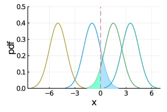
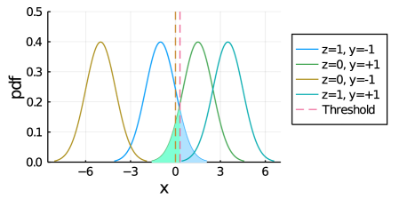
Figure 1: A toy example to interpret the influence scores of fairness. Left: The optimal classifier is $\bm{1}[x\geq 0]$. Four curves in different colors represent the distributions for each $(z,y)$ combination. The blue area and green area represent the violation of demographic parity. The data examples with low influence scores of fairness constraints are around $x=0$. Right: When we down-weight the examples around $x=0$, the optimal classifier will be perturbed towards right. Since the sum of blue area and green area decreases, the violation of demographic parity is mitigated.

4.3 Information Theoretic Algorithms

The demographic parity constraint can be interpreted as the independence of prediction $f(x)$ and group membership $z$. Denoted by $I(f(x);z)$ the mutual information between $f(x)$ and $z$, the independence condition $f(x)\perp\!\!\!\perp z$ implies $I(f(x);z)=0$. In consequence, a number of algorithms (Song et al., 2019; Gupta et al., 2021; Baharlouei et al., 2020) propose to adopt the bounds of mutual information $I(f(x);z)$ as the empirical fairness measure. We consider approximating mutual information by MINE (Belghazi et al., 2018; van den Oord et al., 2018) as an example.

$$\hat{\phi}(f)=\frac{1}{n}\sum_{i=1}^{n}\log\frac{\exp g(f(x_{i}),z_{i})}{\frac{1}{n}\sum_{k=1}^{n}\exp g(f(x_{i}),z_{k})}$$ (31)

where the function $g(\cdot,\cdot)$ is parameterized by a neural network. In this case, $\hat{\phi}(f)$ satisfies the decomposability assumption by straightly taking

$$\hat{\phi}(f,i)=\log\frac{\exp g(f(x_{i}),z_{i})}{\frac{1}{n}\sum_{k=1}^{n}\exp g(f(x_{i}),z_{k})}$$ (32)

Although the denominator inside the logarithm in Equation 32 contains the sum over all the $z_{k}$ in the training set, we can always calculated the sum when we know the prior distribution of the categorical variable $z$. Taking the derivative of $\hat{\phi}(f,i)$, the influence of MINE constraint is given by

$$S_{\textsf{MINE}}(i,j) =\lambda\frac{\eta}{n}\Theta(x_{i},x_{j};{\bm{\theta}}_{0})\cdot\left.\partialderivative{\mathbf{G}}{w}\right|_{w=f(x_{i};{\bm{\theta}})}$$ (33)

$$\text{where}\quad\mathbf{G} =g(w,z_{i})-\frac{1}{n}\sum_{k=1}^{n}g(w,z_{k})$$

Connection to Covariance.

In a special case when $g(f(x;{\bm{\theta}}),z)=zf(x;{\bm{\theta}})$, we have $\partial_{f}g(f(x;{\bm{\theta}}),z)=z$. Substitute the partial derivative back into Equation 33, the influence of MINE reduces to the influence of covariance measure $\lambda\frac{\eta}{n}\alpha_{i}(z_{i}-\bar{z})\Theta(x_{i},x_{j};{\bm{\theta}}_{0})$. However, it is very likely that the influence scores of MINE and covariance are much different, due to the fact that the unknown function $g(f(x),z)$ is parameterized by neural networks in more generic applications.

5 Estimating the Aggregated Influence Score

In this section, we intend to discuss the expected influence of a training example on the whole data distribution. We will focus on the changes of empirical fairness constraints $\hat{\phi}(f)$ when a data point $(x_{i},y_{i},z_{i})$ is excluded in the training set or not. Suppose that $\hat{\phi}(f)$ satisfies the decomposability assumption. We define the realized influence score of a training example $i$ aggregated over the whole data distribution $\mathcal{D}$ as

$$\mathcal{S}(i):=\int_{(x_{j},y_{j},z_{j})\in\mathcal{D}}\partialderivative{\hat{\phi}(f,j)}{f}S(i,j)\,d\Pr(x_{j},y_{j},z_{j})$$ (34)

$\mathcal{S}(i)$ takes into account the change on $\hat{\phi}(f)$ by applying the first-order approximation again for each test point $j$. In practice, the model $f$ can only observe finite data examples in $D$ that are drawn from the underlying distribution $\mathcal{D}$. We estimate the influence score of a training example $i$ over the training set $D$.

$$S(i):=\frac{1}{n}\sum_{i=1}^{n}\partialderivative{\hat{\phi}(f,j)}{f}S(i,j)$$ (35)

We wonder how the measure of $S(i)$ deviates from $\mathcal{S}(i)$.

Theorem 5.1 (Generalization Bound).

With probability at least $1-\epsilon$,

$$\mathcal{S}(i)-S(i)\leq\mathcal{O}\left(\sqrt{\frac{\log\frac{1}{\epsilon}}{2n}}\right)$$ (36)

Interpreting Influence Scores on Synthetic Data.

We consider a synthetic example as visualized in Figure 1 to illustrate why our influence scores help with identifying instances that affect the fairness. We assume that the individual examples are independently drawn from an underlying normal distribution corresponding to the label $y\in\{-1,+1\}$ and group membership $z\in\{0,1\}$, i.e., $x_{z,y}\sim N(\mu_{z,y},\sigma)$. We assume that $\mu_{0,-1}<\mu_{1,-1}<0<\mu_{0,+1}<\mu_{1,+1}$. Suppose that we train a linear model $f(x)=w\cdot x+b$, and the obtained classifier is $\bm{1}[f(x)>=0]$ which reduces to $\bm{1}[x>=0]$ for our toy example. Then we have the following proposition:

Proposition 5.2.

In our considered setting, if we down-weight the training examples with smaller absolute fairness influence scores, the model will tend to mitigate the violation of demographic parity.

Proposition 5.2 informs us that we can mitigate the unfairness by up-weighting the data instances with higher influence scores, or equivalently by removing some low-influence training points.

6 Evaluations

In this section, we examine the influence score subject to parity constraints on three different application domains: tabular data, images and natural language.

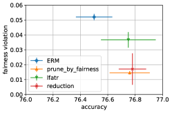
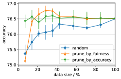
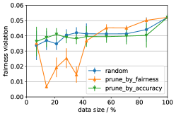
Figure 2: Results on Adult dataset. Figure 2: we benchmark the fairness and accuracy metrics for the baselines. Figure 2 and Figure 2: we compare how the proportion of unpruned training data affect the accuracy and fairness violation, respectively.

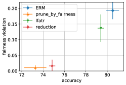
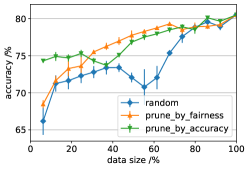
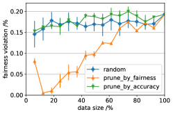
Figure 3: Results on CelebA dataset. Figure 3: we benchmark the fairness and accuracy metrics for the baselines. Figure 3 and Figure 3: we compare how the proportion of unpruned training data affect the accuracy and fairness violation, respectively.

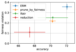
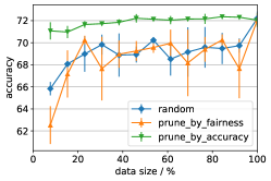
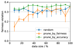
Figure 4: Results on Jigsaw dataset. Figure 4: we benchmark the fairness and accuracy metrics for the baselines. Figure 4 and Figure 4: we compare how the proportion of unpruned training data affect the accuracy and fairness violation, respectively.

6.1 Setup

We adopt the evaluation protocol that has been widely used by the previous papers on interpreting the impact of data examples. The basic idea is to train a model on a subset of training data by removing the less influential examples (Paul et al., 2021). In particular, we assess the performance of three data prune strategies: (1) random, which randomly selects a subset of training examples; (2) prune by fairness, which removes the data examples in the ascending order of the absolute values of aggregated influence scores subject to fairness as described in Equation 35; (3) prune by accuracy, which removes the data examples in the descending order of absolute influence scores in terms of the loss. The influence score is equivalent to the first order approximate proposed in (Pruthi et al., 2020). For the three strategies above, a model pre-trained on the whole training set will be used to estimate the influence scores of training examples with the direct application of Equation 35. We then execute the data prune procedure and impose the relaxed demographic parity in Equation 14 to train a fair model.

We compare the performance of pruning by influence scores with following optimization algorithms that regularize the constraint:

• ERM, which trains the model directly without imposing fairness constraints.

• lfatr (Madras et al., 2018), which regularizes the model with relaxed constraint as given in Equation 4.1.

• reduction (Agarwal et al., 2018), which reduces the constrained optimization to a cost-sensitive learning problem.

We used the Adam optimizer with a learning rate of 0.001 to train all the models. We used $\gamma=1$ for models requiring the regularizer parameter of fairness constraints. Any other hyperparameters keep the same among the compared methods. We report two metrics: the accuracy evaluated on test set and the difference of acceptance rates between groups as fairness violation. We defer more experimental details to Appendix C.

6.2 Result on Tabular Data

Firstly, we work with multi-layer perceptron (MLP) trained on the Adult dataset (Dua & Graff, 2017). We select sex, including female and male, as the sensitive attribute. We resample the dataset to balance the class and group membership. The MLP model is a two-layer ReLU network with hidden size 64. We train the model 5 times with different random seeds to report the mean and standard deviation of accuracy and fairness metrics. In each trial, the dataset is randomly split into a training and a test set in a ratio of 80 to 20. We compare the performance of prune by fairness in Figure 2 and find it has a similar fairness-accuracy trade-off with the reduction approach. To gain further insights, we plot how the size of pruned training examples affects the accuracy and fairness metrics for three prune strategies in Figure 2 and Figure 2. Not surprisingly, the random baseline remains a high fairness violation with a large accuracy drop when the data size decreases. In contrast, prune by fairness has a similar accuracy with pruning by accuracy when the data size is greater than $20\%$ and mitigates the fairness violation by a large margin when the data size is less than $40\%$. We also notice that prune by fairness anomalously has a high fairness violation when the data size is less than $10\%$. We conjecture such a small size of training data does not contain sufficient information, leading to the significant performance degradation. These observations suggest that we may obtain the best trade-off with a subset of only $20\%$–$40\%$ of training data.

6.3 Result on Images

Next, we train a ResNet-18 network (He et al., 2015) on the CelebA face attribute dataset (Liu et al., 2015). We select smiling as binary classification target and gender as the sensitive attribute. Figure 3 shows the trade-off between accuracy and fairness violation for each baseline method. We explore how the size of pruned training examples affects the accuracy and fairness metrics in Figure 3 and Figure 3. Again, the accuracy of prune by fairness has a similar trend with that of prune by accuracy when data size is larger than $20\%$, but drops strikingly with much smaller data size. On the other hand, prune by fairness mitigates the fairness violation straightly when data size decreases.

6.4 Result on Natural Language

Lastly, we consider Jigsaw Comment Toxicity Classification (Jigsaw, 2018) with text data. We select race as the sensitive attribute in our evaluation. We use pre-trained BERT (Devlin et al., 2019) to encode each raw comment text into a $768$-dimensional textual representation vector and train a two-layer neural network to perform classification. We report the experimental result in Figure 4. Figure 4 shows that prune by fairness has a mimic performance with lfatr while preserving smaller standard deviation. Figure 4 shows that prune by accuracy keeps a relatively high accuracy when a large subset of training examples are removed. In comparison, both prune by fairness and random prune failed to make informative prediction when the data size is below $20\%$. Figure 4 implies that prune by fairness is capable of mitigating bias. This result cautions that we need to carefully account for the price of a fair classifier, particularly in this application domain.

7 Conclusion

In this work, we have characterized the influence function subject to fairness constraints, which measures the change of model prediction on a target test point when a counterfactual training example is removed. We hope this work can inspire meaningful discussion regarding the impact of fairness constraints on individual examples. We propose exploring reasonable interpretations along this direction in real-world studies for future work.

Appendix A Impact of Fairness Constraints on Loss

We may also track the change in the test loss for a particular test point $x_{j}$ when training on a counterfactual instance $x_{i}$. Analogous to Equation 3, we may define the influence function in terms of the change of loss by

$$\text{infl}_{\ell}(D,i,j)\coloneqq\ell(f^{D/\{i\}}(x_{j}),y_{j})-\ell(f^{D}(x_{j};{\bm{\theta}},y_{j})$$ (37)

In the same way, we may approximate the influence with Taylor expansion again,

$$\text{infl}_{\ell}(D,i,j) =\ell(f(x_{j};{\bm{\theta}},y_{j})-\ell(f(x_{j};{\bm{\theta}}_{0}),y_{j})$$ (by Definition)

$$\approx\left.\frac{\partial\ell(w,y_{j})}{\partial w}\right|_{w=f(x_{j};{\bm{\theta}})}\left(f(x_{j};{\bm{\theta}})-f(x_{j};{\bm{\theta}}_{0})\right)$$ (by first-order Taylor expansion)

$$\approx\frac{\eta}{n}\left.\frac{\partial\ell(w,y_{j})}{\partial w}\right|_{w=f(x_{j};{\bm{\theta}}_{0})}\Theta(x_{i},x_{j};{\bm{\theta}}_{0})\left.\frac{\partial\ell(w,y_{i})}{\partial w}\right|_{w=f(x_{i};{\bm{\theta}}_{0})}$$ (by substituting Equation 8)

In more complicated situation where the fairness constraints are regularized, the influence function would be

$$\text{infl}_{\ell}(D,i,j) =\ell(f(x_{j};{\bm{\theta}},y_{j})-\ell(f(x_{j};{\bm{\theta}}_{0}),y_{j})$$

$$\approx\left.\frac{\partial\ell(w,y_{j})}{\partial w}\right|_{w=f(x_{j};{\bm{\theta}}_{0})}(f(x_{j};{\bm{\theta}})-f(x_{j};{\bm{\theta}}_{0}))$$

$$\approx\frac{\eta}{n}\left.\frac{\partial\ell(w,y_{j})}{\partial w}\right|_{w=f(x_{j};{\bm{\theta}}_{0})}\Theta(x_{i},x_{j};{\bm{\theta}}_{0})\left(\left.\frac{\partial\ell(w,y_{i})}{\partial w}\right|_{w=f(x_{i};{\bm{\theta}}_{0})}+\lambda\left.\frac{\partial\hat{\phi}(f,i)}{\partial f}\right|_{f(x_{i};{\bm{\theta}}_{0})}\right)$$ (38)

Equation A implies the intrinsic tension between accuracy and fairness — when the sign of $\partialderivative*{\ell(f(x_{i}),y_{i})}{f}$ are opposed to that of $\partialderivative*{\hat{\phi}(f,i)}{f}$, the influence of parity constraint will contradict with that of loss.

Appendix B Omitted Proofs

Proof of Corollary 4.1:

Proof.

Without loss of generality, we assume group $z=1$ has higher utilities than group $z=0$, i.e.,

$$\mathbb{E}[f(x;{\bm{\theta}})\bm{1}[z=1,y=1]] \geq\mathbb{E}[f(x;{\bm{\theta}})\bm{1}[z=0,y=1]]$$

$$\mathbb{E}[f(x;{\bm{\theta}})\bm{1}[z=1,y=0]] \geq\mathbb{E}[f(x;{\bm{\theta}})\bm{1}[z=0,y=0]]$$

Equal odds indicates equal TPR and equal FPR constraints will be imposed simultaneously. Thereby

$$S_{\textsf{EO}} =S_{\textsf{TPR}}+S_{\textsf{FPR}}$$

$$=\lambda\frac{\eta}{n}\alpha_{z_{i},y_{i}}\Theta(x_{i},x_{j};{\bm{\theta}}_{0})+\lambda\frac{\eta}{n}\tilde{\alpha}_{z_{i},y_{i}}\Theta(x_{i},x_{j};{\bm{\theta}}_{0})$$

$$=\lambda\frac{\eta}{n}\alpha_{z_{i}}\Theta(x_{i},x_{j};{\bm{\theta}}_{0}) \alpha_{z}=\alpha_{z,y}+\tilde{\alpha}_{z,y}$$ (by )

$$=S_{\textsf{DP}}$$

The third equality is due to $\alpha_{z}=\bm{1}[z=1]-\bm{1}[z=0]=(\bm{1}[z=1,y=+1]+\bm{1}[z=1,y=-1])-(\bm{1}[z=0,y=+1]+\bm{1}[z=0,y=-1])=\alpha_{z,y}+\tilde{\alpha}_{z,y}$. ∎

Proof of Corollary 4.2:

Proof.

When there are only two groups, the covariance measure in Equation 27 reduces to

$$\hat{\phi}(f)=|\frac{1}{n}\sum_{i=1}^{n}(z_{i}-\frac{1}{2})f(x_{i};{\bm{\theta}})|$$

Again, we assume group $z=1$ is more favorable than group $z=0$ such that $\mathbb{E}[f(x;{\bm{\theta}})\bm{1}[z=1]]\geq\mathbb{E}[f(x;{\bm{\theta}})\bm{1}[z=0]]$. Then we can rewrite the above equation as

$$\hat{\phi}(f) =\frac{1}{n}\sum_{i=1}^{n}\frac{1}{2}f(x_{i};{\bm{\theta}})\bm{1}[z_{i}=1]-\frac{1}{n}\sum_{i=1}^{n}\frac{1}{2}f(x_{i};{\bm{\theta}})\bm{1}[z_{i}=0])\geq 0$$

The above $\hat{\phi}(f)$ is saying the covariance between $z$ and $f(x)$ is non-negative per se, so we do not need to take the absolute value of it. In other words, $\forall i,\beta_{i}=1$. The final influence score of covariance thus becomes

$$S_{\textsf{cov}}(i,j)=\lambda\frac{\eta}{2n}\Theta(x_{i},x_{j};{\bm{\theta}}_{0})(\bm{1}[z_{i}=1]-\bm{1}[z_{i}=0])$$

Recall that $\alpha_{i}=\bm{1}[z_{i}=1]-\bm{1}[z_{i}=0]$, we conclude $S_{\textsf{cov}}(i,j)=\frac{1}{2}S_{\textsf{DP}}(i,j)$. We note that the connection builds upon the common assumption that group $z=1$ has a higher utility. We can reach the same conclusion in the symmetric situation where $\mathbb{E}[f(x;{\bm{\theta}})\bm{1}[z=1]]<\mathbb{E}[f(x;{\bm{\theta}})\bm{1}[z=0]]$.

We remark, the coefficient $\frac{1}{2}$ arises from encoding the categorical sensitive variable $z$ into $\{0,1\}$ and does not have physical meanings. If $z$ is encoded by $\{-1,+1\}$ instead, the coefficient will be $1$ such that $S_{\textsf{DP}}=S_{\textsf{cov}}$. This property suggests that the covariance is not a perfect measure of independence, and using mutual information is a more plausible approach. ∎

Proof of Theorem 5.1

Proof.

For any $t$ and any $\delta>0$,

$$\Pr(\mathcal{S}(f,j)-S(f,j)>\delta) =\Pr(\exp{nt\left(\mathcal{S}(f,j)-S(f,j)\right)}>\exp{nt\delta})$$

$$\leq\frac{\mathbb{E}[\exp{nt(\mathcal{S}(f,j)-S(f,j))}]}{\exp{nt\delta}}$$ (by Markov’s inequality)

$$\leq\exp{\frac{1}{8}nt^{2}C^{2}-nt\delta}$$ (by Hoeffding’s inequality)

In above $C$ is some constant. Since $\frac{1}{8}nC^{2}t^{2}-n\delta t$ is a quadratic function regarding $t$, we may minimize it by taking

$$\partialderivative{t}(\frac{1}{8}nC^{2}t^{2}-n\delta t)=0\implies\frac{1}{4}nC^{2}t-n\delta t=0$$

Solving the above equation, we know the quadratic function takes the minimum value at $t=\frac{\delta}{4C^{2}}$. Therefore,

$$\Pr\left(\mathcal{S}(f,j)-S(f,j)>\delta\right)\leq\exp{-\frac{2n\delta^{2}}{C^{2}}}$$

Let $\epsilon=\exp{-\frac{2n\delta^{2}}{C^{2}}}$, we complete the proof by substituting $\delta$ with $\epsilon$

$$\Pr\left(\mathcal{S}(f,j)-S(f,j)>C\sqrt{\frac{\log\frac{1}{\epsilon}}{2n}}~{}\right)\leq\epsilon\implies\Pr\left(\mathcal{S}(f,j)-S(f,j)\leq C\sqrt{\frac{\log\frac{1}{\epsilon}}{2n}}~{}\right)>1-\epsilon$$

∎

Proof of Proposition 5.2

Proof.

We visualize the considered example in Figure 1. The area in blue represents the false positive examples from group $z=1$, while the area in green represents the false negative examples from group $z=0$. The sum of blue area and green area is exactly representing the acceptance rate difference between group $z=1$ and $z=0$.

Recall that the model is $f(x)=w\cdot x+b$, the influence function subject to relaxed fairness constraint can be computed by Equation 17, i.e., $S(i,j)=k(z_{i}-\bar{z})\cdot(x_{i}\cdot x_{j}+1)$ where $k$ is a constant coefficient corresponding to learning rate $\eta$, data size $n$ and regularizer $\lambda$. For each individual example $x_{i}$, the overall influence score $S(i)$ consists of two components. The first component

$$\int_{x_{j}\in(-\infty,+\infty)}k(z_{j}-\bar{z})\cdot(z_{i}-\bar{z})\cdot x_{i}\cdot x_{j}\,d\Pr(x_{j})=k(z_{i}-\bar{z})x_{i}\cdot\int_{x_{j}\in(-\infty,+\infty)}(z_{j}-\bar{z})\cdot x_{j}\,d\Pr(x_{j})$$

is proportional to $(z_{i}-\bar{z})x_{i}$ since the integral can be treated as a constant. The second component

$$\int_{x_{j}\in(-\infty,+\infty)}k(z_{j}-\bar{z})\cdot(z_{i}-\bar{z})\,d\Pr(x_{j})=k(z_{i}-\bar{z})\cdot\int_{x_{j}\in(-\infty,+\infty)}(z_{j}-\bar{z})\,d\Pr(x_{j})=k(z_{i}-\bar{z})\mathbb{E}[z_{j}-\bar{z}]$$

becomes $0$ due to $\mathbb{E}[z_{j}]=\bar{z}$ . $|S(i)|$ is then proportional to $|x_{i}|$, thus the data examples around $x=0$ will have smaller absolute values of influence scores.

Then we consider the classifier trained by down-weighting the data examples around $x=0$. We show the case when $|\mu_{1,-1}|<|\mu_{0,+1}|$ in the right figure in Figure 1. In this case, the down-weighted negative examples from group $z=1$ dominates the down-weighted positive examples from group $z=0$. In consequence, the decision threshold will be perturbed towards right. Coloring the mis-classified examples again, we find out the sum of blue and green area has decreased. The case for $|\mu_{1,-1}|<|\mu_{0,+1}|$ will be symmetric. In conclusion, we demonstrate that removing training examples with smaller absolute influence scores is capable of mitigating the fairness violation. ∎

Appendix C Additional Experimental Results

C.1 Computing Infrastructure

For all the experiments, we use a GPU cluster with four NVIDIA RTX A6000 GPUs for training and evaluation. We observe that it is efficient to compute the first-order approximated influence scores. It took less than 10 minutes to compute the influence scores for the training examples in CelebA dataset and cost about $0.01$ kg of CO2 equivalent carbon emission.

C.2 Experimental Details

Details on Adult dataset

The UCI Adult (Dua & Graff, 2017) is a census-based dataset for predicting whether an individual’s annual income is greater than 50K, consisting of $14$ features and $48,842$ instances. We select sex, including female and male, as the sensitive attribute. We resample the dataset to balance the class and group membership. The MLP model is a two-layer ReLU network with a hidden size of 64. We train the model 5 times with different random seeds to report the mean and standard deviation of accuracy and fairness metrics. In each trial, the dataset is randomly split into a training and a test set in a ratio of 80 to 20.

Details on CelebA dataset

The CelebA dataset contains 202,599 face images, where each image is associated with 40 binary human-labeled attributes. We select smiling as binary classification target and gender as the sensitive attribute. We train a ResNet-18 (He et al., 2015) along with two fully-connected layers for prediction. We follow the original train test splits. We repeat 5 times with different random seeds to report the mean and standard deviation.

Details on Jigsaw dataset

Jigsaw Comment Toxicity Classification (Jigsaw, 2018) was initially released as a Kaggle public competition. The task is to build a model that recognizes toxic comments and minimizes the unintended bias with respect to mentions of sensitive identities, including gender and race. We select race as the sensitive attribute in our evaluation. Since only a subset provides sensitive identity annotations, we drop the entries with missing race values. We use pre-trained BERT (Devlin et al., 2019) to encode each raw comment text into a $768$-dimensional textual representation vector. Then we train a two-layer neural network to perform classification with the encoded textual features. We use the official train set for training and the expanded public test set for testing.

C.3 Effect of First Order Approximation

To understand the effect of first order approximation, we train a two-layer neural network with hidden size 64 on the Adult dataset. We randomly pick $1,000$ pairs of training and test points. Upon updating the parameters corresponding to the training point, we calculate the difference of model output on the test point. We directly apply Equation 11 to estimate the influence. Figure 5 compares how well does the approximated influence align with the real change on model prediction. We find out that the correlation between the two quantities is, without doubt, very closed to 1.

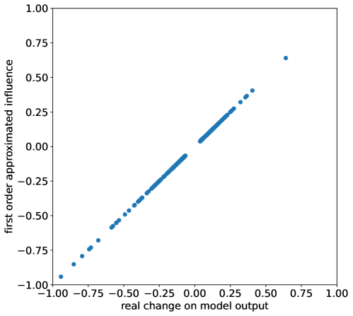
Figure 5: We compare the real change on model output and the pairwise influence with first order approximation.

C.4 Detecting Influential Examples

It is intriguing to figure out which examples have the highest and lowest influence scores regarding fairness. On the CelebA dataset, we rank the facial images based on their influence scores by Equation 35. We extract 20 images with highest scores and 20 images with lowest scores, and compare their group distribution in Figure 6(b). We observe that the group distribution is rather balanced for high influence examples, with 9 men and 11 women. However, the group distribution is tremendously skewed towards the male group than the female group, with 17 men and only 3 women. Comparing the accuracy rate for two groups in Figure 6(a), we conjecture this disparity arose from the lower accuracy for the male group (78.1%) than the female group (79.4%).

(a) Accuracy Gap

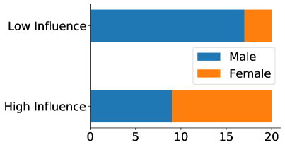
(b) Distribution Disparity

Figure 6: We observe that the extracted high influence examples are rather balanced, but the low influence examples are extremely unbalanced for the protected groups.

References

- Agarwal et al. (2018) Agarwal, A., Beygelzimer, A., Dudík, M., Langford, J., and Wallach, H. M. A reductions approach to fair classification. In Dy, J. G. and Krause, A. (eds.), ICML, volume 80 of Proceedings of Machine Learning Research, pp. 60–69. PMLR, 2018. URL http://proceedings.mlr.press/v80/agarwal18a.html.
- Ajunwa et al. (2016) Ajunwa, I., Friedler, S. A., Scheidegger, C. E., and Venkatasubramanian, S. Hiring by algorithm: Predicting and preventing disparate impact. In the Yale Law School Information Society Project conference Unlocking the Black Box: The Promise and Limits of Algorithmic Accountability in the Professions, April 2016.
- Angwin et al. (2016) Angwin, J., Larson, J., Mattu, S., and Kirchner, L. Machine Bias, 2016.
- Baharlouei et al. (2020) Baharlouei, S., Nouiehed, M., Beirami, A., and Razaviyayn, M. Rényi fair inference. In International Conference on Learning Representations, 2020. URL https://openreview.net/forum?id=HkgsUJrtDB.
- Balcan et al. (2019) Balcan, M.-F. F., Dick, T., Noothigattu, R., and Procaccia, A. D. Envy-free classification. In Wallach, H., Larochelle, H., Beygelzimer, A., d'Alché-Buc, F., Fox, E., and Garnett, R. (eds.), Advances in Neural Information Processing Systems, volume 32. Curran Associates, Inc., 2019. URL https://proceedings.neurips.cc/paper/2019/file/e94550c93cd70fe748e6982b3439ad3b-Paper.pdf.
- Basu et al. (2020) Basu, S., You, X., and Feizi, S. On second-order group influence functions for black-box predictions. In Proceedings of the 37th International Conference on Machine Learning, ICML 2020, 13-18 July 2020, Virtual Event, volume 119 of Proceedings of Machine Learning Research, pp. 715–724. PMLR, 2020. URL http://proceedings.mlr.press/v119/basu20b.html.
- Basu et al. (2021) Basu, S., Pope, P., and Feizi, S. Influence functions in deep learning are fragile. In International Conference on Learning Representations, 2021. URL https://openreview.net/forum?id=xHKVVHGDOEk.
- Belghazi et al. (2018) Belghazi, M. I., Baratin, A., Rajeshwar, S., Ozair, S., Bengio, Y., Courville, A., and Hjelm, D. Mutual information neural estimation. In Dy, J. and Krause, A. (eds.), Proceedings of the 35th International Conference on Machine Learning, volume 80 of Proceedings of Machine Learning Research, pp. 531–540. PMLR, 10–15 Jul 2018. URL https://proceedings.mlr.press/v80/belghazi18a.html.
- Black & Fredrikson (2021) Black, E. and Fredrikson, M. Leave-one-out unfairness. In Proceedings of the 2021 ACM Conference on Fairness, Accountability, and Transparency, FAccT ’21, pp. 285–295, New York, NY, USA, 2021. Association for Computing Machinery. ISBN 9781450383097. doi: 10.1145/3442188.3445894. URL https://doi.org/10.1145/3442188.3445894.
- Bogen & Rieke (2018) Bogen, M. and Rieke, A. Help wanted: an examination of hiring algorithms, equity, and bias. Technical report, Upturn, 2018. URL https://www.upturn.org/static/reports/2018/hiring-algorithms/files/Upturn%20--%20Help%20Wanted%20-%20An%20Exploration%20of%20Hiring%20Algorithms,%20Equity%20and%20Bias.pdf.
- Bolukbasi et al. (2016) Bolukbasi, T., Chang, K.-W., Zou, J., Saligrama, V., and Kalai, A. Man is to computer programmer as woman is to homemaker? debiasing word embeddings. In Proceedings of the 30th International Conference on Neural Information Processing Systems, NIPS’16, pp. 4356–4364, Red Hook, NY, USA, 2016. Curran Associates Inc. ISBN 9781510838819.
- Brunet et al. (2019) Brunet, M.-E., Alkalay-Houlihan, C., Anderson, A., and Zemel, R. Understanding the origins of bias in word embeddings. In Chaudhuri, K. and Salakhutdinov, R. (eds.), Proceedings of the 36th International Conference on Machine Learning, volume 97 of Proceedings of Machine Learning Research, pp. 803–811. PMLR, 09–15 Jun 2019. URL https://proceedings.mlr.press/v97/brunet19a.html.
- Buolamwini & Gebru (2018) Buolamwini, J. and Gebru, T. Gender shades: Intersectional accuracy disparities in commercial gender classification. In Friedler, S. A. and Wilson, C. (eds.), Proceedings of the 1st Conference on Fairness, Accountability and Transparency, volume 81 of Proceedings of Machine Learning Research, pp. 77–91. PMLR, 23–24 Feb 2018. URL https://proceedings.mlr.press/v81/buolamwini18a.html.
- Calmon et al. (2017) Calmon, F., Wei, D., Vinzamuri, B., Natesan Ramamurthy, K., and Varshney, K. R. Optimized pre-processing for discrimination prevention. In Guyon, I., Luxburg, U. V., Bengio, S., Wallach, H., Fergus, R., Vishwanathan, S., and Garnett, R. (eds.), Advances in Neural Information Processing Systems 30, pp. 3992–4001. Curran Associates, Inc., 2017. URL http://papers.nips.cc/paper/6988-optimized-pre-processing-for-discrimination-prevention.pdf.
- Chouldechova (2017) Chouldechova, A. Fair prediction with disparate impact: A study of bias in recidivism prediction instruments. Big data, 5 2:153–163, 2017.
- Chuang & Mroueh (2021) Chuang, C.-Y. and Mroueh, Y. Fair mixup: Fairness via interpolation. In International Conference on Learning Representations, 2021. URL https://openreview.net/forum?id=DNl5s5BXeBn.
- Cook & Weisberg (1980) Cook, R. D. and Weisberg, S. Characterizations of an empirical influence function for detecting influential cases in regression. Technometrics, 22:495–508, 1980.
- Corbett-Davies et al. (2017) Corbett-Davies, S., Pierson, E., Feller, A., Goel, S., and Huq, A. Algorithmic decision making and the cost of fairness. In Proceedings of the 23rd acm sigkdd international conference on knowledge discovery and data mining, pp. 797–806, 2017.
- Cotter et al. (2019a) Cotter, A., Jiang, H., and Sridharan, K. Two-player games for efficient non-convex constrained optimization. In ALT, 2019a.
- Cotter et al. (2019b) Cotter, A., Jiang, H., Wang, S., Narayan, T., Gupta, M., You, S., and Sridharan, K. Optimization with non-differentiable constraints with applications to fairness, recall, churn, and other goals. ArXiv, abs/1809.04198, 2019b.
- Devlin et al. (2019) Devlin, J., Chang, M.-W., Lee, K., and Toutanova, K. BERT: Pre-training of deep bidirectional transformers for language understanding. In Proceedings of the 2019 Conference of the North American Chapter of the Association for Computational Linguistics: Human Language Technologies, Volume 1 (Long and Short Papers), pp. 4171–4186, Minneapolis, Minnesota, June 2019. Association for Computational Linguistics. doi: 10.18653/v1/N19-1423. URL https://aclanthology.org/N19-1423.
- Dieterich et al. (2016) Dieterich, W., Mendoza, C., and Brennan, T. Compas risk scales : Demonstrating accuracy equity and predictive parity performance of the compas risk scales in broward county. Technical report, Northpointe Inc., July 2016.
- Dua & Graff (2017) Dua, D. and Graff, C. UCI machine learning repository, 2017. URL http://archive.ics.uci.edu/ml.
- Dwork et al. (2012) Dwork, C., Hardt, M., Pitassi, T., Reingold, O., and Zemel, R. Fairness through awareness. In Proceedings of the 3rd innovations in theoretical computer science conference, pp. 214–226, 2012.
- Feldman et al. (2015) Feldman, M., Friedler, S. A., Moeller, J., Scheidegger, C., and Venkatasubramanian, S. Certifying and removing disparate impact. In Proceedings of the 21th ACM SIGKDD International Conference on Knowledge Discovery and Data Mining, KDD ’15, pp. 259–268, New York, NY, USA, 2015. Association for Computing Machinery. ISBN 9781450336642. doi: 10.1145/2783258.2783311. URL https://doi.org/10.1145/2783258.2783311.
- Feldman (2020) Feldman, V. Does learning require memorization? a short tale about a long tail. Proceedings of the 52nd Annual ACM SIGACT Symposium on Theory of Computing, 2020.
- Feldman & Zhang (2020) Feldman, V. and Zhang, C. What neural networks memorize and why: Discovering the long tail via influence estimation. In Larochelle, H., Ranzato, M., Hadsell, R., Balcan, M. F., and Lin, H. (eds.), Advances in Neural Information Processing Systems, volume 33, pp. 2881–2891. Curran Associates, Inc., 2020. URL https://proceedings.neurips.cc/paper/2020/file/1e14bfe2714193e7af5abc64ecbd6b46-Paper.pdf.
- Gupta et al. (2021) Gupta, U., Ferber, A., Dilkina, B. N., and Steeg, G. V. Controllable guarantees for fair outcomes via contrastive information estimation. In AAAI, 2021.
- Hardt et al. (2016) Hardt, M., Price, E., and Srebro, N. Equality of opportunity in supervised learning. In Proceedings of the 30th International Conference on Neural Information Processing Systems, NIPS’16, pp. 3323–3331, Red Hook, NY, USA, 2016. Curran Associates Inc. ISBN 9781510838819.
- He et al. (2015) He, K., Zhang, X., Ren, S., and Sun, J. Deep residual learning for image recognition. CoRR, abs/1512.03385, 2015. URL http://arxiv.org/abs/1512.03385.
- Jacot et al. (2018) Jacot, A., Gabriel, F., and Hongler, C. Neural tangent kernel: Convergence and generalization in neural networks. In Bengio, S., Wallach, H., Larochelle, H., Grauman, K., Cesa-Bianchi, N., and Garnett, R. (eds.), Advances in Neural Information Processing Systems, volume 31. Curran Associates, Inc., 2018. URL https://proceedings.neurips.cc/paper/2018/file/5a4be1fa34e62bb8a6ec6b91d2462f5a-Paper.pdf.
- Jiang et al. (2022) Jiang, Z., Han, X., Fan, C., Yang, F., Mostafavi, A., and Hu, X. Generalized demographic parity for group fairness. In International Conference on Learning Representations, 2022. URL https://openreview.net/forum?id=YigKlMJwjye.
- Jigsaw (2018) Jigsaw. Jigsaw unintended bias in toxicity classification, 2018. URL https://www.kaggle.com/c/jigsaw-unintended-bias-in-toxicity-classification.
- KamiranFaisal & CaldersToon (2012) KamiranFaisal and CaldersToon. Data preprocessing techniques for classification without discrimination. Knowledge and Information Systems, 2012.
- Kamishima et al. (2011) Kamishima, T., Akaho, S., and Sakuma, J. Fairness-aware learning through regularization approach. 2011 IEEE 11th International Conference on Data Mining Workshops, pp. 643–650, 2011.
- Koh & Liang (2017) Koh, P. W. and Liang, P. Understanding black-box predictions via influence functions. In Precup, D. and Teh, Y. W. (eds.), Proceedings of the 34th International Conference on Machine Learning, volume 70 of Proceedings of Machine Learning Research, pp. 1885–1894. PMLR, 06–11 Aug 2017. URL https://proceedings.mlr.press/v70/koh17a.html.
- Koh et al. (2018) Koh, P. W., Steinhardt, J., and Liang, P. Stronger data poisoning attacks break data sanitization defenses. CoRR, abs/1811.00741, 2018. URL http://arxiv.org/abs/1811.00741.
- Kusner et al. (2017a) Kusner, M. J., Loftus, J., Russell, C., and Silva, R. Counterfactual fairness. In Guyon, I., Luxburg, U. V., Bengio, S., Wallach, H., Fergus, R., Vishwanathan, S., and Garnett, R. (eds.), Advances in Neural Information Processing Systems, volume 30. Curran Associates, Inc., 2017a. URL https://proceedings.neurips.cc/paper/2017/file/a486cd07e4ac3d270571622f4f316ec5-Paper.pdf.
- Kusner et al. (2017b) Kusner, M. J., Loftus, J., Russell, C., and Silva, R. Counterfactual fairness. In Guyon, I., Luxburg, U. V., Bengio, S., Wallach, H., Fergus, R., Vishwanathan, S., and Garnett, R. (eds.), Advances in Neural Information Processing Systems, volume 30. Curran Associates, Inc., 2017b. URL https://proceedings.neurips.cc/paper/2017/file/a486cd07e4ac3d270571622f4f316ec5-Paper.pdf.
- Liu & Wang (2021) Liu, Y. and Wang, J. Can less be more? when increasing-to-balancing label noise rates considered beneficial. In Beygelzimer, A., Dauphin, Y., Liang, P., and Vaughan, J. W. (eds.), Advances in Neural Information Processing Systems, 2021. URL https://openreview.net/forum?id=VjKhSULF7Gb.
- Liu et al. (2015) Liu, Z., Luo, P., Wang, X., and Tang, X. Deep learning face attributes in the wild. In Proceedings of International Conference on Computer Vision (ICCV), December 2015.
- Lundberg & Lee (2017) Lundberg, S. M. and Lee, S.-I. A unified approach to interpreting model predictions. In Guyon, I., Luxburg, U. V., Bengio, S., Wallach, H., Fergus, R., Vishwanathan, S., and Garnett, R. (eds.), Advances in Neural Information Processing Systems, volume 30. Curran Associates, Inc., 2017. URL https://proceedings.neurips.cc/paper/2017/file/8a20a8621978632d76c43dfd28b67767-Paper.pdf.
- Madras et al. (2018) Madras, D., Creager, E., Pitassi, T., and Zemel, R. S. Learning adversarially fair and transferable representations. CoRR, abs/1802.06309, 2018. URL http://arxiv.org/abs/1802.06309.
- Mase et al. (2021) Mase, M., Owen, A. B., and Seiler, B. B. Cohort shapley value for algorithmic fairness. ArXiv, abs/2105.07168, 2021.
- Mayson (2019) Mayson, S. G. Bias in, bias out. Yale Law Journal, 128(8):2218, June 2019.
- Mitchell et al. (2019) Mitchell, M., Wu, S., Zaldivar, A., Barnes, P., Vasserman, L., Hutchinson, B., Spitzer, E., Raji, I. D., and Gebru, T. Model cards for model reporting. In Proceedings of the Conference on Fairness, Accountability, and Transparency, FAT* ’19, pp. 220–229, New York, NY, USA, 2019. Association for Computing Machinery. ISBN 9781450361255. doi: 10.1145/3287560.3287596. URL https://doi.org/10.1145/3287560.3287596.
- Narasimhan (2018) Narasimhan, H. Learning with complex loss functions and constraints. In Storkey, A. and Perez-Cruz, F. (eds.), Proceedings of the Twenty-First International Conference on Artificial Intelligence and Statistics, volume 84 of Proceedings of Machine Learning Research, pp. 1646–1654. PMLR, 09–11 Apr 2018. URL https://proceedings.mlr.press/v84/narasimhan18a.html.
- Ninth Circuit Jury Instructions Committee (2017) Ninth Circuit Jury Instructions Committee. Manual of Model Civil Jury Instructions for the Ninth Circuit, chapter 11. St. Paul, Minn. :West Publishing, 2017. URL https://www.ce9.uscourts.gov/jury-instructions/model-civil.
- Paul et al. (2021) Paul, M., Ganguli, S., and Dziugaite, G. K. Deep learning on a data diet: Finding important examples early in training. In Beygelzimer, A., Dauphin, Y., Liang, P., and Vaughan, J. W. (eds.), Advances in Neural Information Processing Systems, 2021. URL https://openreview.net/forum?id=Uj7pF-D-YvT.
- Petersen et al. (2021) Petersen, F., Mukherjee, D., Sun, Y., and Yurochkin, M. Post-processing for individual fairness. In Beygelzimer, A., Dauphin, Y., Liang, P., and Vaughan, J. W. (eds.), Advances in Neural Information Processing Systems, 2021. URL https://openreview.net/forum?id=qGeqg4_hA2.
- Pfohl et al. (2021) Pfohl, S. R., Foryciarz, A., and Shah, N. H. An empirical characterization of fair machine learning for clinical risk prediction. Journal of biomedical informatics, pp. 103621, 2021.
- Pruthi et al. (2020) Pruthi, G., Liu, F., Kale, S., and Sundararajan, M. Estimating training data influence by tracing gradient descent. In Larochelle, H., Ranzato, M., Hadsell, R., Balcan, M. F., and Lin, H. (eds.), Advances in Neural Information Processing Systems, volume 33, pp. 19920–19930. Curran Associates, Inc., 2020. URL https://proceedings.neurips.cc/paper/2020/file/e6385d39ec9394f2f3a354d9d2b88eec-Paper.pdf.
- Raghavan et al. (2020) Raghavan, M., Barocas, S., Kleinberg, J., and Levy, K. Mitigating bias in algorithmic hiring: Evaluating claims and practices. In Proceedings of the 2020 Conference on Fairness, Accountability, and Transparency, FAT* ’20, pp. 469–481, New York, NY, USA, 2020. Association for Computing Machinery. ISBN 9781450369367. doi: 10.1145/3351095.3372828. URL https://doi.org/10.1145/3351095.3372828.
- Siddiqi (2005) Siddiqi, N. Credit Risk Scorecards: Developing and Implementing Intelligent Credit Scoring. Wiley, September 2005. ISBN 978-1-119-20173-1.
- Song et al. (2019) Song, J., Kalluri, P., Grover, A., Zhao, S., and Ermon, S. Learning controllable fair representations. In AISTATS, 2019.
- Sundararajan & Najmi (2020) Sundararajan, M. and Najmi, A. The many shapley values for model explanation. In III, H. D. and Singh, A. (eds.), Proceedings of the 37th International Conference on Machine Learning, volume 119 of Proceedings of Machine Learning Research, pp. 9269–9278. PMLR, 13–18 Jul 2020. URL https://proceedings.mlr.press/v119/sundararajan20b.html.
- Sundararajan et al. (2017) Sundararajan, M., Taly, A., and Yan, Q. Axiomatic attribution for deep networks. In Precup, D. and Teh, Y. W. (eds.), Proceedings of the 34th International Conference on Machine Learning, volume 70 of Proceedings of Machine Learning Research, pp. 3319–3328. PMLR, 06–11 Aug 2017. URL https://proceedings.mlr.press/v70/sundararajan17a.html.
- Taskesen et al. (2020) Taskesen, B., Nguyen, V. A., Kuhn, D., and Blanchet, J. H. A distributionally robust approach to fair classification. ArXiv, abs/2007.09530, 2020.
- Ustun et al. (2019) Ustun, B., Spangher, A., and Liu, Y. Actionable recourse in linear classification. In Proceedings of the Conference on Fairness, Accountability, and Transparency, FAT* ’19, pp. 10–19, New York, NY, USA, 2019. Association for Computing Machinery. ISBN 9781450361255. doi: 10.1145/3287560.3287566. URL https://doi.org/10.1145/3287560.3287566.
- van den Oord et al. (2018) van den Oord, A., Li, Y., and Vinyals, O. Representation learning with contrastive predictive coding. ArXiv, abs/1807.03748, 2018.
- Wang et al. (2021) Wang, J., Liu, Y., and Levy, C. Fair classification with group-dependent label noise. In Proceedings of the 2021 ACM Conference on Fairness, Accountability, and Transparency, FAccT ’21, pp. 526–536, New York, NY, USA, 2021. Association for Computing Machinery. ISBN 9781450383097. doi: 10.1145/3442188.3445915. URL https://doi.org/10.1145/3442188.3445915.
- Wang et al. (2022) Wang, J., Liu, Y., and Wang, X. Assessing multilingual fairness in pre-trained multimodal representations. In Findings of the Association for Computational Linguistics: ACL 2022, pp. 2681–2695, Dublin, Ireland, May 2022. Association for Computational Linguistics. doi: 10.18653/v1/2022.findings-acl.211. URL https://aclanthology.org/2022.findings-acl.211.
- Woodworth et al. (2017) Woodworth, B., Gunasekar, S., Ohannessian, M. I., and Srebro, N. Learning non-discriminatory predictors. In Kale, S. and Shamir, O. (eds.), Proceedings of the 2017 Conference on Learning Theory, volume 65 of Proceedings of Machine Learning Research, pp. 1920–1953. PMLR, 07–10 Jul 2017. URL https://proceedings.mlr.press/v65/woodworth17a.html.
- Zafar et al. (2017) Zafar, M., Valera, I., Gomez-Rodriguez, M., and Gummadi, K. Fairness constraints: Mechanisms for fair classification. In AISTATS, 2017.
- Zhou et al. (2021) Zhou, Y., Huang, S.-C., Fries, J. A., Youssef, A., Amrhein, T. J., Chang, M., Banerjee, I., Rubin, D., Xing, L., Shah, N., and Lungren, M. P. Radfusion: Benchmarking performance and fairness for multimodal pulmonary embolism detection from ct and ehr, 2021.
- Zhu et al. (2022a) Zhu, Z., Dong, Z., and Liu, Y. Detecting corrupted labels without training a model to predict. In Proceedings of the 39th International Conference on Machine Learning. PMLR, 2022a.
- Zhu et al. (2022b) Zhu, Z., Luo, T., and Liu, Y. The rich get richer: Disparate impact of semi-supervised learning. In International Conference on Learning Representations, 2022b. URL https://openreview.net/forum?id=DXPftn5kjQK.