A simple algorithm for expanding a power series
as a continued fraction

Abstract

I present and discuss an extremely simple algorithm for expanding a formal power series as a continued fraction. This algorithm, which goes back to Euler (1746) and Viscovatov (1805), deserves to be better known. I also discuss the connection of this algorithm with the work of Gauss (1812), Stieltjes (1889), Rogers (1907) and Ramanujan, and a combinatorial interpretation based on the work of Flajolet (1980).

Key Words: Formal power series, continued fraction, Euler–Viscovatov algorithm, Gauss’s continued fraction, Euler–Gauss recurrence method, Motzkin path, Dyck path, Stieltjes table, Rogers’ addition formula.

Mathematics Subject Classification (MSC 2010) codes: 30B70 (Primary); 05A10, 05A15, 05A19 (Secondary).

• Surely the story unfolded here emphasizes how valuable it is to study and understand the central ideas behind major pieces of mathematics produced by giants like Euler.

  — George Andrews [3, p. 284]

1 Introduction

The expansion of power series into continued fractions goes back nearly 300 years. Euler [41] showed circa 1746 that

$$\sum_{n=0}^{\infty}n!\>t^{n}\;=\;\cfrac{1}{1-\cfrac{1t}{1-\cfrac{1t}{1-\cfrac{2t}{1-\cfrac{2t}{1-\cfrac{3t}{1-\cfrac{3t}{1-\cdots}}}}}}}$$ (1.1)

and more generally that

$$\sum_{n=0}^{\infty}a(a+1)(a+2)\cdots(a+n-1)\>t^{n}\;=\;\cfrac{1}{1-\cfrac{at}{1-\cfrac{1t}{1-\cfrac{(a+1)t}{1-\cfrac{2t}{1-\cfrac{(a+2)t}{1-\cfrac{3t}{1-\cdots}}}}}}}\;\,.$$ (1.2)

Lambert [70] showed circa 1761 that

$${\tan t\over t}\;=\;\cfrac{1}{1-\cfrac{{1\over 1\cdot 3}t^{2}}{1-\cfrac{{1\over 3\cdot 5}t^{2}}{1-\cfrac{{1\over 5\cdot 7}t^{2}}{1-\cfrac{{1\over 7\cdot 9}t^{2}}{1-\cdots}}}}}$$ (1.3)

and used it to prove the irrationality of $\pi$ [68, 105]. Many similar expansions were discovered in the eighteenth and nineteenth centuries: most notably, Gauss [51] found in 1812 a continued-fraction expansion for the ratio of two contiguous hypergeometric functions ${{\tensor[_{2\!}]{F}{{}_{1}}\!}}$, from which many previously obtained expansions can be deduced by specialization or taking limits [104, Chapter XVIII]. A detailed history of continued fractions can be found in the fascinating book of Brezinski [22].

Let us stress that this subject has two facets: algebraic and analytic. The algebraic theory treats both sides of identities like (1.1)–(1.3) as formal power series in the indeterminate $t$; convergence plays no role. Thus, (1.1) is a perfectly meaningful (and true!) identity for formal power series, despite the fact that the left-hand side has zero radius of convergence. By contrast, the analytic theory seeks to understand the regions of the complex $t$-plane in which the left or right sides of the identity are well-defined, to study whether they are equal there, and to investigate possible analytic continuations. In this paper we shall be concerned solely with the algebraic aspect; indeed, the coefficients in our formulae need not be complex numbers, but may lie in an arbitrary field $F$.

The central goal of this paper is to present and discuss an extremely simple algorithm for expanding a formal power series $f(t)=\sum\limits_{n=0}^{\infty}a_{n}t^{n}$ with $a_{0}\neq 0$ as a continued fraction of the form

$$f(t)\;=\;\cfrac{\alpha_{0}}{1-\cfrac{\alpha_{1}t^{p_{1}}}{1-\cfrac{\alpha_{2}t^{p_{2}}}{1-\cdots}}}$$ (1.4)

with integer powers $p_{i}\geq 1$, or more generally as

$$f(t)\;=\;\cfrac{\alpha_{0}}{1-\sum\limits_{j=1}^{M_{1}}\delta_{1}^{(j)}t^{j}-\cfrac{\alpha_{1}t^{p_{1}}}{1-\sum\limits_{j=1}^{M_{2}}\delta_{2}^{(j)}t^{j}-\cfrac{\alpha_{2}t^{p_{2}}}{1-\cdots}}}$$ (1.5)

with integers $M_{i}\geq 0$ and $p_{i}\geq M_{i}+1$. Most generally, we will consider continued fractions of the form

$$f(t)\;=\;\cfrac{A_{0}(t)}{1-\Delta_{1}(t)-\cfrac{A_{1}(t)}{1-\Delta_{2}(t)-\cfrac{A_{2}(t)}{1-\cdots}}}$$ (1.6)

where $A_{0}(t)$ is a formal power series with nonzero constant term, and $\Delta_{k}(t)$ and $A_{k}(t)$ for $k\geq 1$ are formal power series with zero constant term.

In the classical literature on continued fractions [81, 104, 65, 61, 73, 27], (1.4) is called a (general) C-fraction [72]; with $p_{1}=p_{2}=\ldots=1$ it is called a regular C-fraction; and (1.5) with $M_{1}=M_{2}=\ldots=1$ and $p_{1}=p_{2}=\ldots=2$ is called an associated continued fraction. In the recent combinatorial literature on continued fractions [43, 101], the regular C-fraction is called a Stieltjes-type continued fraction (or S-fraction), and the associated continued fraction is called a Jacobi-type continued fraction (or J-fraction).

Although the algorithm to be presented here is more than two centuries old, it does not seem to be very well known, or its simplicity adequately appreciated. In the special case (1.1) it goes back to Euler in 1746 [41, section 21], as will be explained in Section 3 below. While reading [41] I realized that Euler’s method is in fact a completely general algorithm, applicable to arbitrary power series (perhaps Euler himself already knew this). Only later did I learn that a substantially equivalent algorithm was proposed by Viscovatov [102] in 1805 and presented in modern notation in the book of Khovanskii [65, pp. 27–31]. I therefore refer to it as the Euler–Viscovatov algorithm. This algorithm was rediscovered several times in the mid-twentieth century [53] [107] [79, 76, 77] and probably many times earlier as well. I would be very grateful to any readers who could point out additional relevant references.

Many other algorithms for expanding a power series as a continued fraction are known, notably the quotient-difference algorithm [61, Section 7.1.2]. The key advantage of the algorithm presented here is that it avoids all nonlinear operations on power series (such as multiplication or division).

But the Euler–Viscovatov algorithm is more than just an algorithm for computing continued fractions; suitably reinterpreted, it becomes a method for proving continued fractions. Since this method was employed implicitly by Euler [41, section 21] for proving (1.1) and explicitly by Gauss [51, sections 12–14] for proving his continued fraction for ratios of contiguous ${{\tensor[_{2\!}]{F}{{}_{1}}\!}}$, I shall call it the Euler–Gauss recurrence method, and I will illustrate it with a variety of examples.

Unless stated otherwise, I shall assume that the coefficients $a_{i}$, $\alpha_{i}$ and $\delta_{i}^{(j)}$ belong to a field $F$. Later I shall make some brief remarks about what happens when the coefficients lie instead in a commutative ring-with-identity-element $R$.

2 Expansion as a C-fraction

To each continued fraction of the form (1.4) there manifestly corresponds a unique formal power series $f(t)=\sum_{n=0}^{\infty}a_{n}t^{n}$; and clearly $\alpha_{0}=0$ if and only if $f(t)$ is identically zero. Since we are always assuming that $a_{0}\neq 0$, it follows that $\alpha_{0}=a_{0}\neq 0$.

We say that a continued fraction of the form (1.4) with $\alpha_{0}\neq 0$ is terminating of length $\bm{k}$ ($k\geq 0$) if $\alpha_{1},\ldots,\alpha_{k}\neq 0$ and $\alpha_{k+1}=0$; we say that it is nonterminating if all the $\alpha_{i}$ are nonzero. Two continued fractions of the form (1.4) will be called equivalent if they are both terminating of the same length $k$ and they have the same values for $\alpha_{1},\ldots,\alpha_{k}$ and $p_{1},\ldots,p_{k}$ (and of course for $\alpha_{k+1}=0$); they then correspond to the same power series $f(t)$, irrespective of the values of $\alpha_{k+2},\alpha_{k+3},\ldots$ and $p_{k+1},p_{k+2},\ldots\,$, which play no role whatsoever.

We shall use the notation $[t^{m}]\,g(t)$ to denote the coefficient of $t^{m}$ in the formal power series $g(t)$.

Given a continued fraction of the form (1.4), let us define for $k\geq 0$

$$f_{k}(t)\;=\;\cfrac{1}{1-\cfrac{\alpha_{k+1}t^{p_{k+1}}}{1-\cfrac{\alpha_{k+2}t^{p_{k+2}}}{1-\cdots}}}\;\,;$$ (2.1)

of course these are formal power series with constant term 1. We thus have $f(t)=\alpha_{0}f_{0}(t)$ and the recurrence

$$f_{k}(t)\;=\;{1\over 1\,-\,\alpha_{k+1}t^{p_{k+1}}f_{k+1}(t)}\qquad\hbox{for $k\geq 0$}\;.$$ (2.2)

Given $f(t)$, we can reconstruct $(\alpha_{k})_{k\geq 0}$, $(p_{k})_{k\geq 1}$ and $(f_{k})_{k\geq 0}$ by the following obvious algorithm:

[0.85] Primitive algorithm.

1. Set $\alpha_{0}=a_{0}=[t^{0}]\,f(t)$ and $f_{0}(t)=\alpha_{0}^{-1}f(t)$.

2. For $k=1,2,3,\ldots$, do:

• If $f_{k-1}(t)=1$, set $\alpha_{k}=0$ and terminate. [Then $\alpha_{k+1},\alpha_{k+2},\ldots$ and $p_{k},p_{k+1},\ldots$ can be given completely arbitrary values.]

• If $f_{k-1}(t)\neq 1$, let $p_{k}$ be the smallest index $n\geq 1$ such that $[t^{n}]\,f_{k-1}(t)\neq 0$; set $\alpha_{k}=[t^{p_{k}}]\,f_{k-1}(t)$; and set

  $$f_{k}(t)\;=\;\alpha_{k}^{-1}t^{-p_{k}}\biggl{(}1\,-\,{1\over f_{k-1}(t)}\biggr{)}\;.$$ (2.3)

If this algorithm terminates, then obviously $f$ is a rational function. Conversely, if $f$ is a rational function, then it is not difficult to show, by looking at the degrees of numerator and denominator, that the algorithm must terminate. (I will give the details of this argument a bit later.) The algorithm therefore proves:

Proposition 2.1.

(Leighton and Scott [72])  Let $f(t)=\sum_{n=0}^{\infty}a_{n}t^{n}$ be a formal power series with coefficients in a field $F$, with $a_{0}\neq 0$. Then $f(t)$ can be represented by a continued fraction of the form (1.4), which is unique modulo equivalence. This continued fraction is terminating if and only if $f(t)$ represents a rational function.

The disadvantage of the foregoing algorithm is that it requires division of power series in the step (2.3). To eliminate this, let us define

$$g_{k}(t)\;=\;\prod_{i=0}^{k}f_{i}(t)\qquad\hbox{for $k\geq-1$}\;;$$ (2.4)

these are formal power series with constant term 1, which satisfy $g_{-1}(t)=1$ and

$$f_{k}(t)\;=\;{g_{k}(t)\over g_{k-1}(t)}\qquad\hbox{for $k\geq 0$}\;.$$ (2.5)

Then the nonlinear two-term recurrence (2.2) for the $(f_{k})$ becomes the linear three-term recurrence

$$g_{k}(t)-g_{k-1}(t)\;=\;\alpha_{k+1}t^{p_{k+1}}g_{k+1}(t)$$ (2.6)

for the $(g_{k})$. Rewriting the algorithm in terms of $(g_{k})_{k\geq-1}$, we have:

[0.88] Refined algorithm.

1. Set $g_{-1}(t)=1$, $\alpha_{0}=a_{0}=[t^{0}]\,f(t)$ and $g_{0}(t)=\alpha_{0}^{-1}f(t)$.

2. For $k=1,2,3,\ldots$, do:

• If $g_{k-1}(t)=g_{k-2}(t)$, set $\alpha_{k}=0$ and terminate.

• If $g_{k-1}(t)\neq g_{k-2}(t)$, let $p_{k}$ be the smallest index $n$ such that $[t^{n}]\,g_{k-1}(t)\neq[t^{n}]\,g_{k-2}(t)$; set $\alpha_{k}=[t^{p_{k}}]\,\bigl{(}g_{k-1}(t)-g_{k-2}(t)\bigr{)}$; and set

  $$g_{k}(t)\;=\;\alpha_{k}^{-1}t^{-p_{k}}\bigl{(}g_{k-1}(t)-g_{k-2}(t)\bigr{)}\;.$$ (2.7)

This algorithm requires only linear operations on power series (together, of course, with a nonlinear operation in the field $F$, namely, division by $\alpha_{k}$).

Let us also observe that it is not mandatory to take $g_{-1}=1$. In fact, we can let $g_{-1}$ be any formal power series with constant term 1, and replace (2.4) by

$$g_{k}(t)\;=\;g_{-1}(t)\prod_{i=0}^{k}f_{i}(t)\qquad\hbox{for $k\geq 0$}\;;$$ (2.8)

then the key relation (2.5) still holds. The algorithm becomes:

[0.85] Refined algorithm, generalized version.

1. Choose any formal power series $g_{-1}(t)$ with constant term 1; then set $\alpha_{0}=a_{0}=[t^{0}]\,f(t)$ and $g_{0}(t)=\alpha_{0}^{-1}g_{-1}(t)f(t)$.

2. As before.

This generalization is especially useful in case $f(t)$ happens to be given to us as an explicit fraction; then we can (if we wish) choose $g_{-1}$ to be the denominator.

In particular, suppose that $f=P/Q$ is a rational function normalized to $Q(0)=1$, and that we choose $g_{-1}=Q$ and $g_{0}=P/P(0)$. Then all the $g_{k}$ are polynomials, and we have

$$\deg g_{k}\;\leq\;\max(\deg g_{k-1},\deg g_{k-2})-p_{k}\;\leq\;\max(\deg g_{k-1},\deg g_{k-2})-1\;.$$ (2.9)

It follows by induction that

$$\deg g_{k}\;\leq\;d-\lceil k/2\rceil$$ (2.10)

where $d=\max(\deg P,\deg Q)$ is the degree of $f$. Hence the algorithm (in any of its versions) must terminate no later than step $k=2d$. This completes the proof of Proposition 2.1.

Of course, the foregoing algorithms, interpreted literally, require manipulations on power series with infinitely many terms. Sometimes this can be done by hand (as we shall see in Sections 3–5) or by a sufficiently powerful symbolic-algebra package, if explicit formulae for the series coefficients are available. But in many cases we are given the initial series $f(t)$ only through some order $t^{N}$, and we want to find a continued fraction of the form (1.4) that represents $f(t)$ at least through this order. This can be done as follows: We start by writing $f(t)=\sum_{n=0}^{N}a_{n}t^{n}+O(t^{N+1})$ and then carry out the algorithm (in any version) where each $f_{k}$ or $g_{k}$ is written as a finite sum plus an explicit error term $O(t^{N_{k}+1})$. Clearly $N_{k}=N-\sum_{i=1}^{k}p_{i}$. The algorithm terminates when $f_{k-1}(t)=1+O(t^{N_{k-1}+1})$ or $g_{k-1}(t)-g_{k-2}(t)=O(t^{N_{k-1}+1})$. In terms of the coefficients $g_{k,n}$ in $g_{k}(t)=\sum_{n=0}^{\infty}g_{k,n}t^{n}$ (where $g_{k,0}=1$), the refined algorithm (in the generalized version) is as follows:

[0.9] Refined algorithm, finite-$\bm{N}$ version.

INPUT: Coefficients $g_{k,n}$ for $k=-1,0$ and $0\leq n\leq N$, where $g_{-1,0}=g_{0,0}=1$.

1. Set $N_{0}=N$.

2. For $k=1,2,3,\ldots$, do:

• If $g_{k-1,n}=g_{k-2,n}$ for $0\leq n\leq N_{k-1}$, set $\alpha_{k}=0$ and terminate.

• Otherwise, let $p_{k}$ be the smallest index $n$ ($\leq N_{k-1}$) such that $g_{k-1,n}\neq g_{k-2,n}$; set $\alpha_{k}=g_{k-1,p_{k}}-g_{k-2,p_{k}}$; set $N_{k}=N_{k-1}-p_{k}$; and set

  $$g_{k,n}\;=\;\alpha_{k}^{-1}(g_{k-1,n+p_{k}}-g_{k-2,n+p_{k}})\quad\hbox{for $0\leq n\leq N_{k}$}\;.$$ (2.11)

It is easy to see that this algorithm requires $O(N^{2})$ field operations to find a continued fraction that represents $f(t)$ through order $t^{N}$. Note also that if it is subsequently desired to extend the computation to larger $N$, one can return to $k=0$ and compute the new coefficients $g_{k,n}$ using (2.11), without needing to revisit the old ones; this is a consequence of the method’s linearity.

Historical remark. While preparing this article I learned that the “refined algorithm” is essentially equivalent (when $p_{1}=p_{2}=\ldots=1$) to a method presented by Viscovatov [102, p. 228] in 1805. In terms of Khovanskii’s [65, pp. 27–31] quantities $\alpha_{m,n}$, it suffices to define

$$g_{m}(t)\;=\;\sum_{n=0}^{\infty}{\alpha_{m,n}\over\alpha_{m,0}}\,t^{n}$$ (2.12)

and

$$\alpha_{m}\;=\;-\,{\alpha_{m,0}\over\alpha_{m-1,0}\,\alpha_{m-2,0}}\;;$$ (2.13)

then Khovanskii’s recurrence $\alpha_{m,n}=\alpha_{m-1,0}\alpha_{m-2,n+1}-\alpha_{m-2,0}\alpha_{m-1,n+1}$ [65, p. 28] is equivalent to our (2.11) specialized to $p_{k}=1$. See also [59, p. 547, eqns. (12.6-26) and (12.6-27)], [28, p. 17] and [27, p. 20, eq. (1.7.7) and p. 112, eq. (6.1.12c)]. This same recurrence was independently discovered in the mid-twentieth century by Gordon [53, Appendix A], who named it the “product-difference algorithm”; by P.J.S. Watson [107, p. 94]; and by O’Donohoe [79, 76, 77], who named it the “corresponding sequence (CS) algorithm”. The presentation in [79, Chapter 3] [77] is particularly clear.

It should be mentioned, however, that some of the modern works that refer to the “Viscovatov algorithm” fail to distinguish clearly between the primitive algorithm (2.3) and the refined algorithm (2.7)/(2.11). However, the modern authors should not be blamed: Viscovatov [102] himself fails to make this distinction clear. As Khovanskii [65, p. 27] modestly says, “This procedure was in principle [emphasis mine] proposed by V. Viskovatoff; we have merely developed a more convenient notation for this method of calculation.”

See also [74] for fascinating information concerning the life of Vasiliĭ Ivanovich Viscovatov (1780–1812).

A very similar algorithm was presented by Christoph (or Christian) Friedrich Kausler (1760–1825) in 1802 [63] (see also [64, pp. 112 ff.]), but the precise relation between the two algorithms is not clear to me. $\blacksquare$

We can also run this algorithm in reverse. Suppose that we have a sequence $(g_{k})_{k\geq-1}$ of formal power series with constant term 1, which satisfy a recurrence of the form

$$g_{k}(t)-g_{k-1}(t)\;=\;\alpha_{k+1}t^{p_{k+1}}g_{k+1}(t)\qquad\hbox{for $k\geq 0$}\;.$$ (2.14)

(We need not assume that $g_{-1}=1$.) Then the series $(f_{k})_{k\geq 0}$ defined by $f_{k}=g_{k}/g_{k-1}$ satisfy the recurrence (2.2); and iterating this recurrence, we see that they are given by the continued fractions (2.1). This method for proving continued fractions was employed implicitly by Euler [41, section 21] for proving (1.1) — as we shall see in the next section — and explicitly by Gauss [51, sections 12–14] for proving his continued fraction for ratios of contiguous ${{\tensor[_{2\!}]{F}{{}_{1}}\!}}$. We therefore call it the Euler–Gauss recurrence method.

Suppose, finally, that the coefficients of $f(t)$ lie in a commutative ring-with-identity-element $R$, not necessarily a field. There are two cases:

(a) If $R$ is an integral domain (i.e. has no divisors of zero), then we can carry out the preceding algorithm (in any version) in the field of fractions $F(R)$, yielding coefficients $(\alpha_{k})_{k\geq 0}$ that lie in $F(R)$ and are unique modulo equivalence. In some cases these coefficients may lie in $R$, in other cases not. If $(\alpha_{k})_{k\geq 0}$ do lie in $R$, then so will all the coefficients of the series $(f_{k})_{k\geq 0}$ and $(g_{k})_{k\geq 0}$. In this case the algorithm can be carried out entirely in $R$; it requires divisions $a/b=c$, but only in cases where $c$ lies in $R$ (and $c$ is of course unique because $R$ has no divisors of zero).

(b) If, by contrast, $R$ has divisors of zero, then the expansion as a continued fraction can be highly nonunique. For instance, in $R={\mathbb{Z}}_{4}$, the series $f(t)=1+2t$ is represented in the form (1.4) with $p_{1}=p_{2}=\ldots=1$ for any coefficients $(\alpha_{k})_{k\geq 0}$ in ${\mathbb{Z}}_{4}$ satisfying $\alpha_{0}=1$, $\alpha_{1}=2$ and $\alpha_{2}\in\{0,2\}$. But one can say this: if the series $f(t)$ possesses an expansion (1.4) with coefficients $(\alpha_{k})_{k\geq 0}$ in $R$ and none of these coefficients is a divisor of zero, then this expansion is unique modulo equivalence and the algorithm will find it.

The generalization from fields to commutative rings is important in applications to enumerative combinatorics [43, 101, 94, 93], where $R$ is often the ring ${\mathbb{Z}}[{\bf x}]$ of polynomials with integer coefficients in some indeterminates ${\bf x}=(x_{i})_{i\in I}$. In particular, the Euler–Gauss recurrence method applies in an arbitrary commutative ring (with identity element) and is a useful method for proving continued fractions in this context.

3 Example 1: From factorials to $\bm{{{\tensor[_{2\!}]{F}{{}_{0}}\!}}}$

Let us now examine Euler’s [41, section 21] derivation of the identity (1.1), which expresses the formal power series $f(t)=\sum_{n=0}^{\infty}n!\,t^{n}$ as a regular C-fraction [that is, (1.4) with $p_{1}=p_{2}=\ldots=1$] with coefficients

$$\alpha_{2j-1}=j,\quad\alpha_{2j}=j\;.$$ (3.1)

Euler starts by writing out $f$ through order $t^{7}$; he then computes $\alpha_{k}$ and $f_{k}$ for $1\leq k\leq 7$, writing each $f_{k}$ as an explicit ratio $g_{k}/g_{k-1}$. It is thus evident that Euler is using what we have here called the “refined algorithm” (with $g_{-1}=1$). Moreover, Euler writes out each series $g_{k}$ through order $t^{7-k}$, to which he appends “+ etc.”; clearly he is using the “finite-$N$ algorithm” explained in the preceding section, with $N=7$. After these computations he says:

And therefore it will become clear, that it will analogously be

$$I\,=\,{4x\over 1+K},\quad K\,=\,{5x\over 1+L},\quad L\,=\,{5x\over 1+M},\quad\hbox{etc.\ to infinity,}$$

so that the structure of these formulas is easily perceived.

And he concludes by writing out the continued fraction (1.1) through $\alpha_{13}=7$ (!), making clear that the intended coefficients are indeed $\alpha_{2j-1}=j$ and $\alpha_{2j}=j$.

Euler does not give a proof of this final formula or an explicit expression for the series $g_{k}$, but this is not difficult to do. One approach (the first one I took) is to follow Euler and compute the first few coefficients of the first few $g_{k}$; having done this, one can try, by inspecting this finite array of numbers, to guess the general formula; once this has been done, it is not difficult to prove the recurrence (2.14).

But in this case a better approach is available: namely, compute the full infinite series $g_{k}(t)$ for small $k$, before trying to guess the general formula. Thus, we begin by setting $g_{-1}=1$ and $g_{0}(t)=\sum_{n=0}^{\infty}n!\,t^{n}$. We then use the recurrence (2.14) [with all $p_{i}=1$] to successively compute $g_{1}(t)$, $g_{2}(t)$, …, extracting at each stage the factor $\alpha_{k+1}t$ that makes $g_{k+1}(t)$ have constant term 1. After a few steps of this computation, we may be able to guess the general formulae for $\alpha_{k}$ and $g_{k}(t)$ and then prove the recurrence (2.14). Here are the details for this example:

The first step is

$$g_{0}-g_{-1}\;=\;\sum_{n=1}^{\infty}n!\,t^{n}\;=\;t\sum_{n=0}^{\infty}(n+1)!\,t^{n}\;,$$ (3.2)

from which we deduce that $\alpha_{1}=1$ and $g_{1}(t)=\sum_{n=0}^{\infty}(n+1)!\,t^{n}$. The second step is

$$g_{1}-g_{0}\;=\;\sum_{n=1}^{\infty}n\,n!\,t^{n}\;=\;t\sum_{n=0}^{\infty}(n+1)\,(n+1)!\,t^{n}\;,$$ (3.3)

so that $\alpha_{2}=1$ and $g_{2}(t)=\sum_{n=0}^{\infty}(n+1)\,(n+1)!\,t^{n}$. Next

$$g_{2}-g_{1}\;=\;\sum_{n=1}^{\infty}n\,(n+1)!\,t^{n}\;=\;2t\sum_{n=0}^{\infty}(n+1)\,{(n+2)!\over 2}\,t^{n}\;,$$ (3.4)

so that $\alpha_{3}=2$ and $g_{3}(t)=\sum_{n=0}^{\infty}(n+1)\,{(n+2)!\over 2}\,t^{n}$. And then

$$g_{3}-g_{2}\;=\;\sum_{n=1}^{\infty}{n(n+1)\over 2}\,(n+1)!\,t^{n}\;=\;2t\sum_{n=0}^{\infty}{(n+1)(n+2)\over 2}\>{(n+2)!\over 2}\,t^{n}\;,$$ (3.5)

so that $\alpha_{4}=2$ and $g_{4}(t)=\sum_{n=0}^{\infty}{(n+1)(n+2)\over 2}\>{(n+2)!\over 2}\,t^{n}$. At this stage it is not difficult to guess the general formulae for $\alpha_{k}$ and $g_{k}(t)$: we have $\alpha_{2j-1}=\alpha_{2j}=j$ and

$$g_{2j-1}(t)&=\sum_{n=0}^{\infty}\binom{n+j}{n}\binom{n+j-1}{n}\,n!\>t^{n}\\ g_{2j}(t)=\sum_{n=0}^{\infty}\binom{n+j}{n}^{\!2}\,n!\>t^{n}$$ (3.6)

for $j\geq 0$ (as Euler himself may well have known). Having written down these expressions, it is then straightforward to verify that they satisfy the recurrence

$$g_{k}(t)-g_{k-1}(t)\;=\;\alpha_{k+1}t\,g_{k+1}(t)\qquad\hbox{for $k\geq 0$}$$ (3.7)

with the given coefficients ${\bm{\alpha}}=(\alpha_{k})_{k\geq 1}$. This completes the proof of (1.1).

In section 26 of the same paper [41], Euler says that the same method can be applied to the more general series (1.2), which reduces to (1.1) when $a=1$; but he does not provide the details, and he instead proves (1.2) by an alternative method. Three decades later, however, Euler [42] returned to his original method and presented the details of the derivation of (1.2). By a method similar to the one just shown, one can be led to guess

$$\alpha_{2j-1}=a+j-1,\quad\alpha_{2j}=j$$ (3.8)

and

$$g_{2j-1}(t)&=\sum_{n=0}^{\infty}(a+j)^{\overline{n}}\>\binom{n+j-1}{n}\>t^{n}\\ g_{2j}(t)=\sum_{n=0}^{\infty}(a+j)^{\overline{n}}\>\binom{n+j}{n}\>t^{n}{}$$ (3.9)

where we have used the notation [67, 55] $x^{\overline{n}}=x(x+1)\cdots(x+n-1)$. The recurrence (3.7) can once again be easily checked.

We can, in fact, carry this process one step farther, by introducing an additional parameter $b$. Let

$$\alpha_{2j-1}=a+j-1,\quad\alpha_{2j}=b+j-1$$ (3.10)

and

$$g_{2j-1}(t)&=\sum_{n=0}^{\infty}{(a+j)^{\overline{n}}\>(b+j-1)^{\overline{n}}\over n!}\;t^{n}\\ g_{2j}(t)=\sum_{n=0}^{\infty}{(a+j)^{\overline{n}}\>(b+j)^{\overline{n}}\over n!}\;t^{n}$$ (3.11)

The recurrence (3.7) can again be easily checked; in fact, the reasoning is somewhat more transparent in this greater generality. We no longer have $g_{-1}=1$ (unless $b=1$), but no matter; we can still conclude that $g_{0}(t)/g_{-1}(t)$ is given by the continued fraction with coefficients (3.10).

The series appearing in (3.11) are nothing other than the hypergeometric series ${{\tensor[_{2\!}]{F}{{}_{0}}\!}}$, defined by

$${{\tensor[_{2\!}]{F}{{}_{0}}\!}\!\biggl{(}\!\!\begin{array}[]{c}a,b\\[2.84526pt] \hbox{---}\end{array}\!\bigg{|}\,t\!\biggr{)}}\;=\;\sum_{n=0}^{\infty}{a^{\overline{n}}\,b^{\overline{n}}\over n!}\;t^{n}\;;$$ (3.12)

and the recurrence (3.7) is simply the contiguous relation

$${{\tensor[_{2\!}]{F}{{}_{0}}\!}\!\biggl{(}\!\!\begin{array}[]{c}a,b\\[2.84526pt] \hbox{---}\end{array}\!\bigg{|}\,t\!\biggr{)}}\>-\>{{\tensor[_{2\!}]{F}{{}_{0}}\!}\!\biggl{(}\!\!\begin{array}[]{c}a,b-1\\[2.84526pt] \hbox{---}\end{array}\!\bigg{|}\,t\!\biggr{)}}\;=\;at\;{{\tensor[_{2\!}]{F}{{}_{0}}\!}\!\biggl{(}\!\!\begin{array}[]{c}a+1,b\\[2.84526pt] \hbox{---}\end{array}\!\bigg{|}\,t\!\biggr{)}}\;,$$ (3.13)

applied with interchanges $a\leftrightarrow b$ at alternate levels. We have thus proven the continued fraction for the ratio of two contiguous hypergeometric series ${{\tensor[_{2\!}]{F}{{}_{0}}\!}}$ [104, section 92]:

$${{{\tensor[_{2\!}]{F}{{}_{0}}\!}\!\biggl{(}\!\!\begin{array}[]{c}a,b\\[2.84526pt] \hbox{---}\end{array}\!\bigg{|}\,t\!\biggr{)}}\over{{\tensor[_{2\!}]{F}{{}_{0}}\!}\!\biggl{(}\!\!\begin{array}[]{c}a,b-1\\[2.84526pt] \hbox{---}\end{array}\!\bigg{|}\,t\!\biggr{)}}}\;\>=\;\>\cfrac{1}{1-\cfrac{at}{1-\cfrac{bt}{1-\cfrac{(a+1)t}{1-\cfrac{(b+1)t}{1-\cfrac{(a+2)t}{1-\cfrac{(b+2)t}{1-\cdots}}}}}}}\;\,.$$ (3.14)

At this point let me digress by making three remarks:

1) The hypergeometric series (3.12) is of course divergent for all $t\neq 0$ (unless $a$ or $b$ is zero or a negative integer, in which case the series terminates). We can nevertheless give the formula (3.14) an analytic meaning by defining

$$F_{a,b}(t)\;=\;{1\over\Gamma(a)}\int\limits_{0}^{\infty}{e^{-x}\,x^{a-1}\over(1-tx)^{b}}\>dx\;,$$ (3.15)

which is manifestly an analytic function jointly in $a,b,t$ for $a>0$, $b\in{\mathbb{C}}$ and $t\in{\mathbb{C}}\setminus[0,\infty)$; moreover, its asymptotic expansion at $t=0$ (valid in a sector staying away from the positive real axis) is the hypergeometric series (3.12). It can also be shown that $F_{a,b}(t)=F_{b,a}(t)$ where both sides are defined [66, p. 277]. Furthermore, by integration by parts the definition (3.15) can be extended to arbitrary $a\in{\mathbb{C}}$. It can then be shown [103] that the continued fraction on the right-hand side of (3.14) converges throughout ${\mathbb{C}}\setminus[0,\infty)$ except possibly at certain isolated points (uniformly over bounded regions staying away from the isolated points) and defines an analytic function having these isolated points as poles; and this analytic function equals $F_{a,b}(t)/F_{a,b-1}(t)$. (I know I had promised to stay away from analysis; but this was too beautiful to resist.)

2) If we expand the ratio (3.14) as a power series,

$${{{\tensor[_{2\!}]{F}{{}_{0}}\!}\!\biggl{(}\!\!\begin{array}[]{c}a,b\\[2.84526pt] \hbox{---}\end{array}\!\bigg{|}\,t\!\biggr{)}}\over{{\tensor[_{2\!}]{F}{{}_{0}}\!}\!\biggl{(}\!\!\begin{array}[]{c}a,b-1\\[2.84526pt] \hbox{---}\end{array}\!\bigg{|}\,t\!\biggr{)}}}\;=\;\sum_{n=0}^{\infty}P_{n}(a,b)\>t^{n}\;,$$ (3.16)

it follows easily from the continued fraction that $P_{n}(a,b)$ is a polynomial of total degree $n$ in $a$ and $b$, with nonnegative integer coefficients. It is therefore natural to ask: What do these nonnegative integers count?

Euler’s continued fraction (1.1) tells us that $P_{n}(1,1)=n!$; and there are $n!$ permutations of an $n$-element set. It is therefore reasonable to guess that $P_{n}(a,b)$ enumerates permutations of an $n$-element set according to some natural bivariate statistic. This is indeed the case; and Dumont and Kreweras [33] have identified the statistic. Given a permutation $\sigma$ of $\{1,2,\ldots,n\}$, let us say that an index $i\in\{1,2,\ldots,n\}$ is a

• record (or left-to-right maximum) if $\sigma(j)<\sigma(i)$ for all $j<i$ [note in particular that the index 1 is always a record];

• antirecord (or right-to-left minimum) if $\sigma(j)>\sigma(i)$ for all $j>i$ [note in particular that the index $n$ is always an antirecord];

• exclusive record if it is a record and not also an antirecord;

• exclusive antirecord if it is an antirecord and not also a record.

Dumont and Kreweras [33] then showed that

$$P_{n}(a,b)\;=\;\sum_{\sigma\in{\mathfrak{S}}_{n}}a^{{\rm rec}(\sigma)}b^{{\rm earec}(\sigma)}$$ (3.17)

where ${\rm rec}(\sigma)$ [resp. ${\rm earec}(\sigma)$] is the number of records (resp. exclusive antirecords) in $\sigma$. Some far-reaching generalizations of this result can be found in [94].

3) Euler also observed [41, section 29] that the case $a={1\over 2}$ of (1.2) leads to

$$\sum_{n=0}^{\infty}(2n-1)!!\>t^{n}\;=\;\cfrac{1}{1-\cfrac{1t}{1-\cfrac{2t}{1-\cfrac{3t}{1-\cfrac{4t}{1-\cdots}}}}}$$ (3.18)

with coefficients $\alpha_{k}=k$. Since $(2n-1)!!=(2n)!/(2^{n}n!)$ is the number of perfect matchings of a $2n$-element set (i.e. partitions of the $2n$ objects into $n$ pairs), it is natural to seek generalizations of (3.18) that enumerate perfect matchings according to some combinatorially interesting statistics. Some formulae of this type can be found in [31, 94]. The proofs use the bijective method to be discussed at the end of Section 8; I don’t know whether results of this complexity can be proven by the Euler–Gauss recurrence method.

This is by no means the end of the matter: by an argument similar to the one we have used for ${{\tensor[_{2\!}]{F}{{}_{0}}\!}}$, Gauss [51] found in 1812 a continued fraction for the ratio of two contiguous hypergeometric functions ${{\tensor[_{2\!}]{F}{{}_{1}}\!}}$. Moreover, the formula for ${{\tensor[_{2\!}]{F}{{}_{0}}\!}}$, as well as analogous formulae for ratios of ${{\tensor[_{1\!}]{F}{{}_{1}}\!}}$, ${{\tensor[_{1\!}]{F}{{}_{0}}\!}}$ or ${{\tensor[_{0\!}]{F}{{}_{1}}\!}}$, can be deduced from Gauss’ formula by specialization or taking limits. In fact, one of the special cases of the ${{\tensor[_{0\!}]{F}{{}_{1}}\!}}$ formula is Lambert’s continued fraction (1.3) for the tangent function. See [104, Chapter XVIII] for details. There is also a nice explanation at [108], which makes clear the general principle of the Euler–Gauss recurrence method: any recurrence of the form (2.14) for a sequence $(g_{k})_{k\geq-1}$ of series with constant term 1 leads to a continued-fraction representation (2.1) for the ratios $f_{k}=g_{k}/g_{k-1}$. In Sections 6 and 7 we will see even more general versions of this principle.

4 Example 2: Bell polynomials

Here is an example from enumerative combinatorics. The Bell number $B_{n}$ is, by definition, the number of partitions of an $n$-element set into nonempty blocks; by convention we set $B_{0}=1$. The Stirling subset number (also called Stirling number of the second kind) $\genfrac{\{}{\}}{0.0pt}{}{n}{k}$ is, by definition, the number of partitions of an $n$-element set into $k$ nonempty blocks; for $n=0$ we make the convention $\genfrac{\{}{\}}{0.0pt}{}{0}{k}=\delta_{k0}$. The Stirling subset numbers satisfy the recurrence

$$\genfrac{\{}{\}}{0.0pt}{}{n}{k}\;=\;k\,\genfrac{\{}{\}}{0.0pt}{}{n-1}{k}\>+\>\genfrac{\{}{\}}{0.0pt}{}{n-1}{k-1}\qquad\hbox{for $n\geq 1$}$$ (4.1)

with initial conditions $\genfrac{\{}{\}}{0.0pt}{}{0}{k}=\delta_{k0}$ and $\genfrac{\{}{\}}{0.0pt}{}{n}{-1}=0$. [Proof: Consider a partition $\pi$ of the set $[n]\stackrel{{\scriptstyle\rm def}}{{=}}\{1,\ldots,n\}$ into $k$ nonempty blocks, and ask where the element $n$ goes. If the restriction of $\pi$ to $[n-1]$ has $k$ blocks, then $n$ can be adjoined to any one of those $k$ blocks. If the restriction of $\pi$ to $[n-1]$ has $k-1$ blocks, then $n$ must be a singleton in $\pi$. These two cases give the two terms on the right-hand side of (4.1).]

Now define the Bell polynomials

$$B_{n}(x)\;=\;\sum_{k=0}^{n}\genfrac{\{}{\}}{0.0pt}{}{n}{k}\,x^{k}$$ (4.2)

and their homogenized version

$$B_{n}(x,y)\;=\;y^{n}B_{n}(x/y)\;=\;\sum_{k=0}^{n}\genfrac{\{}{\}}{0.0pt}{}{n}{k}\,x^{k}y^{n-k}\;,$$ (4.3)

so that $B_{n}=B_{n}(1)=B_{n}(1,1)$. Then the ordinary generating function

$${\mathcal{B}}_{x,y}(t)\;=\;\sum_{n=0}^{\infty}B_{n}(x,y)\,t^{n}$$ (4.4)

turns out to have a beautiful continued fraction:

$${\mathcal{B}}_{x,y}(t)\;=\;\cfrac{1}{1-\cfrac{xt}{1-\cfrac{yt}{1-\cfrac{xt}{1-\cfrac{2yt}{1-\cfrac{xt}{1-\cfrac{3yt}{1-\cdots}}}}}}}$$ (4.5)

with coefficients $\alpha_{2k-1}=x$ and $\alpha_{2k}=ky$.

Once again we can guess the continued fraction, and then prove it, by the Euler–Gauss recurrence method. Take $g_{-1}=1$ and $g_{0}(t)={\mathcal{B}}_{x,y}(t)$, and use the recurrence (3.7) to successively compute $g_{1}(t)$, $g_{2}(t)$, …, extracting at each stage the factor $\alpha_{k+1}t$ that makes $g_{k+1}(t)$ have constant term 1. This computation is left as an exercise for the reader; by the stage $g_{6}$ (if not earlier) the reader should be able to guess the general formulae for $g_{2j-1}(t)$ and $g_{2j}(t)$. (In order not to spoil the fun, the answer is given in the Appendix.) Once one has the formulae for $g_{k}(t)$, it is then easy to verify the recurrence (3.7) with the given coefficients ${\bm{\alpha}}$ by using the recurrence (4.1) for the Stirling subset numbers together with the Pascal recurrence for the binomial coefficients.

Remarks. I am not sure who first derived the continued fraction (4.5) for the Bell polynomials, or its specialization to $x=y=1$ for the Bell numbers. An associated continued fraction that is equivalent by contraction [104, p. 21] [101, p. V-31] to (4.5) was found for the case $x=y=1$ by Touchard [98, section 4] in 1956, and for the general case by Flajolet [43, Theorem 2(ia)] in 1980. Flajolet’s proof was combinatorial, using ideas that will be explained in Section 8. Flajolet also observed [43, pp. 141–142] that this associated continued fraction is implicit in the three-term recurrence relation for the Poisson–Charlier polynomials [23, p. 25, Exercise 4.10]; see [23, 101, 112] for the general connection between continued fractions and orthogonal polynomials. The continued fraction (4.5) can also be derived directly from a functional equation satisfied by ${\mathcal{B}}_{x,y}(t)$: this elegant method is due to the late Dominique Dumont [32]; see also [111, proof of Lemma 3] for some $q$-generalizations. I have not seen the elementary derivation by the Euler–Gauss recurrence method anywhere in the literature, but it is probably not new.

See [62, 94] for some generalizations of this continued fraction, which enumerate set partitions with respect to a larger set of simultaneous statistics; these formulae are proven by the bijective method to be discussed at the end of Section 8. $\blacksquare$

5 Example 3: Some $\bm{q}$-continued fractions of Ramanujan

Next I would like to show, following Bhatnagar [17], how the Euler–Gauss recurrence method can be used to give simple proofs of some continued fractions of Ramanujan. We use the standard notation for $q$-shifted factorials,

$$(a;q)_{n}\;=\;\prod_{j=0}^{n-1}(1-aq^{j})$$ (5.1)

for integers $n\geq 0$; here $a$ and $q$ are to be interpreted as algebraic indeterminates.

The Rogers–Ramanujan continued fraction. Rogers [88, p. 328, eq. (4)] proved in 1894 the following beautiful continued fraction, which was later rediscovered and generalized by Ramanujan [106] [14, p. 30, Entry 15 and Corollary]:

$${\displaystyle\;\sum_{n=0}^{\infty}{q^{n^{2}}\over(q;q)_{n}}\>t^{n}\;\over\displaystyle\;\sum_{n=0}^{\infty}{q^{n(n-1)}\over(q;q)_{n}}\>t^{n}\;}\;\>=\;\>\cfrac{1}{1+\cfrac{t}{1+\cfrac{qt}{1+\cfrac{q^{2}t}{1+\cfrac{q^{3}t}{1+\cdots}}}}}$$ (5.2)

with coefficients $\alpha_{k}=-q^{k-1}$. The proof by the Euler–Gauss recurrence method is extraordinarily easy. Define

$$g_{k}(t)\;=\;\sum_{n=0}^{\infty}{q^{n(n+k)}\over(q;q)_{n}}\>t^{n}\qquad\hbox{for $k\geq-1$}\;,$$ (5.3)

so that the left-hand side of (5.2) is indeed $g_{0}/g_{-1}$. Then compute

$$g_{k}-g_{k-1}&=\sum_{n=0}^{\infty}{q^{n(n+k-1)}\,(q^{n}-1)\over(q;q)_{n}}\>t^{n}\\ =-\sum_{n=1}^{\infty}{q^{n(n+k-1)}\over(q;q)_{n-1}}\>t^{n}\\ =-\sum_{n=0}^{\infty}{q^{(n+1)(n+k)}\over(q;q)_{n}}\>t^{n+1}\\ =-q^{k}t\sum_{n=0}^{\infty}{q^{n(n+k+1)}\over(q;q)_{n}}\>t^{n}\\ =\alpha_{k+1}t\,g_{k+1}\;,$$ (5.4)

which completes the proof (see also [9, eqns. (4.43)/(4.44)] [18]).

In terms of the Rogers–Ramanujan function

$$R(t,q)\;=\;\sum_{n=0}^{\infty}{q^{n(n-1)}\over(q;q)_{n}}\>t^{n}\;,$$ (5.5)

we have $g_{k}(t)=R(q^{k+1}t,q)$; the left-hand side of (5.2) is $f_{0}(t)=R(qt,q)/R(t,q)$, and more generally we have $f_{k}(t)=R(q^{k+1}t,q)/R(q^{k}t,q)$. It is worth remarking that the Rogers–Ramanujan function arises in a two-variable identity due to Ramanujan and Rogers [85] from which the famous one-variable Rogers–Ramanujan identities [2, Chapter 7] [4, 90] can be deduced. The Rogers–Ramanujan function has also been studied as an entire function of $t$ for $|q|<1$ [5].

In fact, Ramanujan [14, p. 30, Entry 15] gave a generalization of (5.2) with an additional free parameter; this result can be rewritten [17, p. 57, Exercise] as

$${\displaystyle\;\sum_{n=0}^{\infty}{q^{n^{2}}\over(q;q)_{n}\,(a;q)_{n}}\>t^{n}\;\over\displaystyle\;\sum_{n=0}^{\infty}{q^{n(n-1)}\over(q;q)_{n}\,(a;q)_{n}}\>t^{n}\;}\;\>=\;\>\cfrac{1}{1+\cfrac{{\displaystyle\frac{1}{1-a}}\,t}{1+\cfrac{{\displaystyle\frac{q}{(1-a)(1-aq)}}\,t}{1+\cfrac{{\displaystyle\frac{q^{2}}{(1-aq)(1-aq^{2})}}\,t}{1+\cfrac{{\displaystyle\frac{q^{3}}{(1-aq^{2})(1-aq^{3})}}\,t}{1+\cdots}}}}}$$ (5.6)

with coefficients

$$\alpha_{1}\;=\;-\,{1\over 1-a}\>,\qquad\alpha_{k}\;=\;-\,{q^{k-1}\over(1-aq^{k-2})(1-aq^{k-1})}\quad\hbox{for $k\geq 2$}\;.$$ (5.7)

(Note the difference in form between $\alpha_{1}$ and the remaining coefficients: one factor in the denominator versus two.) This result can be derived by a slight generalization of the computation (5.4), using

$$g_{-1}(t)&=\sum_{n=0}^{\infty}{q^{n(n-1)}\over(q;q)_{n}\,(a;q)_{n}}\>t^{n}\\ g_{k}(t)=\sum_{n=0}^{\infty}{q^{n(n+k)}\over(q;q)_{n}\,(aq^{k};q)_{n}}\>t^{n}\qquad\hbox{for $k\geq 0$}$$ (5.8)

(Note the corresponding difference between $k=-1$ and $k\geq 0$.) The proof, which is not difficult, is left as an exercise for the reader.

On the other hand, there is a variant of (5.6) that is even simpler. Namely, use $(aq;q)_{n}$ instead of $(a;q)_{n}$ in the numerator of the left-hand side (but not the denominator); then we have

$${\displaystyle\;\sum_{n=0}^{\infty}{q^{n^{2}}\over(q;q)_{n}\,(aq;q)_{n}}\>t^{n}\;\over\displaystyle\;\sum_{n=0}^{\infty}{q^{n(n-1)}\over(q;q)_{n}\,(a;q)_{n}}\>t^{n}\;}\;\>=\;\>\cfrac{1}{1+\cfrac{{\displaystyle\frac{1}{(1-a)(1-aq)}}\,t}{1+\cfrac{{\displaystyle\frac{q}{(1-aq)(1-aq^{2})}}\,t}{1+\cfrac{{\displaystyle\frac{q^{2}}{(1-aq^{2})(1-aq^{3})}}\,t}{1+\cfrac{{\displaystyle\frac{q^{3}}{(1-aq^{3})(1-aq^{4})}}\,t}{1+\cdots}}}}}$$ (5.9)

with coefficients

$$\alpha_{k}\;=\;-\,{q^{k-1}\over(1-aq^{k-1})(1-aq^{k})}\;.$$ (5.10)

Now there is no difference between the first step and the rest, and we can use the single formula

$$g_{k}(t)\;=\;\sum_{n=0}^{\infty}{q^{n(n+k)}\over(q;q)_{n}\,(aq^{k+1};q)_{n}}\>t^{n}$$ (5.11)

for all $k\geq-1$. In terms of the basic hypergeometric series ${\tensor[_{r}]{\phi}{{}_{s}}}$ defined by [50, p. 4]

$${{\tensor[_{r}]{\phi}{{}_{s\!}}}\!\left(\!\!\begin{array}[]{c}a_{1},\ldots,a_{r}\\ b_{1},\ldots,b_{s}\end{array}\!;\,q,\,t\!\right)\!}\;=\;\sum_{n=0}^{\infty}{(a_{1};q)_{n}\,(a_{2};q)_{n}\,\cdots\,(a_{r};q)_{n}\over(b_{1};q)_{n}\,(b_{2};q)_{n}\,\cdots\,(b_{s};q)_{n}\,(q;q)_{n}}\>\Bigl{(}\!(-1)^{n}q^{n(n-1)/2}\!\Bigr{)}^{\!s+1-r}\>t^{n}\;,$$ (5.12)

the left-hand side of (5.9) is $\displaystyle{{\tensor[_{0}]{\phi}{{}_{1\!}}}\!\left(\!\!\begin{array}[]{c}\hbox{---}\\ aq\end{array}\!;\,q,\,qt\!\right)\!}\biggl{/}\!\displaystyle{{\tensor[_{0}]{\phi}{{}_{1\!}}}\!\left(\!\!\begin{array}[]{c}\hbox{---}\\ a\end{array}\!;\,q,\,t\!\right)\!}$ , and the continued fraction (5.9) can alternatively be derived as a limiting case of Heine’s [57] [27, p. 395] continued fraction for ratios of contiguous ${\tensor[_{2}]{\phi}{{}_{1}}}$.

The partial theta function. The function

$$\Theta_{0}(t,q)\;=\;\sum_{n=0}^{\infty}q^{n(n-1)/2}\,t^{n}$$ (5.13)

is called the partial theta function [7, Chapter 13] [8, Chapter 6] [6, 91] because of its resemblance to the ordinary theta function, in which the sum runs down to ${n=-\infty}$. A continued-fraction expansion for the partial theta function was discovered by Eisenstein [35, 36] in 1844 and rediscovered by Ramanujan [14, pp. 27–29, Entry 13] (see also [84, 45]). It reads

$$\sum_{n=0}^{\infty}q^{n(n-1)/2}\,t^{n}\;=\;\cfrac{1}{1-\cfrac{t}{1-\cfrac{(q-1)t}{1-\cfrac{q^{2}t}{1-\cfrac{q(q^{2}-1)t}{1-\cfrac{q^{4}t}{1-\cfrac{q^{2}(q^{3}-1)t}{1-\cdots}}}}}}}$$ (5.14)

with coefficients

$$\alpha_{2j-1}\;=\;q^{2j-2},\qquad\alpha_{2j}\;=\;q^{j-1}(q^{j}-1)\;.$$ (5.15)

Once again we can guess the continued fraction, and then prove it, by the Euler–Gauss recurrence method with $g_{-1}=1$; but here it is a bit trickier than in the previous examples to guess the coefficients ${\bm{\alpha}}$ and the series $g_{k}(t)$. The computation is once again left as an exercise for the reader; by the stage $g_{6}$ it should become clear that the coefficients ${\bm{\alpha}}$ are given by (5.15) and the series $g_{k}(t)$ by

$$g_{2j-1}(t)&=\sum_{n=0}^{\infty}\genfrac{(}{)}{0.0pt}{}{n+j-1}{n}_{\!\!q}\;q^{n(n+2j-1)/2}\>t^{n}\\ g_{2j}(t)=\sum_{n=0}^{\infty}\genfrac{(}{)}{0.0pt}{}{n+j}{n}_{\!\!q}\;q^{n(n+2j-1)/2}\>t^{n}$$ (5.16)

where $\genfrac{(}{)}{0.0pt}{}{n}{k}_{\!q}$ denotes the $\bm{q}$-binomial coefficient

$$\genfrac{(}{)}{0.0pt}{}{n}{k}_{\!\!q}\;=\;{(q;q)_{n}\over(q;q)_{k}\,(q;q)_{n-k}}\;.$$ (5.17)

The right-hand side of (5.17) looks like a rational function of $q$, but it is a nontrivial fact (though not terribly difficult to prove) that $\genfrac{(}{)}{0.0pt}{}{n}{k}_{\!q}$ is in fact a polynomial in $q$, with nonnegative integer coefficients that have a nice combinatorial interpretation [2, Theorem 3.1]. The $q$-binomial coefficients satisfy two “dual” $q$-generalizations of the Pascal recurrence:

$$\genfrac{(}{)}{0.0pt}{}{n}{k}_{\!\!q} = \genfrac{(}{)}{0.0pt}{}{n-1}{k}_{\!\!q}\,+\,q^{n-k}\genfrac{(}{)}{0.0pt}{}{n-1}{k-1}_{\!\!q}\quad\hbox{for $n\geq 1$}$$ (5.18)

$$\genfrac{(}{)}{0.0pt}{}{n}{k}_{\!\!q} = q^{k}\genfrac{(}{)}{0.0pt}{}{n-1}{k}_{\!\!q}\,+\,\genfrac{(}{)}{0.0pt}{}{n-1}{k-1}_{\!\!q}\qquad\hbox{for $n\geq 1$}$$ (5.19)

(Of course, it follows immediately from either of these recurrences that $\genfrac{(}{)}{0.0pt}{}{n}{k}_{\!q}$ is a polynomial in $q$, with nonnegative integer coefficients.) Using the recurrence (5.18), it is now straightforward to verify the Euler–Gauss recurrence (3.7) for the given ${\bm{\alpha}}$ and $g_{k}$. This completes the proof of (5.14).

A different (but also simple) proof of (5.14) is given in [14, pp. 27–28, Entry 13]. A more general continued fraction can be found in Ramanujan’s lost notebook: see [7, Section 6.2].

The reader is referred to Bhatnagar’s beautiful survey articles [17, 19] for derivations of many other continued fractions of Ramanujan by the Euler–Gauss recurrence method (among other methods). See also [56] for a cornucopia of related results.

6 Expansion in the form (1.5)

Let us now consider expansion in the form (1.5), which generalizes the C-fraction (1.4) and reduces to it when $M_{1}=M_{2}=\ldots=0$. Here we consider the integers $M_{i}\geq 0$ to be pre-specified, while the integers $p_{i}\geq M_{i}+1$ are chosen by the algorithm.

Since the treatment closely parallels that of (1.4), I will be brief and stress only the needed modifications. It is convenient to use the abbreviation

$$\Delta_{i}(t)\;=\;\sum\limits_{j=1}^{M_{i}}\delta_{i}^{(j)}t^{j}$$ (6.1)

for the “additive” coefficient in (1.5); it is a polynomial of degree $\leq M_{i}$ in $t$, with zero constant term.

As usual we define

$$f_{k}(t)\;=\;\cfrac{1}{1-\Delta_{k+1}(t)-\cfrac{\alpha_{k+1}t^{p_{k+1}}}{1-\Delta_{k+2}(t)-\cfrac{\alpha_{k+2}t^{p_{k+2}}}{1-\cdots}}}$$ (6.2)

and observe that $f(t)=\alpha_{0}f_{0}(t)$ and

$$f_{k}(t)\;=\;{1\over 1\,-\,\Delta_{k+1}(t)\,-\,\alpha_{k+1}t^{p_{k+1}}\,f_{k+1}(t)}\qquad\hbox{for $k\geq 0$}\;.$$ (6.3)

The primitive algorithm is then:

[0.82] Primitive algorithm.

1. Set $\alpha_{0}=a_{0}=[t^{0}]\,f(t)$ and $f_{0}(t)=\alpha_{0}^{-1}f(t)$.

2. For $k=1,2,3,\ldots$, do:

• Set $\Delta_{k}(t)$ equal to the expansion of $1-f_{k-1}(t)^{-1}$ through order $t^{M_{k}}$.

• If $1-f_{k-1}(t)^{-1}=\Delta_{k}(t)$, set $\alpha_{k}=0$ and terminate.

• Otherwise, let $p_{k}$ be the smallest index $n>M_{k}$ such that $[t^{n}]\,f_{k-1}(t)^{-1}\neq 0$; set $\alpha_{k}=-[t^{p_{k}}]\,f_{k-1}(t)^{-1}$; and set

  $$f_{k}(t)\;=\;\alpha_{k}^{-1}t^{-p_{k}}\biggl{(}1\,-\,{1\over f_{k-1}(t)}\,-\,\Delta_{k}(t)\biggr{)}\;.$$ (6.4)

Historical remark. The case $M_{1}=M_{2}=\ldots=1$ of the primitive algorithm was proposed in 1772 by Lagrange [69]. See Brezinski [22, pp. 119–120] and especially Galuzzi [49] for further discussion of this work. $\blacksquare$

Let us now discuss the refined algorithm, passing immediately to the generalized version in which $g_{-1}$ is an arbitrary series with constant term 1. The series $(g_{k})_{k\geq 0}$ are therefore defined by (2.8), so that $f_{k}=g_{k}/g_{k-1}$ as before. Then the nonlinear recurrence (6.3) for the $(f_{k})$ becomes the linear recurrence

$$g_{k}(t)-g_{k-1}(t)\;=\;\Delta_{k+1}(t)g_{k}(t)\,+\,\alpha_{k+1}t^{p_{k+1}}g_{k+1}(t)$$ (6.5)

for the $(g_{k})$. The occurrence here of the term $\Delta_{k+1}g_{k}$ means that division of power series is now required in order to determine $\Delta_{k+1}$; but this division need only be exact through order $t^{M_{k+1}}$, which is not onerous if $M_{k+1}$ is small. Rewriting the algorithm in terms of $(g_{k})_{k\geq-1}$, we have:

[0.88] Refined algorithm.

1. Choose any formal power series $g_{-1}(t)$ with constant term 1; then set $\alpha_{0}=a_{0}=[t^{0}]\,f(t)$ and $g_{0}(t)=\alpha_{0}^{-1}g_{-1}(t)f(t)$.

2. For $k=1,2,3,\ldots$, do:

• Set $\Delta_{k}(t)$ equal to the expansion of $1-g_{k-2}(t)/g_{k-1}(t)$ through order $t^{M_{k}}$.

• If $g_{k-1}(t)-g_{k-2}(t)-\Delta_{k}(t)g_{k-1}(t)=0$, set $\alpha_{k}=0$ and terminate.

• Otherwise, let $p_{k}$ be the smallest index $n$ (necessarily $>M_{k}$) such that $[t^{n}]\,\bigl{(}g_{k-1}(t)-g_{k-2}(t)-\Delta_{k}(t)g_{k-1}(t)\bigr{)}\neq 0$;                  set $\alpha_{k}=[t^{p_{k}}]\,\bigl{(}g_{k-1}(t)-g_{k-2}(t)-\Delta_{k}(t)g_{k-1}(t)\bigr{)}$; and set

  $$g_{k}(t)\;=\;\alpha_{k}^{-1}t^{-p_{k}}\bigl{(}g_{k-1}(t)-g_{k-2}(t)-\Delta_{k}(t)g_{k-1}(t)\bigr{)}\;.$$ (6.6)

We can also run this algorithm in reverse, leading to a generalization of the Euler–Gauss recurrence method as presented in (2.14). Suppose that we have a sequence $(g_{k})_{k\geq-1}$ of formal power series with constant term 1, which satisfy a recurrence of the form

$$g_{k}(t)-g_{k-1}(t)\;=\;\Delta_{k+1}(t)\,g_{k}(t)\>+\>A_{k+1}(t)\,g_{k+1}(t)\qquad\hbox{for $k\geq 0$}$$ (6.7)

where the $\Delta_{k}(t)$ and $A_{k}(t)$ are formal power series with zero constant term. (We need not assume that $g_{-1}=1$, nor that $\Delta_{k}(t)$ is a polynomial, nor that $A_{k}(t)$ is simply a monomial $\alpha_{k}t^{p_{k}}$.) Dividing by $g_{k}$ and defining $f_{k}=g_{k}/g_{k-1}$, we have

$$f_{k}(t)\;=\;{1\over 1\,-\,\Delta_{k+1}(t)\,-\,A_{k+1}(t)\,f_{k+1}(t)}\qquad\hbox{for $k\geq 0$}\;,$$ (6.8)

which by iteration yields the continued-fraction expansions

$$f_{k}(t)\;=\;\cfrac{1}{1-\Delta_{k+1}(t)-\cfrac{A_{k+1}(t)}{1-\Delta_{k+2}(t)-\cfrac{A_{k+2}(t)}{1-\cdots}}}\;.$$ (6.9)

When $\Delta_{k}(t)$ is a polynomial of degree $\leq M_{k}$ and $A_{k}(t)=\alpha_{k}t^{p_{k}}$, this reduces to (6.2). This method was used by Rogers [89, p. 76] in 1907 to obtain expansions as an associated continued fraction (i.e. $M_{1}=M_{2}=\ldots=1$ and $p_{1}=p_{2}=\ldots=2$) for the Laplace transforms of the Jacobian elliptic functions sn and cn (see also [44, p. 237]). Some spectacular extensions of these results, using the same method, were given in the early 2000s by Milne [75, section 3] and Conrad and Flajolet [24, 25]. On the other hand, the special case $\Delta_{k}(t)=\delta_{k}t$ and $A_{k}(t)=\alpha_{k}t$ is also important, and is called a T-fraction [97, 87, 93, 83, 38].

7 Expansion in the form (1.6)

The continued-fraction schema (1.6) is so general that the expansion of a given series $f(t)$ in this form is far from unique. Indeed, the series $\Delta_{k}(t)$ can be chosen completely arbitrarily (with zero constant term), while the $A_{k}(t)$ need only have the correct leading terms and are otherwise also completely arbitrary. Let us define as usual

$$f_{k}(t)\;=\;\cfrac{1}{1-\Delta_{k+1}(t)-\cfrac{A_{k+1}(t)}{1-\Delta_{k+2}(t)-\cfrac{A_{k+2}(t)}{1-\cdots}}}\qquad\hbox{for $k\geq 0$}\;;$$ (7.1)

these are formal power series with constant term 1, which satisfy $f(t)=A_{0}(t)\,f_{0}(t)$ and

$$f_{k}(t)\;=\;{1\over 1\,-\,\Delta_{k+1}(t)\,-\,A_{k+1}(t)\,f_{k+1}(t)}\qquad\hbox{for $k\geq 0$}\;.$$ (7.2)

The procedure for finding a continued-fraction expansion of a given series $f(t)$ in the form (1.6) — I am reluctant to call it an “algorithm”, as it now involves so many arbitrary choices — is then as follows:

[0.88] Primitive procedure.

1. Let $A_{0}(t)$ be any formal power series having the same leading term as $f(t)$; and set $f_{0}(t)=A_{0}(t)^{-1}f(t)$.

2. For $k=1,2,3,\ldots$, do:

• Let $\Delta_{k}(t)$ be any formal power series with zero constant term.

• If $1-f_{k-1}(t)^{-1}=\Delta_{k}(t)$, set $A_{k}(t)=0$ and terminate.

• Otherwise, let $p_{k}$ be the smallest index $n$ such that $[t^{n}]\,[1-f_{k-1}(t)^{-1}-\Delta_{k}(t)]\neq 0$; set $\alpha_{k}=[t^{p_{k}}]\,[1-f_{k-1}(t)^{-1}-\Delta_{k}(t)]$; let $A_{k}(t)$ be any formal power series with leading term $\alpha_{k}t^{p_{k}}$; and set

  $$f_{k}(t)\;=\;A_{k}(t)^{-1}\biggl{(}1\,-\,{1\over f_{k-1}(t)}\,-\,\Delta_{k}(t)\biggr{)}\;.$$ (7.3)

The corresponding refined procedure is now left as an exercise for the reader; it is a minor modification of the one presented in the preceding section. And the corresponding generalization of the Euler–Gauss recurrence method was already discussed in that section.

8 Combinatorial interpretation

A combinatorial interpretation of continued fractions in terms of lattice paths was given in a seminal 1980 paper by the late Philippe Flajolet [43]; we review it here, and then show how it can be used to interpret the series $(f_{k})_{k\geq 0}$ and $(g_{k})_{k\geq 0}$ arising in our algorithm.

A Motzkin path is a path in the upper half-plane ${\mathbb{Z}}\times{\mathbb{N}}$, starting and ending on the horizontal axis, using steps $(1,1)$ [“rise”], $(1,0)$ [“level step”] and $(1,-1)$ [“fall”]. More generally, a Motzkin path at level $\bm{k}$ is a path in ${\mathbb{Z}}\times{\mathbb{N}}_{\geq k}$, starting and ending at height $k$, using these same steps. We denote by ${\mathcal{M}}_{k\to k}$ the set of all Motzkin paths at level $k$ that start at $(0,k)$. We stress that a Motzkin path must always stay on or above the horizontal axis, and that a Motzkin path at level $k$ must always stay at height $\geq k$. A Motzkin path is called a Dyck path if it has no level steps; obviously a Dyck path must have even length.

Now let ${\bf a}=(a_{i})_{i\geq 0}$, ${\bf b}=(b_{i})_{i\geq 1}$ and ${\bf c}=(c_{i})_{i\geq 0}$ be indeterminates; we will work in the ring ${\mathbb{Z}}[[{\bf a},{\bf b},{\bf c}]]$ of formal power series in these indeterminates. We assign to each Motzkin path $\omega$ a weight $W(\omega)\in{\mathbb{Z}}[[{\bf a},{\bf b},{\bf c}]]$ that is the product of the weights for the individual steps, where a rise starting at height $i$ gets weight $a_{i}$, a fall starting at height $i$ gets weight $b_{i}$, and a level step at height $i$ gets weight $c_{i}$ (see Figure 1).

Figure 1: A Motzkin path of length 9, which gets weight $a_{0}^{2}a_{1}b_{1}^{2}b_{2}c_{0}c_{1}c_{2}$.

Define now for $k\geq 0$ the generating functions

$$f_{k}\;=\;\sum_{\omega\in{\mathcal{M}}_{k\to k}}W(\omega)\;.$$ (8.1)

These are well-defined elements of ${\mathbb{Z}}[[{\bf a},{\bf b},{\bf c}]]$ because there are finitely many $n$-step paths in ${\mathcal{M}}_{k\to k}$, so each monomial occurs at most finitely many times.

Flajolet [43] showed how to express the generating functions $f_{k}$ as a continued fraction:

Theorem 8.1 (Flajolet’s master theorem).

For each $k\geq 0$,

$$f_{k}\;=\;\cfrac{1}{1-c_{k}-\cfrac{a_{k}b_{k+1}}{1-c_{k+1}-\cfrac{a_{k+1}b_{k+2}}{1-\cdots}}}$$ (8.2)

as an identity in ${\mathbb{Z}}[[{\bf a},{\bf b},{\bf c}]]$.

Of course, the identity (8.2) for one value of $k$ trivially implies it for all $k$, by redefining heights; but in the proof it is natural to consider all $k$ simultaneously.

Proof [43]. Observe first that the right-hand side of (8.2) is a well-defined element of ${\mathbb{Z}}[[{\bf a},{\bf b},{\bf c}]]$, because all terms involving only $(a_{i})_{i\leq k+r-1}$, $(b_{i})_{i\leq k+r}$ and $(c_{i})_{i\leq k+r-1}$ can be obtained by cutting off the continued fraction at level $r$, yielding a rational fraction that expands into a well-defined formal power series.

To prove (8.2), we proceed as follows. First define

$$f_{k}^{\star}\;=\;\sum_{\omega\in{\mathcal{M}}_{k\to k}^{\rm irred}}W(\omega)\;,$$ (8.3)

where the sum is taken over irreducible Motzkin paths at level $k$, i.e. paths of length $\geq 1$ that do not return to height $k$ until the final step. Since a Motzkin path can be uniquely decomposed as a concatenation of some number $m\geq 0$ of irreducible Motzkin paths, we have

$$f_{k}\;=\;\sum_{m=0}^{\infty}(f_{k}^{\star})^{m}\;=\;{1\over 1-f_{k}^{\star}}\;.$$ (8.4)

On the other hand, an irreducible Motzkin path at level $k$ is either a single level step at height $k$ or else begins with a rise $k\to k+1$ and ends with a fall $k+1\to k$, with an arbitrary Motzkin path at level $k+1$ in-between; thus

$$f_{k}^{\star}\;=\;c_{k}\,+\,a_{k}b_{k+1}f_{k+1}\;.$$ (8.5)

Putting together (8.4) and (8.5), we have

$$f_{k}\;=\;{1\over 1-c_{k}-a_{k}b_{k+1}f_{k+1}}\;.$$ (8.6)

Iterating (8.6), we obtain (8.2). $\square$

Let us now generalize this setup slightly by defining, for any $k,\ell\geq 0$, a Motzkin path at level $\bm{k\to\ell}$ to be a path in ${\mathbb{Z}}\times{\mathbb{N}}$, starting at height $k$ and ending at height $\ell$, that stays always at height $\geq\min(k,\ell)$. We write ${\mathcal{M}}_{k\to\ell}$ for the set of all Motzkin paths at level $k\to\ell$ that start at $(0,k)$. For $\ell=k$ this reduces to the previous definition. We then define the generating function

$$g_{k\to\ell}\;=\;\sum_{\omega\in{\mathcal{M}}_{k\to\ell}}W(\omega)\;.$$ (8.7)

The generating functions $g_{k\to\ell}$ have a simple expression in terms of the $f_{k}$:

Proposition 8.2.

For $k,\ell\geq 0$ we have

$$g_{k\to\ell}\;=\;\begin{cases}f_{k}a_{k}f_{k+1}a_{k+1}\cdots f_{\ell-1}a_{\ell-1}f_{\ell}&\textrm{if $k\leq\ell$}\\[2.84526pt] f_{k}b_{k}f_{k-1}b_{k-1}\cdots f_{\ell+1}b_{\ell+1}f_{\ell}&\textrm{if $k\geq\ell$}\end{cases}$$ (8.8)

Proof [54, pp. 295–296] [101, pp. II-7–II-8]. For $k<\ell$, any path in ${\mathcal{M}}_{k\to\ell}$ can be uniquely decomposed by cutting it at its last return to height $k$, then at its last return to height $k+1$, …, and so forth through its last return to height $\ell-1$. The pieces of this decomposition are an arbitrary Motzkin path at level $k$, followed by a rise $k\to k+1$, followed by an arbitrary Motzkin path at level $k+1$, followed by a rise $k+1\to k+2$, …, followed by an arbitrary Motzkin path at level $\ell$.

A similar argument handles the case $k>\ell$. $\square$

We can now specialize the foregoing results to interpret continued fractions of the general form (1.6). Indeed, by taking $a_{i}=1$, $b_{i}=A_{i}(t)$ and $c_{i}=\Delta_{i+1}(t)$, we see that (1.6) is $A_{0}(t)$ times the generating function for Motzkin paths at level 0 with the above weights. Furthermore, the recurrence (8.6) relating $f_{k}$ to $f_{k+1}$ is identical to the recurrence (7.2); so the series $(f_{k})_{k\geq 0}$ arising in our algorithm are identical to those defined in (8.1), which enumerate Motzkin paths at level $k$. And finally, by Proposition 8.2, the series $(g_{k}/g_{-1})_{k\geq 0}$ arising in our refined algorithm are identical to $(g_{0\to k})_{k\geq 0}$ defined in (8.7), which enumerate Motzkin paths at level $0\to k$. We can therefore state:

Proposition 8.3.

The continued fraction (1.6) is $A_{0}(t)$ times the generating function for Motzkin paths at level $0$ in which each rise gets weight $1$, each fall starting at height $i$ gets weight $A_{i}(t)$, and each level step at height $i$ gets weight $\Delta_{i+1}(t)$.

Moreover, $f_{k}$ is the generating function for Motzkin paths at level $k$ with these weights, and $g_{k}$ ($k\geq 0$) is $g_{-1}(t)$ times the generating function for Motzkin paths at level $0\to k$ with these weights.

Specializing this result we obtain interpretations of (1.5) and (1.4). In the latter case the level steps get weight $c_{i}=0$, so the relevant paths are Dyck paths.

Theorem 8.1 provides a powerful tool for proving continued fractions in enumerative combinatorics. Suppose that $P_{n}({\bf x})$ is the generating polynomial for some class ${\mathcal{O}}_{n}$ of combinatorial objects of “size $n$” with respect to some set of statistics. (Example: The polynomials $P_{n}(a,b)$ defined in (3.17), which enumerate the set ${\mathfrak{S}}_{n}$ of permutations of $\{1,\ldots,n\}$ with respect to records and exclusive antirecords.) And suppose that we can find a bijection from ${\mathcal{O}}_{n}$ to some set ${\mathcal{L}}_{n}$ of labeled Motzkin paths, i.e. Motzkin paths augmented by putting labels on the steps, where the label for a rise (resp. fall, level step) starting at height $i$ belongs to some specified set ${\mathcal{A}}_{i}$ (resp. ${\mathcal{B}}_{i}$, ${\mathcal{C}}_{i}$) of allowed labels. Then the weights $a_{i},b_{i},c_{i}$ in the continued fraction (8.2) can be obtained by summing over the labels. This method goes back to Flajolet [43]; for a detailed presentation with application to permutations and set partitions, see [94, Sections 5–7].

9 Connection with the work of Stieltjes and Rogers

From now on we restrict attention to regular C-fractions

$$\cfrac{1}{1-\cfrac{\alpha_{1}t}{1-\cfrac{\alpha_{2}t}{1-\cdots}}}$$ (9.1)

and associated continued fractions

$$\cfrac{1}{1-\gamma_{0}t-\cfrac{\beta_{1}t^{2}}{1-\gamma_{1}t-\cfrac{\beta_{2}t^{2}}{1-\cdots}}}$$ (9.2)

— what combinatorialists call S-fractions and J-fractions, respectively.

It is instructive to treat the coefficients ${\bm{\alpha}},{\bm{\beta}},{\bm{\gamma}}$ in these continued fractions as algebraic indeterminates. We therefore write the S-fraction as

$$\cfrac{1}{1-\cfrac{\alpha_{1}t}{1-\cfrac{\alpha_{2}t}{1-\cdots}}}\;\;=\;\;\sum_{n=0}^{\infty}S_{n}({\bm{\alpha}})\,t^{n}$$ (9.3)

where $S_{n}({\bm{\alpha}})$ is obviously a homogeneous polynomial of degree $n$ with nonnegative integer coefficients; following Flajolet [43], we call it the Stieltjes–Rogers polynomial of order $n$. Likewise, we write the J-fraction as

$$\cfrac{1}{1-\gamma_{0}t-\cfrac{\beta_{1}t^{2}}{1-\gamma_{1}t-\cfrac{\beta_{2}t^{2}}{1-\cdots}}}\;\;=\;\;\sum_{n=0}^{\infty}J_{n}({\bm{\beta}},{\bm{\gamma}})\,t^{n}$$ (9.4)

where $J_{n}({\bm{\beta}},{\bm{\gamma}})$ is a polynomial with nonnegative integer coefficients that is quasi-homogeneous of degree $n$ if we assign weight 1 to each $\gamma_{i}$ and weight 2 to each $\beta_{i}$; again following Flajolet [43], we call it the Jacobi–Rogers polynomial of order $n$.

Since these are polynomials with nonnegative integer coefficients, it is natural to ask what they count. Flajolet’s master theorem provides the immediate answer:

Theorem 9.1 (Combinatorial interpretation of J-fractions and S-fractions).

• The Jacobi–Rogers polynomial $J_{n}({\bm{\beta}},{\bm{\gamma}})$ is the generating polynomial for Motzkin paths of length $n$, in which each rise gets weight 1, each fall from height $i$ gets weight $\beta_{i}$, and each level step at height $i$ gets weight $\gamma_{i}$.

• The Stieltjes–Rogers polynomial $S_{n}({\bm{\alpha}})$ is the generating polynomial for Dyck paths of length $2n$, in which each rise gets weight 1 and each fall from height $i$ gets weight $\alpha_{i}$.

(We here made the arbitrary choice to weight the falls and not the rises. Of course we could have done the reverse.)

But we can go farther. Let us define a partial Motzkin path to be a path in the upper half-plane ${\mathbb{Z}}\times{\mathbb{N}}$, starting on the horizontal axis but ending anywhere, using the steps $(1,1)$, $(1,0)$ and $(1,-1)$. Now define the generalized Jacobi–Rogers polynomial $J_{n,k}({\bm{\beta}},{\bm{\gamma}})$ to be the generating polynomial for partial Motzkin paths from $(0,0)$ to $(n,k)$, in which each rise gets weight 1, each fall from height $i$ gets weight $\beta_{i}$, and each level step at height $i$ gets weight $\gamma_{i}$. Obviously $J_{n,k}$ is nonvanishing only for $0\leq k\leq n$, so we have an infinite lower-triangular array ${\sf J}=\big{(}J_{n,k}({\bm{\beta}},{\bm{\gamma}})\big{)}_{\!n,k\geq 0}$ in which the zeroth column displays the ordinary Jacobi–Rogers polynomials $J_{n,0}=J_{n}$. On the diagonal we have $J_{n,n}=1$, and on the first subdiagonal we have $J_{n,n-1}=\sum_{i=0}^{n-1}\gamma_{i}$. By considering the last step of the path, we see that the polynomials $J_{n,k}({\bm{\beta}},{\bm{\gamma}})$ satisfy the recurrence

$$J_{n+1,k}\;=\;J_{n,k-1}\>+\>\gamma_{k}J_{n,k}\>+\>\beta_{k+1}J_{n,k+1}$$ (9.5)

with the initial condition $J_{0,k}=\delta_{k0}$ (where of course we set $J_{n,-1}=0$).

Similarly, let us define a partial Dyck path to be a partial Motzkin path without level steps. Clearly a partial Dyck path starting at the origin must stay on the even sublattice. Now define the generalized Stieltjes–Rogers polynomial of the first kind $S_{n,k}({\bm{\alpha}})$ to be the generating polynomial for Dyck paths starting at $(0,0)$ and ending at $(2n,2k)$, in which each rise gets weight 1 and each fall from height $i$ gets weight $\alpha_{i}$. Obviously $S_{n,k}$ is nonvanishing only for $0\leq k\leq n$, so we have an infinite lower-triangular array ${\sf S}=(S_{n,k}({\bm{\alpha}}))_{n,k\geq 0}$ in which the zeroth column displays the ordinary Stieltjes–Rogers polynomials $S_{n,0}=S_{n}$. We have $S_{n,n}=1$ and $S_{n,n-1}=\sum_{i=1}^{2n-1}\alpha_{i}$.

Likewise, let us define the generalized Stieltjes–Rogers polynomial of the second kind $S^{\prime}_{n,k}({\bm{\alpha}})$ to be the generating polynomial for Dyck paths starting at $(0,0)$ and ending at $(2n+1,2k+1)$, in which again each rise gets weight 1 and each fall from height $i$ gets weight $\alpha_{i}$. Since $S^{\prime}_{n,k}$ is nonvanishing only for $0\leq k\leq n$, we obtain a second infinite lower-triangular array ${\sf S}^{\prime}=(S^{\prime}_{n,k}({\bm{\alpha}}))_{n,k\geq 0}$. We have $S^{\prime}_{n,n}=1$ and $S^{\prime}_{n,n-1}=\sum_{i=1}^{2n}\alpha_{i}$.

The polynomials $S_{n,k}({\bm{\alpha}})$ and $S^{\prime}_{n,k}({\bm{\alpha}})$ manifestly satisfy the joint recurrence

$$S^{\prime}_{n,k}&=S_{n,k}\>+\>\alpha_{2k+2}\,S_{n,k+1}\\ S_{n+1,k}=S^{\prime}_{n,k-1}\>+\>\alpha_{2k+1}\,S^{\prime}_{n,k}{}$$ (9.6)

for $n,k\geq 0$, with the initial conditions $S_{0,k}=\delta_{k0}$ and $S^{\prime}_{n,-1}=0$. It follows that the $S_{n,k}$ satisfy the recurrence

$$S_{n+1,k}\;=\;S_{n,k-1}\>+\>(\alpha_{2k}+\alpha_{2k+1})\,S_{n,k}\>+\>\alpha_{2k+1}\alpha_{2k+2}\,S_{n,k+1}$$ (9.7)

(where $S_{n,-1}=0$ and $\alpha_{0}=0$), while the $S^{\prime}_{n,k}$ satisfy the recurrence

$$S^{\prime}_{n+1,k}\;=\;S^{\prime}_{n,k-1}\>+\>(\alpha_{2k+1}+\alpha_{2k+2})\,S^{\prime}_{n,k}\>+\>\alpha_{2k+2}\alpha_{2k+3}\,S^{\prime}_{n,k+1}\;.$$ (9.8)

Note that (9.7) and (9.8) have the same form as (9.5), when ${\bm{\beta}}$ and ${\bm{\gamma}}$ are defined suitably in terms of the ${\bm{\alpha}}$: these correspondences are examples of contraction formulae [104, p. 21] [101, p. V-31] that express an S-fraction as an equivalent J-fraction. The recurrences (9.5)/(9.7)/(9.8) define implicitly the (tridiagonal) production matrices for ${\sf J}$, ${\sf S}$ and ${\sf S}^{\prime}$: see [29, 30, 83]. Some workers call the arrays ${\sf J}$, ${\sf S}$ and/or ${\sf S}^{\prime}$ the Stieltjes table.

The columns of the arrays ${\sf S}$ and ${\sf S}^{\prime}$ are closely related to the series $g_{k}(t)$ of the Euler–Viscovatov algorithm (2.7)/(2.11) with $g_{-1}=1$ for the S-fraction (9.1), as follows:

Proposition 9.2.

Let $g_{-1}(t)=1$, let $g_{0}(t)$ be given by the S-fraction (9.1), and let the series $(g_{k})_{k\geq-1}$ satisfy the recurrence

$$g_{k}(t)-g_{k-1}(t)\;=\;\alpha_{k+1}t\,g_{k+1}(t)\qquad\hbox{for $k\geq 0$}\;.$$ (9.9)

Then, in terms of the coefficients $g_{k,n}$ defined by $g_{k}(t)=\sum\limits_{n=0}^{\infty}g_{k,n}t^{n}$, we have

$$g_{2j,n}&=S_{n+j,j}{}\\ g_{2j+1,n}=S^{\prime}_{n+j,j}$$ (9.10)

In other words, the columns of ${\sf S}$ (resp. ${\sf S}^{\prime}$) coincide with the coefficients of the even (resp. odd) $g_{k}$, but shifted downwards to start at the diagonal.

We will give two proofs of Proposition 9.2: one combinatorial and one algebraic.

First Proof. We apply Flajolet’s master theorem (Theorem 8.1) with $a_{i}=1$, $b_{i}=\alpha_{i}t$ and $c_{i}=0$. Then $f_{0}(t)$ is the S-fraction (9.3), and $f_{k}(t)$ is the analogous S-fraction but starting at $\alpha_{k+1}$. By Proposition 8.2 we have $g_{0\to\ell}=f_{0}f_{1}\cdots f_{\ell}$, which equals the $g_{\ell}$ of the Euler–Gauss recurrence (9.9) (since $g_{-1}=1$). So $g_{\ell}$ is the generating function for Dyck paths at level $0\to\ell$ with the weights given above. The coefficient of $t^{n}$ in $g_{\ell}$ corresponds to paths with $n$ falls and $n+\ell$ rises, so the endpoint is $(2n+\ell,\ell)$. If $\ell=2j$, this gives $S_{n+j,j}$; if $\ell=2j+1$ this gives $S^{\prime}_{n+j,j}$. $\square$

Second Proof. The recurrence (9.9) can be written in terms of the coefficients $g_{k,n}$ as

$$g_{k,n}-g_{k-1,n}\;=\;\alpha_{k+1}\,g_{k+1,n-1}\;.$$ (9.11)

Evaluating this for $k=2j$ and $k=2j+1$ and using (9.10), we recover the recurrences (9.6). Note also that $S^{\prime}_{n,-1}=g_{-1,n+1}=0$ by hypothesis. $\square$

Example 9.3.

Consider the continued fraction (1.1). With $g_{-1}=1$, the first few $g_{k}$ are

$$g_{0}(t)&=1+t+2t^{2}+6t^{3}+24t^{4}+120t^{5}+720t^{6}+\ldots\\ g_{1}(t)=1+2t+6t^{2}+24t^{3}+120t^{4}+720t^{5}+5040t^{6}+\ldots\\ g_{2}(t)=1+4t+18t^{2}+96t^{3}+600t^{4}+4320t^{5}+35280t^{6}+\ldots\\ g_{3}(t)=1+6t+36t^{2}+240t^{3}+1800t^{4}+15120t^{5}+141120t^{6}+\ldots\\ g_{4}(t)=1+9t+72t^{2}+600t^{3}+5400t^{4}+52920t^{5}+564480t^{6}+\ldots\\ g_{5}(t)=1+12t+120t^{2}+1200t^{3}+12600t^{4}+141120t^{5}+1693440t^{6}+\ldots\\ g_{6}(t)=1+16t+200t^{2}+2400t^{3}+29400t^{4}+376320t^{5}+5080320t^{6}+\ldots\qquad\quad$$ (9.12)

while the first few rows of ${\sf S}$ and ${\sf S}^{\prime}$ are

$${\sf S} = \begin{bmatrix}1&&&&&&\\ 1&1&&&&&\\ 2&4&1&&&&\\ 6&18&9&1&&&\\ 24&96&72&16&1&&\\ 120&600&600&200&25&1&\\ 720&4320&5400&2400&450&36&1\\ \vdots&\vdots&\vdots&\vdots&\vdots&\vdots&\vdots\end{bmatrix}$$ (9.13)

$${\sf S}^{\prime} = \begin{bmatrix}1&&&&&&\\ 2&1&&&&&\\ 6&6&1&&&&\\ 24&36&12&1&&&\\ 120&240&120&20&1&&\\ 720&1800&1200&300&30&1&\\ 5040&15120&12600&4200&630&42&1\\ \vdots&\vdots&\vdots&\vdots&\vdots&\vdots&\vdots\end{bmatrix}$$ (9.14)

The correspondences (9.10) can be observed. From (3.6) we have

$$g_{2j-1,n}&=\binom{n+j}{n}\binom{n+j-1}{n}\,n!\\ g_{2j,n}=\binom{n+j}{n}^{\!2}\,n!$$ (9.15)

and hence

$$S_{n,k}&=g_{2k,n-k}\;=\;\binom{n}{k}^{\!2}\,(n-k)!\\ S^{\prime}_{n,k}=g_{2k+1,n-k}\;=\;\binom{n+1}{k+1}\,\binom{n}{k}\,(n-k)!$$ (9.16)

The recurrences (9.6)–(9.8) with $\alpha_{2j-1}=\alpha_{2j}=j$ can easily be checked. $\blacksquare$

Exercise. Work out the corresponding formulae for the continued fractions (1.2) and (4.5). $\blacksquare$

An analogous result connects the series $g_{k}(t)$ of the Euler–Viscovatov algorithm (6.6) with $g_{-1}=1$ for the J-fraction (9.2) to the columns of the matrix ${\sf J}$:

Proposition 9.4.

Let $g_{-1}(t)=1$, let $g_{0}(t)$ be given by the J-fraction (9.2), and let the series $(g_{k})_{k\geq-1}$ satisfy the recurrence

$$g_{k}(t)-g_{k-1}(t)\;=\;\gamma_{k}t\,g_{k}(t)\>+\>\beta_{k+1}t^{2}\,g_{k+1}(t)\qquad\hbox{for $k\geq 0$}\;.$$ (9.17)

Then, in terms of the coefficients $g_{k,n}$ defined by $g_{k}(t)=\sum\limits_{n=0}^{\infty}g_{k,n}t^{n}$, we have

$$g_{k,n}\;=\;J_{n+k,k}\;.$$ (9.18)

Once again, this can be proven either combinatorially or algebraically; these are left as exercises for the reader.

 

We can also interpret the exponential generating functions of the columns of these lower-triangular arrays, by using Hankel matrices. Given a sequence ${\bm{a}}=(a_{n})_{n\geq 0}$ and an integer $m\geq 0$, we define the $m$-shifted infinite Hankel matrix $H_{\infty}^{(m)}({\bm{a}})=(a_{i+j+m})_{i,j\geq 0}$. We will apply this to the sequences ${\bm{J}}=(J_{n}({\bm{\beta}},{\bm{\gamma}}))_{n\geq 0}$ and ${\bm{S}}=(S_{n}({\bm{\alpha}}))_{n\geq 0}$ of Jacobi–Rogers and Stieltjes–Rogers polynomials. It turns out that the corresponding Hankel matrices have beautiful $LDL^{\rm T}$ factorizations in terms of the triangular arrays of generalized Jacobi–Rogers and Stieltjes–Rogers polynomials:

Theorem 9.5 ($LDL^{\rm T}$ factorization of Hankel matrices of Jacobi–Rogers and Stieltjes–Rogers polynomials).

We have the factorizations

• $H_{\infty}^{(0)}({\bm{J}})\,=\,{\sf J}D{\sf J}^{\rm T}$ where $D=\mathop{\rm diag}\nolimits(1,\beta_{1},\beta_{1}\beta_{2},\ldots)$;

• $H_{\infty}^{(0)}({\bm{S}})\,=\,{\sf S}D{\sf S}^{\rm T}$ where $D=\mathop{\rm diag}\nolimits(1,\alpha_{1}\alpha_{2},\alpha_{1}\alpha_{2}\alpha_{3}\alpha_{4},\ldots)$;

• $H_{\infty}^{(1)}({\bm{S}})\,=\,{\sf S}^{\prime}D^{\prime}({\sf S}^{\prime})^{\rm T}$ where $D=\mathop{\rm diag}\nolimits(\alpha_{1},\alpha_{1}\alpha_{2}\alpha_{3},\alpha_{1}\alpha_{2}\alpha_{3}\alpha_{4}\alpha_{5},\ldots)$.

Proof. It suffices to note the identity [1, p. 351] [60, Remark 2.2]

$$J_{n+n^{\prime},0}({\bm{\beta}},{\bm{\gamma}})\;=\;\sum_{k=0}^{\infty}J_{n,k}({\bm{\beta}},{\bm{\gamma}})\biggl{(}\prod_{i=1}^{k}\beta_{i}\!\biggr{)}J_{n^{\prime},k}({\bm{\beta}},{\bm{\gamma}})\;,$$ (9.19)

which arises from splitting a Motzkin path of length $n+n^{\prime}$ into its first $n$ steps and its last $n^{\prime}$ steps, and then imagining the second part run backwards: the factor $\prod_{i=1}^{k}\beta_{i}$ arises from the fact that when we reversed the path we interchanged rises with falls and thus lost a factor $\prod_{i=1}^{k}\beta_{i}$ for those falls that were not paired with rises. The identity (9.19) can be written in matrix form as in part (a).

The proofs of (b) and (c) are similar. $\square$

We can now prove an important equivalent formulation of the factorization $H_{\infty}^{(0)}({\bm{J}})={\sf J}D{\sf J}^{\rm T}$, known as Rogers’ addition formula [89]. We start with a simple observation:

Lemma 9.6 (Bivariate egf of a Hankel matrix).

Let ${\bm{a}}=(a_{n})_{n\geq 0}$ be a sequence in a commutative ring $R$ containing the rationals, and let

$$A(t)\;=\;\sum_{n=0}^{\infty}a_{n}\,{t^{n}\over n!}$$ (9.20)

be its exponential generating function. Then

$$A(t+u)\;=\;\sum_{n,n^{\prime}=0}^{\infty}a_{n+n^{\prime}}\>{t^{n}\over n!}\,{u^{n^{\prime}}\over n^{\prime}!}\;.$$ (9.21)

That is, $A(t+u)$ is the bivariate exponential generating function of the Hankel matrix $H_{\infty}^{(0)}({\bm{a}})$.

Proof. An easy computation. $\square$

As an immediate consequence, we get:

Corollary 9.7.

Let $L=(\ell_{nk})_{n,k\geq 0}$ be a lower-triangular matrix with entries in a commutative ring $R$ containing the rationals, let

$$L_{k}(t)\;=\;\sum_{n=k}^{\infty}\ell_{nk}\,{t^{n}\over n!}$$ (9.22)

be the exponential generating function of the $k$th column of $L$, and let $D=\mathop{\rm diag}\nolimits(d_{0},d_{1},\ldots)$ be a diagonal matrix with entries in $R$. Let ${\bm{a}}=(a_{n})_{n\geq 0}$ be a sequence in $R$, and let

$$A(t)\;=\;\sum_{n=0}^{\infty}a_{n}\,{t^{n}\over n!}$$ (9.23)

be its exponential generating function. Then $LDL^{\rm T}=H_{\infty}^{(0)}({\bm{a}})$ if and only if

$$A(t+u)\;=\;\sum\limits_{k=0}^{\infty}d_{k}\,L_{k}(t)\,L_{k}(u)\;.$$ (9.24)

On the other hand, a converse to the factorization of Theorem 9.5(a) can be proven. We recall that an element of a commutative ring $R$ is called regular if it is neither zero nor a divisor of zero, and that a diagonal matrix is called regular if all its diagonal elements are. We then have the following result (​​[93], based on [80, Theorem 1] [110, Theorem 2.1]), which we state here without proof:

Proposition 9.8.

Let $R$ be a commutative ring, let $L$ be a unit-lower-triangular matrix with entries in $R$, let $D=\mathop{\rm diag}\nolimits(d_{0},d_{1},\ldots)$ be a regular diagonal matrix with entries in $R$, and let ${\bm{a}}=(a_{n})_{n\geq 0}$ be a sequence in $R$. If $LDL^{\rm T}=H_{\infty}^{(0)}({\bm{a}})$, then there exist sequences ${\bm{\beta}}=(\beta_{n})_{n\geq 1}$ and ${\bm{\gamma}}=(\gamma_{n})_{n\geq 0}$ in $R$ such that $d_{n}=d_{0}\beta_{1}\cdots\beta_{n}$, $L={\sf J}({\bm{\beta}},{\bm{\gamma}})$ and ${\bm{a}}=d_{0}{\bm{J}}({\bm{\beta}},{\bm{\gamma}})$. In particular, ${\bm{a}}$ equals $d_{0}$ times the zeroth column of $L$.

Putting together Theorem 9.5, Corollary 9.7 and Proposition 9.8, we conclude (compare [104, Theorem 53.1]):

Theorem 9.9 (Rogers’ addition formula).

The column exponential generating functions of the matrix of generalized Jacobi–Rogers polynomials,

$${\mathcal{J}}_{k}(t;{\bm{\beta}},{\bm{\gamma}})\;\stackrel{{\scriptstyle\rm def}}{{=}}\;\sum_{n=k}^{\infty}J_{n,k}({\bm{\beta}},{\bm{\gamma}})\,{t^{n}\over n!}\;,$$ (9.25)

satisfy

$${\mathcal{J}}_{0}(t+u;{\bm{\beta}},{\bm{\gamma}})\;=\;\sum\limits_{k=0}^{\infty}\beta_{1}\cdots\beta_{k}\,{\mathcal{J}}_{k}(t;{\bm{\beta}},{\bm{\gamma}})\,{\mathcal{J}}_{k}(u;{\bm{\beta}},{\bm{\gamma}})\;.$$ (9.26)

And conversely, if $A(t)$ and $F_{0}(t),F_{1}(t),\ldots$ are formal power series (with elements in a commutative ring $R$ containing the rationals) satisfying

$$A(t)\;=\;1+O(t)\,,\qquad F_{k}(t)\;=\;{t^{k}\over k!}\,+\,\mu_{k}{t^{k+1}\over(k+1)!}\,+\,O(t^{k+2})$$ (9.27)

and

$$A(t+u)\;=\;\sum\limits_{k=0}^{\infty}\beta_{1}\cdots\beta_{k}\,F_{k}(t)\,F_{k}(u)$$ (9.28)

for some regular elements ${\bm{\beta}}=(\beta_{k})_{k\geq 1}$, then $A(t)=F_{0}(t)$ and $F_{k}(t)={\mathcal{J}}_{k}(t;{\bm{\beta}},{\bm{\gamma}})$ with the given ${\bm{\beta}}$ and with $\gamma_{k}=\mu_{k}-\mu_{k-1}$ (where $\mu_{-1}\stackrel{{\scriptstyle\rm def}}{{=}}0$).

Here the formula for $\gamma_{k}$ follows from $J_{k+1,k}=\sum_{i=0}^{k}\gamma_{i}$.

Example 9.10.

The secant numbers $E_{2n}$ are defined by the exponential generating function

$$\sec t\;=\;\sum_{n=0}^{\infty}E_{2n}\>{t^{2n}\over(2n)!}\;.$$ (9.29)

More generally, the secant power polynomials $E_{2n}(x)$ are defined by the exponential generating function

$$(\sec t)^{x}\;=\;\sum_{n=0}^{\infty}E_{2n}(x)\>{t^{2n}\over(2n)!}\;.$$ (9.30)

From the high-school angle-addition formula

$$\cos(t+u)&=(\cos t)(\cos u)\,-\,(\sin t)(\sin u)\\ =(\cos t)(\cos u)\,[1\,-\,(\tan t)(\tan u)]$$ (9.31)

we obtain

$$[\sec(t+u)]^{x}\;=\;(\sec t)^{x}(\sec u)^{x}\>\sum_{k=0}^{\infty}\binom{x+k-1}{k}\,(\tan t)^{k}\,(\tan u)^{k}\;,$$ (9.32)

which is of the form (9.27)/(9.28) with

$$\beta_{k}\>=\;k(x+k-1)\,,\qquad F_{k}(t)\>=\>{(\sec t)^{x}\,(\tan t)^{k}\over k!}\>=\>{t^{k}\over k!}\,+\,O(t^{k+2})\;,$$ (9.33)

so that $\mu_{k}=0$ and hence $\gamma_{k}=0$. Theorem 9.9 then implies that the ordinary generating function of the secant power polynomials is given by the J-fraction

$$\sum_{n=0}^{\infty}E_{2n}(x)\,t^{2n}\;=\;\cfrac{1}{1-\cfrac{1\cdot xt^{2}}{1-\cfrac{2(x+1)t^{2}}{1-\cfrac{3(x+2)t^{2}}{1-\cdots}}}}\;.$$ (9.34)

After renaming $t^{2}\to t$, this is actually an S-fraction with coefficients $\alpha_{n}=n(x+n-1)$. This example is due to Stieltjes [95] and Rogers [89]. $\blacksquare$

Example 9.11.

Let us use Rogers’ addition formula to give a second proof of Euler’s continued fraction (1.2) for the sequence of rising powers $(a^{\overline{n}})_{n\geq 0}$. This sequence has the exponential generating function

$$\sum_{n=0}^{\infty}a^{\overline{n}}\>{t^{n}\over n!}\;=\;\sum_{n=0}^{\infty}\binom{a+n-1}{n}\,t^{n}\;=\;(1-t)^{-a}\;,$$ (9.35)

which satisfies the addition formula

$$(1-t-u)^{-a}&=(1-t)^{-a}\,(1-u)^{-a}\,\Bigl{[}1\,-\,{tu\over(1-t)(1-u)}\Bigr{]}^{-a}\\ =(1-t)^{-a}\,(1-u)^{-a}\sum_{k=0}^{\infty}\binom{a+k-1}{k}\,\Bigl{(}{t\over 1-t}\Bigr{)}^{\!k}\,\Bigl{(}{u\over 1-u}\Bigr{)}^{\!k}\,.\qquad\qquad$$ (9.36)

This expansion is of the form (9.27)/(9.28) with $\beta_{k}=k(a+k-1)$ and

$$F_{k}(t)\;=\;(1-t)^{-a}\,\Bigl{(}{t\over 1-t}\Bigr{)}^{\!k}\,{1\over k!}\;=\;{t^{k}\over k!}\,+\,(k+1)(k+a){t^{k+1}\over(k+1)!}\,+\,O(t^{k+2})\;,$$ (9.37)

so that $\mu_{k}=(k+1)(k+a)$ and hence $\gamma_{k}=2k+a$. Moreover, the J-fraction (9.2) with $\beta_{k}=k(a+k-1)$ and $\gamma_{k}=2k+a$ is connected by the contraction formula [104, p. 21] [101, p. V-31]

$$\gamma_{0}&=\alpha_{1}{}\\ \gamma_{n}=\alpha_{2n}+\alpha_{2n+1}\qquad\hbox{for $n\geq 1$}{}\\ \beta_{n}=\alpha_{2n-1}\alpha_{2n}{}$$ (9.38)

with the S-fraction having $\alpha_{2k-1}=a+k-1$ and $\alpha_{2k}=k$. This completes the proof of (1.2).

We also see from this proof that the generalized Jacobi–Rogers polynomials for the J-fraction with $\beta_{k}=k(a+k-1)$ and $\gamma_{k}=2k+a$ are

$$J_{n,k}\;\stackrel{{\scriptstyle\rm def}}{{=}}\;\Bigl{[}{t^{n}\over n!}\Bigr{]}\,F_{k}(t)&={n!\over k!}\>[t^{n}]\,(1-t)^{-a}\,\Bigl{(}{t\over 1-t}\Bigr{)}^{\!k}\\ ={n!\over k!}\>[t^{n-k}]\,(1-t)^{-(a+k)}\\ ={n!\over k!}\,\binom{a+n-1}{n-k}\\ =\binom{n}{k}\,(a+k)^{\overline{n-k}}\;.$$ (9.39)

These also coincide with the generalized Stieltjes–Rogers polynomials of the first kind $S_{n,k}$ for the corresponding S-fraction (1.2), since the contraction formula (9.38) corresponds combinatorially [101, p. V-31] to grouping pairs of steps of the Dyck path to create a Motzkin path living on even heights. Then (9.39) agrees with (LABEL:eq.euler.gk.BIS.2j) in view of (LABEL:eq.prop.gk.Snk.even). $\blacksquare$

See [104, pp. 203–207] [60] for further discussion of Rogers’ addition formula and its applications to the derivation of continued fractions.

Historical remarks. The generalized Stieltjes–Rogers polynomials $S_{n,k}$ and $S^{\prime}_{n,k}$ were introduced by Stieltjes [95] in 1889 (his notation is $\alpha_{k,n}$ and $\beta_{k,n}$): he defined them by the recurrences (9.6). He then proved the factorizations in Theorem 9.5(b,c) by considering the quadratic forms associated to the symmetric matrices ${\sf S}D{\sf S}^{\rm T}$ and ${\sf S}^{\prime}D^{\prime}({\sf S}^{\prime})^{\rm T}$: he used the recurrence to prove that the matrix ${\sf S}D{\sf S}^{\rm T}$ is Hankel, i.e. is $H_{\infty}^{(0)}({\bm{b}})$ for some sequence ${\bm{b}}=(b_{n})_{n\geq 0}$; then, using the previously known formula (for which he cited Frobenius and Stickelberger [48, 47]) relating the coefficients ${\bm{\alpha}}=(\alpha_{n})_{n\geq 1}$ in an S-fraction to the Hankel determinants of the power-series coefficients ${\bm{a}}=(a_{n})_{n\geq 0}$, he concluded that ${\bm{a}}={\bm{b}}$. Stieltjes went on to use this matrix-decomposition method to determine several explicit continued fractions related to trigonometric functions and Jacobian elliptic functions. See also the summary of this work given in Stieltjes’ 1894 memoir [96, pp. J.18–J.19], where the matrix factorizations are made explicit.

The reformulation of Stieltjes’ factorization as an addition formula is due to Rogers [89] in 1907.

The interpretation of $J_{n,k}$, $S_{n,k}$ and $S^{\prime}_{n,k}$ in terms of partial Motzkin and Dyck paths is post-Flajolet folklore; it goes back at least to [60, Theorem 2.1 and Remark 2.2]. $\blacksquare$

10 Timing tests

How do the primitive algorithm (2.3) and the refined algorithm (2.7)/(2.11) compare in computational efficiency?

Numerical timing experiments for the continued fractions (1.1) and (1.2) are reported in Table 1/Figure 2 and Table 2/Figure 3, respectively. The computations were carried out in Mathematica version 11.1 under Linux on a machine with an Intel Xeon W-2133 CPU running at 3.60 GHz. The primitive algorithm was programmed in both recursive and iterative forms; the timings for the two versions were essentially identical.

For the numerical series $a_{n}=n!$, the CPU time for the primitive algorithm behaves roughly like $N^{\approx 2}$ for the smaller values of $N$, rising gradually to $N^{\approx 4.6}$ for $1000\mathrel{\hbox to0.0pt{\lower 3.0pt\hbox{$\mathchar 536\relax$}\hss}\raise 2.0pt\hbox{$\mathchar 316\relax$}}N\mathrel{\hbox to0.0pt{\lower 3.0pt\hbox{$\mathchar 536\relax$}\hss}\raise 2.0pt\hbox{$\mathchar 316\relax$}}3000$. The CPU time for the refined algorithm behaves roughly like $N^{\approx 2}$ over the range $N\mathrel{\hbox to0.0pt{\lower 3.0pt\hbox{$\mathchar 536\relax$}\hss}\raise 2.0pt\hbox{$\mathchar 316\relax$}}2000$, rising gradually to $N^{\approx 2.8}$ for $N\approx 9000$. This latter behavior is consistent with the theoretically expected (but not yet reached) asymptotic CPU time of order $N^{3}\log^{2}N$, arising as $\sim N^{2}$ field operations in (2.7)/(2.11) times a CPU time of order $N\log^{2}N$ per operation: here the operations are subtraction of numbers of magnitude roughly $N!$ (hence with $\sim N\log N$ digits) and their division by the integers $\alpha_{k}$ of order $N$ (hence with $\sim\log N$ digits). The advantage for the refined algorithm grows from a factor $\approx 6$ at $N=200$ to $\approx 500$ at $N=3000$.

For the polynomial series $a_{n}=a^{\overline{n}}$, the CPU time for the primitive algorithm behaves roughly like $N^{\approx 3.3}$ for $5\mathrel{\hbox to0.0pt{\lower 3.0pt\hbox{$\mathchar 536\relax$}\hss}\raise 2.0pt\hbox{$\mathchar 316\relax$}}N\mathrel{\hbox to0.0pt{\lower 3.0pt\hbox{$\mathchar 536\relax$}\hss}\raise 2.0pt\hbox{$\mathchar 316\relax$}}30$, bending suddenly at $N=30$ to a much more rapid growth $N^{\approx 10}$ [see Figure 3(a)]. However, another possible interpretation is that the behavior is exponential in $N$ [see Figure 3(b)]. The CPU time for the refined algorithm, by contrast, behaves like $N^{\approx 3}$ over the whole range $5\leq N\leq 1000$, with a slightly lower power ($\approx 2.7$) at the smallest values of $N$ and a slightly higher power ($\approx 3.1$) at the largest. I am not sure what should be the expected asymptotic behavior for either algorithm. The advantage for the refined algorithm grows from a factor $\approx 1.2$ at $N=10$ to $\approx 3$ at $N=30$ and $\approx 10000$ at $N=80$.

	Primitive	Refined
$N$	algorithm	algorithm	Ratio
100	0.20	0.15	1.33
200	0.87	0.14	6.32
300	2.20	0.29	7.47
400	4.87	0.51	9.53
500	9.41	0.79	11.86
600	17.32	1.15	15.06
700	30.26	1.58	19.17
800	51.10	2.09	24.44
900	83.48	2.69	31.07
1000	131.90	3.25	40.63
1100	200.71	4.14	48.46
1200	297.45	5.10	58.38
1300	429.43	6.21	69.18
1400	606.35	7.20	84.20
1500	840.25	8.75	95.99
1600	1128.79	9.54	118.28
1700	1490.64	11.00	135.50
1800	1947.84	12.59	154.68
1900	2505.78	14.40	174.06
2000	3176.93	15.74	201.85
3000	20896.0	43.85	476.52
4000		94.49
5000		170.51
6000		277.10
7000		420.58
8000		604.25
9000		835.81

Table 1: Timings (in seconds) for the primitive and refined algorithms applied to the numerical series (1.1).

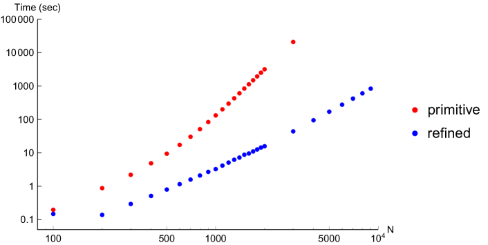
Figure 2: Timings (in seconds) for the primitive algorithm (upper curve) and refined algorithm (lower curve) applied to the numerical series (1.1).

	Primitive	Refined
$N$	algorithm	algorithm	Ratio
10	0.02	0.02	1.21
15	0.08	0.06	1.46
20	0.27	0.12	2.25
25	0.50	0.21	2.40
30	1.04	0.36	2.85
35	3.15	0.56	5.64
40	16.13	0.77	21.07
45	57.23	1.04	55.14
50	139.52	1.41	98.66
55	283.39	1.72	164.86
60	505.61	2.15	234.67
65	1029.79	2.90	355.29
70	5390.53	3.44	1567.81
75	20714.2	4.23	4893.62
80	54919.5	4.75	11560.1
90		6.35
100		8.60
110		10.79
120		13.52
130		16.54
140		19.97
150		24.06
160		28.42
170		33.76
180		39.46
190		45.91
200		52.23
300		158.25
400		360.65
500		691.27
600		1184.81
700		1910.57
800		2909.85
900		4244.91
1000		5960.16

Table 2: Timings (in seconds) for the primitive and refined algorithms applied to the polynomial series (1.2).

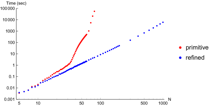
(a)

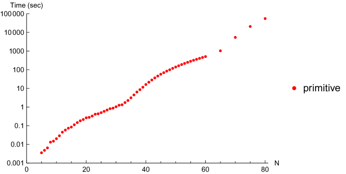
(b)

Figure 3: Timings (in seconds) for the primitive algorithm (upper curve) and refined algorithm (lower curve) applied to the polynomial series (1.2): log-log plot in (a), linear-log plot for the primitive algorithm in (b).

Some remarks. 1. When the primitive algorithm is programmed recursively in Mathematica, it is necessary to set $Recursion Limit to a large enough number (or Infinity) in order to avoid incomplete execution.

2. Because of quirks in Mathematica’s treatment of power series with symbolic coefficients, the primitive algorithm (in either version) applied to (1.2) becomes exceedingly slow for $N\mathrel{\hbox to0.0pt{\lower 3.0pt\hbox{$\mathchar 536\relax$}\hss}\raise 2.0pt\hbox{$\mathchar 318\relax$}}10$ if the basic step is programmed simply as f[k] = (1 - 1/f[k-1])/(alpha[k]*t). Instead, it is necessary to write f[k] = Map[Together, (1 - 1/f[k-1])/(alpha[k]*t)] in order to force the simplification of rational-function expressions to polynomials. I thank Daniel Lichtblau for this crucial suggestion. The results reported in Table 2 and Figure 3 refer to this latter version of the program.

3. The timings reported here were obtained using Mathematica’s command Timing, which under this operating system apparently includes the total CPU time in all threads. The real time elapsed was in some instances up to a factor $\approx 2$ smaller than this, due to partially parallel execution on this multi-core CPU.

4. One might wonder: Why on earth would one want to compute 1000 or more continued-fraction coefficients? One answer (perhaps not the only one) is that the nonnegativity of the S-fraction coefficients $\alpha_{n}$ is a necessary and sufficient condition for a sequence ${\bm{a}}=(a_{n})_{n\geq 0}$ of real numbers to be a Stieltjes moment sequence, i.e. the moments of a positive measure on $[0,\infty)$; this was shown by Stieltjes [96] in 1894. On the other hand, it is easy to concoct sequences that are not Stieltjes moment sequences but which have $\alpha_{n}>0$ until very high order. Consider, for instance, the sequence

$$a_{n}\;\stackrel{{\scriptstyle\rm def}}{{=}}\;(1+\epsilon)\,n!\,-\,{\epsilon\over(n+1)^{2}}\;=\;\int\limits_{0}^{\infty}x^{n}\>\Bigl{[}(1+\epsilon)e^{-x}\,+\,\epsilon\log x\Bigr{]}\>dx\;,$$ (10.1)

which fails to be a Stieltjes moment sequence whenever $\epsilon>0$ because the density is negative near $x=0$ (apply [92, Corollary 2.10]). For $\epsilon=1$, the first negative coefficient $\alpha_{n}$ is $n=6$; for $\epsilon=1/2$ it is $n=20$; for $\epsilon=1/4$ it is $n=178$; for $\epsilon=1/8$ it is some unknown (to me) $n>1500$. So it can be important to compute S-fraction coefficients to very high order when trying to determine empirically whether a given sequence is or is not a Stieltjes moment sequence. $\blacksquare$

11 Final remarks

The algorithm presented here is intended, in the first instance, for use in exact arithmetic: the field $F$ could be (for example) the field ${\mathbb{Q}}$ of rational numbers, or more generally the field ${\mathbb{Q}}(x_{1},\ldots,x_{n})$ of rational fractions in indeterminates $x_{1},\ldots,x_{n}$ with coefficients in ${\mathbb{Q}}$. I leave it to others to analyze the numerical (in)stability of this algorithm when carried out in $F={\mathbb{R}}$ or ${\mathbb{C}}$ with finite-precision arithmetic, and/or to devise alternative algorithms with improved numerical stability.

The continued fractions discussed here are what could be called classical continued fractions. Very recently combinatorialists have developed a theory of branched continued fractions, based on generalizing Flajolet’s master theorem (Theorem 8.1) to other classes of lattice paths. This idea was suggested by Viennot [101, section V.6], carried forward in the Ph.D. theses of Roblet [86] and Varvak [100], and then comprehensively developed by Pétréolle, Sokal and Zhu [83, 82]. There is a corresponding generalization of the Euler–Gauss recurrence method: for instance, for the $m$-S-fractions, which generalize the regular C-fractions, the recurrence (9.9) is generalized to

$$g_{k}(t)-g_{k-1}(t)\;=\;\alpha_{k+m}t\,g_{k+m}(t)\qquad\hbox{for }k\geq 0$$ (11.1)

for a fixed integer $m\geq 1$. Furthermore, Gauss’ [51] continued fraction for the ratio of contiguous hypergeometric functions ${{\tensor[_{2\!}]{F}{{}_{1}}\!}}$ can be generalized to ${\tensor[_{r\!}]{F}{{}_{s}}\!}$ for arbitrary $r,s$, where now $m=\max(r-1,s)$; the proof is based on (11.1). See [83] for details on all of this, and [82] for further applications. On the other hand, branched continued fractions are highly nonunique, and I do not know any algorithm for computing them.

Appendix

Answer to the exercise posed in Section 4:

$$g_{2j-1}(t)&=\sum_{n=0}^{\infty}\sum_{k=0}^{n}\genfrac{\{}{\}}{0.0pt}{}{n+j}{k+j}\,\binom{k+j-1}{k}\,x^{k}y^{n-k}\,t^{n}\\ g_{2j}(t)=\sum_{n=0}^{\infty}\sum_{k=0}^{n}\genfrac{\{}{\}}{0.0pt}{}{n+j}{k+j}\,\binom{k+j}{k}\,x^{k}y^{n-k}\,t^{n}$$ (A.1)

References

- [1] M. Aigner, Catalan and other numbers: a recurrent theme, in: Algebraic Combinatorics and Computer Science, edited by H. Crapo and D. Senato (Springer-Verlag Italia, Milan, 2001), pp. 347–390.
- [2] G.E. Andrews, The Theory of Partitions (Addison-Wesley, Reading MA, 1976). Reprinted with a new preface by Cambridge University Press, Cambridge, 1998.
- [3] G.E. Andrews, Euler’s pentagonal number theorem, Math. Mag. 56, 279–284 (1983).
- [4] G.E. Andrews, On the proofs of the Rogers–Ramanujan identities, in -Series and Partitions, IMA Volumes in Mathematics and its Applications #18, edited by D. Stanton (Springer, New York, 1989), pp. 1–14.
- [5] G.E. Andrews, Ramanujan’s “lost” notebook. VIII. The entire Rogers–Ramanujan function, Adv. Math. 191, 393–407 (2005).
- [6] G.E. Andrews, Ramanujan’s “lost” notebook. IX. The partial theta function as an entire function, Adv. Math. 191, 408–422 (2005).
- [7] G.E. Andrews and B.C. Berndt, Ramanujan’s Lost Notebook, Part I (Springer-Verlag, New York, 2005).
- [8] G.E. Andrews and B.C. Berndt, Ramanujan’s Lost Notebook, Part II (Springer-Verlag, New York, 2009).
- [9] R. Askey, Ramanujan and hypergeometric and basic hypergeometric series, in Ramanujan International Symposium on Analysis (Pune, 1987), edited by N.K. Thakare, K.C. Sharma and T.T. Raghunathan (Macmillan India, New Delhi, 1989), pp. 1–83; reprinted in Russian Math. Surveys 45(1), 37–86 (1990), and in Ramanujan: Essays and Surveys, edited by B.C. Berndt and R.A. Rankin (American Mathematical Society, Providence, RI, 2001), pp. 277–324.
- [10] M.F. Atiyah, Resolution of singularities and division of distributions, Comm. Pure Appl. Math. 23, 145–150 (1970).
- [11] G.A. Baker, Jr. and P. Graves-Morris, Padé Approximants, 2nd ed., Encyclopedia of Mathematics and its Applications #59 (Cambridge University Press, Cambridge, 1996).
- [12] E.J. Barbeau, Euler subdues a very obstreperous series, Amer. Math. Monthly 86, 356–372 (1979).
- [13] E.J. Barbeau and P.J. Leah, Euler’s 1760 paper on divergent series, Historia Math. 3, 141–160 (1976); errata and additions 5, 332 (1978).
- [14] B.C. Berndt, Ramanujan’s Notebooks, Part III (Springer-Verlag, New York, 1991).
- [15] I.N. Bernšteĭn, The analytic continuation of generalized functions with respect to a parameter, Funkcional. Anal. i Priložen. 6(4), 26–40 (1972) [= Funct. Anal. Appl. 6, 273–285 (1972)].
- [16] I.N. Bernšteĭn and S.I. Gel’fand, Meromorphy of the function , Funkcional. Anal. i Priložen. 3(1), 84–85 (1969) [= Funct. Anal. Appl. 3, 68–69 (1969)].
- [17] G. Bhatnagar, How to prove Ramanujan’s -continued fractions, in Ramanujan 125, Contemporary Mathematics #627, edited by K. Alladi, F. Garvan and A.J. Yee (American Math. Soc., Providence RI, 2014), pp. 49–68.
- [18] G. Bhatnagar, How to discover the Rogers–Ramunujan identities, Resonance 20(5), 416–430 (2015).
- [19] G. Bhatnagar, Ramanujan’s -continued fractions, preprint (August 2022), arXiv:2208.12656 [math.CA] at arXiv.org.
- [20] J.-E. Björk, Rings of Differential Operators (North-Holland, Amsterdam–Oxford–New York, 1979).
- [21] N. Bourbaki, Algebra II (Springer-Verlag, Berlin–Heidelberg–New York, 1990).
- [22] C. Brezinski, History of Continued Fractions and Padé Approximants, Springer Series in Computational Mathematics #12 (Springer-Verlag, Berlin, 1991).
- [23] T.S. Chihara, An Introduction to Orthogonal Polynomials (Gordon and Breach, New York–London–Paris, 1978). Reprinted by Dover, Mineola NY, 2011.
- [24] E.v.F. Conrad, Some continued fraction expansions of Laplace transforms of elliptic functions, PhD thesis, Ohio State University, 2002. Available on-line at http://rave.ohiolink.edu/etdc/view?acc_num=osu1029248229
- [25] E.v.F. Conrad and P. Flajolet, The Fermat cubic, elliptic functions, continued fractions, and a combinatorial excursion, Séminaire Lotharingien de Combinatoire 54, article B54g (2006).
- [26] S.C. Coutinho, A Primer of Algebraic -Modules, London Mathematical Society Student Texts #33 (Cambridge University Press, Cambridge, 1995).
- [27] A. Cuyt, V.B. Petersen, B. Verdonk, H. Waadeland and W.B. Jones, Handbook of Continued Fractions for Special Functions (Springer-Verlag, New York, 2008).
- [28] A. Cuyt and L. Wuytack, Nonlinear Methods in Numerical Analysis, North-Holland Mathematics Studies #136 = Studies in Computational Mathematics #1 (North-Holland, Amsterdam, 1987).
- [29] E. Deutsch, L. Ferrari and S. Rinaldi, Production matrices, Adv. Appl. Math. 34, 101–122 (2005).
- [30] E. Deutsch, L. Ferrari and S. Rinaldi, Production matrices and Riordan arrays, Ann. Comb. 13, 65–85 (2009).
- [31] D. Dumont, Pics de cycle et dérivées partielles, Séminaire Lotharingien de Combinatoire 13, article B13a (1986).
- [32] D. Dumont, A continued fraction for Stirling numbers of the second kind, unpublished note (1989), cited in [111].
- [33] D. Dumont and G. Kreweras, Sur le développement d’une fraction continue liée à la série hypergéométrique et son interprétation en termes de records et anti-records dans les permutations, European J. Combin. 9, 27–32 (1988).
- [34] D. Dumont and A. Randrianarivony, Sur une extension des nombres de Genocchi, European J. Combin. 16, 147–151 (1995).
- [35] G. Eisenstein, Théorèmes sur les formes cubiques et solution d’une équation du quatrième degré à quatre indéterminées, J. Reine Angew. Math. 27, 75–79 (1844).
- [36] G. Eisenstein, Transformations remarquables de quelques séries, J. Reine Angew. Math. 27, 193–197 (1844).
- [37] A. Elvey Price, private communication (May 2017).
- [38] A. Elvey Price and A.D. Sokal, Phylogenetic trees, augmented perfect matchings, and a Thron-type continued fraction (T-fraction) for the Ward polynomials, Electron. J. Combin. 27(4), #P4.6 (2020).
- [39] G. Eneström, Die Schriften Eulers chronologisch nach den Jahren geordnet, in denen sie verfaßt worden sind, Jahresbericht der Deutschen Mathematiker-Vereinigung (Teubner, Leipzig, 1913). [English translation, with explanatory notes, available at http://eulerarchive.maa.org/index/enestrom.html]
- [40] L. Euler, De fractionibus continuis dissertatio, Commentarii Academiae Scientiarum Petropolitanae 9, 98–137 (1744); reprinted in Opera Omnia, ser. 1, vol. 14, pp. 187–216. [English translation in Math. Systems Theory 18, 295–328 (1985). Latin original and English and German translations available at http://eulerarchive.maa.org/pages/E071.html]
- [41] L. Euler, De seriebus divergentibus, Novi Commentarii Academiae Scientiarum Petropolitanae 5, 205–237 (1760); reprinted in Opera Omnia, ser. 1, vol. 14, pp. 585–617. [Latin original and English and German translations available at http://eulerarchive.maa.org/pages/E247.html]
- [42] L. Euler, De transformatione seriei divergentis in fractionem continuam, Nova Acta Academiae Scientarum Imperialis Petropolitanae 2, 36–45 (1788); reprinted in Opera Omnia, ser. 1, vol. 16, pp. 34–46. [Latin original and English and German translations available at http://eulerarchive.maa.org/pages/E616.html]
- [43] P. Flajolet, Combinatorial aspects of continued fractions, Discrete Math. 32, 125–161 (1980).
- [44] P. Flajolet and J. Françon, Elliptic functions, continued fractions and doubled permutations, European J. Combin. 10, 235–241 (1989).
- [45] A. Folsom, Modular forms and Eisenstein’s continued fractions, J. Number Theory 117, 279–291 (2006).
- [46] Free Software Foundation, The GNU Multiple Precision Arithmetic Library, https://gmplib.org/
- [47] G. Frobenius, Ueber Relationen zwischen den Näherungsbrüchen von Potenzreihe, Journal für die reine und angewandte Mathematik 90, 1–17 (1881).
- [48] G. Frobenius and L. Stickelberger, Ueber die Addition und Multiplication der elliptischen Functionen, Journal für die reine und angewandte Mathematik 88, 146–184 (1879).
- [49] M. Galuzzi, Lagrange’s essay “Recherches sur la manière de former des tables des planètes d’après les seules observations”, Rev. Histoire Math. 1, 201–233 (1995).
- [50] G. Gasper and M. Rahman, Basic Hypergeometric Series, 2nd ed. (Cambridge University Press, Cambridge–New York, 2004).
- [51] C.F. Gauss, Disquisitiones generales circa seriem infinitam , Commentationes Societatis Regiae Scientiarum Gottingensis Recentiores, Classis Mathematicae 2 (1813). [Reprinted in C.F. Gauss, Werke, vol. 3 (Cambridge University Press, Cambridge, 2011), pp. 123–162.] Available on-line at http://gdz.sub.uni-goettingen.de/dms/load/toc/?PPN=PPN235999628
- [52] I.M. Gel’fand and G.E. Shilov, Generalized Functions, vol. 1 (Academic Press, New York–London, 1964).
- [53] R.G. Gordon, Error bounds in equilibrium statistical mechanics, J. Math. Phys. 9, 655–663 (1968).
- [54] I.P. Goulden and D.M. Jackson, Combinatorial Enumeration (Wiley, New York, 1983). Reprinted by Dover, Mineola NY, 2004.
- [55] R.L. Graham, D.E. Knuth and O. Patashnik, Concrete Mathematics: A Foundation for Computer Science, 2nd ed. (Addison-Wesley, Reading, Mass., 1994).
- [56] N.S.S. Gu and H. Prodinger, On some continued fraction expansions of the Rogers–Ramanujan type, Ramanujan J. 26, 323–367 (2011).
- [57] E. Heine, Untersuchungen über die Reihe , J. reine angew. Math. 34, 285–328 (1847). Available on-line at http://www.digizeitschriften.de/main/dms/img/?PPN=GDZPPN002145758
- [58] P. Henrici, Applied and Computational Complex Analysis, vol. 1 (Wiley-Interscience, New York–London–Sydney, 1974).
- [59] P. Henrici, Applied and Computational Complex Analysis, vol. 2 (Wiley-Interscience, New York–London–Sydney, 1977).
- [60] M.E.H. Ismail and J. Zeng, Addition theorems via continued fractions, Trans. Amer. Math. Soc. 362, 957–983 (2010).
- [61] W.B. Jones and W.J. Thron, Continued Fractions: Analytic Theory and Applications (Addison-Wesley, Reading MA, 1980).
- [62] A. Kasraoui and J. Zeng, Distribution of crossings, nestings and alignments of two edges in matchings and partitions, Electron. J. Combin. 13, #R33 (2006).
- [63] C.K. Kausler, Expositio methodi series quascunque datas in fractiones continuas convertendi, Mémoires de l’Académie Impériale des Sciences de St. Pétersbourg 1, 156–174 (1803–1806).
- [64] C.F. Kausler, Die Lehre von den Continuirlichen Brüchen: nebst ihren vorzüglichsten Anwendungen auf Arithmetik und Algebra vollständig abgehandelt (Franz Christian Löflund, Stuttgart, 1803). Available on-line at https://opacplus.bsb-muenchen.de/title/BV001436293
- [65] A.N. Khovanskii, The Application of Continued Fractions and their Generalizations to Problems in Approximation Theory, translated from the Russian by P. Wynn (Noordhoff, Groningen, 1963).
- [66] S. Khrushchev, Orthogonal Polynomials and Continued Fractions: From Euler’s Point of View, Encyclopedia of Mathematics and its Applications #122 (Cambridge University Press, Cambridge, 2008).
- [67] D.E. Knuth, Two notes on notation, Amer. Math. Monthly 99, 403–422 (1992).
- [68] M. Laczkovich, On Lambert’s proof of the irrationality of , Amer. Math. Monthly 104, 439–443 (1997).
- [69] J.-L. Lagrange, Recherches sur la manière de former des tables des planètes d’après les seules observations, Mémoires de l’Académie Royale des Sciences de Paris 1772, 513–618; reprinted in Œuvres, vol. 6, pp. 507–627. Available on-line at http://gallica.bnf.fr/ark:/12148/bpt6k229225j/f509
- [70] J.H. Lambert, Mémoire sur quelques propriétés remarquables des quantités transcendentes circulaires et logarithmiques, Mémoires de l’Académie Royale des Sciences de Berlin 17, 265–322 (1768). Available on-line at http://www.kuttaka.org/~JHL/L1768b.html
- [71] A.M. Legendre, Éléments de Géometrie, avec des notes, 3 édition (Firmin Didot, Paris, 1800). Available on-line at https://www.google.co.uk/books/edition/El%C3%A9ments_de_g%C3%A9om%C3%A9trie_avec_des_notes/SqpXAAAAYAAJ See also 11 édition (Firmin Didot, Paris, 1817), available on-line at https://gallica.bnf.fr/ark:/12148/bpt6k29403p [English translation: Elements of Geometry and Trigonometry, with notes, translated by D. Brewster (Oliver & Boyd, Edinburgh, 1822). Available on-line at https://www.google.co.uk/books/edition/Elements_of_Geometry_and_Trigonometry/RYMAAAAAMAAJ]
- [72] W. Leighton and W.T. Scott, A general continued fraction expansion, Bull. Amer. Math. Soc. 45, 596–605 (1939).
- [73] L. Lorentzen and H. Waadeland, Continued Fractions with Applications (North-Holland, Amsterdam, 1992).
- [74] Mathematics Stack Exchange, Who was V. Viskovatov?, https://math.stackexchange.com/questions/390522/who-was-v-viskovatov
- [75] S.C. Milne, Infinite families of exact sums of squares formulas, Jacobi elliptic functions, continued fractions, and Schur functions, Ramanujan J. 6, 7–149 (2002).
- [76] J.A. Murphy and M.R. O’Donohoe, Some properties of continued fractions with applications in Markov processes, J. Inst. Math. Appl. 16, 57–71 (1975).
- [77] J.A. Murphy and M.R. O’Donohoe, A class of algorithms for obtaining rational approximants to functions which are defined by power series, Z. Angew. Math. Phys. 28, 1121–1131 (1977).
- [78] I. Niven, Formal power series, Amer. Math. Monthly 76, 871–889 (1969).
- [79] M.R. O’Donohoe, Applications of continued fractions in one and more variables, Ph.D. thesis, Brunel University (1974). Available on-line at http://bura.brunel.ac.uk/handle/2438/5800
- [80] P. Peart and W.-J. Woan, Generating functions via Hankel and Stieltjes matrices, J. Integer Seq. 3, article 00.2.1 (2000).
- [81] O. Perron, Die Lehre von den Kettenbrüchen (Teubner, Leipzig, 1913). Second edition: Teubner, Leipzig, 1929; reprinted by Chelsea, New York, 1950. Third edition, 2 vols.: Teubner, Stuttgart, 1954, 1957.
- [82] M. Pétréolle and A.D. Sokal, Lattice paths and branched continued fractions, II: Multivariate Lah polynomials and Lah symmetric functions, European J. Combin. 92, 103235 (2021).
- [83] M. Pétréolle, A.D. Sokal and B.-X. Zhu, Lattice paths and branched continued fractions: An infinite sequence of generalizations of the Stieltjes–Rogers and Thron–Rogers polynomials, with coefficientwise Hankel-total positivity, preprint (July 2018), arXiv:1807.03271 [math.CO] at arxiv.org, to appear in Memoirs of the American Mathematical Society.
- [84] K.G. Ramanathan, Hypergeometric series and continued fractions, Proc. Indian Acad. Sci. (Math. Sci.) 97, 277–296 (1987).
- [85] S. Ramanujan and L.J. Rogers, Proof of certain identities in combinatory analysis, Proc. Cambridge Philos. Soc. 19, 211–216 (1919).
- [86] E. Roblet, Une interprétation combinatoire des approximants de Padé, Thèse de doctorat, Université Bordeaux I (1994). Reprinted as Publications du Laboratoire de Combinatoire et d’Informatique Mathématique (LACIM) #17, Université du Québec à Montréal (1994). Available on-line at http://lacim.uqam.ca/en/les-parutions/
- [87] E. Roblet and X.G. Viennot, Théorie combinatoire des T-fractions et approximants de Padé en deux points, Discrete Math. 153, 271–288 (1996).
- [88] L.J. Rogers, Second memoir on the expansion of certain infinite products, Proc. London Math. Soc. 25, 318–343 (1894).
- [89] L.J. Rogers, On the representation of certain asymptotic series as convergent continued fractions, Proc. London Math. Soc. (series 2) 4, 72–89 (1907).
- [90] A.V. Sills, An Invitation to the Rogers–Ramanujan Identities (CRC Press, Boca Raton, 2018).
- [91] A.D. Sokal, The leading root of the partial theta function, Adv. Math. 229, 2603–2621 (2012).
- [92] A.D. Sokal, The Euler and Springer numbers as moment sequences, Expo. Math. 38, 1–26 (2020).
- [93] A.D. Sokal, Coefficientwise total positivity (via continued fractions) for some Hankel matrices of combinatorial polynomials, in preparation.
- [94] A.D. Sokal and J. Zeng, Some multivariate master polynomials for permutations, set partitions, and perfect matchings, and their continued fractions, Adv. Appl. Math. 138, 102341 (2022).
- [95] T.J. Stieltjes, Sur la réduction en fraction continue d’une série procédant selon les puissances descendantes d’une variable, Ann. Fac. Sci. Toulouse 3, H1–H17 (1889).
- [96] T.J. Stieltjes, Recherches sur les fractions continues, Ann. Fac. Sci. Toulouse 8, J1–J122 (1894) and 9, A1–A47 (1895). [Reprinted, together with an English translation, in T.J. Stieltjes, Œuvres Complètes/Collected Papers (Springer-Verlag, Berlin, 1993), vol. II, pp. 401–566 and 609–745.]
- [97] W.J. Thron, Some properties of continued fractions , Bull. Amer. Math. Soc. 54, 206–218 (1948).
- [98] J. Touchard, Nombres exponentiels et nombres de Bernoulli, Canad. J. Math. 8, 305–320 (1956).
- [99] V.S. Varadarajan, Euler and his work on infinite series, Bull. Amer. Math. Soc. 44, 515–539 (2007).
- [100] A.L. Varvak, Encoding properties of lattice paths, Ph.D. thesis, Brandeis University, May 2004. Available on-line at http://people.brandeis.edu/~gessel/homepage/students/varvakthesis.pdf
- [101] G. Viennot, Une théorie combinatoire des polynômes orthogonaux généraux, Notes de conférences données à l’Université du Québec à Montréal, septembre-octobre 1983. Available on-line at http://www.xavierviennot.org/xavier/polynomes_orthogonaux.html
- [102] B. Viscovatov, De la méthode générale pour réduire toutes sortes de quantités en fractions continues, Mémoires de l’Académie Impériale des Sciences de St. Pétersbourg 1, 226–247 (1803–1806).
- [103] H.S. Wall, Note on a certain continued fraction, Bull. Amer. Math. Soc. 51, 930–934 (1945).
- [104] H.S. Wall, Analytic Theory of Continued Fractions (Van Nostrand, New York, 1948).
- [105] R. Wallisser, On Lambert’s proof of the irrationality of , in Algebraic Number Theory and Diophantine Analysis, edited by F. Halter-Koch and R.F. Tichy (de Gruyter, Berlin, 2000), pp. 521–530.
- [106] G.N. Watson, Theorems stated by Ramanujan (VII): Theorems on continued fractions, J. London Math. Soc. 4, 39–48 (1929).
- [107] P.J.S. Watson, Algorithms for differentiation and integration, in Padé Approximants and their Applications, edited by P.R. Graves-Morris (Academic Press, London–New York, 1973), pp. 93–97.
- [108] Wikipedia, Gauss’s continued fraction, http://en.wikipedia.org/wiki/Gauss%27s_continued_fraction
- [109] H.S. Wilf, generatingfunctionology, 2nd ed. (Academic Press, San Diego–London, 1994).
- [110] W.-J. Woan, Hankel matrices and lattice paths, J. Integer Seq. 4, article 01.1.2 (2001).
- [111] J. Zeng, The -Stirling numbers, continued fractions and the -Charlier and -Laguerre polynomials, J. Comput. Appl. Math. 57, 413–424 (1995).
- [112] J. Zeng, Combinatorics of orthogonal polynomials and their moments, in Lectures on Orthogonal Polynomials and Special Functions, edited by H.S. Cohl and M.E.H. Ismail, London Mathematical Society Lecture Note Series #464 (Cambridge University Press, Cambridge, 2021), pp. 280–334.