Effect of Temperature Gradient on Quantum Transport
	Amartya Bose,∗a and Peter L. Waltersb,c

The recently introduced multisite tensor network path integral (MS-TNPI) method [Bose and Walters, J. Chem. Phys., 2022, 156, 24101.] for simulation of quantum dynamics of extended systems has been shown to be effective in studying one-dimensional systems. Quantum transport in these systems are typically studied at a constant temperature. However, temperature seems to be a very obvious parameter that can be spatially changed to control the quantum transport. Here, MS-TNPI is used to study “non-equilibrium” effects of an externally imposed temperature gradient on the quantum transport in one-dimensional extended quantum systems.

Quantum transport in extended open systems has been one of the holy-grails of quantum dynamics. It combines the difficulty of treating extended quantum systems with the difficulty of treating open quantum systems, both of which potentially lead to exponential growth of computational complexity. However, such systems are ubiquitous in nature, and hence of great importance. From magnetic materials to molecular aggregates, a vast variety of interesting physical phenomena lend themselves to be modeled as extended one-dimensional quantum systems interacting with an open thermal environment. Wave function-based methods such as density matrix renormalization group ^{1, 2, 3, 4, 5, 6} (DMRG) and multi-configuration time-dependent Hartree ^{7, 8, 9} (MCTDH and ML-MCTDH) and related methods have proven to be exceptionally useful in simulating the dynamics of extended quantum systems. However, due to their computational complexity, these methods are typically less useful when it comes to simulations pertaining to open quantum systems.

Path integrals have often been presented as a viable solution to the problem of calculating and storing of the wave functions for these open quantum systems. With these methods, the main challenge is that the number of paths considered in the path integral increases exponentially with the number of time steps. However, this exponential proliferation of the system path list can be curtailed through the use of an iterative procedure that exploits the rapid decay of correlation between well-separated time points. Although the computational complexity still increases exponentially with the number of time points retained within memory ($L$), this is usually much smaller then the number of points in the simulation. The quasi-adiabatic propagator path integral ^{10, 11, 12, 13} (QuAPI) methods, which are based on Feynman-Vernon influence functional, ¹⁴ make simulations of general open quantum systems much more approachable. Of late, the usage of tensor networks to facilitate simulations with influence functionals has also become quite common.^{15, 16, 17, 18} Ideas from these tensor network-based influence functional methods have motivated a recent extension of DMRG to simulating the dynamics of extended open quantum systems.¹⁹ This multisite tensor network path integral (MS-TNPI) method has also been used to explore the dynamics and spectrum of the B850 ring of the light harvesting subsystem²⁰ and study the effects of phononic scattering on quantum transport.²¹

Path integrals for extended open quantum systems suffer from a huge problem of exponential scaling. First, the presence of the thermal environment leads to an exponential scaling with respect to the number of time steps within memory. The base of this exponential scaling is related to the dimensionality of the system. For extended systems, the dimensionality is the product of the dimensions of the individual “sites” or “entities.” So, for a system with say 16 two-level systems, like the one used to model the B850 ring in Ref. ²⁰, the base of the scaling is $2^{16}$. So, if the memory length is $L$, the computational complexity is effectively $2^{16\times 2\times L}$. This is the problem that MS-TNPI solves by using a DMRG-like decomposition of the system along the various sites along with a decomposition of the “paths” along the temporal dimension.

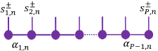
Fig.  1: Schematic of a density matrix of an extended system represented as an MPS.

DMRG and DMRG-like methods proceed by decomposing the system along the spatial dimension. By exploiting the lack of correlation between distant sites, the resulting matrix product state (MPS) can be an extremely compact and efficient representation of the system. The reduced density matrix after the $n$^th time step can expressed in the form of an MPS as follows

$$\tilde{\rho}(S^{\pm}_{n},n\Delta t) =\sum_{\left\{\alpha_{(j,n)}\right\}}A_{\alpha_{(1,n)}}^{s^{\pm}_{1,n}}A_{\alpha_{(1,n)},\alpha_{(2,n)}}^{s^{\pm}_{2,n}}\cdots A_{\alpha_{(P-1,n)}}^{s^{\pm}_{P,n}},$$ (1)

where $\alpha_{j,n}$ is the index connecting the $j$^th site at time-step $n$ to the $(j+1)$^th site at the same time step. Figure 1 gives a graphical representation of this structure. In the notation used here, the forward-backward state of the $j$^th site at the $n$^th time point is denoted by $s^{\pm}_{j,n}$ and the states of all the sites at this time step are collectively represented by $S_{n}^{\pm}$. (Here, the forward-backward state is a combination of the forward, bra, and backward, ket, states of the density matrix.) When the density matrix is represented as an MPS, the forward-backward propagator, which evolves it in time, must be represented as a matrix product operator (MPO).

With this setup, it is possible to obtain the time-dynamics of the isolated system through a series of MPO-MPS applications. However, often the individual sites interact with separate dissipative environments:

$$\hat{H} =\hat{H}_{0}+\sum_{j=1}^{P}\sum_{l=1}^{N_{\text{osc}}}\frac{p_{jl}^{2}}{2m_{jl}}+\frac{1}{2}m_{jl}\omega_{jl}^{2}\left(x_{jl}-\frac{c_{jl}\hat{s}_{j}}{m_{jl}\omega_{jl}^{2}}\right)^{2}$$ (2)

where $\hat{H}_{0}$ is the Hamiltonian corresponding to the isolated extended system with $P$ units or particles. Each unit or particle is coupled to a dissipative environment, which under Gaussian response theory can be mapped on to a set of $N_{\text{osc}}$ harmonic oscillators. The $l$^th harmonic oscillator of the $j$^th system unit interacts with it through the operator $\hat{s}_{j}$ with a strength of $c_{jl}$. The frequencies and couplings of the baths are often given in terms of the spectral density, which can be related to the Fourier transform of the energy gap autocorrelation function.

In the the presence of the dissipative environment, the time evolution of the reduced density matrix can be described as

$$\tilde{\rho}(S^{\pm}_{N},N\Delta t) =\sum_{S_{0}^{\pm}}\sum_{S^{\pm}_{1}}\cdots\sum_{S^{\pm}_{N-1}}\tilde{\rho}(S^{\pm}_{0},0)P_{S_{0}^{\pm}\cdots S^{\pm}_{N}}$$ (3)

$$=\sum_{S_{0}^{\pm}}\sum_{S^{\pm}_{1}}\cdots\sum_{S^{\pm}_{N-1}}\tilde{\rho}(S^{\pm}_{0},0)P^{(0)}_{S_{0}^{\pm}\cdots S^{\pm}_{N}}F\left[\left\{S^{\pm}_{n}\right\}\right].$$ (4)

Here, $P^{(0)}_{S_{0}^{\pm}\cdots S^{\pm}_{N}}$ is the bare path amplitude tensor, which contains the full information of the isolated system, and $F$ is the Feynman-Vernon influence functional ¹⁴, which depends entirely on the spectral density and encodes the system-environment interaction. Lastly, $P_{S_{0}^{\pm}\cdots S^{\pm}_{N}}$ is the path amplitude tensor, which describes the system in the presence of the solvent. Since the dimensionality of the path amplitude tensor grows exponentially with the number of particles and time steps, it can only be explicitly constructed in a very small number of cases.

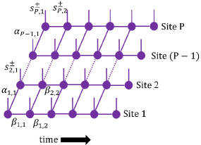
Fig.  2: Schematic of the two-dimensional MS-TNPI tensor network.

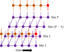
Fig.  3: Schematic of incorporation of influence functional in the MS-TNPI tensor network shown only for the first and last sites.

MS-TNPI ¹⁹ avoids this exponential scaling by performing a spatial decomposition of the bare system and combining it with a temporal decomposition of the influence functional to produce a compact two-dimensional tensor network representation of the path amplitude tensor,

$$P_{S_{0}^{\pm}\cdots S_{N}^{\pm}} =\sum_{\left\{\beta_{n}\right\}}\mathbb{T}^{S_{0}^{\pm}}_{\beta_{0}}\cdots\mathbb{T}^{S_{n}^{\pm}}_{\beta_{n-1},\beta_{n}}\cdots\mathbb{T}_{\beta_{N-1}}^{S_{N}^{\pm}}.$$ (5)

Here, $\beta_{n}$ is the index connecting the tensors at time-point $n$ to the ones at $n+1$, and each $\mathbb{T}$ is a matrix product representation decomposed along the site axis. The resulting two-dimensional tensor network is shown in Fig. 2. Each of the columns roughly contains the state of the full system at any point of time. Therefore, when contracting the network along the columns, we get the full reduced density matrix corresponding to the extended system. Naïvely speaking, the number of columns in the MS-TNPI network corresponds to the total length of the simulation. However, an iterative procedure can be employed that effectively reduces the number columns to the length of the memory induced by the baths. The rows represent the path amplitude corresponding to the individual sites or units of the system. This allows both the incorporation of the Feynman-Vernon influence functional in a transparent manner as MPOs acting on the rows as shown in Fig. 3 and the truncation of memory.

The present paper uses MS-TNPI to explore the effects of temperature differences on quantum transport in extended open systems. Such temperature differences can be caused by an external temperature gradient being applied across a molecular wire or more commonly as a side-effect of heat generated during excitation caused by lasers. Irrespective of the origin of such temperature differences, it provides us with a potentially useful parameter for controlling and changing the characteristics of the quantum transport. This is a first step in exploring such changes brought onto the population dynamics caused by such temperature gradients. In this work, we focus exclusively on the Frenkel exciton transfer model. The system Hamiltonian is given by

$$\hat{H}_{0} =\epsilon\sum_{j=1}^{P}\outerproduct{e_{j}}{e_{j}}+\hbar J\sum_{j=1}^{P}\left(\outerproduct{e_{j}}{e_{j+1}}+\outerproduct{e_{j}}{e_{j+1}}\right)$$ (6)

where $J$ is the excitonic coupling between the different sites, $\epsilon$ is the excitation energy of the sites and lastly, $\ket{e_{j}}$ is the many-body wavefunction with just the $j$^th site excited. In terms of the one-body ground, $\ket{\phi^{g}_{j}}$, and excited, $\ket{\phi^{e}_{j}}$, wavefunctions, $\ket{e_{j}}=\ket{\phi^{e}_{j}}\otimes\prod_{k\neq j}\ket{\phi^{g}_{k}}$. The system-bath interaction takes place through $\hat{s}_{j}$, which defined as $\hat{s}_{j}\ket{\phi^{e}_{j}}=\ket{\phi^{e}_{j}}$ and $\hat{s}_{j}\ket{\phi^{g}_{j}}=0$.

As our first example, we consider a 31 site system with $\hbar J=1$ and $\epsilon=100$. (The sites are numbered from 1 to 31.) The vibrational bath is site independent and characterized by the following spectral density:

$$J(\omega) =\frac{\pi}{2}\hbar\xi\omega\exp\left(-\frac{\omega}{\omega_{c}}\right)$$ (7)

where $\omega_{c}=8J$ is the cutoff frequency and the dimensional Kondo parameter, $\xi=0.075$. We will study the dynamics of the system under an average temperature of $k_{B}\bar{T}=\hbar J$ and a temperature gradient of 0 and $0.05\hbar J/k_{B}$ per site. The temperature is lowest at the bottom end where the units have lower numbers and rises as we move up. The system with a zero temperature gradient is going to be used as a reference for comparisons. The excited state population dynamics, $P^{\text{exc}}_{j}(t)=\matrixelement{\phi^{e}_{j}}{\tilde{\rho}(t)}{\phi^{e}_{j}}$, corresponding to an initial state of $\tilde{\rho}(0)=\outerproduct{e_{16}}{e_{16}}$, in the absence of any temperature gradient is presented in Fig. 4. Because the middle unit is initially excited, the dynamics is completely symmetric, that is the populations of the units equidistant from the edges are identical. To explore this symmetry of dynamics, a site-symmetrized excited state population and a deviation measure are defined as follows:

$$\bar{P}^{\text{exc}}_{j}(t) =\frac{P^{\text{exc}}_{j}(t)+P^{\text{exc}}_{P-j+1}(t)}{2}$$ (8)

$$\delta{P}^{\text{exc}}_{j}(t) =\frac{P^{\text{exc}}_{j}(t)-\bar{P}^{\text{exc}}_{j}(t)}{\bar{P}^{\text{exc}}_{j}(t)}\times 100.$$ (9)

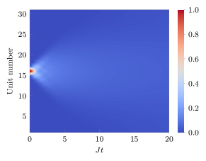
Fig.  4: Unit dependent excited state population, $P^{\text{exc}}_{j}(t)$, when no temperature gradient is applied.

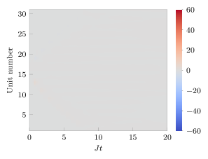
(a) $\delta{P}^{\text{exc}}_{j}(t)$ in absence of any temperature gradient.

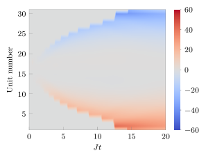
(b) $\delta{P}^{\text{exc}}_{j}(t)$ in presence of a temperature gradient of $0.05\hbar J/k_{B}$ per site.

Fig.  5: Plots of $\delta{P}^{\text{exc}}_{j}(t)$ in presence and absence of a temperature gradient for Frenkel model coupled to Ohmic bath.

This is demonstrated in Fig. 5 (a). The imposition of an external temperature gradient breaks this symmetry, leading to deviations in the excited state population dynamics as shown in Fig. 5 (b). For the linear ramp considered, the transport process seems to preferentially move the exciton to the colder monomers. The deviations are quite significant with an upper limit of around $\pm 50\%$.

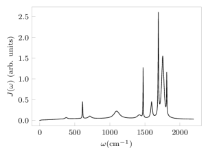
Fig.  6: Spectral density describing the molecular vibrations and the impact of the proteins on the dynamics of the B850 ring from Ref. ²²

As a more realistic example of exciton transfer, consider a chain of 31 bacteriochlorophyll (BChl) units. The intermonomer electronic coupling is taken to be $156.5\text{\,}{\mathrm{cm}}^{-1}$ and the excitation energy of a BChl unit is taken to be $12\,390\text{\,}{\mathrm{cm}}^{-1}$. The local spectral density was calculated using the molecular dynamics-based (MD) bath response function, $C_{\text{MD}}(t)$, reported in Ref. ²² using the following relation:

$$J(\omega) =\frac{\hbar\omega\beta_{\text{MD}}}{2}\int_{0}^{\infty}C_{\text{MD}}(t)\cos(\omega t)\differential{t}.$$ (10)

The resultant spectral density is shown in Fig. 6. Note that the inverse temperature used here, $\beta_{\text{MD}}$, corresponds to MD simulation setup. The spectral density, Eq. 10, is independent of the temperature of the path integral simulations done here. So, just as in the previous example, all the monomer units have identical spectral densities here as well. The dynamics and absorption spectrum of the B850 ring with this MD-based solvent has already been studied using MS-TNPI. ²⁰ We want to understand the changes brought about in the dynamics through an external temperature gradient of $10\text{\,}\mathrm{K}\mathrm{/}\text{unit}$. The average temperature of the chain is held at $300\text{\,}\mathrm{K}$.

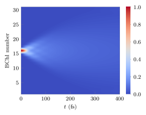
Fig.  7: Excitonic population dynamics in a BChl chain in absence of temperature gradient.

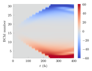
Fig.  8: Difference between excitonic population dynamics for a system with temperature gradient and the same system without a temperature gradient.

To study the effect of an external temperature gradient on this system, let us focus once again on exciting the middle bacteriochlorophyll unit (unit 16). In absence of any external temperature gradient, the populations of the sites is symmetric at all times. This dynamics is shown in Fig. 7. Figure 8 shows the difference caused in the excitonic population dynamics by the externally imposed temperature gradient. Note that despite having a structured spectral density, the trends here are identical to the model example, Fig. 5. Even in this case, population preferentially moves towards the colder end of the chain.

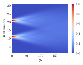
Fig.  9: Excitonic population dynamics in a BChl chain starting from a state with two excitons on the 6^th and the 10^th monomers.

Consider next the possibility of multiple excitons in the system. Suppose we start from the initial state $\tilde{\rho}=\outerproduct{e_{11}e_{21}}{e_{11}e_{21}}$. So, the 11^th and the 21^th monomers are in the excited states and everything else is in the ground state. The dynamics of this system in absence of any temperature gradient is shown in Fig. 9. On imposing the same external temperature gradient, the transport of both the excitons get affected. The excitonic population difference from the transport in absence of the temperature gradient is shown in Fig. 10. This time, we predictably see a superposition of the same pattern as the single excitation case for each of the two centers of excitation. The region between the two initial excitations, that is monomers 11 and 21 show this interplay.

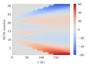
Fig.  10: Difference between the excitonic population dynamics in a BChl chain starting from a state with two excitons on the 6^th and the 10^th monomers in presenece and absence of temperature gradient.

We have demonstrated a noticeable change in the quantum transport of excitons in the presence of a temperature gradient. The excitonic population seems to travel preferentially to the colder end of the chain. This trend is consistent between model spectral densities and structured ones derived from molecular dynamics simulations. Investigations on the effect of temperature on the spectra and other properties will also be undertaken in the future. What has been shown in this communication seems to indicate that temperature might be a useable control for quantum dynamics. Different temperature profiles may affect the dynamics in interesting ways, opening up possibilities of using it to promote desired outcomes, like an increased quantum yield on a site, in the dynamics. Further exploration of these aspects would be done in the future.

Author Contributions

Both authors contributed equally to the design, implementation and writing of this paper.

Conflicts of interest

There are no conflicts to declare.