Line-Intensity Mapping: Theory Review

Abstract

Line-intensity mapping (LIM) is an emerging approach to survey the Universe, using relatively low-aperture instruments to scan large portions of the sky and collect the total spectral-line emission from galaxies and the intergalactic medium. Mapping the intensity fluctuations of an array of lines offers a unique opportunity to probe redshifts well beyond the reach of other cosmological observations, access regimes that cannot be explored otherwise, and exploit the enormous potential of cross-correlations with other measurements. This promises to deepen our understanding of various questions related to galaxy formation and evolution, cosmology, and fundamental physics.

Here we focus on lines ranging from microwave to optical frequencies, the emission of which is related to star formation in galaxies across cosmic history. Over the next decade, LIM will transition from a pathfinder era of first detections to an early-science era where data from more than a dozen missions will be harvested to yield new insights and discoveries. This review discusses the primary target lines for these missions, describes the different approaches to modeling their intensities and fluctuations, surveys the scientific prospects of their measurement, presents the formalism behind the statistical methods to analyze the data, and motivates the opportunities for synergy with other observables. Our goal is to provide a pedagogical introduction to the field for non-experts, as well as to serve as a comprehensive reference for specialists.

1 Introduction

In the past couple of decades, cosmology has become a precision science, with increasingly detailed measurements of the cosmic microwave background (CMB) and ever-larger surveys of galaxies yielding percent-level constraints on the parameters of the standard model of cosmology, $\Lambda$CDM, and informing sophisticated models of galaxy formation and evolution. In spite of this success, the nature of key theoretical pillars of $\Lambda$CDM remains elusive, the evolution of galaxy properties is largely unconstrained and several experimental tensions that have arisen warrant explanation. Looking forward, novel cosmological observables will be crucial to making progress in this quest to deepen our understanding of the cosmos.

Line-intensity mapping (LIM) 1979MNRAS.188..791H ; Suginohara:1998ti ; Chang:2007xk ; Visbal:2010rz ; Visbal:2011ee ; Gong:2011ts ; Carilli:2011vw ; Fonseca:2016qqw ; Kovetz:2017agg measures the integrated emission of spectral lines originating from many individually unresolved galaxies and the diffuse intergalactic medium (IGM). It tracks the makeup and growth of cosmic structure as well as the history of the astrophysical processes controlling galaxy formation and evolution. Unlike galaxy surveys, LIM does not require resolved high-significance detections but uses all incoming photons from any source within the field of view, obtaining tomographic line-of-sight information from targeting a known spectral line at different frequencies. This enables the use of smaller low-aperture instruments with modest experimental budgets to rapidly survey large areas of sky for studying cosmology and large-scale astrophysics. Through its intrinsic dependence on cosmology and astrophysics, LIM connects the smallest and largest scales in the Universe as no other observable can do.

There has been a flurry of interest in LIM in recent years with an impressive lineup of experimental projects pursuing an array of atomic and molecular spectral lines across the electromagnetic spectrum, from the radio to the ultraviolet. Simultaneously, the theoretical framework of the modeling of line intensities and the study of the line-intensity maps have vastly developed.

The focus of this review will be on spectral lines associated with gas cooling and star formation in galaxies, ranging from the rotational carbon-monoxide (CO) transitions observed in the sub-mm, through bright fine-structure lines such as [CII] in the far-infrared, to the hydrogen H$\alpha$ and Ly$\alpha$ lines in the optical and ultraviolet. The HI 21-cm line originating from the neutral hydrogen permeating the intergalactic medium in the early-Universe and from pockets within galaxies post-reionization has been reviewed in Refs. Furlanetto:2006jb ; Morales:2009gs ; Pritchard:2011xb ; Liu:2019awk .

As this review will advocate, LIM holds promise to become a cornerstone for our future understanding of cosmology and astrophysics, as the CMB and galaxy surveys have been so far. With just a handful of preliminary detections to date, this declaration may seem premature, but several properties such as its unprecedented reach, unique access, and extended overlap, suggest that LIM offers unique advantages in mapping the large-scale structure in the Universe.

Circumventing the requirement of individual source detection, LIM avoids the intrinsic depth limitation of surveys of galaxies, which are increasingly faint and sparse at high redshift. There are proposals to extend galaxy surveys to high redshifts (e.g. Ref. Schlegel:2019eqc ), but in such regimes LIM may yield more efficient mapping of cosmological perturbations Uzgil:2014pga ; Cheng:2018hox ; Schaan:2021hhy , with markedly lower budgets.

Figure 1 demonstrates the power of LIM in terms of reach. In a simulated volume spanning 1 deg² on the sky and a redshift slice $z=[4.9,5.1]$, we compare the total distribution of galaxies with those that could be realistically observed by a galaxy survey, and show the corresponding emission that would be detected by LIM experiments targeting CO(1-0) and [CII], respectively (not including instrumental noise nor contaminants, to ease the comparison). We see that each LIM experiment, with its own resolution limits, has the potential to detect fluctuations even where the galaxy survey would observe a void, with independent line emissions exhibiting different fluctuation amplitudes. While this example helps uncover the potential of LIM to augment and reach beyond existing techniques, it merely brushes the tip of the iceberg.

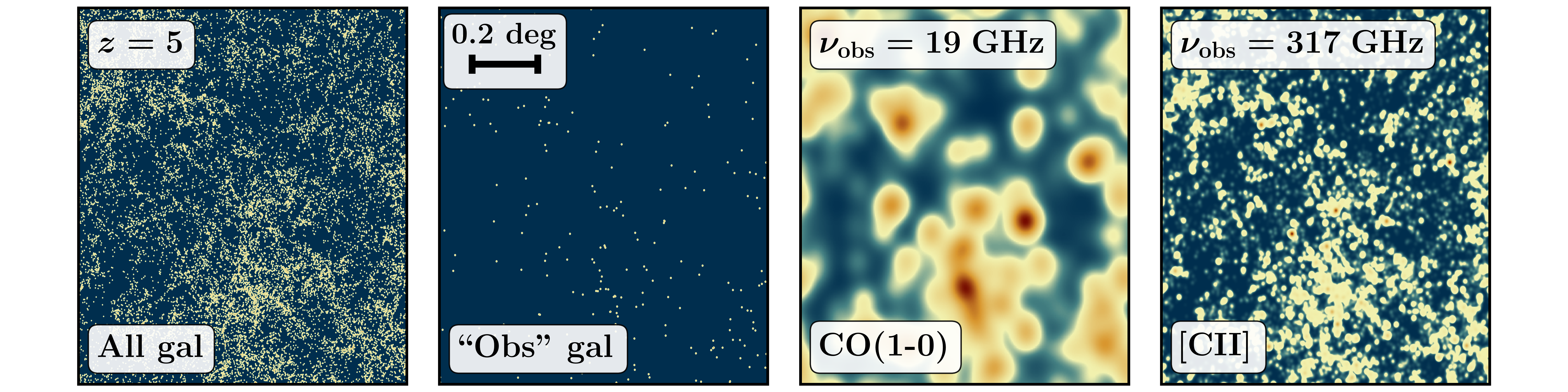
Figure 1: A 1 deg² field at $z\in\left[4.9,5.1\right]$ showing (from left to right) all the galaxies, “observable” galaxies (assuming an arbitrary cut off in the stellar masses $\geq 10^{9.5}\,M_{\odot}$ as a theoretical proxy for detection threshold), and maps of the CO and [CII] intensity fluctuations from this field. Characteristic angular resolutions of instruments targeting each line (4’ and 0.5’ for CO and CII, respectively) are applied. Results obtained using the approach of Ref. LC_paper , assuming parameterizations from Ref. 2016ApJ…829…93K and Ref. DeLooze:2014dta .

In terms of access, LIM is uniquely poised to probe crucial epochs in the history of our Universe, as illustrated in Fig. 2. Collecting all incoming photons, LIM directly probes the epoch of reionization (EoR), the IGM, the interstellar medium (ISM) and the formation and makeup of stars, granting access to astrophysical and cosmological information inaccessible otherwise since it is sensitive to the whole population of emitters instead of only the brightest ones. This also makes LIM more robust against selection effects and misestimation of line-emission and luminosity ratios whenever one line has extended emission.

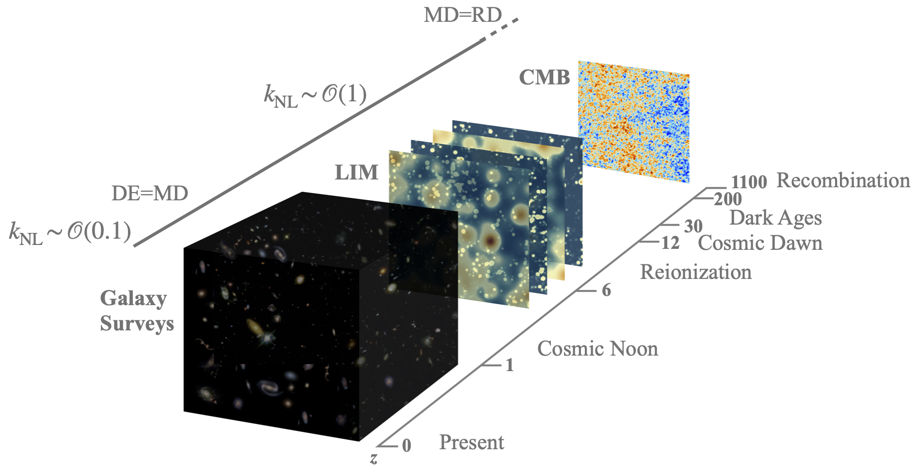
Figure 2: Intensity mapping of multiple line emissions provides rich access to redshift volumes otherwise inaccessible, enabling detailed study of various important epochs in cosmic history. Above the arrow of time on the left, MD=RD and DE=MD denote the redshifts of matter-radiation, and dark energy-matter equality, respectively, and $k_{\rm NL}$ is a rough estimation of the scale at which matter clustering becomes non linear, specified in units of ${\rm Mpc}^{-1}$.

Furthermore, extending the reach of a survey to higher redshifts increases the volume observed dramatically. This allows us to probe larger scales, potentially reaching scales of the order of the horizon, where signatures of inflation may be present. Moreover, as redshift grows, non-linear matter clustering is confined to ever-smaller scales, facilitating the theoretical interpretation. Although the access to small scales depends on the experimental resolution and the growing contribution of non-linear bias terms may hinder the ability to extract robust information from them Desjacques:2016bnm ; MoradinezhadDizgah:2021dei , exploring small scales will significantly increase the constraining power of LIM surveys. Considering different science targets introduces a tradeoff between deeper and wider surveys.

In terms of overlap, there is tremendous potential for LIM cross correlations. First, multi-line analyses allow for a multi-phase and multi-scale study of galaxy properties 2019ARA&A..57..511K , but also for a statistically more powerful study of large-scale structure to probe deviations from $\Lambda$CDM. Line-intensity maps can also be cross-correlated with galaxy surveys, with CMB observations—to study CMB secondary anisotropies such as weak gravitational lensing and the Sunyaev-Zel’dovich effect—and with catalogs of astrophysical transients such as gravitational waves from merging black holes and fast radio bursts.

The vast range of targeted wavelengths necessitates the use of different LIM instruments. Hence, instrumental and observational challenges and sources of contamination are not shared by all experiments, which renders the joint scope of LIM observations cleaner. Over the coming decade, more than a dozen ground-based, balloon-borne and space satellite experiments are expected to deliver line-intensity maps spanning the full history of the Universe from the present day to the EoR. As shown in Fig. 3, LIM surveys will gradually cover larger sky areas, as the field transitions from the current pathfinder era of first detections, to an early science era where they can be used to augment other measurements—particularly exploiting cross-correlation opportunities with other observables—and make advances in a plethora of areas in astrophysics and cosmology. Representatives of these eras include ongoing and funded experiments such as: COPSS Keating:2015qva ; Keating:2016pka , mmIME Keating:2020wlx , COMAP Cleary:2021dsp ; COMAP:2021nrp , FYST CCAT-Prime:2021lly and SPT-SLIM Karkare:2021ryi , targeting CO; CONCERTO 2020A&A…642A..60C , TIME 2014SPIE.9153E..1WC ; Sun:2020mco , FYST and the balloon-borne EXCLAIM 2021JATIS…7d4004S and TIM 2020arXiv200914340V , targeting [CII]; HETDEX Hill:2008mv ; Gebhardt:2021vfo , which will map Ly$\alpha$; and the SPHEREx satellite 2014arXiv1412.4872D , which will measure [OII], [OIII], H$\alpha$ and Ly$\alpha$. Figure 3 also shows the smallest scales accessible by this group of experiments, including their redshift dependence.

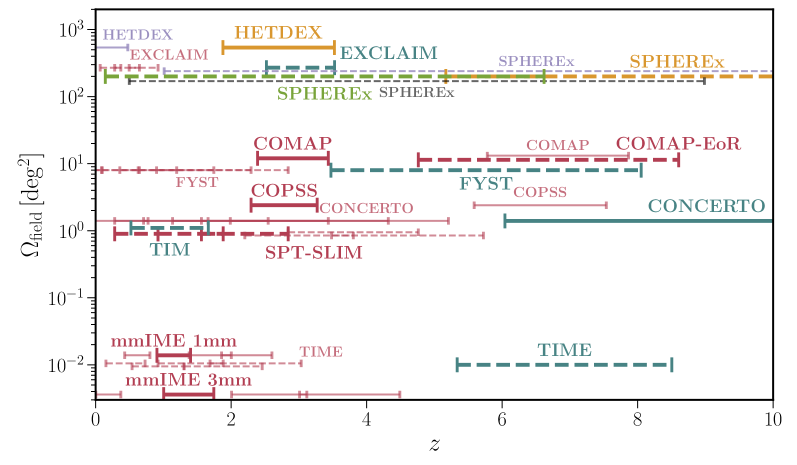
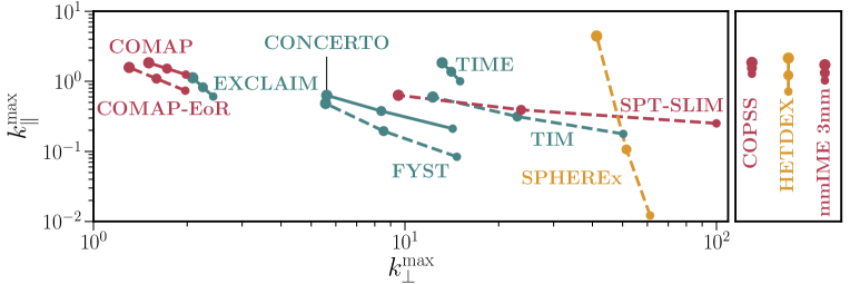
Figure 3: Current experimental landscape of LIM, including a representative list of ongoing and funded LIM surveys, denoting the targeted (thick) and interloper (thin, semitransparent) lines with different colors. Top: redshift range and total sky coverage (summing different observed patches when required) probed by each experiment. In some cases, the nominal sky coverage is slightly modified to ease the reading of the figure. Bottom: maximal line-of-sight and transverse wavenumbers accessible by each experiment with their main target emission lines, given the spectral and angular resolutions. We show values for the minimum, mean and maximum redshifts (marked by increasing size of the marker). The separate bottom panel contains experiments with significantly higher angular resolution.

Eventually, a third generation of LIM experiments will map huge volumes by either covering large sky fractions, like one of the proposed surveys for AtLAST 2020SPIE11445E..2FK , using high-sensitivity wide-bandwidth instruments (e.g. CDIM Cooray:2016hro ; 2019BAAS…51g..23C , COMAP-ERA COMAP:2021nrp ), or both (see ESA Voyage-2050 proposal Silva:2019hsh ; Delabrouille:2019thj ). Such flagship missions will truly unravel the potential of LIM Kovetz:2019uss .

We hope these optimistic arguments about the prospects of LIM provide ample motivation for the reader to indulge further in this review as it goes into more detail. However, it is important to bear in mind that LIM also presents a different set of challenges compared to other observables, including limitations due to thermal detector noise, contamination from continuum emission or interloper lines (spectral lines redshifted to the observed frequencies from other cosmological volumes than that of the target lines), and degeneracies between astrophysics and cosmology. These various traits and the methods proposed to address them will be covered in depth in the following sections of this review.

The outline of the review is as follows. We present an introduction to the primary emission lines targeted by LIM experiments in Sec. 2, and discuss different strategies to model their intensities in Sec. 3. After fully introducing LIM, we survey the prospects of this technique to improve our understanding of astrophysics and cosmology in Sec. 4. We then lay out the formalism for describing the statistical properties of line-intensity maps as well as the potential of cross-correlations with external observables in Secs. 5 and 6, respectively. We close the review with brief concluding remarks in Sec. 7.

2 Lines

A variety of galactic emission lines ranging from the microwave to the ultraviolet (UV) bands can be used to probe different phases of the IGM and ISM, and to study the various astrophysical processes shaping the host galaxies 2019ARA&A..57..511K . Line-intensity maps are connected to the emission from stars in different ways. Stellar emission ionizes and heats the ISM, which absorbs part of the UV radiation and re-emits it in the infrared 2012ARA&A..50..531K ; Madau:2014bja . Thus, as we discuss in Sec. 3, the relation between the UV and infrared luminosities is empirically related to the stellar mass or the UV-continuum spectral index Heinis:2013dsa ; 2016ApJ…833…72B ; 2020ApJ…902..112B . The stellar emission and infrared re-emission determine the ionization and photo-dissociation structure of the galaxy, triggering (directly or through cascades of events) the luminosity of the lines that LIM experiments target, as we detail below.

In this Section, we briefly introduce the main target lines for LIM following an increasing order in frequency, starting in the sub-millimeter range. In Fig. 4 we show examples of galactic spectra from the sub-millimeter to the near-UV.

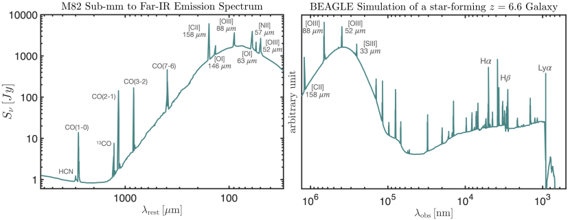
Figure 4: Left: M82 emission spectrum, at rest-frame wavelengths. Adapted from Ref. Wilson:2006cn . Right: A model spectral energy distribution from the BEAGLE simulation 2016MNRAS.462.1415C , at the observed wavelengths, of a star-forming galaxy at redshift $z\!=\!6.6$. Adapted from Ref. 2018ApJ…859…84H . We highlight some of the main lines targeted by LIM experiments, from CO(1-0) to Ly$\alpha$.

2.1 Carbon Monoxide (CO)

CO is the most common molecule in the Universe besides diatomic molecular hydrogen (H₂) and is the most widely-used tracer of molecular gas 1987ApJ…319..730S ; Dame:2000sp ; Walter:2003zh ; 2011MNRAS.412.1913I ; 2011MNRAS.415…32S ; Carilli:2013qm . Its rotational line emissions, at a ladder of frequencies $\nu_{J\rightarrow J-1}=J\times 115.27\,{\rm GHz}$ (or wavelengths $\lambda=2.6/J\,{\rm mm}$) for $(J\rightarrow J-1)$ transitions, are among the brightest in galactic spectra and can be efficiently observed by terrestrial telescopes targeting the sub-mm wavelength range (including the higher rotational lines that originate from high-redshift sources).

In principle, the CO(1-0) luminosity from virialized molecular clouds is linearly related to the cloud H₂ mass Narayanan:2011zm ; 2012ARA&A..50..531K ; Bolatto:2013ks ; 2015ARA&A..53..583H (provided the volume covered by molecular clouds is small enough so that the emission from one cloud is not absorbed by another 1986ApJ…309..326D ; Bolatto:2013ks ), which can be used to estimate the amount of stellar mass and the star-formation rate in galaxies Tacconi:2020wdz . However, the CO emission is very sensitive to the environment 2012A&A…541A..58L , depending on various factors such as metallicity Genzel:2011cw ; Popping:2013ixa ; 2022arXiv220406937S , gas temperature and density Krumholz:2011mq , the existence of a starburst phase Downes:1998vm ; Narayanan:2005xj , and the destruction of CO by cosmic rays Papadopoulos:2011kb ; 2015ApJ…803…37B .

All this makes the interpretation of CO LIM observations as a proxy for cosmic molecular abundance challenging Breysse:2021ecm , although there are ways to tighten this relationship. For example, luminosity ratios between different CO lines provide useful constraints on the physical conditions in the gas Solomon:2005xc . There is also potential to scrutinize the CO to H₂ relation directly using LIM of hydrogen deuteride, which may be observable during reionization with future instruments Breysse:2021utr . Another interesting target is the ¹³CO isotopologue at $\nu_{\rm rest}=110\,{\rm GHz}$ Breysse:2016opl ; cross-correlating ¹³CO and ¹²CO from the same sources provides an estimate of the gas density, as the former saturates at a much higher column density. Finally, due to similar critical densities, fine-structure lines of CI are highly correlated with CO lines independently of the environment, providing an alternative tracer of the molecular gas 2015A&A…578A..95I ; Jiao:2017knu ; 2018ApJ…869…27V ; 2019A&A…624A..23N , which can also be targeted by LIM Sun:2020mco ; Chung:2022lpr ; Bethermin:2022lmd and used to break degeneracies related with gas temperatures, excitation states and column densities.

As it has the lowest frequency among bright emission lines and is quite far from the HI line, observations of the CO(1-0) line are not prone to contamination from foreground interloper lines. The main culprit, HCN Breysse:2015baa , is quite weak in comparison Chung:2017uot (see Fig. 4). However, higher CO rotational lines can be mixed with lower ones, and many of them are strong interlopers for [CII] measurements at high-redshift.

2.2 Ionized Carbon [CII]

Atomic and ionic fine-structure lines in the infrared are important drivers of the cooling process of interstellar gas Carilli:2013qm . The [CII] $158\,{\mu\rm{m}}$ fine-structure line, mostly emitted from dense photo-dissociation regions in the outer layer of molecular clouds Stacey:2010ps , is the brightest among them Tielens:1985st ; 1991ApJ…373..423S ; Wolfire:2022dbc (see Fig. 4). There are studies indicating that the [CII] emission can also trace molecular gas 2018MNRAS.481.1976Z , even outperforming CO(1-0) for high-redshift low-metallicity galaxies 2022arXiv220305316V , and recent works suggest that a small but non-negligible fraction of the [CII] radiation may be emitted from ionized gas phases 2015A&A…575A..17H ; 2017ApJ…845…96C ; 2019A&A…626A..23C .

Assuming that galactic dust converts the vast majority of the UV and optical radiation it absorbs into infrared luminosity, and that only a remainder fraction is applied to photo-electric heating, the [CII] luminosity is proportional to the heating rate and to the fraction of atomic gas. Thus, [CII] provides a very natural target for LIM experiments to trace the star-formation history Suginohara:1998ti ; DeLooze:2011uw ; Herrera-Camus:2014qba , and due to its brightness, it is especially targeted at high redshifts. However, the tight relationship between the [CII] line and infrared luminosities yields a much larger scatter at high redshifts compared to what is observed at lower redshifts. Possible explanations 2019MNRAS.489….1F ; 2022arXiv220508905B include a large population of galaxies undergoing starbursts 2015ApJ…813…36V , low metallicities 2015ApJ…813…36V ; 2017ApJ…846..105O ; 2018A&A…609A.130L , and intense radiation fields in compact galaxies that photo-evaporate molecular clouds Gorti:2002xqa ; 2017MNRAS.471.4476D ; 2019MNRAS.487.3377D , regulating the [CII] luminosity 2017MNRAS.467.1300V . The effects of these processes are degenerate in the [CII] luminosity, but cross-correlating [CII] maps with observations of other far-infrared, CO, optical or UV lines, or with the cosmic infrared background (CIB), will help break the degeneracies.

The frequency of the [CII] line lies just above the ladder of CO lines, hence it suffers from their contamination as foreground line-interlopers Breysse:2015baa . Other atomic fine-structure lines (such as ionized oxygen and nitrogen or neutral carbon) also contaminate the [CII] line-intensity maps, but typically less severely.

2.3 Other Atomic Fine-Structure lines

Besides the carbon lines, other far–infrared fine-structure lines that can be used to probe ISM physics include silicon [SIII] $18\,{\rm\mu m}$ and $33\,{\rm\mu m}$, oxygen [OI] $63\,{\rm\mu m}$, [OIII] $52\,{\rm\mu m}$ and $88\,{\rm\mu m}$, and nitrogen [NII] $122\,{\rm\mu m}$ and $205\,{\rm\mu m}$. These lines and the ratios between them and other lines such as [CII] provide additional means to measure the electron density, excitation temperatures, gas pressure, metallicity, ionization parameter, the hardness of the ionizing radiation and the properties of both the neutral and ionized gas phases Serra:2016jzs ; 2019ARA&A..57..511K ; 2019ApJ…887..142S ; 2020MNRAS.499.3417Y ; 2021MNRAS.504..723Y ; Padmanabhan:2021tjr ; Padilla:2022asq .

For example, although [OIII] requires hard ionizing radiation and is typically weaker than [CII], in certain environments such as AGN and early galaxies it can in fact be brighter Carilli:2013qm (see Fig. 4). High [OIII]/[CII] ratios can hint at a [CII] deficit Laporte:2019rbp , but can also result from underestimation of [CII] emission in targeted observations as its emission tends to be more extended than [OIII] Carniani:2020ldd . Another example involves [NII], a tracer of regions of ionized hydrogen; the [NII] line luminosities depend on the electron density, the ionized-gas temperature, and the nitrogen-to-hydrogen abundance ratios 2015ApJ…814..133G ; 2016ApJ…826..175H .

2.4 Optical and ultraviolet hydrogen lines

Several key hydrogen lines such as Ly$\alpha$, H$\alpha$ and H$\beta$, emitted in the UV and optical and redshifted to wavelengths down to the infrared (see Fig. 4), provide another set of important targets of multiple LIM experiments.

Hydrogen recombinations following ionization by young stars and AGN, as well as collisional excitations from shock heating and cold accretion, can result in Ly$\alpha$ line emission, the most energetic line emission from star-forming galaxies Ouchi:2020zce . As they traverse the ISM and IGM, Ly$\alpha$ photons get repeatedly absorbed and re-emitted by neutral hydrogen. This multiple scattering disperses their directions and frequencies Santos:2003pc and increases the probability that they get absorbed by galactic dust. Thus, galaxy metallicity and dust content both have a direct impact on the observed Ly$\alpha$ emission Ouchi:2020zce . In general, the escape fraction of Ly$\alpha$ photons decreases with higher star-formation rate (which is associated with higher dust abundance Santini:2013yfa ), and increases, for high-redshift galaxies, with their redshift. As higher redshifts are probed, Ly$\alpha$ emission, especially through its escape fraction, provides an effective tracer of the neutral gas abundance. This is especially true for the dimmer emission from neutral circumgalactic and intergalactic media, which eventually become the tail of the EoR, and are more accessible with LIM Steidel:2011ey ; Zheng:2010tw . Hence, intensity maps of localized and extended Ly$\alpha$ emissions correlate with star-forming lines at the center of the ionizing sources, e.g. CO and [CII] Beane:2018pmx ; Moriwaki:2019dbg , as well as with the HI line from regions surrounding the bubbles Sobacchi:2016mhx .

The lower frequency hydrogen lines H$\alpha$ and H$\beta$ are emitted from the same sources as Ly$\alpha$ as a result of the ensuing radiative cascade of Ly$\alpha$ excitations. They are also susceptible to dust extinction, but much less than Ly$\alpha$ 2017arXiv171109902S . Roughly three times brighter than H$\beta$ 2006agna.book…..O , H$\alpha$ provides a fairly direct probe of star formation Kennicutt:1998zb ; Ly:2006hx ; Saito:2020qxq and can also be used in cross-correlation. For example, using LIM to measure the ratio between HeII (1640 ${\rm\AA}$) and H$\alpha$ towards cosmic dawn redshifts, $z\lesssim 20$, can constrain the initial mass function of Pop III stars Visbal:2015sca ; Parsons:2021qyw , as these produce more HeII ionizing photons than metal enriched stars Schaerer:2001jc .

Although the UV hydrogen lines have a series of interlopers Fonseca:2016qqw ; Gong:2020lim (see Fig. 4), the resolution required for these high-frequency observations typically allows separating between the target and interloper lines Breysse:2015baa ; Pozzetti:2016cch ; 2017arXiv171109902S . Some of these metal interlopers, such as [OII] 373.7 nm, [OIII] 495.9 nm and 500.7 nm, and [NII] 655.0 nm, provide faithful tracers of the star formation rate at low redshifts Kennicutt:1998zb ; Ly:2006hx ; Villa-Velez:2021ojy . Moreover, the [OII] doublet in particular can yield precise redshifts for galaxies observed with low integration times as is critical for the emission-line galaxy samples of eBOSS Raichoor:2017nuz and DESI Raichoor:2020jcl .

2.5 Preliminary detections

Risking a subsection that will quickly become obsolete, we briefly summarize the preliminary detections of LIM to date, to provide context for what follows.

CO(1-0) at redshifts $1\!<\!z\!<\!5$ has been the target line for several pathfinder LIM experiments. The first $\sim\!2\sigma$ detection of its shot-noise power at redshift $z\!\sim\!3$ was achieved by the COPSS survey using data from the Sunyaev-Zel’dovich Array Keating:2015qva ; Keating:2016pka . This was followed by a stronger $\sim\!4\sigma$ detection by mmIME Keating:2020wlx , using data from ALMA 2019ApJ…882..138D ; 2019ApJ…882..139G and ACA Scoville:2006vq . Recent work Keenan:2021uue showed the promise of cross-correlating CO(1-0) with galaxy surveys (and obtained preliminary upper limits at $z\sim 3$).

The first [CII] LIM measurement, at $2\sigma$ confidence-level, was obtained via cross correlation between maps from the Planck High Frequency Instrument and high-redshift catalogs of quasars and luminous red galaxies (LRGs) Pullen:2017ogs , with an improved methodology yielding a $\sim 4\sigma$ detection Yang:2019eoj . The detected excess above the CIB, stellar radiation reprocessed as infrared continuum emission by the dust Hauser:2001xs ; Kashlinsky:2004jt ; Wu:2016vpb , appears to be consistent with collisional excitation models of [CII] emission, where the intensity is proportional to the collisional rate, which depends on the gas density and temperature.

The Ly$\alpha$ LIM signal has been searched for using stacking Niemeyer:2022vrt and cross correlation between source redshift catalogs and maps expected to include residual Ly$\alpha$ emission from the same sources. First attempts to cross correlate BOSS quasar catalogs with BOSS LRG spectra proved challenging BOSS:2015ids ; Croft:2018rwv ; Renard:2020mfg . More recently, a $\sim\!3\sigma$ detection was reported using stacking of Subaru/HSC narrow-band images at $z\sim 6$ around resolved bright Ly$\alpha$ emitters Kakuma:2019afo .

3 Modeling

LIM experiments measure the specific intensity $I$ per unit of observed frequency $\nu_{\rm obs}$, which can be derived from the line-luminosity density $\rho_{\rm L}$ per comoving volume. We can transform $\rho_{\rm L}$ into flux volume density dividing by $4\pi D_{L}^{2}$, which is in turn converted to specific intensity by transforming the comoving volume element to solid angle and observed frequency elements as ${\rm d}A/{\rm d}\Omega=D_{M}^{2}$ and ${\rm d}\chi/{\rm d}\nu_{\rm obs}=c(1+z)/H\nu_{\rm obs}$, respectively. In the explanation above, $D_{L}$ is the luminosity distance, $D_{M}$ is the comoving angular diameter distance, $\chi$ is the comoving radial distance, $c$ is the speed of light and $H(z)$ is the Hubble expansion rate. However, experiments covering frequencies below some tens of GHz usually employ the brightness temperature $T=c^{2}I/(2k_{B}\nu_{\rm obs}^{2})$ using the Rayleigh-Jeans relation. Therefore, we can use

$$I(z)=\frac{c}{4\pi\nu H(z)}\rho_{\rm L}(z)\,,\qquad{\rm or}\qquad T(z)=\frac{c^{3}(1+z)^{2}}{8\pi k_{\rm B}\nu^{3}H(z)}\rho_{\rm L}(z)\,,\quad$$ (1)

where $\nu$ is the line rest-frame frequency, and $k_{\rm B}$ is the Boltzmann constant.

Contrary to the HI emission before reionization, the spectral lines we focus on in this review originate in galaxies and the IGM within dark matter halos, given their relation to emission from young, bright stars. Therefore, it is fair to identify the line sources with galaxies, although in some cases, especially for the Ly$\alpha$ line, radiative transfer extends the emission profile far beyond the size of the halo 2021ApJ…916…22K ; 2022ApJ…929…90L ; 2021arXiv210809288K ; Niemeyer:2022vrt . $\rho_{\rm L}$ can be obtained using either a luminosity function or a direct relation $L(M,z)$ between the halo mass and the line luminosity at each redshift. For instance, the mean luminosity density can be obtained as

$$\langle\rho_{\rm L}\rangle(z)=\int{\rm d}ML(M,z)\frac{{\rm d}n}{{\rm d}M}(M,z)=\int{\rm d}LL\frac{{\rm d}n}{{\rm d}L}(z)\,,$$ (2)

where ${\rm d}n/{\rm d}M$ and ${\rm d}n/{\rm d}L$ are the halo-mass and line-luminosity functions. From expressions like this and through the connection to the halo distribution, it is possible to derive summary statistics to describe line-intensity maps and extract astrophysical and cosmological information. In Sec. 5 we will focus on one- and two-point statistics (the voxel-intensity distribution (VID) and the power spectrum, respectively). We will use $L(M)$ in what follows unless otherwise stated, since it allows for more direct physical modeling of the line intensity, although all of our expressions can be easily adapted to the luminosity function. To model the line intensity, we need to relate it with the galaxy properties (this can be compressed in the $L(M)$ relation thereafter).

There are two main approaches to estimating the line intensity in connection to the galaxy properties. One possibility relies on empirical scaling relations fit to observations. Another involves theory-motivated relations, that may range from analytic derivations to semi-analytic models to fully-fledged hydrodynamic simulations. For the sake of usability, empirical relations can also be calibrated on the results of these simulations rather than observations. Each approach has its own benefits and flaws, and a robust understanding of the astrophysical dependence of LIM will likely require a combination of both.

In Fig. 5 we show the results of using empirical scaling relations to model the intensities as a function of redshift for the LIM target lines discussed above.

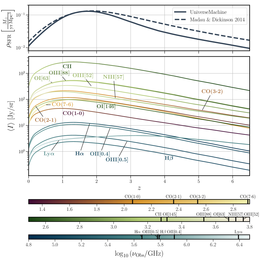
Figure 5: Bottom: Microwave, infrared, optical and UV spectral lines (rest-frame frequencies marked with vertical bars in the colorbar) mean intensity as function of redshift, obtained using scaling relations from the infrared luminosity and star formation rates Kennicutt:1998zb ; 2016ApJ…829…93K ; Spinoglio:2011ug ; DeLooze:2014dta ; 2017ApJ…835..273G ; COMAP:2018svn . We use star-formation rates and quenching fractions from Refs. Behroozi:2012iw ; Behroozi:2019kql assuming a mean-preserving logarithmic scatter of $0.3\,{\rm dex}$ in the star-formation rate to halo mass relation. Top: Star-formation rate density Behroozi:2019kql ; Madau:2014bja . Line-intensity ratios evolve with redshift; current observational constraints apply at specific redshifts and are uncertain by up to one order of magnitude.

3.1 Empirical Scaling relations

Scaling relations are most useful when they connect line luminosities to quantities that are relatively easy to observe, such as the infrared luminosity, or to general galaxy properties that can be inferred from observations, like the star-formation rate. For instance, since optical hydrogen and oxygen lines are good star-formation tracers, their luminosities are in tight linear relations with the star-formation rate, as shown in observations Kennicutt:1998zb ; Ly:2006hx ; 2011ApJ…737…67M ; Villa-Velez:2021ojy , and based on stellar evolutionary tracks, ionizing emissivity and recombination rates.

Meanwhile, the emission of the [CII] line correlates with both the far-infrared emission from dust 1985ApJ…291..755C ; 1991ApJ…381..200W and with star formation 1991ApJ…373..423S ; DeLooze:2014dta ; 2017ApJ…834…36H . Low-redshift DeLooze:2014dta ; Herrera-Camus:2014qba and high-redshift 2015Natur.522..455C ; Carniani:2020ldd ; 2020A&A…643A…3S observational studies obtained a nearly linear correlation between [CII] luminosity and the star-formation rate, without redshift dependence, while numerical simulations 2015ApJ…813…36V ; 2017ApJ…846..105O ; 2020MNRAS.492.2818L ; Pallottini:2022inw and semi-analytic models 2018A&A…609A.130L ; 2019MNRAS.482.4906P predict a weak dependence on redshift. Observational correlations between the [CII] luminosity and star-formation rates in the local Universe DeLooze:2014dta are found to still apply at high redshifts 2015Natur.522..455C ; Chung:2018szp ; ALPINETeam:2019arv ; 2020ApJS..247…61F . This is surprising, since massive high-redshift galaxies correspond to a much higher [CII] surface brightness regime than the populations observed at low-redshift 2016ApJ…833…71A ; 2019MNRAS.489….1F ; Pizzati:2020bqq , and may change with more observations.

Fine-structure lines, as dust-cooling emission lines, are correlated to the infrared luminosity Spinoglio:2011ug ; 2017ApJ…846…32D . The situation is very similar for the ladder of CO rotational lines, with the subtle difference of observational results being reported in terms of the $L^{\prime}$ pseudo luminosity, expressed in K km/s pc² units. There is rich literature on relations for the ground transition Daddi:2010nn ; Carilli:2013qm ; 2014ApJ…794..142G ; Sargent:2013sxa ; 2015A&A…577A..50D . The intensity of the other CO rotational transitions is determined by the spectral line energy distribution, which shows large variety between different studies 2015ApJ…801…72R ; 2016ApJ…829…93K ; 2017A&A…608A.144Y ; 2018A&A…620A..61C ; 2020A&A…641A.155V ; 2020ApJ…902..109B ; 2020ApJ…889..162L . The spectral-line energy distribution depends largely on the galaxy type 2016ApJ…829…93K , with the CO to infrared-luminosity relations typically lower in starburst galaxies compared to main-sequence galaxies Aalto:1995au ; Genzel:2010na ; Daddi:2010nn ; 2015ApJ…810L..14L , mainly due to differences in star-formation to molecular mass ratios.

As an example, let us briefly describe the procedure to obtain $L(M)$ for the CO lines. The first step is to assign a star-formation rate $\rm{SFR}(M,z)$ to any halo of mass $M$ at redshift $z$. The mean $\rm{SFR}(M,z)$ is often parameterized with a double power law Silva:2014ira ; Fonseca:2016qqw ; 2017ApJ…835..273G , or using more involved fitting functions Behroozi:2019kql . As empirical relations are not ubiquitous and there is significant variability in the populations considered, it is quite common to add a characteristic log-normal scatter. A typical value is $\sigma_{\rm SFR}\sim\!0.3\,{\rm dex}$ Behroozi:2012iw . In the second step, we assume that the infrared luminosity and the star-formation rate are correlated, and adopt an ansatz $L_{\rm IR}=1.72\times 10^{-10}{\rm SFR}/M_{\odot}{\rm yr}^{-1}L^{-1}_{\odot}$ Kennicutt:1998zb . Finally, we use a power-law relation between infrared and CO luminosities

$$\log L_{\rm IR}=\alpha_{J}\log L^{\prime}_{\rm CO(J\rightarrow J-1)}+\beta_{J}\,,$$ (3)

where $\alpha_{J}$ and $\beta_{J}$ depend on the transition and the data used to calibrate the correlation, and $L_{\rm CO(J\rightarrow J-1)}/L_{\odot}=4.9\times 10^{-5}J^{3}(L^{\prime}_{\rm CO(J\rightarrow J-1)}/\rm K\ km\ s^{-1}\ pc^{2})$. We then add another log-normal scatter $\sigma_{\rm L}\sim\!0.3\,{\rm dex}$. To summarize, we assign

$$L_{\rm CO(J\rightarrow J-1)}\Bigg{(}L_{\rm IR}\Big{(}{\rm SFR}(M,z),\sigma_{\rm SFR}\Big{)},\alpha_{J},\beta_{J},\sigma_{\rm L}\Bigg{)}$$ (4)

to any halo of mass $M$ at redshift $z$. We note that this relation can be made more accurate if the stellar mass $M_{*}$ in the halo can be estimated. In this case we can use the observed infrared-to-ultraviolet excess (IRX$\equiv L_{\rm IR}/L_{\rm UV}$) to account for the stellar light that is not reprocessed into infrared photons

$$\text{SFR}=K_{\rm UV}L_{\rm UV}+K_{\rm IR}L_{\rm IR}\,,\qquad\qquad\text{IRX}=\left(\frac{M_{*}}{M_{s}}\right)^{x}\,,$$ (5)

where $K_{\rm UV}=2.5\times 10^{-10}\ M_{\odot}{\rm yr}^{-1}L^{-1}_{\odot}$ and $K_{\rm IR}=1.73\times 10^{-10}\ M_{\odot}{\rm yr}^{-1}L^{-1}_{\odot}$ (following Ref. Madau:2014bja ), and $x=0.97^{+0.17}_{-0.17}$, $\log_{10}(M_{s}/M_{\odot})=9.15^{+0.18}_{-0.16}$, and a log-normal scatter of $\sigma_{\rm IRX}=0.2$ dex 2020ApJ…902..112B is included. This improved relation downweights the contribution from halos with low star-formation rate Wu:2016vpb .

Ly$\alpha$ emission involves more complicated radiative transfer, including dust absorption without photo-ionization, recombination line emission absorbed by dust, and ionizing photons escaping the galaxy without any ionization events or being absorbed by HI regions without triggering recombination line emission. For the purposes of Ly$\alpha$ intensity mapping, these processes can be merged and modeled as an escape fraction, which depends significantly on the environment and is all but unconstrained observationally. However, current measurements show two general trends COMAP:2018svn : the escape fraction increases monotonically with redshift, and it decreases with higher star-formation rate. One can then use a general function depending on redshift and star-formation rate satisfying these limiting trends COMAP:2018svn , or other parameterizations based on constraints to the escape fraction and other contributions to the Ly$\alpha$ intensity Fonseca:2016qqw ; Silva:2012mtb .

Using empirical relations provides a fast method to predict the line intensities, taking into consideration observational constraints and without relying on theoretical priors, hence involving a more agnostic prediction accounting for potentially unknown astrophysics. Empirical approaches can be very powerful in resolving occasional discrepancies between theory-based estimates. On the other hand, the observations used to calibrate these scaling relations span a very specific redshift interval, which either limits their application to LIM analyses or forces to extrapolate the results to other redshifts. The latter option may result in very inaccurate estimations. One example of this is the ground transition of CO Breysse:2014uia , as highlighted in Ref. COMAP:2021rny . Using low-redshift data Carilli:2013qm ; 2016ApJ…829…93K one finds best-fit values around $\alpha_{1}\approx 0.1\beta_{1}+1.19$ Li:2015gqa for the relationship between the parameters in Eq. (3), while using high-redshift observations, such as the COLDz luminosity functions at $z\sim 2.4$ Riechers:2018zjg , yields $\alpha_{1}=0.67$ and $\beta_{1}=4.90$ LC_paper .

3.2 Theory-motivated approaches

There are three main types of theory-motivated approaches to model line intensities, which can be distinguished by their numerical complexity: analytic models, semi-analytic models and hydrodynamic simulations.

Analytic models aim to relate line luminosities to the ISM properties, which requires modeling the phases of the galaxy and the relative abundances of each of its main components. There are many ways to achieve this goal, but all of them start with modeling the stellar radiation. Some options 2019ApJ…887..142S use CIB models Shang:2011mh and relations between star-formation rate and infrared luminosities Kennicutt:1998zb . The gas-to-dust mass ratios can be obtained from the dust model using observation-based calibrations of the dust-grain emission 2014A&A…566A..55P , in addition to the total hydrogen mass, which is distributed between neutral, ionized and molecular hydrogen 2020ApJ…902..111W . Finally, the metallicity is obtained from the hydrogen and dust masses, assuming a constant dust-to-metal ratio (which can be obtained from hydrodynamic galaxy formation simulations 2019MNRAS.490.1425L ). Other options 2015JCAP…11..028M ; 2019MNRAS.489….1F model the ionization and photo-dissociation structure properties of a galaxy to determine its ionized and neutral regions as a function of the galaxy’s stellar emission and ionization field. From this point, it is possible to estimate line luminosities in a general way that can be applied to both low and high redshift galaxies.

Analytic models are forced to make simplifying assumptions about the processes involved in the line emission for the sake simplicity. Concrete interstellar conditions can be taken into account with photo-ionization simulation codes 2017RMxAA..53..385F ; Krumholz:2013qza ; 2020MNRAS.494.1919L , but in order to fully track galaxy properties, numerical hydrodynamic simulations are required. These simulations evolve astrophysical properties self-consistently in each simulation cell, according to specific robust underlying physical baryonic models. However, the increased complexity sets an upper limit on the volume of the simulation as a tradeoff; if the simulation volume is too large, more of the baryonic physics implemented may rely on sub-grid models. The results of these simulations (see e.g., Hopkins:2013vha ; McAlpine:2015tma ; 2015ApJ…813…36V ; 2017ApJ…846..105O ; Nelson:2018uso ; Dave:2019yyq ; 2020MNRAS.492.2818L ; Pallottini:2022inw ) can be post-processed to consistently predict the intensity of several lines 2021arXiv211105354S . Furthermore, the THESAN project Kannan:2021xoz has recently modeled several emission lines at reionization using a radiation-magneto-hydrodynamic simulation that self-consistently models hydrogen reionization and the properties of the galaxies and active galactic nuclei Kannan:2021ucy . In practice this relies on several ad-hoc assumptions, such as a fixed ionization parameter, for instance.

Nonetheless, hydrodynamic simulations are computationally very expensive, which imposes significant limitations on their use and flexibility. Semi-analytic models, in turn, offer a compromise between analytic approaches and hydrodynamic simulations 2015ARA&A..53…51S . This approach dynamically evolves dark matter and baryons in a cosmological context, using motivated approximations relying on sub-grid physics to treat star formation and baryonic feedback (see e.g., Refs. Somerville:1998bb ; Lu:2013mxa ; 2013MNRAS.431.3373H ; Somerville:2008bx ; 2015MNRAS.453.4337S ; 2016MNRAS.462.3854L ; Croton:2016etl ). The free parameters of these recipes are calibrated to match global observational quantities to observations or numerical simulations. Then, the results can be used to simulate multiple line luminosities for each galaxy Lagos:2012sv ; 2016MNRAS.461…93P ; Dumitru:2018tgh ; 2018A&A…609A.130L ; 2019MNRAS.482.4906P ; 2020ApJ…905..102L , and match it with a halo catalog within a lightcone from N-body simulations to build a mock LIM observation 2021ApJ…911..132Y .

It has been shown that hydrodynamic simulations and semi-analytic models are generally in good agreement 2015ARA&A..53…51S , which motivates the use of semi-analytic models to generate simulated line-intensity maps. Finally, the results obtained from hydrodynamic simulations or semi-analytic models can be empirically summarized in scaling relations of the same form as the ones discussed in the previous subsection to facilitate their use 2018A&A…609A.130L ; 2020ApJ…905..102L ; 2022ApJ…929..140Y .

4 Prospects

From the discussion in the two previous sections, it is evident that LIM serves both as a means of gathering statistical information about the Universe at high redshifts, and as a statistical probe of astrophysical evolution throughout the history of the Universe. As such, its prospects are unique and far-reaching. While current preliminary detections and upper limits have limited constraining power, forthcoming LIM observations will be able to yield invaluable information about galaxy formation and evolution, cosmology and fundamental physics. Here we describe some of the most motivated proposals to fulfill these goals, discussing the inherent sensitivity of LIM to the relevant signatures.

4.1 Astrophysics

As emission from all sources is aggregated in line-intensity maps, component separation and information extraction become challenging and highly model-dependent. However, there is hope to mitigate this limitation by improving our understanding of the processes triggering different line emissions through line cross-correlations and combinations with external observables, as well as by comparing with targeted detailed observations of selected samples (see Sec. 6). The prospects for LIM to deepen our knowledge about astrophysics are mostly based on improving our understanding of the connection between the IGM and ISM properties and the line intensities, discussed in Sec. 3. Below we (somewhat artificially) distinguish between the potential of LIM to probe the star-formation history, the properties of the ISM, and the process of reionization.

4.1.1 Star-formation history

Star-formation rates are a proxy for the stellar emission of young stars, which are one of the main drivers of galaxy evolution, as well as for determining its chemical evolution and gas reservoirs (in a circular, self-regulated, process 2011ARA&A..49..373B ; Fu:2012qt ; Carilli:2013qm ). Most of our current understanding of the high-redshift star-formation rate comes from optical and UV observations of stellar light and emission lines from the hot ionized gas in the ISM, but around half of the starlight is re-processed by dust Casey:2018hlz and only the brightest galaxies can be detected by galaxy surveys Sargent:2013sxa ; Kistler:2013jza ; 2017MNRAS.467.1222H , which leads to great uncertainties. Observations and analytic studies support a universal, power-law relation between the star-formation rate and gas content of the galaxy Kennicutt:1998zb ; Leroy:2008kh ; Daddi:2010nn ; Fu:2010qc ; Krumholz:2011jm ; 2015ApJ…805…31L ; 2019ApJ…872…16D ; 2021ApJ…908…61K , depending on stellar feedback and other astrophysical processes 2019MNRAS.488.4753D , but its potential redshift evolution is unknown Santini:2013yfa ; 2021ApJ…908…61K . LIM can trace: (i) the cold molecular gas where stars form using CO lines Righi:2008br ; Mashian:2015his ; Breysse:2016szq ; Breysse:2016opl ; Breysse:2015saa ; Li:2015gqa (with isotopologue line ratios sensitive to the initial mass function 2019ApJ…879…17B ); (ii) the actual instantaneous star formation with optical hydrogen and oxygen lines 2013ApJ…763..132S ; 2017ApJ…835..273G ; 2018MNRAS.475.1587S ; (iii) the impact of star formation on the surrounding gas with fine-structure lines Silva:2014ira ; Yue:2015sua ; (iv) and the redshifted radiation from Pop III stars with helium and hydrogen lines Visbal:2015sca ; Parsons:2021qyw ; Sun:2021drn . All this, while surveying large enough volumes to provide ample statistics.

Finally, Ref. Sun:2022qrd proposes to constrain the global star-formation law from the amplitude of a scale-dependent bias sourced by baryon fluctuations on baryon acoustic oscillations (BAO) scales Barkana:2010zq ; Angulo:2013qp ; Schmidt:2016coo ; Soumagnac:2016bjk (still to be detected in galaxy clustering Soumagnac:2016bjk ; Soumagnac:2018atx ). The bias depends on the line luminosity (see Sec. 5), hence the target contribution can be isolated from the ratio of the power spectra of two lines. Non-linear clustering, which affects the BAO amplitude and the bias terms (see Ref. Chen:2020ckc ), makes this approach challenging.

4.1.2 The properties of the ISM

The general properties of the ISM are expected to evolve substantially with redshift. The first galaxies are thought to be small, compact, both metal and dust poor, with a young stellar population, undergoing frequent mergers, exposed to a much weaker background radiation, etc. Moreover, early-galaxy populations are expected to be significantly less homogeneous, requiring larger samples to study global quantities.

As stated above, LIM can probe many different scales and phases in the ISM and IGM thanks to its access to multiple emission lines and the sensitivity to all emitters. Molecular gas can be probed with the CO lines, especially combining CO isotopologues to obtain a better picture of high-density clouds Breysse:2016opl ; 2018Natur.558..260Z , and potentially using rotational transitions of hydrogen deuteride to target the earliest, ultra-low-metallicity galaxies Bromm:2013iya . Since the total gas mass is indirectly constrained by CIB measurements, combining HI (to separate between neutral and molecular gas abundances) and CO reduces the uncertainties in the molecular gas mass to CO luminosity relation, though uncertainties dependent on gas temperature and metallicity remain Blain:2002ec ; 2019ApJ…887..142S . These degeneracies are further reduced by adding [CII] intensity maps to the analysis, due to their indirect dependence on the abundance of molecular gas.

Meanwhile, the HII regions can be studied with the [NII] lines and their ratios, which are sensitive to the electron density and temperature 2019ApJ…887..142S ; 2015ApJ…814..133G ; 2017ApJ…846…32D . At the same time, Ly$\alpha$ can probe the circumgalactic medium, especially its ionization state and the gas density distribution 2013ApJ…763..132S ; Pullen:2013dir ; Comaschi:2015waa , with improved sensitivity if cross-correlated with [CII] Comaschi:2016soe .

LIM excels in probing the properties of the ISM and IGM in two more aspects. First, it is possible to study the ISM and IGM of specific galaxy populations by cross-correlating line-intensity maps with the corresponding sub-sample of galaxies under consideration 2019MNRAS.490..260B . Secondly, most of the baryon content in the Universe is spread throughout warm low density gas regions Fukugita:1997bi ; Cen:1998hc ; while this gas is undetectable by galaxy surveys, it can be probed with LIM, complementing other techniques such as the Sunyaev-Zel’dovich effect ACTPol:2015teu ; deGraaff:2017byg , as we discuss in Sec. 6.

4.1.3 The process of reionization

Reionization is the last phase transition the Universe has undergone, yet the EoR remains mostly unexplored by direct observations. This is when the first stars and galaxies formed, and together with accreting black holes, gradually ionized the neutral gas surrounding them Barkana:2000fd ; 2013fgu..book…..L ; 2016ARA&A..54..761S . A simplistic view of the epoch of reionization depicts the IGM as a two-phase fluid, with ‘bubbles’ of ionized gas growing around the first luminous sources with neutral gas filling the space in-between. Hence, the discussion of the previous subsection also applies to the study of reionization, when framed for lower metallicities and younger galaxies.

Star-formation and IGM models are very sensitive to assumptions related to the ISM and the whole population of star-forming galaxies 2011ARA&A..49..373B . This population can be efficiently probed with intensity maps of emission lines related to star formation Gong:2011mf ; Padmanabhan:2018yul . In turn, Ly$\alpha$ probes some combination of the sources and the IGM Pullen:2013dir ; 2013ApJ…763..132S ; Visbal:2018dsi . Thus, cross-correlation between these lines or with HI, which traces the neutral gas, will significantly improve our ability to map and understand reionization and the interplay between ionizing sources and the IGM Lidz:2008ry ; Gong:2011mf ; Lidz:2011dx ; Dumitru:2018tgh ; Padmanabhan:2021tjr ; Cox:2022hxl , mitigating limitations due to foregrounds Lidz:2011dx and assumptions about escape fractions for ionizing photons 2011ApJ…730…48P . Finally, to probe the evolution of reionization, one can use the anti-symmetric cross-correlations of HI and other lines Sato-Polito:2020qpc ; Zhou:2020hqh ; Zhou:2020woq , which evolve oppositely as reionization progresses.

4.2 Cosmology

It is important to place the discussion of the prospects for cosmology with LIM experiments targeting emission lines related with star formation in the suitable context. LIM, especially for these lines, is still in the pathfinder stage, with current-generation experiments probing small volumes, as shown in Fig. 3. Hence, it is evident that LIM needs the time to evolve and mature before it can be competitive with flagship CMB experiments such as CMB-S4 CMB-S4:2016ple and galaxy surveys such as Euclid Amendola:2016saw and DESI DESI:2016fyo .

Nevertheless, even if cosmology continues to be dominated by the CMB and galaxy surveys for the near future, LIM observations grant access to regimes and scales that are out of reach for other observables; examples include access to redshifts in-between volumes probed by galaxy surveys and CMB experiments, and the sensitivity to the integrated emission from the faintest astrophysical sources in the Universe, which form in less massive collapsed objects than those traced by galaxy surveys. This is what makes LIM a unique and complementary cosmological probe with great promise to constrain physics beyond $\Lambda$CDM. In addition, combining multi-line observations over the same redshift volumes and using cross-correlations with other observables can be used to mitigate cosmic variance via the multi-tracer technique Seljak:2008xr ; McDonald:2008sh .

Below we discuss the intrinsic benefits that the LIM particularities offer for cosmology. While some of the target signatures may be degenerate with astrophysics, actual line intensities will affect LIM’s potential through their impact on the signal-to-noise ratio of the measurements. Quantitative forecasts (under a given set of assumptions) can be found in Ref. Karkare:2022bai .

4.2.1 Dark matter

LIM can probe small-scale matter clustering in two ways: through small-scale clustering measurements and through its dependence on the abundance of collapsed objects. Hence, LIM is sensitive to the effects of dark matter models that change the statistics of biased tracers of small-scale dark matter fluctuations, such as self-interacting dark matter Tulin:2017ara , models of dark matter-baryon scattering Dvorkin:2013cea , and ultra-light axion dark matter Hlozek:2014lca . The high sensitivity of LIM to models that modify the halo mass function has been demonstrated for observations before reionization Munoz:2019hjh ; Jones:2021mrs ; Sarkar:2022dvl and at lower redshifts Bauer:2020zsj ; Libanore:2022ntl ; Sabla2022 .

As it collects all incoming photons, LIM is naturally suitable for searches of exotic sources of radiation. Furthermore, LIM’s spectral resolution provides additional information on the spectral energy distribution of this radiation, allowing to separate between different processes. In the case of dark matter radiative decays, the resulting radiation effectively produces an emission line that will show up in LIM experiments as an interloper Creque-Sarbinowski:2018ebl . Techniques proposed to model and deal with line-interloper contamination (see Sec. 5) can be adapted to target and maximize the signal from these decays Bernal:2020lkd ; Shirasaki:2021yrp . For example, forecasts indicate that LIM will be one of the most sensitive probes of a possible coupling between electron-volt-scale axions and photons Adams:2022pbo , which may weigh in on potential explanations Bernal:2022wsu for the recent excess measurement of the cosmic optical background Lauer:2022fgc . Similar strategies can be applied to look for neutrino decays Bernal:2021ylz , the detection of which would hint at physics beyond the standard model of particle physics.

4.2.2 Light relics

Neutrinos act like free-streaming particles and cannot be confined to regions smaller than their free-streaming scale. This scale grows until neutrinos become non relativistic ($z\sim 100-200$), after which it begins to shrink. Thus, neutrinos suppress matter clustering in a scale- and time-dependent manner Lesgourgues:2013sjj .

LIM will yield clustering measurements across a very wide redshift range, complementing those from galaxy surveys at lower redshifts and tracking the redshift evolution of the neutrino-induced scale-dependent suppression. Tracking the evolution of this dependence can break parameter degeneracies between the CMB and large-scale structure probes Yu:2018tem , especially between the sum of neutrino masses and the amplitude of the primordial power spectrum, the CMB optical depth to reionization, and the dark energy equation of state Hannestad:2005gj ; Liu:2015txa ; Allison:2015qca . LIM measurements split into several redshift bins will be highly sensitive to the neutrino mass Bernal:2019jdo ; MoradinezhadDizgah:2021upg . Similar promise can be expected for other models involving light relics, such as dark matter decaying into lighter dark matter particles FrancoAbellan:2021sxk . Finally, LIM can contribute to constraining $N_{\rm eff}$, the number of effective relativistic degrees of freedom in the early Universe, by extending searches for changes in the BAO phase Baumann:2017lmt ; Baumann:2019keh to higher redshifts and larger volumes.

4.2.3 Dark energy

The cosmic expansion history is strongly constrained at $z\lesssim 2.5$ from type-Ia supernovae Brout:2022vxf and BAO measurements from galaxy surveys eBOSS:2020yzd . At earlier times, we rely on extrapolations of an expansion determined by a matter-dominated Universe, which reproduce existing measurements Planck:2018vyg ; ACT:2020gnv . The lack of direct measurements may hide deviations from $\Lambda$CDM predictions that are degenerate with other parameters, such as “tracking” dynamic dark-energy models, predicted by certain modified gravity theories (see e.g. Refs. Raveri:2017qvt ; Raveri:2019mxg ).

The tomographic access to $z\gtrsim 2.5$ that LIM experiments provide will allow us to directly measure the expansion history of the Universe through BAO measurements Chang:2007xk ; Bernal:2019gfq ; Karkare:2018sar . While percent-level BAO measurements at $z>3$ will require stage-3 LIM experiments, current-generation experiments have the potential to return the first robust direct constraints on the expansion history at such redshifts (although anisotropies produced by line broadening may hinder the realization of the full potential of this cosmological probe COMAP:2021rny ).

LIM BAO measurements will bridge the gap between $H(z)$ constraints from galaxy surveys and CMB experiments, even for agnostic parameterizations Bernal:2016gxb ; Verde:2016ccp ; Bernal:2021yli , which will weigh in on the Hubble constant tension Freedman:2021ahq ; DiValentino:2021izs . Moreover, pre-recombination deviations from $\Lambda$CDM proposed to solve the tension (see e.g. Refs. Karwal:2016vyq ; Poulin:2018cxd ; Niedermann:2019olb ) affect the matter clustering also through perturbations of the new fields Smith:2019ihp . This significantly impacts the halo mass function, introducing deviations that increase with redshift Klypin:2020tud . LIM, which depends on the high-redshift halo mass function, will be especially sensitive to this effect. Finally, tomographic growth-rate constraints with LIM clustering measurements Bernal:2019jdo will also improve constraints on modified gravity theories Ferreira:2019xrr .

4.2.4 Inflation

The quintessential smoking gun for inflation is the detection of primordial gravitational waves, often parameterized by the tensor-to-scalar ratio. Currently, the most promising venue to detect such signatures is through primary $B$-modes in the CMB polarization Kamionkowski:2015yta . However, inflationary features may lie beyond the description of the tensor-to-scalar ratio Achucarro:2022qrl ; some examples include primordial non-Gaussianity Meerburg:2019qqi , isocurvature perturbations Bartolo:2001rt , deviations from the almost scale-independent primordial power spectrum, spectral-index running Munoz:2016owz , power-spectrum oscillations Zeng:2018ufm , etc., all of which can be constrained with large-scale structure measurements. Detecting or ruling out these features will provide invaluable information about inflation. As a leading example, a sizable local-type primordial non-Gaussianity can only be produced in scenarios with multi-field inflation Maldacena:2002vr ; Creminelli:2004yq ; dePutter:2016trg .

Primordial non-Gaussianity generically modifies the abundance of collapsed objects Matarrese:2000iz , induces scale dependence to the linear bias Dalal:2007cu ; Matarrese:2008nc , and modifies the bispectrum Creminelli:2003iq ; Alishahiha:2004eh ; Cheung:2007st ; Senatore:2009gt ; Chen:2006nt ; Holman:2007na ; Karagiannis:2019jjx . These effects are usually apparent at large scales and grow with redshift, hence making LIM a very promising way to improve current sensitivities MoradinezhadDizgah:2018zrs ; MoradinezhadDizgah:2018lac ; Bernal:2019jdo ; MoradinezhadDizgah:2020whw ; Liu:2020izx ; Chen:2021ykb . Furthermore, the possibility to study and cross-correlate several lines in tomography up to high redshifts will help break degeneracies with compensated isocurvature perturbations Sato-Polito:2020cil , bias uncertainties Barreira:2022sey , and to reduce the limitations related with cosmic variance Oxholm:2021zxp ; Seljak:2008xr ; McDonald:2008sh ; Fonseca:2015laa ; Alonso:2015sfa .

5 Formalism

LIM fluctuations are a biased tracer of matter density perturbations, but also depend on various astrophysical processes, which introduces additional non-Gaussianity in the line-intensity maps with respect to other tracers of the large scale structure. With the objective of recovering as much information as possible from line-intensity maps, several summary statistics have been proposed to exploit LIM observations. Below we will focus on the power spectrum (the formalism of which can be extended to configuration space or to higher order statistics), and on the voxel intensity distribution. We refer the reader to more focused references for other summary statistics such as the mapping of Ly$\alpha$ polarization Mas-Ribas:2020wkz , or the lensing of line-intensity maps Foreman:2018gnv ; Maniyar:2021arp .

Going back to Eq. (1), we define the conversion factors $X_{\rm LI}$ and $X_{\rm LT}$ between intensity or temperature to luminosity density as $\rho_{\rm L}=I/X_{\rm LI}=T/X_{\rm LT}$. Expressions below are valid for both conventions, with the appropriate factor.

5.1 Power spectrum

5.1.1 Intrinsic signal

The LIM power spectrum has two main components: the clustering part, which follows the matter power spectrum, and a shot noise contribution due to the sources of the line not being a continuous field. The simplest formulation of the anisotropic power spectrum in redshift space is

$$P(k,\mu)=\left[X_{\rm LI}\int{\rm d}M\frac{{\rm d}n}{{\rm d}M}Lb_{\rm h}F_{\rm rsd}(k,\mu)\right]^{2}P_{\rm m}(k)+X_{\rm LI}^{2}\int{\rm d}M\frac{{\rm d}n}{{\rm d}M}L^{2}\,,$$ (6)

where all quantities also depend on redshift (and halo mass $M$, with the exception of $X_{\rm LI}$), $\mu\equiv\boldsymbol{k}\cdot\boldsymbol{k}_{\parallel}/k^{2}$ is the cosine of the angle between the Fourier mode $\boldsymbol{k}$ and its component $\boldsymbol{k}_{\parallel}$ along the line of sight, $k=\lvert\boldsymbol{k}\lvert$, $b_{\rm h}$ is a mass-dependent linear halo bias relating halo-number and matter perturbations, $F_{\rm rsd}$ is a factor encoding the effect of redshift-space distortions, $P_{\rm m}(k)$ is the linear matter power spectrum, ${\rm d}n/{\rm d}M$ is the halo mass function, and we have assumed Poissonian shot noise. Note that any eventual scatter in the relations determining the luminosity function $L(M)$ must be taken into account in the integrals over the halo mass functions above. The clustering and shot noise terms depend on the first and second moments of the luminosity distribution, respectively. This means that, although the shot noise power spectrum often yields a considerably higher detection significance than the clustering component (especially for small-volume surveys), a significant detection of both components is required to break degeneracies in the $L(M)$ relation 2019MNRAS.490.1928Y .

The $F_{\rm rsd}$ factor includes the Kaiser effect Kaiser:1987qv , relevant at large scales, and a function suppressing the power spectrum at scales below a characteristic scale related to the halo pairwise velocity dispersion $\sigma_{\rm pv}$, to empirically reproduce the fingers-of-God effect Jackson:1971sky . Using for instance a Lorentzian function,

$$F_{\rm rsd}(k,\mu)=\frac{1+\frac{f\mu^{2}}{b_{\rm h}(M)}}{1+0.5\left(k\mu\sigma_{\rm pv}(M)\right)^{2}}\,,$$ (7)

where $f$ is the growth rate.

The linear power spectrum, Eq. (6), does not provide a good prediction of LIM clustering at small scales. This regime can be better modeled using the halo model Cooray:2002dia

$$\begin{split}P(k,\mu)=&\left[\left(X_{\rm LI}\int{\rm d}M\frac{{\rm d}n}{{\rm d}M}Lb_{\rm h}F_{\rm rsd}(k,\mu)\mathcal{U}(k)\right)^{2}P_{\rm m}(k)+\right.\\ &+\left.X_{\rm LI}^{2}\int{\rm d}M\frac{{\rm d}n}{{\rm d}M}L^{2}\mathcal{U}^{2}(k)\right.\Bigg{]}+P_{\rm shot}\,,\end{split}$$ (8)

where $\mathcal{U}$ is the Fourier transform of the density profile (here assumed spherical) of a halo of mass $M$, and $P_{\rm shot}$ is the shot noise power spectrum from Eq. (6). The first and second terms in the square brackets correspond to the two-halo and one-halo terms, respectively. Further non-linearities, in the matter power spectrum and in the bias expansion, can be accounted for (see Ref. MoradinezhadDizgah:2021dei for an example using effective field theory in the context of CO and [CII] intensity mapping). Furthermore, the contributions of each of the galaxies within a halo can be modeled: the halo occupation distribution model Kravtsov:2003sg can be generalized to LIM fluctuations rescaling the line luminosity of central and satellite galaxies accordingly 2019ApJ…887..142S . In this case, the one-halo term includes the correlations between satellite and central galaxies and an additional shot noise term related with the number of emitters per halo Schaan:2021gzb .

So far, we have assumed a Dirac-delta line profile. However, velocity dispersion of the gas from which the lines are emitted broadens the emission line. In practice, this effect is similar to the fingers-of-God, but related to velocity dispersion within a single halo rather than pairwise velocity dispersion. In this case, the rotation velocity greatly dominates over thermal velocities. Assuming a Gaussian line profile, the gas rotation velocity $v$ broadens the line, resulting in a full-width half maximum of $\theta^{\nu}_{\rm FWHM}=\nu v(M)/c$. Unless $v(M)/c\ll 1$ (in practice, smaller than the spectral resolving power of the experiment, see below) the line broadening must be taken into account. The physical scale corresponding to the standard deviation of the broadened line-profile is $\sigma_{v}(M)=v(M)(1+z)/{H(z)\sqrt{8\log 2}}$. The effect of the line broadening in the power spectrum is similar to the spectral resolution limit, but in this case the suppression depends on the halo mass and affects differently the clustering and shot noise contributions COMAP:2021rny :

$$\begin{split}P_{\rm broad}=&\left[X_{\rm LI}\int{\rm d}M\frac{{\rm d}n}{{\rm d}M}Lb_{\rm h}F_{\rm rsd}e^{-k^{2}\sigma_{v}^{2}(M)\mu^{2}/2}\right]^{2}P_{\rm m}(k)+\\ +&X_{\rm LI}^{2}\int{\rm d}M\frac{{\rm d}n}{{\rm d}M}L^{2}e^{-k^{2}\sigma_{v}^{2}(M)\mu^{2}}\,.\end{split}$$ (9)

The power spectrum statistic suffers from degeneracies between the effect of the cosmological parameters and the dependence on astrophysics, that persist even after optimal reparameterizations Bernal:2019jdo . These degeneracies can be broken to a large degree by using mildly non-linear scales in the LIM power spectrum Castorina:2019zho ; MoradinezhadDizgah:2021dei , combining it with higher order statistics Gil-Marin:2014pva ; Sarkar:2019ojl , employing phase statistics Wolstenhulme:2014cla ; Byun:2020hun , or using external priors on the astrophysical parameters COMAP:2018svn ; 2021arXiv211105354S .

5.1.2 Observational effects

LIM observations measure intensities as function of frequencies and angular positions on the sky, but three-dimensional clustering measurements need spatial distances. This requires interpreting observed frequencies as redshifts (introducing projection effects for interloper lines, see below) and using a fiducial cosmology to transform these into distances. Assuming a background expansion that differs from the true one adds an artificial anisotropy in the map, which is known as the Alcock-Paczynski effect Alcock:1979mp . This effect, in conjunction with the BAO standard ruler, is used to extract the expansion history of the Universe from clustering measurements Eisenstein:2003qy ; Blake:2003rh ; Seo:2003pu with great precision eBOSS:2020yzd in a model independent way Carter:2019ulk ; Bernal:2020vbb .

The observed power spectrum is also limited by the spectral and angular resolutions of the experiment and the volume probed. Generally, a Gaussian beam with full-width half maximum $\theta_{\rm FWHM}=1.22c/\nu_{\rm obs}D$ for a dish with diameter D, is assumed. The angular and spectral resolutions correspond to physical distance scales transverse to and along the line of sight as

$$\sigma_{\perp}=D_{\rm M}\frac{\theta_{\rm FWHM}}{\sqrt{8\log 2}}\,,\qquad\sigma_{\parallel}=\frac{c\delta\nu(1+z)}{H\nu_{\rm obs}}\,,$$ (10)

respectively, where $\delta\nu$ is the minimum separation in frequency considered. The resolution limit results in a smearing of the observed line-intensity map, which can be modeled with a convolution in configuration space over a window function $W_{\rm res}$. Noting that $W_{\rm res}=W_{\rm res}^{\perp}W_{\rm res}^{\parallel}$ we have that, in Fourier space,

$$W_{\rm res}^{\perp}=\exp\left\{-k^{2}\sigma_{\perp}^{2}(1-\mu^{2})\right\}\quad{\rm and}\quad W_{\rm res}^{\parallel}=\begin{cases}&\exp\left\{-k^{2}\sigma_{\parallel}^{2}\mu^{2}\right\}\,,\\ &{\rm sinc}\left(\frac{k\mu\sigma_{\parallel}}{2}\right)\,,\end{cases}$$ (11)

depending on whether single Gaussian channels are used or many of them are stuck for $\delta\nu$ not related with spectral resolution.

Similarly, the volume probed is determined by the total area $\Omega_{\rm field}$ of the sky surveyed and the frequency band of the experiment. We can model the loss of modes beyond the size of the observed volume and the effect of variable observing conditions with the mask $W_{\rm vol}$. The Fourier transform of the observed intensity fluctuations $\delta I(\boldsymbol{x})$ is then

$$\begin{split}\delta\tilde{I}(\boldsymbol{k})&=\int{\rm d}^{3}\boldsymbol{x}e^{-i\boldsymbol{k}\boldsymbol{x}}W_{\rm vol}(\boldsymbol{x})\int{\rm d}^{3}\boldsymbol{x}^{\prime}W_{\rm res}(\boldsymbol{x}-\boldsymbol{x}^{\prime})\delta I(\boldsymbol{x}^{\prime})=\\ &=\int\frac{{\rm d}^{3}\boldsymbol{q}}{(2\pi)^{3}}\delta I(\boldsymbol{k}-\boldsymbol{q})W_{\rm res}(\boldsymbol{k}-\boldsymbol{q})W_{\rm vol}(\boldsymbol{q})\,,\end{split}$$ (12)

which results in an observed power spectrum

$$\tilde{P}(\boldsymbol{k})=\int\frac{{\rm d}^{3}\boldsymbol{q}}{(2\pi)^{3}}W^{2}_{\rm vol}(\boldsymbol{q})W^{2}_{\rm res}(\boldsymbol{k}-\boldsymbol{q})P(\boldsymbol{k}-\boldsymbol{q})\,,$$ (13)

where the tilde denotes observed quantities. The anisotropic power spectrum cannot be measured, but it is possible to measure the Legendre multipoles directly, using e.g., the Yamamoto estimator Yamamoto:2005dz . The observed LIM power spectrum multipoles are Chung:2019iim ; Bernal:2019jdo

$$\begin{split}\tilde{P}_{\ell}(k)=\frac{2\ell+1}{2}\int_{-1}^{1}{\rm d}\mu\tilde{P}(k,\mu)\mathcal{L}_{\ell}(\mu),\end{split}$$ (14)

where $\mathcal{L}_{\ell}$ is the Legendre polynomial of degree $\ell$. In Fig. 6, we show the monopole and quadrupole of the intrinsic and observed power spectra, varying the scatter of the star-formation rate to halo mass relation.

Figure 6: CO power spectrum monopole (left) and quadrupole (right) at $z=2.9$. We show the true total power spectrum (dashed), the observed one (solid), and the shot noise power spectrum (dotted), varying the dispersion $\sigma_{\rm SFR}$ of the star formation rate to halo mass relation, assuming a beam of $\theta_{\rm FWHM}=1^{\prime}$, spectral resolution of $\delta\nu=31.25$ MHz, and a cylindrical volume corresponding to 200 deg² and 7.7 GHz ($\Delta z=1$).

5.1.3 Covariance

Experimental limitations also introduce an instrumental white-noise floor in the LIM observations. The total noise variance per antenna per observed voxel when only the autocorrelation between antennas is considered is

$$\sigma_{{\rm N},I}^{2}=\frac{\sigma_{\rm pix}^{2}}{N_{\rm feeds}N_{\rm pol}t_{\rm pix}}\,,\qquad\sigma_{{\rm N},T}^{2}=\frac{T_{\rm sys}^{2}}{N_{\rm feeds}N_{\rm pol}\delta\nu t_{\rm pix}}\,,$$ (15)

for intensities and temperatures, respectively, where $\sigma_{\rm pix}$ is the noise equivalent intensity (NEI), $T_{\rm sys}$ is the instrument system temperature, $N_{\rm feeds}$ is the number of detectors per antenna, $N_{\rm pol}=1,2$ is the number of polarizations the detectors are sensitive to, and $t_{\rm pix}$ is the observing time per pixel. One can also include the frequency dependence on the noise per voxel Chung:2022lpr .

The noise power spectrum is then $P_{\rm N}=\sigma_{\rm N}^{2}V_{\rm vox}/N_{\rm ant}$, where $V_{\rm vox}$ is the volume of the voxel and $N_{\rm ant}$ the number of antennas used. Assuming Gaussianity and neglecting mode coupling, the power spectrum variance per $\mu$ and $k$ bin is

$$\tilde{\sigma}^{2}(k,\mu)\equiv\left[\tilde{P}(k,\mu)+P_{\rm N}\right]^{2}/N_{\rm modes}\,,$$ (16)

where $N_{\rm modes}=V_{\rm field}k^{2}\Delta k\Delta\mu/(8\pi^{2})$ is the number of modes observed per bin in a volume $V_{\rm field}$. Small volumes may be affected by higher cosmic variance due to limited Poisson sampling from luminosity functions 2020ApJ…904..127K . The total covariance matrix for the power-spectrum multipoles is composed of the subcovariance matrices between $\ell$ and $\ell^{\prime}$ multipoles Bernal:2019jdo ,

$$\tilde{C}_{\ell\ell^{\prime}}(k)=\frac{\left(2\ell+1\right)\left(2\ell^{\prime}+1\right)}{2}\times\int_{-1}^{1}{\rm d}\mu\tilde{\sigma}^{2}(k,\mu)\mathcal{L}_{\ell}(\mu)\mathcal{L}_{\ell^{\prime}}(\mu).$$ (17)

5.1.4 Cross correlation

As discussed in previous sections, cross-correlations of different lines reduce the impact of contaminants and allow for more detailed astrophysical analyses. Furthermore, the cross-correlations of three lines may be used to reconstruct their auto-power spectra free of contaminants Beane:2018dzk . The cross-power spectrum between two lines can be computed following the formalism above, substituting all quadratic terms by the product of the contribution from each line and including their correlation coefficient Pullen:2012su ; Wolz:2017rlw ; 2019MNRAS.490..260B ; 2019ApJ…887..142S ; Liu:2020izx . At large enough scales, intensity fluctuations are completely correlated. Astrophysical dependence results in different $L(M)$ relations, which changes the line bias and may affect the correlation coefficient at intermediate and small scales. Thus, the correlation coefficient between two lines is generally scale dependent.

One effective way to formalize the inter-dependence between line luminosities and the host halo is through conditional luminosity functions Yang:2002ww , as proposed in Ref. Schaan:2021gzb . The conditional luminosity function models the mean number of galaxies in a halo of mass $M$ with luminosities $L_{1},\dots,L_{p}$ for lines $1,\dots,p$. A complete modeling of the conditional luminosity function applied to the halo model self-consistently returns the one-halo term and shot noise contributions and accounts for any scale dependence of the correlation coefficient Schaan:2021gzb . However, modeling the conditional luminosity function is very challenging since, as discussed in previous sections, the modeling of each independent line at this point is already quite uncertain.

The variance per $\mu$ and $k$ bin of the cross-power spectrum of two line-intensity maps is

$$\tilde{\sigma}^{2}_{XY}=\frac{1}{2}\left(\frac{\tilde{P}_{XY}^{2}}{N_{\rm modes}}+\tilde{\sigma}_{X}\tilde{\sigma}_{Y}\right),$$ (18)

where $\tilde{\sigma}_{X}$ and $\tilde{\sigma}_{Y}$ are computed following Eq. (16) for each of the lines.

5.1.5 Angular power spectrum

The angular power spectrum neglects the line-of-sight information within a redshift bin, but may be useful in cases with low spectral resolutions or to cross-correlate signals from different redshifts. Moreover, it is measured in observed coordinates and directly considers a curved sky, which avoids theoretical systematics related with wide-angle effects for wide surveys Szalay:1997cc ; Raccanelli:2010hk ; Castorina:2017inr ; Yoo:2013zga . Tomographic angular analyses can better model the frequency evolution of the noise and the telescope beam, and can incorporate the experience from CMB analyses, such as the pseudo-$C_{\ell}$ technique Hivon:2001jp ; Tristram:2004if .

The angular power spectrum of maps $X$ and $Y$ as function of harmonic multipole $\ell$ at redshift bins $z_{i}$ and $z_{j}$ is given by

$$\mathcal{C}_{\ell}^{X,Y}(z_{i},z_{j})=4\pi\int\frac{{\rm d}k}{k}\Delta_{\ell}^{X,z_{i}}(k)\Delta_{\ell}^{Y,z_{j}}(k)P_{\rm prim}(k)\,,$$ (19)

where $P_{\rm prim}$ is the dimensionless primordial matter power spectrum and the transfer function $\Delta_{\ell}$, accounting for the angular resolution and ignoring observational masks, is

$$\Delta_{\ell}^{X,z_{i}}(k)=\int{\rm d}z\mathcal{W}^{X}(z,z_{i})\Delta_{\ell}^{X}(k,z_{i})\exp\left\{-\frac{\ell(\ell+1)(\theta_{\rm FWHM}^{X})^{2}}{16\log 2}\right\}\,,$$ (20)

where $\mathcal{W}$ is a normalized function centered on $z_{i}$ to delimit the redshift bin and $\Delta_{\ell}^{X}$ includes all the contributions to the observed perturbations of tracer $X$; for instance, the linear intrinsic clustering contribution corresponds to $\langle I_{X}b_{X}\rangle\mathcal{T}j_{\ell}(k\chi)$, where $\mathcal{T}$ is the matter transfer function, and $j_{\ell}$ is the $\ell$-th order spherical Bessel function. The corresponding shot noise

$$C_{\ell}^{X,Y,{\rm shot}}=\int\frac{{\rm d}z}{\chi^{2}}\mathcal{W}^{X}(z,z_{i})\mathcal{W}^{Y}(z,z_{j})\delta_{ij}^{\rm K}\int{\rm d}M\frac{{\rm d}n}{{\rm d}M}L_{X}(M)L_{Y}(M)\,,$$ (21)

where $\delta^{\rm K}$ is the Kronecker Delta, must also be included. The observed angular power spectrum $\tilde{\mathcal{C}}_{\ell}^{X,Y}$ also includes the contribution from the noise $N_{\ell}^{X}=\sigma_{\rm N,T}^{2}\delta\nu/(N_{\rm ant}\Delta_{i}\nu)\delta_{XY}^{\rm K}\delta_{ij}^{\rm K}=\sigma_{\rm N,I}^{2}/(N_{\rm ant}\Delta_{i}\nu)\delta_{XY}^{\rm K}\delta_{ij}^{\rm K}$, where $\Delta_{i}\nu$ is the frequency width of the $i$-th redshift bin. The covariance between the angular power spectra observed over a fraction $f_{\rm sky}$ of the sky is then

$${\rm Cov}\left[\mathcal{C}_{\ell,(i,j)}^{X,Y},\mathcal{C}_{\ell,(p,q)}^{X,Y}\right]=\frac{\tilde{\mathcal{C}}_{\ell,(ip)}^{X,X}\tilde{\mathcal{C}}_{\ell,(jq)}^{Y,Y}+\tilde{\mathcal{C}}_{\ell,(iq)}^{X,Y}\tilde{\mathcal{C}}_{\ell,(jp)}^{X,Y}}{(2\ell+1)f_{\rm sky}}\,,$$ (22)

where the subscripts in brackets denote the redshift bins. The effects of contaminants and mode coupling due to incomplete sky coverage can also be modeled under this framework, following e.g., Ref. Anderson:2022svu .

Spherical Fourier-Bessel analyses combine the main benefits of the three-dimensional and the angular power spectra, at the expense of numerical complexity. Ref. Liu:2016xzv developed a framework to analyze LIM clustering in this basis, including also observational effects.

5.2 Voxel intensity distribution

The voxel intensity distribution (VID), which is the histogram of measured intensities, is an estimator for the probability distribution function (PDF) $\mathcal{P}(I)$ of the line intensity within a voxel. The VID encodes information about the whole intensity distribution, or luminosity function, providing complementary information to the power spectrum (which only probes its mean and variance), as demonstrated in Ref. COMAP:2018kem ; Libanore:2022ntl . The intensity in a voxel is the sum of the intensities emitted by each of the $N_{\rm e}$ emitters it contains. If the line broadening is large enough, the contribution from an emitter may extend beyond the voxel, which can be accounted for with a window function Thiele:2020rig ; Bernal2022 .

The PDF of astrophysical sources is the sum of the conditional probabilities of having a given number of emitters in the voxel contributing to a total intensity Breysse:2016szq : $\mathcal{P}_{\rm astro}(I)=\sum\mathcal{P}_{N_{\rm e}}(I)\mathcal{P}_{\rm e}(N_{\rm e})$, where $\mathcal{P}_{\rm e}(N_{\rm e})$ and $\mathcal{P}_{N_{\rm e}}(I)$ are the PDFs of the number of emitters within a voxel and their total intensity, respectively. If there is no emitter in a voxel, the astrophysical intensity is null: $\mathcal{P}_{0}(I)=\delta_{D}(I)$. On the other hand, since the intensity is additive Breysse:2016szq , this can be written as a convolution

$$\mathcal{P}_{N_{\rm e}}(I)=(\underbrace{\mathcal{P}_{1}*\dotsc*\mathcal{P}_{1}}_{N_{\rm e}})(I)\,,\qquad\mathcal{P}_{1}(I)=\frac{V_{\rm vox}}{\bar{n}X_{\rm LI}}\left.\frac{{\rm d}n}{{\rm d}L}\right\lvert_{L=\rho_{L}(I)V_{\rm vox}}\,,$$ (23)

where $\bar{n}$ is the mean comoving number density of emitters and ‘$*$’ is the convolution operator.

The number of emitters in a voxel obeys a Poisson draw with its mean equal to the expected number of emitters in that specific voxel, which depends on clustering. Ref. Breysse:2016szq assumes that the emitter number count follows the matter distribution, approximated with a log-normal distribution 1991MNRAS.248….1C ; Kayo:2001gu .

Alternatively, $\mathcal{P}(I)$ can be explicitly expressed as a conditional probability depending on the emitter overdensity field $\delta_{\rm e}^{\rm v}$ smoothed over a voxel Sato-Polito:2022fkd . In this case, $\mathcal{P}_{\rm e}(N_{\rm e})$ is a Poisson distribution with space-dependent mean $N(\boldsymbol{x})=\bar{N}\left[1+\delta_{\rm e}^{\rm v}(\boldsymbol{x})\right]$. The average over realizations can be later performed by invoking the Ergodic hypothesis. Although these two derivations are equivalent under the same set of assumptions, the latter allows the derivation of an analytic covariance between the VID and the power spectrum Sato-Polito:2022fkd , which depends on the integrated bispectrum Chiang:2014oga of one power of the emitter overdensity and two of the intensity fluctuations. This analytic covariance is consistent with simulation-based covariances COMAP:2018kem . In general, the correlation between the two summary statistics cannot be neglected for low instrumental noises (achievable by the final stages of current-generation experiments), and it peaks for low intensities and small scales (until resolution or instrumental noise limits the measurement).

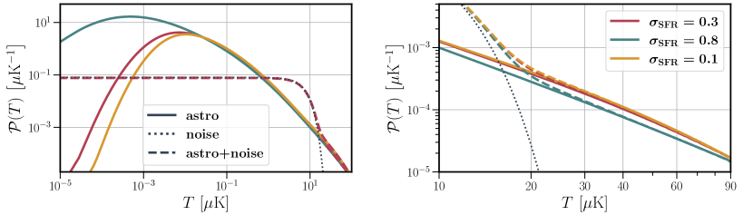
Figure 7: CO temperature PDF for the same cases as in Fig. 6. We show the PDF from the astrophysical contributions alone (solid), from the instrumental noise alone (dotted), and for their sum after mean subtraction (dashed); we assume $\sigma_{N}=5\,\mu{\rm K}$. The right panel zooms in on the tail of the PDF, which in practice is the only range from which it is possible to extract astrophysical information.

The observed intensity also includes the contribution from instrumental noise, with a PDF $\mathcal{P}_{\rm noise}$. The PDF for the total measured temperature in a voxel is then $\mathcal{P}_{\rm obs}=\left(\mathcal{P}_{\rm astro}*\mathcal{P}_{\rm noise}\right)(I)$. In the presence of foregrounds, or in case measuring absolute intensities is not possible, the ignorance about the zero point of the intensity PDF must be accounted for by considering only the PDF of the intensity perturbations: $\mathcal{P}_{\Delta}(\Delta I)\equiv\mathcal{P}(\Delta I+\langle{I}\rangle)$ Breysse:2016szq . We show the astrophysical and total PDFs in Fig. 7.

Finally, the predicted PDF must be connected to the observable, the VID $\mathcal{B}_{i}$. Using bins of width $\Delta I_{i}$,

$$\mathcal{B}_{i}=N_{\rm vox}\int_{I_{i}-\Delta I_{i}/2}^{I_{i}+\Delta I_{i}/2}\mathcal{P}_{\rm obs}(I){\rm d}I\,,$$ (24)

where $N_{\rm vox}$ is the total number of voxels in the survey. To estimate the covariance, a first approximation assumes that $\mathcal{B}_{i}$ follows a multinomial distribution Breysse:2016szq , with negligible contributions from cosmic variance in most cases Sato-Polito:2022fkd . However, there is physical covariance between different intensity bins COMAP:2018kem that needs to be modeled, which requires a different formalism to compute the two-point PDF Bernal2022 .

The VID can be useful in a variety of applications, besides direct parameter inference. For example, an extension of the VID formalism, in which the probability density distribution is conditioned on the number of detected galaxies in a voxel, has been proposed as a means to cancel out galactic foregrounds Breysse:2019cdw . Splitting the measured intensity into two contributions, $I=I_{1}+I_{2}$, where only $I_{1}$ is correlated with a field $y$, we can express the conditional PDF as

$$\mathcal{P}(I|y)=\mathcal{P}(I_{1}|y)*\mathcal{P}(I_{2}|y)=\mathcal{P}(I_{1}|y)*\mathcal{P}(I_{2})\,,$$ (25)

since $\mathcal{P}(I_{2}|y)\equiv\mathcal{P}(I_{2})$ by definition. Thus, the contributions from $I_{2}$ can be canceled out when comparing conditional PDFs for different values of $y$. An efficient way to do this in practice is with the ratio of the Fourier transform for different values of $y$. Taking $\mathcal{I}\equiv 2\pi/I$ as the Fourier conjugate of the intensity and $\breve{\mathcal{P}}(\mathcal{I}|y)$ as the Fourier transform of the conditional PDF,

$$\frac{\breve{\mathcal{P}}(\mathcal{I}|y_{1})}{\breve{\mathcal{P}}(\mathcal{I}|y_{2})}=\frac{\breve{\mathcal{P}}(\mathcal{I}_{1}|y_{1})\breve{\mathcal{P}}(\mathcal{I}_{2})}{\breve{\mathcal{P}}(\mathcal{I}_{1}|y_{2})\breve{\mathcal{P}}(\mathcal{I}_{2})}=\frac{\breve{\mathcal{P}}(\mathcal{I}_{1}|y_{1})}{\breve{\mathcal{P}}(\mathcal{I}_{1}|y_{2})}\,,$$ (26)

which is completely independent of the contributions of $I_{2}$. This ratio can be estimated using the ratio of conditional VIDs Breysse:2019cdw .

The VID is complementary to the power spectrum beyond its access to the non-Gaussian information in the map. While the power spectrum is more sensitive to cosmology, only depending on astrophysics through integrals of the luminosity function, the VID depends directly on the (convolutions of the) luminosity function, and is only sensitive to cosmology through the expected number of galaxies per voxel. Hence, combining the power spectrum and the VID can help break the degeneracy between cosmology and astrophysics COMAP:2018kem ; Sato-Polito:2022fkd ; Sabla2022 .

5.3 Continuum emission

Intensity mapping of star-formation lines suffers from different observational contaminants than HI observations. At higher frequencies, Galactic foregrounds are less significant and better behaved Planck:2016frx . The main source of continuum foregrounds is the CIB. It traces the same objects that LIM targets, but is subject to different astrophysical processes and blends together all radial information Shang:2011mh . This contribution is mixed with the continuum emission of foreground galaxies. After its removal, residual continuum foreground contamination is mostly contained in the lowest line-of-sight Fourier modes, especially for experiments with high spectral resolution Keating:2015qva ; Switzer:2015ria ; Switzer:2017kkz ; Switzer:2018tel , a limitation that may be partially lifted by applying neural networks Pfeffer:2019pca ; Moriwaki:2020bpr .

Uncorrelated continuum emission (from the Milky Way and foreground galaxies) cancels in cross-correlations between LIM and galaxy surveys. However, the correlated continuum emission (from the actual galaxies that LIM traces) prevails, which enables the reconstruction of the galaxy spectral energy distribution, combining line and dust emission Serra:2016jzs ; Cheng:2021wex .

5.4 Line interlopers

Line-interlopers can be challenging for LIM of star-formation lines, which are closer to each other in frequency. There are two main approaches to dealing with line interlopers: cleaning them from the observed maps, or modeling their contribution to avoid loss of signal and attempting to exploit the astrophysical and cosmological information encoded in their intensities.

Line-interlopers are usually sourced in different cosmic volumes than the target signal. Therefore, cross-correlating the map with an alternative tracer (e.g., galaxy surveys or the intensity of other spectral lines) of the cosmic volume from which the target signal comes leaves the interloper contribution out Lidz:2008ry ; Visbal:2010rz ; Gong:2011mf ; Chang:2015era ; Silva:2014ira ; Chang:2010jp ; Masui:2012zc ; BOSS:2015ids ; Comaschi:2016pad ; COMAP:2018svn ; Visbal2022 . A similar approach can be used for the VID, using conditional distributions Breysse:2019cdw ; 2021arXiv211105354S , as described above. These cross-correlations can later be used to reconstruct the auto power spectra Switzer:2013ewa ; Beane:2018dzk .

Another option involves the masking of voxels thought to be dominated by interloper contamination (including atmospheric lines for ground and balloon experiments). Masking can be either guided or blind. Guided masking 2018ApJ…856..107S ; 2021arXiv211105354S involves the use of external observations to identify interloper emitters. This approach cleans the interloper contribution from both bright and faint sources, minimizing the loss of information. Blind masking in turn can be used to clean the map in the absence of external observations. Assuming that the brightest voxels are likely dominated by the contribution from foreground interloper lines, as these typically come from lower redshift where galaxies tend to be more massive and more clustered, blind masking takes such voxels out to remove the brightest interloper contamination Visbal:2011ee ; Breysse:2015baa ; Gong:2013xda . Masking complicates the survey window and alters the bias and amplitude of the shot noise, since it downsamples the intrinsic line-luminosity function, which hinders the theoretical interpretation of the observations Visbal:2011ee .

The frequencies of the interlopers are known, which enables one to identify and characterize their contamination using spectral templates to fit the observed spectrum in each pixel map Cheng:2020asz . Knowledge about the interlopers can also be used to train deep learning models with simulations to separate components in the observed maps 2020MNRAS.496L..54M ; Moriwaki:2020bpr ; Moriwaki:2021yie . Each method can reconstruct the VID and the power spectrum of each component, respectively, and both are limited by the instrumental noise, resolution, and size of the survey.

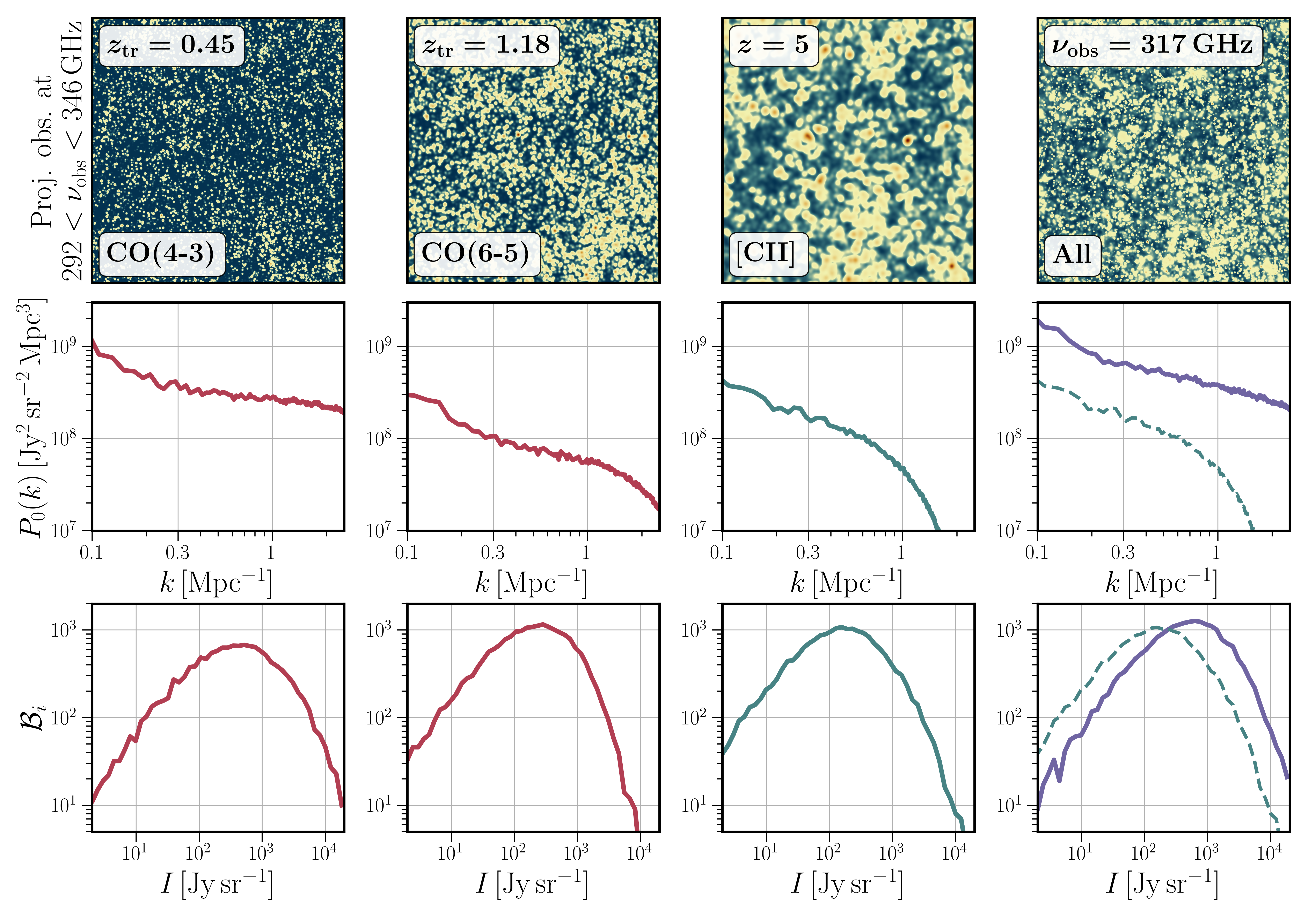
Figure 8: Simulated noisless intensity fluctuations observed in the frequency range 292-346 GHz, targetting the [CII] line and including the projected contributions from CO(4-3) and CO(6-5) as interlopers, coming from $z=0.45$ and $1.18$, respectively, but with three-dimensional spatial scales “wrongly” interpreted at $z=5$ (top panels). We also show the monopole of the power spectrum (middle panels) and the mean-subtracted VID (bottom panels). The three columns on the left show individual contributions from each line (CO lines in red, [CII] in blue), while the last column shows the sum of all contributions (in purple), with dotted lines showing the [CII]-only case to ease comparison. These results were obtained using the approach of Ref. LC_paper , assuming empirical relations from Refs. 2016ApJ…829…93K ; DeLooze:2014dta .

Nevertheless, the contribution from line interlopers contains astrophysical and cosmological information. Together with the problems introduced by the methods discussed above, this motivates the modeling of the interloper contributions. The misestimation of the line redshift introduces projection effects: strong, artificial anisotropic distortions in the three-dimensional cubes Gong:2013xda ; Lidz:2016lub ; 2017ApJ…835..273G ; Cheng:2016yvu ; Gong:2020lim . Projection effects in clustering statistics can be modeled similarly to the Alcock-Paczynski (AP) effect, with a slight modification of the rescaling parameters:

$$q_{\perp}=\frac{D_{M}(z_{\rm int})}{D_{M}(z_{\rm t})},\qquad q_{\parallel}=\frac{(1+z_{\rm int})/H(z_{\rm int})}{(1+z_{\rm t})/H(z_{\rm t})}\,,$$ (27)

where the subscripts ‘int’ and ‘t’ refer to the interloper and target line, respectively. Thus, the auto-power spectrum of the interloper contribution is $\tilde{P}_{\rm int}(k^{\rm infer}_{\parallel},k^{\rm infer}_{\perp})=\tilde{P}_{\rm int}(k_{\parallel}^{\rm meas}/q_{\parallel},k_{\perp}^{\rm meas}/q_{\perp})/(q_{\parallel}q_{\perp}^{2})$, where beam smoothing, the mask and other filtering effects must be applied at $z_{\rm int}$. Assuming no overlap in the volume probed by each line, the total measured power spectrum multipoles are

$$\tilde{P}_{\ell}^{\rm tot}(k^{\rm meas})=\tilde{P}_{\ell}^{\rm t}(k^{\rm meas},z_{\rm t})+\sum\tilde{P}^{{\rm int},i}_{\ell}(k^{\rm infer},z_{\rm int})\,.$$ (28)

Note that the impact of the rescaling due to projection effects is usually significantly larger than the AP effect. The covariance of the total power spectrum is computed following Eq. (17) at $z_{\rm t}$, using $\tilde{P}_{\ell}^{\rm tot}$ to calculate $\tilde{\sigma}^{2}$.

The contribution from interlopers also affects the measured VID, which can be modeled as an additional contribution to the PDF. In this case, the total measured intensity is $I=I_{\rm t}+\sum I_{{\rm int},i}+I_{\rm noise}$, hence the total VID is

$$\mathcal{P}_{\rm tot+\chi}=\left(\mathcal{P}_{\rm t}*\mathcal{P}_{\rm noise}*\mathcal{P}_{\rm all\,int}\right)(I)\,,$$ (29)

where $\mathcal{P}_{\rm all\,int}$ is the multiple convolution of the PDF for each interloper. We show an example of the contribution of interlopers to the power spectrum monopole and the VID in Fig. 8.

As mentioned above, the techniques to model known interlopers can also be used to look for exotic mono-energetic contributions to the intensity maps, such as radiative decays of dark matter and neutrinos Bernal:2020lkd ; Bernal:2021ylz .

5.5 Mocks

LIM modeling, the improvement of summary statistics to describe the map, and the development of techniques to deal with contaminants, all benefit from mock LIM observations. Contrary to analytic studies, mocks allow us to account for the whole distribution of galaxy properties and the scatter of scaling relationships. In addition, mocks account more accurately for non-linear clustering and allow for a more realistic inclusion of observational effects. For all these reasons, mocks are in practice the only way to fully account for the complexity and highly non-Gaussian nature of LIM, which has promoted their use as a gold standard in the field.

In most cases, LIM mocks are obtained by post-processing halo catalogs, a method also known as “painting”: line luminosities are assigned to halos based on scaling relationships calibrated on observations or theoretical models (see Sec. 3). The main benefits of this method are its fast application and the ability to consider any emission line and continuum radiation. The accuracy standards of the halo clustering (e.g. using approximate or exact cosmological N-body simulations) vary depending on the number of realizations required. Although there are examples using coeval boxes (snapshots of a simulation for which the whole volume is at the exact same redshift), it is important to build LIM mocks in lightcones in order to capture the evolution of not only the clustering of matter but also the ISM and IGM properties and their connections to line luminosities over the wide redshift intervals that LIM experiments often probe.

The simplest approach assigns astrophysical properties to halos using external mean relationships Silva:2014ira ; Yue:2015sua ; Li:2015gqa ; COMAP:2018svn ; COMAP:2018kem ; 2020MNRAS.496L..54M ; MoradinezhadDizgah:2021dei ; Murmu:2021quo ; COMAP:2021rny . Star-formation rates can be obtained from galaxy formation simulations Vogelsberger:2014dza ; Schaye:2014tpa ; McCarthy:2016mry , post-processed N-body simulations DeLucia:2006szx ; Guo:2010ap , or empirical models based on abundance matching fit to observations Behroozi:2012iw ; Bethermin:2017ngy ; Behroozi:2019kql .

Rather than using mean relationships, the halo-luminosity relation can be tracked more accurately if the halo astrophysical properties are evolved self-consistently. One option is to embed the abundance-matching results in the actual halo catalog that is painted Chung:2018szp ; Bethermin:2022lmd ; LC_paper ; another involves the matching of semi-analytic models to halo catalogues within a lightcone from N-body simulations 2021ApJ…911..132Y ; 2022A&A…659A..12K . Ref. 2021MNRAS.502.4858S includes a comparison between semi-analytic models and the UniverseMachine empirical forward model Behroozi:2019kql , which combines abundance-matching and a connection between star formation and halo accretion histories, yielding consistent results in the context of resolved astrophysical observations by the CANDELS survey Grogin:2011ua ; Koekemoer:2011ub . Hence, LIM mocks using this combined approach are expected to yield similar results for consistent line models.

Another approach is to extend the 21cmFAST Mesinger:2007pd ; Mesinger:2010ne , which uses perturbation theory and excursion-set formalism to simulate HI LIM. A new code package, LIMFAST Mas-Ribas:2022jok ; Sun:2022ucx , builds on 21cmFAST, adding galaxy-formation models, photoionization and stellar spectral energy distribution templates to evolve the astrophysics of the ISM and IGM and compute the intensity and fluctuations of star-formation emission lines from the infrared to the UV.

Due to the numerical complexity and the small survey areas of future LIM experiments, most of the examples discussed in this sections are limited to very narrow lightcones. There are some exceptions, such as the simulated line intensity volume in a coeval box for CO and [CII] presented in Ref. MoradinezhadDizgah:2021dei . Furthermore, Ref. LC_paper presents a flexible pipeline to quickly generate LIM lightcone mocks for any line or experiment, accounting for line interlopers and continuum foregrounds, and offering the possibility to embed the resulting LIM mocks within a simulated sky including external observations such as radio galaxy surveys, CMB secondary anisotropies, etc. Omori:2022uox .

6 Cross correlations

When LIM surveys overlap with other observables, they can be combined to boost sensitivity (and likely enable most of the first detections, see Sec. 2.5), increase robustness against contaminants, reduce the impact of cosmic variance, and probe physics that individual observables are less sensitive to.

In Fig. 9 we show an overview of the sky areas that will be observed by ongoing and forthcoming LIM experiments. Most LIM surveys either target fields around the celestial equator or prioritize existing multi-wavelength deep fields such as COSMOS (FYST, CONCERTO, mmIME); CDFS, GOODS-S and the Hubble ultra deep field (FYST, mmIME); and the Stripe-82 region (COMAP, EXCLAIM, HETDEX). Many LIM surveys will overlap on the sky, and some of them are part of experiments which also carry out a galaxy survey (as HETDEX and SPHEREx). Interestingly, all LIM surveys will overlap with at least one large galaxy survey, a wide HI LIM survey, and one CMB experiment (e.g. Planck, but many will also overlap with SPT, ACT or Simons Observatory). This makes line cross-correlations possible, with the benefits discussed in previous sections, as well as cross-correlations between LIM and other observables, the potential of which we detail further in this section.

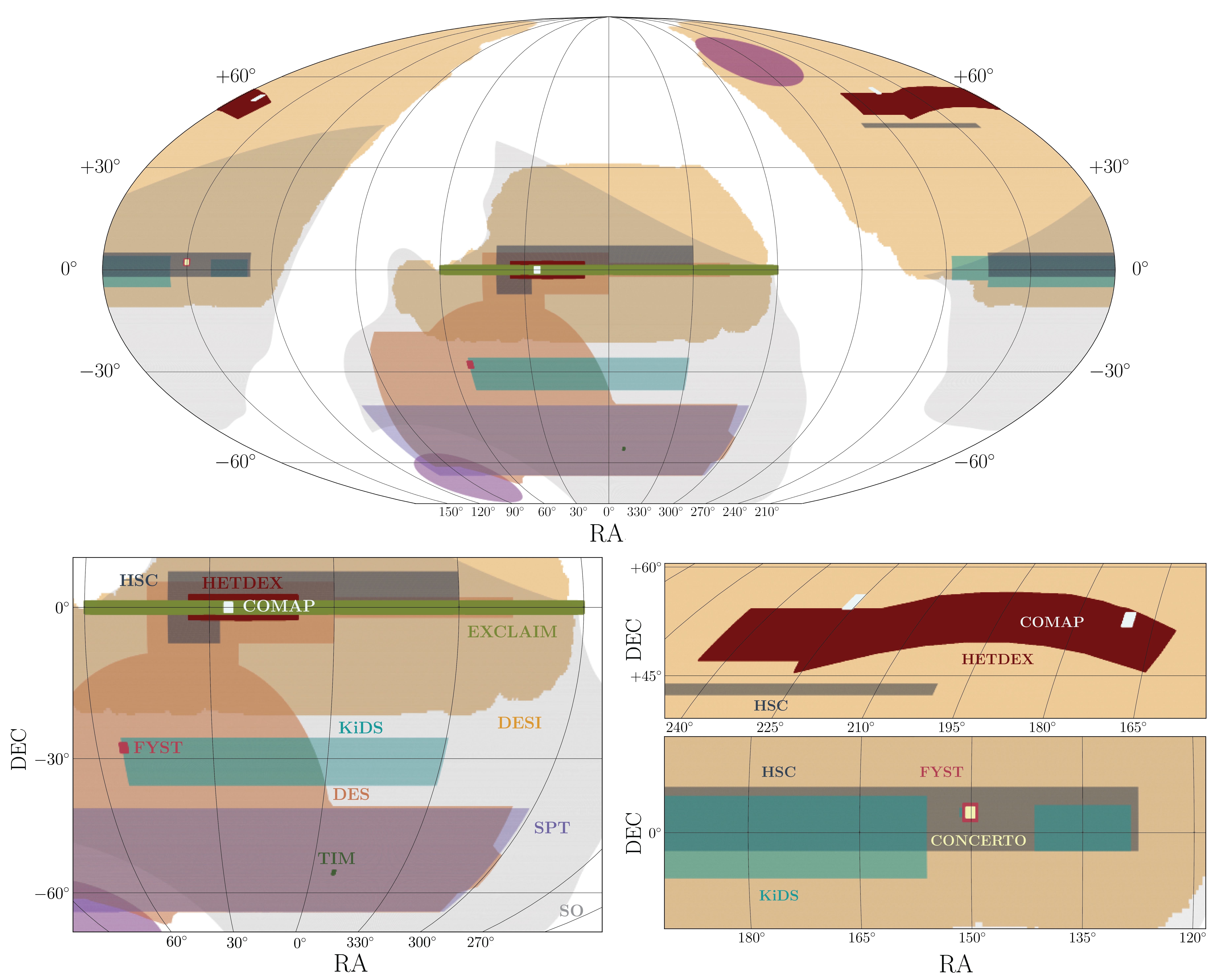
Figure 9: Mollweide projection in equatorial coordinates of the observing fields of a selection of current and forthcoming LIM surveys, galaxy surveys (HSC, KiDS, DES and DESI), and CMB experiments (SPT and SO). Bottom panels show zoom-in regions with LIM surveys. The purple circular regions in the top panel correspond to SPHEREx deep fields (overlapping with Euclid deep fields). We do not show mmIME and COPSS due to their small footprints, nor SPT-SLIM and TIME, since they have not finalized their observing fields yet (SPT-SLIM will observe within the SPT field), nor COSMOS and CDFS fields as they coincide with FYST fields and have similar areas.

6.1 Galaxy surveys

Line-intensity fluctuations are statistically correlated with other tracers of the large-scale structure, such as the galaxy distribution measured with galaxy surveys. Referring to quantities related to the galaxy field with a subscript ‘g’, the linear cross-power spectrum of galaxy number counts and intensity fluctuations of a line $X$ is

$$P^{Xg}=\langle T_{X}b_{X}\rangle b_{g}F^{X}_{\rm RSD}F^{g}_{\rm RSD}P_{\rm m}+X_{\rm LT}\frac{\langle\rho_{L}^{X}\rangle_{g}}{n_{g}}\,,$$ (30)

where $b_{g}$ is the galaxy bias, $F^{g}_{\rm RSD}$ is defined using $b_{g}$, $\langle\rho_{L}^{X}\rangle_{g}$ is the mean luminosity-density of line $X$ sourced only from galaxies included in the galaxy catalog considered, $n_{g}$ is the number density of those galaxies, and we have assumed a Poissonian galaxy shot noise Wolz:2017rlw ; 2019MNRAS.490..260B ; 2021ApJ…915…33S . Note that halo exclusion and clustering may cause galaxy shot noise to deviate from being Poissonian, changing its amplitude and even inducing a small scale dependence Ginzburg:2017mgf ; Schmittfull:2018yuk . Since uncorrelated foregrounds and line interlopers come from a different volume than the galaxy survey, they are not correlated with the galaxy distribution and their contribution is left out of the cross correlation, as discussed in Sec. 5.4. Nonetheless, all components of the line-intensity map do contribute to the cross-correlation covariance, which can be computed adapting Eq. (18).

On the other hand, LIM-galaxy cross correlations can also benefit galaxy surveys. As galaxy surveys extend their reach to higher redshifts, spectroscopic surveys become harder and the redshift uncertainties in photometric and radio-continuum surveys become larger. Therefore, techniques like clustering-based redshifts Menard:2013aaa ; McQuinn:2013ib ; Rahman:2014lfa —which uses a dataset with known redshifts to cross-correlate two-dimensional slices along the line of sight with the unknown dataset in order to retrieve the redshift distribution of the latter—can be applied using the superior spectral resolution of LIM surveys to improve the redshift determination of photometric galaxy surveys, as has been demonstrated in the case of HI LIM Alonso:2017dgh ; Cunnington:2018zxg ; Modi:2021okf . This also enables tomographic analyses in radio-continuum surveys Kovetz:2016hgp ; Bernal:2018myq .

In addition, cross correlations with specific galaxy populations can be used to obtain information about the IGM and ISM properties of such galaxies. At small scales, the cross-power spectrum depends on the mean line-intensity from that population of galaxies, which can be connected to the line models discussed in Sec. 3.2. Ref. 2019MNRAS.490..260B cross-correlated quasar positions with CO LIM measurements to study the abundance and excitation state of molecular gas within galaxies hosting active galactic nuclei. This approach, complementary to stacking analyses, can be extended to any line or galaxy population.

Galaxy surveys also target gravitational weak lensing through cosmic shear and galaxy shapes. Cross correlating LIM with cosmic shear maps allows us to connect the intensity fluctuations with the actual matter density fluctuations Schaan:2018yeh ; Foreman:2018gnv ; Schaan:2021gzb . The lensing kernel can be considered using the following transfer function in Eq. (20):

$$\Delta_{\ell}^{\kappa}(k,z)=\frac{3H_{0}^{2}\Omega_{\rm m}}{2c^{2}}(1+z)\int\displaylimits_{z}^{\rm z_{\rm max}}{\rm d}z^{\prime}\frac{{\rm d}n_{g}}{{\rm d}z^{\prime}}\frac{\chi(z)\left(\chi(z^{\prime})-\chi(z)\right)}{\chi(z^{\prime})}\mathcal{T}(k)j_{\ell}(k\chi)\,,$$ (31)

where ${\rm d}n_{g}/{\rm d}z$ is the galaxy redshift distribution normalized to unity. Ref. Chung:2022lpr presents a systematic study of the prospects of cross correlating LIM and projected cosmic shear maps, finding that current pathfinder experiments are expected to yield a marginally significant cross correlation with a survey like LSST, but future stage-3 experiments conceivably ready by the end of LSST will yield a high significance detection.

Degeneracies between LIM astrophysical dependence and intrinsic alignments may weaken the astrophysical constraints from LIM-shear analyses, but they will strongly constrain integrated quantities like the cosmic density of molecular hydrogen or the star-formation rate. Pushing LIM-shear studies to smaller scales will shed light on the baryonic feedback on matter overdensities. Furthermore, LIM-shear correlations provide additional information to constrain radiative decays of dark matter Shirasaki:2021yrp .

Potential improvements of this program include the use of tomographic cosmic shear, which is already available for shear auto-correlations and cross correlations with galaxy positions. However, using tomographic binning enhances the covariance due to shot noise, shape noise and the contribution from lines with null correlation with the cosmic shear bin. Finally, standard 3x2 analyses (galaxy clustering, galaxy clustering cross shear, and shear correlations) Heymans:2020gsg ; DES:2021wwk could be extended to 6x2 analyses (galaxy clustering, galaxy clustering cross shear, galaxy clustering cross LIM, shear, shear cross LIM, and LIM correlations).

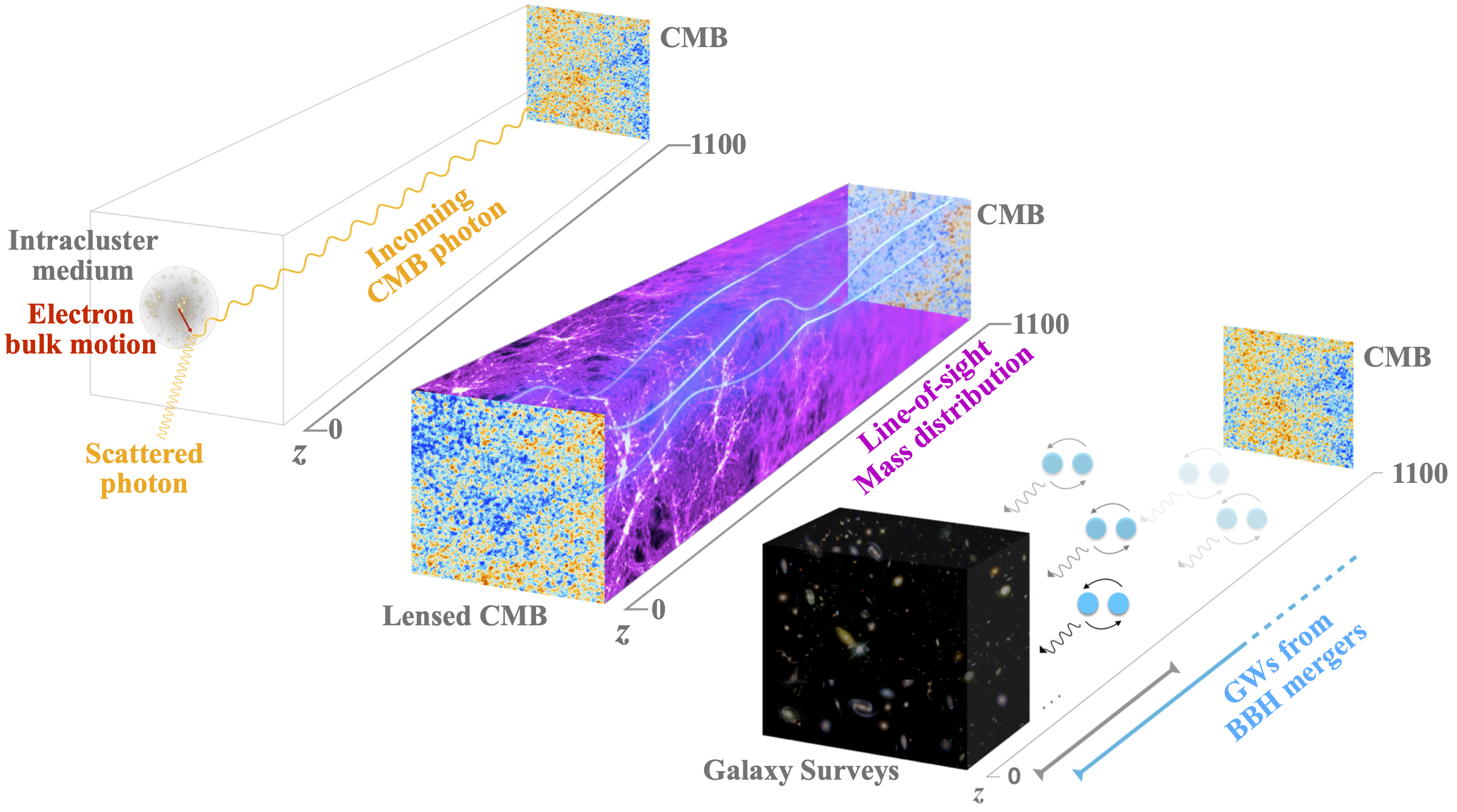
Figure 10: LIM can be cross correlated with other tracers of the line-of-sight mass distribution, including CMB secondaries such as the kinetic Sunyaev-Zel’dovich effect or weak gravitational lensing and transients like gravitational waves from binary black hole mergers.

6.2 CMB Secondary Anisotropies

CMB photons are exposed to the effects of cosmological structures that they encounter along their path as they travel from the last scattering surface to us. These interactions inflict further perturbations in their temperature and polarization, known as secondary anisotropies Aghanim:2007bt , including gravitational effects such as lensing Lewis:2006fu , integrated Sachs-Wolfe effect 1967ApJ…147…73S ; Rees:1968zza , and moving lens effects 1983Natur.302..315B , as well as photon-electron scattering described by different flavors of the Sunyaev-Zel’dovich (SZ) effect Zeldovich:1969ff ; Sunyaev:1970er ; Sunyaev:1972eq ; Sazonov:1999zp . Figure 10 illustrates some of these processes (as well as the overlap with transients, discussed later).

These secondary anisotropies can be detected in the CMB power spectrum, but are better isolated from the primary anisotropies in cross-correlation analyses with other tracers of large-scale structure. This allows for tomographic analyses instead of being limited to the integrated effect alone in CMB-only studies. This approach has been applied using galaxy surveys White:2021yvw ; DES:2018nlb ; Krolewski:2021znk ; Hotinli:2018yyc ; AtacamaCosmologyTelescope:2020wtv ; here we motivate the use of LIM in this context.

First, LIM-CMB cross correlations enable the extension of CMB secondary anisotropies tomography to higher redshifts. This is motivated by the wide support of some CMB secondary kernels in redshift, which goes beyond the current reach of galaxy surveys. LIM can also be used to remove the contribution from secondary anisotropies in CMB observations. The main contaminant is gravitational lensing, but its effect can be partially reversed internally or using external observations Smith:2010gu ; Carron:2017vfg , which improves cosmological parameter inference SPTpol:2020rqg ; BaleatoLizancos:2020mic ; Hotinli:2021umk . The CIB Sherwin:2015baa ; Larsen:2016wpa and especially LIM Karkare:2019qla can be used to improve this procedure. Alternatively, in the same way that CMB lensing can be used to improve the modeling of the CIB McCarthy:2020qjf , it may be possible to improve the modeling of the line emission. Furthermore, LIM properties provide access to intrinsically different information, as is the case of probing reionization with the cross correlation of high-redshift HI and SZ maps Ma:2017gey ; Li:2018izh ; LaPlante:2020nxx .

The late-time kinematic-SZ (kSZ) effect, detected both in the CMB temperature power spectrum George:2014oba and in cross correlation with galaxy surveys Hand:2012ui ; Planck:2015ywj ; DES:2016umt ; DeBernardis:2016pdv ; AtacamaCosmologyTelescope:2020wtv , can be used to reconstruct the matter velocity field at large scales. This reconstruction can be performed as a function of redshift by cross correlating kSZ maps with large-scale structure tracers Ho:2009iw ; Shao:2010md ; Smith:2018bpn . Ref. Sato-Polito:2022fkd presented a study of the potential to measure late-time kSZ tomography using LIM instead of galaxy surveys, with the [CII] emission line as an example. While a detection is beyond reach for the initial design of FYST, an upgraded design with higher sensitivity can achieve a $\sim 3\sigma$ detection in cross correlation with Simons Observatory at $z\sim 3.7$, with substantial improvements for third-generation LIM surveys, yielding up to $\sim 10^{2}\!-\!10^{3}$ detection significance.

The main limitation of CMB and LIM cross correlations is related to the contamination from continuum foregrounds. CMB secondary anisotropies are sensitive to quantities integrated along the line of sight, since they affect CMB photons as they propagate, which means that most of the information in their cross-correlation with large-scale structure tracers is contained in the long-wavelength line-of-sight components. As discussed in Sec. 5.4, these are the most affected by continuum foregrounds, which has been shown to limit the potential of reionization kSZ-HI cross-correlations LaPlante:2020nxx . This limitation also applies, to a lesser degree, to other cross-correlations discussed in this section. However, using high-order statistics or forward modelling Modi:2019hnu may retrieve some of the information.

6.3 Transient Catalogs

The recent discovery of gravitational-waves (GWs) from mergers of binary black holes and neutron stars has kick-started, together with neutrino observations, the era of multi-messenger astronomy. Over the past few years, the LIGO-VIRGO-KAGRA collaboration KAGRA:2013rdx has detected almost $100$ merger events in three observing runs. With planned improvements towards the next observing runs and the advent of next-generation observatories such as Cosmic Explorer LIGOScientific:2016wof and the Einstein Telescope Maggiore:2019uih , future GW catalogs are expected to amount to tens of thousands of events or more. As these mergers are detectable to high redshifts, GWs are destined to become a useful tracer of large-scale structure Libanore:2020fim .

Several other classes of astrophysical transients are within sight of becoming useful standalone tracers of large-scale structure at high-redshifts. These include gamma-ray bursts, supernovae, tidal disruption events and fast radio bursts (FRBs). Current catalogs of all these types of transients contain between dozens to thousand of events, but with ongoing and upcoming experimental programs we can expect at least a ten-fold increase in number over a ten-year timescale. For FRBs in particular, due to their extremely high rate Fialkov:2017qoz , we may expect a few orders of magnitude more events in future catalogs from CHIME CHIMEFRB:2021srp and other instruments.

One of the main drawbacks of transient-event catalogs such as GWs and FRBs is their poor redshift determination. A promising method to curb this limitation is clustering-based redshift estimation, mentioned above. Here LIM has potential for dramatic payoff, as its redshift information is by definition controllable via the observation frequency and its two-dimensional clustering can be extracted up to very high redshifts (see Fig. 2). Reconstructed redshift distributions will allow tomography, which enables several cosmological applications. For example, it can be used to greatly improve parameter estimation Kovetz:2016hgp , to constrain the expansion history of the Universe (when comparing redshifts to the luminosity distance or dispersion measure for GWs or FRBs, respectively) Scelfo:2021fqe ; Mukherjee:2021bmw , to measure the CMB optical depth to reionization Fialkov:2016fjb , to break the kinetic Sunyaev-Zel’dovich effect optical depth degeneracy Madhavacheril:2019buy and to constrain the gravitational-slip in modified gravity theories Abadi:2021ysz , to name a few.

Moreover, as both compact binary mergers and FRBs are expected to be related to properties of the stellar population, such as the star-formation rate and stellar mass in the host galaxy Artale:2019tfl , the metallicity distribution Dvorkin:2016wac , etc., there is promising complementarity between LIM and these transients. Their cross-correlation can help distinguish between GW progenitors Raccanelli:2016cud , constrain the origins of FRBs Zhang:2020ass , infer the delay-time distribution between binary formation and merger Safarzadeh:2019pis , and much more.

7 Conclusions

Here concludes our short review of the theory of LIM. After describing the basic idea behind LIM and summarizing the current experimental landscape, we introduced the primary emission lines targeted by these experiments, from the rotational CO transitions in the sub-mm, through the series of fine-structure lines such as [CII] in the infrared to hydrogen lines including H$\alpha$ and Ly$\alpha$ observed in the optical and UV, and discussed different approaches to modeling their luminosity functions. We then surveyed the prospects to use LIM to advance our understanding of major topics in astrophysics and cosmology, from star-formation history, the properties of the ISM and the process of reionization, to the search for dark matter and light relics and the study of cosmic inflation and dark energy. The heart of the review was dedicated to carefully laying out the modern formalism to describe the statistics of line-intensity maps, including the power spectrum and voxel-intensity distribution, with special attention to observational effects and cross-correlation. We also discussed the problem of interloper foregrounds which uniquely plagues this type of observation. Finally, we devoted a separate chapter to cross-correlation opportunities between LIM and other observables, from galaxy surveys to CMB secondary anisotropies to astrophysical transients.

We hope that this review successfully demonstrates the bright outlook for LIM as a burgeoning observable in high-redshift astrophysics and cosmology, that it provides a useful self-contained description of the theoretical backbone of the field for experts and newcomers alike, and that it affords the necessary tools for novices to pick up the gauntlet and join the effort to make LIM science a prosperous reality. In this spirit, we accompany its release with an updated online version of the lim package, and provide a few tutorial Jupyter notebooks that can be used to reproduce the main figures above.

- (1) C. J. Hogan and M. J. Rees, “Spectral appearance of non-uniform gas at high z.,” Mon. Not. R. Astron. Soc. 188 (Sept., 1979) 791–798.
- (2) M. Suginohara, T. Suginohara, and D. N. Spergel, “Detecting Z 10 objects through carbon, nitrogen and oxygen emission lines,” Astrophys. J. 512 (1999) 547, arXiv:astro-ph/9803236.
- (3) T.-C. Chang, U.-L. Pen, J. B. Peterson, and P. McDonald, “Baryon Acoustic Oscillation Intensity Mapping as a Test of Dark Energy,” Phys. Rev. Lett. 100 (2008) 091303, arXiv:0709.3672 [astro-ph].
- (4) E. Visbal and A. Loeb, “Measuring the 3D Clustering of Undetected Galaxies Through Cross Correlation of their Cumulative Flux Fluctuations from Multiple Spectral Lines,” JCAP 11 (2010) 016, arXiv:1008.3178.
- (5) E. Visbal, H. Trac, and A. Loeb, “Demonstrating the Feasibility of Line Intensity Mapping Using Mock Data of Galaxy Clustering from Simulations,” JCAP 08 (2011) 010, arXiv:1104.4809.
- (6) Y. Gong, A. Cooray, M. B. Silva, M. G. Santos, and P. Lubin, “Probing Reionization with Intensity Mapping of Molecular and Fine Structure Lines,” Astrophys. J. Lett. 728 (2011) L46, arXiv:1101.2892.
- (7) C. L. Carilli, “Intensity mapping of molecular gas during cosmic reionization,” Astrophys. J. Lett. 730 (2011) L30, arXiv:1102.0745.
- (8) J. Fonseca, M. Silva, M. G. Santos, and A. Cooray, “Cosmology with intensity mapping techniques using atomic and molecular lines,” Mon. Not. Roy. Astron. Soc. 464 no. 2, (2017) 1948–1965, arXiv:1607.05288.
- (9) E. D. Kovetz et al., “Line-Intensity Mapping: 2017 Status Report,” arXiv:1709.09066.
- (10) S. Furlanetto, S. P. Oh, and F. Briggs, “Cosmology at Low Frequencies: The 21 cm Transition and the High-Redshift Universe,” Phys. Rept. 433 (2006) 181–301, arXiv:astro-ph/0608032.
- (11) M. F. Morales and J. S. B. Wyithe, “Reionization and Cosmology with 21 cm Fluctuations,” Ann. Rev. Astron. Astrophys. 48 (2010) 127–171, arXiv:0910.3010.
- (12) J. R. Pritchard and A. Loeb, “21-cm cosmology,” Rept. Prog. Phys. 75 (2012) 086901, arXiv:1109.6012.
- (13) A. Liu and J. R. Shaw, “Data Analysis for Precision 21 cm Cosmology,” Publ. Astron. Soc. Pac. 132 no. 1012, (2020) 062001, arXiv:1907.08211.
- (14) D. J. Schlegel et al., “Astro2020 APC White Paper: The MegaMapper: a z 2 Spectroscopic Instrument for the Study of Inflation and Dark Energy,” arXiv:1907.11171.
- (15) B. D. Uzgil, J. E. Aguirre, C. M. Bradford, and A. Lidz, “Measuring Galaxy Clustering and the Evolution of [CII] Mean Intensity with far-IR Line Intensity Mapping During 0.5 1.5,” Astrophys. J. 793 no. 2, (2014) 116, arXiv:1407.4860.
- (16) Y.-T. Cheng, R. de Putter, T.-C. Chang, and O. Dore, “Optimally Mapping Large-Scale Structures with Luminous Sources,” Astrophys. J. 877 no. 2, (2019) 86, arXiv:1809.06384.
- (17) E. Schaan and M. White, “Astrophysics & Cosmology from Line Intensity Mapping vs Galaxy Surveys,” JCAP 05 (2021) 067, arXiv:2103.01971.
- (18) G. Sato-Polito, N. Kokron, and J. L. Bernal, “A multi-tracer empirically-driven approach to line-intensity mapping lightcones,” arXiv:2212.08056 [astro-ph.CO].
- (19) J. Kamenetzky, N. Rangwala, J. Glenn, P. R. Maloney, and A. Conley, “LCO/LFIR Relations with CO Rotational Ladders of Galaxies Across the Herschel SPIRE Archive,” Astrophys. J. 829 no. 2, (Oct., 2016) 93, arXiv:1508.05102.
- (20) I. De Looze et al., “The applicability of far-infrared fine-structure lines as star formation rate tracers over wide ranges of metallicities and galaxy types,” Astron. Astrophys. 568 (2014) A62, arXiv:1402.4075.
- (21) V. Desjacques, D. Jeong, and F. Schmidt, “Large-Scale Galaxy Bias,” Phys. Rept. 733 (2018) 1–193, arXiv:1611.09787.
- (22) A. Moradinezhad Dizgah, F. Nikakhtar, G. K. Keating, and E. Castorina, “Precision tests of CO and [CII] power spectra models against simulated intensity maps,” JCAP 02 no. 02, (2022) 026, arXiv:2111.03717.
- (23) L. J. Kewley, D. C. Nicholls, and R. S. Sutherland, “Understanding Galaxy Evolution Through Emission Lines,” Annu. Rev. Astron. Astrophys. 57 (Aug., 2019) 511–570, arXiv:1910.09730.
- (24) G. K. Keating et al., “First Results from COPSS: The CO Power Spectrum Survey,” Astrophys. J. 814 no. 2, (2015) 140, arXiv:1510.06744.
- (25) G. K. Keating, D. P. Marrone, G. C. Bower, E. Leitch, J. E. Carlstrom, and D. R. DeBoer, “COPSS II: The molecular gas content of ten million cubic megaparsecs at redshift z 3,” Astrophys. J. 830 no. 1, (2016) 34, arXiv:1605.03971.
- (26) G. K. Keating, D. P. Marrone, G. C. Bower, and R. P. Keenan, “An Intensity Mapping Detection of Aggregate CO Line Emission at 3 mm,” Astrophys. J. 901 no. 2, (2020) 141, arXiv:2008.08087.
- (27) COMAP Collaboration, K. A. Cleary et al., “COMAP Early Science: I. Overview,” arXiv:2111.05927.
- (28) COMAP Collaboration, P. C. Breysse et al., “COMAP Early Science: VII. Prospects for CO Intensity Mapping at Reionization,” arXiv:2111.05933.
- (29) CCAT-Prime Collaboration, M. Aravena et al., “CCAT-prime Collaboration: Science Goals and Forecasts with Prime-Cam on the Fred Young Submillimeter Telescope,” arXiv:2107.10364.
- (30) K. S. Karkare et al., “SPT-SLIM: A Line Intensity Mapping Pathfinder for the South Pole Telescope,” in 19th International Workshop on Low Temperature Detectors. 11, 2021. arXiv:2111.04631.
- (31) Concerto Collaboration, P. Ade, M. Aravena, E. Barria, A. Beelen, A. Benoit, et al., “A wide field-of-view low-resolution spectrometer at APEX: Instrument design and scientific forecast,” Astron. Astrophys. 642 (Oct., 2020) A60.
- (32) A. T. Crites, J. J. Bock, C. M. Bradford, T. C. Chang, A. R. Cooray, L. Duband, et al., “The TIME-Pilot intensity mapping experiment,” in Millimeter, Submillimeter, and Far-Infrared Detectors and Instrumentation for Astronomy VII, W. S. Holland and J. Zmuidzinas, eds., vol. 9153 of Society of Photo-Optical Instrumentation Engineers (SPIE) Conference Series, p. 91531W. Aug., 2014.
- (33) G. Sun et al., “Probing Cosmic Reionization and Molecular Gas Growth with TIME,” Astrophys. J. 915 no. 1, (2021) 33, arXiv:2012.09160.
- (34) E. R. Switzer, E. M. Barrentine, G. Cataldo, T. Essinger-Hileman, P. A. R. Ade, C. J. Anderson, et al., “Experiment for cryogenic large-aperture intensity mapping: instrument design,” Journal of Astronomical Telescopes, Instruments, and Systems 7 (Oct., 2021) 044004.
- (35) J. Vieira, J. Aguirre, C. M. Bradford, J. Filippini, C. Groppi, D. Marrone, et al., “The Terahertz Intensity Mapper (TIM): a Next-Generation Experiment for Galaxy Evolution Studies,” arXiv e-prints (Sept., 2020) arXiv:2009.14340, arXiv:2009.14340.
- (36) G. J. Hill et al., “The Hobby-Eberly Telescope Dark Energy Experiment (HETDEX): Description and Early Pilot Survey Results,” ASP Conf. Ser. 399 (2008) 115–118, arXiv:0806.0183 [astro-ph].
- (37) K. Gebhardt et al., “The Hobby–Eberly Telescope Dark Energy Experiment (HETDEX) Survey Design, Reductions, and Detections*,” Astrophys. J. 923 no. 2, (2021) 217, arXiv:2110.04298.
- (38) O. Doré, J. Bock, M. Ashby, P. Capak, A. Cooray, R. de Putter, et al., “Cosmology with the SPHEREX All-Sky Spectral Survey,” arXiv e-prints (Dec., 2014) arXiv:1412.4872, arXiv:1412.4872.
- (39) P. D. Klaassen, T. K. Mroczkowski, C. Cicone, E. Hatziminaoglou, S. Sartori, C. De Breuck, et al., “The Atacama Large Aperture Submillimeter Telescope (AtLAST),” in Society of Photo-Optical Instrumentation Engineers (SPIE) Conference Series, vol. 11445. Dec., 2020. arXiv:2011.07974.
- (40) A. Cooray et al., “Cosmic Dawn Intensity Mapper,” arXiv:1602.05178.
- (41) A. Cooray, T.-C. Chang, S. Unwin, M. Zemcov, A. Coffey, P. Morrissey, et al., “Cosmic Dawn Intensity Mapper,” in Bulletin of the American Astronomical Society, vol. 51, p. 23. Sept., 2019. arXiv:1903.03144.
- (42) M. B. Silva, E. D. Kovetz, G. K. Keating, A. Moradinezhad Dizgah, M. Bethermin, P. C. Breysse, et al., “Mapping large-scale-structure evolution over cosmic times,” Exper. Astron. 51 no. 3, (2021) 1593–1622, arXiv:1908.07533.
- (43) J. Delabrouille et al., “Microwave spectro-polarimetry of matter and radiation across space and time,” Exper. Astron. 51 no. 3, (2021) 1471–1514, arXiv:1909.01591.
- (44) E. D. Kovetz et al., “Astrophysics and Cosmology with Line-Intensity Mapping,” Bull. Am. Astron. Soc. 51 no. 3, (2020) 101, arXiv:1903.04496.
- (45) R. C. Kennicutt, Jr. and N. J. Evans, II, “Star Formation in the Milky Way and Nearby Galaxies,” Ann. Rev. Astron. Astrophys. 50 (2012) 531–608, arXiv:1204.3552.
- (46) P. Madau and M. Dickinson, “Cosmic Star Formation History,” Ann. Rev. Astron. Astrophys. 52 (2014) 415–486, arXiv:1403.0007.
- (47) S. Heinis et al., “HerMES: dust attenuation and star formation activity in UV-selected samples from z~4 to z~1.5,” Mon. Not. Roy. Astron. Soc. 437 no. 2, (2014) 1268–1283, arXiv:1310.3227.
- (48) R. J. Bouwens, M. Aravena, R. Decarli, F. Walter, E. da Cunha, I. Labbé, et al., “ALMA Spectroscopic Survey in the Hubble Ultra Deep Field: The Infrared Excess of UV-Selected z = 2-10 Galaxies as a Function of UV-Continuum Slope and Stellar Mass,” Astrophys. J. 833 no. 1, (Dec., 2016) 72, arXiv:1606.05280.
- (49) R. Bouwens, J. González-López, M. Aravena, R. Decarli, M. Novak, M. Stefanon, et al., “The ALMA Spectroscopic Survey Large Program: The Infrared Excess of z = 1.5-10 UV-selected Galaxies and the Implied High-redshift Star Formation History,” Astrophys. J. 902 no. 2, (Oct., 2020) 112, arXiv:2009.10727.
- (50) T. L. Wilson and D. Elbaz, “Report by the ESA-ESO Working Group on The Herschel-ALMA Synergies,” arXiv:astro-ph/0609311.
- (51) J. Chevallard and S. Charlot, “Modelling and interpreting spectral energy distributions of galaxies with BEAGLE,” Mon. Not. R. Astron. Soc. 462 no. 2, (Oct., 2016) 1415–1443, arXiv:1603.03037.
- (52) Y. Harikane, M. Ouchi, T. Shibuya, T. Kojima, H. Zhang, R. Itoh, et al., “SILVERRUSH. V. Census of Ly, [O III] 5007, H, and [C II] 158 m Line Emission with 1000 LAEs at z = 4.9-7.0 Revealed with Subaru/HSC,” Astrophys. J. 859 no. 2, (June, 2018) 84, arXiv:1711.03735.
- (53) P. M. Solomon, A. R. Rivolo, J. Barrett, and A. Yahil, “Mass, luminosity, and line width relations of Galactic molecular clouds,” Astrophys. J. 319 (1987) 730–741.
- (54) T. M. Dame, D. Hartmann, and P. Thaddeus, “The Milky Way in molecular clouds: A New complete co survey,” Astrophys. J. 547 (2001) 792–813, arXiv:astro-ph/0009217.
- (55) F. Walter, F. Bertoldi, C. Carilli, P. Cox, K. Y. Lo, R. Neri, et al., “Molecular gas in the host galaxy of a quasar at redshift z=6.42,” Nature 424 (2003) 406–408, arXiv:astro-ph/0307410.
- (56) R. J. Ivison, P. P. Papadopoulos, I. Smail, T. R. Greve, A. P. Thomson, E. M. Xilouris, and S. C. Chapman, “Tracing the molecular gas in distant submillimetre galaxies via CO(1-0) imaging with the EVLA,” Mon. Not. Roy. Astron. Soc. 412 (2011) 1913, arXiv:1009.0749.
- (57) A. Saintonge, G. Kauffmann, C. Kramer, L. J. Tacconi, C. Buchbender, B. Catinella, et al., “COLD GASS, an IRAM legacy survey of molecular gas in massive galaxies - I. Relations between H2, H I, stellar content and structural properties,” Mon. Not. R. Astron. Soc. 415 no. 1, (July, 2011) 32–60, arXiv:1103.1642.
- (58) C. Carilli and F. Walter, “Cool Gas in High Redshift Galaxies,” Ann. Rev. Astron. Astrophys. 51 (2013) 105–161, arXiv:1301.0371.
- (59) D. Narayanan, M. R. Krumholz, E. C. Ostriker, and L. Hernquist, “A General Model for the CO-H2 Conversion Factor in Galaxies with Applications to the Star Formation Law,” Mon. Not. Roy. Astron. Soc. 421 (2012) 3127, arXiv:1110.3791.
- (60) A. D. Bolatto, M. Wolfire, and A. K. Leroy, “The CO-to- Conversion Factor,” Ann. Rev. Astron. Astrophys. 51 (2013) 207–268, arXiv:1301.3498.
- (61) M. Heyer and T. M. Dame, “Molecular Clouds in the Milky Way,” Annu. Rev. Astron. Astrophys. 53 (Aug., 2015) 583–629.
- (62) R. L. Dickman, R. L. Snell, and F. P. Schloerb, “Carbon Monoxide as an Extragalactic Mass Tracer,” Astrophys. J. 309 (Oct., 1986) 326.
- (63) L. J. Tacconi, R. Genzel, and A. Sternberg, “The Evolution of the Star-Forming Interstellar Medium Across Cosmic Time,” Ann. Rev. Astron. Astrophys. 58 (2020) 157–203, arXiv:2003.06245.
- (64) H. S. Liszt and J. Pety, “Imaging diffuse clouds: Bright and dark gas mapped in CO,” Astron. Astrophys. 541 (2012) A58, arXiv:1202.6523.
- (65) R. Genzel et al., “The metallicity dependence of the CO \rightarrow H_2 conversion factor in z1 star forming galaxies,” Astrophys. J. 746 (2012) 69, arXiv:1106.2098.
- (66) G. Popping, R. S. Somerville, and S. C. Trager, “Evolution of the atomic and molecular gas content of galaxies,” Mon. Not. Roy. Astron. Soc. 442 no. 3, (2014) 2398–2418, arXiv:1308.6764.
- (67) R. L. Sanders, A. E. Shapley, T. Jones, I. Shivaei, G. Popping, N. A. Reddy, et al., “CO Emission, Molecular Gas, and Metallicity in Main-Sequence Star-Forming Galaxies at ,” arXiv e-prints (Apr., 2022) arXiv:2204.06937, arXiv:2204.06937.
- (68) M. R. Krumholz, A. K. Leroy, and C. F. McKee, “What Phase of the Interstellar Medium Correlates with the Star Formation Rate?,” Astrophys. J. 731 (2011) 25, arXiv:1101.1296.
- (69) D. Downes and P. M. Solomon, “Rotating nuclear rings and extreme starbursts in ultraluminous galaxies,” Astrophys. J. 507 (1998) 615, arXiv:astro-ph/9806377.
- (70) D. Narayanan, C. K. Walker, and C. E. Groppi, “Warm-dense molecular gas in the ISM of starbursts, LIRGs and ULIRGs,” Astrophys. J. 630 (2005) 269–279, arXiv:astro-ph/0504412. [Erratum: Astrophys.J. 642, 616 (2006), Erratum: Astrophys.J. 721, 921 (2010)].
- (71) P. P. Papadopoulos, P. van der Werf, E. M. Xilouris, K. G. Isaak, Y. Gao, and S. Muehle, “The molecular gas in Luminous Infrared Galaxies I: CO lines, extreme physical conditions, and their drivers,” Mon. Not. Roy. Astron. Soc. 426 (2012) 2601, arXiv:1109.4176.
- (72) T. G. Bisbas, P. P. Papadopoulos, and S. Viti, “Effective Destruction of CO by Cosmic Rays: Implications for Tracing H2 Gas in the Universe,” Astrophys. J. 803 no. 1, (Apr., 2015) 37, arXiv:1502.04198.
- (73) P. C. Breysse, S. Yang, R. S. Somerville, A. R. Pullen, G. Popping, and A. S. Maniyar, “On Estimating the Cosmic Molecular Gas Density from CO Line Intensity Mapping Observations,” Astrophys. J. 929 no. 1, (2022) 30, arXiv:2106.14904.
- (74) P. M. Solomon and P. A. Vanden Bout, “Molecular gas at high redshift,” Ann. Rev. Astron. Astrophys. 43 (2005) 677–725, arXiv:astro-ph/0508481.
- (75) P. C. Breysse, S. Foreman, L. C. Keating, J. Meyers, and N. Murray, “Mapping the Universe in hydrogen deuteride,” Phys. Rev. D 105 no. 8, (2022) 083009, arXiv:2104.06422.
- (76) P. C. Breysse and M. Rahman, “Feeding cosmic star formation: Exploring high-redshift molecular gas with CO intensity mapping,” Mon. Not. Roy. Astron. Soc. 468 no. 1, (2017) 741–750, arXiv:1606.07820.
- (77) F. P. Israel, M. J. F. Rosenberg, and P. van der Werf, “Neutral carbon and CO in 76 (U)LIRGs and starburst galaxy centers. A method to determine molecular gas properties in luminous galaxies,” Astron. Astrophys. 578 (June, 2015) A95, arXiv:1504.08005.
- (78) Q. Jiao, Y. Zhao, M. Zhu, N. Lu, Y. Gao, and Z.-Y. Zhang, “Neutral Carbon Emission in Luminous Infrared Galaxies: The [C i] Lines as Total Molecular Gas Tracers,” Astrophys. J. Lett. 840 no. 2, (2017) L18, arXiv:1704.07780.
- (79) F. Valentino, G. E. Magdis, E. Daddi, D. Liu, M. Aravena, F. Bournaud, et al., “A Survey of Atomic Carbon [C I] in High-redshift Main-sequence Galaxies,” Astrophys. J. 869 no. 1, (Dec., 2018) 27, arXiv:1810.11029.
- (80) N. P. H. Nesvadba, R. Cañameras, R. Kneissl, S. Koenig, C. Yang, E. Le Floc’h, et al., “Planck’s Dusty GEMS. VII. Atomic carbon and molecular gas in dusty starburst galaxies at z = 2 to 4,” Astron. Astrophys. 624 (Apr., 2019) A23, arXiv:1812.04653.
- (81) D. T. Chung, “Cross-correlations between mm-wave line-intensity mapping and weak lensing surveys: preliminary consideration of long-term prospects,” arXiv:2203.12581.
- (82) M. Bethermin et al., “CONCERTO: High-fidelity simulation of millimeter line emissions of galaxies and [CII] intensity mapping,” arXiv:2204.12827.
- (83) P. C. Breysse, E. D. Kovetz, and M. Kamionkowski, “Masking line foregrounds in intensity mapping surveys,” Mon. Not. Roy. Astron. Soc. 452 no. 4, (2015) 3408–3418, arXiv:1503.05202.
- (84) D. T. Chung, T. Y. Li, M. P. Viero, S. E. Church, and R. H. Wechsler, “On estimation of contamination from hydrogen cyanide in carbon monoxide line intensity mapping,” Astrophys. J. 846 no. 1, (2017) 60, arXiv:1706.03005.
- (85) G. J. Stacey, S. Hailey-Dunsheath, C. Ferkinhoff, T. Nikola, S. C. Parshley, D. J. Benford, et al., “A 158 Micron [CII] Line Survey of Galaxies at z ~ 1 to 2: An Indicator of Star Formation in the Early Universe,” Astrophys. J. 724 (2010) 957–974, arXiv:1009.4216.
- (86) A. G. G. M. Tielens and D. Hollenbach, “Photodissociation regions. I - Basic model. II - A Model for the Orion photodissociation region,” Astrophys. J. 291 (1985) 722–754.
- (87) G. J. Stacey, N. Geis, R. Genzel, J. B. Lugten, A. Poglitsch, A. Sternberg, and C. H. Townes, “The 158 micron forbidden C II line: A measure of global star formation activity in galaxies,” Astrophys. J. 373 (1991) 423–444.
- (88) M. G. Wolfire, L. Vallini, and M. Chevance, “Photodissociation and X-Ray Dominated Regions,” arXiv:2202.05867.
- (89) A. Zanella, E. Daddi, G. Magdis, T. Diaz Santos, D. Cormier, D. Liu, et al., “The [C II] emission as a molecular gas mass tracer in galaxies at low and high redshifts,” Mon. Not. R. Astron. Soc. 481 no. 2, (Dec., 2018) 1976–1999, arXiv:1808.10331.
- (90) D. Vizgan, T. R. Greve, K. P. Olsen, A. Zanella, D. Narayanan, R. Davè, et al., “Tracing Molecular Gas in z 6 Galaxies with [C],” arXiv e-prints (Mar., 2022) arXiv:2203.05316, arXiv:2203.05316.
- (91) T. M. Hughes, K. Foyle, M. R. P. Schirm, T. J. Parkin, I. De Looze, C. D. Wilson, et al., “Insights into gas heating and cooling in the disc of NGC 891 from Herschel far-infrared spectroscopy,” Astron. Astrophys. 575 (Mar., 2015) A17, arXiv:1410.6156.
- (92) K. V. Croxall, J. D. Smith, E. Pellegrini, B. Groves, A. Bolatto, R. Herrera-Camus, et al., “The Origins of [C II] Emission in Local Star-forming Galaxies,” Astrophys. J. 845 no. 2, (Aug., 2017) 96, arXiv:1707.04435.
- (93) D. Cormier, N. P. Abel, S. Hony, V. Lebouteiller, S. C. Madden, F. L. Polles, et al., “The Herschel Dwarf Galaxy Survey. II. Physical conditions, origin of [C II] emission, and porosity of the multiphase low-metallicity ISM,” Astron. Astrophys. 626 (June, 2019) A23, arXiv:1904.08434.
- (94) R. C. Young Owl, M. M. Meixner, D. Fong, M. R. Haas, A. L. Rudolph, and A. G. G. M. Tielens, “Testing Models of Low-Excitation Photodissociation Regions with Far-Infrared Observations of Reflection Nebulae,” Astrophys. J. 578 (2002) 885–896.
- (95) E. L. O. Bakes and A. G. G. M. Tielens, “The photoelectric heating mechanism for very small graphitic grains and polycyclic aromatic hydrocarbons,” Astrophys. J. 427 (1994) 822–838.
- (96) J. A. Muñoz and S. P. Oh, “High-temperature saturation can produce the [C II] deficit in LIRGs and ULIRGs,” Mon. Not. R. Astron. Soc. 463 no. 2, (Dec., 2016) 2085–2091, arXiv:1510.00397.
- (97) M. Rybak, G. Calistro Rivera, J. A. Hodge, I. Smail, F. Walter, P. van der Werf, et al., “Strong Far-ultraviolet Fields Drive the [C II]/Far-infrared Deficit in z 3 Dusty, Star-forming Galaxies,” Astrophys. J. 876 no. 2, (May, 2019) 112, arXiv:1901.10027.
- (98) I. De Looze, M. Baes, G. J. Bendo, L. Cortese, and J. Fritz, “The reliability of [CII] as a star formation rate indicator,” Mon. Not. Roy. Astron. Soc. 416 (2011) 2712, arXiv:1106.1643.
- (99) R. Herrera-Camus et al., “[CII] 158 m Emission as a Star Formation Tracer,” Astrophys. J. 800 no. 1, (2015) 1, arXiv:1409.7123.
- (100) A. Ferrara, L. Vallini, A. Pallottini, S. Gallerani, S. Carniani, M. Kohandel, et al., “A physical model for [C II] line emission from galaxies,” Mon. Not. R. Astron. Soc. 489 no. 1, (Oct., 2019) 1–12, arXiv:1908.07536.
- (101) T. G. Bisbas, S. Walch, T. Naab, N. Lahén, R. Herrera-Camus, U. P. Steinwandel, et al., “The origin of the [CII]-deficit in a simulated dwarf galaxies starburst,” arXiv e-prints (May, 2022) arXiv:2205.08905, arXiv:2205.08905.
- (102) L. Vallini, S. Gallerani, A. Ferrara, A. Pallottini, and B. Yue, “On the [CII]-SFR Relation in High Redshift Galaxies,” Astrophys. J. 813 no. 1, (Nov., 2015) 36, arXiv:1507.00340.
- (103) K. Olsen, T. R. Greve, D. Narayanan, R. Thompson, R. Davé, L. Niebla Rios, and S. Stawinski, “SÍGAME Simulations of the [CII], [OI], and [OIII] Line Emission from Star-forming Galaxies at ,” Astrophys. J. 846 no. 2, (Sept., 2017) 105, arXiv:1708.04936.
- (104) G. Lagache, M. Cousin, and M. Chatzikos, “The [CII] 158 m line emission in high-redshift galaxies,” Astron. Astrophys. 609 (Jan., 2018) A130, arXiv:1711.00798.
- (105) U. Gorti and D. Hollenbach, “Photoevaporation of clumps in photodissociation regions,” Astrophys. J. 573 (2002) 215, arXiv:astro-ph/0204180.
- (106) D. Decataldo, A. Ferrara, A. Pallottini, S. Gallerani, and L. Vallini, “Molecular clumps photoevaporation in ionized regions,” Mon. Not. R. Astron. Soc. 471 no. 4, (Nov., 2017) 4476–4487, arXiv:1707.08574.
- (107) D. Decataldo, A. Pallottini, A. Ferrara, L. Vallini, and S. Gallerani, “Photoevaporation of Jeans-unstable molecular clumps,” Mon. Not. R. Astron. Soc. 487 no. 3, (Aug., 2019) 3377–3391, arXiv:1905.13230.
- (108) L. Vallini, A. Ferrara, A. Pallottini, and S. Gallerani, “Molecular cloud photoevaporation and far-infrared line emission,” Mon. Not. R. Astron. Soc. 467 no. 2, (May, 2017) 1300–1312, arXiv:1606.08464.
- (109) T. Díaz-Santos, L. Armus, V. Charmandaris, N. Lu, S. Stierwalt, G. Stacey, et al., “A Herschel/PACS Far-infrared Line Emission Survey of Local Luminous Infrared Galaxies,” Astrophys. J. 846 no. 1, (Sept., 2017) 32, arXiv:1705.04326.
- (110) D. Narayanan and M. R. Krumholz, “A physical model for the [C II]-FIR deficit in luminous galaxies,” Mon. Not. R. Astron. Soc. 467 no. 1, (May, 2017) 50–67, arXiv:1601.05803.
- (111) R. Herrera-Camus, E. Sturm, J. Graciá-Carpio, D. Lutz, A. Contursi, S. Veilleux, et al., “SHINING, A Survey of Far-infrared Lines in Nearby Galaxies. II. Line-deficit Models, AGN Impact, [C II]-SFR Scaling Relations, and Mass-Metallicity Relation in (U)LIRGs,” Astrophys. J. 861 no. 2, (July, 2018) 95, arXiv:1803.04422.
- (112) P. Serra, O. Doré, and G. Lagache, “Dissecting the high-z interstellar medium through intensity mapping cross-correlations,” Astrophys. J. 833 no. 2, (2016) 153, arXiv:1608.00585.
- (113) G. Sun, B. S. Hensley, T.-C. Chang, O. Doré, and P. Serra, “A Self-consistent Framework for Multiline Modeling in Line Intensity Mapping Experiments,” Astrophys. J. 887 no. 2, (Dec., 2019) 142, arXiv:1907.02999.
- (114) S. Yang and A. Lidz, “An analytic model for [O III] fine structure emission from high redshift galaxies,” Mon. Not. R. Astron. Soc. 499 no. 3, (Dec., 2020) 3417–3433, arXiv:2007.14439.
- (115) S. Yang, A. Lidz, and G. Popping, “The prospects for observing [O III] 52 micron emission from galaxies during the Epoch of Reionization,” Mon. Not. R. Astron. Soc. 504 no. 1, (June, 2021) 723–730, arXiv:2101.00662.
- (116) H. Padmanabhan, P. Breysse, A. Lidz, and E. R. Switzer, “Intensity mapping from the sky: synergizing the joint potential of [OIII] and [CII] surveys at reionization,” arXiv:2105.12148.
- (117) A. F. R. Padilla, L. Wang, F. F. S. van der Tak, and S. Trager, “Diagnosing the interstellar medium of galaxies with far-infrared emission lines II. [C II], [O I], [O III], [N II] and [N III] up to z=6,” arXiv:2205.11955.
- (118) N. Laporte et al., “The absence of [C ii] 158 m emission in spectroscopically confirmed galaxies at z 8,” Mon. Not. Roy. Astron. Soc. 487 no. 1, (2019) L81–L85, arXiv:1906.01937.
- (119) S. Carniani et al., “Missing [C II] emission from early galaxies,” Mon. Not. Roy. Astron. Soc. 499 no. 4, (2020) 5136–5150, arXiv:2006.09402.
- (120) P. F. Goldsmith, U. A. Yıldız, W. D. Langer, and J. L. Pineda, “Herschel Galactic Plane Survey of [NII] Fine Structure Emission,” Astrophys. J. 814 no. 2, (Dec., 2015) 133, arXiv:1510.05706.
- (121) R. Herrera-Camus, A. Bolatto, J. D. Smith, B. Draine, E. Pellegrini, M. Wolfire, et al., “The Ionized Gas in Nearby Galaxies as Traced by the [N II] 122 and 205 m Transitions,” Astrophys. J. 826 no. 2, (Aug., 2016) 175, arXiv:1605.03180.
- (122) M. Ouchi, Y. Ono, and T. Shibuya, “Observations of the Lyman- Universe,” Ann. Rev. Astron. Astrophys. 58 (2020) 617–659, arXiv:2012.07960.
- (123) M. R. Santos, “Probing reionization with Lyman-alpha emission lines,” Mon. Not. Roy. Astron. Soc. 349 (2004) 1137, arXiv:astro-ph/0308196.
- (124) P. Santini et al., “The evolution of the dust and gas content in galaxies,” Astron. Astrophys. 562 (2014) A30, arXiv:1311.3670.
- (125) C. C. Steidel, M. Bogosavljevic, A. E. Shapley, J. A. Kollmeier, N. A. Reddy, D. K. Erb, and M. Pettini, “Diffuse Lyman Alpha Emitting Halos: A Generic Property of High Redshift Star Forming Galaxies,” Astrophys. J. 736 (2011) 160, arXiv:1101.2204.
- (126) Z. Zheng, R. Cen, D. Weinberg, H. Trac, and J. Miralda-Escude, “Extended Lyman-Alpha Emission around Star-forming Galaxies,” Astrophys. J. 739 (2011) 62, arXiv:1010.3017.
- (127) A. Beane and A. Lidz, “Extracting bias using the cross-bispectrum: An EoR and 21 cm-[CII]-[CII] case study,” Astrophys. J. 867 no. 1, (2018) 26, arXiv:1806.02796.
- (128) K. Moriwaki, N. Yoshida, M. B. Eide, and B. Ciardi, “Cross-correlation between the 21-cm signal and [OIII] emitters during early cosmic reionization,” Mon. Not. Roy. Astron. Soc. 489 no. 2, (2019) 2471–2477, arXiv:1906.10863.
- (129) E. Sobacchi, A. Mesinger, and B. Greig, “Cross-correlation of the cosmic 21-cm signal and Lyman emitters during reionization,” Mon. Not. Roy. Astron. Soc. 459 no. 3, (2016) 2741–2750, arXiv:1602.04837.
- (130) M. B. Silva, S. Zaroubi, R. Kooistra, and A. Cooray, “Tomographic Intensity Mapping versus Galaxy Surveys: Observing the Universe in H-alpha emission with new generation instruments,” arXiv e-prints (Nov., 2017) arXiv:1711.09902, arXiv:1711.09902.
- (131) D. E. Osterbrock and G. J. Ferland, Astrophysics of gaseous nebulae and active galactic nuclei. 2006.
- (132) R. C. Kennicutt, Jr., “Star formation in galaxies along the Hubble sequence,” Ann. Rev. Astron. Astrophys. 36 (1998) 189–231, arXiv:astro-ph/9807187.
- (133) C. Ly, M. A. Malkan, N. Kashikawa, K. Shimasaku, M. Doi, T. Nagao, et al., “The Luminosity Function and Star Formation Rate between Redshifts of 0.07 and 1.47 for Narrow-band Emitters in the Subaru Deep Field,” Astrophys. J. 657 (2007) 738–759, arXiv:astro-ph/0610846.
- (134) S. Saito, S. de la Torre, O. Ilbert, C. Dubois, K. Yabe, and J. Coupon, “The Synthetic Emission Line COSMOS catalog: H and [OII] galaxy luminosity functions and counts at ,” Mon. Not. Roy. Astron. Soc. 494 no. 1, (2020) 199–217, arXiv:2003.06394.
- (135) E. Visbal, Z. Haiman, and G. L. Bryan, “Looking for Population III stars with He II line intensity mapping,” Mon. Not. Roy. Astron. Soc. 450 no. 3, (2015) 2506–2513, arXiv:1501.03177.
- (136) J. Parsons, L. Mas-Ribas, G. Sun, T.-C. Chang, M. O. Gonzalez, and R. H. Mebane, “Probing Population III IMFs with He II/H Intensity Mapping,” arXiv:2112.06407.
- (137) D. Schaerer, “On the Properties of massive population III stars and metal-free stellar populations,” Astron. Astrophys. 382 (2002) 28–42, arXiv:astro-ph/0110697.
- (138) Y. Gong, X. Chen, and A. Cooray, “Cosmological constraints from line intensity mapping with interlopers,” Astrophys. J. 894 no. 2, (2020) 152, arXiv:2001.10792.
- (139) L. Pozzetti, C. M. Hirata, J. E. Geach, A. Cimatti, C. Baugh, O. Cucciati, et al., “Modelling the number density of H emitters for future spectroscopic near-IR space missions,” Astron. Astrophys. 590 (2016) A3, arXiv:1603.01453.
- (140) J. A. Villa-Vélez, V. Buat, P. Theulé, M. Boquien, and D. Burgarella, “Fitting spectral energy distributions of FMOS-COSMOS emission-line galaxies at z 1.6: Star formation rates, dust attenuation, and [OIII]5007 emission-line luminosities,” Astron. Astrophys. 654 (2021) A153, arXiv:2108.13321.
- (141) A. Raichoor et al., “The SDSS-IV Extended Baryon Oscillation Spectroscopic Survey: final Emission Line Galaxy Target Selection,” Mon. Not. Roy. Astron. Soc. 471 no. 4, (2017) 3955–3973, arXiv:1704.00338.
- (142) A. Raichoor et al., “Preliminary Target Selection for the DESI Emission Line Galaxy (ELG) Sample,” Res. Notes AAS 4 no. 10, (2020) 180, arXiv:2010.11281.
- (143) R. Decarli, F. Walter, J. Gónzalez-López, M. Aravena, L. Boogaard, C. Carilli, et al., “The ALMA Spectroscopic Survey in the HUDF: CO Luminosity Functions and the Molecular Gas Content of Galaxies through Cosmic History,” Astrophys. J. 882 no. 2, (Sept., 2019) 138, arXiv:1903.09164.
- (144) J. González-López, R. Decarli, R. Pavesi, F. Walter, M. Aravena, C. Carilli, et al., “The Atacama Large Millimeter/submillimeter Array Spectroscopic Survey in the Hubble Ultra Deep Field: CO Emission Lines and 3 mm Continuum Sources,” Astrophys. J. 882 no. 2, (Sept., 2019) 139, arXiv:1903.09161.
- (145) N. Scoville et al., “The Cosmic Evolution Survey (COSMOS): Overview,” Astrophys. J. Suppl. 172 (2007) 1–8, arXiv:astro-ph/0612305.
- (146) R. P. Keenan, G. K. Keating, and D. P. Marrone, “An Intensity Mapping Constraint on the CO-galaxy Cross-power Spectrum at Redshift 3,” Astrophys. J. 927 no. 2, (2022) 161, arXiv:2110.02239 [astro-ph.GA].
- (147) A. R. Pullen, P. Serra, T.-C. Chang, O. Dore, and S. Ho, “Search for CII Emission on Cosmological Scales at Redshift Z~2.6,” Mon. Not. Roy. Astron. Soc. 478 no. 2, (2018) 1911–1924, arXiv:1707.06172.
- (148) S. Yang, A. R. Pullen, and E. R. Switzer, “Evidence for C II diffuse line emission at redshift ,” Mon. Not. Roy. Astron. Soc. 489 no. 1, (2019) L53–L57, arXiv:1904.01180.
- (149) M. G. Hauser and E. Dwek, “The cosmic infrared background: measurements and implications,” Ann. Rev. Astron. Astrophys. 39 (2001) 249–307, arXiv:astro-ph/0105539.
- (150) A. Kashlinsky, “Cosmic infrared background and early galaxy evolution,” Phys. Rept. 409 (2005) 361–438, arXiv:astro-ph/0412235.
- (151) H.-Y. Wu and O. Doré, “A minimal empirical model for the cosmic far-infrared background anisotropies,” Mon. Not. Roy. Astron. Soc. 466 no. 4, (2017) 4651–4658, arXiv:1611.04517.
- (152) M. L. Niemeyer et al., “Surface Brightness Profile of Lyman- Halos out to 320 kpc in HETDEX,” Astrophys. J. 929 no. 1, (2022) 90, arXiv:2203.04826 [astro-ph.GA].
- (153) BOSS Collaboration, R. A. C. Croft et al., “Large-scale clustering of Lyman emission intensity from SDSS/BOSS,” Mon. Not. Roy. Astron. Soc. 457 no. 4, (2016) 3541–3572, arXiv:1504.04088.
- (154) R. A. C. Croft, J. Miralda-Escudé, Z. Zheng, M. Blomqvist, and M. Pieri, “Intensity mapping with SDSS/BOSS Lyman- emission, quasars, and their Lyman- forest,” Mon. Not. Roy. Astron. Soc. 481 no. 1, (2018) 1320–1336, arXiv:1806.06050.
- (155) P. Renard et al., “The PAU survey: Ly intensity mapping forecast,” Mon. Not. Roy. Astron. Soc. 501 no. 3, (2021) 3883–3899, arXiv:2006.07177.
- (156) R. Kakuma et al., “SILVERRUSH. IX. Ly Intensity Mapping with Star-forming Galaxies at = 5.7 and 6.6: A Possible Detection of Extended Ly Emission at 100 Comoving Kiloparsecs around and beyond the Virial-radius Scale of Galaxy Dark Matter Halos,” Astrophys. J. 916 no. 1, (2021) 22, arXiv:1906.00173.
- (157) R. Kakuma, M. Ouchi, Y. Harikane, Y. Ono, A. K. Inoue, Y. Komiyama, et al., “SILVERRUSH. IX. Ly Intensity Mapping with Star-forming Galaxies at z = 5.7 and 6.6: A Possible Detection of Extended Ly Emission at 100 Comoving Kiloparsecs around and beyond the Virial-radius Scale of Galaxy Dark Matter Halos,” Astrophys. J. 916 no. 1, (July, 2021) 22, arXiv:1906.00173.
- (158) M. Lujan Niemeyer, E. Komatsu, C. Byrohl, D. Davis, M. Fabricius, K. Gebhardt, et al., “Surface Brightness Profile of Lyman- Halos out to 320 kpc in HETDEX,” Astrophys. J. 929 no. 1, (Apr., 2022) 90, arXiv:2203.04826.
- (159) S. Kikuchihara, Y. Harikane, M. Ouchi, Y. Ono, T. Shibuya, R. Itoh, et al., “SILVERRUSH. XI. Intensity Mapping for Lya Emission Extending over comoving kpc around LAEs with Subaru HSC-SSP and CHORUS Data,” arXiv e-prints (Aug., 2021) arXiv:2108.09288, arXiv:2108.09288.
- (160) L. Spinoglio, K. M. Dasyra, A. Franceschini, C. Gruppioni, E. Valiante, and K. Isaak, “Far-IR/Submillimeter Spectroscopic Cosmological Surveys: Predictions of Infrared Line Luminosity Functions for 4 Galaxies,” Astrophys. J. 745 (2012) 171, arXiv:1110.4837. [Erratum: Astrophys.J. 791, 138 (2014)].
- (161) Y. Gong, A. Cooray, M. B. Silva, M. Zemcov, C. Feng, M. G. Santos, et al., “Intensity Mapping of H, H, [OII], and [OIII] Lines at z ¡ 5,” Astrophys. J. 835 no. 2, (Feb., 2017) 273, arXiv:1610.09060.
- (162) COMAP Collaboration, D. T. Chung et al., “Cross-correlating Carbon Monoxide Line-intensity Maps with Spectroscopic and Photometric Galaxy Surveys,” Astrophys. J. 872 no. 2, (2019) 186, arXiv:1809.04550.
- (163) P. S. Behroozi, R. H. Wechsler, and C. Conroy, “The Average Star Formation Histories of Galaxies in Dark Matter Halos from 0-8,” Astrophys. J. 770 (2013) 57, arXiv:1207.6105.
- (164) P. Behroozi, R. H. Wechsler, A. P. Hearin, and C. Conroy, “UniverseMachine: The correlation between galaxy growth and dark matter halo assembly from z = 010,” Mon. Not. Roy. Astron. Soc. 488 no. 3, (2019) 3143–3194, arXiv:1806.07893.
- (165) E. J. Murphy, J. J. Condon, E. Schinnerer, R. C. Kennicutt, D. Calzetti, L. Armus, et al., “Calibrating Extinction-free Star Formation Rate Diagnostics with 33 GHz Free-free Emission in NGC 6946,” Astrophys. J. 737 no. 2, (Aug., 2011) 67, arXiv:1105.4877.
- (166) M. K. Crawford, R. Genzel, C. H. Townes, and D. M. Watson, “Far-infrared spectroscopy of galaxies : the 158 micron C+ line and the energy balance of molecular clouds.,” Astrophys. J. 291 (Apr., 1985) 755–771.
- (167) E. L. Wright et al., “Preliminary spectral observations of the Galaxy with a 7 deg beam by the Cosmic Background Explorer (COBE),” Astrophys. J. 381 (1991) 200–209.
- (168) S. Hemmati, L. Yan, T. Diaz-Santos, L. Armus, P. Capak, A. Faisst, and D. Masters, “The Local [C II] 158 m Emission Line Luminosity Function,” Astrophys. J. 834 no. 1, (Jan., 2017) 36, arXiv:1611.03092.
- (169) P. L. Capak, C. Carilli, G. Jones, C. M. Casey, D. Riechers, K. Sheth, et al., “Galaxies at redshifts 5 to 6 with systematically low dust content and high [C II] emission,” Nature 522 no. 7557, (June, 2015) 455–458, arXiv:1503.07596.
- (170) D. Schaerer, M. Ginolfi, M. Béthermin, Y. Fudamoto, P. A. Oesch, O. Le Fèvre, et al., “The ALPINE-ALMA [C II] survey. Little to no evolution in the [C II]-SFR relation over the last 13 Gyr,” Astron. Astrophys. 643 (Nov., 2020) A3, arXiv:2002.00979.
- (171) A. Lupi and S. Bovino, “The [C II]-SFR correlation in dwarf galaxies across cosmic time,” Mon. Not. R. Astron. Soc. 492 no. 2, (Feb., 2020) 2818–2827, arXiv:1905.00431.
- (172) A. Pallottini et al., “A survey of high- galaxies: SERRA simulations,” arXiv:2201.02636.
- (173) G. Popping, D. Narayanan, R. S. Somerville, A. L. Faisst, and M. R. Krumholz, “The art of modelling CO, [C I], and [C II] in cosmological galaxy formation models,” Mon. Not. R. Astron. Soc. 482 no. 4, (Feb., 2019) 4906–4932, arXiv:1805.11093.
- (174) D. T. Chung, M. P. Viero, S. E. Church, and R. H. Wechsler, “Forecasting [C II] line-intensity mapping measurements between the end of reionization and the epoch of galaxy assembly,” Astrophys. J. 892 (2020) 51, arXiv:1812.08135.
- (175) ALPINE Team Collaboration, O. Le Fèvre et al., “The ALPINE-ALMA [CII] survey: Survey strategy, observations and sample properties of 118 star-forming galaxies at ,” Astron. Astrophys. 643 (2020) A1, arXiv:1910.09517.
- (176) A. L. Faisst, D. Schaerer, B. C. Lemaux, P. A. Oesch, Y. Fudamoto, P. Cassata, et al., “The ALPINE-ALMA [C II] Survey: Multiwavelength Ancillary Data and Basic Physical Measurements,” Astrophys. J. Supp. 247 no. 2, (Apr., 2020) 61, arXiv:1912.01621.
- (177) M. Aravena, R. Decarli, F. Walter, R. Bouwens, P. A. Oesch, C. L. Carilli, et al., “The ALMA Spectroscopic Survey in the Hubble Ultra Deep Field: Search for [CII] Line and Dust Emission in 6,” Astrophys. J. 833 no. 1, (Dec., 2016) 71, arXiv:1607.06772.
- (178) E. Pizzati, A. Ferrara, A. Pallottini, S. Gallerani, L. Vallini, D. Decataldo, and S. Fujimoto, “Outflows and extended [C ii] haloes in high-redshift galaxies,” Mon. Not. Roy. Astron. Soc. 495 no. 1, (2020) 160–172, arXiv:2001.10547.
- (179) E. Daddi, D. Elbaz, F. Walter, F. Bournaud, F. Salmi, C. Carilli, et al., “Different star formation laws for disks versus starbursts at low and high redshifts,” Astrophys. J. Lett. 714 (2010) L118, arXiv:1003.3889.
- (180) T. R. Greve, I. Leonidaki, E. M. Xilouris, A. Weiß, Z. Y. Zhang, P. van der Werf, et al., “Star Formation Relations and CO Spectral Line Energy Distributions across the J-ladder and Redshift,” Astrophys. J. 794 no. 2, (Oct., 2014) 142, arXiv:1407.4400.
- (181) M. T. Sargent, E. Daddi, M. Béthermin, H. Aussel, G. Magdis, H. S. Hwang, et al., “Regularity underlying complexity: A redshift-independent description of the continuous variation of galaxy-scale molecular gas properties in the mass-star formation rate plane,” Astrophys. J. 793 no. 1, (2014) 19, arXiv:1303.4392.
- (182) M. Dessauges-Zavadsky, M. Zamojski, D. Schaerer, F. Combes, E. Egami, A. M. Swinbank, et al., “Molecular gas content in strongly lensed z ~1.5-3 star-forming galaxies with low infrared luminosities,” Astron. Astrophys. 577 (May, 2015) A50, arXiv:1408.0816.
- (183) M. J. F. Rosenberg, P. P. van der Werf, S. Aalto, L. Armus, V. Charmandaris, T. Díaz-Santos, et al., “The Herschel Comprehensive (U)LIRG Emission Survey (HERCULES): CO Ladders, Fine Structure Lines, and Neutral Gas Cooling,” Astrophys. J. 801 no. 2, (Mar., 2015) 72, arXiv:1501.02985.
- (184) C. Yang, A. Omont, A. Beelen, Y. Gao, P. van der Werf, R. Gavazzi, et al., “Molecular gas in the Herschel-selected strongly lensed submillimeter galaxies at z 2-4 as probed by multi-J CO lines,” Astron. Astrophys. 608 (Dec., 2017) A144, arXiv:1709.04740.
- (185) R. Cañameras, C. Yang, N. P. H. Nesvadba, A. Beelen, R. Kneissl, S. Koenig, et al., “Planck’s dusty GEMS. VI. Multi-J CO excitation and interstellar medium conditions in dusty starburst galaxies at z = 2-4,” Astron. Astrophys. 620 (Nov., 2018) A61, arXiv:1811.11215.
- (186) F. Valentino, E. Daddi, A. Puglisi, G. E. Magdis, D. Liu, V. Kokorev, et al., “CO emission in distant galaxies on and above the main sequence,” Astron. Astrophys. 641 (Sept., 2020) A155, arXiv:2006.12521.
- (187) L. A. Boogaard, P. van der Werf, A. Weiss, G. Popping, R. Decarli, F. Walter, et al., “The ALMA Spectroscopic Survey in the Hubble Ultra Deep Field: CO Excitation and Atomic Carbon in Star-forming Galaxies at z = 1-3,” Astrophys. J. 902 no. 2, (Oct., 2020) 109, arXiv:2009.04348.
- (188) J. Li, R. Wang, D. Riechers, F. Walter, R. Decarli, B. P. Venamans, et al., “Probing the Full CO Spectral Line Energy Distribution (SLED) in the Nuclear Region of a Quasar-starburst System at z = 6.003,” Astrophys. J. 889 no. 2, (Feb., 2020) 162, arXiv:1912.12813.
- (189) S. Aalto, R. S. Booth, J. H. Black, and L. E. B. Johansson, “Molecular gas in starburst galaxies: Line intensities and physical conditions,” Astron. Astrophys. 300 (1995) 369.
- (190) R. Genzel et al., “A Study of the Gas-Star Formation Relation over Cosmic Time,” Mon. Not. Roy. Astron. Soc. 407 (2010) 2091, arXiv:1003.5180.
- (191) D. Liu, Y. Gao, K. Isaak, E. Daddi, C. Yang, N. Lu, and P. van der Werf, “High-J CO versus Far-infrared Relations in Normal and Starburst Galaxies,” Astrophys. J. Lett. 810 no. 2, (Sept., 2015) L14, arXiv:1504.05897.
- (192) T. Y. Li, R. H. Wechsler, K. Devaraj, and S. E. Church, “Connecting CO Intensity Mapping to Molecular Gas and Star Formation in the Epoch of Galaxy Assembly,” Astrophys. J. 817 no. 2, (2016) 169, arXiv:1503.08833.
- (193) M. B. Silva, M. G. Santos, A. Cooray, and Y. Gong, “Prospects for Detecting C Emission During the Epoch of Reionization,” Astrophys. J. 806 no. 2, (2015) 209, arXiv:1410.4808.
- (194) M. Silva, M. G. Santos, Y. Gong, and A. Cooray, “Intensity Mapping of Lyman-alpha Emission During the Epoch of Reionization,” Astrophys. J. 763 (2013) 132, arXiv:1205.1493.
- (195) P. C. Breysse, E. D. Kovetz, and M. Kamionkowski, “Carbon Monoxide Intensity Mapping at Moderate Redshifts,” Mon. Not. Roy. Astron. Soc. 443 no. 4, (2014) 3506–3512, arXiv:1405.0489.
- (196) COMAP Collaboration, D. T. Chung et al., “A Model of Spectral Line Broadening in Signal Forecasts for Line-intensity Mapping Experiments,” Astrophys. J. 923 no. 2, (2021) 188, arXiv:2104.11171.
- (197) D. A. Riechers et al., “COLDz: Shape of the CO Luminosity Function at High Redshift and the Cold Gas History of the Universe,” Astrophys. J. 872 no. 1, (2019) 7, arXiv:1808.04371.
- (198) C. Shang, Z. Haiman, L. Knox, and S. P. Oh, “Improved Models for Cosmic Infrared Background Anisotropies: New Constraints on the IR Galaxy Population,” Mon. Not. Roy. Astron. Soc. 421 (2012) 2832, arXiv:1109.1522.
- (199) Planck Collaboration, A. Abergel, P. A. R. Ade, N. Aghanim, M. I. R. Alves, G. Aniano, et al., “Planck intermediate results. XVII. Emission of dust in the diffuse interstellar medium from the far-infrared to microwave frequencies,” Astron. Astrophys. 566 (June, 2014) A55, arXiv:1312.5446.
- (200) F. Walter, C. Carilli, M. Neeleman, R. Decarli, G. Popping, R. S. Somerville, et al., “The Evolution of the Baryons Associated with Galaxies Averaged over Cosmic Time and Space,” Astrophys. J. 902 no. 2, (Oct., 2020) 111, arXiv:2009.11126 [astro-ph.GA].
- (201) Q. Li, D. Narayanan, and R. Davé, “The dust-to-gas and dust-to-metal ratio in galaxies from z = 0 to 6,” Mon. Not. R. Astron. Soc. 490 no. 1, (Nov., 2019) 1425–1436, arXiv:1906.09277.
- (202) N. Mashian, A. Sternberg, and A. Loeb, “Predicting the intensity mapping signal for multi- CO lines,” JCAP 11 (2015) 028, arXiv:1507.02686.
- (203) G. J. Ferland, M. Chatzikos, F. Guzmán, M. L. Lykins, P. A. M. van Hoof, R. J. R. Williams, et al., “The 2017 Release Cloudy,” Revista Mexicana de Astronomia y Astrofisica 53 (Oct., 2017) 385–438, arXiv:1705.10877.
- (204) M. R. Krumholz, “DESPOTIC – A New Software Library to Derive the Energetics and SPectra of Optically Thick Interstellar Clouds,” Mon. Not. Roy. Astron. Soc. 437 no. 2, (2014) 1662–1680, arXiv:1304.2404.
- (205) Y. Li, M. F. Gu, H. Yajima, Q. Zhu, and M. Maji, “ART2: a 3D parallel multiwavelength radiative transfer code for continuum and atomic and molecular lines,” Mon. Not. R. Astron. Soc. 494 no. 2, (May, 2020) 1919–1935, arXiv:2001.11146.
- (206) P. F. Hopkins, D. Keres, J. Onorbe, C.-A. Faucher-Giguere, E. Quataert, N. Murray, and J. S. Bullock, “Galaxies on FIRE (Feedback In Realistic Environments): Stellar Feedback Explains Cosmologically Inefficient Star Formation,” Mon. Not. Roy. Astron. Soc. 445 no. 1, (2014) 581–603, arXiv:1311.2073.
- (207) S. McAlpine et al., “The EAGLE simulations of galaxy formation: public release of halo and galaxy catalogues,” Astron. Comput. 15 (2016) 72–89, arXiv:1510.01320.
- (208) D. Nelson et al., “The IllustrisTNG Simulations: Public Data Release,” arXiv:1812.05609.
- (209) R. Davé, D. Anglés-Alcázar, D. Narayanan, Q. Li, M. H. Rafieferantsoa, and S. Appleby, “Simba: Cosmological Simulations with Black Hole Growth and Feedback,” Mon. Not. Roy. Astron. Soc. 486 no. 2, (2019) 2827–2849, arXiv:1901.10203.
- (210) M. B. Silva, B. Baumschlager, K. A. Cleary, P. C. Breysse, D. T. Chung, H. T. Ihle, et al., “Synergies between the COMAP CO Line Intensity Mapping mission and a Ly galaxy survey: How to probe the early universe with voxel based analysis of observational data,” arXiv e-prints (Nov., 2021) arXiv:2111.05354, arXiv:2111.05354.
- (211) R. Kannan, E. Garaldi, A. Smith, R. Pakmor, V. Springel, M. Vogelsberger, and L. Hernquist, “Introducing the thesan project: radiation-magnetohydrodynamic simulations of the epoch of reionization,” Mon. Not. Roy. Astron. Soc. 511 no. 3, (2022) 4005–4030, arXiv:2110.00584.
- (212) R. Kannan, A. Smith, E. Garaldi, X. Shen, M. Vogelsberger, R. Pakmor, et al., “The THESAN project: predictions for multi-tracer line intensity mapping in the Epoch of Reionization,” arXiv:2111.02411.
- (213) R. S. Somerville and R. Davé, “Physical Models of Galaxy Formation in a Cosmological Framework,” Ann. Rev. Astron. Astrophys. 53 (2015) 51–113, arXiv:1412.2712.
- (214) R. S. Somerville and J. R. Primack, “Semianalytic modeling of galaxy formation. The Local Universe,” Mon. Not. Roy. Astron. Soc. 310 (1999) 1087, arXiv:astro-ph/9802268.
- (215) Y. Lu et al., “A Comparison between Semi-Analytic Model Predictions for the CANDELS Survey,” Astrophys. J. 795 (2014) 123, arXiv:1312.3233.
- (216) B. Henriques, S. White, P. Thomas, R. Angulo, Q. Guo, G. Lemson, and V. Springel, “Simulations of the galaxy population constrained by observations from z=3 to the present day: implications for galactic winds and the fate of their ejecta,” Mon. Not. Roy. Astron. Soc. 431 (2013) 3373, arXiv:1212.1717.
- (217) R. S. Somerville, P. F. Hopkins, T. J. Cox, B. E. Robertson, and L. Hernquist, “A Semi-Analytic Model for the Co-evolution of Galaxies, Black Holes, and Active Galactic Nuclei,” Mon. Not. Roy. Astron. Soc. 391 (2008) 481–506, arXiv:0808.1227 [astro-ph].
- (218) R. S. Somerville, G. Popping, and S. C. Trager, “Star formation in semi-analytic galaxy formation models with multiphase gas,” Mon. Not. R. Astron. Soc. 453 no. 4, (Nov., 2015) 4337–4367, arXiv:1503.00755.
- (219) C. G. Lacey, C. M. Baugh, C. S. Frenk, A. J. Benson, R. G. Bower, S. Cole, et al., “A unified multiwavelength model of galaxy formation,” Mon. Not. R. Astron. Soc. 462 no. 4, (Nov., 2016) 3854–3911, arXiv:1509.08473.
- (220) D. J. Croton, A. R. H. Stevens, C. Tonini, T. Garel, M. Bernyk, A. Bibiano, et al., “Semi-Analytic Galaxy Evolution (SAGE): Model Calibration and Basic Results,” Astrophys. J. Suppl. 222 no. 2, (2016) 22, arXiv:1601.04709.
- (221) C. d. P. Lagos, E. Bayet, C. M. Baugh, C. G. Lacey, T. Bell, N. Fanidakis, and J. Geach, “Predictions for the CO emission of galaxies from a coupled simulation of galaxy formation and photon dominated regions,” Mon. Not. Roy. Astron. Soc. 426 (2012) 2142, arXiv:1204.0795.
- (222) G. Popping, E. van Kampen, R. Decarli, M. Spaans, R. S. Somerville, and S. C. Trager, “Sub-mm emission line deep fields: CO and [C II] luminosity functions out to z = 6,” Mon. Not. R. Astron. Soc. 461 no. 1, (Sept., 2016) 93–110, arXiv:1602.02761.
- (223) S. Dumitru, G. Kulkarni, G. Lagache, and M. G. Haehnelt, “Predictions and sensitivity forecasts for reionization-era [C ii] line intensity mapping,” Mon. Not. Roy. Astron. Soc. 485 no. 3, (2019) 3486–3498, arXiv:1802.04804.
- (224) T. K. D. Leung, K. P. Olsen, R. S. Somerville, R. Davé, T. R. Greve, C. C. Hayward, et al., “Predictions of the L[CII]-SFR and [CII] Luminosity Function at the Epoch of Reionization,” Astrophys. J. 905 no. 2, (Dec., 2020) 102, arXiv:2004.11912.
- (225) S. Yang, R. S. Somerville, A. R. Pullen, G. Popping, P. C. Breysse, and A. S. Maniyar, “Multitracer Cosmological Line Intensity Mapping Mock Light-cone Simulation,” Astrophys. J. 911 no. 2, (Apr., 2021) 132, arXiv:2009.11933.
- (226) P. D. Mitchell, C. G. Lacey, C. D. P. Lagos, C. S. Frenk, R. G. Bower, S. Cole, et al., “Comparing galaxy formation in semi-analytic models and hydrodynamical simulations,” Mon. Not. R. Astron. Soc. 474 no. 1, (Feb., 2018) 492–521, arXiv:1709.08647.
- (227) M. Hirschmann, T. Naab, R. Somerville, A. Burkert, and L. Oser, “Galaxy formation in semi-analytic models and cosmological hydrodynamic zoom simulations,” Mon. Not. Roy. Astron. Soc. 419 (2012) 3200, arXiv:1104.1626.
- (228) S. Yang, G. Popping, R. S. Somerville, A. R. Pullen, P. C. Breysse, and A. S. Maniyar, “An Empirical Representation of a Physical Model for the ISM [C II], CO, and [C I] Emission at Redshift 1 z 9,” Astrophys. J. 929 no. 2, (Apr., 2022) 140, arXiv:2108.07716.
- (229) V. Bromm and N. Yoshida, “The First Galaxies,” Ann. Rev. Astron. Astrophys. 49 (2011) 373–407, arXiv:1102.4638.
- (230) J. Fu, G. Kauffmann, C. Li, and Q. Guo, “The Effect of Star Formation on the Redshift Evolution of Interstellar Metals, Atomic and Molecular Gas in Galaxies,” Mon. Not. Roy. Astron. Soc. 424 (2012) 2701, arXiv:1203.5280.
- (231) C. M. Casey, J. A. Zavala, J. Spilker, E. da Cunha, J. Hodge, C.-L. Hung, et al., “The Brightest Galaxies in the Dark Ages: Galaxies’ Dust Continuum Emission during the Reionization Era,” Astrophys. J. 862 no. 1, (2018) 77, arXiv:1805.10301.
- (232) M. D. Kistler, H. Yuksel, and A. M. Hopkins, “The Cosmic Star Formation Rate from the Faintest Galaxies in the Unobservable Universe,” arXiv:1305.1630.
- (233) M. T. Huynh, B. H. C. Emonts, A. E. Kimball, N. Seymour, I. Smail, A. M. Swinbank, et al., “The AT-LESS CO(1-0) survey of submillimetre galaxies in the Extended Chandra Deep Field South: First results on cold molecular gas in galaxies at z 2,” Mon. Not. R. Astron. Soc. 467 no. 1, (May, 2017) 1222–1230, arXiv:1701.05698.
- (234) A. K. Leroy, F. Walter, E. Brinks, F. Bigiel, W. J. G. de Blok, B. Madore, and M. D. Thornley, “The Star Formation Efficiency in Nearby Galaxies: Measuring Where Gas Forms Stars Effectively,” Astron. J. 136 (2008) 2782–2845, arXiv:0810.2556 [astro-ph].
- (235) J. Fu, Q. Guo, G. Kauffmann, and M. R. Krumholz, “The Atomic to Molecular Transition and its Relation to the Scaling Properties of Galaxy Disks in the Local Universe,” Mon. Not. Roy. Astron. Soc. 409 (2010) 515, arXiv:1004.2325.
- (236) M. R. Krumholz, A. Dekel, and C. F. McKee, “A Universal, Local Star Formation Law in Galactic Clouds, Nearby Galaxies, High-Redshift Disks, and Starbursts,” Astrophys. J. 745 (2012) 69, arXiv:1109.4150.
- (237) L. Liu, Y. Gao, and T. R. Greve, “The Global Star Formation Laws of Galaxies from a Radio Continuum Perspective,” Astrophys. J. 805 no. 1, (May, 2015) 31, arXiv:1502.08001.
- (238) M. A. C. de los Reyes and J. Kennicutt, Robert C., “Revisiting the Integrated Star Formation Law. I. Non-starbursting Galaxies,” Astrophys. J. 872 no. 1, (Feb., 2019) 16, arXiv:1901.01283.
- (239) J. Kennicutt, Robert C. and M. A. C. De Los Reyes, “Revisiting the Integrated Star Formation Law. II. Starbursts and the Combined Global Schmidt Law,” Astrophys. J. 908 no. 1, (Feb., 2021) 61, arXiv:2012.05363.
- (240) A. Dekel, K. C. Sarkar, F. Jiang, F. Bournaud, M. R. Krumholz, D. Ceverino, and J. R. Primack, “The global star formation law by supernova feedback,” Mon. Not. R. Astron. Soc. 488 no. 4, (Oct., 2019) 4753–4778, arXiv:1903.00962.
- (241) M. Righi, C. Hernandez-Monteagudo, and R. Sunyaev, “Carbon monoxide line emission as a CMB foreground: tomography of the star-forming universe with different spectral resolutions,” Astron. Astrophys. 489 (2008) 489–504, arXiv:0805.2174 [astro-ph].
- (242) N. Mashian, A. Sternberg, and A. Loeb, “Predicting the intensity mapping signal for multi- CO lines,” JCAP 11 (2015) 028, arXiv:1507.02686.
- (243) P. C. Breysse, E. D. Kovetz, P. S. Behroozi, L. Dai, and M. Kamionkowski, “Insights from probability distribution functions of intensity maps,” Mon. Not. Roy. Astron. Soc. 467 no. 3, (2017) 2996–3010, arXiv:1609.01728.
- (244) P. C. Breysse, E. D. Kovetz, and M. Kamionkowski, “The high redshift star-formation history from carbon-monoxide intensity maps,” Mon. Not. Roy. Astron. Soc. 457 no. 1, (2016) L127–L131, arXiv:1507.06304.
- (245) T. Brown and C. D. Wilson, “Extreme CO Isotopologue Line Ratios in ULIRGS: Evidence for a Top-heavy IMF,” Astrophys. J. 879 no. 1, (July, 2019) 17, arXiv:1905.06950.
- (246) M. Silva, M. G. Santos, Y. Gong, and A. Cooray, “Intensity Mapping of Lyman-alpha Emission During the Epoch of Reionization,” Astrophys. J. 763 (2013) 132, arXiv:1205.1493.
- (247) B. M. Silva, S. Zaroubi, R. Kooistra, and A. Cooray, “Tomographic intensity mapping versus galaxy surveys: observing the Universe in H emission with new generation instruments,” Mon. Not. R. Astron. Soc. 475 no. 2, (Apr., 2018) 1587–1608.
- (248) B. Yue, A. Ferrara, A. Pallottini, S. Gallerani, and L. Vallini, “Intensity mapping of [C II] emission from early galaxies,” Mon. Not. Roy. Astron. Soc. 450 no. 4, (2015) 3829–3839, arXiv:1504.06530.
- (249) G. Sun, J. Mirocha, R. H. Mebane, and S. R. Furlanetto, “Revealing the formation histories of the first stars with the cosmic near-infrared background,” Mon. Not. Roy. Astron. Soc. 508 no. 2, (2021) 1954–1972, arXiv:2107.09324.
- (250) G. Sun, “Cosmological Constraints on the Global Star Formation Law of Galaxies: Insights From Baryon Acoustic Oscillation Intensity Mapping,” arXiv:2205.09354.
- (251) R. Barkana and A. Loeb, “Scale-Dependent Bias of Galaxies from Baryonic Acoustic Oscillations,” Mon. Not. Roy. Astron. Soc. 415 (2011) 3113, arXiv:1009.1393.
- (252) R. E. Angulo, O. Hahn, and T. Abel, “How closely do baryons follow dark matter on large scales?,” Mon. Not. Roy. Astron. Soc. 434 (2013) 1756, arXiv:1301.7426.
- (253) F. Schmidt, “Effect of relative velocity and density perturbations between baryons and dark matter on the clustering of galaxies,” Phys. Rev. D 94 no. 6, (2016) 063508, arXiv:1602.09059.
- (254) M. T. Soumagnac, R. Barkana, C. G. Sabiu, A. Loeb, A. J. Ross, F. B. Abdalla, et al., “Large-Scale Distribution of Total Mass versus Luminous Matter from Baryon Acoustic Oscillations: First Search in the Sloan Digital Sky Survey III Baryon Oscillation Spectroscopic Survey Data Release 10,” Phys. Rev. Lett. 116 no. 20, (2016) 201302, arXiv:1602.01839.
- (255) M. T. Soumagnac, C. G. Sabiu, R. Barkana, and J. Yoo, “Large scale distribution of mass versus light from Baryon Acoustic Oscillations: Measurement in the final SDSS-III BOSS Data Release 12,” arXiv:1802.10368.
- (256) S.-F. Chen, Z. Vlah, and M. White, “Modeling features in the redshift-space halo power spectrum with perturbation theory,” JCAP 11 (2020) 035, arXiv:2007.00704.
- (257) Z.-Y. Zhang, D. Romano, R. J. Ivison, P. P. Papadopoulos, and F. Matteucci, “Stellar populations dominated by massive stars in dusty starburst galaxies across cosmic time,” Nature 558 no. 7709, (June, 2018) 260–263, arXiv:1806.01280.
- (258) V. Bromm, “Formation of the First Stars,” Rept. Prog. Phys. 76 (2013) 112901, arXiv:1305.5178.
- (259) A. W. Blain, V. E. Barnard, and S. C. Chapman, “Submillimetre and far-infrared spectral energy distributions of galaxies: The Luminosity - temperature relation and consequences for photometric redshifts,” Mon. Not. Roy. Astron. Soc. 338 (2003) 733–744, arXiv:astro-ph/0209450.
- (260) A. R. Pullen, O. Dore, and J. Bock, “Intensity Mapping across Cosmic Times with the Line,” Astrophys. J. 786 (2014) 111, arXiv:1309.2295.
- (261) P. Comaschi and A. Ferrara, “Probing high-redshift galaxies with Ly intensity mapping,” Mon. Not. Roy. Astron. Soc. 455 no. 1, (2016) 725–738, arXiv:1506.08838.
- (262) P. Comaschi, B. Yue, and A. Ferrara, “Observational challenges in Ly intensity mapping,” Mon. Not. Roy. Astron. Soc. 463 no. 3, (2016) 3193–3203, arXiv:1605.05733.
- (263) P. C. Breysse and R. M. Alexandroff, “Observing AGN feedback with CO intensity mapping,” Mon. Not. R. Astron. Soc. 490 no. 1, (Nov., 2019) 260–273, arXiv:1904.03197.
- (264) M. Fukugita, C. J. Hogan, and P. J. E. Peebles, “The Cosmic baryon budget,” Astrophys. J. 503 (1998) 518, arXiv:astro-ph/9712020.
- (265) R. Cen and J. P. Ostriker, “Where are the baryons?,” Astrophys. J. 514 (1999) 1–6, arXiv:astro-ph/9806281.
- (266) ACTPol Collaboration, E. Schaan et al., “Evidence for the kinematic Sunyaev-Zel’dovich effect with the Atacama Cosmology Telescope and velocity reconstruction from the Baryon Oscillation Spectroscopic Survey,” Phys. Rev. D 93 no. 8, (2016) 082002, arXiv:1510.06442.
- (267) A. de Graaff, Y.-C. Cai, C. Heymans, and J. A. Peacock, “Probing the missing baryons with the Sunyaev-Zel’dovich effect from filaments,” Astron. Astrophys. 624 (2019) A48, arXiv:1709.10378.
- (268) R. Barkana and A. Loeb, “In the beginning: The First sources of light and the reionization of the Universe,” Phys. Rept. 349 (2001) 125–238, arXiv:astro-ph/0010468.
- (269) A. Loeb and S. R. Furlanetto, The First Galaxies in the Universe. 2013.
- (270) D. P. Stark, “Galaxies in the First Billion Years After the Big Bang,” Annu. Rev. Astron. Astrophys. 54 (Sept., 2016) 761–803.
- (271) Y. Gong, A. Cooray, M. Silva, M. G. Santos, J. Bock, M. Bradford, and M. Zemcov, “Intensity Mapping of the [CII] Fine Structure Line during the Epoch of Reionization,” Astrophys. J. 745 (2012) 49, arXiv:1107.3553.
- (272) H. Padmanabhan, “Constraining the evolution of [C II] intensity through the end stages of reionization,” Mon. Not. Roy. Astron. Soc. 488 no. 3, (2019) 3014–3023, arXiv:1811.01968.
- (273) E. Visbal and M. McQuinn, “The Impact of Neutral Intergalactic Gas on Lyman- Intensity Mapping During Reionization,” Astrophys. J. Lett. 863 no. 1, (2018) L6, arXiv:1807.03370.
- (274) A. Lidz, O. Zahn, S. Furlanetto, M. McQuinn, L. Hernquist, and M. Zaldarriaga, “Probing Reionization with the 21 cm-Galaxy Cross Power Spectrum,” Astrophys. J. 690 (2009) 252–266, arXiv:0806.1055 [astro-ph].
- (275) A. Lidz, S. R. Furlanetto, S. P. Oh, J. Aguirre, T.-C. Chang, O. Dore, and J. R. Pritchard, “Intensity Mapping with Carbon Monoxide Emission Lines and the Redshifted 21 cm Line,” Astrophys. J. 741 (2011) 70, arXiv:1104.4800.
- (276) T. A. Cox, D. C. Jacobs, and S. G. Murray, “Estimating the feasibility of 21cm-Ly synergies using the hydrogen Epoch of Reionization array,” Mon. Not. Roy. Astron. Soc. 512 no. 1, (2022) 792–801, arXiv:2202.08957.
- (277) J.-P. Perez-Beaupuits, K. Wada, and M. Spaans, “The Structure and Dynamics of an AGN Torus: CO Line Predictions for ALMA from 3D Hydrodynamical Simulations with X-ray Driven Chemistry,” Astrophys. J. 730 (2011) 48, arXiv:1101.4048.
- (278) G. Sato-Polito, J. L. Bernal, E. D. Kovetz, and M. Kamionkowski, “Antisymmetric cross-correlation of line-intensity maps as a probe of reionization,” Phys. Rev. D 102 no. 4, (2020) 043519, arXiv:2005.08977.
- (279) M. Zhou, J. Tan, and Y. Mao, “Antisymmetric Cross-correlation between H I and CO Line Intensity Maps as a New Probe of Cosmic Reionization,” Astrophys. J. 909 no. 1, (2021) 51, arXiv:2009.02766.
- (280) M. Zhou, J. Tan, and Y. Mao, “Robust Intensity Mapping Analysis against Foregrounds for the Epoch of Reionization,” arXiv:2009.02765.
- (281) CMB-S4 Collaboration, K. N. Abazajian et al., “CMB-S4 Science Book, First Edition,” arXiv:1610.02743.
- (282) L. Amendola et al., “Cosmology and fundamental physics with the Euclid satellite,” Living Rev. Rel. 21 no. 1, (2018) 2, arXiv:1606.00180.
- (283) DESI Collaboration, A. Aghamousa et al., “The DESI Experiment Part I: Science,Targeting, and Survey Design,” arXiv:1611.00036.
- (284) U. Seljak, “Extracting primordial non-gaussianity without cosmic variance,” Phys. Rev. Lett. 102 (2009) 021302, arXiv:0807.1770 [astro-ph].
- (285) P. McDonald and U. Seljak, “How to measure redshift-space distortions without sample variance,” JCAP 10 (2009) 007, arXiv:0810.0323 [astro-ph].
- (286) Snowmass Cosmic Frontier 5 Topical Group Collaboration, K. S. Karkare, A. M. Dizgah, G. K. Keating, P. Breysse, and D. T. Chung, “Snowmass 2021 Cosmic Frontier White Paper: Cosmology with Millimeter-Wave Line Intensity Mapping,” in 2022 Snowmass Summer Study. 3, 2022. arXiv:2203.07258.
- (287) S. Tulin and H.-B. Yu, “Dark Matter Self-interactions and Small Scale Structure,” Phys. Rept. 730 (2018) 1–57, arXiv:1705.02358 [hep-ph].
- (288) C. Dvorkin, K. Blum, and M. Kamionkowski, “Constraining Dark Matter-Baryon Scattering with Linear Cosmology,” Phys. Rev. D 89 no. 2, (2014) 023519, arXiv:1311.2937.
- (289) R. Hlozek, D. Grin, D. J. E. Marsh, and P. G. Ferreira, “A search for ultralight axions using precision cosmological data,” Phys. Rev. D 91 no. 10, (2015) 103512, arXiv:1410.2896.
- (290) J. B. Muñoz, C. Dvorkin, and F.-Y. Cyr-Racine, “Probing the Small-Scale Matter Power Spectrum with Large-Scale 21-cm Data,” Phys. Rev. D 101 no. 6, (2020) 063526, arXiv:1911.11144.
- (291) D. Jones, S. Palatnick, R. Chen, A. Beane, and A. Lidz, “Fuzzy Dark Matter and the 21 cm Power Spectrum,” Astrophys. J. 913 no. 1, (2021) 7, arXiv:2101.07177.
- (292) D. Sarkar, J. Flitter, and E. D. Kovetz, “Exploring delaying and heating effects on the 21-cm signature of fuzzy dark matter,” arXiv:2201.03355.
- (293) J. B. Bauer, D. J. E. Marsh, R. Hložek, H. Padmanabhan, and A. Laguë, “Intensity Mapping as a Probe of Axion Dark Matter,” Mon. Not. Roy. Astron. Soc. 500 no. 3, (2020) 3162–3177, arXiv:2003.09655.
- (294) S. Libanore, C. Unal, D. Sarkar, and E. D. Kovetz, “Unveiling cosmological information on small scales with line intensity mapping,” Phys. Rev. D 106 no. 12, (2022) 123512, arXiv:2208.01658 [astro-ph.CO].
- (295) V. I. Sabla, G. Sato-Polito, J. L. Bernal, and M. Kamionkowski in prep. .
- (296) C. Creque-Sarbinowski and M. Kamionkowski, “Searching for Decaying and Annihilating Dark Matter with Line Intensity Mapping,” Phys. Rev. D 98 no. 6, (2018) 063524, arXiv:1806.11119.
- (297) J. L. Bernal, A. Caputo, and M. Kamionkowski, “Strategies to Detect Dark-Matter Decays with Line-Intensity Mapping,” Phys. Rev. D 103 no. 6, (2021) 063523, arXiv:2012.00771.
- (298) M. Shirasaki, “Searching for eV-mass Axion-like Particles with Cross Correlations between Line Intensity and Weak Lensing Maps,” Phys. Rev. D 103 (2021) 103014, arXiv:2102.00580.
- (299) C. B. Adams et al., “Axion Dark Matter,” in 2022 Snowmass Summer Study. 3, 2022. arXiv:2203.14923 [hep-ex].
- (300) J. L. Bernal, G. Sato-Polito, and M. Kamionkowski, “The cosmic optical background excess, dark matter, and line-intensity mapping,” arXiv:2203.11236.
- (301) T. R. Lauer et al., “Anomalous Flux in the Cosmic Optical Background Detected with New Horizons Observations,” Astrophys. J. Lett. 927 no. 1, (2022) L8, arXiv:2202.04273.
- (302) J. L. Bernal, A. Caputo, F. Villaescusa-Navarro, and M. Kamionkowski, “Searching for the Radiative Decay of the Cosmic Neutrino Background with Line-Intensity Mapping,” Phys. Rev. Lett. 127 no. 13, (2021) 131102, arXiv:2103.12099 [hep-ph].
- (303) J. Lesgourgues, G. Mangano, G. Miele, and S. Pastor, Neutrino Cosmology. Cambridge University Press, 2, 2013.
- (304) B. Yu, R. Z. Knight, B. D. Sherwin, S. Ferraro, L. Knox, and M. Schmittfull, “Towards Neutrino Mass from Cosmology without Optical Depth Information,” arXiv:1809.02120.
- (305) S. Hannestad, “Neutrino masses and the dark energy equation of state - Relaxing the cosmological neutrino mass bound,” Phys. Rev. Lett. 95 (2005) 221301, arXiv:astro-ph/0505551.
- (306) A. Liu, J. R. Pritchard, R. Allison, A. R. Parsons, U. Seljak, and B. D. Sherwin, “Eliminating the optical depth nuisance from the CMB with 21 cm cosmology,” Phys. Rev. D 93 no. 4, (2016) 043013, arXiv:1509.08463.
- (307) R. Allison, P. Caucal, E. Calabrese, J. Dunkley, and T. Louis, “Towards a cosmological neutrino mass detection,” Phys. Rev. D 92 no. 12, (2015) 123535, arXiv:1509.07471.
- (308) J. L. Bernal, P. C. Breysse, H. Gil-Marín, and E. D. Kovetz, “User’s guide to extracting cosmological information from line-intensity maps,” Phys. Rev. D 100 no. 12, (2019) 123522, arXiv:1907.10067.
- (309) A. Moradinezhad Dizgah, G. K. Keating, K. S. Karkare, A. Crites, and S. R. Choudhury, “Neutrino Properties with Ground-based Millimeter-wavelength Line Intensity Mapping,” Astrophys. J. 926 no. 2, (2022) 137, arXiv:2110.00014.
- (310) G. Franco Abellán, R. Murgia, and V. Poulin, “Linear cosmological constraints on two-body decaying dark matter scenarios and the S8 tension,” Phys. Rev. D 104 no. 12, (2021) 123533, arXiv:2102.12498.
- (311) D. Baumann, D. Green, and M. Zaldarriaga, “Phases of New Physics in the BAO Spectrum,” JCAP 11 (2017) 007, arXiv:1703.00894.
- (312) D. D. Baumann, F. Beutler, R. Flauger, D. R. Green, A. Slosar, M. Vargas-Magaña, et al., “First constraint on the neutrino-induced phase shift in the spectrum of baryon acoustic oscillations,” Nature Phys. 15 (2019) 465–469, arXiv:1803.10741.
- (313) D. Brout et al., “The Pantheon+ Analysis: Cosmological Constraints,” arXiv:2202.04077.
- (314) eBOSS Collaboration, S. Alam et al., “Completed SDSS-IV extended Baryon Oscillation Spectroscopic Survey: Cosmological implications from two decades of spectroscopic surveys at the Apache Point Observatory,” Phys. Rev. D 103 no. 8, (2021) 083533, arXiv:2007.08991.
- (315) Planck Collaboration, N. Aghanim et al., “Planck 2018 results. VI. Cosmological parameters,” Astron. Astrophys. 641 (2020) A6, arXiv:1807.06209. [Erratum: Astron.Astrophys. 652, C4 (2021)].
- (316) ACT Collaboration, S. Aiola et al., “The Atacama Cosmology Telescope: DR4 Maps and Cosmological Parameters,” JCAP 12 (2020) 047, arXiv:2007.07288.
- (317) M. Raveri, P. Bull, A. Silvestri, and L. Pogosian, “Priors on the effective Dark Energy equation of state in scalar-tensor theories,” Phys. Rev. D 96 no. 8, (2017) 083509, arXiv:1703.05297.
- (318) M. Raveri, “Reconstructing Gravity on Cosmological Scales,” Phys. Rev. D 101 no. 8, (2020) 083524, arXiv:1902.01366.
- (319) J. L. Bernal, P. C. Breysse, and E. D. Kovetz, “Cosmic Expansion History from Line-Intensity Mapping,” Phys. Rev. Lett. 123 no. 25, (2019) 251301, arXiv:1907.10065.
- (320) K. S. Karkare and S. Bird, “Constraining the Expansion History and Early Dark Energy with Line Intensity Mapping,” Phys. Rev. D 98 no. 4, (2018) 043529, arXiv:1806.09625.
- (321) J. L. Bernal, L. Verde, and A. G. Riess, “The trouble with ,” JCAP 10 (2016) 019, arXiv:1607.05617.
- (322) L. Verde, J. L. Bernal, A. F. Heavens, and R. Jimenez, “The length of the low-redshift standard ruler,” Mon. Not. Roy. Astron. Soc. 467 no. 1, (2017) 731–736, arXiv:1607.05297.
- (323) J. L. Bernal, L. Verde, R. Jimenez, M. Kamionkowski, D. Valcin, and B. D. Wandelt, “The trouble beyond and the new cosmic triangles,” Phys. Rev. D 103 no. 10, (2021) 103533, arXiv:2102.05066.
- (324) W. L. Freedman, “Measurements of the Hubble Constant: Tensions in Perspective,” Astrophys. J. 919 no. 1, (2021) 16, arXiv:2106.15656.
- (325) E. Di Valentino, O. Mena, S. Pan, L. Visinelli, W. Yang, A. Melchiorri, et al., “In the realm of the Hubble tension—a review of solutions,” Class. Quant. Grav. 38 no. 15, (2021) 153001, arXiv:2103.01183.
- (326) T. Karwal and M. Kamionkowski, “Dark energy at early times, the Hubble parameter, and the string axiverse,” Phys. Rev. D 94 no. 10, (2016) 103523, arXiv:1608.01309.
- (327) V. Poulin, T. L. Smith, T. Karwal, and M. Kamionkowski, “Early Dark Energy Can Resolve The Hubble Tension,” Phys. Rev. Lett. 122 no. 22, (2019) 221301, arXiv:1811.04083.
- (328) F. Niedermann and M. S. Sloth, “New early dark energy,” Phys. Rev. D 103 no. 4, (2021) L041303, arXiv:1910.10739.
- (329) T. L. Smith, V. Poulin, and M. A. Amin, “Oscillating scalar fields and the Hubble tension: a resolution with novel signatures,” Phys. Rev. D 101 no. 6, (2020) 063523, arXiv:1908.06995.
- (330) A. Klypin, V. Poulin, F. Prada, J. Primack, M. Kamionkowski, V. Avila-Reese, et al., “Clustering and Halo Abundances in Early Dark Energy Cosmological Models,” Mon. Not. Roy. Astron. Soc. 504 no. 1, (2021) 769–781, arXiv:2006.14910.
- (331) P. G. Ferreira, “Cosmological Tests of Gravity,” Ann. Rev. Astron. Astrophys. 57 (2019) 335–374, arXiv:1902.10503.
- (332) M. Kamionkowski and E. D. Kovetz, “The Quest for B Modes from Inflationary Gravitational Waves,” Ann. Rev. Astron. Astrophys. 54 (2016) 227–269, arXiv:1510.06042.
- (333) A. Achúcarro et al., “Inflation: Theory and Observations,” arXiv:2203.08128.
- (334) P. D. Meerburg et al., “Primordial Non-Gaussianity,” arXiv:1903.04409.
- (335) N. Bartolo, S. Matarrese, and A. Riotto, “Adiabatic and isocurvature perturbations from inflation: Power spectra and consistency relations,” Phys. Rev. D 64 (2001) 123504, arXiv:astro-ph/0107502.
- (336) J. B. Muñoz, E. D. Kovetz, A. Raccanelli, M. Kamionkowski, and J. Silk, “Towards a measurement of the spectral runnings,” JCAP 05 (2017) 032, arXiv:1611.05883.
- (337) C. Zeng, E. D. Kovetz, X. Chen, Y. Gong, J. B. Muñoz, and M. Kamionkowski, “Searching for Oscillations in the Primordial Power Spectrum with CMB and LSS Data,” Phys. Rev. D 99 no. 4, (2019) 043517, arXiv:1812.05105.
- (338) J. M. Maldacena, “Non-Gaussian features of primordial fluctuations in single field inflationary models,” JHEP 05 (2003) 013, arXiv:astro-ph/0210603.
- (339) P. Creminelli and M. Zaldarriaga, “Single field consistency relation for the 3-point function,” JCAP 10 (2004) 006, arXiv:astro-ph/0407059.
- (340) R. de Putter, J. Gleyzes, and O. Doré, “Next non-Gaussianity frontier: What can a measurement with (fNL)1 tell us about multifield inflation?,” Phys. Rev. D 95 no. 12, (2017) 123507, arXiv:1612.05248.
- (341) S. Matarrese, L. Verde, and R. Jimenez, “The Abundance of high-redshift objects as a probe of non-Gaussian initial conditions,” Astrophys. J. 541 (2000) 10, arXiv:astro-ph/0001366.
- (342) N. Dalal, O. Dore, D. Huterer, and A. Shirokov, “The imprints of primordial non-gaussianities on large-scale structure: scale dependent bias and abundance of virialized objects,” Phys. Rev. D 77 (2008) 123514, arXiv:0710.4560 [astro-ph].
- (343) S. Matarrese and L. Verde, “The effect of primordial non-Gaussianity on halo bias,” Astrophys. J. Lett. 677 (2008) L77–L80, arXiv:0801.4826 [astro-ph].
- (344) P. Creminelli, “On non-Gaussianities in single-field inflation,” JCAP 10 (2003) 003, arXiv:astro-ph/0306122.
- (345) M. Alishahiha, E. Silverstein, and D. Tong, “DBI in the sky,” Phys. Rev. D 70 (2004) 123505, arXiv:hep-th/0404084.
- (346) C. Cheung, P. Creminelli, A. L. Fitzpatrick, J. Kaplan, and L. Senatore, “The Effective Field Theory of Inflation,” JHEP 03 (2008) 014, arXiv:0709.0293 [hep-th].
- (347) L. Senatore, K. M. Smith, and M. Zaldarriaga, “Non-Gaussianities in Single Field Inflation and their Optimal Limits from the WMAP 5-year Data,” JCAP 01 (2010) 028, arXiv:0905.3746.
- (348) X. Chen, M.-x. Huang, S. Kachru, and G. Shiu, “Observational signatures and non-Gaussianities of general single field inflation,” JCAP 01 (2007) 002, arXiv:hep-th/0605045.
- (349) R. Holman and A. J. Tolley, “Enhanced Non-Gaussianity from Excited Initial States,” JCAP 05 (2008) 001, arXiv:0710.1302 [hep-th].
- (350) D. Karagiannis, A. Slosar, and M. Liguori, “Forecasts on Primordial non-Gaussianity from 21 cm Intensity Mapping experiments,” JCAP 11 (2020) 052, arXiv:1911.03964.
- (351) A. Moradinezhad Dizgah, G. K. Keating, and A. Fialkov, “Probing Cosmic Origins with CO and [CII] Emission Lines,” Astrophys. J. Lett. 870 no. 1, (2019) L4, arXiv:1801.10178.
- (352) A. Moradinezhad Dizgah and G. K. Keating, “Line intensity mapping with [CII] and CO(1-0) as probes of primordial non-Gaussianity,” Astrophys. J. 872 no. 2, (2019) 126, arXiv:1810.02850.
- (353) A. Moradinezhad Dizgah, M. Biagetti, E. Sefusatti, V. Desjacques, and J. Noreña, “Primordial Non-Gaussianity from Biased Tracers: Likelihood Analysis of Real-Space Power Spectrum and Bispectrum,” JCAP 05 (2021) 015, arXiv:2010.14523.
- (354) R. H. Liu and P. C. Breysse, “Coupling parsec and gigaparsec scales: Primordial non-Gaussianity with multitracer intensity mapping,” Phys. Rev. D 103 no. 6, (2021) 063520, arXiv:2002.10483.
- (355) C. Chen and A. R. Pullen, “Removing interlopers from intensity mapping probes of primordial non-Gaussianity,” Mon. Not. Roy. Astron. Soc. 512 no. 3, (2022) 4262–4271, arXiv:2110.04460.
- (356) G. Sato-Polito, J. L. Bernal, K. K. Boddy, and M. Kamionkowski, “Kinetic Sunyaev-Zel’dovich tomography with line-intensity mapping,” Phys. Rev. D 103 no. 8, (2021) 083519, arXiv:2011.08193.
- (357) A. Barreira, “Can we actually constrain using the scale-dependent bias effect? An illustration of the impact of galaxy bias uncertainties using the BOSS DR12 galaxy power spectrum,” arXiv:2205.05673.
- (358) T. M. Oxholm and E. R. Switzer, “Intensity mapping without cosmic variance,” Phys. Rev. D 104 no. 8, (2021) 083501, arXiv:2107.02111.
- (359) J. Fonseca, S. Camera, M. Santos, and R. Maartens, “Hunting down horizon-scale effects with multi-wavelength surveys,” Astrophys. J. Lett. 812 no. 2, (2015) L22, arXiv:1507.04605.
- (360) D. Alonso and P. G. Ferreira, “Constraining ultralarge-scale cosmology with multiple tracers in optical and radio surveys,” Phys. Rev. D 92 no. 6, (2015) 063525, arXiv:1507.03550.
- (361) L. Mas-Ribas and T.-C. Chang, “Lyman- Polarization Intensity Mapping,” Phys. Rev. D 101 no. 8, (2020) 083032, arXiv:2002.04107.
- (362) S. Foreman, P. D. Meerburg, A. van Engelen, and J. Meyers, “Lensing reconstruction from line intensity maps: the impact of gravitational nonlinearity,” JCAP 07 (2018) 046, arXiv:1803.04975.
- (363) A. S. Maniyar, E. Schaan, and A. R. Pullen, “New probe of the high-redshift Universe: Nulling CMB lensing with interloper-free line intensity mapping pair lensing,” Phys. Rev. D 105 no. 8, (2022) 083509, arXiv:2106.09005.
- (364) B. Yue and A. Ferrara, “Studying high-z galaxies with [C II] intensity mapping,” Mon. Not. R. Astron. Soc. 490 no. 2, (Dec., 2019) 1928–1943, arXiv:1909.11656.
- (365) N. Kaiser, “Clustering in real space and in redshift space,” Mon. Not. Roy. Astron. Soc. 227 (1987) 1–27.
- (366) J. C. Jackson, “Fingers of God: A critique of Rees’ theory of primoridal gravitational radiation,” Mon. Not. Roy. Astron. Soc. 156 (1972) 1P–5P, arXiv:0810.3908 [astro-ph].
- (367) A. Cooray and R. K. Sheth, “Halo Models of Large Scale Structure,” Phys. Rept. 372 (2002) 1–129, arXiv:astro-ph/0206508.
- (368) A. V. Kravtsov, A. A. Berlind, R. H. Wechsler, A. A. Klypin, S. Gottloeber, B. Allgood, and J. R. Primack, “The Dark side of the halo occupation distribution,” Astrophys. J. 609 (2004) 35–49, arXiv:astro-ph/0308519.
- (369) E. Schaan and M. White, “Multi-tracer intensity mapping: Cross-correlations, Line noise & Decorrelation,” JCAP 05 (2021) 068, arXiv:2103.01964.
- (370) E. Castorina and M. White, “Measuring the growth of structure with intensity mapping surveys,” JCAP 06 (2019) 025, arXiv:1902.07147.
- (371) H. Gil-Marín, C. Wagner, J. Noreña, L. Verde, and W. Percival, “Dark matter and halo bispectrum in redshift space: theory and applications,” JCAP 12 (2014) 029, arXiv:1407.1836.
- (372) D. Sarkar, S. Majumdar, and S. Bharadwaj, “Modelling the post-reionization neutral hydrogen () 21-cm bispectrum,” Mon. Not. Roy. Astron. Soc. 490 no. 2, (2019) 2880–2889, arXiv:1907.01819.
- (373) R. Wolstenhulme, C. Bonvin, and D. Obreschkow, “Three-point Phase Correlations: a new Measure of Nonlinear Large-scale Structure,” Astrophys. J. 804 no. 2, (2015) 132, arXiv:1409.3007.
- (374) J. Byun, F. O. Franco, C. Howlett, C. Bonvin, and D. Obreschkow, “Constraining the growth rate of structure with phase correlations,” Mon. Not. Roy. Astron. Soc. 497 no. 2, (2020) 1765–1790, arXiv:2005.06325.
- (375) C. Alcock and B. Paczynski, “An evolution free test for non-zero cosmological constant,” Nature 281 (1979) 358–359.
- (376) D. Eisenstein, “Large scale structure and future surveys,” in Conference on Next Generation Wide-Field Multi-Object Spectroscopy. 1, 2003. arXiv:astro-ph/0301623.
- (377) C. Blake and K. Glazebrook, “Probing dark energy using baryonic oscillations in the galaxy power spectrum as a cosmological ruler,” Astrophys. J. 594 (2003) 665–673, arXiv:astro-ph/0301632.
- (378) H.-J. Seo and D. J. Eisenstein, “Probing dark energy with baryonic acoustic oscillations from future large galaxy redshift surveys,” Astrophys. J. 598 (2003) 720–740, arXiv:astro-ph/0307460.
- (379) P. Carter, F. Beutler, W. J. Percival, J. DeRose, R. H. Wechsler, and C. Zhao, “The impact of the fiducial cosmology assumption on BAO distance scale measurements,” Mon. Not. Roy. Astron. Soc. 494 no. 2, (2020) 2076–2089, arXiv:1906.03035.
- (380) J. L. Bernal, T. L. Smith, K. K. Boddy, and M. Kamionkowski, “Robustness of baryon acoustic oscillation constraints for early-Universe modifications of CDM cosmology,” Phys. Rev. D 102 no. 12, (2020) 123515, arXiv:2004.07263.
- (381) K. Yamamoto, M. Nakamichi, A. Kamino, B. A. Bassett, and H. Nishioka, “A Measurement of the quadrupole power spectrum in the clustering of the 2dF QSO Survey,” Publ. Astron. Soc. Jap. 58 (2006) 93–102, arXiv:astro-ph/0505115.
- (382) D. T. Chung, “A partial inventory of observational anisotropies in single-dish line-intensity mapping,” Astrophys. J. 881 no. 2, (2019) 149, arXiv:1905.00209. [Erratum: Astrophys.J. 908, 115 (2021)].
- (383) P. Bull, P. G. Ferreira, P. Patel, and M. G. Santos, “Late-time cosmology with 21cm intensity mapping experiments,” Astrophys. J. 803 no. 1, (2015) 21, arXiv:1405.1452.
- (384) R. P. Keenan, D. P. Marrone, and G. K. Keating, “Biases and Cosmic Variance in Molecular Gas Abundance Measurements at High Redshift,” Astrophys. J. 904 no. 2, (Dec., 2020) 127, arXiv:2010.00609 [astro-ph.GA].
- (385) A. Beane, F. Villaescusa-Navarro, and A. Lidz, “Measuring the EoR Power Spectrum Without Measuring the EoR Power Spectrum,” Astrophys. J. 874 no. 2, (2019) 133, arXiv:1811.10609.
- (386) A. Pullen, T.-C. Chang, O. Dore, and A. Lidz, “Cross-correlations as a carbon monoxide detector,” Astrophys. J. 768 (2013) 15, arXiv:1211.1397.
- (387) L. Wolz, C. Blake, and J. S. B. Wyithe, “Determining the HI content of galaxies via intensity mapping cross-correlations,” Mon. Not. Roy. Astron. Soc. 470 no. 3, (2017) 3220–3226, arXiv:1703.08268.
- (388) X.-h. Yang, H. J. Mo, and F. C. van den Bosch, “Constraining galaxy formation and cosmology with the conditional luminosity function of galaxies,” Mon. Not. Roy. Astron. Soc. 339 (2003) 1057, arXiv:astro-ph/0207019.
- (389) A. S. Szalay, T. Matsubara, and S. D. Landy, “Redshift space distortions of the correlation function in wide angle galaxy surveys,” Astrophys. J. Lett. 498 (1998) L1, arXiv:astro-ph/9712007.
- (390) A. Raccanelli, L. Samushia, and W. J. Percival, “Simulating Redshift-Space Distortions for Galaxy Pairs with Wide Angular Separation,” Mon. Not. Roy. Astron. Soc. 409 (2010) 1525, arXiv:1006.1652.
- (391) E. Castorina and M. White, “Beyond the plane-parallel approximation for redshift surveys,” Mon. Not. Roy. Astron. Soc. 476 no. 4, (2018) 4403–4417, arXiv:1709.09730.
- (392) J. Yoo and U. Seljak, “Wide Angle Effects in Future Galaxy Surveys,” Mon. Not. Roy. Astron. Soc. 447 no. 2, (2015) 1789–1805, arXiv:1308.1093.
- (393) E. Hivon, K. M. Gorski, C. B. Netterfield, B. P. Crill, S. Prunet, and F. Hansen, “Master of the cosmic microwave background anisotropy power spectrum: a fast method for statistical analysis of large and complex cosmic microwave background data sets,” Astrophys. J. 567 (2002) 2, arXiv:astro-ph/0105302.
- (394) M. Tristram, J. F. Macias-Perez, C. Renault, and D. Santos, “Xspect, estimation of the angular power spectrum by computing cross power spectra,” Mon. Not. Roy. Astron. Soc. 358 (2005) 833, arXiv:astro-ph/0405575.
- (395) E. Di Dio, F. Montanari, J. Lesgourgues, and R. Durrer, “The CLASSgal code for Relativistic Cosmological Large Scale Structure,” JCAP 11 (2013) 044, arXiv:1307.1459.
- (396) C. J. Anderson, E. R. Switzer, and P. C. Breysse, “Constraining low redshift [CII] Emission by Cross-Correlating FIRAS and BOSS Data,” arXiv:2202.00203 [astro-ph.CO].
- (397) A. Liu, Y. Zhang, and A. R. Parsons, “Spherical Harmonic Analyses of Intensity Mapping Power Spectra,” Astrophys. J. 833 no. 2, (2016) 242, arXiv:1609.04401.
- (398) COMAP Collaboration, H. T. Ihle et al., “Joint power spectrum and voxel intensity distribution forecast on the CO luminosity function with COMAP,” Astrophys. J. 871 no. 1, (2019) 75, arXiv:1808.07487.
- (399) L. Thiele, J. C. Hill, and K. M. Smith, “Accurate analytic model for the weak lensing convergence one-point probability distribution function and its autocovariance,” Phys. Rev. D 102 no. 12, (2020) 123545, arXiv:2009.06547.
- (400) J. L. Bernal, N. Kokron, and G. Sato-Polito in prep. .
- (401) P. Coles and B. Jones, “A Lognormal model for the cosmological mass distribution,” Mon. Not. Roy. Astron. Soc. 248 (1991) 1–13.
- (402) I. Kayo, A. Taruya, and Y. Suto, “Probability distribution function of cosmological density fluctuations from Gaussian initial condition: comparison of one- and two-point log-normal model predictions with n-body simulations,” Astrophys. J. 561 (2001) 22–34, arXiv:astro-ph/0105218.
- (403) G. Sato-Polito and J. L. Bernal, “Analytical covariance between voxel intensity distributions and line-intensity mapping power spectra,” arXiv:2202.02330.
- (404) C.-T. Chiang, C. Wagner, F. Schmidt, and E. Komatsu, “Position-dependent power spectrum of the large-scale structure: a novel method to measure the squeezed-limit bispectrum,” JCAP 05 (2014) 048, arXiv:1403.3411.
- (405) P. C. Breysse, C. J. Anderson, and P. Berger, “Canceling out intensity mapping foregrounds,” Phys. Rev. Lett. 123 no. 23, (2019) 231105, arXiv:1907.04369.
- (406) Planck Collaboration, N. Aghanim et al., “Planck intermediate results. XLVIII. Disentangling Galactic dust emission and cosmic infrared background anisotropies,” Astron. Astrophys. 596 (2016) A109, arXiv:1605.09387.
- (407) E. R. Switzer, T.-C. Chang, K. W. Masui, U.-L. Pen, and T. C. Voytek, “Interpreting the unresolved intensity of cosmologically redshifted line radiation,” Astrophys. J. 815 no. 1, (2015) 51, arXiv:1504.07527.
- (408) E. R. Switzer, “Tracing the cosmological evolution of stars and cold gas with CMB spectral surveys,” Astrophys. J. 838 no. 2, (2017) 82, arXiv:1703.07832.
- (409) E. R. Switzer, C. J. Anderson, A. R. Pullen, and S. Yang, “Intensity Mapping in the Presence of Foregrounds and Correlated Continuum Emission,” Astrophys. J. 872 no. 1, (2019) 82, arXiv:1812.06223.
- (410) D. N. Pfeffer, P. C. Breysse, and G. Stein, “Deconfusing intensity maps with neural networks,” arXiv:1905.10376.
- (411) K. Moriwaki, M. Shirasaki, and N. Yoshida, “Deep Learning for Line Intensity Mapping Observations: Information Extraction from Noisy Maps,” Astrophys. J. Lett. 906 no. 1, (2021) L1, arXiv:2010.00809.
- (412) Y.-T. Cheng and T.-C. Chang, “Cosmic Near-infrared Background Tomography with SPHEREx Using Galaxy Cross-correlations,” Astrophys. J. 925 no. 2, (2022) 136, arXiv:2109.10914 [astro-ph.CO].
- (413) SKA EoR/CD SWG Collaboration, T.-C. Chang, Y. Gong, M. Santos, M. Silva, J. Aguirre, O. Doré, and J. Pritchard, “Synergy of CO/[CII]/Ly Line Intensity Mapping with the SKA,” PoS AASKA14 (2015) 004, arXiv:1501.04654.
- (414) T.-C. Chang, U.-L. Pen, K. Bandura, and J. B. Peterson, “Hydrogen 21-cm Intensity Mapping at redshift 0.8,” Nature 466 (2010) 463–465, arXiv:1007.3709.
- (415) K. W. Masui et al., “Measurement of 21 cm brightness fluctuations at z ~ 0.8 in cross-correlation,” Astrophys. J. Lett. 763 (2013) L20, arXiv:1208.0331.
- (416) P. Comaschi and A. Ferrara, “Empowering line intensity mapping to study early galaxies,” Mon. Not. Roy. Astron. Soc. 463 no. 3, (2016) 3078–3082, arXiv:1605.06124.
- (417) E. Visbal and M. McQuinn in prep. .
- (418) E. R. Switzer et al., “Determination of z~0.8 neutral hydrogen fluctuations using the 21 cm intensity mapping auto-correlation,” Mon. Not. Roy. Astron. Soc. 434 (2013) L46, arXiv:1304.3712 [astro-ph.CO].
- (419) G. Sun, L. Moncelsi, M. P. Viero, M. B. Silva, J. Bock, C. M. Bradford, et al., “A Foreground Masking Strategy for [C II] Intensity Mapping Experiments Using Galaxies Selected by Stellar Mass and Redshift,” Astrophys. J. 856 no. 2, (Apr., 2018) 107, arXiv:1610.10095.
- (420) Y. Gong, M. Silva, A. Cooray, and M. G. Santos, “Foreground Contamination in Ly Intensity Mapping during the Epoch of Reionization,” Astrophys. J. 785 (2014) 72, arXiv:1312.2035.
- (421) Y.-T. Cheng, T.-C. Chang, and J. J. Bock, “Phase-space Spectral Line Deconfusion in Intensity Mapping,” Astrophys. J. 901 no. 2, (2020) 142, arXiv:2005.05341.
- (422) K. Moriwaki, N. Filippova, M. Shirasaki, and N. Yoshida, “Deep learning for intensity mapping observations: component extraction,” Mon. Not. R. Astron. Soc. 496 no. 1, (July, 2020) L54–L58, arXiv:2002.07991.
- (423) K. Moriwaki and N. Yoshida, “Deep-learning Reconstruction of Three-dimensional Galaxy Distributions with Intensity Mapping Observations,” Astrophys. J. Lett. 923 no. 1, (2021) L7, arXiv:2110.05755.
- (424) A. Lidz and J. Taylor, “On Removing Interloper Contamination from Intensity Mapping Power Spectrum Measurements,” Astrophys. J. 825 (2016) 143, arXiv:1604.05737.
- (425) Y.-T. Cheng, T.-C. Chang, J. Bock, C. M. Bradford, and A. Cooray, “Spectral Line De-confusion in an Intensity Mapping Survey,” Astrophys. J. 832 no. 2, (2016) 165, arXiv:1604.07833.
- (426) C. S. Murmu, S. Majumdar, and K. K. Datta, “C ii and H i 21-cm line intensity mapping from the EoR: impact of the light-cone effect on auto and cross-power spectra,” Mon. Not. Roy. Astron. Soc. 507 no. 2, (2021) 2500–2509, arXiv:2107.09072.
- (427) M. Vogelsberger, S. Genel, V. Springel, P. Torrey, D. Sijacki, D. Xu, et al., “Introducing the Illustris Project: Simulating the coevolution of dark and visible matter in the Universe,” Mon. Not. Roy. Astron. Soc. 444 no. 2, (2014) 1518–1547, arXiv:1405.2921.
- (428) J. Schaye et al., “The EAGLE project: Simulating the evolution and assembly of galaxies and their environments,” Mon. Not. Roy. Astron. Soc. 446 (2015) 521–554, arXiv:1407.7040.
- (429) I. G. McCarthy, J. Schaye, S. Bird, and A. M. C. Le Brun, “The BAHAMAS project: Calibrated hydrodynamical simulations for large-scale structure cosmology,” Mon. Not. Roy. Astron. Soc. 465 no. 3, (2017) 2936–2965, arXiv:1603.02702.
- (430) G. De Lucia and J. Blaizot, “The hierarchical formation of the brightest cluster galaxies,” Mon. Not. Roy. Astron. Soc. 375 (2007) 2–14, arXiv:astro-ph/0606519.
- (431) Q. Guo, S. White, M. Boylan-Kolchin, G. De Lucia, G. Kauffmann, G. Lemson, et al., “From dwarf spheroidals to cDs: Simulating the galaxy population in a LCDM cosmology,” Mon. Not. Roy. Astron. Soc. 413 (2011) 101, arXiv:1006.0106.
- (432) M. Bethermin, H.-Y. Wu, G. Lagache, I. Davidzon, N. Ponthieu, M. Cousin, et al., “The impact of clustering and angular resolution on far-infrared and millimeter continuum observations,” Astron. Astrophys. 607 (2017) A89, arXiv:1703.08795.
- (433) C. Karoumpis, B. Magnelli, E. Romano-Díaz, M. Haslbauer, and F. Bertoldi, “[CII] line intensity mapping the epoch of reionization with the Prime-Cam on FYST. I. Line intensity mapping predictions using the Illustris TNG hydrodynamical simulation,” Astron. Astrophys. 659 (Mar., 2022) A12, arXiv:2111.12847.
- (434) R. S. Somerville, C. Olsen, L. Y. A. Yung, C. Pacifici, H. C. Ferguson, P. Behroozi, et al., “Mock light-cones and theory friendly catalogues for the CANDELS survey,” Mon. Not. R. Astron. Soc. 502 no. 4, (Apr., 2021) 4858–4876, arXiv:2102.00108.
- (435) N. A. Grogin et al., “CANDELS: The Cosmic Assembly Near-infrared Deep Extragalactic Legacy Survey,” Astrophys. J. Suppl. 197 (2011) 35, arXiv:1105.3753.
- (436) A. M. Koekemoer et al., “CANDELS: The Cosmic Assembly Near-infrared Deep Extragalactic Legacy Survey - The Hubble Space Telescope Observations, Imaging Data Products and Mosaics,” Astrophys. J. Suppl. 197 (2011) 36, arXiv:1105.3754.
- (437) A. Mesinger and S. Furlanetto, “Efficient Simulations of Early Structure Formation and Reionization,” Astrophys. J. 669 (2007) 663, arXiv:0704.0946 [astro-ph].
- (438) A. Mesinger, S. Furlanetto, and R. Cen, “21cmFAST: A Fast, Semi-Numerical Simulation of the High-Redshift 21-cm Signal,” Mon. Not. Roy. Astron. Soc. 411 (2011) 955, arXiv:1003.3878.
- (439) L. Mas-Ribas, G. Sun, T.-C. Chang, M. O. Gonzalez, and R. H. Mebane, “LIMFAST. I. A Semi-Numerical Tool for Line Intensity Mapping,” arXiv:2206.14185.
- (440) G. Sun, L. Mas-Ribas, T.-C. Chang, S. R. Furlanetto, R. H. Mebane, M. O. Gonzalez, et al., “LIMFAST. II. Line Intensity Mapping as a Probe of High-Redshift Galaxy Formation,” arXiv:2206.14186.
- (441) Y. Omori, “Agora: Multi-Component Simulation for Cross-Survey Science,” arXiv:2212.07420 [astro-ph.CO].
- (442) G. Sun, T. C. Chang, B. D. Uzgil, J. J. Bock, C. M. Bradford, V. Butler, et al., “Probing Cosmic Reionization and Molecular Gas Growth with TIME,” Astrophys. J. 915 no. 1, (July, 2021) 33, arXiv:2012.09160.
- (443) D. Ginzburg, V. Desjacques, and K. C. Chan, “Shot noise and biased tracers: a new look at the halo model,” Phys. Rev. D 96 no. 8, (2017) 083528, arXiv:1706.08738.
- (444) M. Schmittfull, M. Simonović, V. Assassi, and M. Zaldarriaga, “Modeling Biased Tracers at the Field Level,” Phys. Rev. D 100 no. 4, (2019) 043514, arXiv:1811.10640.
- (445) B. Ménard, R. Scranton, S. Schmidt, C. Morrison, D. Jeong, T. Budavari, and M. Rahman, “Clustering-based redshift estimation: method and application to data,” arXiv:1303.4722.
- (446) M. McQuinn and M. White, “On using angular cross-correlations to determine source redshift distributions,” Mon. Not. Roy. Astron. Soc. 433 (2013) 2857–2883, arXiv:1302.0857.
- (447) M. Rahman, B. Ménard, R. Scranton, S. J. Schmidt, and C. B. Morrison, “Clustering-based Redshift Estimation: Comparison to Spectroscopic Redshifts,” Mon. Not. Roy. Astron. Soc. 447 (2015) 3500, arXiv:1407.7860.
- (448) D. Alonso, P. G. Ferreira, M. J. Jarvis, and K. Moodley, “Calibrating photometric redshifts with intensity mapping observations,” Phys. Rev. D 96 no. 4, (2017) 043515, arXiv:1704.01941.
- (449) S. Cunnington, I. Harrison, A. Pourtsidou, and D. Bacon, “HI intensity mapping for clustering-based redshift estimation,” Mon. Not. Roy. Astron. Soc. 482 no. 3, (2019) 3341–3355, arXiv:1805.04498.
- (450) C. Modi, M. White, E. Castorina, and A. Slosar, “Mind the gap: the power of combining photometric surveys with intensity mapping,” JCAP 10 (2021) 056, arXiv:2102.08116.
- (451) E. D. Kovetz, A. Raccanelli, and M. Rahman, “Cosmological Constraints with Clustering-Based Redshifts,” Mon. Not. Roy. Astron. Soc. 468 no. 3, (2017) 3650–3656, arXiv:1606.07434.
- (452) J. L. Bernal, A. Raccanelli, E. D. Kovetz, D. Parkinson, R. P. Norris, G. Danforth, and C. Schmitt, “Probing CDM cosmology with the Evolutionary Map of the Universe survey,” JCAP 02 (2019) 030, arXiv:1810.06672.
- (453) E. Schaan, S. Ferraro, and D. N. Spergel, “Weak Lensing of Intensity Mapping: the Cosmic Infrared Background,” Phys. Rev. D 97 no. 12, (2018) 123539, arXiv:1802.05706.
- (454) C. Heymans et al., “KiDS-1000 Cosmology: Multi-probe weak gravitational lensing and spectroscopic galaxy clustering constraints,” Astron. Astrophys. 646 (2021) A140, arXiv:2007.15632.
- (455) DES Collaboration, T. M. C. Abbott et al., “Dark Energy Survey Year 3 results: Cosmological constraints from galaxy clustering and weak lensing,” Phys. Rev. D 105 no. 2, (2022) 023520, arXiv:2105.13549.
- (456) N. Aghanim, S. Majumdar, and J. Silk, “Secondary anisotropies of the CMB,” Rept. Prog. Phys. 71 (2008) 066902, arXiv:0711.0518 [astro-ph].
- (457) A. Lewis and A. Challinor, “Weak gravitational lensing of the CMB,” Phys. Rept. 429 (2006) 1–65, arXiv:astro-ph/0601594.
- (458) R. K. Sachs and A. M. Wolfe, “Perturbations of a cosmological model and angular variations of the microwave background,” Astrophys. J. 147 (1967) 73–90.
- (459) M. J. Rees and D. W. Sciama, “Large scale Density Inhomogeneities in the Universe,” Nature 217 (1968) 511–516.
- (460) M. Birkinshaw and S. F. Gull, “A test for transverse motions of clusters of galaxies,” Nature 302 no. 5906, (Mar., 1983) 315–317.
- (461) Y. B. Zeldovich and R. A. Sunyaev, “The Interaction of Matter and Radiation in a Hot-Model Universe,” Astrophys. Space Sci. 4 (1969) 301–316.
- (462) R. A. Sunyaev and Y. B. Zeldovich, “The Interaction of matter and radiation in the hot model of the universe,” Astrophys. Space Sci. 7 (1970) 20–30.
- (463) R. A. Sunyaev and Y. B. Zeldovich, “The Observations of relic radiation as a test of the nature of X-Ray radiation from the clusters of galaxies,” Comments Astrophys. Space Phys. 4 (1972) 173–178.
- (464) S. Y. Sazonov and R. A. Sunyaev, “Microwave polarization in the direction of galaxy clusters induced by the CMB quadrupole anisotropy,” Mon. Not. Roy. Astron. Soc. 310 (1999) 765–772, arXiv:astro-ph/9903287.
- (465) M. White et al., “Cosmological constraints from the tomographic cross-correlation of DESI Luminous Red Galaxies and Planck CMB lensing,” JCAP 02 no. 02, (2022) 007, arXiv:2111.09898.
- (466) DES Collaboration, A. Kovács et al., “More out of less: an excess integrated Sachs-Wolfe signal from supervoids mapped out by the Dark Energy Survey,” Mon. Not. Roy. Astron. Soc. 484 (2019) 5267–5277, arXiv:1811.07812.
- (467) A. Krolewski and S. Ferraro, “The Integrated Sachs Wolfe effect: unWISE and Planck constraints on dynamical dark energy,” JCAP 04 no. 04, (2022) 033, arXiv:2110.13959.
- (468) S. C. Hotinli, J. Meyers, N. Dalal, A. H. Jaffe, M. C. Johnson, J. B. Mertens, et al., “Transverse Velocities with the Moving Lens Effect,” Phys. Rev. Lett. 123 no. 6, (2019) 061301, arXiv:1812.03167.
- (469) Atacama Cosmology Telescope Collaboration, E. Schaan et al., “Atacama Cosmology Telescope: Combined kinematic and thermal Sunyaev-Zel’dovich measurements from BOSS CMASS and LOWZ halos,” Phys. Rev. D 103 no. 6, (2021) 063513, arXiv:2009.05557.
- (470) K. M. Smith, D. Hanson, M. LoVerde, C. M. Hirata, and O. Zahn, “Delensing CMB Polarization with External Datasets,” JCAP 06 (2012) 014, arXiv:1010.0048.
- (471) J. Carron, A. Lewis, and A. Challinor, “Internal delensing of Planck CMB temperature and polarization,” JCAP 05 (2017) 035, arXiv:1701.01712.
- (472) SPTpol, BICEP, Keck Collaboration, P. A. R. Ade et al., “A demonstration of improved constraints on primordial gravitational waves with delensing,” Phys. Rev. D 103 no. 2, (2021) 022004, arXiv:2011.08163.
- (473) A. Baleato Lizancos, A. Challinor, and J. Carron, “Impact of internal-delensing biases on searches for primordial -modes of CMB polarisation,” JCAP 03 (2021) 016, arXiv:2007.01622.
- (474) S. C. Hotinli, J. Meyers, C. Trendafilova, D. Green, and A. van Engelen, “The benefits of CMB delensing,” JCAP 04 no. 04, (2022) 020, arXiv:2111.15036.
- (475) B. D. Sherwin and M. Schmittfull, “Delensing the CMB with the Cosmic Infrared Background,” Phys. Rev. D 92 no. 4, (2015) 043005, arXiv:1502.05356.
- (476) P. Larsen, A. Challinor, B. D. Sherwin, and D. Mak, “Demonstration of cosmic microwave background delensing using the cosmic infrared background,” Phys. Rev. Lett. 117 no. 15, (2016) 151102, arXiv:1607.05733.
- (477) K. S. Karkare, “Delensing Degree-Scale -Mode Polarization with High-Redshift Line Intensity Mapping,” Phys. Rev. D 100 no. 4, (2019) 043529, arXiv:1908.08128.
- (478) F. McCarthy and M. S. Madhavacheril, “Improving models of the cosmic infrared background using CMB lensing mass maps,” Phys. Rev. D 103 no. 10, (2021) 103515, arXiv:2010.16405.
- (479) Q. Ma, K. Helgason, E. Komatsu, B. Ciardi, and A. Ferrara, “Measuring patchy reionisation with kSZ2-21 cm correlations,” Mon. Not. Roy. Astron. Soc. 476 no. 3, (2018) 4025–4031, arXiv:1712.05305.
- (480) D. Li, H.-M. Zhu, and U.-L. Pen, “Cross-correlation of the kinematic Sunyaev-Zel’dovich effect and 21 cm intensity mapping with tidal reconstruction,” Phys. Rev. D 100 no. 2, (2019) 023517, arXiv:1811.05012.
- (481) P. La Plante, A. Lidz, J. Aguirre, and S. Kohn, “The 21 cm kSZ–kSZ Bispectrum during the Epoch of Reionization,” Astrophys. J. 899 no. 1, (2020) 40, arXiv:2005.07206.
- (482) E. M. George et al., “A measurement of secondary cosmic microwave background anisotropies from the 2500-square-degree SPT-SZ survey,” Astrophys. J. 799 no. 2, (2015) 177, arXiv:1408.3161.
- (483) N. Hand et al., “Evidence of Galaxy Cluster Motions with the Kinematic Sunyaev-Zel’dovich Effect,” Phys. Rev. Lett. 109 (2012) 041101, arXiv:1203.4219.
- (484) Planck Collaboration, P. A. R. Ade et al., “Planck intermediate results. XXXVII. Evidence of unbound gas from the kinetic Sunyaev-Zeldovich effect,” Astron. Astrophys. 586 (2016) A140, arXiv:1504.03339.
- (485) DES, SPT Collaboration, B. Soergel et al., “Detection of the kinematic Sunyaev–Zel’dovich effect with DES Year 1 and SPT,” Mon. Not. Roy. Astron. Soc. 461 no. 3, (2016) 3172–3193, arXiv:1603.03904.
- (486) F. De Bernardis et al., “Detection of the pairwise kinematic Sunyaev-Zel’dovich effect with BOSS DR11 and the Atacama Cosmology Telescope,” JCAP 03 (2017) 008, arXiv:1607.02139.
- (487) S. Ho, S. Dedeo, and D. Spergel, “Finding the Missing Baryons Using CMB as a Backlight,” arXiv:0903.2845.
- (488) J. Shao, P. Zhang, W. Lin, Y. Jing, and J. Pan, “The kinetic SZ tomography with spectroscopic redshift surveys,” Mon. Not. Roy. Astron. Soc. 413 (2011) 628–642, arXiv:1004.1301.
- (489) K. M. Smith, M. S. Madhavacheril, M. Münchmeyer, S. Ferraro, U. Giri, and M. C. Johnson, “KSZ tomography and the bispectrum,” arXiv:1810.13423.
- (490) C. Modi, M. White, A. Slosar, and E. Castorina, “Reconstructing large-scale structure with neutral hydrogen surveys,” JCAP 11 (2019) 023, arXiv:1907.02330 [astro-ph.CO].
- (491) KAGRA, LIGO Scientific, Virgo, VIRGO Collaboration, B. P. Abbott et al., “Prospects for observing and localizing gravitational-wave transients with Advanced LIGO, Advanced Virgo and KAGRA,” Living Rev. Rel. 21 no. 1, (2018) 3, arXiv:1304.0670 [gr-qc].
- (492) LIGO Scientific Collaboration, B. P. Abbott et al., “Exploring the Sensitivity of Next Generation Gravitational Wave Detectors,” Class. Quant. Grav. 34 no. 4, (2017) 044001, arXiv:1607.08697.
- (493) M. Maggiore et al., “Science Case for the Einstein Telescope,” JCAP 03 (2020) 050, arXiv:1912.02622.
- (494) S. Libanore, M. C. Artale, D. Karagiannis, M. Liguori, N. Bartolo, Y. Bouffanais, et al., “Gravitational Wave mergers as tracers of Large Scale Structures,” JCAP 02 (2021) 035, arXiv:2007.06905.
- (495) A. Fialkov and A. Loeb, “A Fast Radio Burst Occurs Every Second throughout the Observable Universe,” Astrophys. J. Lett. 846 no. 2, (2017) L27, arXiv:1706.06582.
- (496) CHIME/FRB Collaboration, M. Amiri et al., “The First CHIME/FRB Fast Radio Burst Catalog,” Astrophys. J. Supp. 257 no. 2, (2021) 59, arXiv:2106.04352.
- (497) G. Scelfo, M. Spinelli, A. Raccanelli, L. Boco, A. Lapi, and M. Viel, “Gravitational waves HI intensity mapping: cosmological and astrophysical applications,” JCAP 01 no. 01, (2022) 004, arXiv:2106.09786.
- (498) S. Mukherjee and A. M. Dizgah, “Towards a Precision Measurement of Binary Black Holes Formation Channels Using Gravitational Waves and Emission Lines,” arXiv:2111.13166.
- (499) A. Fialkov and A. Loeb, “Constraining the CMB Optical Depth Through the Dispersion Measure of Cosmological Radio Transients,” JCAP 05 (2016) 004, arXiv:1602.08130.
- (500) M. S. Madhavacheril, N. Battaglia, K. M. Smith, and J. L. Sievers, “Cosmology with the kinematic Sunyaev-Zeldovich effect: Breaking the optical depth degeneracy with fast radio bursts,” Phys. Rev. D 100 no. 10, (2019) 103532, arXiv:1901.02418.
- (501) T. Abadi and E. D. Kovetz, “Probing gravitational slip with strongly lensed fast radio bursts,” Phys. Rev. D 104 no. 10, (2021) 103515, arXiv:2109.00403.
- (502) M. C. Artale, M. Mapelli, Y. Bouffanais, N. Giacobbo, M. Spera, and M. Pasquato, “Mass and star formation rate of the host galaxies of compact binary mergers across cosmic time,” Mon. Not. Roy. Astron. Soc. 491 no. 3, (2020) 3419–3434, arXiv:1910.04890.
- (503) I. Dvorkin, E. Vangioni, J. Silk, J.-P. Uzan, and K. A. Olive, “Metallicity-constrained merger rates of binary black holes and the stochastic gravitational wave background,” Mon. Not. Roy. Astron. Soc. 461 no. 4, (2016) 3877–3885, arXiv:1604.04288.
- (504) A. Raccanelli, E. D. Kovetz, S. Bird, I. Cholis, and J. B. Munoz, “Determining the progenitors of merging black-hole binaries,” Phys. Rev. D 94 no. 2, (2016) 023516, arXiv:1605.01405.
- (505) R. C. Zhang, B. Zhang, Y. Li, and D. R. Lorimer, “On the energy and redshift distributions of fast radio bursts,” Mon. Not. Roy. Astron. Soc. 501 no. 1, (2021) 157–167, arXiv:2011.06151.
- (506) M. Safarzadeh, E. Berger, K. K. Y. Ng, H.-Y. Chen, S. Vitale, C. Whittle, and E. Scannapieco, “Measuring the delay time distribution of binary neutron stars. II. Using the redshift distribution from third-generation gravitational wave detectors network,” Astrophys. J. Lett. 878 no. 1, (2019) L13, arXiv:1904.10976.