Discrete integrable systems and random Lax matrices

Abstract

We study properties of Hamiltonian integrable systems with random initial data by considering their Lax representation. Specifically, we investigate the spectral behaviour of the corresponding Lax matrices when the number $N$ of degrees of freedom of the system goes to infinity and the initial data is sampled according to a properly chosen Gibbs measure. We give an exact description of the limit density of states for the exponential Toda lattice and the Volterra lattice in terms of the Laguerre and antisymmetric Gaussian $\beta$-ensemble in the high temperature regime. For generalizations of the Volterra lattice to short range interactions, called INB additive and multiplicative lattices, the focusing Ablowitz–Ladik lattice and the focusing Schur flow, we derive numerically the density of states. For all these systems, we obtain explicitly the density of states in the ground states.

1 Introduction

In this manuscript, we study properties of Hamiltonian integrable systems with random initial data by analysing the spectral properties of their Lax matrices considered as random matrices.

One of the first investigations in this direction was made in [14, 15], where the authors considered random Lax matrices of various Calogero–Moser systems, and computed their joint eigenvalues densities. More recently, this idea gained new attention thanks to the work of Spohn [56], where the author connected the spectrum of the random Lax matrix of the Toda lattice with the sparse matrix of the Gaussian $\beta$-ensemble [21] at high temperature [6]. Later, the Lax matrix of the defocusing Ablowitz–Ladik lattice [53, 55] with random initial data was connected with the sparse matrix of the circular $\beta$-ensemble [43] in the high temperature limit [37] by two of the present authors [32], and, independently, by Spohn [57]. In the same work, Spohn also considered the defocusing Schur flow [31], and he connected it to the Jacobi $\beta$-ensemble [21] in the high temperature regime [7]. Further developments on this subject were also presented in [49, 35]. We mention also the work [61], where the author studied the statistical properties of the energy level of a quantum integrable system analysing the eigenvalues of the Lax operator.

Classically, from the seminal paper of Liouville [45], an integrable system is understood as a Hamiltonian system possessing enough first integrals such that the motion of the system is regular and predictable [8]. In the modern geometrical setting [10, 54], we say that given a Poisson manifold $\mathcal{P}$ of dimension $n$, with local coordinates $\mathbf{a}=(a_{1},\dots,a_{n})$, and Poisson bracket $\left\{.\,,.\right\}$ of rank $2r$, the flow generated by a scalar smooth function $H=H(\mathbf{a})$:

$$\dot{a}_{i}=\frac{\partial a_{i}}{\partial t}=\left\{a_{i},H\right\},\quad i=1,\dots,n,$$ (1)

is integrable if it possesses $k=n-r$ functionally independent first integrals in involution with respect to the given Poisson bracket.

Finding first integrals is often a complicated task, and during the past decades several algorithms to construct them have been developed. One of the most effective methods to produce first integrals of a given mechanical system is the so-called Lax pair representation. The concept of Lax pair originates from the work of P. D. Lax on the theory of PDEs [44], see also [3, 62]. In the finite dimensional setting, the construction runs as follows [11, 9]: assume there are $N\times N$ matrices, $L=L(\mathbf{a})$ and $A=A(\mathbf{a})$ with $N=N(n)$ and such that the equation

$$\dot{L}=[A,L],\quad[A,L]=AL-LA\,,$$ (2)

is equivalent to the Hamiltonian flow (1). Then the matrices $L$ and $A$ are a Lax pair for the Hamiltonian system and the matrix $L$ is called Lax matrix. The main consequence of the Lax equation (2) is that the eigenvalues of $L$ are first integrals of the Hamiltonian flow (1). So, provided that we can prove these eigenvalues give enough functionally independent quantities in involution, we can infer the integrability of Hamilton’s equations (1) through the Lax pair.

The fact that in many cases an integrable system is equivalent to a matrix relation gives the connection with random matrix theory. Indeed, when the initial data $\mathbf{a}(0)$ is chosen randomly, the Lax matrix $L=L(\mathbf{a}(0))$ becomes a random matrix. To define a random initial data, we consider invariant measures with respect to the Hamiltonian flow. In general, such objects have the form

$$\mathrm{d}\mu=m\left(\mathbf{a}\right)\mathrm{d}a_{1}\wedge\dots\wedge\mathrm{d}a_{n},$$ (3)

where the density $m(\mathbf{a})$ is such that the measure $\mathrm{d}\mu\in L^{1}(\mathcal{P})$. Hamiltonian systems have a natural invariant measure, the so called Gibbs measure [42] obtained from the Hamiltonian itself

$$\mathrm{d}\mu_{H}=\dfrac{1}{Z_{H}}e^{-\beta H(\mathbf{a})}\mathrm{d}\mu,$$ (4)

with normalization constant $Z_{H}$

$$Z_{H}=\int_{\mathcal{P}}e^{-\beta H(\mathbf{a})}\mathrm{d}\mu<\infty$$ (5)

so that $\mathrm{d}\mu_{H}$ becomes effectively a probability measure. If the measure is not normalizable in the whole phase space $\mathcal{P}$, one needs to restrict the measure to a suitable submanifold $\mathcal{M}$. Because of the integrability of the system, we can consider a more general probability measure, called generalized Gibbs measure

$$\mathrm{d}\mu_{G}=\dfrac{1}{Z_{G}}e^{-\sum_{j=1}^{k}\beta_{j}H_{j}(\mathbf{a})}\mathrm{d}\mu,$$ (6)

where $\beta_{1}$, …, $\beta_{k}$ are constants and $H_{1}$, …, $H_{k}$ are the first integrals. As above, we assume that the normalization constant $Z_{G}$ is finite,

$$Z_{G}=\int_{\mathcal{P}}e^{-\sum_{j=1}^{k}\beta_{j}H_{j}(\mathbf{a})}\mathrm{d}\mu<\infty.$$ (7)

In this manuscript, we explore the behaviour of the spectrum of the Lax matrices of various relevant integrable systems when the number of degrees of freedom $N\to\infty$, and the initial data is sampled according to a properly chosen Gibbs measure. Our main result is that we can compute the density of states for the Lax matrix of the exponential Toda lattice and the Volterra lattice. This is done through a one-to-one correspondence with the Laguerre $\beta$-ensemble at high temperature and with the antisymmetric Gaussian $\beta$-ensemble at high temperature, respectively. These are two known classes of random matrix ensembles, see [48] and [22, 28] respectively. We consider other relevant cases of integrable systems, namely the focusing Ablowitz–Ladik lattice [1, 2], the focusing Schur flow, and a class of integrable generalization of the Volterra lattice to short range interactions, called the Itoh–Narita–Bogoyavleskii (INB) additive and multiplicative lattices [17]. In these cases the corresponding random Lax matrices are not symmetric nor self-adjoint and we derive numerically their density of states that has support in the complex plane. Interesting patterns of the density of states emerge as we vary the parameters of the system. Finally, for all the integrable systems analysed in this manuscript, we are able to compute the density of states in the low-temperature limit, namely in the ground state.

This manuscript is organized as follows. In section 2 we give an introduction to the basic tools of the integrable system theory needed in this manuscript. Next, we study the density of states of the random Lax matrices of the exponential Toda lattice, the Volterra lattice, the INB lattices, the Ablowitz–Ladik lattice, and the Schur flow in sections 3, 4, 5, 6, and 7 respectively. Finally, in section 8 we give some conclusions and an outlook for future developments on this topic.

2 Preliminaries

In this section, we recall some standard tools to study Hamiltonian integrable systems that we need throughout the manuscript . For further details, we refer to various textbooks and monographs [10, 9, 11, 54].

A Poisson manifold is a pair $(\mathcal{P},\,\left\{.\,,.\right\})$ where $\mathcal{P}$ is a $n$-dimensional differentiable manifold and $\left\{.\,,.\right\}$ is an antisymmetric bilinear operation on the space ${\mathcal{C}}^{\infty}(\mathcal{P})$ of smooth functions over $\mathcal{P}$,

$$\begin{split}{\mathcal{C}}^{\infty}(\mathcal{P})\times&{\mathcal{C}}^{\infty}(\mathcal{P})\to{\mathcal{C}}^{\infty}(\mathcal{P})\\ &(f,g)\longrightarrow{}\{f,g\}\end{split}$$ (8)

such that for all functions $f,g,h\in{\mathcal{C}}^{\infty}(\mathcal{P})$, it satisfies:

1. the Jacobi identity

   $$\{\{f,g\},h\}+\{\{h,f\},g\}+\{\{g,h\},f\}=0,$$ (9)

2. the Leibniz rule

   $$\{hf,g\}=h\{f,g\}+\{h,g\}f.$$ (10)

The operator $\left\{.\,,.\right\}$ is called a Poisson bracket. When there is no risk of confusion, we simply denote a Poisson manifold by $\mathcal{P}$, where the Poisson bracket is assumed to be fixed and given.

In local coordinates $\mathbf{a}=\left(a_{1},\dots,a_{n}\right)$ the Poisson bracket is specified by an antisymmetric $(2,0)$ tensor $\pi^{ij}(\boldsymbol{a})$, the Poisson tensor, acting on the coordinates as

$$\{a_{i},a_{j}\}=\pi^{ij}(\boldsymbol{a}),\qquad i,j=1,\dots n.$$ (11)

The Jacobi identity on the coordinates is equivalent to the relation

$$\frac{\partial\pi^{ij}(\boldsymbol{a})}{\partial a_{s}}\pi^{sk}(\boldsymbol{a})+\frac{\partial\pi^{ki}(\boldsymbol{a})}{\partial a_{s}}\pi^{sj}(\boldsymbol{a})+\frac{\partial\pi^{jk}(\boldsymbol{a})}{\partial a_{s}}\pi^{si}(\boldsymbol{a})=0,\quad 1\leq i<j<k\leq n,$$ (12)

where we are summing over repeated indices. In an open subset of $\mathcal{P}$ the Poisson tensor has a fixed even rank $2r\leq n$. By antisymmetry, it follows that the Poisson tensor can be non-degenerate, meaning that $\det\pi(\boldsymbol{a})\neq 0$, only if the dimension $n$ of the base space is even, namely $n=2N$.

Given a function $H(\mathbf{a})\in{\mathcal{C}}^{\infty}(\mathcal{P})$, it generates a set of so-called Hamilton’s equations through the relation

$$\dot{a}_{j}=\{a_{j},H\}=\sum_{j=1}^{n}\pi^{ij}(\mathbf{a})\dfrac{\partial H}{\partial a_{j}},\quad j=1,\dots,n.$$ (13)

The function $H$ itself is called a Hamiltonian. The previous set of equations defines a continuum time flow from an initial condition $\mathbf{a}(0)\in\mathcal{P}$ to its time evolution $t>0$, namely $\Phi_{t}\colon\mathbf{a}(0)\to\mathbf{a}(t)$. A function $K=K(\boldsymbol{a})$ is constant under evolution $\Phi_{t}$ if and only if

$$\dot{K}=\{K,H\}=0.$$ (14)

In this case the quantity $K$ is called a first integral or a constant of motion. The notion of Liouville integrability is strictly related to the number of first integrals and the rank of the associated Poisson tensor.

Definition 2.1 (Liouville integrability).

A Hamiltonian system (13) on a Poisson manifold $\mathcal{P}$ of rank $2r\leq n$ is Liouville integrable if there are $k=n-r$ first integrals $H_{1}$, …, $H_{k}$ in involution

$$\{H_{i},H_{j}\}=0,\quad i,j=1,\dots,k\,,$$ (15)

and functionally independent, namely

$$\operatorname{rank}\left(\frac{\partial H_{i}}{\partial a_{j}}\right)_{\begin{subarray}{c}i=1,\dots,k\\ j=1,\dots,n\end{subarray}}=k\,,$$ (16)

in a dense subset of $\mathcal{P}$.

As discussed in the Introduction, random initial data are obtained from an invariant measure $\mathrm{d}\mu$ of the form (3). More precisely, this means that the measure of every subset $S\subset\mathcal{P}$ with respect to $\mathrm{d}\mu$ is preserved under the time-evolution $\Phi_{t}$,

$$\int_{\Phi_{t}(S)}\mathrm{d}\mu=\int_{S}\mathrm{d}\mu.$$ (17)

Interpreting the evolution as a coordinate transformation, we have

$$\int_{\Phi_{t}(S)}\mathrm{d}\mu=\int_{S}\Phi_{t}^{*}(\mathrm{d}\mu),$$ (18)

where $\Phi_{t}^{*}(\mathrm{d}\mu)$ is the pull-back of $\mathrm{d}\mu$ through $\Phi_{t}$. This shows that the condition (17) is satisfied if $\Phi_{t}^{*}(\mathrm{d}\mu)=\mathrm{d}\mu$. In coordinates, for a measure written in the form (3), namely $\mathrm{d}\mu=m\left(\mathbf{a}\right)\mathrm{d}a_{1}\wedge\dots\wedge\mathrm{d}a_{n},$ the invariance of the measure with respect to the Hamiltonian flow is expressed by the condition

$$\operatorname{div}\left(m(\mathbf{a})\mathbf{f}_{H}(\boldsymbol{a})\right):=\sum_{i=1}^{n}\dfrac{\partial}{\partial a_{i}}(m(\mathbf{a})(\mathbf{f}_{H}(\mathbf{a}))_{i})=0,$$ (19)

where $\operatorname{div}$ is the usual euclidean divergence, see e.g. [36, Chapter 1]. The vector field $\mathbf{f}_{H}$ is specified by the Hamiltonian $H$ via the relation $(\mathbf{f}_{H})_{i}=\{a_{i},H\}$. The condition (19) can be written in the form

$$\{m,H\}+m\operatorname{div}\left(\mathbf{f}_{H}\right)=0.$$ (20)

From formula (20) we immediately have two important consequences.

• If the Hamiltonian vector field is divergence free, like in the case of a canonical Poisson bracket, it follows that the Euclidean measure

  $$\mathrm{d}\mu_{0}=\mathrm{d}a_{1}\wedge\mathrm{d}a_{2}\wedge\dots\wedge\mathrm{d}a_{n}$$ (21)

  is an invariant measure.

• If $K$ is a first integral and $m$ is the density of an invariant measure, then from the Leibniz rule (10) it follows that

  $$\widetilde{m}:=f(K)m$$ (22)

  is the density of another invariant measure for every scalar function $f\in\mathcal{C}^{\infty}(\mathcal{P})$.

In all the examples of this manuscript, the Hamiltonian vector fields are divergence free, so we will be allowed to consider the generalized Gibbs ensemble described in the Introduction where $\mathrm{d}\mu=\mathrm{d}\mu_{0}$ the Euclidean measure in (21).

3 Laguerre $\beta$-ensemble and the exponential Toda lattice

In this section, we introduce an integrable model that we call exponential Toda lattice, since it resembles the well-know Toda lattice. We construct the Lax pair for this system, and we define its generalized Gibbs measure. Finally, we compute the mean density of states of the Lax matrix.

The exponential Toda lattice is the Hamiltonian system on $\mathcal{P}=\mathbb{R}^{2N}$ with canonical Poisson bracket described by the Hamiltonian

$$H_{E}({\mathbf{p}},{\mathbf{q}})=\sum_{j=1}^{N}e^{-p_{j}}+\sum_{j=1}^{N}e^{q_{j}-q_{j+1}}\,,\quad p_{j},q_{j}\in\mathbb{R}\,.$$ (23)

We consider periodic boundary conditions

$$q_{j+N}=q_{j}+\Delta,\quad p_{j+N}=p_{j},\qquad\forall\,j\in\mathbb{Z},$$ (24)

and $\Delta\geq 0$ is an arbitrary constant. The equations of motion are given in Hamiltonian form as

$$\begin{split}&\dot{q}_{j}=\frac{\partial H_{E}}{\partial p_{j}}=-e^{-p_{j}}\,,\\ &\dot{p}_{j}=-\frac{\partial H_{E}}{\partial q_{j}}=e^{q_{j-1}-q_{j}}-e^{q_{j}-q_{j+1}}\,.\end{split}$$ (25)

The system possesses two trivial constants of motion,

$$H_{0}({\mathbf{p}},{\mathbf{q}})=\sum_{j=1}^{N}(q_{j}-q_{j+1}),\qquad H_{1}({\mathbf{p}},{\mathbf{q}})=\sum_{j=1}^{N}p_{j},$$ (26)

the first one due to periodicity, the second one due to the translational invariance of the Hamiltonian (23). In order to obtain a Lax pair for this system we introduce, in the spirit of Flaschka and Manakov [27, 26, 46], the variables

$$x_{j}=e^{-\frac{p_{j}}{2}},\qquad y_{j}=e^{\frac{q_{j}-q_{j+1}}{2}}=e^{-\frac{r_{j}}{2}},\;\;r_{j}=q_{j+1}-q_{j},\quad j=1,\dots,N,$$ (27)

where we notice that $\prod_{j=1}^{N}y_{j}=e^{-\frac{\Delta}{2}}$. In these variables, the Hamiltonian (23) and the constants of motion (26) transform into

$$H_{E}({\mathbf{x}},{\mathbf{y}})=\sum_{j=1}^{N}(x_{j}^{2}+y_{j}^{2}),\qquad H_{0}({\mathbf{x}},{\mathbf{y}})=2\sum_{j=1}^{N}\log y_{j},\qquad H_{1}({\mathbf{x}},{\mathbf{y}})=-2\sum_{j=1}^{N}\log x_{j}.$$ (28)

The Hamilton’s equations (25) become

$$\dot{x_{j}}=\frac{x_{j}}{2}\left(y_{j}^{2}-y_{j-1}^{2}\right),\qquad\dot{y_{j}}=\frac{y_{j}}{2}\left(x_{j+1}^{2}-x_{j}^{2}\right),\quad j=1,\dots,N,$$ (29)

where $x_{N+1}=x_{1},\,y_{0}=y_{N}$.

One can explicitly construct a Lax pair for this system. Let us introduce the matrix $E_{r,s}$, defined as $\left(E_{r,s}\right)_{ij}=\delta^{i}_{r}\delta^{j}_{s}$. Set

$$L =\sum_{j=1}^{N}(x_{j}^{2}+y_{j-1}^{2})E_{j,j}+\sum_{j=1}^{N}x_{j}y_{j}(E_{j,j+1}+E_{j+1,j}),$$ (30)

$$A =\sum_{j=1}^{N}\frac{x_{j}y_{j}}{2}(E_{j,j+1}-E_{j+1,j}),$$ (31)

where, accounting for periodic boundary conditions, indices are taken modulo $N$, so that $E_{i,j+N}=E_{i+N,j}=E_{i,j}$ for all $i,j\in\mathbb{Z}$. For example, the matrix $L$ in (30) has the explicit form

$$L=\begin{pmatrix}x_{1}^{2}+y_{N}^{2}&x_{1}y_{1}&&&x_{N}y_{N}\\ x_{1}y_{1}&x_{2}^{2}+y_{1}^{2}&x_{2}y_{2}&&\\ &\ddots&\ddots&\ddots&\\ &&\ddots&\ddots&x_{N-1}y_{N-1}\\ x_{N}y_{N}&&&x_{N-1}y_{N-1}&x_{N}^{2}+y_{N-1}^{2}\end{pmatrix}\,.$$ (32)

The system of equations (29) then admits the Lax representation

$$\dot{L}=[A,L].$$ (33)

Hence, the quantities $H_{m}=\textrm{Tr}\left(L^{m-1}\right)$, $m=2,\ldots,N+1$ are constants of motion as well as the eigenvalues of $L$. For the exponential Toda lattice, we define the generalized Gibbs ensemble as

$$\mathrm{d}\mu_{ET}=\frac{1}{Z^{E}_{N}(\beta,\eta,\theta)}\exp\left(-\beta H_{E}+\theta H_{0}-\eta H_{1}\right)\mathrm{d}\mathbf{r}\mathrm{d}\mathbf{p}\,,$$ (34)

where $\beta,\eta,\theta>0$, the Hamiltonians $H_{E}$, $H_{0}$ and $H_{1}$ are defined in (23) and (26) respectively, $Z_{N}^{E}$ is the normalization constant, $\mathrm{d}\mathbf{r}=\mathrm{d}r_{1}\ldots\mathrm{d}r_{N}$ and analogously for $\mathrm{d}\mathbf{p}$. We notice that according to this measure, all the variables are independent, moreover all $p_{j}$ are identically distributed, and so are the $r_{j}$. After introducing the variables $(\mathbf{r},\mathbf{p})\to(\mathbf{x},\mathbf{y})$, the previous measure turns into

$$\mathrm{d}\mu_{ET}=\frac{1}{Z^{H_{E}}_{N}(\beta,\eta,\theta)}\prod_{j=1}^{N}x_{j}^{2\eta-1}e^{-\beta x_{j}^{2}}\mathrm{d}x_{j}\prod_{j=1}^{N}y_{j}^{2\theta-1}e^{-\beta y_{j}^{2}}\mathrm{d}y_{j}\,.$$ (35)

Let $\chi_{2\alpha}$ be the chi-distribution, defined by its density

$$f_{{2\alpha}}(r)=\frac{r^{2\alpha-1}e^{-\frac{r^{2}}{2}}}{2^{\alpha-1}\Gamma(\alpha)},\qquad r\in\mathbb{R}^{+},$$ (36)

here $\Gamma$ is the classical gamma function [19, §5]. Then, the variables $x_{j}$ and $y_{j}$ in the Gibbs measure (35) are independent random variables with scaled $chi$-distribution, respectively $f_{2\eta}(\sqrt{2\beta}x_{j})\sqrt{2\beta}\mathrm{d}x_{j}$ and $f_{2\theta}(\sqrt{2\beta}y_{j})\sqrt{2\beta}\mathrm{d}y_{j}$.

The Lax matrix $L$ in (32) becomes a random matrix when the entries are sampled according to (35). Such random matrix can be linked to the so-called Laguerre $\alpha$-ensemble [48]. The connection is obtained noticing that the matrix $L$ admits the following decomposition

$$L=BB^{\intercal},\qquad B=\sum_{j=1}^{N}x_{j}E_{j,j}+\sum_{j=1}^{N}y_{j}E_{j+1,j},$$ (37)

where $B^{\intercal}$ is the matrix transpose. On the other hand, the Laguerre $\alpha$-ensemble is given by the set of matrices

$$L_{\alpha,\gamma}=B_{\alpha,\gamma}(B_{\alpha,\gamma})^{\intercal},\quad B_{\alpha,\gamma}=\frac{1}{\sqrt{2}}\begin{pmatrix}\begin{matrix}x_{1}\\ y_{1}&x_{2}\\ &\ddots&\ddots\\ &&y_{N-1}&x_{N}\end{matrix}&\mbox{\Large 0}_{{\small N\times(M-N)}}\end{pmatrix},$$ (38)

here $\mbox{\Large 0}_{{\small N\times(M-N)}}$ is the zero matrix of dimension $N\times(M-N)$. The variables $x_{n},y_{n}$ are distributed according to chi-distribution

$$x_{n} \sim\chi_{\frac{2\alpha}{\gamma}}\quad n=1,\ldots,N,$$ (39)

$$y_{n} \sim\chi_{2\alpha}\quad n=1,\ldots,N-1.$$ (40)

Thus, the following entry wise measure on the matrices $B_{\alpha,\gamma}$ can be defined,

$$\mathrm{d}\mu_{B_{\alpha,\gamma}}=\frac{1}{\left(2^{\frac{\alpha}{\gamma}-1}\Gamma(\frac{\alpha}{\gamma})\right)^{N}\left(2^{\alpha-1}\Gamma(\alpha)\right)^{N-1}}\prod_{j=1}^{N}x_{j}^{\frac{2\alpha}{\gamma}-1}e^{-\frac{x_{j}^{2}}{2}}\mathrm{d}x_{j}\prod_{j=1}^{N-1}y_{j}^{2\alpha-1}e^{-\frac{y_{j}^{2}}{2}}\mathrm{d}y_{j}\,.$$ (41)

We observe that the matrix $B$ in (37) has the same form of $B_{\alpha,\gamma}$ in (39), with the addition of the corner element $y_{N}E_{1,N}$. Furthermore, the rescaling of the variables $(x_{j},y_{j})\mapsto\frac{1}{\sqrt{2\beta}}(x_{j},y_{j})$ in (35), amounts to the matrix rescaling $B\mapsto\frac{1}{\sqrt{2\beta}}B$, and comparing with (41) we see that $\frac{1}{\sqrt{2\beta}}B$ is a rank one perturbation of the matrix $B_{\theta,\frac{\theta}{\eta}}$.

We are interested in studying the density of states $\nu_{ET}$ for the Lax matrix $L$ when the entries are distributed according to the Gibbs measure $\mathrm{d}\mu_{ET}$ in (35). The density of states $\nu_{ET}$ is obtained from the weak convergence of the empirical measure of the Lax matrix $L$, namely

$$\frac{1}{N}\sum_{j=1}^{N}\delta_{\lambda_{j}}\xrightharpoonup{N\to\infty}\nu_{ET}\,,$$ (42)

where $\lambda_{j}$ are the eigenvalues of $L$ and $\delta_{x}$ is the Dirac delta function centred at $x$.

In order to study the density of states of the exponential Toda lattice, we need the following result proved in [48].

Theorem 3.1 (cf. [48], Theorem 1.1).

Consider the matrix $L_{\alpha,\gamma}=B_{\alpha,\gamma}B_{\alpha,\gamma}^{\intercal}$ distributed according to $\mathrm{d}\mu_{B_{\alpha,\gamma}}$ in (41). Then, its mean density of states $\nu_{L_{\alpha,\gamma}}$ takes the form

$$\nu_{L_{\alpha,\gamma}}=\partial_{\alpha}\left(\alpha\mu_{\alpha,\gamma}(x)\right)\mathrm{d}x\,,\quad x\geq 0,$$ (43)

where

$$\mu_{\alpha,\gamma}(x):=\frac{1}{\Gamma(\alpha+1)\Gamma\left(1+\frac{\alpha}{\gamma}+\alpha\right)}\frac{x^{\frac{\alpha}{\gamma}}e^{-x}}{\Big{\lvert}\psi\left(\alpha,-\frac{\alpha}{\gamma};xe^{-i\pi}\right)\Big{\rvert}^{2}},\qquad x\geq 0\,,$$ (44)

and here $\psi(v,w;z)$ is the Tricomi’s confluent hypergeometric function (see Appendix B).

Remark 3.2.

The proof of theorem 3.1 has been obtained by comparing the Laguerre $\alpha$-ensemble (38) with the Laguerre $\beta$-ensemble at high temperature [7].

The following corollary follows.

Corollary 3.3.

Consider the Lax matrix $L=BB^{\intercal}$ in (37) of the exponential Toda lattice with Hamiltonian (23) and endow the entries of the matrix $B$ in (37) with the Gibbs measure $\mu_{ET}$ (35). Then, the density of states $\nu_{ET}$ of the Lax matrix $L=BB^{\intercal}$ takes the form

$$\nu_{ET}=\beta\partial_{\alpha}(\alpha\mu_{\alpha,\gamma}(\beta x))_{|_{\alpha=\theta,\gamma=\frac{\theta}{\eta}}}\mathrm{d}x,\quad x\geq 0\,,$$ (45)

where the density $\mu_{\alpha,\gamma}$ is defined in (44).

Proof.

First, we notice that by virtue of general theory, see [12, Theorem A.43], we can restrict to the case $y_{N}=0$ in (35). As observed above, performing the change of variables $(x_{j},y_{j})\mapsto\frac{1}{\sqrt{2\beta}}(x_{j},y_{j})$, which amounts to rescale $B\mapsto\frac{1}{\sqrt{2\beta}}B$, one has that the matrix entries of $\frac{1}{\sqrt{2\beta}}B$ are distributed as the matrix entries of $B_{\theta,\frac{\theta}{\eta}}$. Applying Theorem 3.1 we obtain the claim. ∎

3.1 Parameter Limit

In this section, we examine the low-temperature limit of the Hamiltonian system (23). Namely, we want to compute the eigenvalues of the Lax matrix $L$ in (30) in the limit $\beta,\theta,\eta\to\infty$, in such a way that

$$\eta=\widetilde{\eta}\beta,\quad\theta=\widetilde{\theta}\beta,$$

where $\widetilde{\eta}$ and $\widetilde{\theta}$ are in compact sets of $\mathbb{R}_{+}$.

Since all $x_{j}$ and $y_{j}$ are independent random variables, we just have to consider the weak limit of the rescaled chi-distributions, respectively

$$f_{2\tilde{\eta}\beta}(\sqrt{2\beta}x)\sqrt{2\beta}\mathrm{d}x,\quad f_{2\tilde{\theta}\beta}(\sqrt{2\beta}y)\sqrt{2\beta}\mathrm{d}y\,.$$

We explicitly work out one of the cases above.

We consider a continuous and bounded function $h\;:\;\mathbb{R}_{+}\to\mathbb{R}$ and evaluate the limit

$$\lim_{\beta\to\infty}\int_{0}^{\infty}h(x)f_{2\eta\beta}(\sqrt{2\beta}x)\sqrt{2\beta}\mathrm{d}x=\lim_{\beta\to\infty}\frac{\int_{0}^{\infty}h(x)e^{\beta(2\widetilde{\eta}\log x-x^{2})}\mathrm{d}x}{\int_{0}^{\infty}x^{2\widetilde{\eta}\beta}e^{-\beta x^{2}}\mathrm{d}x}=h\left(\sqrt{\widetilde{\eta}}\right)\,.$$ (46)

The last identity has been obtained by applying the Laplace method (see [50]) and observing that the minimizer of the term $2\widetilde{\eta}\log(x)-x^{2}$ in the exponent of the integral is $x_{0}=\sqrt{\widetilde{\eta}}$.

As a consequence, we conclude that $x_{j}\rightharpoonup\sqrt{\widetilde{\eta}}$ and $y_{j}\rightharpoonup\sqrt{\widetilde{\theta}}$, $j=1,\ldots,N$ as $\beta\to\infty$, where with $\rightharpoonup$ we denote the weak convergence. The previous limit implies that the measure $\nu_{ET}$ in (45) weakly converges, in the low temperature limit, to the density of states of the matrix $L_{\infty}$

$$L_{\infty}=\begin{pmatrix}\widetilde{\eta}+\widetilde{\theta}&\sqrt{\widetilde{\eta}\widetilde{\theta}}&&&\sqrt{\widetilde{\eta}\widetilde{\theta}}\\ \sqrt{\widetilde{\eta}\widetilde{\theta}}&\widetilde{\eta}+\widetilde{\theta}&\sqrt{\widetilde{\eta}\widetilde{\theta}}&&\\ &\ddots&\ddots&\ddots&\\ &&\ddots&\ddots&\sqrt{\widetilde{\eta}\widetilde{\theta}}\\ \sqrt{\widetilde{\eta}\widetilde{\theta}}&&&\sqrt{\widetilde{\eta}\widetilde{\theta}}&\widetilde{\eta}+\widetilde{\theta}\end{pmatrix}\,.$$ (47)

Indeed, the fact that $L$ is tridiagonal with iid entries along the diagonals, implies its $k$-th moment depends on a multiple of $k$ number of variables only; specifically looking back at the Lax matrix $L$ in (32)

$$\left\langle\textrm{Tr}\left(L^{k}\right)\right\rangle=\left\langle\sum_{j=1}^{N}\left(L^{k}\right)_{jj}\right\rangle=N\cdot\left\langle\left(L^{k}\right)_{11}\right\rangle=:N\cdot\left\langle f\left(x_{N-k},\dots,x_{N+k};y_{N-k},\dots,y_{N+k}\right)\right\rangle,$$ (48)

for some function $f(\cdot)$ of its entries. Then, passing to the density of states (42) and renaming the iid variables, the scaling factor $N$ identically cancels out and moments converge,

$$\lim_{N\to\infty}\frac{1}{N}\left\langle\textrm{Tr}\left(L^{k}\right)\right\rangle=\left\langle f\left(x_{1},\dots,x_{2k};y_{1},\dots,y_{2k}\right)\right\rangle.$$ (49)

The eigenvalues being functions of moments, density of states converges as well. In particular, this also shows that the two limit commute in taking the density of states at low temperature,

$$\lim_{N\to\infty}\lim_{\beta\to\infty}\frac{1}{N}\sum_{j=1}^{N}\delta_{\lambda_{j}}=\lim_{\beta\to\infty}\lim_{N\to\infty}\frac{1}{N}\sum_{j=1}^{N}\delta_{\lambda_{j}}=\nu_{\infty}\,,$$ (50)

since the limits can be passed directly to the variables $x_{i},y_{i}$.

The matrix $L_{\infty}$ is a circulant matrix, so its eigenvalues can be computed explicitly [33] as

$$\lambda_{j}=\widetilde{\eta}+\widetilde{\theta}+2\sqrt{\widetilde{\eta}\widetilde{\theta}}\cos\left(2\pi\frac{j}{N}\right)\,,\quad j=1,\ldots,N\,.$$ (51)

From this explicit expression, it follows that the density of states of $L_{\infty}$ is

$$\nu_{L_{\infty}}=\frac{1}{2\pi}\frac{dx}{\sqrt{(c_{+}-x)(x-c_{-})}}\mathbbm{1}_{(c_{-},c_{+})},\quad c_{\pm}=(\sqrt{\widetilde{\eta}}\pm\sqrt{\widetilde{\theta}})^{2}.$$ (52)

here $\mathbbm{1}_{(c_{-},c_{+})}$ is the indicator function of the set $(c_{-},c_{+})$. In particular, this measure belongs to the class of Arcsin distributions. Thus, we proved the following result.

Proposition 3.4.

Consider the random Lax matrix $L$ in (30) sampled from the Gibbs ensemble $\mathrm{d}\mu_{ET}$ (35) of the exponential Toda lattice (29). The density of states of the matrix $L$ in the low-temperature limit, i.e. when $\beta,\theta,\eta\to\infty$ in such a way that $\eta=\widetilde{\eta}\beta,\,\theta=\widetilde{\theta}\beta$, with $\widetilde{\eta},\widetilde{\theta}$ in compact subsets of $\mathbb{R}_{+}$, is the Arcsin distribution given by (52).

4 Volterra lattice

The Volterra lattice, also known as the discrete KdV equation, describes the motion of $N$ particles on the line with equations

$$\dot{a_{j}}=a_{j}\left(a_{j+1}-a_{j-1}\right),\qquad j=1,\dots,N.$$ (53)

It was originally introduced by Volterra to study population evolution in a hierarchical system of competing species. It was first solved by Kac and van Moerbeke in [41] using a discrete version of inverse scattering due to Flaschka [26]. Equations (53) can be considered as a finite-dimensional approximation of the Korteweg–de Vries equation.

The phase space is $\mathbb{R}_{+}^{N}$ and we consider periodic boundary conditions $a_{j}=a_{j+N}$ for all $j\in\mathbb{Z}$. The Volterra lattice is a reduction of the second flow of the Toda lattice [41]. Indeed, the latter is described by the dynamical system

$$\dot{a_{j}} =a_{j}\left(b_{j+1}^{2}-b_{j}^{2}+a_{j+1}-a_{j-1}\right), \qquad j=1,\dots,N,$$ (54)

$$\dot{b_{j}} =a_{j}(b_{j+1}+b_{j})-a_{j-1}(b_{j}+b_{j-1}), \qquad j=1,\dots,N,$$ (55)

and equations (53) are recovered just by setting $b_{j}\equiv 0$. The Hamiltonian structure of the equations follows from the one of the Toda lattice. On the phase space $\mathbb{R}^{N}_{+}$ we introduce the Poisson bracket

$$\{a_{j},a_{i}\}_{\textrm{Volt}}=a_{j}a_{i}(\delta_{i,j+1}-\delta_{i,j-1})\,$$ (56)

and the Hamiltonian $H_{1}=\sum_{j=1}^{N}a_{j}\,$ so that the equations of motion (53) can be written in the Hamiltonian form

$$\dot{a}_{j}=\{a_{j},H_{1}\}_{\textrm{Volt}}\,.$$ (57)

An elementary constant of motion for the system is $H_{0}=\prod_{j=1}^{N}a_{j}$ that is independent of $H_{1}$.

The Volterra lattice is a completely integrable system, and it admits several equivalent Lax representations, see e.g. [41, 51]. The classical one reads

$$\dot{L}_{1}=\left[A_{1},L_{1}\right],$$ (58)

where

$$\begin{split}L_{1}&=\sum_{j=1}^{N}a_{j+1}E_{j+1,j}+E_{j,j+1},\\ A_{1}&=\sum_{j=1}^{N}(a_{j}+a_{j+1})E_{j,j}+E_{j,j+2}\,,\end{split}$$ (59)

where we recall that the matrix $E_{r,s}$ is defined as $\left(E_{r,s}\right)_{ij}=\delta^{i}_{r}\delta^{j}_{s}$ and $E_{j+N,i}=E_{j,i+N}=E_{j,i}$. There exists also a symmetric formulation due to Moser [51],

$$\begin{split}\dot{L}_{2}&=\left[A_{2},L_{2}\right]\\ L_{2}&=\sum_{j=1}^{N}\sqrt{a}_{j}(E_{j,j+1}+E_{j+1,j})\,,\\ A_{2}&=\frac{1}{2}\sum_{j=1}^{N}\sqrt{a_{j}a_{j+1}}(E_{j,j+2}-E_{j+2,j})\,,\end{split}$$ (60)

which assumes that all $a_{j}>0$.

Furthermore, we point out that there exists also an antisymmetric formulation for this Lax pair, indeed a straightforward computation yields

Proposition 4.1.

Let $a_{j}>0$ for all $j=1,\ldots,N$. Then, the dynamical system (53) admits an antisymmetric Lax matrix $L_{3}$ with companion matrix $A_{3}$, namely the equations of motion are equivalent to $\dot{L_{3}}=\left[A_{3},L_{3}\right]$ with

$$L_{3} =\sum_{j=1}^{N}\sqrt{a_{j}}(E_{j,j+1}-E_{j+1,j}),$$ (61)

$$A_{3} =\frac{1}{2}\sum_{j=1}^{N}\sqrt{a_{j}a_{j+1}}(E_{j+2,j}-E_{j,j+2}).$$ (62)

4.1 Gibbs Ensemble

We introduce a Gibbs ensemble for the Volterra lattice (53) by observing that its vector field $f_{j}=a_{j}\left(a_{j+1}-a_{j-1}\right)$ is divergence free, due to the periodic boundary conditions. Therefore, an invariant measure can be obtained from (22). We use $H_{0}=\prod_{j=1}^{N}a_{j},$ and $H_{1}=\sum_{j=1}^{N}a_{j}$ as constants of motion to construct the invariant measure

$$\mathrm{d}\mu_{\textrm{Volt}}(\mathbf{a})=\frac{1}{Z_{N}^{\textrm{Volt}}(\beta,\eta)}e^{-\beta H_{1}+(\eta-1)\log H_{0}}\mathrm{d}\mathbf{a},\quad\beta,\eta>0,$$ (63)

where

$$Z_{N}^{\textrm{Volt}}(\beta,\eta)=\left(\frac{\Gamma\left(\eta\right)}{\beta^{\eta}}\right)^{N}<\infty,$$ (64)

and $\Gamma\left(\eta\right)$ is the Euler gamma function [19, §5]. We notice that according to this measure, all the variables are independent and identically distributed (i.i.d.).

Next we want to characterize the density of states of the antisymmetric Lax $L_{3}$ of the Volterra lattice given in Proposition 4.1. Among the three Lax matrices of the Volterra lattice, the matrix $L_{3}$ is particularly useful since it allows us to connect the Volterra lattice with a specific $\alpha$-ensemble, namely the antisymmetric Gaussian $\alpha$-ensemble. The antisymmetric Gaussian $\alpha$-ensemble, see [28], is the family of random antisymmetric tridiagonal matrices

$$L_{\alpha}=\begin{pmatrix}0&y_{1}\\ -y_{1}&0&y_{2}\\ &\ddots&\ddots&\ddots\\ &&-y_{N-2}&0&y_{N-1}\\ &&&-y_{N-1}&0\end{pmatrix},$$ (65)

where $y_{i}$ are i.i.d. random variables with density

$$f_{2\alpha}(y)=\frac{y^{2\alpha-1}e^{-y^{2}}}{\Gamma(\alpha)}\,,\quad y\in\mathbb{R}^{+}\,,$$ (66)

which is just a rescaled chi-distribution. Even though we use a different expression of the chi-distribution with respect to section 3, we keep the same notation $f_{2\alpha}(y)$ for the density that will be used only in this section. This distribution induces a measure on the entries of the matrix $L_{\alpha}$, namely

$$\mathrm{d}\mu_{L_{\alpha}}=\frac{\prod_{i=1}^{N-1}y_{i}^{2\alpha-1}e^{-y_{i}^{2}}\,\mathbbm{1}_{\mathbb{R}_{+}}(y_{i})\mathrm{d}\mathbf{y}}{\Gamma(\alpha)^{N-1}}.$$ (67)

In [28] the authors studied this matrix ensemble in connection with the antisymmetric Gaussian $\beta$-ensemble introduced by Dumitriu and Forrester [22] in the high temperature regime, and computed explicitly its density of states $\nu_{L_{\alpha}}(x)$, defined as

$$\dfrac{1}{N}\sum_{j=1}^{N}\delta_{\Im(\lambda_{j})}\xrightharpoonup{N\to\infty}\nu_{L_{\alpha}}(x)\,,$$ (68)

where $\lambda_{j}$ are the eigenvalues of $L_{\alpha}$. Since the matrix $L_{\alpha}$ is antisymmetric with real entries, its eigenvalues are purely imaginary numbers.

Theorem 4.2 (cf. [28]).

The density of states of the random matrix $L_{\alpha}$ in (65), is explicitly given by

$$\nu_{L_{\alpha}}(x)=\partial_{\alpha}(\alpha\theta_{\alpha}(x))\mathrm{d}x\,,$$ (69)

where

$$\theta_{\alpha}(x)=\left|\Gamma(\alpha)W_{-\alpha+1/2,0}(-x)\right|^{-2}\,,$$ (70)

here $\Gamma(x)$ is the gamma function and $W_{k,\mu}(z)$ is the Whittaker function (see Appendix B) .

Remark 4.3.

The proof of Theorem 4.2 has been obtained in [28] by comparing the antisymmetric Gaussian $\alpha$-ensemble (65) with the antisymmetric Gaussian $\beta$-ensemble at high temperature, which was considered in the same paper.

We notice that performing the change of coordinates $a_{j}=x_{j}^{2}$, the Gibbs ensemble (63) reads:

$$\mathrm{d}\mu_{\textrm{Volt}}(\mathbf{x})=\frac{\prod_{j=1}^{N}x_{j}^{2\eta-1}e^{-\beta\sum_{j=1}^{N}x^{2}_{j}}\mathbbm{1}_{\mathbb{R}_{+}}(x_{j})\mathrm{d}\mathbf{x}}{Z_{N}^{\textrm{Volt}}(\beta,\eta)}\,,$$ (71)

which, up to a rescaling $x_{j}\to x_{j}/\sqrt{\beta}$ and for the extra term $x_{N}$ in the probability distribution, is exactly the distribution (67) of the matrix $L_{\alpha}$. Furthermore, the matrix $L_{3}$ is a 2 rank perturbation of the matrix $L_{\alpha}$. Therefore, by a corollary of [12, Theorem A.41] and Theorem 4.2, we obtain the following.

Corollary 4.4.

Consider the matrix $L_{3}$ in (62) endowed with the Gibbs measure $\mathrm{d}\mu_{\textrm{Volt}}$ (63). Then, the density of states of the matrix $L_{3}$ is explicitly given by

$$\nu_{\textrm{Volt}}(x)=\sqrt{\beta}\partial_{\eta}\left(\eta\theta_{\eta}(\sqrt{\beta}x)\right)\mathrm{d}x\,,$$ (72)

where $\theta_{\alpha}(x)$ is given in (70).

4.2 Parameter Limit

As for the case of exponential Toda (29), in this section we consider the low-temperature regime of the Volterra lattice, namely the limit $\eta,\beta\to\infty$, in such a way that $\eta=\beta\widetilde{\eta}$, with $\widetilde{\eta}$ in a compact set of $\mathbb{R}_{+}$, and we compute the density of states of the matrix $L_{3}$ (61) in this regime.

Applying the same techniques of Section 3.1, we conclude that the density of states of the matrix $L_{3}$ in the low-temperature limit coincides with the one of the matrix $L_{\infty}$, where

$$L_{\infty}=\begin{pmatrix}0&\sqrt{\widetilde{\eta}}&&&-\sqrt{\widetilde{\eta}}\\ -\sqrt{\widetilde{\eta}}&0&\sqrt{\widetilde{\eta}}&&&\\ &\ddots&\ddots&\ddots&&\\ &&\ddots&\ddots&\sqrt{\widetilde{\eta}}\\ \sqrt{\widetilde{\eta}}&&&-\sqrt{\widetilde{\eta}}&0\end{pmatrix}\,.$$ (73)

Since the matrix $L_{\infty}$ is circulant, we can readily compute its eigenvalues as

$$\lambda_{j}=2i\sqrt{\widetilde{\eta}}\sin\left(2\pi\frac{j}{N}\right)\,,\quad j=1,\ldots,N\,.$$ (74)

From this explicit formula, it follows that the density of states of the matrix $L_{\infty}$ reads

$$\nu_{L_{\infty}}=\frac{1}{2\pi}\frac{1}{\sqrt{4\widetilde{\eta}-x^{2}}}\mathbbm{1}_{(-2\sqrt{\widetilde{\eta}},2\sqrt{\widetilde{\eta}})}(x)\mathrm{d}x\,.$$ (75)

Such measure coincides with the measure $\nu_{L^{\alpha}}$ in the low-temperature limit, and it belongs to the class of Arcsin distributions. Thus, we just proved the following.

Proposition 4.5.

Consider the Gibbs ensemble $\mathrm{d}\mu_{Volt}$ of the Volterra lattice (63), in the low-temperature limit, i.e. $\beta,\eta\to\infty$, in such a way that $\eta=\widetilde{\eta}\beta$, where $\widetilde{\eta}$ is in a compact subset of $\mathbb{R}_{+}$. Then, the density of states $\nu_{\textrm{Volt}}$ of the Lax matrix $L_{3}$ in (61) converges, in this regime, to

$$\nu_{\textrm{Volt}}=\frac{1}{2\pi}\frac{1}{\sqrt{4\widetilde{\eta}-x^{2}}}\mathbbm{1}_{(-2\sqrt{\widetilde{\eta}},2\sqrt{\widetilde{\eta}})}(x)\mathrm{d}x\,.$$ (76)

5 Generalization of the Volterra lattice: the INB $k$-lattices

The Volterra lattice (53) can be generalized in a variety of ways. The most natural ones are two families of lattices described in [17] (see also [16, 40, 52] ) which include short range interactions. The first family is called additive Itoh–Narita–Bogoyavleskii (INB) $k$-lattice and is defined by the equations

$$\dot{a}_{i} =a_{i}\left(\sum_{j=1}^{k}a_{i+j}-\sum_{j=1}^{k}a_{i-j}\right),\quad i=1,\dots,N,\;N\geq k\in N.$$ (77)

The second family is called the multiplicative Itoh–Narita–Bogoyavleskii (INB) $k$-lattice and is defined by the equations

$$\dot{a}_{i} =a_{i}\left(\prod_{j=1}^{k}a_{i+j}-\prod_{j=1}^{k}a_{i-j}\right),\quad i=1,\dots,N,\;N\geq k\in N.$$ (78)

In both cases we consider the periodicity condition $a_{j+N}=a_{j}$ holds.
Setting $k=1$, we recover from both lattices the Volterra one (53). Further generalizations of the INB lattice were recently considered in [25].

A crucial difference in the two models is that in the additive lattice (77) the interaction is on arbitrary number of points, but the non-linearity is still quadratic like the original Volterra lattice (53); on the other hand , the multiplicative lattice (78) admits non-linearity of arbitrary order. Moreover, both families admit the KdV equation as continuum limits, see [17].

As mentioned earlier, the additive INB $k$-lattice is an integrable system for all $k\in\mathbb{N}$ and $i\in\mathbb{Z}$, since they all admit a Lax pair formulation (2). For the additive INB lattice (77), it reads

$$L^{(+,k)} =\sum_{i=1}^{N}\left(a_{i+k}E_{i+k,i}+E_{i,i+1}\right),$$ (79)

$$A^{(+,k)} =\sum_{i=1}^{N}\left(\sum_{j=0}^{k}a_{i+j}\right)E_{i,i}+E_{i,i+k+1}\,,$$ (80)

we recall that we are always considering periodic boundary conditions, so for all $j\in\mathbb{Z}$, $a_{j+N}=a_{j}$ and $E_{i,j+N}=E_{i+N,j}=E_{i,j}$. The constants of motion obtained through this Lax pair are in involution with respect to the Poisson bracket

$$\left\{a_{j},a_{i}\right\}_{(+,k)}=a_{j}a_{i}\left(\sum_{s=1}^{k}\delta_{j+s,i}-\sum_{s=1}^{k}\delta_{j-s,i}\right).$$ (81)

Then, the additive INB $k$-lattice (77) can be written as

$$\dot{a}_{i}=\left\{a_{i},H_{1}\right\}_{(+,k)},$$ (82)

where the Hamiltonian function $H_{1}=\sum_{j=1}^{N}a_{j}$ is the same as in equation (57). In the same way, it is possible to prove that the function $H_{0}=\prod_{j=1}^{N}a_{j}$ is a first integral for the additive INB $k$-lattice (77) as well.

Similarly, the multiplicative INB $k$-lattices can be endowed with a Lax Pair for all $k\in\mathbb{N}$, therefore it is another example of integrable systems. Specifically, for the periodic case we presented in equation (78), the Lax pair reads

$$L^{(\times,k)} =\sum_{i=1}^{N}\left(a_{i}E_{i,i+1}+E_{i+k,i}\right),$$ (83)

$$A^{(\times,k)} =\sum_{i=1}^{N}\left(\prod_{j=0}^{k}a_{i+j}\right)E_{i,i+k+1}\,.$$ (84)

We notice that both $H_{1}=\sum_{j=1}^{N}a_{j}$, and $H_{0}=\prod_{j=1}^{N}a_{j}$ are constants of motion for these systems, for all $k\in\mathbb{N}$.

Remark 5.1.

For fixed $k$, there exists a transformation that maps the multiplicative INB $k$-lattice to the additive one. Namely, consider the system (78) and define the new set of variables

$$b_{i}:=a_{i}\cdot\dots\cdot a_{i+k-1},\quad i=1,\dots,N,$$ (85)

where the indices are taken modulo $N$. Then, it is immediate to see that

$$\dot{a}_{i}=a_{i}\left(b_{i+1}-b_{i+k-1}\right),\quad i=1,\dots,N,$$ (86)

which in turn, due to telescopic summations, implies

$$\dot{b}_{i}=b_{i}\left(\sum_{j=1}^{k}b_{i+j}-\sum_{j=1}^{k}b_{i-j}\right),\quad i=1,\dots,N,$$

which is (77). The transformation (85) is invertible only when $k$ and $N$ are co-prime, for a more detailed discussion see [17].

5.1 Gibbs Ensemble

We want to introduce an invariant measure for the INB lattices (77) and (78). Since $H_{0}=\prod_{j=1}^{N}a_{j}$ and $H_{1}=\sum_{j=1}^{N}a_{j}$ are constants of motion for all the INB lattices, and both systems are divergence free, in view of (22) we can consider as invariant measure the same one that we used for the Volterra lattice, namely

$$\mathrm{d}\mu_{\textrm{INB}}\left({\mathbf{a};\eta,\beta}\right)=\frac{e^{-\beta H_{1}+(\eta-1)\log H_{0}}\mathrm{d}\mathbf{a}}{\int_{\mathbb{R}^{N}_{+}}e^{-\beta H_{1}+(\eta-1)\log H_{0}}\mathrm{d}\mathbf{a}}=\frac{\prod_{j=1}^{N}a_{j}^{\eta-1}e^{-\beta\sum_{j=1}^{N}a_{j}}\mathrm{d}\mathbf{a}}{Z_{N}^{\textrm{INB}}(\beta,\eta)}\,,\quad\beta,\eta>0,$$ (87)

where the normalization constant $Z_{N}^{\textrm{INB}}(\beta,\eta)$ has the value given in equation (64). For example the random Lax matrix $L^{(+,k)}$ takes the form

$$L^{(+,k)}\simeq\dfrac{1}{2\beta}\begin{pmatrix}0&1&0&\cdots&\leavevmode\hbox to9.06pt{\vbox to9pt{\text{[drawing]}}}&0&0&0\\ 0&0&1&\cdots&0&\chi^{2}_{2\eta}&0&0\\ 0&0&0&1&\cdots&0&\chi^{2}_{2\eta}&0\\ \vdots&\ddots&\ddots&\ddots&\ddots&\ddots&&\\ \chi^{2}_{2\eta}&0&\cdots&\cdots&0&1&0&\leavevmode\hbox to5pt{\vbox to6.44pt{\text{[drawing]}}}\\ 0&\chi^{2}_{2\eta}&0\cdots&&\ddots&\ddots&\ddots&\\ \vdots&\ddots&\ddots&\ddots&\ddots&0&0&1\\ 1&0&\cdots&\chi^{2}_{2\eta}&\cdots&0&0&0\\ \end{pmatrix}\leavevmode\hbox to0pt{\vbox to0pt{\text{[drawing]}}} \chi^{2}_{2\eta} \chi^{2}_{2\eta}$$

where the $\chi^{2}_{2\eta}$ distribution has density $\frac{a^{2\eta-1}}{2^{\eta}\Gamma(\eta)}e^{-\frac{a}{2}}$. Unlike the Lax matrix of the Volterra lattice, the Lax matrices of these generalizations lack of a known random matrix model to compare with. For this reason, we present numerical investigations of the density of states for these random Lax matrices for several values of the parameters $k,\eta$ and $\beta$, see Figures 2-3. We notice that, for both the additive lattice and the multiplicative one, the density of states seems to possess a discrete rotational symmetry. In this spirit, we prove the following

Lemma 5.2.

Fix $\ell\in\mathbb{N}$. Then for $N$ large enough

$$\textrm{Tr}\left((L^{(+,k)})^{\ell}\right)=\textrm{Tr}\left((L^{(\times,k)})^{\ell}\right)=0\,,$$ (88)

if $\ell$ is not an integer multiple of $k+1$.

Proof.

We prove the statement for the additive case, the proof in the multiplicative one is analogous.

The main idea is to relate each addendum appearing in $\textrm{Tr}\left((L^{(+,k)})^{\ell}\right)$ to a specific path in the $\mathbb{Z}^{2}$ plane, and prove that such a path exists if and only if $\ell=m(k+1)$ for some $m\in\mathbb{N}$. In particular, we can focus on the first element of the diagonal of $(L^{(+,k)})^{\ell}$, write $(L^{(+,k)})^{\ell}(1,1)$, since all the other ones can be recovered shifting the indices. First, we write $(L^{(+,k)})^{\ell}(1,1)$ as

$$(L^{(+,k)})^{\ell}(1,1)=\sum_{i_{1},\ldots,i_{\ell-1}=1}^{N}L^{(+,k)}(1,i_{1})L^{(+,k)}(i_{1},i_{2})\cdots L^{(+,k)}(i_{\ell-1},1)\,.$$ (89)

We notice that, due to the structure of $L^{(+,k)}$, if $L^{(+,k)}(1,i_{1})\cdots L^{(+,k)}(i_{\ell-1},1)$ is not zero, then either $i_{s+1}=i_{s}+1$ or $i_{s+1}=i_{s}-k$ modulo $N$. Now, consider paths in the $\mathbb{Z}^{2}$ plane from the point $(0,0)$ to $(\ell,0)$, such that the only permitted steps are the up step $(1,1)$ and the down step $(1,-k)$. Since these paths resemble the classical Dyck paths, we call them $(1,k)$-Dyck paths of length $\ell$. Given a non-zero element of the product in (89), we can construct the corresponding path in the following way. We start at $(0,0)$, then if $|i_{1}-1|=1$ we make an up step of height $1$, otherwise we make a down step of height $k$, and so on.

For each path, let $n$ be the number of up steps and $m$ the number of down steps, then

$$m+n=\ell\,,\quad n-mk=0\,,$$ (90)

since there is a total of $\ell$ step, and the path has to go back to height $0$. Thus, we deduce that

$$m(k+1)=\ell\,,$$ (91)

and the claim is proven. ∎

Figure 1: Example of $(1,2)$-Dick path of length 12

Remark 5.3.

The previous result implies that the only non-zero moments of the densities of states $\nu_{\textrm{INB},+,k},\nu_{\textrm{INB},\times,k}$, provided they exist, are the ones which are an integer multiple of $k+1$.

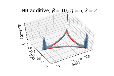
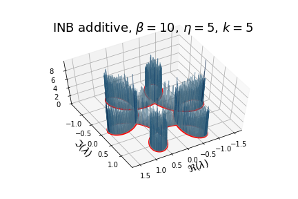
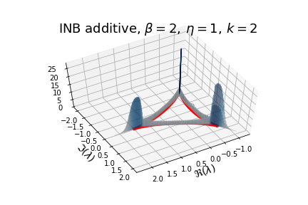
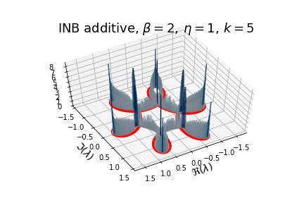
Figure 2: Eigenvalues of INB additive lattice for $k=2$ (left) and $k=5$ (right). $N=1000$ and $6000$ trials performed, in red the corresponding hypotrochoid $\gamma_{+,k}$ defined in equation (92). We observe that the examples on the left panel correspond to the case $\widetilde{\eta}=\frac{\eta}{\beta}=\frac{1}{k}$ that in the limiting case $\eta,\beta\to\infty$ gives the arcsin density of states in (LABEL:nu_infty) where the edges are the cusps of the hypotrochoid. This observation explains the very high peaks located at the cusps.

Another interesting feature of these measures is that their supports seem to be exponentially localized to one dimensional contours. Specifically, it appears that the supports are the two hypotrochoids $\gamma_{+,k},\,\gamma_{\times,k}$, respectively

$$\gamma_{+,k}(t,\eta,\beta)=e^{-it}+\frac{\eta}{\beta}e^{ikt}\,,\qquad\gamma_{\times,k}(t,\eta,\beta)=\frac{\eta}{\beta}e^{-it}+e^{ikt}\,,\quad t\in[0;2\pi)\,.$$ (92)

This feature is highlighted in figures 2-3, where we plot the empirical density of states and the corresponding hypotrochoid. This characteristic is important since this type of curves are also related to the density of some cyclic digraph, see [5], and may serve as a link between these two topics.

All these observations lead us to formulate the following conjecture

Conjecture 1.

Consider the two matrices $L^{(+,k)},\,L^{(\times,k)}$ as in (79), (83) both endowed with the probability distribution $\mathrm{d}\mu_{\textrm{INB}}$ (87). Then, the densities of states $\nu^{\gamma,\beta}_{\textrm{INB},+,k}$ and $\nu^{\gamma,\beta}_{\textrm{INB},\times,k}$ exist, and have a discrete rotational symmetry, namely

$$\nu^{\gamma,\beta}_{\textrm{INB}+,k}(\mathrm{d}z)=\nu^{\gamma,\beta}_{\textrm{INB}+,k}\left(e^{\frac{2\pi i}{k+1}}\mathrm{d}z\right),\qquad\nu^{\gamma,\beta}_{\textrm{INB}\times,k}(\mathrm{d}z)=\nu^{\gamma,\beta}_{\textrm{INB}\times,k}\left(e^{\frac{2\pi i}{k+1}}\mathrm{d}z\right)\,.$$ (93)

Moreover, the densities are exponentially localized in a neighbourhood of the two hypotrochoids $\gamma_{+,k}(t,\eta,\beta)$ and $\gamma_{\times,k}(t,\eta,\beta)$ in (92) respectively.

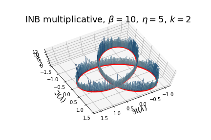
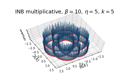
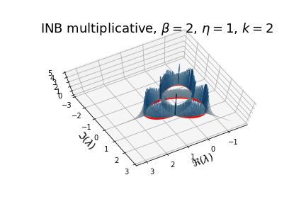
Figure 3: Eigenvalues of INB multiplicative lattice for $k=2$ (left) and $k=5$ (right). $N=1000$ and $6000$ trials performed, in red the corresponding hypotrochoid $\gamma_{\times,k}$

Figure 4: Eigenvalues of INB multiplicative and additive lattice for $k=5$, $N=1000$ and $6000$ trials performed, in red the corresponding hypotrochoid $\gamma_{\times,k},\gamma_{+,k}$

5.2 Parameter limit

As in the previous cases, although we are not able to give an explicit formula for the density of states of the INB lattices for general $\beta,\eta$, we can characterize this measure in the low-temperature limit. Specifically, we consider the limit as $\beta,\eta\to\infty$ in such a way that $\eta=\widetilde{\eta}\beta$, with $\widetilde{\eta}$ in a compact set of $\mathbb{R}_{+}$, and we compute the density of states of the matrices $L^{(+,k)},L^{(\times,k)}$, endowed with the probability inherited from $\mathrm{d}\mu_{\textrm{INB}}$ (87), in this limit.

The procedure is the same as in the case of Volterra (see Section 4.2). Indeed, following the same line, we can conclude that the densities of states $\nu^{\infty}_{\textrm{INB},+,k}$ and $\nu^{\infty}_{\textrm{INB},\times,k}$ coincide with the densities of $\mathfrak{L}^{(+)}$ and $\mathfrak{L}^{(\times)}$ respectively, where

$$\mathfrak{L}^{(+,k)}=\sum_{i=1}^{N}\left(\widetilde{\eta}E_{i+k,i}+E_{i,i+1}\right),\quad\mathfrak{L}^{(\times,k)}=\sum_{i=1}^{N}\left(E_{i+k,i}+\widetilde{\eta}E_{i,i+1}\right)\,.$$ (94)

We notice that both matrices are circulant, thus we can compute their eigenvalues explicitly as

$$\lambda_{j}^{(+,k)}=e^{-2\pi i\frac{j}{N}}+\widetilde{\eta}e^{2\pi i\frac{jk}{N}}\,,\quad\lambda_{j}^{(\times,k)}=\widetilde{\eta}e^{-2\pi i\frac{j}{N}}+e^{2\pi i\frac{jk}{N}}\,,$$ (95)

here $j=1,\ldots,N$. Thus, in the large $N$ limit, we deduce that the support of the measures $\nu^{\infty}_{\textrm{INB}+,k}$ and $\nu^{\infty}_{\textrm{INB}\times,k}$ are the hypotrochoids

$$\gamma_{+,k}(t,\widetilde{\eta},1)=e^{-it}+\widetilde{\eta}e^{ikt}\,,\quad\gamma_{\times,k}(t,\widetilde{\eta},1)=\widetilde{\eta}e^{-it}+e^{ikt}\,,\quad t\in[0;2\pi)\,,$$ (96)

and the limiting eigenvalue densities are

$$\begin{split}&\nu^{\infty}_{\textrm{INB}+,k}=\dfrac{|dz|}{2\pi\sqrt{1+\tilde{\eta}^{2}k^{2}-k(|z|^{2}-1-\tilde{\eta}^{2})}},\quad z\in\gamma_{+,k}\,,\\ &\nu^{\infty}_{\textrm{INB}\times,k}=\dfrac{|dz|}{2\pi\sqrt{\tilde{\eta}^{2}+k^{2}-k(|z|^{2}-1-\tilde{\eta}^{2})}},\quad z\in\gamma_{\times,k}.\end{split}$$ (97)

We summarize these results in the following Proposition.

Proposition 5.4.

The densities of states of the Lax matrices $L^{(+,k)}$ and $L^{(\times,k)}$ in (79) and (83) endowed with the Gibbs measure $\mathrm{d}\mu_{\textrm{INB}}$ in (87), in the low temperature limit, i.e. when $\eta,\,\beta\to\infty$, in such a way that $\eta=\widetilde{\eta}\beta$, with $\widetilde{\eta}$ in a compact set of $\mathbb{R}_{+}$, are given respectively by $\nu^{\infty}_{\textrm{INB}+,k}$ and $\nu^{\infty}_{\textrm{INB}\times,k}$ in (LABEL:nu_infty).

Remark 5.5.

When the parameters satisfy the relation $\widetilde{\eta}k<1$, the curve $\gamma_{+,k}(t,\widetilde{\eta},1)$ is not self-intersecting, while for $\widetilde{\eta}k>1$ the curve is self-intersecting. For $\widetilde{\eta}k=1$ it has cusp singularities [20]. The limiting shape of the support as $\widetilde{\eta}\to 0$ is a circle.
The same considerations are true for the curve $\gamma_{\times,k}(t,\widetilde{\eta})$ upon substitution $\widetilde{\eta}\mapsto 1/\widetilde{\eta}$. We also observe that the density of states $\nu^{\infty}_{\textrm{INB}+,k}$ ( $\nu^{\infty}_{\textrm{INB}\times,k}$) in equation (LABEL:nu_infty) is an Arcsin distribution for $\widetilde{\eta}=\frac{1}{k}$ ($\widetilde{\eta}=k$) and the edges correspond to the cusps of the curve $\gamma_{+,k}(t,\widetilde{\eta})$ ( $\gamma_{\times,k}(t,\widetilde{\eta})$).

6 The focusing Ablowitz-Ladik lattice

The focusing Ablowitz-Ladik lattice is the following system of spatial discrete differential equations

$$i\dot{a}_{j}+a_{j+1}+a_{j-1}-2a_{j}+|a_{j}|^{2}(a_{j-1}+a_{j+1})=0\,,$$ (98)

where $a_{j}\in\mathbb{C},\,j=1,\ldots,N$, $N\geq 3$, and we consider periodic boundary conditions $a_{j+N}=a_{j}$ for all $j\in\mathbb{Z}$. This equation was introduced by Ablowitz and Ladik [1, 2], by searching integrable spatial discretization of the cubic non-linear Schrödinger Equation (NLS) for the complex function $\psi(x,t)$, $x\in\mathbb{R}$, $t\in\mathbb{R}^{+}$

$$i\partial_{t}\psi(x,t)+\partial^{2}_{x}\psi(x,t)+2\lvert\psi(x,t)\rvert^{2}\psi(x,t)=0\,,$$ (99)

In contrast with what happens in the defocusing case, the particles $(a_{1},\dots,a_{N})$ are free to explore the whole $\mathbb{C}^{N}$, which is the phase space of the system.

On the space $\mathcal{C}^{\infty}(\mathbb{C}^{N})$ we consider the Poisson bracket [24, 29]

$$\{f,g\}=i\sum_{j=1}^{N}\rho_{j}^{2}\left(\frac{\partial f}{\partial\overline{a}_{j}}\frac{\partial g}{\partial a_{j}}-\frac{\partial f}{\partial a_{j}}\frac{\partial g}{\partial\overline{a}_{j}}\right)\,,\quad f,g\in\mathcal{C}^{\infty}(\mathbb{C}^{N}).$$ (100)

We notice that the phase shift $a_{j}(t)\to e^{-2it}a_{j}(t)$ transforms the AL lattice (98) into the equation

$$\dot{a}_{j}=i\,\rho_{j}^{2}(a_{j+1}+a_{j-1}),\quad\rho_{j}=\sqrt{1+|a_{j}|^{2}},$$ (101)

which we call the reduced AL equation. We remark that the quantity $H_{0}=2\ln\left(\prod_{j=1}^{N}\rho_{j}^{2}\right)$ is the generator of the shift $a_{j}(t)\to e^{-2it}a_{j}(t)$, while $H_{1}=-K^{(1)}-\overline{K^{(1)}}$ with

$$K^{(1)}:=\sum_{j=1}^{N}a_{j}\overline{a}_{j+1},$$ (102)

generates the flow (101). Therefore, we can rewrite the AL equation as

$$\dot{a}_{j}=\{a_{j},H_{AL}\}\,,\quad H_{AL}=H_{0}+H_{1}\,.$$ (103)

Moreover, it is straightforward to verify that $\{H_{0},H_{1}\}=0$. The Poisson bracket induces the symplectic form

$$\omega=i\sum_{j=1}^{N}\frac{1}{\rho_{j}^{2}}\mathrm{d}a_{j}\wedge\mathrm{d}\overline{a}_{j}\,,\quad\rho_{j}=\sqrt{1+|a_{j}|^{2}}\,,$$ (104)

that is invariant under the evolution generated by the Hamiltonians $H_{0}$ and $H_{1}$. Therefore, the volume form

$$\omega^{N}=\omega\wedge\dots\wedge\omega,$$

is also invariant. In view of these properties, we can define the Gibbs ensemble for the focusing Ablowitz-Ladik lattice on the phase space $\mathbb{C}^{N}$ as

$$\mathrm{d}\mu_{AL}=\frac{1}{Z_{N}^{AL}(\beta)}e^{\frac{\beta}{2}H_{0}}\omega^{N}=\frac{1}{Z_{N}^{AL}(\beta)}\prod_{j=1}^{N}\left(1+|a_{j}|^{2}\right)^{-\beta-1}\mathrm{d}^{2}\mathbf{a}\,,\quad\beta>0\,,$$ (105)

where $\mathbf{a}=(a_{1},\ldots,a_{N})$, $\mathrm{d}^{2}\mathbf{a}=\prod_{j=1}^{N}(i\mathrm{d}a_{j}\wedge\mathrm{d}\overline{a}_{j})$ and $Z_{N}^{AL}(\beta)$ is the normalization constant of the system. We notice that according to this measure, all the variables are i.i.d.

Remark 6.1.

The measure with density $\exp(-\beta H_{AL})$ and $\beta>0$ is not bounded nor normalizable on the whole phase space. For this reason, we have defined the Gibbs ensemble as in (105). Furthermore, we observe that the measure (105) has a finite number of moments, which implies that the corresponding density of states of the Lax matrix (see (108) below), if it exists, would have a finite number of moments.

The focusing AL lattice is a complete integrable system. Indeed it admits a Lax representation, first obtained by Ablowitz and Ladik from the discretization of the Zakharov-Shabat Lax pair for the focusing non-linear Schrödinger equation [63]. Gesztesy, Holden, Michor, and Teschl [30] found a different Lax pair for the infinite case of focusing AL lattice, and for its general hierarchy. To adapt their construction, we double the size of the lattice according to the periodic boundary conditions, thus we consider a chain of $2N$ particles $a_{1},\ldots,a_{2N}$ such that $a_{j}=a_{j+N}$ for $j=1,\ldots,N$. Define the $2\times 2$ matrix $\Xi_{j}$

$$\Xi_{j}=\begin{pmatrix}-a_{j}&\rho_{j}\\ \rho_{j}&-\overline{a_{j}}\end{pmatrix}\,,\quad j=1,\dots,2N\,,$$ (106)

and the $2N\times 2N$ matrices

$$\mathcal{M}=\begin{pmatrix}-\overline{a_{2N}}&&&&&\rho_{2N}\\ &\Xi_{2}\\ &&\Xi_{4}\\ &&&\ddots\\ &&&&\Xi_{2N-2}\\ \rho_{2N}&&&&&-a_{2N}\end{pmatrix}\,,\qquad\mathcal{L}=\begin{pmatrix}\Xi_{1}\\ &\Xi_{3}\\ &&\ddots\\ &&&\Xi_{2N-1}\end{pmatrix}\,.$$ (107)

Now let us define the Lax matrix

$$\mathcal{E}=\mathcal{L}\mathcal{M}\,,$$ (108)

that has the structure of a $5$-band diagonal matrix

$$\begin{pmatrix}*&*&*&&&&&&&*\\ *&*&*&&&&&&&*\\ &*&*&*&*&&&&&\\ &*&*&*&*&&&&&\\ &&&&&\ddots&\ddots&&&\\ &&&&&&*&*&*&*\\ &&&&&&*&*&*&*\\ *&&&&&&&*&*&*\\ *&&&&&&&*&*&*\\ \end{pmatrix}\,.$$

The $N$-periodic equation (101) is equivalent to the following Lax equation for the matrix $\mathcal{E}$,

$$\dot{\mathcal{E}}=\left[\mathcal{A},\mathcal{E}\right]\,,$$ (109)

where

$$\mathcal{A}=\frac{i}{2}(\mathcal{E}_{+}-\mathcal{E}_{-}-\mathcal{E}_{+}^{-1}+\mathcal{E}^{-1}_{-})\,,$$ (110)

where the two projections $M_{+},\,M_{-}$ are defined for a $2N\times 2N$ matrix as

$$M_{+}=\begin{cases}M_{\ell,j}\,,\quad\ell<j\leq\ell+N\\ M_{\ell,j}\,,\quad\ell>j+N\\ 0\quad\textrm{otherwise}\end{cases}\,,\quad M_{-}=\begin{cases}M_{\ell,j}\,,\quad j<\ell\leq j+N\\ M_{\ell,j}\,,\quad j>\ell+N\\ 0\quad\textrm{otherwise}\end{cases}\,.$$ (111)

We notice that the Lax matrix $\mathcal{E}$ has a similar structure to the one of the defocusing AL lattice obtained by Nenciu, and Simon [53, 55]. The crucial difference is that while for the defocusing AL lattice the blocks $\Xi_{j}$ are unitary matrices, for the focusing lattice this is not the case since $\Xi_{j}\Xi_{j}^{\dagger}\neq I_{2}$ where $I_{2}=\begin{pmatrix}1&0\\ 0&1\end{pmatrix}$ and ^† stands for hermitian conjugate.

The measure $\mathrm{d}\mu_{AL}$ induces a probability distribution on the entries of the matrix $\mathcal{E}$, thus it becomes a random matrix. As in the previous cases, one would like to connect the density of states for this random matrix to the density of states of some $\beta$-ensemble in the high temperature regime, but, as in the case of the INB lattices, we lack of a matrix representation of some $\beta$-ensemble with eigenvalues supported on the plane.

We make the following observations. The matrix $\Xi_{j}$ (106) is complex symmetric, and it can be factorized in the form

$$\Xi_{j}=U_{j}\begin{pmatrix}\frac{\overline{a_{j}}}{|a_{j}|\left(|a_{j}|+\sqrt{1+|a_{j}|^{2}}\right)}&0\\ 0&-\frac{a_{j}}{|a_{j}|}(|a_{j}|+\sqrt{1+|a_{j}|^{2}})\end{pmatrix}U_{j}$$ (112)

where the matrices $U_{j}=\begin{pmatrix}\frac{a_{j}}{\sqrt{2}|a_{j}|}&\frac{1}{\sqrt{2}}\\ \frac{1}{\sqrt{2}}&-\frac{\overline{a_{j}}}{\sqrt{2}|a_{j}|}\end{pmatrix}$ are unitary, $U_{j}^{-1}=U_{j}^{\dagger}$. Thus defining the matrices

$$\widetilde{\mathcal{M}}=\begin{pmatrix}-\frac{\overline{a_{2N}}}{\sqrt{2}|a_{2N}|}&&&&&\frac{1}{\sqrt{2}}\\ &U_{2}\\ &&U_{4}\\ &&&\ddots\\ &&&&U_{2N-2}\\ \frac{1}{\sqrt{2}}&&&&&\frac{a_{2N}}{\sqrt{2}|a_{2N}|}\end{pmatrix}\,,\qquad\widetilde{\mathcal{L}}=\begin{pmatrix}U_{1}\\ &U_{3}\\ &&\ddots\\ &&&U_{2N-1}\end{pmatrix}\,,$$ (113)

we can rewrite the Lax matrix $\mathcal{E}$ (108) as

$$\mathcal{E}=\widetilde{\mathcal{L}}\Lambda_{\text{odd}}\widetilde{\mathcal{L}}\widetilde{\mathcal{M}}\Lambda_{\text{even}}\widetilde{\mathcal{M}}\,,$$ (114)

where, defining $c_{j}:=\frac{\overline{a_{j}}}{|a_{j}|\left(|a_{j}|+\sqrt{1+|a_{j}|^{2}}\right)}$, the matrices $\Lambda_{\text{odd}}$ and $\Lambda_{\text{even}}$ are given by

$$\begin{split}&\Lambda_{\text{odd}}=\operatorname{diag}\left(c_{1},-\frac{1}{c_{1}},c_{3},-\frac{1}{c_{3}},\dots,c_{2N-1},-\frac{1}{c_{2N-1}}\right)\\ &\Lambda_{\text{even}}=\operatorname{diag}\left(-\frac{1}{c_{2N}},c_{2},-\frac{1}{c_{2}},\ldots,c_{2N}\right)\,.\end{split}$$ (115)

Since we are interested in the distribution of the eigenvalues of $\mathcal{E}$, it follows from the factorization (114) that we can also consider the matrix $\Lambda_{\text{odd}}\widetilde{\mathcal{E}}\Lambda_{\text{even}}\widetilde{\mathcal{E}}^{\intercal}$, where $\widetilde{\mathcal{E}}=\widetilde{\mathcal{L}}\widetilde{\mathcal{M}}$. The eigenvalues of $\Lambda_{\text{even}},\Lambda_{\text{odd}}$ come in pairs, such that if $\lambda$ is an eigenvalue, then also $-\lambda^{-1}$ is an eigenvalue. The matrix $\widetilde{\mathcal{E}}$ is a periodic CMV matrix [18], thus its eigenvalues are on the unit circle.

Thus, we are in a similar setting considered in [59, 60, 34]. Indeed in [59] the authors derived the eigenvalues distribution of $U\sqrt{D}$ where $U$ is a Haar distributed unitary matrix and $D$ is a fixed diagonal matrix with positive eigenvalues. They show that the density of states is rotational invariant and it is supported on a single ring whose radii $r_{1}<r_{2}$ satisfy the constraint $d_{min}<r_{1}<r_{2}<d_{max}$, where $d_{min}$ and $d_{max}$ are the minimum and maximum eigenvalues of $D$. In [34], the authors considered a similar problem, namely the characterization of the density of states for a matrix of the form $UTV$, where $U,V$ are independent unitary matrices Haar distributed, and $T$ is a real diagonal matrix independent of $U,V$. They proved, under some mild conditions, that the density of states of the matrix $UTV$ is radially symmetric and it is supported on a ring.

It is therefore reasonable to expect that the density of states of the random Lax matrix of the Ablowitz-Ladik lattice is rotational invariant, but with unbounded support, indeed the eigenvalues of $\Lambda_{\text{even}},\Lambda_{\text{odd}}$ could grow to infinity.

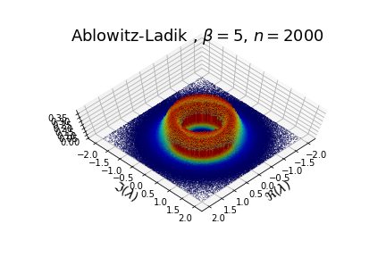
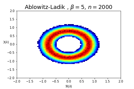
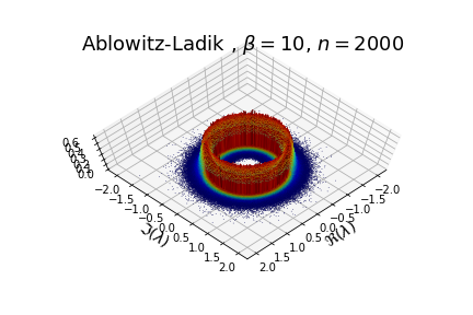
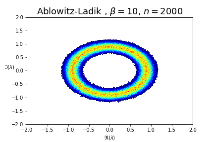
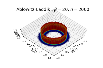
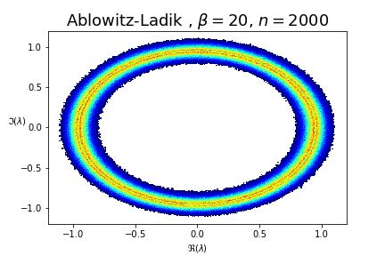
Figure 5: Empirical densities for the focusing Ablowitz-Ladik lattice for $\beta=5,10,20$, $10000$ trials per picture .

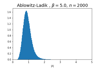
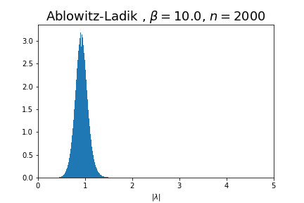
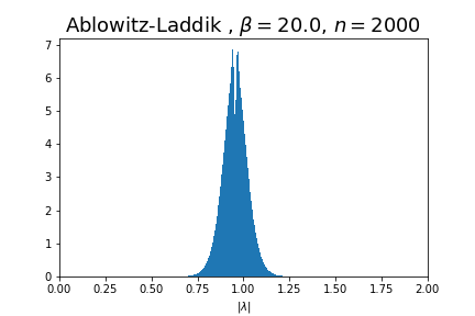
Figure 6: Empirical density for the eigenvalues’ modulus for the focusing Ablowitz-Ladik lattice for $\beta=5,10,20$, $10000$ trials per picture.

To confirm our expectations, we perform several numerical investigations of the eigenvalues of the random Lax matrix of the Ablowitz-Ladik lattice for various values of $\beta$ (see Fig 5-6). In Fig 5 the eigenvalue density is shown. As expected, the density seems to be rotational invariant, and concentrated on a ring, exactly as in [59, 60, 34]. For this reason, we investigate the behaviour of the modulus of the eigenvalues, see Fig 6. They seem to be concentrated in a small region, but, in view of Remark 6.1, we expect that the tails should decay just polynomially fast.

6.1 Parameter Limit

Despite not being able to explicitly compute the density of states for general values of $\beta$, we can perform such an analysis in the low-temperature limit, namely when $\beta\to\infty$.

We notice that, according to (105), all the $a_{j}$ are independent. Hence, in order to obtain the density of states in the low-temperature limit, we have to compute the weak limit of the density

$$\mathrm{d}\mu_{\beta}=\frac{(1+|z|^{2})^{-\beta-1}\mathrm{d}z}{\int_{\mathbb{D}}(1+|z|^{2})^{-\beta-1}\mathrm{d}z}\,.$$ (116)

Proceeding as in the previous cases, it follows that the following limit holds for all bounded and continuous $f\;:\overline{\mathbb{D}}\to\mathbb{R}$:

$$\lim_{\beta\to\infty}\int_{\mathbb{D}}f(z)\mathrm{d}\mu_{\beta}=f(0)$$ (117)

The previous limit implies that the density of states of the Ablowitz-Ladik lattice in the low temperature limit is equal to the one of $\widehat{\mathcal{E}}=\widehat{\mathcal{L}}\widehat{\mathcal{M}}$, where $\widehat{\mathcal{L}},\,\widehat{\mathcal{M}}$ are $2N\times 2N$ matrices

$$\widehat{\mathcal{M}}=\begin{pmatrix}0&&&&&1\\ &\widetilde{\Xi}\\ &&\widetilde{\Xi}\\ &&&\ddots\\ &&&&\widetilde{\Xi}\\ 1&&&&&0\end{pmatrix}\,,\qquad\widehat{\mathcal{L}}=\begin{pmatrix}\widetilde{\Xi}\\ &\widetilde{\Xi}\\ &&\ddots\\ &&&\widetilde{\Xi}\end{pmatrix}\,,$$ (118)

and $\widehat{\Xi}$ is defined as the unitary matrix

$$\widehat{\Xi}=\begin{pmatrix}0&1\\ 1&0\end{pmatrix}\,.$$ (119)

To compute the density of states for the matrix $\mathcal{E}$, we notice that both $\widehat{\mathcal{M}}$, and $\widehat{\mathcal{L}}$ are permutation matrices. Specifically, we identify them with the following permutations

$$\begin{split}&\widehat{\mathcal{M}}\longleftrightarrow(2N,1)(2,3)(4,5)\ldots(2N-2,2N-1)\,,\\ &\widehat{\mathcal{L}}\longleftrightarrow(1,2)(3,4)(5,6)\ldots(2N-1,2N)\,.\end{split}$$ (120)

As a consequence, the matrix $\widehat{\mathcal{E}}$ itself corresponds to the permutation

$$\widehat{\mathcal{E}}\longleftrightarrow(1,3,5,\ldots,2N-1)(2,4,6,\ldots,2N)\,.$$ (121)

This implies that the eigenvalues of $\widehat{\mathcal{E}}$ are all double, and given by

$$\lambda_{j}=e^{2\pi i\frac{j}{N}}\,,\quad j=1,\ldots,2N\,.$$

From this explicit expression of the eigenvalues, it is straightforward to prove that

$$\nu_{AL}=\frac{\mathrm{d}\theta}{2\pi}\,,\quad\theta\in[0,2\pi)\,.$$ (122)

Thus, we have proved the following

Proposition 6.2.

Consider the Gibbs ensemble $\mathrm{d}\mu_{AL}$ (105) of the focusing Ablowitz-Ladik lattice in the low-temperature limit, i.e. $\beta\to\infty$. Then, the density of states $\nu_{AL}$ of the Lax matrix $\mathcal{E}$ (108) is given by

$$\nu_{AL}=\frac{\mathrm{d}\theta}{2\pi}\,,\quad\theta\in[0,2\pi)\,.$$ (123)

7 Schur flow

The focusing Schur flow, also known as discrete mKdV, is an integrable system deeply related to the Ablowitz-Ladik lattice. Its equations of motion are

$$\dot{a}_{j}=\rho_{j}^{2}(a_{j+1}-a_{j-1})\,,\quad\rho_{j}=\sqrt{1+|a_{j}|^{2}}\,,$$ (124)

where here we consider periodic boundary conditions, $a_{j}=a_{j+N}$ for all $j\in\mathbb{Z}$. Notice that if $a_{j}(0)\in\mathbb{R}$ for all $j=1,\ldots,N$, then $a_{j}(t)\in\mathbb{R}$ for all times, implying that $\mathbb{R}^{N}$ is an invariant subspace for the dynamics.

Recalling the definition (102) for $K^{(1)}=\sum_{j=1}^{N}a_{j}\overline{a}_{j+1}$ and introducing the Poisson bracket

$$\{f,g\}=\sum_{j=1}^{N}\rho_{j}^{2}\left(\frac{\partial f}{\partial\overline{a}_{j}}\frac{\partial g}{\partial a_{j}}-\frac{\partial f}{\partial a_{j}}\frac{\partial g}{\partial\overline{a}_{j}}\right)\,,\quad f,g\in\mathcal{C}^{\infty}(\mathbb{C}^{N}),$$ (125)

we can rewrite the equations of motion (124) as

$$\dot{a}_{j}=\{a_{j},H_{S}\}\,,\quad H_{S}=K^{(1)}-\overline{K^{(1)}}\,.$$ (126)

Notice that the quantity $H_{0}=-2\ln\left(\prod_{j=1}^{N}\rho_{j}^{2}\right)$ is a global first integral for the system. Moreover, one can deduce immediately from the equations of motion that $\mathbb{R}^{N}$ is invariant for the dynamics. Thus, in view of the Hamiltonian representation and this invariance, we define the Gibbs measure for the Schur flow as

$$\mathrm{d}\mu_{S}=\frac{1}{Z_{N}^{S}(\beta)}\prod_{j=1}^{N}\left(1+a_{j}^{2}\right)^{-\beta-1}\mathrm{d}\mathbf{a}\,,\quad a_{j}\in\mathbb{R}\,,$$ (127)

where $Z_{N}^{S}(\beta)$ is the normalization constant of the system,

$$Z_{N}^{S}(\beta)=\int_{\mathbb{R}^{N}}\prod_{j=1}^{N}\left(1+a_{j}^{2}\right)^{-\beta-1}\mathrm{d}\mathbf{a}\,.$$ (128)

Remark 7.1.

Similarly to the focusing AL case, the classical Gibbs ensemble is not well-defined on the whole phase space. Indeed, the measure with density $e^{-\beta H_{S}}$, $\beta>0$ cannot be normalized on $\mathbb{R}^{N}$.

The Schur flow is a completely integrable system since it admits a Lax formulation. Namely, define the $2\times 2$ matrix $\Xi_{j}$

$$\Xi_{j}=\begin{pmatrix}-a_{j}&\rho_{j}\\ \rho_{j}&-\overline{a_{j}}\end{pmatrix}\,,\quad j=1,\dots,2N\,,$$ (129)

and, similarly to the Ablowitz-Ladik case, the $2N\times 2N$ matrices

$$\mathcal{M}=\begin{pmatrix}-\overline{a_{2N}}&&&&&\rho_{2N}\\ &\Xi_{2}\\ &&\Xi_{4}\\ &&&\ddots\\ &&&&\Xi_{2N-2}\\ \rho_{2N}&&&&&-a_{2N}\end{pmatrix}\,,\qquad\mathcal{L}=\begin{pmatrix}\Xi_{1}\\ &\Xi_{3}\\ &&\ddots\\ &&&\Xi_{2N-1}\end{pmatrix}\,.$$ (130)

Then, the $N$-periodic equation (124) is equivalent to the following Lax equation for the matrix $\mathcal{E}$:

$$\dot{\mathcal{E}}=\left[\mathcal{A},\mathcal{E}\right]\,,$$ (131)

where

$$\mathcal{A}=\frac{1}{2}\left(\mathcal{E}_{+}+\mathcal{E}_{+}^{-1}-\mathcal{E}_{-}-\mathcal{E}_{-}^{-1}\right)\,,$$ (132)

where the two projection $+,-$ are defined in (111).

Carrying on with the approach of this article, we study the density of states $\nu_{S}$ for the matrix $\mathcal{E}$ when the entries are distributed according to the measure (127). First, we notice that Remark 6.1 is valid also in the case of the focusing Schur flow. Moreover, since the variables $a_{j}$ are real, we can factorize the matrices $\Xi_{j}$ in the following way:

$$\Xi_{j}=U_{0}\operatorname{diag}\left(c_{j},-\frac{1}{c_{j}}\right)U_{0},\,\quad c_{j}=\sqrt{1+a_{j}^{2}}-a_{j},\,\quad U_{0}=\frac{1}{\sqrt{2}}\begin{pmatrix}1&1\\ 1&-1\end{pmatrix},$$ (133)

where we note that $U_{0}^{-1}=U_{0}$, so that the above is a similarity transformation. Thus, defining

$$\widetilde{\mathcal{M}}=\begin{pmatrix}-\frac{1}{\sqrt{2}}&&&&&\frac{1}{\sqrt{2}}\\ &U_{0}\\ &&U_{0}\\ &&&\ddots\\ &&&&U_{0}\\ \frac{1}{\sqrt{2}}&&&&&\frac{1}{\sqrt{2}}\end{pmatrix}\,,\qquad\widetilde{\mathcal{L}}=\begin{pmatrix}U_{0}\\ &U_{0}\\ &&\ddots\\ &&&U_{0}\end{pmatrix}\,,$$ (134)

we can rewrite the Lax matrix of the Schur flow $\mathcal{E}$ as

$$\mathcal{E}=\widetilde{\mathcal{L}}\Lambda_{\text{odd}}\widetilde{\mathcal{L}}\widetilde{\mathcal{M}}\Lambda_{\text{even}}\widetilde{\mathcal{M}}\,,$$ (135)

where

$$\begin{split}&\Lambda_{\text{odd}}=\operatorname{diag}\left(c_{1},-\frac{1}{c_{1}},c_{3},\ldots\right)\,,\\ &\Lambda_{\text{even}}=\operatorname{diag}\left(-\frac{1}{c_{2N}},c_{2},\ldots,c_{2N}\right)\,.\end{split}$$ (136)

As in the case of the Ablowitz-Ladik lattice, since we are interested in just the distribution of the eigenvalues of $\mathcal{E}$, we can consider the matrix $\Lambda_{\text{odd}}\widetilde{\mathcal{E}}\Lambda_{\text{even}}\widetilde{\mathcal{E}}^{\intercal}$, where

$$\widetilde{\mathcal{E}}=\widetilde{\mathcal{L}}\widetilde{\mathcal{M}}.$$ (137)

As in the AL case, the eigenvalues of $\Lambda_{\text{even}},\Lambda_{\text{odd}}$ come in pairs, such that if $\lambda$ is an eigenvalue, then also $-\lambda^{-1}$ is an eigenvalue. The main difference with the case of the focusing AL lattice is that in this case the matrix $\widetilde{\mathcal{E}}$ is deterministic. Thus, one can be led to think that the eigenvalue distribution of the Schur flow would be similar to the one of the AL lattice, but it is not the case. Indeed, we perform several numerical investigations, reported in Fig 7, which shows that the behaviour of the eigenvalues is different in the two situations.

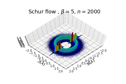
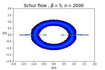
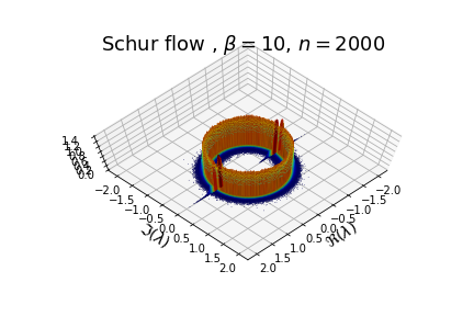
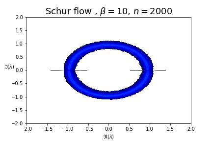
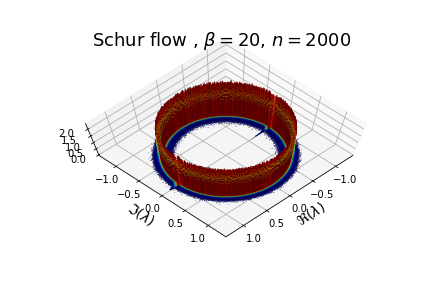
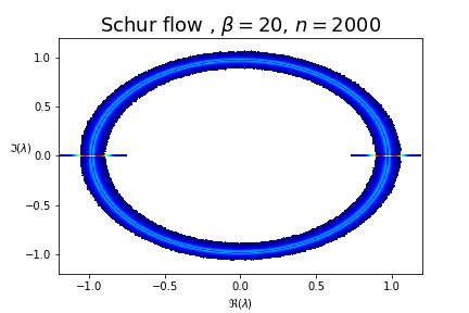
Figure 7: Schur flow eigenvalue density for $\beta=5,10,20$, $10000$ trials.

We notice that a consistent part of the eigenvalues tend to stay close to the real axis, see Fig 7. This behaviour is also typical of the orthogonal Ginibre ensemble [23]. The main reason is that the eigenvalues of $\widetilde{\mathcal{E}}$ are not evenly spaced on the unit circle, but they are constrained to the left semicircle, and are more dense nearby $\pm i$ (see Fig 8). Indeed we can give an accurate description of the spectrum of this matrix.

More precisely, we have the following.

Proposition 7.2.

Let $\widetilde{\mathcal{E}}$ be the $2N\times 2N$ matrix defined in (137). Its eigenvalues are the solutions of the quadratic equations

$$\lambda+\frac{1}{\lambda}+1=\cos\left(\frac{2\pi j}{N}\right),\quad\quad j=0,1,\dots,N-1,$$ (138)

counting the multiplicity.

Proof.

See Appendix A. ∎

Remark 7.3.

From equation (138) we can infer the limiting distributions of the eigenvalues of $\widetilde{\mathcal{E}}$. We already know all of its eigenvalues lie in the unit circle, hence we can write $\lambda=e^{i\varphi}$ for some $\varphi\in[-\pi,\pi)$. Equation (138) thus becomes

$$e^{i\varphi}+e^{-i\varphi}+1=\cos\left(\frac{2\pi j}{N}\right)\quad\iff\quad\varphi=\arccos\left(\frac{1}{2}\cos\left(\frac{2\pi j}{N}\right)-\frac{1}{2}\right).$$ (139)

Passing to the limit $N\to\infty$, by standard methods, we can compute the limiting density of the argument $\varphi$ of the eigenvalues as

$$\mu(\varphi)\mathrm{d}\varphi=\left(\mathbbm{1}_{[\frac{\pi}{2},\pi]}(\varphi)-\mathbbm{1}_{[-\pi,-\frac{\pi}{2}]}(\varphi)\right)\frac{\sin{\varphi}\,\mathrm{d}\varphi}{\pi\sqrt{1-\left(1+2\cos{\varphi}\right)^{2}}}$$ (140)

This behaviour is shown in Fig 8.

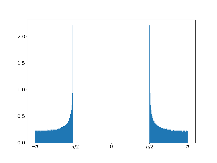
Figure 8: Distribution of the eigenvalues arguments for the $\widetilde{\mathcal{E}}$ (137), $N=5000$.

Furthermore, as in the case of the AL lattice, for large $\beta$ the eigenvalues tend to accumulate on the unit circle, see Fig 7. In a similar way as done for the focusing AL lattice we conclude that the density of states of the random Lax matrix $\mathcal{E}$ in (108) with probability distribution entries given by the Gibbs measure $\mathrm{d}\mu_{S}$ in (127), converge in the limit $\beta\to\infty$ to the uniform measure on the unit circle.

8 Conclusions and outlook

In this manuscript, we underlined the deep relation between integrable systems and random matrix theory. Specifically, we showed that the exponential Toda lattice, and the Volterra one are related to the Laguerre $\beta$-ensemble at high temperature and the antisymmetric Gaussian $\beta$-ensemble at high temperature respectively. As we already mentioned in the introduction, these are not isolated and lucky relations, indeed the Toda lattice is related to the Gaussian $\beta$-ensemble at high temperature, and the Ablowitz-Ladik one to the Circular $\beta$ ensemble. Thus, in view of the new relations that we obtained, we conclude that each classical $\beta$-ensemble in the high temperature regime is related to some integrable model, see Table 1.

Furthermore, we numerically investigate the additive and multiplicative INB lattices, which are a generalization of the Volterra one. Since the former lattice is related to the antisymmetric Gaussian $\beta$-ensemble, it may be possible that the INB lattice could be related to some generalization of the antisymmetric Gaussian $\beta$-ensemble themselves.

Finally, we considered the focusing Ablowitz-Ladik lattice and the focusing Schur flow. In view of our numerical investigations, we were able to formulate a precise conjecture regarding the eigenvalues distribution of the focusing Ablowitz-Ladik lattice. Considering the focusing Schur flow, we were not able to formulate a precise conjecture for its eigenvalues distribution. The expectation is that it would be related to the a possible Ginibre $\beta$-ensemble.

It would be fascinating to consider the generalized Gibbs ensemble for the exponential Toda lattice and the Volterra one, and prove that both their empirical measures satisfy a Large Deviation principle in the spirit of [35, 49]. Moreover, it would be interesting to apply the theory of Generalized Hydrodynamic [13] to have some insight regarding the behaviour of the correlation functions for these systems.

$\beta$-ensemble at high temperature	Integrable System
Gaussian	Toda lattice
Laguerre	Exponential Toda lattice
Jacobi	Defocusing Schur flow
Circular	Defocusing Ablowitz-Ladik lattice
Antisymmetric Gaussian	Volterra lattice

Table 1: $\beta$-ensembles and integrable systems

Appendix A Proof of Proposition 7.2

Recall that the matrix $\widetilde{\mathcal{E}}$ is defined as $\widetilde{\mathcal{E}}=\widetilde{\mathcal{L}}\widetilde{\mathcal{M}}$ where $\widetilde{\mathcal{L}}$ and $\widetilde{\mathcal{M}}$ are as in (134). It is a block circulant matrix, indeed we can write

$$\widetilde{\mathcal{E}}=\frac{1}{2}\begin{pmatrix}E_{0}&E_{1}&&&E_{-1}\\ E_{-1}&E_{0}&E_{1}&&\\ &\ddots&\ddots&\ddots&\\ &&\ddots&\ddots&E_{1}\\ E_{1}&&&E_{-1}&E_{0}\end{pmatrix},$$ (141)

with

$$E_{0}=\begin{pmatrix}-1&1\\ -1&-1\end{pmatrix},\qquad E_{-1}=\begin{pmatrix}0&1\\ 0&1\end{pmatrix},\qquad E_{1}=\begin{pmatrix}1&0\\ -1&0\end{pmatrix}.$$ (142)

One can immediately check that $\lambda=\pm i$ are eigenvalues for $\widetilde{\mathcal{E}}$ with eigenvectors

$$v_{\pm i}=\left(\mp i,1,\mp i,1,\dots,\mp i,1\right)^{\intercal}.$$ (143)

We now claim that, for fixed $N$, the remaining eigenvalues have multiplicity 2 and are the $(N-1)$ solutions to $\Omega\left(\lambda\right)^{N}=I_{2}$, where we defined

$$\Omega\left(\lambda\right)=\begin{pmatrix}\lambda&-\lambda-1\\ -\lambda-1&\frac{\lambda^{2}+2\lambda+2}{\lambda}\end{pmatrix}.$$ (144)

Such solutions are obtained by solving the equation

$$\lambda+\frac{1}{\lambda}+1=\cos\left(\frac{2\pi j}{N}\right)\qquad for\;\ j=0,\dots,\left\lfloor\frac{N}{2}\right\rfloor\,.$$ (145)

For $j=0$ the solutions to (145) are $\pm i$ which we already treated separately. Indeed $\Omega\left(\pm i\right)$ is not diagonalizable and $\Omega\left(\pm i\right)^{N}\neq I_{2}$ for every $N$ greater than 0. For any other $j\in\{1,\dots,\left\lfloor\frac{N}{2}\right\rfloor\}$, the solutions to (145) are

$$\lambda_{1,2}=\frac{\cos\left(\frac{2\pi j}{N}\right)-1}{2}\pm i\frac{\sqrt{3+2\cos\left(\frac{2\pi j}{N}\right)-\cos^{2}\left(\frac{2\pi j}{N}\right)}}{2}.$$ (146)

Since both the real and imaginary part are monotone functions of $j$, different $j^{\prime}s$ will correspond to different solutions. Hence, if $N$ is odd, we will have a total of $N-1$ solutions coming from (146); if $N$ is even one has $N-2$ distinct solutions coming from the equation in (145) plus the double solution $\lambda=-1$ obtained for $j=N/2$.

For a given eigenvalue $\lambda$, the corresponding independent eigenvectors are

$$v_{1} =\left((1,0)\Omega\left(\lambda\right),\dots,\,(1,0)\Omega\left(\lambda\right)^{N-1},1,0\right)^{\intercal},$$ (147)

$$v_{2} =\left((0,1)\Omega\left(\lambda\right),\dots,\,(0,1)\Omega\left(\lambda\right)^{N-1},0,1\right)^{\intercal}\,.$$ (148)

Let us check the correctness of the claim. Write $\widetilde{\mathcal{E}}v_{1}:=(w_{1},\dots,w_{N})^{\intercal}$, where $w_{j}$ are two-dimensional row vectors, then using the fact that $\Omega\left(\lambda\right)^{N}=I_{2}$, one can compute for any $k=1,\dots,N$,

$$w_{k}^{\intercal} =\frac{1}{2}\left(E_{-1}\,\Omega\left(\lambda\right)^{-1}+E_{0}+E_{1}\,\Omega\left(\lambda\right)\right)\Omega\left(\lambda\right)^{k}\begin{pmatrix}1\\ 0\end{pmatrix}$$ (149)

$$=\frac{1}{2}\left(\begin{pmatrix}\lambda+1&\lambda\\ \lambda+1&\lambda\end{pmatrix}+\begin{pmatrix}-1&1\\ -1&-1\end{pmatrix}+\begin{pmatrix}\lambda&-\lambda-1\\ -\lambda&\lambda+1\end{pmatrix}\right)\Omega\left(\lambda\right)^{k}\begin{pmatrix}1\\ 0\end{pmatrix}$$ (150)

$$=\lambda\cdot\Omega\left(\lambda\right)^{k}\begin{pmatrix}1\\ 0\end{pmatrix},$$ (151)

which shows that $v_{1}$ is an eigenvector with eigenvalue $\lambda$. The same proof clearly applies to the other eigenvector $v_{2}$.

Appendix B Confluent Hypergeometric Functions

B.1 Tricomi Confluent Hypergeometric function

The Tricomi Confluent Hypergeometric function $\psi(a,b;z)$, that we introduced in Theorem 3.1, is defined as the solution of the Kummer’s equation

$$z\frac{\mathrm{d}^{2}\psi}{\mathrm{d}z^{2}}+(b-z)\frac{\mathrm{d}\psi}{\mathrm{d}z}-a\psi=0\,,$$ (152)

such that

$$\psi(a,b;z)\sim z^{-a}\,,\quad z\to\infty\,,|\arg(z)|\leq\frac{3}{2}\pi-\delta\,,$$ (153)

here $\delta$ is a small positive constant. The origin is a regular singular point for this equation with indexes $0$ and $1-b$, moreover, this equation has an irregular singularity at infinity of rank one. Usually, $\psi(a,b;z)$ has a branch point at $0$, whose principal branch is the same as $z^{-a}$, thus it has a cut on the $z$ plane along the interval $(-\infty,0]$.

B.2 Whittaker function

The Whittaker function $W_{\mu,\kappa}(z)$, that we introduced in Theorem 4.2, is defined as the solution to the Whittaker’s equation

$$\frac{\mathrm{d}^{2}W}{\mathrm{d}z^{2}}+\left(-\frac{1}{4}+\frac{\kappa}{z}+\frac{1-4\mu^{2}}{4z^{2}}\right)W=0\,,$$ (154)

such that

$$W_{\mu,\kappa}(z)\sim e^{-\frac{z}{2}}z^{\kappa}\,,\quad z\to\infty\,,|\arg(z)|\leq\frac{3}{2}\pi-\delta\,,$$ (155)

here $\delta$ is a small positive constant. The Whittaker’s equation is obtained from Kummer’s equation (152) via the substitution $W=e^{-\frac{z}{2}}z^{\frac{1}{2}+\mu}\psi(a,b;z)$, with $\kappa=\frac{1}{2}(b-a)$, and $\mu=\frac{1}{2}(b-1)$. It has a regular singularity at $0$ with index $\frac{1}{2}\pm\mu$, and an irregular singularity at infinity of rank $1$. Moreover, the following equality holds

$$W_{\mu,\kappa}(z)=e^{-\frac{z}{2}}z^{\frac{1}{2}+\mu}\psi\left(\frac{1}{2}+\mu-\kappa,1+2\mu;z\right)\,.$$ (156)

For a more general overview on Confluent Hypergeometric functions, we refer to [19, §13], and [4, Chapter 13].

Data Availability Statement

The python program to generate figures 2–8 can be found at [47].

Conflict of Interest Statement

The authors declare no conflict of interest.

Funding

This work was supported bu Marie Sklodowska–Curie grant No. 778010 IPaDEGAN Moreover, G.M. is financed by the KAM grant number 2018.0344.

References

- [1] M. J. Ablowitz and J. F. Ladik, Nonlinear differential-difference equations, J. Math. Phys., 16 (1974), pp. 598–603.
- [2] , Nonlinear differential-difference equations and Fourier analysis, J. Math. Phys., 17 (1975), pp. 1011–1018.
- [3] M. J. Ablowitz and H. Segur, Solitons and the Inverse Scattering Transform, Society for Industrial and Applied Mathematics, Philadelphia, 1981.
- [4] M. Abramowitz and I. A. Stegun, Handbook of mathematical functions with formulas, graphs, and mathematical tables, National Bureau of Standards Applied Mathematics Series, No. 55, U. S. Government Printing Office, Washington, D.C., 1964. For sale by the Superintendent of Documents.
- [5] P. V. Aceituno, T. Rogers, and H. Schomerus, Universal hypotrochoidic law for random matrices with cyclic correlations, Phys. Rev. E, 100 (2019), p. 010302.
- [6] R. Allez, J. P. Bouchaud, and A. Guionnet, Invariant beta ensembles and the Gauss-Wigner crossover, Phys. Rev. Lett., 109 (2012), pp. 1–5.
- [7] R. Allez, J.-P. Bouchaud, S. N. Majumdar, and P. Vivo, Invariant -Wishart ensembles, crossover densities and asymptotic corrections to the Marčenko-Pastur law, J. Phys. A, 46 (2013), pp. 015001, 22.
- [8] V. I. Arnol’d, On a theorem of Liouville concerning integrable problems in dynamics, Amer. Math. Soc. Trasl., 61 (1967), pp. 292–296.
- [9] , Dynamical Systems III, vol. 3 of Encyclopaedia of Mathematical Sciences, Springer-Verlag, Berlin, 1987.
- [10] , Mathematical Methods of Classical Mechanics, vol. 60 of Graduate Texts in Mathematics, Springer-Verlag, Berlin, 2nd ed., 1997.
- [11] O. Babelon, D. Bernard, and M. Talon, Introduction to classical integrable systems, Cambridge Monographs on Mathematical Physics, Cambridge University Press, Cambridge, 2003.
- [12] Z. Bai and J. W. Silverstein, Spectral analysis of large dimensional random matrices, Springer Series in Statistics, Springer, New York, second ed., 2010.
- [13] D. Benjamin, Lecture Notes On Generalised Hydrodynamics, SciPost Phys. Lect. Notes, (2020), p. 18.
- [14] E. Bogomolny, O. Giraud, and C. Schmit, Random Matrix Ensembles Associated with Lax Matrices, Phys. Rev. Lett., 103 (2009), p. 054103.
- [15] , Integrable random matrix ensembles, Nonlinearity, 24 (2011), pp. 3179–3213.
- [16] O. I. Bogoyavlensky, Integrable discretizations of the KdV equation, Phys. Lett. A, 134 (1988), pp. 34–38.
- [17] , Algebraic constructions of integrable dynamical systems-extensions of the Volterra system, Russ. Math Surveys, 46 (1991), pp. 1–64.
- [18] M. J. Cantero, L. Moral, and L. Velázquez, Minimal representations of unitary operators and orthogonal polynomials on the unit circle, Linear Algebra Appl., 408 (2005), pp. 40–65.
- [19] NIST Digital Library of Mathematical Functions. http://dlmf.nist.gov/, Release 1.1.0 of 2020-12-15. F. W. J. Olver, A. B. Olde Daalhuis, D. W. Lozier, B. I. Schneider, R. F. Boisvert, C. W. Clark, B. R. Miller, B. V. Saunders, H. S. Cohl, and M. A. McClain, eds.
- [20] M. P. do Carmo, Differential Geometry of Curves and Surfaces: Revised and Updated Second Edition, Dover Books on Mathematics, Dover Publications, 2016.
- [21] I. Dumitriu and A. Edelman, Matrix models for beta ensembles, J. Math. Phys., 43 (2002), pp. 5830–5847.
- [22] I. Dumitriu and P. J. Forrester, Tridiagonal realization of the antisymmetric Gaussian -ensemble, J. Math. Phys., 51 (2010), pp. 093302, 25.
- [23] A. Edelman, The probability that a random real Gaussian matrix has real eigenvalues, related distributions, and the circular law, J. Multivariate Anal., 60 (1997), pp. 203–232.
- [24] N. M. Ercolani and G. Lozano, A bi-Hamiltonian structure for the integrable, discrete non-linear Schrödinger system, Physica D, 218 (2006), pp. 105–121.
- [25] C. A. Evripidou, P. Kassotakis, and P. Vanhaecke, Integrable deformations of the Bogoyavlenskij-Itoh Lotka-Volterra systems, Regul. Chaotic Dyn., 22 (2017), pp. 721–739.
- [26] H. Flaschka, On the Toda lattice. II. Inverse-scattering solution, Progr. Theoret. Phys., 51 (1974), pp. 703–716.
- [27] , The Toda lattice. I. Existence of integrals, Phys. Rev. B (3), 9 (1974), pp. 1924–1925.
- [28] P. J. Forrester and G. Mazzuca, The classical -ensembles with proportional to : from loop equations to Dyson’s disordered chain, J. Math. Phys., 62 (2021), pp. Paper No. 073505, 22.
- [29] M. Gekhtman and I. Nenciu, Multi-Hamiltonian structurefor the finite defocusing Ablowitz-Ladik equation, Comm. Pure Appl. Math., 62 (2009), pp. 147–182.
- [30] F. Gesztesy, H. Holden, J. Michor, and G. Teschl, Local conservation laws and the Hamiltonian formalism for the Ablowitz-Ladik hierarchy, Stud. Appl. Math., 120 (2008), pp. 361–423.
- [31] L. B. Golinskiĭ, Schur flows and orthogonal polynomials on the unit circle, Mat. Sb., 197 (2006), pp. 41–62.
- [32] T. Grava and G. Mazzuca, Generalized Gibbs ensemble of the Ablowitz-Ladik lattice, Circular -ensemble and double confluent Heun equation, ArXiv preprint: 2107.02303, (2021).
- [33] R. M. Gray, Toeplitz and circulant matrices: A review, Foundations and Trends® in Communications and Information Theory, 2 (2006), pp. 155–239.
- [34] A. Guionnet, M. Krishnapur, and O. Zeitouni, The single ring theorem, Ann. of Math. (2), 174 (2011), pp. 1189–1217.
- [35] A. Guionnet and R. Memin, Large deviations for generalized Gibbs ensembles of the classical Toda chain, arXiv preprint: 2103.04858, (2021).
- [36] A. Guionnet and B. Zegarlinski, Lectures on Logarithmic Sobolev Inequalities, Séminaire de probabilités de Strasbourg, 36 (2002), pp. 1–134.
- [37] A. Hardy and G. Lambert, CLT for circular beta-ensembles at high temperature, J. Funct. Anal., 280 (2021), pp. 108869, 40.
- [38] C. R. Harris, K. J. Millman, S. J. van der Walt, R. Gommers, P. Virtanen, D. Cournapeau, E. Wieser, J. Taylor, S. Berg, N. J. Smith, R. Kern, M. Picus, S. Hoyer, M. H. van Kerkwijk, M. Brett, A. Haldane, J. F. del Río, M. Wiebe, P. Peterson, P. Gérard-Marchant, K. Sheppard, T. Reddy, W. Weckesser, H. Abbasi, C. Gohlke, and T. E. Oliphant, Array programming with NumPy, Nature, 585 (2020), pp. 357–362.
- [39] J. D. Hunter, Matplotlib: A 2d graphics environment, Computing in Science & Engineering, 9 (2007), pp. 90–95.
- [40] Y. Itoh, An -theorem for a system of competing species, Proc. Japan Acad., 51 (1975), pp. 374–379.
- [41] M. Kac and P. van Moerbeke, On an explicitly soluble system of nonlinear differential equations related to certain Toda lattices, Advances in Math., 16 (1975), pp. 160–169.
- [42] A. I. Khinchin, Mathematical Foundations of Statistical Mechanics, Dover Publications, Inc., New York, N.Y., 1949. Translated by G. Gamow.
- [43] R. Killip and I. Nenciu, Matrix models for circular ensembles, Int. Math. Res. Not., (2004), pp. 2665–2701.
- [44] P. D. Lax, Integrals of nonlinear equations of evolution and solitary waves, Comm. Pure Appl. Math., 21 (1968), pp. 467–490.
- [45] J. Liouville, Note sur l’intégration des équations différentielles de la Dynamique, présentée au Bureau des Longitudes le 29 juin 1853., J. Math. Pures Appl., 20 (1855), pp. 137–138.
- [46] S. V. Manakov, Complete integrability and stochastization of discrete dynamical systems, Ž. Èksper. Teoret. Fiz., 67 (1974), pp. 543–555.
- [47] G. Mazzuca, gmazzuca/ramains: Density of states, Oct. 2022.
- [48] G. Mazzuca, On the mean density of states of some matrices related to the beta ensembles and an application to the Toda lattice, J. Math. Phys., 63 (2022), pp. Paper No. 043501, 13.
- [49] G. Mazzuca and R. Memin, Large deviations for Ablowitz-Ladik lattice, and the Schur flow, ArXiv preprint: 2201.03429, (2022).
- [50] P. D. Miller, Applied asymptotic analysis, vol. 75 of Graduate Studies in Mathematics, American Mathematical Society, Providence, RI, 2006.
- [51] J. Moser, Three integrable Hamiltonian systems connected with isospectral deformations, Advances in Math., 16 (1975), pp. 197–220.
- [52] K. Narita, Soliton solution to extended Volterra equation, J. Phys. Soc. Japan, 51 (1982), pp. 1682–1685.
- [53] I. Nenciu, Lax pairs for the Ablowitz-Ladik system via orthogonal polynomials on the unit circle, Int. Math. Res. Not., 2005 (2005), pp. 647–686.
- [54] P. J. Olver, Applications of Lie Groups to Differential Equations, Springer-Verlag, Berlin, 2nd ed., 1993.
- [55] B. Simon, Orthogonal Polynomials on the Unit Circle, vol. 54.1 of Colloquium Publications, American Mathematical Society, Providence, Rhode Island, 2005.
- [56] H. Spohn, Generalized Gibbs ensembles of the classical Toda chain, J. Stat. Phys., 180 (2020), pp. 4–22.
- [57] , Hydrodynamic equations for the Ablowitz-Ladik discretization of the nonlinear Schroedinger equation, ArXiv preprint: 2107.04866, (2021).
- [58] M. L. Waskom, Seaborn: statistical data visualization, Journal of Open Source Software, 6 (2021), p. 3021.
- [59] Y. Wei and Y. V. Fyodorov, On the mean density of complex eigenvalues for an ensemble of random matrices with prescribed singular values, J. Phys. A, 41 (2008), pp. 502001, 9.
- [60] Y. Wei, B. A. Khoruzhenko, and Y. V. Fyodorov, Integral formulae for the eigenvalue density of complex random matrices, J. Phys. A, 42 (2009), pp. 462002, 10.
- [61] T. Yukawa, Lax form of the quantum mechanical eigenvalue problem, Phys. Lett. A, 116 (1986), pp. 227–230.
- [62] V. E. Zaharov, S. V. Manakov, S. P. Novikov, and L. P. Pitaevskiĭ, Theory of Solitons. The method of the inverse problem, Springer, 1980.
- [63] V. E. Zakharov and A. B. Shabat, Exact theory of two-dimensional self-focusing and one-dimensional self-modulation of waves in nonlinear media, Ž. Èksper. Teoret. Fiz., 61 (1971), pp. 118–134.