Molecular Dynamics with Conformationally Dependent, Distributed Charges

Abstract

Accounting for geometry-induced changes in the electronic distribution in molecular simulation is important for capturing effects such as charge flow, charge anisotropy and polarization. Multipolar force fields have demonstrated their ability to qualitatively and correctly represent chemically significant features such as sigma holes. It has also been shown that off-center point charges offer a compact alternative with similar accuracy. Here it is demonstrated that allowing relocation of charges within a minimally distributed charge model (MDCM) with respect to their reference atoms is a viable route to capture changes in the molecular charge distribution depending on geometry. The approach, referred to as “flexible MDCM” (fMDCM) is validated on a number of small molecules and provides accuracies in the electrostatic potential (ESP) of 0.5 kcal/mol on average compared with reference data from electronic structure calculations whereas MDCM and point charges have root mean squared errors of a factor of 2 to 5 higher. In addition, MD simulations in the $NVE$ ensemble using fMDCM for a box of flexible water molecules with periodic boundary conditions show a width of 0.1 kcal/mol for the fluctuation around the mean at 300 K on the 10 ns time scale. The accuracy in capturing the geometry dependence of the ESP together with the long-time stability in energy conserving simulations makes fMDCM a promising tool to introduce advanced electrostatics into atomistic simulations.

University of Basel]Department of Chemistry, University of Basel, Klingelbergstrasse 80 , CH-4056 Basel, Switzerland. University of Basel]Department of Chemistry, University of Basel, Klingelbergstrasse 80 , CH-4056 Basel, Switzerland. University of Basel]Department of Chemistry, University of Basel, Klingelbergstrasse 80 , CH-4056 Basel, Switzerland.

1 Introduction

Electrostatics are key to describing nonbonded interactions between polar molecules or functional groups. As well as governing the strength of an interaction via Coulombic attraction or repulsion, the anisotropy of the electron density - such as lone-pairs or sigma-holes - governs directionality,^{1, 2, 3} and spatial arrangement of polar regions contribute to interaction specificity in environments such as protein binding sites^{4, 5} or ionic and eutectic liquids.⁶

Different approaches have therefore evolved to accurately describe electrostatic interactions. Due to favourable scaling in the number of pairwise interactions in the condensed phase, simple point charge (PC) models that are relatively easy to obtain with interaction terms that are quick to evaluate are still prevalent.^{7, 8, 9} Advances in computational power have led to increased interest in atomic multipole expansions as a means of including additional anisotropy at a moderately increased computational cost.^{10, 11, 12, 13} Distributed charge models (point charges that are placed away from nuclear positions) offer an efficient alternative to multipole moments by using Machine Learning (ML) techniques to identify a minimal set (minimally distributed charge model - MDCM) that describe the electric field around a molecule to a desired level of accuracy.^{14, 15, 16} A further alternative, the Gaussian Electrostatic Model (GEM), additionally offers improved close-range interactions relative to a truncated multipole expansion.¹⁷

These approaches typically apply static electrostatic terms that are distributed over atomic sites. The terms adapt to conformational changes only by moving with nuclear positions and, in the case of distributed charges or multipole moments, via the change in orientation of their local axes.

Quantum chemical analysis reveals that the electron distribution within a molecule is distorted by conformational change in a more complex fashion than simply translating and rotating a locally frozen electron density to a new spatial position and orientation.¹⁸ Electron density is instead free to flow towards one nucleus or away from another upon stretching a bond, for example, and as a bond cleaves the local electron density may be profoundly distorted.

This effect could be corrected for minor structural changes using averaged electrostatics that attempt to describe the molecular electric field adequately for a range of conformers using a single, fixed electrostatic model with charges either located at the position of the nuclei or away from them. Alternatively, fluctuating charge models exist that assign nuclear charges dynamically in response to changes in distance to adjacent atoms based atomic electronegativity and chemical hardness.^{19, 20, 21} More recently, approaches have been developed to describe the distortion of the molecular electric field with conformational change more precisely. Piquemal and coworkers fitted multipole moments and charge-flow terms as a function of water molecule geometry.²² A study of CO in myoglobin employed a 3-site point charge and multipolar model with magnitudes that respond to bond-length to accurately describe free ligand dynamics within a protein.^{23, 24} ML approaches have also been developed to predict multipole moments directly from molecular geometry¹⁸ and were recently used in a dynamics study.²⁵ However, such approaches are still at their explorative stage and are yet to be applied to the simulation of larger, conformationally flexible molecules.

Here we present an alternative approach based on representing the ESP itself, whereby distributed charges adapt their positions in response to changes in molecular conformation. The resulting electrostatic interactions between point charges retain the advantage of being rapid to evaluate during molecular dynamics simulations in the condensed phase, and integrate easily into existing force field frameworks in place of static charges placed at nuclear positions. As charge magnitudes are fixed there is also no need for bookkeeping techniques to maintain the correct total molecular charge. The approach is applied to water, formic acid, formamide and dimethyl ether and integrated into the CHARMM molecular dynamics engine to validate implementation and compatibility with existing simulation tools.

This work is structured as follows. First, the methods are described. Next, the quality of the flexible MDCM (fMDCM) is assessed and compared with results from MDCM and PC representations for the four molecules. This is followed by MD simulations for flexible water in small clusters and for bulk using periodic boundary conditions. Finally, the susceptibility of the fMDCM model to general perturbations in molecular structures is probed and compared with MDCM and PC parametrizations, followed by conclusions.

2 Methods

2.1 Reference Calculations

Four molecules - water, formic acid, formamide and dimethyl ether - were chosen as test cases. These models were kept deliberately simple to lessen the influence of degrees of freedom not considered on interpretations regarding charge flow. The geometries were optimized at the $\omega$B97XD/6-311G(2d,2p) level of theory, using Gaussian09.²⁶ Following the confirmation of zero imaginary frequencies, relaxed scans along internal degrees of freedom were performed using the opt=ModRedundant keyword. The angle $\theta$ was scanned over a range $\pm 20^{\circ}$ in increments of $1^{\circ}$ around the minimum energy structure and for the bonds the range covered $\pm 0.1$ Å around the minimum for 20 steps in each direction. Only for the OH bond $\pm 0.05$ Å and 10 steps in both directions was scanned. Such small increments in internal coordinates were used to ensure that the change in charge positions between the points remain smooth and continuous, as discussed below. The $\omega$B97XD density of the optimized geometries was used to generate the ESPs by using the CubeGen utility in Gaussian09.²⁶

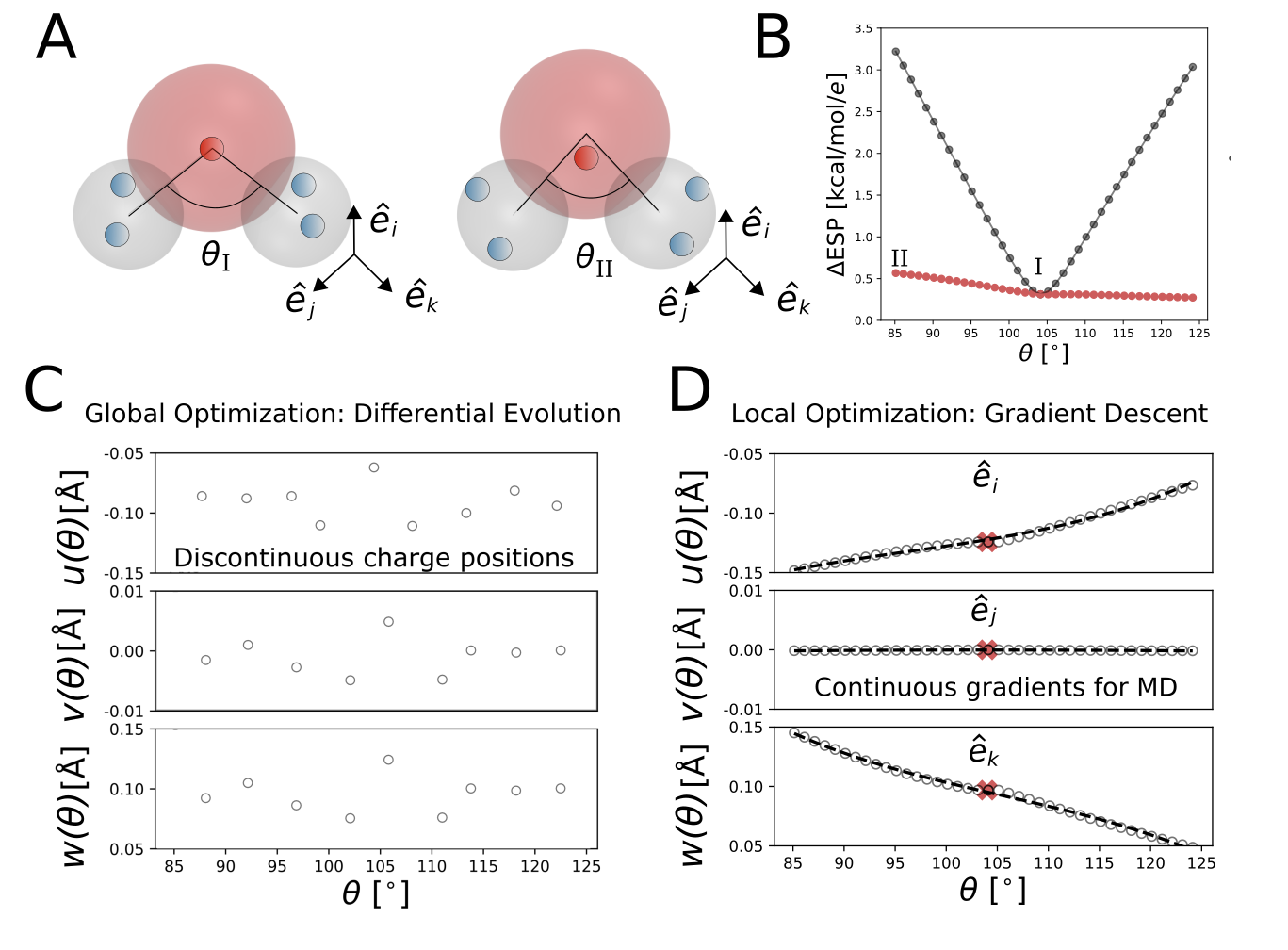
Figure 1: Panel A: Sketch of a 5-charge (small red and blue spheres) MDCM model for the equilibrium structure of water (structure I with $\theta_{\rm I}$; large red sphere for oxygen, large grey spheres for hydrogens) and for a perturbed structure (structure II with $\theta_{\rm II}$). Between structures I and II, the distributed charge positions adapt. Panel B: quality of the ESP from conventional MDCM optimized on the minimum energy structure and applied to perturbed structures along $\theta$ for water (black circles) and for fMDCM using the MDCM model for the minimum energy structure as the reference (red circles). Structures I and II are labelled. Panel C: Independent fitting of optimal MDCM charges using differential evolution leads to discontinuous charge positions ($u(\theta)$, $v(\theta)$, and $w(\theta)$) as a function of geometry. Panel D: Using gradient descent, starting from the equilibrium conformation (red cross) yields continuous charge displacements $u(\theta)$, $v(\theta)$, and $w(\theta)$. The vectors $\hat{e}_{{\alpha}}$ $(\alpha=i,j,k)$ define the local axes.

2.2 Flexible Distributed Charge Model (fMDCM)

Charge redistribution in fMDCM is captured by introducing a molecular geometry-dependent position of the off-centered charges, see change in positions of small blue spheres depending on $\theta$ in Figure 1A. In the current example a model is developed for $\theta-$dependent positions of the MDCM charges which leads to a flexible MDCM (fMDCM) model in which the magnitudes of the off-centered charges are invariant but their position relative to the nucleus can vary.

First, an MDCM charge model of a given order is developed for a reference geometry which is the equilibrium geometry for all 4 molecules considered. These reference models for water, formic acid, formamide and dimethylether used 6, 12, 17 and 13 charges, respectively, which offer a good compromise between accuracy and computational expense. The positions of the MDCM charges are defined uniquely relative to a set of local reference frames that are invariant to molecular translation and rotation, and approximately retain the charge positions relative to selected neighboring atoms upon conformational change.¹⁴ The reference MDCM model is determined by minimizing

$$\Delta{\rm ESP}=\sqrt{\frac{1}{N}\sum_{i=1}^{N}(V({\bf r}_{i})-V^{\rm{ref}}({\bf r}_{i}))^{2}}$$ (1)

where $N$ is the number of ESP grid points used for fitting, typically $\sim 10^{4}$ to $10^{5}$ and specifically 25000 points for water. $V({\bf r}_{i})$ is the ESP at grid point ${\bf r}_{i}$ generated by the point charge model and $V^{\rm ref}({\bf r}_{i})$ is the DFT reference value. Differential evolution (DE)²⁷ was used to identify a minimal set of charges at off-nuclear sites that accurately describe the ESP around a molecule, typically with an accuracy similar to that of a multipole expansion truncated at quadrupole or higher.¹⁵ Symmetry constraints were applied during fitting to ensure that the fitted charge distributions have the same symmetry as the parent molecule.

If independent MDCM models are determined for the $\theta-$perturbed structures, the MDCM charge positions vary in a non-continuous fashion due to the stochastic nature of DE, see Figure 1C. This complicates the interpolation of charge displacements for $\theta-$values between grid points and also affects the accuracy of the associated forces. For conceiving a model with smoothly varying charge positions as the internal coordinates change, gradient descent $\mathbf{\chi}_{n+1}=\mathbf{\chi}_{n}-\eta\nabla F(\mathbf{\chi}_{n})$ was used, where $\mathbf{\chi}$ is the vector of charge positions in the global reference (i.e. $x$, $y$ and $z$) and $\nabla F(\mathbf{\chi})$ is the gradient of the RMSE in Eq. 1 with respect to a change in charge position. A constant scaling factor $\eta=0.5$ Ų (kcal/mol/$e$)^-1 was used to limit the step size in the gradient descent optimization. The gradient was determined numerically by finite-difference with a step size of $0.2$ Å. This combination of step size and scaling factor was found to be appropriate and led to smooth, continuous displacements of the fMDCM charges as the geometry of the molecule changes, see Figure 1C. The sensitivity of $\Delta$ESP with respect to the number of grid points used to represent the ESP cube was found to converge to the same error as a fine grid ($6.67$ points/Å) at a grid spacing of $1.67$ points/Å. Due to the significant decrease in computational costs, this grid spacing was used throughout this study unless mentioned otherwise.

As an additional improvement of MDCM itself, conformationally averaged MDCMs were fitted to multiple conformers by generating a new ESP reference grid for each conformer, and then transforming each candidate charge model using its local axes to generate an associated trial ESP during DE.

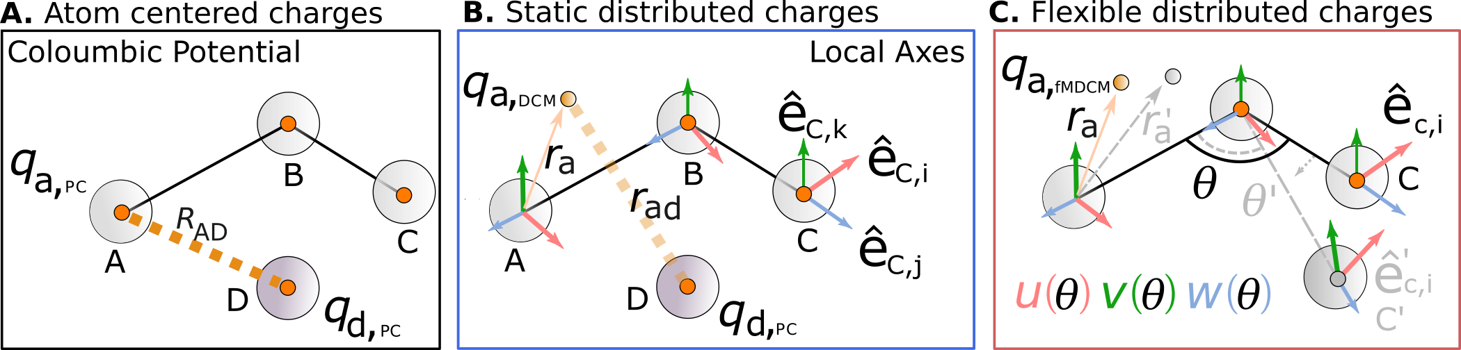
Figure 2: Panel A. The Coulombic interaction and its derivative are proportional to the distance between nuclear centers in atom centered point charge models. Panel B. In MDCM, this distance changes as charges are shifted from nuclear positions within the local frame, $\hat{\bf e}$, of three reference axes depicted by the red, blue, and green. Panel C. Charge positions within the local frame of the fMDCM model also depend on the angle $\theta_{\mathrm{ABC}}$. Parametrized functions $u(\theta)$, $v(\theta)$, $w(\theta)$ describe distances along each local axis. Variable names set in grey (i.e. $r_{a}^{\prime}$, $\theta^{\prime}$, etc.) show how an fMDCM charge responds upon changing $\theta$, requiring a modified derivative of the Coulombic potential for energy conserving forces in fMDCM.

For MD simulations the derivatives of the interactions with respect to the Cartesian coordinates of the nuclei are required. To derive the necessary expressions, the situation in Figure 2 is considered. Omitting the prefactor $(4\pi\varepsilon_{0})^{-1}$, the Coulomb potential between sites A and D for a conventional point charge (PC) model is $V\propto\frac{q_{\rm a,PC}\cdot q_{\rm d,PC}}{R_{\rm AD}}$, see Figure 2A. The derivative of the corresponding Coulomb potential with respect to some change in position of nucleus A, where $\alpha=(x,y,z)$, is then

$$\frac{\partial V}{\partial R_{{\rm A},\alpha}}=q_{\rm a,PC}\cdot q_{\rm d,PC}\frac{\partial}{\partial R_{{\rm A},\alpha}}\frac{1}{|{\bf r}_{\rm ad}|}$$ (2)

The situation is similar for distributed charges, but to allow conformational and rotational transformation of the molecule, ${\bf r}_{\rm a}$ is defined relative to a local axis system $\hat{\bf e}_{{\rm A,x}}$, $\hat{\bf e}_{{\rm A,y}}$, $\hat{\bf e}_{{\rm A,z}}$ defined by atoms $A$, $B$ and $C$, as described elsewhere.¹⁴ Forces on the off-center charge $q_{\rm a,DCM}$ of atom $A$ generate torques on $A$, $B$ and $C$ by re-evaluating equation (2) for these three atoms. The complete set of partial derivatives for charge $q_{\rm a,DCM}$ in Figure 2B is:

$$\frac{\partial V}{\partial R_{{\rm a},\alpha}} =\frac{-q_{\rm a,DCM}q_{\rm d,PC}\bigl{(}R_{{\rm AD},x}(\hat{\mathbf{\alpha}}\cdot\mathbf{\hat{x}}+g_{1\alpha})+R_{{\rm AD},y}(\hat{\mathbf{\alpha}}\cdot\mathbf{\hat{y}}+g_{2\alpha})+R_{{\rm AD},z}(\hat{\mathbf{\alpha}}\cdot\mathbf{\hat{z}}+g_{3\alpha})\bigr{)}}{r_{\rm AD}^{3}}$$ (3)

$$\frac{\partial V}{\partial R_{{\rm b},\alpha}} =-\frac{q_{\rm a,DCM}q_{\rm d,PC}(R_{{\rm AD},x}g_{4\alpha}+R_{{\rm AD},y}g_{5\alpha}+R_{{\rm AD},z}g_{6\alpha})}{r_{\rm AD}^{3}}$$ (4)

$$\frac{\partial V}{\partial R_{{\rm c},\alpha}} =-\frac{q_{\rm a,DCM}q_{\rm d,PC}(R_{{\rm AD},x}g_{7\alpha}+R_{{\rm AD},y}g_{8\alpha}+R_{{\rm AD},z}g_{9\alpha})}{r_{\rm AD}^{3}}$$ (5)

where the scalar product $\hat{\mathbf{\alpha}}\cdot\mathbf{\hat{x}}$ is 1 for $\alpha=x$ and zero otherwise. $R_{{\rm AD},x}$ is the $x$-component of the vector $\mathbf{R}_{\rm AD}$ from nucleus A to nucleus D. The coefficients $g_{1\alpha}$ to $g_{9\alpha}$ contain the partial derivatives of the local unit vectors of the frame ($\mathbf{\hat{e}}_{x},\mathbf{\hat{e}}_{y},\mathbf{\hat{e}}_{z}$) with respect to the nuclear coordinates $R_{{\rm a},\alpha}$, $R_{{\rm b},\alpha}$ and $R_{{\rm c},\alpha}$. In MDCM the local charge position is independent of $\theta$. The coefficient for the partial derivatives of frame $\mathbf{\hat{e}}_{x}$ with respect to atom A, for example, is

$$g_{1\alpha} =u\frac{\partial\mathbf{\hat{e}}_{x,i}}{\partial R_{{\rm a},\alpha}}+v\frac{\partial\mathbf{\hat{e}}_{y,i}}{\partial R_{{\rm a},\alpha}}+w\frac{\partial\mathbf{\hat{e}}_{z,i}}{\partial R_{{\rm a},\alpha}}$$ (6)

The prefactors $u$, $v$, and $w$ describe the position of the charge in the local reference axis system and the remaining coefficients $g_{2\alpha}$ to $g_{9\alpha}$ have been explicitly given in previous work.¹⁴

If atom “A” is treated with a fMDCM model, see Figure 2C, the potential changes to $V\propto\frac{q_{\rm a,fMDCM}\cdot q_{\rm d,PC}}{r_{\rm ad}}$ where $r_{\rm ad}$ depends on the A-B-C angle $\theta$ because the position ${\bf r}_{\rm a}$ of the fMDCM charge is defined as a function of $\theta$. This adds a $\theta-$dependence to the vector ${\bf r}_{\rm ad}=({\bf r}_{\rm d}+{\bf R}_{\rm D})-({\bf r}_{\rm a}+{\bf R}_{\rm A})$. Component $\alpha$ of ${\bf r}_{\rm a}$ is defined by the local axes according to

$$r_{{\rm a},\alpha}=u(\theta)\>{\bf\hat{e}}_{{\rm A,x},\alpha}+v(\theta)\>{\bf\hat{e}}_{{\rm A,y},\alpha}+w(\theta)\>{\bf\hat{e}}_{{\rm A,z},\alpha}$$ (7)

Here, $u(\theta)$, $v(\theta)$ and $w(\theta)$ are functions of the A-B-C angle $\theta$, and describe the distance along $\hat{\bf e}_{{\rm A,x}}$, $\hat{\bf e}_{{\rm A,y}}$, and $\hat{\bf e}_{{\rm A,z}}$, respectively.

As fMDCM charge positions are a function of $\theta$, additional terms enter the derivative for the force evaluations. The partial derivative, equation 6, becomes

$$g_{1\alpha}(\theta) =\Bigg{[}u(\theta)\frac{\partial\mathbf{\hat{e}}_{x,i}}{\partial R_{{\rm a},\alpha}}+\mathbf{\hat{e}}_{x,i}\frac{\partial u(\theta)}{\partial R_{a,x}}\Bigg{]}+\Bigg{[}v(\theta)\frac{\partial\mathbf{\hat{e}}_{y,i}}{\partial R_{{\rm a},\alpha}}+\mathbf{\hat{e}}_{y,i}\frac{\partial v(\theta)}{\partial R_{a,x}}\Bigg{]}+\Bigg{[}w(\theta)\frac{\partial\mathbf{\hat{e}}_{z,i}}{\partial R_{{\rm a},\alpha}}+\mathbf{\hat{e}}_{z,i}\frac{\partial w(\theta)}{\partial R_{a,x}}\Bigg{]}$$ (8)

whereby $u(\theta)$, $v(\theta)$ and $w(\theta)$ can be any suitably parametrized function or numerically defined by using, e.g., a reproducing kernel.²⁸ In the present work a cubic polynomial $u(\theta)=k_{1}+k_{2}\theta+k_{3}\theta^{2}+k_{4}\theta^{3}$ was used. The change in local coordinate versus nuclear position is, for example, $\frac{\partial u(\theta)}{\partial\theta}\frac{\partial\theta}{\partial R_{a,x}}$. More generally, $u({\bm{\rho}})$, $v({\bm{\rho}})$ and $w({\bm{\rho}})$ can be functions of any subset ${\bm{\rho}}$ of internal coordinates within a molecule that describe the conformation, such as 4 atoms describing a torsion or larger sets of atoms describing multiple degrees of freedom. In this case, the set of partial derivatives is simply extended to also include these atoms.

The energy and force expressions were implemented in CHARMM version c47, and simulations for several test systems were carried out to illustrate their use, and to verify energy conservation in $NVE$ simulations. The angular dependent terms and associated derivatives for fMDCM presented here need to be evaluated for each charge at each simulation time step. This incurs a computational cost which scales linearly with the number $N$ of charges in the system. For DCM¹⁴ and the same number of charges as for a fixed point charge model the computational overhead was a factor of $\sim 2$ which, however, has been further reduced in the meantime due to improvements in the code. As the system size increases, the dominating factor becomes the charge-charge Coulomb interactions that scale $\propto N\log N$ and the relative increase in compute time between fMDCM and PCs with the same $N$ will be considerably smaller than 2. The present implementation of fMDCM also supports parallelization with MPI and as will be shown below, multi-nanosecond simulations for water boxes are readily possible.

2.3 Molecular Dynamics Simulations

A first set of test simulations included one positively charged potassium ion surrounded by three water molecules described by fMDCM. The OH bond and HOH angle were flexible with force constants of $450$ kcal/mol/Ų and 55 kcal/mol/rad² for the stretching and bending motions, respectively, as available from CGenFF²⁹. These were used alongside the equilibrium bond distances and angles ($r_{e}=0.9572$ Å and $\theta_{e}=104.52^{\circ}$), nuclear charges and Lennard–Jones parameters from the TIP3P water model.³⁰ The simulations started from a distorted geometry of the cluster using a time step of $\Delta t=0.5$ fs and propagating $2\times 10^{6}$ time steps in the $NVE$ ensemble. The ion was used to avoid decomposition of the small water cluster.

Next, MD simulations with the fMDCM model for water were initiated from a snapshot of a water box containing $251$ water molecules, taking coordinates that were previously minimized with CHARMM TIP3P with SHAKE³¹ constraints, generated using the CHARMM GUI server.³² The same scheme and force field as for the previous $NVE$ simulations was used, with $\Delta t=0.5$ fs. These simulations employed periodic boundary conditions (PBC) and a $14$ and $12$ Å cut-off for electrostatics and VDW, respectively. Velocities were initially assigned from a Boltzmann distribution at $100$ K; however, no velocity rescaling was carried out during the $NVE$ simulations. Finally, heating, equilibration and $NVE$ production MD simulations with PBC were carried out at 300 K for rigid and flexible water molecules.

MD simulations were also used to generate structures of the test molecules to probe the performance of fMDCM models on more generally distorted structures than specifically scanning along one valence angle. For generating such perturbed structures for formic acid, formamide and dimethyl ether, the CGenFF²⁹ parametrization was used whereas for water the same parameters as previously described were employed. All test molecules were solvated in a $20$ ų TIP3P water box, equilibrated at $300$ K, with periodic boundary conditions, using the Nosé thermostat³³. All bonds to H-atoms were treated using SHAKE³¹, except for the flexible water simulations. Coordinates were saved every $200$ fs (formic acid, formamide, dimethyl ether) or $50$ fs (water). To select a diverse set of conformers to analyze further, principal component analysis (PCA), a dimensionality reduction technique, was performed as implemented in Scipy³⁴. PCA aids in interpreting the range of molecular conformations sampled, which are inherently high dimensional distributions. The projection was performed using a number of degrees of freedom, and the input was standardized by subtracting the mean and dividing by the standard deviation. Dihedral angles ($\phi$) are transformed by $|\sin{\phi}|$ to recover the isotropic distribution, before standardization and PCA. The $\Delta$ESP was calculated for these selected conformers, as described earlier.

3 Results

3.1 Quality of fMDCM

First, the quality of fMDCM is assessed by determining the accuracy with which the ESP from electronic structure calculations can be described for structures generated by scanning along an angle $\theta$ and a selected bond $r$. For water, formic acid, formamide, and dimethyl ether, the angles considered were the HOH, OCO, NCO, and COC angles, respectively, whereas the bonds investigated were the OH, C(sp²)O, CN, and CO (see Figure 3). Three charge models were explored for each of the four molecules: a conventional PC model fit to the ESP corresponding to the DFT optimized structure, a MDCM model optimized for the same structure, and the fMDCM model (as described in the methods section). PC models were fit to the same ESP grids as the MDCMs, but least-squares optimization was used in place of DE. The total charge of the molecule was constrained to zero. For reference, the $r-$ and $\theta-$ranges covered in finite-temperature ($300$ K) simulations for each of the compounds in solution are given as a histogram. The PC models (black symbols and lines) describe the ESP with typical RMSEs of between 1 and 2 kcal/mol/$e$ for angles (Figure 3A) and bonds (Figure 3B). The variation of the difference is within $\sim 0.5$ kcal/mol/$e$ except for scanning the OH bond in water and the CN bond in formamide for which the differences are larger.

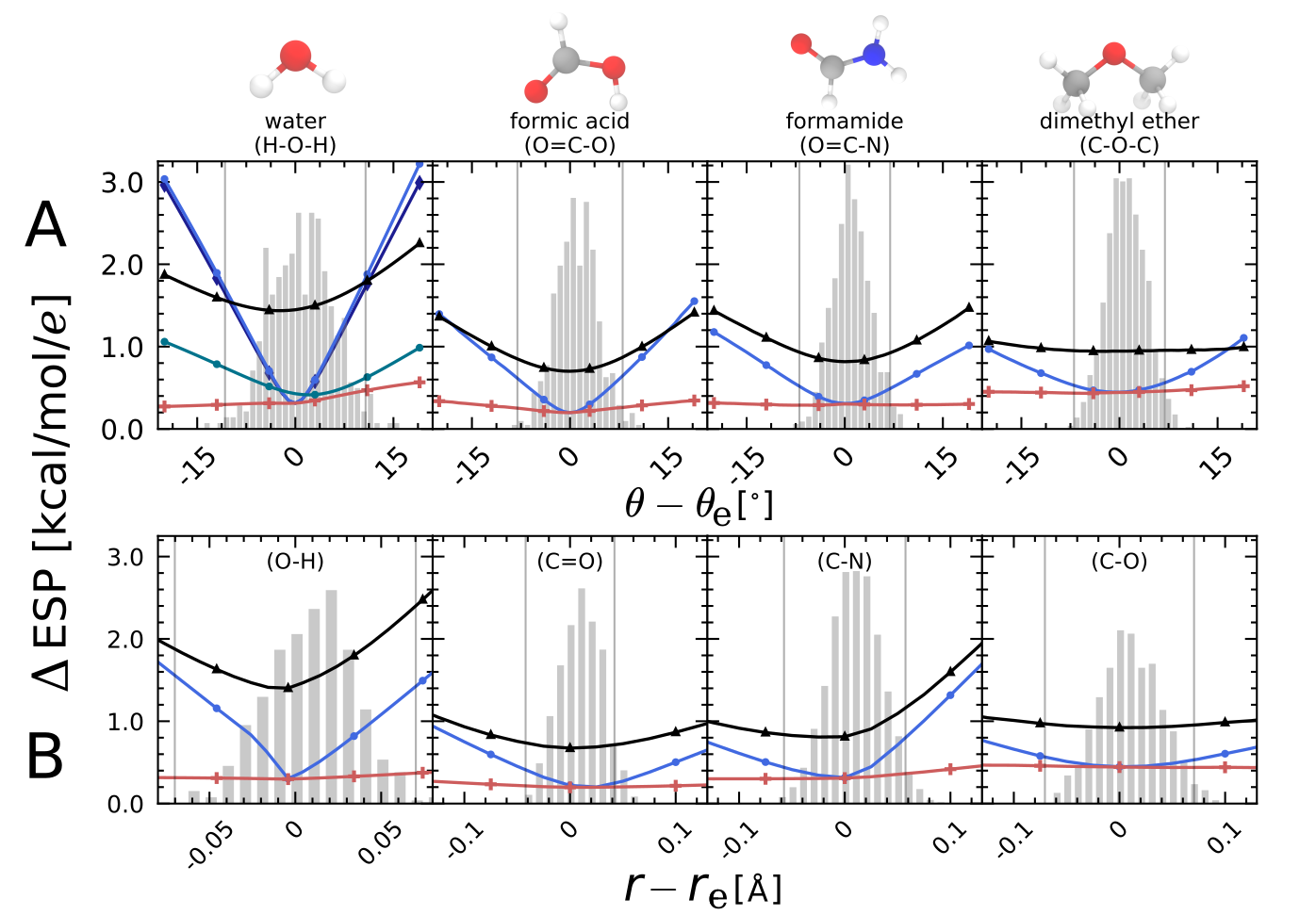
Figure 3: The angle (panel A) and bond length (panel B) dependence of the electrostatic potential from the DFT calculations and the fitted charge models for point charges (black) and the minimally distributed charge models with static (blue) and flexible (red) charges. The figure reports $\Delta{\rm ESP}$ as defined in Eq. 1. The MDCM models for water, formic acid, formamide, and dimethylether used 6, 12, 17 and 13 charges, respectively. The displacements $\theta-\theta_{\rm e}$ and $r-r_{e}$ are the displacements away from their respective equilibrium values $\theta_{\rm e}$. and $r_{\rm e}$. Grey histograms represent the approximate distributions of these angles which are thermally accessible at 300 K using point-charge molecular dynamics. In panel A for water the green line is the MDCM model fit to 3 structures and the dark blue line is for the “bisector definition” of the local reference axis system, see also Figure 4. The difference between fMDCM and the 3-conformation MDCM model represents the amount of charge flux accounted for in fMDCM but not captured in MDCM.

Compared with the PC model the best achievable model with MDCM (blue symbols and lines in Figure 3) is considerably better for all cases considered. All MDCM models reproduce the reference ESP for the minimum energy structures to within 0.2 to 0.4 kcal/mol/$e$ which is a factor of 3 to 5 times better than the best PC model. For perturbed structures along $\theta$ accessible at ambient conditions (grey histogram) the maximum RMSE of the MDCM model is comparable to that from the PC-based model as the rate at which the quality of the MDCM ESP deteriorates is more rapid when fitted to the equilibrium conformation only. Fitting to an expanded dataset of several conformers alleviates this problem, as demonstrated for water: this model was fitted to three different conformers (equilibrium structure and distorted geometries corresponding to the solid line in Figure 3A), leading to a more balanced model (green line) with similar performance for the equilibrium structure as the single-conformer MDCM, and similar behavior upon distortion to the PC model but with lower RMSE. The residual deterioration with conformational change can be attributed to the use of fixed charge positions, which do not capture charge redistribution. This result additionally supports previous findings that fitting multipolar charge models to multiple conformers separately, then averaging resulting multipole moments leads to more robust, transferable electrostatic models.³⁵ For distortions along the bond $r$ the changes are also more pronounced but remain below those from the PC models, see Figure 3B.

Finally, the flexible MDCM models (red symbols and lines) perform uniformly well. All RMSEs are below $\sim 0.5$ kcal/mol/$e$ across the geometry variations considered and for all cases considered - except for the scan along $\theta$ for water in Figure 3A - the difference with respect to the reference ESP is essentially flat. Hence, capturing the variation of positioning the MDCM charges while keeping their magnitude constant is a meaningful way to improve the description of the ESP as a function of internal geometry by a factor of 2 to 5 when compared with conventional atom-centered point charges.

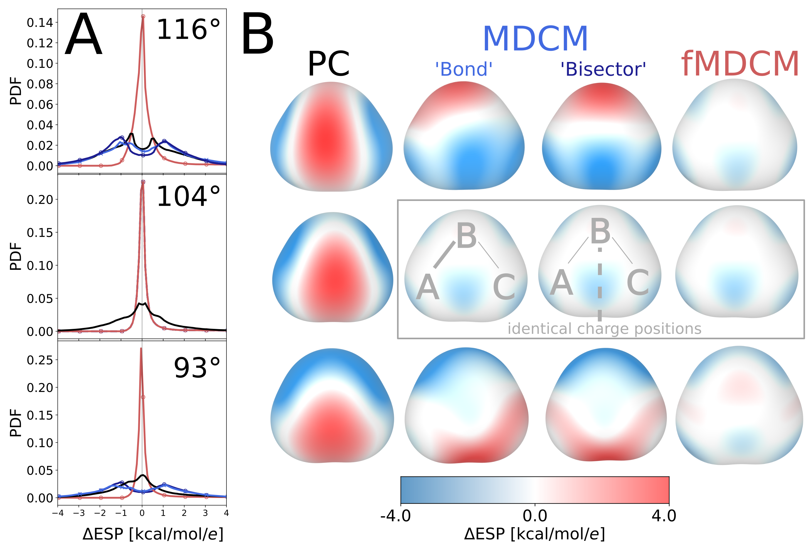
Figure 4: Panel A: The normalized error distributions between DFT ESP and ESP from the different charge models considered: point charges (black), MDCM “bond” (blue), “MDCM bisector” (dark blue) and flexible distributed charge models (fMDCMs, red) for three structures where $\theta={116^{\circ},104^{\circ},93^{\circ}}$. MDCM and fMDCM use 6 charges. Panel B: Error surfaces for all models and geometries. The defining bond (A-B) of the local reference system used for distributed charges is shown for the equilibrium MDCM surface. Using this bond as the local reference breaks the symmetry of the model creating uneven error distributions for the non-equilibrium MDCM models. When using a “bisector” model for MDCM the error distribution reflects molecular symmetry for all structures considered.

Next, the distribution of the RMSEs in the ESP incurred by adopting a PC, MDCM, and fMDCM representation for water is analyzed. This error analysis is carried out for DFT densities between $1.0\cdot 10^{-3}$ and $3.2\cdot 10^{-4}$ - representing the local electric field in regions relevant to MD simulation (Figure 4A) - and in terms of the location of these errors on the surface of the molecule at an isodensity value of $10^{-3}$ (Figure 4B). Conformers with angles of $116^{\circ}$, $104^{\circ}$, and $93^{\circ}$ were analyzed.

The normalized error distributions from the PC model fit to the equilibrium geometry extends out to $\sim\pm 4$ cal/mol/e, see Figure 4A (black line). The error projected onto the molecular 0.001 a.u. isodensity surface shows continuous regions of negative (blue) and positive (red) errors (Figure 4B). Near the oxygen atom the error surface is typically positive for protracted angles, and negative for contracted angles, as the magnitude and positions of the point charges remain constant with respect to nuclear position and hence do not adequately capture redistribution of the electron density. As the angle contracts, electron density (i.e. negative charge) moves from the oxygen atom down into the bisector of the two OH bonds - creating a region of positive error for the 93^∘ model. Similarly, acute distortions in the valence angle causes electron density to flow to the oxygen atom. Failure to account for this flow causes a region of positive error to form on the oxygen atom for the $116^{\circ}$ PC model. By construction, the point charge ESP is symmetric. The ab initio ESP is also symmetric, and it follows that the difference between the two is also symmetric as shown in Figure 4B.

For MDCM two models with different definitions of the local axes were generated for water. In the first model (“Bond”) the first axis points along the A-B bond, the second axis is orthogonal to the first axis and in the plane containing the three atoms and the third axis is orthogonal to the first and second axis. For such an axis system the error distribution is asymmetric (see Figure 4A) with respect to the molecular symmetry as the angle $\theta$ is perturbed away from the equilibrium geometry (see first and third row of column “Bond” in Figure 4B). On the other hand, for the equilibrium geometry, which was used for the MDCM fit, the error distribution is manifestly symmetric. If the local axis system uses the “bisector” (third row in Figure 4B) as has been used in previous work¹², the error distribution retains the symmetry of the molecular structure as also seen in Figure 4A. This highlights that the performance of a MDCM or multipolar electrostatic model upon geometry distortion can be affected by the choice of local axes, and while in certain cases a clear choice, such as tying an axis to a dominant bond or bisector, may be preferable,³⁶ in the general case of lower symmetry the choice is less clear. The figure also shows that the average error across all grid points is not typically strongly affected, however, as has already been observed in Figure 3A for water (dark vs. light blue lines).

The error distributions for fMDCM for all three structures are strongly peaked around zero, as is seen in Figure 4A (blue line). Also, fMDCM is more robust to the choice of local axes as charges are free to move back to more optimal positions than the local axes would have placed them upon distorting a molecule. The projected error distribution is also considerably more symmetric than for the corresponding MDCM model, despite using the generic “Bond” local axes. More importantly, using fMDCM greatly reduces the baseline error of the model, with the maximum of these distributions around $<\pm 1$ cal/mol/$e$ which is about a factor of 5 better than for the PC and MDCM models for the perturbed structures.

In summary, Figure 4B highlights the influence of capturing charge flow on the quality of the ESP determined from the different point charge-based representations. The particular choice of local reference axes can add an additional, but minor source of error for MDCM (or multipolar) models and fMDCM addresses both sources of errors to provide significant improvement across the entire range of distorted geometries.

3.2 Molecular Dynamics with fMDCM

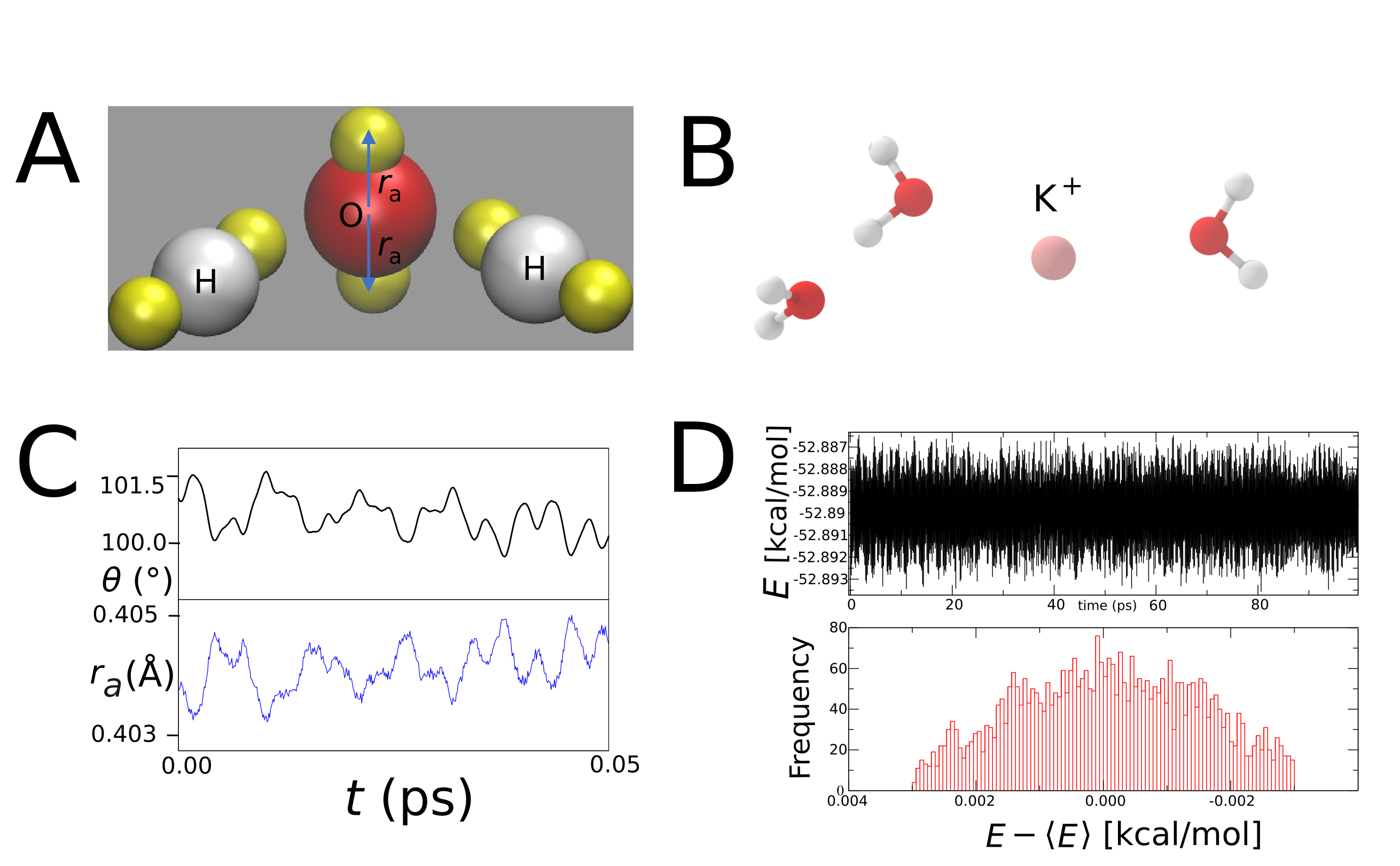
Figure S1: Panel A: The fMDCM water with the 6 off-center charges as yellow spheres and the oxygen and hydrogen atoms as red and white spheres, respectively, with $\theta$ as the HOH angle. Panel B: Explorative simulation system consisting of one potassium ion and three fMDCM water molecules. Panel C: Time series for angle $\theta(t)$ and the separation of one of the fluctuating charges with respect to the atom it is defined to, see panel A for definition of $r_{\rm a}$. Panel D: Time series for total energy $E(t)$ (top) and histogram for the fluctuation around the mean $P(E-<E>)$ (bottom) over 100 ps.

One particularly relevant application for conformationally dependent charges arises in dynamics studies of solvated compounds. The forces for MDCM and fMDCM can be determined in closed form and were implemented in CHARMM for carrying out such simulations. To validate the implementation, $NVE$ simulations were run for several systems of increasing complexity. First, three water molecules coordinated to one positively charged potassium ion in the gas phase were considered, see Figures S1A and B. This conveniently obviates the use of periodic boundary conditions for initial validation. This cluster was stable for the entirety of the simulation and the coordinates of the atoms and distributed charges were saved at every time step (1 fs). Unlike the standard MDCM implementation, the distance between each charge and the atom defining its local reference axis was flexible, changing smoothly in response to changes in the internal angle resulting in oscillating displacements of the charge as a function of time, see Figure S1C. Figure S1D reports the total energy $E(t)$ and its distribution $P(E)$ for these exploratory simulations.

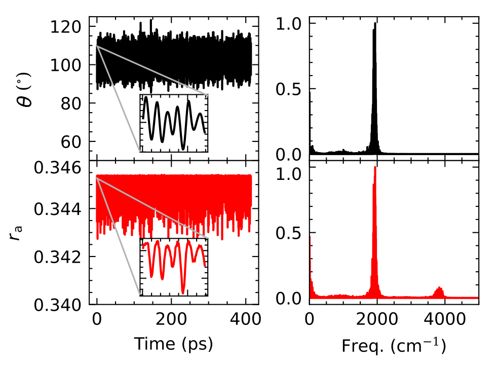
Figure S3: Correlation between valence angle $(\theta)$ and the distance between the reference atom (oxygen) and one of the associated conformationally flexible charges. The frequency spectrum obtained using the fast Fourier transform is also shown for the 400 ps trajectory. The simulation was heated and equilibrated to 300 K in the $NVT$ ensemble before dynamics were collected in the $NVE$ ensemble with $\Delta t=0.25$ fs.

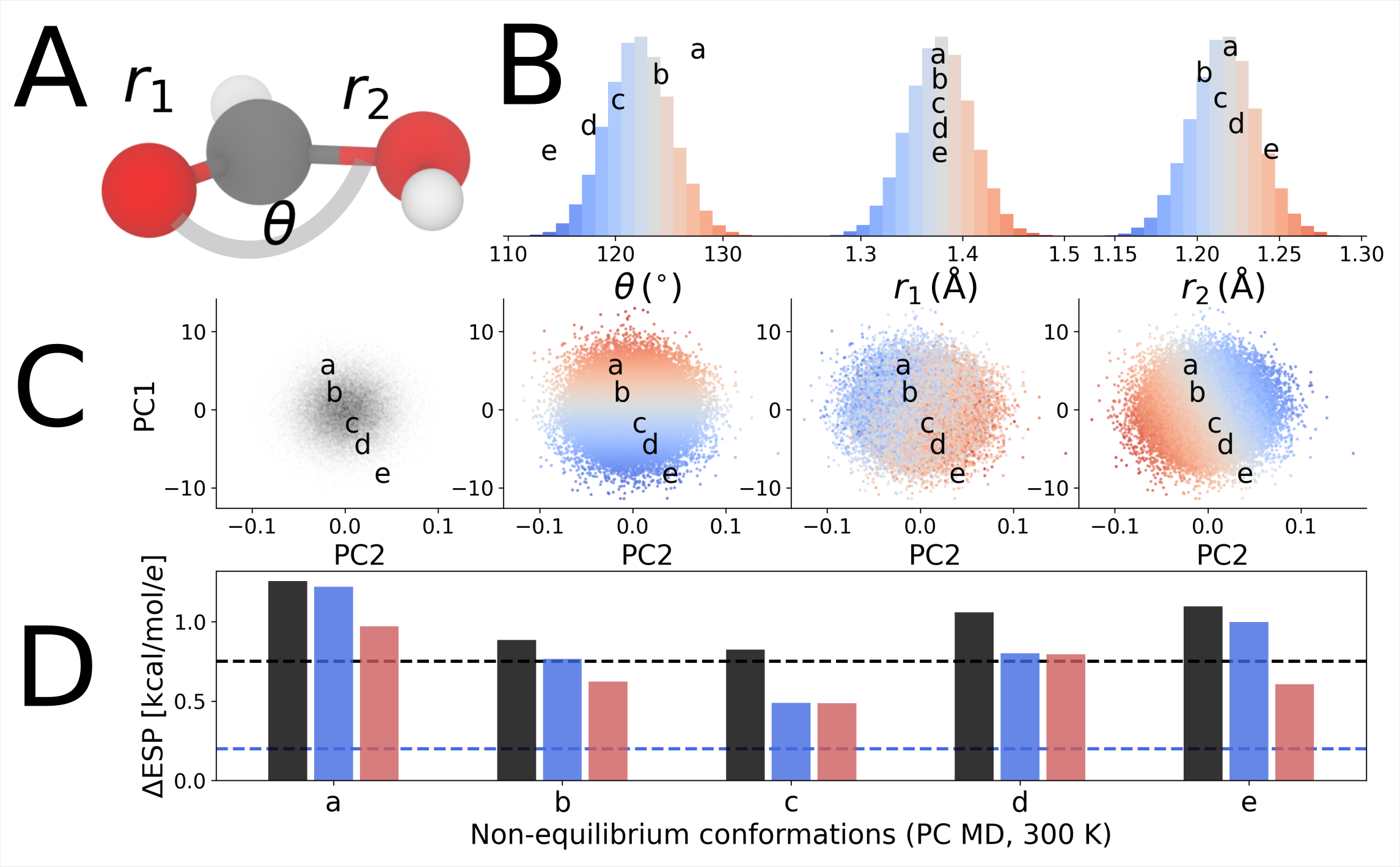
Figure S4: Performance of fMDCM for generally perturbed structures of formic acid. Panel A: Formic acid with relevant degrees of freedom ($r_{1}$, $r_{2}$ and $\theta$) shown explicitly. Panel B: 1D distribution of internal coordinates sampled from point charge (PC) SHAKE MD at 300 K. Panel C: 2D projection of these 3 degrees of freedom in principal component space. The red-gray-blue color scale indicates below-equilibrium, equilibrium, and above-equilibrium values, respectively. Panel D: RMSE for the ESP for non-equilibrium geometries, comparing PC (black), MDCM (blue) and fMDCM (red) fit to the valance angle. Dashed, blue and black horizontal lines indicate the quality of the equilibrium fit for PC and MDCM models, respectively.

A final validation and comparison between different methods was carried out for a simulation temperature of 300 K. Following heating (125 ps) and equilibration (125 ps) with periodic boundary conditions, a 10 ns $NVE$ simulation was run for flexible TIP3P, MDCM, and fMDCM. The energy fluctuation around the mean for all simulations are reported in Figures 5 and S2. For simulations with flexible bonds involving hydrogen atoms a shorter time step needs to be used. Here, $\Delta t=1$ fs was the time step for simulations with SHAKE and $\Delta t=0.25$ fs was used for simulations with flexible bonds involving hydrogen atoms. For a flexible water model and the PC, MDCM, and fMDCM models the width of the Gaussian distributed fluctuation around the mean is $\sim 0.2$ kcal/mol compared with $\sim 0.5$ kcal/mol for TIP3P with SHAKE. Total energy is manifestly conserved for all four simulations. In addition, it is of interest to consider the angle time series $\theta(t)$ and the corresponding distance between one of the 6 conformationally flexible, off-center charges relative to its defining atom $r_{a}(t)$, see Figure S3 (left column). The angle fluctuates by about $15^{\circ}$ around the equilibrium value whereas the charge fluctuates between 0.342 Å and 0.345 Å away from the atom it is defined to. The Fourier transform of the two time series (Figure S3, left column) establishes that one mode is related to the water bending mode (2000 cm^-1) together with low-frequency motions (probably due to water-water-water bending) and the bending overtone at about twice the fundamental frequency are present. For the same simulations with a time step of $\Delta t=1$ fs total energy is also conserved for all models considered, see Figure S4.

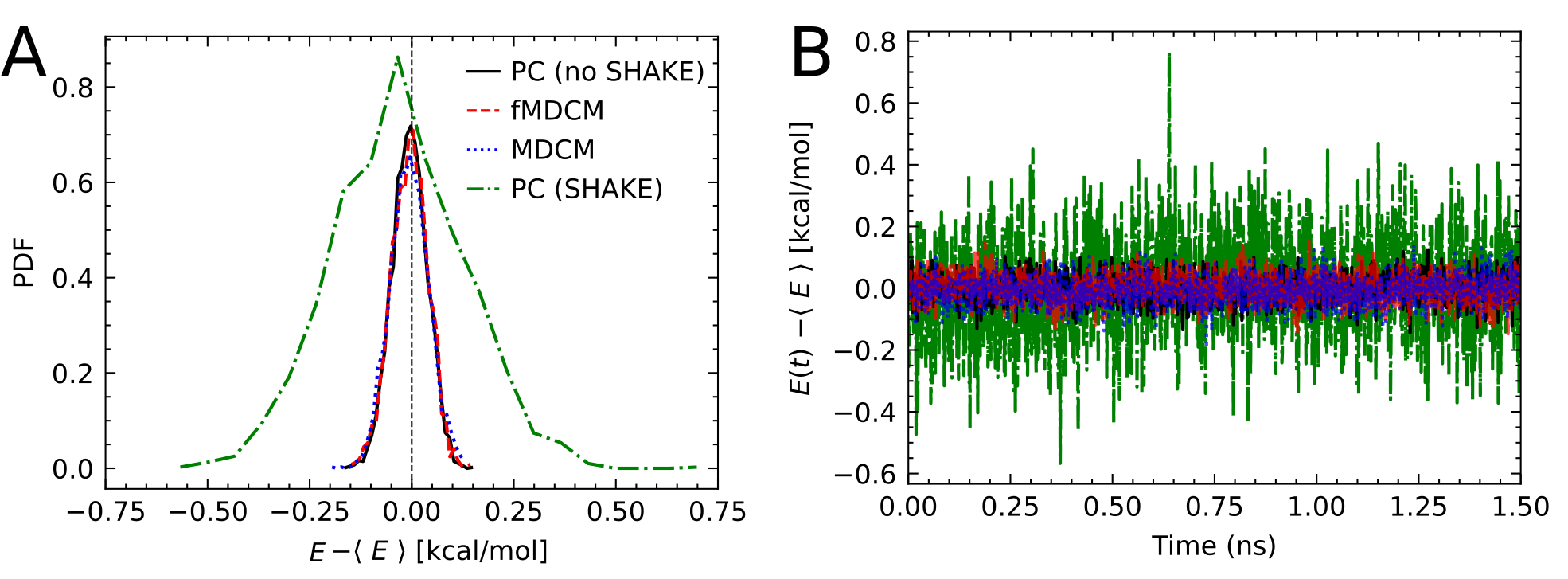
Figure 5: Distribution of energy fluctuations (panel A) and total energy time series (panel B) from 1.5 ns simulations at 300 K performed with TIP3P (with SHAKE, $\Delta t=1$ fs, green), TIP3P (flexible, $\Delta t=0.25$ fs, black), MDCM (flexible, $\Delta t=0.25$ fs, red), and fMDCM (flexible, and $\Delta t=0.25$ fs, blue). In all simulations total energy is well conserved and the distribution of the fluctuation around the mean is approximately Gaussian.

3.3 General Molecular Deformations

As a proof of concept the fMDCMs presented so far were fitted to accurately describe the ESP upon distortion of a single angle, see Figure 3. The following analyses were geared towards establishing whether such a model is also suitable to improve the description of the ESP when more general deformations of the molecules are allowed, including degrees of freedom that were not accounted for during fitting.

The necessary conformations were generated from MD simulations of the hydrated test molecules which were run at 300 K. Since the molecular geometry and ESP depends on $3n$ degrees of freedom, dimensionality reduction is used to project this space onto a 2D representation. This is done using principal components (PC1 and PC2), which maximize the explained variance of the original distribution. The frequency of the observed MD conformations is proportional to their energy; the peak of the principal component distribution, centered at the origins in these projections, corresponds to the equilibrium MD conformer.

To probe the performance of the model for arbitrarily perturbed structures, two molecules (formic acid and formamide) were considered. Based on the results of the relaxed scans in Figure 3, formic acid appears to be less sensitive to internal distortions than formamide. Additionally, formic acid requires fewer internal degrees of freedom to describe its conformation compared to formamide. To provide an impression of the performance of the model, formic acid structures were sampled from the parametrized range of $\theta$, while also sampling a range of $r_{2}$ bond lengths that were not part of the parametrization for fMDCM. Formamide conformers were sampled from the full range of internal angles and dihedrals to more widely probe the performance of each model across the available conformational space. The number of selected distorted structures was kept small (5 for each molecule) for clarity and are intended to provide guidance as for what regions of conformational space the model should, and should not, be trusted.

Five formic acid conformations (a to e) sampled from a simulation in water were analyzed (Figure S4). To set the stage, conformations were selected from the pool of structures such that $r_{1}$ was near the equilibrium value and only changes along $\theta$ and $r_{2}$ occurred. As suggested by the 2D distribution in principal component space, Figure S4C, structures a and e are sampled from the tails of this distribution. For all 5 structures considered the fMDCM model performs best (Figure S4D, red bar), followed by MDCM (blue) and PC (black). However, the deterioration compared with the performance on the reference structure (dashed horizontal line) is smallest for the PC model and largest for fMDCM. Compared with MDCM, the fMDCM model performs better or on par with it. In other words, the additional boost in accuracy obtained with fMDCM fitted to a single degree of freedom in this case also leads to somewhat improved performance for conformers with more general distortions that are far from the equilibrium conformation and involve other degrees of freedom, but performance is degraded.

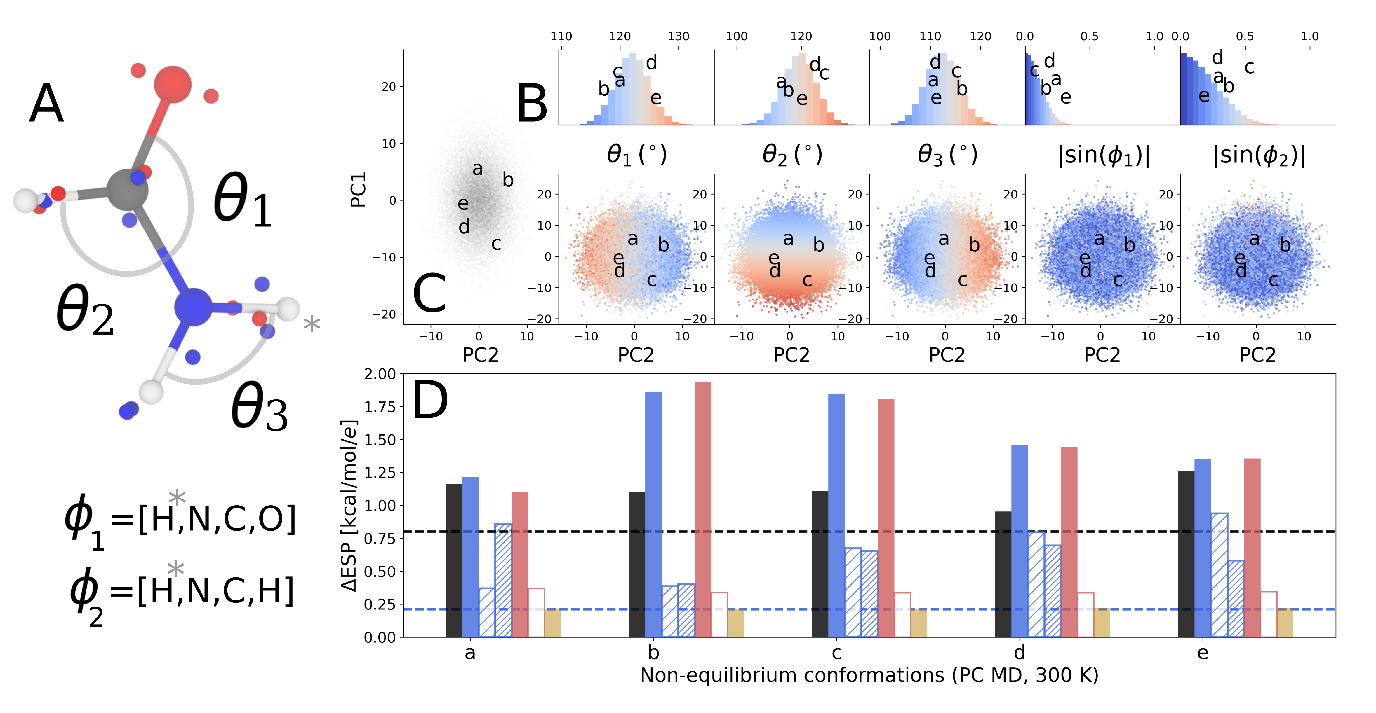
Figure 6: Performance of fMDCM for generally perturbed structures of formamide. Panel A: Formamide with 5 select degrees of freedom defined. MDCM charges are depicted as red and blue spheres. Panel B: 1D distribution of internal coordinates sampled from point charge (PC) MD at 300 K. The red-gray-blue color scale indicates below-equilibrium, equilibrium, and above-equilibrium values, respectively. Panel C: 2D projection of these 5 degrees of freedom in principal component space. Color scales are consistent with the 1D distributions above. Panel D: RMSEs in the ESP for non-equilibrium geometries a to e, comparing PC (black), MDCM (blue), fMDCM for the minimum energy structure (solid red), fMDCM for conformers a and b (light hatch), fMDCM fit to all five conformers a to e (thick hatch), fMDCM for each conformer a to e separately (empty red bar), and the 32-pole fit (gold). Dashed, blue and black horizontal lines indicate the quality of the equilibrium fit for PC and MDCM models, respectively.

As a second example formamide was considered to probe the quality outside the parametrized regime, see Figure 6A. The degrees of freedom considered are angles $\theta_{1}$ to $\theta_{3}$ and dihedrals representing the rotation around the CN bond, $\phi_{1}$ and $\phi_{2}$. The bond lengths involving hydrogen atoms were SHAKEd in the simulations. Hence, with respect to the DFT equilibrium structures, the bond lengths are distorted in the samples analyzed.

As for formic acid, five formamide conformers from the MD simulations were extracted by selecting geometries with non-equilibrium values of all degrees of freedom (except for bonds involving hydrogen atoms, see above) in the tails of the probability distributions (Figures 6B and C). The ESP from the PC model (black bars in Figure 6D) differs from the ESP for the minimum energy structure for which it had been fitted by $\sim 30$ % and the RMSE is quite uniform across the five selected structures. This is different for the MDCM (blue bar) and fMDCM (red bar) models. For those, the RMSE varies less uniformly and is larger by a factor of 6 to 10 compared with the structure for which they were parametrized (blue dashed horizontal line). The RMSE can be reduced to comparable levels as for the reference structure if the MDCM model is optimized for each of the five structures individually (red open bar) and compares favourably with a full optimization at the 32-pole level (gold), suggesting what could be achieved by an fMDCM that depends on all degrees of freedom simultaneously. This confirms the findings for point charges as a model that is generally transferable and for formamide reproduces the ESP uniformly with an accuracy of $\sim 1$ kcal/mol across various conformations. For MDCM it is also confirmed that the performance can deteriorate for deformations further away from the reference conformation and for fMDCM if deformations include regions for which the model was not parametrized.

As a final comparison, it was investigated to what extent conformational averaging, as had already been done for water, see Figure 3A, could reduce sensitivity to conformational change for formamide - in other words: to what extent transferability across geometric changes could be retained. Explicitly including ESP grids of conformers a to e (red hatched bars in Figure 6D) during DE fitting results in an MDCM model that is on par or evidently better than PC or MDCMs that do not include such conformational information. Including the 2 conformers a and b during fitting leads to a marked improvement of the resulting MDCM when predicting ESP grids for conformers c to e (see light blue hatch in 6D), despite their relative distance in conformational space. This suggests that it is not necessary to widely sample conformational space in order to improve conformational sensitivity and transferability of MDCMs. If all five conformers a to e are included (thick blue hatch in 6D), the overall performance of MDCM is greatly improved compared with MDCM fit to a single conformer although except for conformer a, for which the RMSE is only slightly reduced. An optimal balance in performance can therefore be achieved by including relevant conformers when fitting ESP-derived charge models, while significant improvement can already be obtained by using at least two conformers in order to discard charge models that are excessively sensitive to conformational change. In addition, while explicit inclusion of all degrees of freedom when parametrizing an fMDCM will yield the best results, fitting the fMDCM from a conformationally-averaged MDCM starting point should also reduce the performance degradation when sampling conformational space outside the parametrized range.

4 Discussion and Conclusion

Distributed charge models are a computationally efficient way to improve the description of the molecular ESP which is essential to capture when evaluating electrostatic interactions in quantitative atomistic simulations. This work demonstrates that a continuous description for off-center point charges can be obtained using gradient descent that recovers the conformational dependence of the reference ESP. The model also yields analytical derivatives with respect to atom positions that allow energy conserving MD simulations and the implementation in the CHARMM simulation package was validated for water treated with periodic boundary conditions.

For models trained on a single reference structure it is found that conventional point charges fitted to the ESP have an almost uniform RMSE (1 to 2 kcal/mol/$e$ for the molecules considered here) for deformations away from the reference structure. This is different for MDCM and fMDCM models. For MDCM the RMSE on the fitted structure is typically lower by a factor of 2 to 5 but increases rapidly for deformations away from the reference structure. This is much improved in the case of fMDCM for which the RMSEs remain small for perturbations along degrees of freedom for which the model was parametrized. If, however, perturbations of the structures outside the range or orthogonal to the degrees of freedom for which they were parametrized occur, the performance can deteriorate appreciably and even become worse than for a PC-based model. One remedy to this, explored in the present work, is to develop MDCM models by fitting to the ESPs of a range of conformers without significant degradation of the quality of the model of each conformer. Models that are too sensitive to conformational distortion are thereby discarded during fitting. Flexible MDCM again offers a robust alternative, however, by explicitly relaxing charge positions to resolve unfavorable distortions, but only if all relevant degrees of freedom that describe the conformational change are accounted for by the model. A future extension of the fMDCM framework introduced here is to generalize parametrization of the $u({\bm{\rho}})$, $v({\bm{\rho}})$ and $w({\bm{\rho}})$ to additional internal degrees of freedom for which machine learning techniques offer interesting possibilities.

The correct description of the ESP with changing molecular geometry also yields fluctuating molecular dipole moments which can be advantageous in spectroscopic applications. This has, for example, been demonstrated from simulations of H₂CO with the PhysNet model.³⁷ PhysNet³⁸ is trained on energies, forces, and partial charges for a set of nuclear configurations and therefore includes (atom centered) charge variation depending on geometry. It was found that for H₂CO the relative intensities of the vibrational bands agree very well with those observed from experiments. Thus, it will be of interest to use fMDCM for spectroscopic applications. In addition, the formulation of the fMDCM model is ideally suited to also incorporate effects of external polarization. Methods such as the Drude or the “charge on a spring” model already use off-center charges to capture polarization. Incorporating external polarization in fMDCM will amount to additional slight repositioning of a subset of charges in response to the external electrical field.

In addition to charge redistribution, the local axis system used is found to slightly impact on the error distribution for the ESP upon conformational change for MDCM. While such issues can be partially addressed by careful choice of local axes, fMDCM offers a robust alternative as charge positions are allowed to drift to compensate for changes in the direction of local axes upon conformational change.

From the broader perspective of force field development the fMDCM model provides a starting point for treating nonbonded interactions at a similar level as compared with kernel- or neural network-based methods for bonded interactions.^{39, 40} It has been shown for small molecules that the potential energy surface of a molecule can be described with exquisite accuracy (${\rm RMSE}\sim 10^{-2}$ to $10^{-3}$ kcal/mol) from using reproducing kernel Hilbert space^{37, 41} or permutationally invariant polynomials.⁴² Therefore, combining such ML-based models for the bonded interactions with fMDCM (and polarizable fMDCM) is expected to be a powerful extension for condensed-phase simulations. The remaining term for a comprehensive description of the inter- and intramolecular interactions, not accounted for so far, are the van der Waals contributions.

In conclusion, for the molecules considered here fMDCM is capable of describing the reference ESP of conformationally distorted structures on average better by a factor of $\sim 5$ compared with PC and MDCM while correctly capturing effects of charge rearrangement due to changes in the molecular geometry. The formulation of a distributed, flexible point charge-based model presented here generalizes to larger molecules including deformations along all internal degrees of freedom. For this, the functions $u({\bm{\rho}})$, $v({\bm{\rho}})$ and $w({\bm{\rho}})$ need to be represented either as parametrized expressions or, probably more conveniently, be learned using a ML-based technique such as a neural network or a reproducing kernel.

This work was supported by the Swiss National Science Foundation through grant 200020-188724, the NCCR MUST, and the University of Basel (to MM).

SUPPORTING INFORMATION:Molecular Dynamics with Conformationally Dependent, Distributed Charges

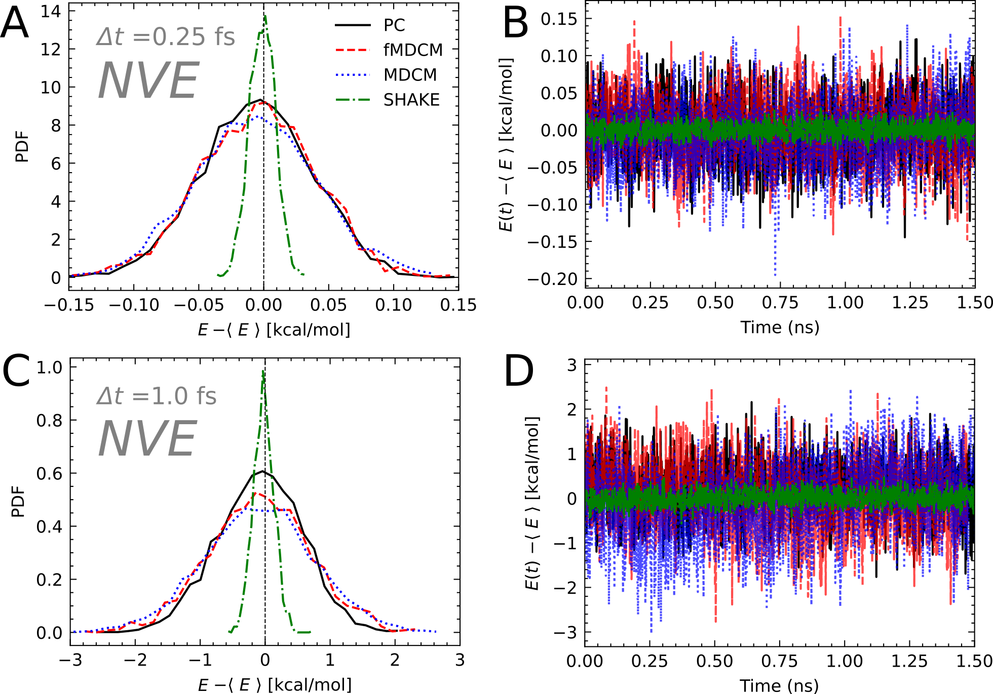
Figure S2: Distribution of energy fluctuations and time series for simulations performed at an integration time step of 0.25 fs (panels A and B) and 1 fs (panels C and D). Even with flexible water for the three electrostatic models total energy is conserved for simulations with 1 fs time step and the distribution of the energy around the mean is Gaussian. Note the different axes ranges for $E-<E>$ in panels A/B vs. C/D.

References

- Auffinger et al. 2004 Auffinger, P.; Hays, F. A.; Westhof, E.; Ho, P. S. Halogen bonds in biological molecules. Proc. Natl. Acad. Sci. USA 2004, 101, 16789–16794
- Lommerse et al. 1996 Lommerse, J. P. M.; Stone, A. J.; Taylor, R.; Allen, F. H. The Nature and Geometry of Intermolecular Interactions between Halogens and Oxygen or Nitrogen. J. Am. Chem. Soc. 1996, 118, 3108–3116
- Hardegger et al. 2011 Hardegger, L. A.; Kuhn, B.; Spinnler, B.; Anselm, L.; Ecabert, R.; Stihle, M.; Gsell, B.; Thoma, R.; Diez, J.; Benz, J.; Plancher, J.-M.; Hartmann, G.; Banner, D. W.; Haap, W.; Diederich, F. Systematic Investigation of Halogen Bonding in Protein–Ligand Interactions. Angew. Chem. Int. Ed. 2011, 50, 314–318
- Politzer et al. 1985 Politzer, P.; Laurence, P. R.; Jayasuriya, K. Molecular Electrostatic Potentials: An Effective Tool for the Elucidation of Biochemical Phenomena. Environ. Health Perspect. 1985, 61, 191–202
- Kukić and Nielsen 2010 Kukić, P.; Nielsen, J. E. Electrostatics in proteins and protein–ligand complexes. Future Med. Chem. 2010, 2, 647–666
- Castner Jr et al. 2011 Castner Jr, E. W.; Margulis, C. J.; Maroncelli, M.; Wishart, J. F. Ionic Liquids: Structure and Photochemical Reactions. Annu. Rev. Phys. Chem. 2011, 62, 85–105
- MacKerell, Jr. et al. 1998 MacKerell, Jr., A. D. et al. All-atom empirical potential for molecular modeling and dynamics studies of proteins. J. Phys. Chem. B 1998, 102, 3586–3616
- Christen et al. 2005 Christen, M.; Hünenberger, P. H.; Bakowies, D.; Baron, R.; Bürgi, R.; Geerke, D. P.; Heinz, T. N.; Kastenholz, M. A.; Kräutler, V.; Oostenbrink, C.; Peter, C.; Trzesniak, D.; van Gunsteren, W. F. The GROMOS software for biomolecular simulation: GROMOS05. J. Comput. Chem. 2005, 26, 1719–1751
- Case et al. 2005 Case, D. A.; Cheatham, T. E.; Darden, T.; Gohlke, H.; Luo, R.; Merz, K. M.; Onufriev, A.; Simmerling, C.; Wang, B.; Woods, R. J. The Amber biomolecular simulation programs. J. Comput. Chem. 2005, 26, 1668–1688
- Lagardère et al. 2017 Lagardère, L.; El-Khoury, L.; Naseem-Khan, S.; Aviat, F.; Gresh, N.; Piquemal, J.-P. Towards scalable and accurate molecular dynamics using the SIBFA polarizable force field. AIP Conf. Proc 2017, 1906, 030018
- Popelier 2015 Popelier, P. QCTFF: on the construction of a novel protein force field. Int. J. Quantum Chem. 2015, 115, 1005–1011
- Ponder et al. 2010 Ponder, J. W.; Wu, C.; Ren, P.; Pande, V. S.; Chodera, J. D.; Schnieders, M. J.; Haque, I.; Mobley, D. L.; Lambrecht, D. S.; DiStasio Jr, R. A.; Head-Gordon, M.; Clark, G. N. I.; Johnson, M. E.; Head-Gordon, T. Current status of the AMOEBA polarizable force field. J. Phys. Chem. B 2010, 114, 2549–2564
- Devereux et al. 2009 Devereux, M.; Plattner, N.; Meuwly, M. Application of Multipolar Charge Models and Molecular Dynamics Simulations to Study Stark Shifts in Inhomogeneous Electric Fields. J. Phys. Chem. A 2009, 113, 13199–13209
- Devereux et al. 2014 Devereux, M.; Raghunathan, S.; Fedorov, D. G.; Meuwly, M. A Novel, computationally efficient multipolar model employing distributed charges for molecular dynamics simulations. J. Chem. Theory Comput. 2014, 10, 4229–4241
- Unke et al. 2017 Unke, O. T.; Devereux, M.; Meuwly, M. Minimal distributed charges: Multipolar quality at the cost of point charge electrostatics. J. Chem. Phys. 2017, 147, 161712
- Devereux et al. 2020 Devereux, M.; Pezzella, M.; Raghunathan, S.; Meuwly, M. Polarizable Multipolar Molecular Dynamics Using Distributed Point Charges. J. Chem. Theory Comput. 2020, 16, 7267–7280
- Cisneros 2012 Cisneros, G. A. Application of gaussian electrostatic model (GEM) distributed multipoles in the AMOEBA force field. J. Chem. Theory Comput. 2012, 8, 5072–5080
- Darley et al. 2008 Darley, M. G.; Handley, C. M.; Popelier, P. L. A. Beyond Point Charges: Dynamic Polarization from Neural Net Predicted Multipole Moments. J. Chem. Theory Comput. 2008, 4, 1435–1448
- Rick et al. 1994 Rick, S. W.; Stuart, S. J.; Berne, B. J. Dynamical fluctuating charge force fields: Application to liquid water. J. Chem. Phys. 1994, 101, 6141–6156
- Jensen 2022 Jensen, F. Using atomic charges to model molecular polarization. Phys. Chem. Chem. Phys. 2022, 24, 1926–1943
- Patel et al. 2004 Patel, S.; Mackerell Jr., A. D.; Brooks III, C. L. CHARMM fluctuating charge force field for proteins: II Protein/solvent properties from molecular dynamics simulations using a nonadditive electrostatic model. J. Comput. Chem. 2004, 25, 1504–1514
- Liu et al. 2020 Liu, C.; Piquemal, J.-P.; Ren, P. Implementation of Geometry-Dependent Charge Flux into the Polarizable AMOEBA+ Potential. J. Phys. Chem. Lett. 2020, 11, 419–426
- Nutt and Meuwly 2003 Nutt, D. R.; Meuwly, M. Theoretical Investigation of Infrared Spectra and Pocket Dynamics of Photodissociated Carbonmonoxy Myoglobin. Biophys. J. 2003, 85, 3612–3623
- Plattner and Meuwly 2008 Plattner, N.; Meuwly, M. The Role of Higher CO-Multipole Moments in Understanding the Dynamics of Photodissociated Carbonmonoxide in Myoglobin. Biophys. J. 2008, 94, 2505–2515
- Symons et al. 2021 Symons, B. C. B.; Bane, M. K.; Popelier, P. L. A. DL_FFLUX: A Parallel, Quantum Chemical Topology Force Field. J. Chem. Theory Comput. 2021, 17, 7043–7055
- 26 Frisch, M. J. et al. Gaussian09 Revision E.01. Gaussian Inc. Wallingford CT 2009
- Storn and Price 1997 Storn, R.; Price, K. Differential Evolution - A Simple and Efficient Heuristic for Global Optimization over Continuous Spaces. J. Glob. Optim. 1997, 11, 341–359
- Unke and Meuwly 2017 Unke, O. T.; Meuwly, M. Toolkit for the Construction of Reproducing Kernel-Based Representations of Data: Application to Multidimensional Potential Energy Surfaces. J. Chem. Inf. Model. 2017, 57, 1923–1931
- Vanommeslaeghe et al. 2010 Vanommeslaeghe, K.; Hatcher, E.; Acharya, C.; Kundu, S.; Zhong, S.; Shim, J.; Darian, E.; Guvench, O.; Lopes, P.; Vorobyov, I.; MacKerell, A. D. CHARMM General Force Field (CGenFF): A force field for drug-like molecules compatible with the CHARMM all-atom additive biological force fields. J. Comput. Chem. 2010, 31, 671–690
- Jorgensen et al. 1983 Jorgensen, W. L.; Chandrasekhar, J.; Madura, J. D.; Impey, R. W.; Klein, M. L. Comparison of simple potential functions for simulating liquid water. J. Chem. Phys. 1983, 79, 926–935
- Ryckaert et al. 1977 Ryckaert, J.-P.; Ciccotti, G.; Berendsen, H. J. C. Numerical integration of the cartesian equations of motion of a system with constraints: molecular dynamics of n-alkanes. J. Chem. Phys. 1977, 23, 327–341
- Jo et al. 2008 Jo, S.; Kim, T.; Iyer, V. G.; Im, W. CHARMM-GUI: A web-based graphical user interface for CHARMM. J. Comput. Chem. 2008, 1859–1865
- Nosé 1984 Nosé, S. A molecular dynamics method for simulations in the canonical ensemble. Mol. Phys. 1984, 52, 255–268
- Virtanen et al. 2020 Virtanen, P. et al. SciPy 1.0: Fundamental Algorithms for Scientific Computing in Python. Nat. Methods 2020, 17, 261–272
- Kramer et al. 2013 Kramer, C.; Gedeck, P.; Meuwly, M. Multipole-based force fields from ab initio interaction energies and the need for jointly refitting all intermolecular parameters. J. Chem. Theory Comput. 2013, 9, 1499–1511
- Bereau et al. 2013 Bereau, T.; Kramer, C.; Meuwly, M. Leveraging Symmetries of Static Atomic Multipole Electrostatics in Molecular Dynamics Simulations. J. Chem. Theory Comput. 2013, 9, 5450–5459
- Käser et al. 2020 Käser, S.; Koner, D.; Christensen, A. S.; von Lilienfeld, O. A.; Meuwly, M. Machine learning models of vibrating H2CO: Comparing reproducing kernels, FCHL, and PhysNet. J. Phys. Chem. A 2020, 124, 8853–8865
- Unke and Meuwly 2019 Unke, O. T.; Meuwly, M. PhysNet: A neural network for predicting energies, forces, dipole moments, and partial charges. J. Chem. Theory Comput. 2019, 15, 3678–3693
- Unke et al. 2021 Unke, O. T.; Chmiela, S.; Sauceda, H. E.; Gastegger, M.; Poltavsky, I.; Schütt, K. T.; Tkatchenko, A.; Müller, K.-R. Machine learning force fields. Chem. Rev. 2021, 121, 10142–10186
- Meuwly 2021 Meuwly, M. Machine learning for chemical reactions. Chem. Rev. 2021, 121, 10218–10239
- Koner and Meuwly 2020 Koner, D.; Meuwly, M. Permutationally invariant, reproducing kernel-based potential energy surfaces for polyatomic molecules: From formaldehyde to acetone. J. Chem. Theory Comput. 2020, 16, 5474–5484
- Qu et al. 2018 Qu, C.; Yu, Q.; Van Hoozen Jr, B. L.; Bowman, J. M.; Vargas-Hernández, R. A. Assessing Gaussian process regression and permutationally invariant polynomial approaches to represent high-dimensional potential energy surfaces. J. Chem. Theory Comput. 2018, 14, 3381–3396