Quantum gene regulatory networks

Abstract

In this work, we present a quantum circuit model for inferring gene regulatory networks (GRNs). The model is based on the idea of using qubit-qubit entanglement to simulate interactions between genes. We provide preliminary results that suggest our quantum GRN modeling method is competitive and warrants further investigation. Specifically, we present the results derived from the single-cell transcriptomic data of human cell lines, focusing on genes in involving innate immunity regulation. We demonstrate that our quantum circuit model can be used to predict the presence or absence of regulatory interactions between genes and estimate the strength and direction of the interactions, setting the stage for further investigations on how quantum computing finds applications in data-driven life sciences and, more importantly, to invite exploration of quantum algorithm design that takes advantage of the single-cell data. The application of quantum computing on single-cell transcriptomic data likewise contributes to a novel understanding of GRNs, given that the relationship between fully interconnected genes can be approached more effectively by quantum modeling than by statistical correlations.

Summary

Quantum computing holds the promise to achieve certain types of computation that would otherwise be unachievable by classical computers. The advent in the development of quantum algorithms has enabled a variety of applications in chemistry, finance, and cryptography. Here we introduce a parameterized quantum circuit modeling method for constructing gene regulatory networks (GRNs) using data from single-cell RNA sequencing (scRNA-seq). In the circuit, each qubit represents a gene, and qubits are entangled to simulate the interaction between genes. The strength of interactions is estimated using the rotation angle of controlled unitary gates between qubits after fitting the scRNA-seq expression matrix data. We applied our quantum single-cell GRN (qscGRN) model to real scRNA-seq data obtained from human lymphoblastoid cell lines and demonstrated its usage in recovering known and detecting novel regulatory relationships between genes in the nuclear factor-kappa B (NF-$\kappa$B) signaling pathway. Our quantum circuit model enables the modeling of vast feature space occupied by cells in different transcriptionally activating states, simultaneously tracking activities of thousands of interacting genes and constructing more realistic single-cell GRNs without relying on statistical correlation or regression. We anticipate that quantum computing algorithms based on our circuit model will find more applications in data-driven life sciences, paving the way for the future of predictive biology and precision medicine.

1 Introduction

A gene regulatory network (GRN) defines the ensemble of regulatory relationships between genes in a biological system. Inferring GRNs is a powerful approach for studying molecular mechanism of transcriptional regulation and the function of genes in processes of cellular activities [1, 2]. A GRN is often represented as a graph—which can be signed, directed, and weighted—representing the relationships between transcription factors or regulators and their target geneswhose expression level is controlled. However, because gene regulation inside cells is difficult to observe, indirect measurements of intracellular expression are often used as a proxy, and the statistical dependencies are used to infer real regulatory relationships between genes. Thus, the power of different methods for GRN inference depends on the types of computational algorithms and the resolution of the expression data [3, 4, 5].

Single-cell technologies, which have recently been developed and improved, open up opportunities for studying biology at unprecedented resolution and scale. Single-cell RNA sequencing (scRNA-seq) allows us to measure gene expression in individual cells for thousands of cells in a single experiment [6]. The GRN modeling can adopt scRNA-seq technology and leverage the unprecedented information from the sheer number of cells to improve inference power [7]. The use of such data would allow us to learn better and more detailed network models, which will also help us better understand the mechanics behind cellular operations. A plethora of computational methods for inferring GRNs have been developed for either population-level or single cell-level gene expression data. These methods apply statistical approaches to identify likely regulatory relationships between genes based on their expression patterns. These different methods are based on correlation and partial correlation [8], information theory [7], regression [9, 10], Gaussian graphical model [11], Bayesian and Boolean networks [12, 13, 14], and many others. Each method has its own set of assumptions and limitations,which are not always stated explicitly.

In recent years, quantum computing has become an emerging technology and an intense field of research constantly seeking applications [15]. Researchers have developed quantum algorithms with applications in areas such as finance [16], cryptography [17], machine learning [18], drug discovery [19], chemistry, and material science [20]. Theoretically, a speedup is expected in certain types of computation using quantum algorithms versus classical algorithms because a quantum computer takes advantage of superposition and entanglement phenomena during the computation [21, 22]. The most iconic quantum algorithm is Shor’s [23] for the factorization of large numbers, which can break the Rivest Shamir Adleman encryption [24]. Due to the potential of quantum computing, the current approach to scRNA-seq analysis and GRN inference may be rethought.

In this work, we introduce a quantum single-cell GRN (qscGRN) modeling method, which is based on a parameterized quantum circuit and uses the quantum framework to recover biological GRNs from scRNA-seq data. In the qscGRN model, a gene is represented using a qubit, and the structure is divided into 2 types of layers: the encoder layer that translates the scRNA-seq data into a superposition state and the regulation layers that entangle qubits and model gene-gene interactions in the quantum framework. In contrast to the correlation-based inference methods, the qscGRN model maps the binarized expression values onto a large vector space, known as Hilbert space, making full use of the cell information in the scRNA-seq data. Thus, a large number of cells in the scRNA-seq data is important because it improves the mapping of biological information in a superposition state. In addition, parameterization in the qscGRN model allows the gene-gene relationships to be inferred all at once by fitting the superposition state probabilities onto the distribution observed in the scRNA-seq data.

A quantum-classical framework for optimizing the qscGRN model is also introduced. The classical component of our framework uses the Laplace smoothing [25] and the gradient descent algorithm [26] to perform optimization by minimizing a Kullback-Leibler (KL) divergence [27] as a loss function. Finally, we used the quantum-classical framework on a real scRNA-seq data set [28, 29] to show that gene-gene interactions can be modeled using quantum computing, and the structure of such as previously published GRN [30, 31] can be recovered from the parameter-optimized quantum circuit.

2 Methods

2.1 Quantum computing theory

We first introduce the basic, broad-audience background of quantum computing necessary for this work. Classical computers manage information processing using bits for storage, computation, and communication [32]. A bit is the unit of information being $0$ or $1$, also represented in Dirac notation [33] as $|0\rangle{=}\begin{pmatrix}1&0\end{pmatrix}^{\intercal}$ or $|1\rangle{=}\begin{pmatrix}0&1\end{pmatrix}^{\intercal}$ respectively [34]. In quantum computing, a qubit is the unit of information represented as $|\psi\rangle{=}\begin{pmatrix}c_{0}&c_{1}\end{pmatrix}^{\intercal}{=}c_{0}|0\rangle+c_{1}|1\rangle$, where $|\psi\rangle$ is the quantum state in the superposition of $|0\rangle$ and $|1\rangle$ basis in a $1$-dimensional Hilbert space, and $c_{0}$, $c_{1}$ are complex numbers. The state of a quantum system is described by a unit vector in the Hilbert space; therefore, the square modulus sum $|c_{0}|^{2}+|c_{1}|^{2}$ is equal to $1$. In quantum mechanics, the measure of $|\psi\rangle$ results in $0$ with a probability to be observed of $|c_{0}|^{2}$, and $1$ of $|c_{1}|^{2}$. Thus, the probability of measuring a basis is the squared modulus of the associated complex number.

Single-qubit gates that are widely used include the $NOT$ gate, Hadamard gate, Pauli gates $X$, $Y$ and $Z$, phase shift gates, and parameterized rotation gates $R_{x}$, $R_{y}$ and $R_{z}$. The Hadamard gate—represented as $H$ gate—is frequently used in various quantum algorithms and is defined as $\tfrac{1}{\sqrt{2}}\big{(}\begin{smallmatrix}1&1\\ 1&-1\end{smallmatrix}\big{)}$. The $H$ gate maps the basis state $|0\rangle$ to $H|0\rangle{=}\tfrac{1}{\sqrt{2}}\big{(}\begin{smallmatrix}1&1\\ 1&-1\end{smallmatrix}\big{)}\big{(}\begin{smallmatrix}1\\ 0\end{smallmatrix}\big{)}{=}\tfrac{1}{\sqrt{2}}\big{(}\begin{smallmatrix}1\\ 1\end{smallmatrix}\big{)}{=}\tfrac{|0\rangle+|1\rangle}{\sqrt{2}}$ and $|1\rangle$ to $\tfrac{|0\rangle-|1\rangle}{\sqrt{2}}$, creating a superposition of the basis states. The measurement of the quantum state $\tfrac{|0\rangle+|1\rangle}{\sqrt{2}}$ results in observing the basis state $|0\rangle$ with a probability of $0.5$ and $|1\rangle$ with $0.5$. Furthermore, the rotation gate $R_{y}$ is a single-qubit operation (FIGURE 1A) based on the exponentiation of the Pauli gate Y using a rotation parameter $\theta$ and is defined as

$$R_{y}(\theta)\equiv e^{\frac{-i\theta Y}{2}}=\cos{\frac{\theta}{2}}I-i\sin{\frac{\theta}{2}}Y=\begin{pmatrix}\cos{\frac{\theta}{2}}&-\sin{\frac{\theta}{2}}\\ \sin{\frac{\theta}{2}}&\cos{\frac{\theta}{2}}\end{pmatrix},$$

where Y is a Pauli operation defined as $\big{(}\begin{smallmatrix}0&-i\\ i&0\end{smallmatrix}\big{)}$ and $I$ is the identity matrix. The $R_{y}$ gate maps the basis state $|0\rangle$ to a superposition state $R_{y}(\theta)|0\rangle{=}\cos{\frac{\theta}{2}}|0\rangle+\sin{\frac{\theta}{2}}|1\rangle$.

In addition, the controlled gate is a 2-qubit gate—which applies an operation on a target qubit when the control qubit is in state $|1\rangle$. The operation is typically a single-qubit gate such as $R_{y}$ gate. Thus, a controlled-$R_{y}$ gate, represented as c-$R_{y}$ gate, is defined as

$$\text{c-}R_{y,1,0}(\theta)=\begin{pmatrix}1&0&0&0\\ 0&1&0&0\\ 0&0&\cos{\frac{\theta}{2}}&-\sin{\frac{\theta}{2}}\\ 0&0&\sin{\frac{\theta}{2}}&\cos{\frac{\theta}{2}}\end{pmatrix},$$

where the control register is the qubit labeled $q_{1}$ and the target is $q_{0}$ (FIGURE 1B). In the case where the control register is the qubit labeled $q_{0}$ and the target is $q_{1}$, the c-$R_{y}$ gate is defined as

$$\text{c-}R_{y,1,0}(\theta)=\begin{pmatrix}1&0&0&0\\ 0&\cos{\frac{\theta}{2}}&0&-\sin{\frac{\theta}{2}}\\ 0&0&1&0\\ 0&\sin{\frac{\theta}{2}}&0&\cos{\frac{\theta}{2}}\end{pmatrix}.$$

TABLE LABEL:table1 shows the mapping of the basis states in a 2-dimension Hilbert space when using a c-$R_{y,1,0}(\theta)$ gate. The basis states $|00\rangle$ and $|01\rangle$ have the first bit as $0$, thus the operation $R_{y}$ is not performed. On the other hand, the basis states $|10\rangle$ and $|11\rangle$ have the first bit as $1$, thus the operation $R_{y}$ is performed in the second bit.

Table 1: The controlled-$R_{y,1,0}(\theta)$ gate mapping of the basis state in a 2-dimension Hilbert space. The $R_{y}$ operation in the second bit is performed when the first bit is $1$, and the second bit does not change otherwise.

Basis state $|\mathbf{x}\rangle$	c-$R_{y,1,0}(\theta)$
$|00\rangle$	$|00\rangle$
$|01\rangle$	$|01\rangle$
$|10\rangle$	$\cos{\frac{\theta}{2}}|10\rangle+\sin{\frac{\theta}{2}}|11\rangle$
$|11\rangle$	$-\sin{\frac{\theta}{2}}|10\rangle+\cos{\frac{\theta}{2}}|11\rangle$

Generally, a controlled-$U$ gate can be decomposed into single-qubit gates such as phase shift, c-$NOT$ and rotation gates, where $U$ is a single qubit gate. Thus, the c-$R_{y}$ gate is decomposable only into 2 single rotation gates, represented as $R(c){=}\big{(}\begin{smallmatrix}\cos{c}&-\sin{c}\\ \sin{c}&\cos{c}\end{smallmatrix}\big{)}$, and 2 c-$NOT$ gates because there is no phase shift operation. FIGURE 1C shows the decomposition of a c-$R_{y,1,0}$ gate into $R(\frac{\theta}{4})$, $R(-\frac{\theta}{4})$ gates and 2 c-$NOT$ gates, where the control register is $q_{1}$, and target is $q_{0}$. In other words, the effects of the rotation gates sum up $-\frac{\theta}{2}$ when the control qubit is $1$ and cancel out each other otherwise.

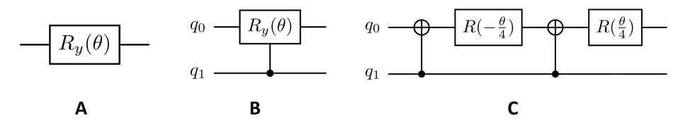
Figure 1: Schematic representations of $R_{y}$ gate, controlled-$R_{y}$ gate, and its decomposition. (A) A schematic representation of the $R_{y}$ gate with a rotation parameter $\theta$. In the representation, the input register is on the left, and the output is on the right. (B) A schematic representation of the controlled-$R_{y}$ gate with a rotation parameter $\theta$. In the representation, the control register is the qubit labeled $q_{1}$, and the target is labeled $q_{0}$. The operation is performed on the target register when the control register $q_{1}$ is $1$, and the rotation is not performed otherwise. (C) The schematic representation for the decomposition of a controlled-$R_{y}$ gate with a rotation parameter $\theta$. The sequence consists of 2 rotation gates $R(\frac{\theta}{4})$, $R(-\frac{\theta}{4})$ gates and 2 c-$NOT$ gates. The operation in the target register is equal to an $R_{y}(\theta)$ gate when the control register $q_{1}$ is 1, and no operation is performed otherwise.

2.2 The qscGRN model: a parameterized quantum circuit

In classical computation, a circuit is a model composed of a sequence of instructions (NOT, AND, OR classical gates) that are not necessarily reversible. In the classical circuit, the input bits flow through the sequence of instructions computing output bits for a certain task [35]. Similarly, a quantum circuit is a model consisting of a sequence of quantum gates that perform operations on the qubits [36]. A quantum circuit that is running an algorithm is usually initialized to $|0\rangle_{n}$, which means a string of $n$ bits of all zeros, and then put into a superposition state using $H^{\otimes n}$ transformation—which means an H gate on each qubit—allowing all possible inputs to be tested [37]. Then, the register flows through a sequence of quantum gates, and the output register is measured and decoded to interpret the result of the algorithm.

Here, we introduce the quantum single-cell gene regulatory network (qscGRN) model, that is a quantum circuit consisting of $n$ qubits, and models a biological scGRN for $n$ genes in the framework of quantum computing. A qubit in the qscGRN model represents a gene in the biological scGRN. The sequence of gates is grouped into 2 types of layers: The encoder layer $L_{enc}$ consists of $n$ $R_{y}$ gates that translate biological information (i.e., the state of gene activity or the frequency of genes actively expressed among cells) onto a superposition state. In the $L_{enc}$ layer, each qubit has a $R_{y}$ gate (FIGURE 2A). The regulation layer $L_{k}$ consists of a sequence of $n{-}1$ c-$R_{y}$ gates that have the $k$th qubit as control and a corresponding target such that the $k$th qubit is fully connected to other qubits (FIGURE 2B). In the $L_{k}$ layer, a c-$R_{y}$ gate—that has the $k$th qubit as control and the $p$th qubit as the target—models the regulation relationship in the corresponding gene-gene pair. In particular, the parameter of a c-$R_{y}$ gate quantifies the strength and determines the type of relationship between the $k$th and $p$th genes.

In FIGURE 2, we use the notation $\theta_{k,k}$ for the parameter of the $R_{y}$ gate on the $k$th qubit in the $L_{enc}$ layer and $\theta_{k,p}$ for the parameter on the c-$R_{y}$ gate in the $L_{k}$ layer that has the $k$th and $p$th qubits as control and target, respectively. Formally, the matrix representations for both layers are

$$L_{enc}=R_{y}(\theta_{n-1,n-1})\otimes\cdots\otimes R_{y}(\theta_{1,1})\otimes R_{y}(\theta_{0,0}),$$

where the $\otimes$ operator is the tensor product, and

$$L_{k}=\prod_{i=0,i\neq k}^{n-1}R_{y,n}(\theta_{k,i})=R_{y,n}(\theta_{k,n-1})\cdots R_{y,n}(\theta_{k,1})R_{y,n}(\theta_{k,0}),$$

where $R_{y,n}(\theta_{k,i})$ denotes a c-$R_{y}$ gate with the $k$th qubit as the control and $i$th qubit as the target in a $n$-qubit quantum circuit. Also, the computation of the matrix representation is not commutative, which means the order of the terms cannot be changed due to the operations needed are matrix multiplication and tensor product.

The qscGRN model is initialized to $|0\rangle_{n}$ state, and then put into a superposition state using a $L_{enc}$ layer. The gene-gene interactions are then modeled using regulation layers $L_{0}$, $L_{1}$, $\cdots$, $L_{n-1}$. Thus, the qscGRN model is a quantum circuit where each qubit is fully connected to every other qubit and has a total of $n^{2}$ quantum gate parameters. Next, we construct the matrix representation $\boldsymbol{\theta}$ of the qscGRN model using the collection of parameters $\theta_{k,p}$ on the quantum gates, where $0\leq k$, $p<n$. Therefore, the matrix representation of the qscGRN model is denoted as

$$\boldsymbol{\theta}=\begin{bmatrix}\theta_{0,0}&\theta_{0,1}&\cdots&\theta_{0,n-1}\\ \theta_{1,0}&\theta_{1,1}&\cdots&\theta_{1,n-1}\\ \vdots&\vdots&\ddots&\vdots\\ \theta_{n-1,0}&\theta_{n-1,1}&\cdots&\theta_{n-1,n-1}\\ \end{bmatrix}$$

where the diagonal elements belong to the $R_{y}$ gates in the $L_{enc}$ layer, and the non-diagonal elements to the c-$R_{y}$ gates in the regulation layers $L_{0}$, $L_{1}$, $\cdots$, $L_{n-1}$.

The output register $|\psi\rangle$ of the $n$-qubit qscGRN model, encodes the gene-gene interactions in a superposition state according to the parameter $\boldsymbol{\theta}$ and is formally defined as

$$|\psi\rangle=\left(\prod_{k=0}^{n-1}L_{k}\right)L_{enc}|0\rangle_{n}=L_{n-1}\cdots L_{1}L_{0}L_{enc}|0\rangle_{n}.$$

FIGURE 2C shows the schematic representation of a qscGRN model consisting of 4 qubits as an example for better interpretation of the equations. The quantum gate name is not shown for simplicity but only the corresponding parameter. According to the equations, the output register $|\psi_{out}\rangle$ in FIGURE 2C is defined as

$$|\psi_{out}\rangle=L_{3}L_{2}L_{1}L_{0}L_{enc}|0\rangle_{4},$$

where $L_{3}$, $L_{2}$, $L_{1}$ and $L_{0}$ have 3 parameters each, and $L_{enc}$ has 4 parameters. Then, the matrix representation $\boldsymbol{\theta}$ of the 4-qubit qscGRN model is denoted as

$$\boldsymbol{\theta}=\begin{bmatrix}\theta_{0,0}&\theta_{0,1}&\theta_{0,2}&\theta_{0,3}\\ \theta_{1,0}&\theta_{1,1}&\theta_{1,2}&\theta_{1,3}\\ \theta_{2,0}&\theta_{2,1}&\theta_{2,2}&\theta_{2,3}\\ \theta_{3,0}&\theta_{3,1}&\theta_{3,2}&\theta_{3,3}.\end{bmatrix}$$

Finally, we understand the matrix $\boldsymbol{\theta}$ as the adjacency matrix of the biological scGRN, which is a weighted directed fully connected network.

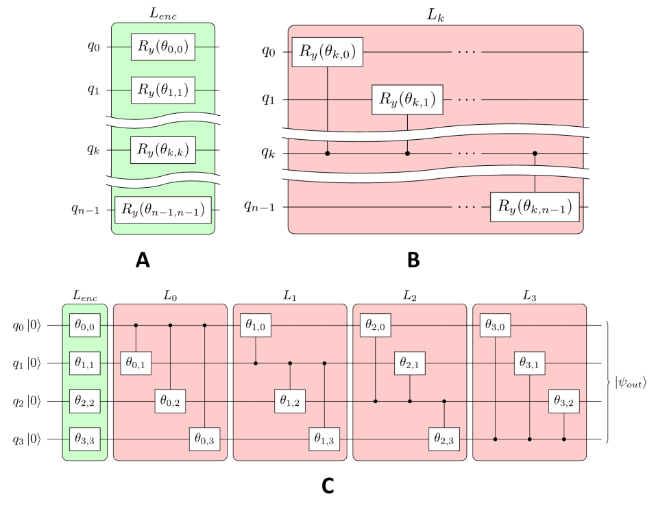
Figure 2: The quantum single-cell gene regulatory network (qscGRN) model. (A) The encoder layer $L_{enc}$ for a qscGRN model that has $n$ qubits, represented with a green background. The $k$th qubit has an $R_{y}$ gate with a parameter $\theta_{k,k}$—which is a diagonal element of the adjacency matrix in the qscGRN. (B) The regulation layer $L_{k}$ for a qscGRN model that has $n$ qubits, represented with a red background. The $k$th qubit uses a c-$R_{y}$ gate with a parameter $\theta_{k,p}$—which is a non-diagonal element of the adjacency matrix in the qscGRN—to connect to the $p$th qubit, where $0\leq p<n$ and $p\neq k$, thus the $k$th qubit is fully connected to other qubits. (C) A schematic representation of a qscGRN model that consists of 4 qubits. The $L_{enc}$ layer consists of 4 $R_{y}$ gates that put the input register into a superposition state. The $L_{k}$ layer consists of c-$R_{y}$ gates that connect the $k$th qubit to the others. Thus, a 4-qubit qscGRN model uses an $L_{enc}$ with 4 parameters and $L_{0}$, $L_{1}$, $L_{2}$ and $L_{3}$ with 3 parameters for each layer. The collection of parameters $\boldsymbol{\theta}$ is the matrix representation of the 4-qubit qscGRN model.

2.3 Quantum-classical framework for optimization of the qscGRN model

2.3.1 Gene selection and binarization

The input data of the workflow is a transformed scRNA-seq expression data matrix $\boldsymbol{X}$ that has expression values for $m$ cells. The transformation of the expression matrix can be done using, for example, Pearson residuals [38]. Then, we select $n$ genes from $\boldsymbol{X}$ and binarize the expression values. The binarization is achieved by applying an expression threshold of $0$ to the transformed expression matrix, which means that expression values greater than $0$ are set to $1$, and $0$ otherwise. The outcome of the binarization is saved to $\boldsymbol{X^{b}}$, which is a matrix of dimension $n\times m$.

2.3.2 Labeling and activation ratios (FIGURE 3A)

A label is assigned for each cell in $\boldsymbol{X^{b}}$, such that the label is a string composed of the binarized expression of the $n$ genes in a cell. In other words, a label is the activation state of genes in a cell (colored in light blue). Then, we compute the percentage of occurrences of each label in the $m$ cells to obtain the observed distribution $p^{obs}$. The percentage of label $|0\rangle_{n}$ in $p^{obs}$ is set to $0$, and the rest of the distribution is rescaled to sum to $1$. The rationale for setting the $|0\rangle_{n}$ probability to $0$ is that cells with no expression levels are not informative in the quantum framework due to dropout in the scRNA-seq experiment. Furthermore, the activation ratio $act_{k}$ of the $k$th gene is defined as the percentage of cells expressing that gene in $\boldsymbol{X^{b}}$ (colored in light yellow). The $n$ genes in $\boldsymbol{X^{b}}$ are ordered decreasingly by the activation ratio such that $\boldsymbol{X^{b}}$ has $n$ ordered rows labeled as $g_{0}$, $g_{1}$, $\cdots$, $g_{n-1}$.

2.3.3 Initialization of the parameter $\boldsymbol{\theta}$ in the qscGRN model (FIGURE 3B)

The parameters $\theta_{k,p}$ in the regulation layers $L_{0}$, $L_{1}$, $\cdots$, $L_{n-1}$ are initialized to 0, where $0\leq k,p<n$ and $k\neq p$. Besides, the parameters $\theta_{k,k}$ in the encoder layer $L_{enc}$ are initialized to $2\arcsin{\sqrt{act_{k}}}$ corresponding to the $k$th gene, where $0\leq k<n$. Therefore, the initial parameter $\boldsymbol{\theta}$ is represented as

$$\theta_{initial}=\begin{pmatrix}2\arcsin{\sqrt{act_{0}}}&0&\cdots&0\\ 0&2\arcsin{\sqrt{act_{1}}}&\cdots&0\\ \vdots&\vdots&\ddots&\vdots\\ 0&0&\cdots&2\arcsin{\sqrt{act_{n-1}}}\end{pmatrix}.$$

The rationale for the formula $2\arcsin{\sqrt{act_{k}}}$ is that, independently on each qubit, the probability of observing 1 is the activation ratio of the corresponding gene after the $L_{enc}$ layer.

2.3.4 Optimization of the parameter $\boldsymbol{\theta}$ in the qscGRN model (FIGURE 3C)

We measure the output register $|\psi_{out}\rangle$ of the qscGRN model to obtain the output distribution $p^{out}$ of observing the basis states. The probability of the state $|0\rangle_{n}$ in $p^{out}$ is set to $0$, and the rest of the distribution is rescaled to sum to $1$. Then, Laplace smoothing is used to reshape $p^{obs}$ and $p^{out}$ to a different distribution $\hat{p}^{obs}$ and $\hat{p}^{out}$, respectively, thus handling the zero-probability problem when computing the loss function. The smoothed distribution is computed as

$$\hat{p}^{i}=\frac{\#ocu^{i}+\alpha}{m+2^{n}\alpha}$$

where $i\in\{out,obs\}$ and $\alpha$ is the smoothing parameter which is typically 1. $\#ocu^{i}$ is the number of occurrences in the distribution $p^{i}$. In other words, $p^{i}{=}\tfrac{\#ocu^{i}}{m}$ is the original distribution.

The optimization of $\boldsymbol{\theta}$ is achieved by minimizing the loss function to a threshold value of $2^{n}{\times}10^{-6}$ using the gradient descent algorithm with a learning rate $lr$ of 1. Otherwise, the optimization is performed for pre-defined iterations $t$. The loss and error function are defined as

$$L(\boldsymbol{\theta})=\sum_{\mathbf{x}\in\{0,1\}^{n}}\hat{p}^{out}_{\mathbf{x}}\log{\left(\frac{\hat{p}^{out}_{\mathbf{x}}}{\hat{p}^{obs}_{\mathbf{x}}}\right)},$$

$$E(\boldsymbol{\theta})=\sum_{\mathbf{x}\in\{0,1\}^{n}}(p^{out}_{\mathbf{x}}-p^{obs}_{\mathbf{x}})^{2},$$

where $p^{i}_{\mathbf{x}}$ and $\hat{p}^{i}_{\mathbf{x}}$ are the probability of the state $\mathbf{x}$ in the distributions, $i\in\{out,obs\}$.

The parameters $\theta_{k,k}$ in the $L_{enc}$ layer are not trained during optimization according to the assumption that these parameters encode a unique binarized scRNA-seq matrix into the quantum framework. Thus, no training of the parameters $\theta_{k,k}$ implies that the $L_{enc}$ layer encodes the same biological information onto a superposition state in each iteration, making the optimized parameter $\boldsymbol{\theta}$ meaningful from a biological perspective.

2.3.5 Recovery of Gene Regulatory Network (FIGURE 3D)

We use the values of parameter $\boldsymbol{\theta}$ of qscGRN model to construct the adjacency matrix of the biological scGRN, as described in the matrix representation for qscGRN model step. In the adjacency matrix, parameters with an absolute value less than $0.087$ are set to $0$ because no significant rotation is performed by the corresponding c-$R_{y}$ gate. The heatmap representation of the adjacency matrix is shown on the left side of FIGURE 3D, where rows and columns represent control and targetgenes, respectively, and strong regulation relationships are highlighted. Finally, we construct the signed, directed, weighted network representation (right side of FIGURE 3D) of the biological scGRN using the adjacency matrix.

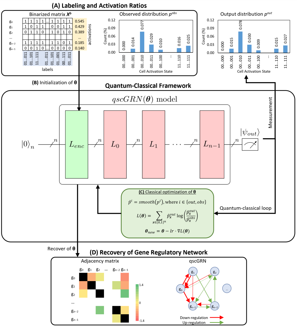
Figure 3: The quantum-classical framework using the qscGRN model to infer the corresponding biological scGRN. The input matrix $\boldsymbol{X^{b}}$ is the binarized scRNA-seq data with n genes selected. (A) Labels are assigned to each cell in $\boldsymbol{X^{b}}$ such that a label is the binarized expression string for the $n$ genes in a cell. The observed distribution $p^{obs}$ is computed as the percentage of occurrences of each label. The percentage in the $|0\rangle_{n}$ label is set to $0$, and the rest of $p^{obs}$ is rescaled. The activation ratio of a gene is the percentage of cells expressing that gene on $\boldsymbol{X^{b}}$. (B) The parameters in the $L_{enc}$ layer are initialized such that, independently, each qubit has a probability of observing $1$ equal to the corresponding activation ratio, and the parameters in $L_{0}$, $L_{1}$, $\cdots$, $L_{n}-1$ are initialized to zero. In the matrix representation of $\boldsymbol{\theta}$, the diagonal values belong to $L_{enc}$ layer, and the non-diagonal values to the regulation layers. (C) The classical optimizer fits the smoothed distributions $\hat{p}^{out}$ into $\hat{p}^{obs}$ using a gradient descent based algorithm with the KL-divergence as the loss function and the mean square as the error metric. (D) The matrix representation of the qscGRN model is used as the adjacency matrix of the biological scGRN. In the adjacency matrix, parameters smaller than $0.087$ are dropped (left side), assuming the interaction is not strong enough to report. Thus, the network representation of the biological scGRN (right side) is constructed using the remaining values in the adjacency matrix.

2.4 Data sets

LCL data set: The scRNA-seq data was generated from lymphoblastoid cell lines (LCLs), which are widely used cell model systems derived from human primary B cells. Information about the experimental handling and acquisition of data is provided in reference to our original study [28]. The data set has been deposited in the Gene Expression Omnibus (GEO) database with the accession number GSE126321. For this study, we merged this data set with another LCL scRNA-seq data set [29], for which the gene-barcode matrix files were downloaded from the GEO database using the accession number GSE158275. The raw data matrix was pre-processed using scGEAToolbox [39]. The processed matrix of $9,905$ genes and $28,208$ lymphoblastoid cells was then transformed using the Pearson residuals normalization [38]. Then, expression values of six genes (IRF4, REL, PAX5, RELA, PRDM1, AICDA) of the NF-$\kappa$B signaling pathway were extracted. The $6$-gene expression matrix ($6$-by-$28,208$) was used as the input of the qscGRN analysis of this study. The known regulatory relationships between genes were obtained from the previously established B-cell differentiation circuit model [30, 31].

3 Results

3.1 Real data LCL

We used our quantum-classical framework to build the qscGRN model—a fully connected quantum circuit—and compute the observed distribution $p^{obs}$ using the data set described in subsection 2.3.2. The input scRNA-seq expression matrix contained more than $28,000$ cells belonging to the same cell type, the lymphoblastoid cell. The $p^{obs}$ distribution maps the population of the state in the scRNA-seq data into a vector space ($p^{obs}$ is represented in blue—FIGURE 4A). The qscGRN model schema for the data set is a $6$-qubit system and consists of an encoder layer and six regulation layers (FIGURE 4B). We measured the output register of the qscGRN model to recover the output distribution $p^{out}$ from the quantum framework. To improve visualization, FIGURE 4A only shows the states with a probability greater than $0.01$ due to the large size of the vector space.

Then, we optimized the parameter $\boldsymbol{\theta}$ in the qscGRN model for $50,000$ iterations by minimizing the loss function $L(\boldsymbol{\theta})$ and using the smoothed distributions for $p^{out}$ and $p^{obs}$. Therefore, the distribution $\hat{p}^{out}$ is fitted into $\hat{p}^{obs}$ during the optimization, as shown in FIGURE 4A that visually proves the similarity of both distributions after optimization. The $p^{out}$ after optimization is represented in orange—FIGURE 4A. The similarity is quantified using the loss function and error metrics that reached values of $8.03\times 10^{-4}$ and $3.04\times 10{-5}$, respectively.

The value of the parameter $\boldsymbol{\theta}$ after optimization retrieves an adjacency matrix (FIGURE 4C) that is used to construct the biological scGRN. Then, we constructed a weighted, directed network from the quantum framework using the non-diagonal elements of $\boldsymbol{\theta}$, as shown in FIGURE 4D. We compared the sign of the element of each pair of genes with the corresponding regulatory effect in the previously published network, i.e., the baseline GRN [30, 31] . The comparison results were measured using 3 metrics: accuracy, f1 score, and precision, to quantify the prediction performance of the classical-quantum framework. The qscGRN model recovers gene-gene relationships with an accuracy, f1 score, and precision of $0.63$, $0.72$, and $0.78$, respectively.

FIGURE 4E shows the evolution of parameters for $8$ gene-gene pairs (a control-target pair) in the qscGRN model during the optimization. These pairs are relationships recovered from the quantum framework and are present in the NF-$\kappa$B network. Gene pairs correctly recovered are represented using a solid line, and pairs incorrectly recovered in long-dash-dot lines. The $8$ gene-gene pairs almost reach their optimized value by $10,000$ iterations. Specifically, pairs such as IRF4-AICDA, PAX5-AICDA, and PRDM1-PAX5 that have reached their optimized value earlier than others are strongly supported by the quantum framework. IRF4 is known to induce AICDA expression through an indirect mechanism in the NF-$\kappa$B signaling cascade [40]. PAX5 is suggested to be a player in the B-lineage-specific control of AICDA transcription in a previous study [41]. PRDM1 is a master regulator that represses PAX5 expression in B cells [42].

FIGURE 4F shows $3$ gene-gene pairs with regulatory relationships are present in the published baseline GRN but are removed by our qscGRN estimation. The exclusion of these gene pairs suggests that the regulatory relationships between them might be through indirect links. The baseline model failed to distinguish between indirect and direct links. For example, one of the removed gene pairs is IRF4-PRDM1 which has a parameter larger than $0.1$ during the first $1,000$ iterations. The parameter value decreases gradually to close to zero after $5,000$ iterations. The dropping suggests that IRF4-PRDM1’s regulatory relationship might be through a third-party modulator. Indeed, IRF4 is known to inhibit BCL6 expression, and because BCL6 can repress PRDM1 [43, 44], it has been formally speculated that the effects of IRF4 on PRDM1 expression might have been mediated through inhibition of BCL6 expression [45].

Ten novel regulatory relationships between genes, which are not in the published baseline GRN, were predicted by the qscGRN model when the computation nearly reached their optimized value by $10,000$ iterations (FIGURE 4G). We found that, for at least two of these newly discovered regulatory relationships, there is experimental evidence supporting the involved gene pairs. The first gene pair is IRF4-PAX5, for which our model predicted that PAX5 is positively regulated by IRF4. Indeed, in a previous study of the phosphoinositide-3 kinase signaling in B cells [46], an experiment searching for transcription factors that are activated by FOXO1 revealed that IRF4 is a potential candidate for PAX5 regulation. The second gene pair is PRDM1-AICDA. PRDM1 has been found to be able to silence the expression of AICDA, probably in a dose-dependent manner [47]. These results suggest that our qscGRN method recovered regulatory relationships that were missed in the published baseline model.

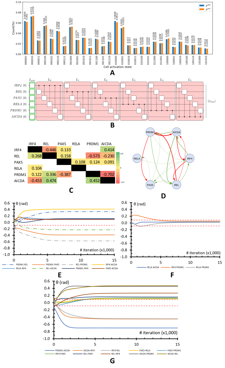
Figure 4: Application of the qscGRN modeling with real scRNA-seq data. (A) The observed and output distributions ($p^{obs}$ and $p^{out}$) colored in blue and orange, respectively. $p^{obs}$ is computed using the transformed scRNA-seq data. $p^{out}$ is obtained by measuring the output register in the qscGRN model when the optimization is completed. (B) The schematic for a $6$-genes qscGRN model consists of a $L_{enc}$ layer and six regulation layers that map relationships between genes in the quantum framework. (C) The adjacency matrix of the biological scGRN, in which parameters with an absolute value less than $0.087$ are removed. The heatmap reveals the strength and direction of the interaction for a gene-gene interaction. The diagonal elements are colored in black due to these parameters are not trained during optimization. (D) A directed-weighted representation of the biological scGRN recovered from the quantum circuit. Up-regulation and down-regulation relationships are colored in green and red, respectively. The thickness of each edge is proportional to the absolute value of the corresponding parameter in the adjacency matrix. (E) Evolution of parameters for gene-gene interaction that were recovered from the quantum framework and are present in the NF-$\kappa$B network during the first $15,000$ iterations. (F) Evolution of parameters for gene-gene interactions that were not recovered but are present in the NF-$\kappa$B network during the first $15,000$ iterations. (G) Evolution of parameters for gene-gene interaction that are predicted by the quantum framework during the first $15,000$ iterations.

4 Discussion

Finding ways to apply quantum computing in biological research is an active research area [48, 49, 50, 51]. Many questions in biology can benefit from quantum computing by exploring many possible parallel computational paths, but identifying such questions remains challenging. Especially understanding how to exploit quantum computers for progress in solving important biological questions is crucial. The latest development of scRNA-seq has made it possible to gather the transcriptome information from tens of thousands of individual cells in a high-throughput manner. These complex data sets with unprecedented detail are driving the development of new computational and statistical tools that are revolutionizing our understanding of cellular processes. However, quantum computation has not yet received enough attention in the face of this single-cell big data revolution. As a consequence, we present our qscGRN method for modeling interactions between genes to derive the quantum computing framework for constructing GRNs. Below we discuss several aspects of application issues.

4.1 Mapping of scRNA-seq data in the quantum framework

Typically, a correlation-based method obtains enough information from a scRNA-seq data set to infer a GRN with a large number of genes. The gene-gene interaction is calculated as a single value (summary statistic) using the expression values of the available cells. On the other hand, our quantum approach for GRN inference models a small number of genes due to the vector space size, which is equal to the number of basis states, increases exponentially with the number of genes. In other words, the number of cells in binarized scRNA-seq data might be mapped to a moderate number of basis states such that each basis state is mapped from the biological data. For example, a $15$-qubit qscGRN model requires $2^{15}=32,768$ basis states; however, a scRNA-seq data set with roughly $32,768$ cells would retrieve an observed distribution without meaningful biological information mapped to the basis states. The latest scRNA-seq technology has the capacity to allow the transcriptome of millions of cells to be measured. To obtain enough cells, we may also integrate multiple scRNA-seq data sets from the same cell types or similar biological sources and perform statistical correction to remove the batch effect. We can select informative genes such as highly variable genes [52] in advance, then proceed with our quantum-classical pipeline. Thus, reducing the burden of a large number of genes in the model while maintaining the biological relevance.

4.2 Initialization values for the parameter $\boldsymbol{\theta}$ in the qscGRN model

The initialization of the parameter $\boldsymbol{\theta}$ determines the starting point in the landscape of the loss function, thus indirectly setting the difficulty for the optimization due to barren plateaus—which is an issue when optimizing a parameterized quantum circuit. In subsection 2.3.3 Initialization of the parameter $\boldsymbol{\theta}$ in the qscGRN, an all-zeros approach is taken for the parameters in the c-$R_{y}$ gates. Additionally, $2$ more initialization approaches for the c-$R_{y}$ gates were tried using a random initialization with uniform and normal distributions. The $3$ methods initialize the parameter $\boldsymbol{\theta}$ at $3$ different positions in the landscape; however, only the all-zeros approach defines the same point when running the workflow again. Thus, the all-zeros approach would recover a biological scGRN consistently from the quantum framework since the gradients are computed at the same starting point. Finally, the all-zeros approach recovered $8$ gene-gene interactions with biological support, which is larger than the other approaches.

4.3 Advantages of the qscGRN over correlation- and regression-based GRNs

Correlation and regression-based methods are the most widely used methods for GRN inference due to their computational efficiency. These methods typically compute a correlation or regression coefficient for a gene pair using the total number of cells in the data. The issue with correlation and regression methods is that they rely on summary statistics. The relationship between the two genes is measured using a single value of the summary statistics: correlation or regression coefficient. Once computed, the coefficient becomes independent of the total number of cells. Moreover, increasing the number of cells would not substantially change the correlation and regression coefficients. Thus, information in the scRNA-seq data is not fully used. The other issue is that the coefficient is computed only between the two focal genes, regardless of the expression values of other genes in the same biological system. The effect of not considering other genes in the computation can result in a biased coefficient, which does not represent the true behavior of the interaction. There are methods such as partial correlation [8], principal component regression [9], and LASSO [53] that may correct this. But the correcting effect is limited given the all-to-all interactions cannot be modeled.

In contrast, our qscGRN method is based on the quantum framework, which uses the Hilbert space and maps the binarized expression of each cell for $n$ genes at once. The mapping of $n$ genes to the Hilbert space allows manipulating the superposition of basis states in an $n$ qubit system and fitting the output distribution to the observed distribution in the binarized scRNA-seq data. Thus, biological information passes through the quantum circuit and is encoded in a superposition state. In other words, a gene-gene relationship is computed using information from an $n$ gene biological system all at once in the quantum framework, which is an improvement compared to correlation-based methods.

5 Acknowledgments

This work was supported by the DoD grant GW200026 for JJC.

6 Data availability

The scRNA-seq data analyzed during the current study is available in the NCBI GEO database with the accession numbers GSE126321 and GSE158275. The processed data and the source code implementation of the qscGRN package are provided in the GitHub repository at https://github.com/cailab-tamu/QuantumGRN/. The repository also includes tutorials written in Python language.

7 Author Contributor

Conceptualization, JJC; methodology, CR and JJC; implementation of the software, CR; formal analysis, CR and JJC; writing and editing, CR and JJC; supervision, JJC. All authors reviewed and contributed to the manuscript.

8 Competing Interest

The authors declare no competing financial or non-financial interest.

References

- [1] Vân Anh Huynh-Thu and Guido Sanguinetti. Gene Regulatory Network Inference: An Introductory Survey, pages 1–23. Springer New York, New York, NY, 2019.
- [2] Michael Hecker, Sandro Lambeck, Susanne Toepfer, Eugene van Someren, and Reinhard Guthke. Gene regulatory network inference: Data integration in dynamic models—a review. Biosystems, 96(1):86–103, 2009.
- [3] Shuonan Chen and Jessica C Mar. Evaluating methods of inferring gene regulatory networks highlights their lack of performance for single cell gene expression data. BMC bioinformatics, 19(1):1–21, 2018.
- [4] Aditya Pratapa, Amogh P Jalihal, Jeffrey N Law, Aditya Bharadwaj, and TM Murali. Benchmarking algorithms for gene regulatory network inference from single-cell transcriptomic data. Nature methods, 17(2):147–154, 2020.
- [5] Léo PM Diaz and Michael PH Stumpf. Gaining confidence in inferred networks. Scientific Reports, 12(1):1–9, 2022.
- [6] Grace XY Zheng, Jessica M Terry, Phillip Belgrader, Paul Ryvkin, Zachary W Bent, Ryan Wilson, Solongo B Ziraldo, Tobias D Wheeler, Geoff P McDermott, Junjie Zhu, et al. Massively parallel digital transcriptional profiling of single cells. Nature communications, 8(1):1–12, 2017.
- [7] Thalia E Chan, Michael PH Stumpf, and Ann C Babtie. Gene regulatory network inference from single-cell data using multivariate information measures. Cell systems, 5(3):251–267, 2017.
- [8] Seongho Kim. ppcor: an r package for a fast calculation to semi-partial correlation coefficients. Communications for statistical applications and methods, 22(6):665, 2015.
- [9] Daniel Osorio, Yan Zhong, Guanxun Li, Jianhua Z Huang, and James J Cai. sctenifoldnet: a machine learning workflow for constructing and comparing transcriptome-wide gene regulatory networks from single-cell data. Patterns, 1(9):100139, 2020.
- [10] Vân Anh Huynh-Thu, Alexandre Irrthum, Louis Wehenkel, and Pierre Geurts. Inferring regulatory networks from expression data using tree-based methods. PloS one, 5(9):e12776, 2010.
- [11] Stephen Kotiang and Ali Eslami. A probabilistic graphical model for system-wide analysis of gene regulatory networks. Bioinformatics, 36(10):3192–3199, 2020.
- [12] Harri Lähdesmäki, Sampsa Hautaniemi, Ilya Shmulevich, and Olli Yli-Harja. Relationships between probabilistic boolean networks and dynamic bayesian networks as models of gene regulatory networks. Signal processing, 86(4):814–834, 2006.
- [13] Nir Friedman, Michal Linial, Iftach Nachman, and Dana Pe’er. Using bayesian networks to analyze expression data. Journal of computational biology, 7(3-4):601–620, 2000.
- [14] Ilya Shmulevich, Edward R Dougherty, Seungchan Kim, and Wei Zhang. Probabilistic boolean networks: a rule-based uncertainty model for gene regulatory networks. Bioinformatics, 18(2):261–274, 2002.
- [15] Laszlo Gyongyosi and Sandor Imre. A survey on quantum computing technology. Computer Science Review, 31:51–71, 2019.
- [16] Daniel J. Egger, Claudio Gambella, Jakub Marecek, Scott McFaddin, Martin Mevissen, Rudy Raymond, Andrea Simonetto, Stefan Woerner, and Elena Yndurain. Quantum computing for finance: State-of-the-art and future prospects. IEEE Transactions on Quantum Engineering, 1:1–24, 2020.
- [17] Tiago M. Fernández-Caramès and Paula Fraga-Lamas. Towards post-quantum blockchain: A review on blockchain cryptography resistant to quantum computing attacks. IEEE Access, 8:21091–21116, 2020.
- [18] Somayeh Bakhtiari Ramezani, Alexander Sommers, Harish Kumar Manchukonda, Shahram Rahimi, and Amin Amirlatifi. Machine learning algorithms in quantum computing: A survey. In 2020 International Joint Conference on Neural Networks (IJCNN), pages 1–8, 2020.
- [19] David Ryan Koes. The pharmit backend: a computer systems approach to enabling interactive online drug discovery. IBM journal of research and development, 62(6):3–1, 2018.
- [20] Bela Bauer, Sergey Bravyi, Mario Motta, and Garnet Kin-Lic Chan. Quantum algorithms for quantum chemistry and quantum materials science. Chemical Reviews, 120(22):12685–12717, 2020.
- [21] Kishor Bharti, Alba Cervera-Lierta, Thi Ha Kyaw, Tobias Haug, Sumner Alperin-Lea, Abhinav Anand, Matthias Degroote, Hermanni Heimonen, Jakob S. Kottmann, Tim Menke, Wai-Keong Mok, Sukin Sim, Leong-Chuan Kwek, and Alán Aspuru-Guzik. Noisy intermediate-scale quantum algorithms. Rev. Mod. Phys., 94:015004, Feb 2022.
- [22] Hsin-Yuan Huang, Michael Broughton, Jordan Cotler, Sitan Chen, Jerry Li, Masoud Mohseni, Hartmut Neven, Ryan Babbush, Richard Kueng, John Preskill, et al. Quantum advantage in learning from experiments. Science, 376(6598):1182–1186, 2022.
- [23] Peter W. Shor. Polynomial-time algorithms for prime factorization and discrete logarithms on a quantum computer. SIAM Review, 41(2):303–332, 1999.
- [24] Vaishali Bhatia and K.R. Ramkumar. An efficient quantum computing technique for cracking rsa using shor’s algorithm. In 2020 IEEE 5th International Conference on Computing Communication and Automation (ICCCA), pages 89–94, 2020.
- [25] Fuchun Peng, Dale Schuurmans, and Shaojun Wang. Augmenting naive bayes classifiers with statistical language models. Information Retrieval, 7(3):317–345, 2004.
- [26] Sebastian Ruder. An overview of gradient descent optimization algorithms, 2016.
- [27] S. Kullback and R. A. Leibler. On information and sufficiency. The Annals of Mathematical Statistics, 22(1):79–86, 1951.
- [28] Daniel Osorio, Xue Yu, Peng Yu, Erchin Serpedin, and James J Cai. Single-cell rna sequencing of a european and an african lymphoblastoid cell line. Scientific data, 6(1):1–8, 2019.
- [29] Elliott D SoRelle, Joanne Dai, Emmanuela N Bonglack, Emma M Heckenberg, Jeffrey Y Zhou, Stephanie N Giamberardino, Jeffrey A Bailey, Simon G Gregory, Cliburn Chan, and Micah A Luftig. Single-cell rna-seq reveals transcriptomic heterogeneity mediated by host–pathogen dynamics in lymphoblastoid cell lines. Elife, 10:e62586, 2021.
- [30] Koushik Roy, Simon Mitchell, Yi Liu, Sho Ohta, Yu-sheng Lin, Marie Oliver Metzig, Stephen L Nutt, and Alexander Hoffmann. A regulatory circuit controlling the dynamics of nfb crel transitions b cells from proliferation to plasma cell differentiation. Immunity, 50(3):616–628, 2019.
- [31] Roger Sciammas, Ying Li, Aryeh Warmflash, Yiqiang Song, Aaron R Dinner, and Harinder Singh. An incoherent regulatory network architecture that orchestrates b cell diversification in response to antigen signaling. Molecular systems biology, 7(1):495, 2011.
- [32] Rodney Van Meter and Mark Oskin. Architectural implications of quantum computing technologies. J. Emerg. Technol. Comput. Syst., 2(1):31–63, jan 2006.
- [33] P. A. M. Dirac. A new notation for quantum mechanics. Mathematical Proceedings of the Cambridge Philosophical Society, 35(3):416–418, 1939.
- [34] Eleanor Rieffel and Wolfgang Polak. An introduction to quantum computing for non-physicists. ACM Comput. Surv., 32(3):300–335, sep 2000.
- [35] Edward A Lee. The past, present and future of cyber-physical systems: A focus on models. Sensors, 15(3):4837–4869, 2015.
- [36] Farrokh Vatan and Colin Williams. Optimal quantum circuits for general two-qubit gates. Phys. Rev. A, 69:032315, Mar 2004.
- [37] Michele Mosca. Quantum algorithms, 2008.
- [38] Jan Lause, Philipp Berens, and Dmitry Kobak. Analytic pearson residuals for normalization of single-cell rna-seq umi data. Genome biology, 22(1):1–20, 2021.
- [39] James J Cai. scgeatoolbox: a matlab toolbox for single-cell rna sequencing data analysis, 2020.
- [40] Roger Sciammas, AL Shaffer, Jonathan H Schatz, Hong Zhao, Louis M Staudt, and Harinder Singh. Graded expression of interferon regulatory factor-4 coordinates isotype switching with plasma cell differentiation. Immunity, 25(2):225–236, 2006.
- [41] Anjana Yadav, Alexandru Olaru, Mark Saltis, Adam Setren, Jan Cerny, and Ferenc Livák. Identification of a ubiquitously active promoter of the murine activation-induced cytidine deaminase (aicda) gene. Molecular immunology, 43(6):529–541, 2006.
- [42] Michela Boi, Emanuele Zucca, Giorgio Inghirami, and Francesco Bertoni. Prdm1/blimp1: a tumor suppressor gene in b and t cell lymphomas. Leukemia & lymphoma, 56(5):1223–1228, 2015.
- [43] Chainarong Tunyaplin, AL Shaffer, Cristina D Angelin-Duclos, Xin Yu, Louis M Staudt, and Kathryn L Calame. Direct repression of prdm1 by bcl-6 inhibits plasmacytic differentiation. The Journal of Immunology, 173(2):1158–1165, 2004.
- [44] Miriam Shapiro-Shelef and Kathryn Calame. Regulation of plasma-cell development. Nature Reviews Immunology, 5(3):230–242, 2005.
- [45] Yuou Teng, Yusuke Takahashi, Makiko Yamada, Tetsuya Kurosu, Takatoshi Koyama, Osamu Miura, and Tohru Miki. Irf4 negatively regulates proliferation of germinal center b cell-derived burkitt’s lymphoma cell lines and induces differentiation toward plasma cells. European journal of cell biology, 86(10):581–589, 2007.
- [46] Hend Abdelrasoul, Markus Werner, Corinna S Setz, Klaus Okkenhaug, and Hassan Jumaa. Pi3k induces b-cell development and regulates b cell identity. Scientific reports, 8(1):1–15, 2018.
- [47] Stephen L Nutt, Nadine Taubenheim, Jhagvaral Hasbold, Lynn M Corcoran, and Philip D Hodgkin. The genetic network controlling plasma cell differentiation. In Seminars in immunology, volume 23, pages 341–349. Elsevier, 2011.
- [48] Carlos Outeiral, Martin Strahm, Jiye Shi, Garrett M. Morris, Simon C. Benjamin, and Charlotte M. Deane. The prospects of quantum computing in computational molecular biology. WIREs Computational Molecular Science, 11(1):e1481, 2021.
- [49] Vivien Marx. Biology begins to tangle with quantum computing. Nature Methods, 18(7):715–719, 2021.
- [50] Prashant S Emani, Jonathan Warrell, Alan Anticevic, Stefan Bekiranov, Michael Gandal, Michael J McConnell, Guillermo Sapiro, Alán Aspuru-Guzik, Justin T Baker, Matteo Bastiani, et al. Quantum computing at the frontiers of biological sciences. Nature Methods, 18(7):701–709, 2021.
- [51] Hai-Ping Cheng, Erik Deumens, James K Freericks, Chenglong Li, and Beverly A Sanders. Application of quantum computing to biochemical systems: A look to the future. Frontiers in Chemistry, 8:587143, 2020.
- [52] Daniel Osorio, Xue Yu, Yan Zhong, Guanxun Li, Erchin Serpedin, Jianhua Z Huang, and James J Cai. Single-cell expression variability implies cell function. Cells, 9(1):14, 2019.
- [53] Robert Tibshirani. Regression shrinkage and selection via the lasso. Journal of the Royal Statistical Society: Series B (Methodological), 58(1):267–288, 1996.