Learning Citywide Patterns of Life from Trajectory Monitoring
Abstract.
The recent proliferation of real-world human mobility datasets has catalyzed geospatial and transportation research in trajectory prediction, demand forecasting, travel time estimation, and anomaly detection. However, these datasets also enable, more broadly, a descriptive analysis of intricate systems of human mobility. We formally define patterns of life analysis as a natural, explainable extension of online unsupervised anomaly detection, where we not only monitor a data stream for anomalies but also explicitly extract normal patterns over time. To learn patterns of life, we adapt Grow When Required (GWR) episodic memory from research in computational biology and neurorobotics to a new domain of geospatial analysis. This biologically-inspired neural network, related to self-organizing maps (SOM), constructs a set of “memories” or prototype traffic patterns incrementally as it iterates over the GPS stream. It then compares each new observation to its prior experiences, inducing an online, unsupervised clustering and anomaly detection on the data. We mine patterns-of-interest from the Porto taxi dataset, including both major public holidays and newly-discovered transportation anomalies, such as festivals and concerts which, to our knowledge, have not been previously acknowledged or reported in prior work. We anticipate that the capability to incrementally learn normal and abnormal road transportation behavior will be useful in many domains, including smart cities, autonomous vehicles, and urban planning and management.
T
1. Introduction
What can we learn from observing the mobility of human populations? The study of human movement and its properties, causes, motivations, and constraints has a long and storied history, dating to at least the 19th century (see (Barbosa et al., 2018) for a review). In its most modern form, the field increasingly uses a proliferation of positioning systems, including GPS, cell towers, and WiFi, to mine individual- and population-level patterns-of-interest (Toch et al., 2019). Geospatial professionals such as city planners, transportation managers, and ride-sharing developers have a compelling need to understand patterns of normal behavior and detect deviations from them in real time.
However, incrementally learning patterns from data streams poses unique challenges for machine learning (ML) systems. Over time, any number of factors may alter the statistical distribution of the data stream. Some neighborhoods grow, and others decline; new businesses open, and old ones close their doors; a tourism boom may boost traffic, or an unexpected pandemic may shrink it rapidly. These concept drifts are a significant danger to ML systems. Models pre-trained on historical data are unable to adapt to the altered patterns, but conversely, ML systems that naïvely train on new data will instead forget older information which may be useful in the future. Since each gradient update optimizes only for the current mini-batch, and not previous historical data, any learned knowledge is rapidly forgotten in subsequent weight updates. This problem is commonly known as catastrophic forgetting.
A second issue for many ML methods, especially in deep learning, is the difficulty of explaining or interpreting their internal reasoning. As a result, they are often described as “black box” models. For anomaly detection, this is particularly problematic: with neither ground-truth labels nor interpretable reasoning, end users have little basis to trust the model’s decisions. Taken together, these distinct challenges combine into a much greater problem. We know that any “black box” system will encounter concept drifts, but because we cannot inspect the model’s reasoning or compare its predictions with ground truth, we cannot easily assess these drifts and their harmful effects on the model.
Instead, we propose an approach which borrows a modeling framework from computational biology and neurorobotics, two disciplines which have long researched how real-life organisms operate under dynamically changing environments and applied these insights to artificial systems. The proposed approach uses Grow When Required (GWR) networks of bio-inspired episodic memories, which are explicitly designed to acquire unsupervised knowledge over time and protect it from subsequent degradation. We ensure that all encoded knowledge is accessible throughout and after the learning process: a set of normalcy patterns, or patterns of life, enabling the model to detect and explain any deviations from typical aggregate mobility behavior. As an example, the proposed system detects multiple culturally important events in the classic Porto taxi dataset which, to our knowledge, have not been reported or modeled in previous work. We envision that these patterns-of-life models will be very useful in continually mining unsupervised GPS streams, due to their natural robustness to concept drifts, especially in domains where human-machine trust is paramount.
2. Related work
2.1. Machine learning and human mobility
The growth of large-scale public mobility datasets has encouraged a parallel development of machine-learning methods to generate predictions and mine patterns of interest from data (as reviewed by Toch et al. (2019)). In the unsupervised setting most relevant to this work, researchers often use clustering methods, especially -means (Ashbrook and Starner, 2003; Cao et al., 2010; Andrienko et al., 2012; Reades et al., 2007), and density-based (Nanni and Pedreschi, 2006; Cao et al., 2010; Lee et al., 2007; Pelekis et al., 2009; Andrienko et al., 2011) clustering. Hierarchical (Ying et al., 2014; Lin et al., 2013) and spectral clustering (Rösler and Liebig, 2013) may also be used to group related users, places, or trajectories, and generative topic models such as latent Dirichlet allocation may reveal underlying routines or lifestyles (Farrahi and Gatica-Perez, 2011; Zion and Lerner, 2017; Deb and Basu, 2015). Some recent works have incorporated variational autoencoders (Gao et al., 2019), graph convolutional networks (Jenkins et al., 2019), and spectral graph wavelets from manifold learning (Watson et al., 2020).
Recently many authors have used taxicab data-sets for targeted prediction problems, such as prediction of GPS points within the trajectory (including the final destination and/or arbitrary points) (De Brébisson et al., 2015; Zhang et al., 2018; Rossi et al., 2019; Zhang et al., 2019; Li et al., 2020; Ebel et al., 2020; Liao et al., 2021), passenger demand (Moreira-Matias et al., 2013; Saadallah et al., 2018; Le Quy et al., 2019; Rodrigues et al., 2020), and travel time (Hoch, 2015; Gupta et al., 2018; Fu and Lee, 2019; Lan et al., 2019; Das et al., 2019; Abbar et al., 2020). A smaller community of authors has also used these data-sets to develop unsupervised methods which aim to detect unusual or anomalous trajectories (Lam, 2016; Wu et al., 2017; Keane, 2017; Irvine et al., 2018; Song et al., 2018; Liu et al., 2020). Lam (2016) employs a nearest-neighbor search to determine anomalous driving behavior; Irvine et al. (2018) compute a probability distribution over learned sequences from tokenized trajectories; Wu et al. (2017) use a reinforcement model of driver preferences and behavior. Other authors train recurrent neural networks in both supervised and unsupervised settings. Song et al. (2018) label a set of trajectories as anomalous and train a model to classify them, while Liu et al. (2020) propose a deep recurrent variational autoencoder.
2.2. Approaches to lifelong learning
The problem of catastrophic forgetting in neural networks was first reported more than 30 years ago (McCloskey and Cohen, 1989; Ratcliff, 1990) and has been a highly active research domain ever since. The resulting literature of lifelong learning (a.k.a. continual learning, incremental learning) has largely crystallized into three distinct approaches (see (Parisi et al., 2019) for a thorough review). First, replay (a.k.a. rehearsal) simply stores a small set of training inputs (such as, but not always, an online random sample) and periodically retrains the model on it (Isele and Cosgun, 2018; Riemer et al., 2019; Chaudhry et al., 2019; Kim et al., 2020). Second, more complex regularization approaches such as (Li and Hoiem, 2017; Kirkpatrick et al., 2017; Zenke et al., 2017) all add additional loss functions to encourage the model to preserve some previous knowledge while training on new data. Finally, and most relevant to our work, dynamic architectures change structural properties of the network itself to accomodate the incremental accumulation of new knowledge. Neurons can be inserted or removed; their connections, rewired into entirely new synaptic organizations; entire sets of weights, “frozen” or trained depending on the input stream. The scale of changes could be as small as a single neuronal unit or can expand to mutate large sub-networks of the model, e.g., (Zhou et al., 2012; Xiao et al., 2014; Rusu et al., 2016; Draelos et al., 2017; Yoon et al., 2018).
One of the most well-studied families of dynamic neural architectures is the self-organizing map (SOM), developed by Kohonen in the early 1980s (e.g., (Kohonen, 1982)). SOMs consist a set of neurons, or units, undergoing competitive learning: each training example is matched to a unit with the most similar features (the best-matching unit, or BMU), and used to train the BMU and other nearby units within a predefined neighborhood function. A later, but similar, alternative is the neural gas, which introduced connections between related neurons (Martinetz and Schulten, 1991), i.e., the famous Hebbian learning principle that “cells that fire together, wire together.” Neither of these formulations allows for neurogenesis, or the creation of new neurons. However, they inspired a vast array of new “growing” networks, many explicitly intended for lifelong learning applications (Bauer and Villmann, 1997; Fritzke et al., 1995; Prudent and Ennaji, 2005; Marsland et al., 2002). Most importantly for this work, the grow when required (GWR) network (Marsland et al., 2002) introduced a biologically-inspired habituation mechanism for a network to adjust its size in response to inputs.
These networks have been especially well-studied for autonomous agents and neurorobotics (Jun and Duckett, 2003; Neto and Nehmzow, 2007; Parisi et al., 2018; Ezenkwu and Starkey, 2019; Contreras-Cruz et al., 2019; Pitonakova and Bullock, 2020; Duczek et al., 2021), including by the original authors of GWR (Marsland et al., 2005), because these kinds of networks coincide with a key intrinsic motivation of any autonomous system: to progressively learn to ignore sensory inputs which are already well-known, and to identify anything else (Nehmzow et al., 2013). This principle is not unique to robotics, also finding applications as diverse as retail sales (Decker, 2005), action and emotion recognition (Parisi et al., 2017; Mici et al., 2018; Barros et al., 2019), video surveillance (Acevedo-Rodríguez et al., 2011; Sun et al., 2017), medical imaging (Angelopoulou et al., 2005; de Oliveira Martins et al., 2009; Netto et al., 2012), and genomics (Todorov et al., 2020). However, few authors have applied any SOM or related method to transportation applications (rare exceptions include (Rudloff and Ray, 2010; Lopez et al., 2017; Beura et al., 2018)), and to our knowledge, we are the first to apply either GWR or a lifelong-learning SOM to this domain.
3. Problem Description
Let be the data stream of all trajectories in the dataset, in order of occurrence, where a trajectory is a variable-length series of latitude-longitude points . For computational convenience (to calculate distances in meters and kilometers simply), we transform these into UTM coordinates .
We assume that for each trajectory , there are some number of latent factors which influence , most notably the geospatial probability distribution of where originates. Examples might include city-wide factors such as tourist volume, weather, or academic schedules and geospatially-local factors such as new construction or road closures. The identity of all the factors , or even the number of factors , is itself impossible to observe and intractable to learn. However, we know that (some subset of) may vary over time. Therefore, even without observing directly, we aim to detect changes in by observing changes in the trajectory stream .
Our problem, then, is to continually monitor a GPS trajectory stream , here from the Porto taxi dataset, and learn to construct a model of ’s normal behavior without supervision. When an interval of trajectories , taken in the aggregate, deviates from ordinary behavior, must detect the anomaly and provide enough spatiotemporal explanation of its own reasoning that a human observer can interrogate the purported anomaly (often called a “white box” model). We consider an anomaly detection correct if, and only if, both of the following conditions are met: (1) the model provides sufficient explanation of its reasoning that a human user can quickly search for sociocultural information to confirm or reject the detection, and (2) the detection is in fact accurate: additional pieces of evidence, such as contemporaneous sources, confirm a plausible explanation for unusual activity in the specified location and time.
The model can detect changes in the data stream ; the human-model team can detect changes in the cultural factors . This is a notably more difficult problem than ordinary anomaly detection, which is typically only concerned with detection accuracy relative to a provided ground truth. Instead, our problem formulation mandates explanation and interaction between and a human partner: we only count an anomaly detection as correct if it has a human-readable explanation. However, we argue that in the setting of fully unsupervised learning, requiring human-in-the-loop explanation and validation is essential in order to establish trust in the final model.
4. Methods
4.1. Interpretation of a trained GWR network
One of the advantages of a GWR network, as opposed to a “black box” model such as a deep neural network, is that each component provides a convenient interpretation. The GWR can be viewed as an online clustering of the data stream. Each neuron has a weight vector which represents a prototype input (such as a GPS location or citywide traffic pattern), and the model seeks to find a limited set of prototypes which are adequate to match all observations. We will show in Sections 5.2 and 5.3 that a properly-constructed set of prototypes can be viewed as a model of the trajectory stream ’s normal behavior, with each representing a different sub-type of “behavior.” We refer to these prototypical behaviors, operationalized as GWR weight vectors, as the patterns of life extracted from the data stream. Unlike some techniques such as -means or Gaussian mixtures, the number of prototypes need not be known in advance or tuned as a hyperparameter: it will be learned during model training.
Each neuron also has a habituation, a scalar value which can be viewed as an inverse of the probability mass or support of each prototype. It is possible to recover from an approximate measure of how frequently neuron was activated, that is, the proportion of observations with which neuron is associated.
The GWR can also be viewed as a one-layer autoencoder, a type of (typically deep) neural network which accepts an input and attempts to learn a function to reconstruct it, given information constraints. These autoencoders are frequently used for unsupervised anomaly detection, where a sudden increase in reconstruction error implies an input which does not match the model’s training set. Note that the error described below is, essentially, a -based reconstruction loss (Eq. 2), and the update formula for (Eq. 7) a gradient descent step to minimize this loss. As in many unsupervised anomaly detections, an increase in the reconstruction loss (or equivalently, drop in ) implies an anomaly, but instead of a black-box result, the input can be compared element-wise with the most relevant prototype, (see Figs. 5 and 6).
4.2. Detailed training procedure
We describe the GWR algorithm formally in this section. For hyperparameter values and a graphical depiction of the algorithm, please refer to the Appendix.
4.2.1. Initialization
We begin with a set of two neurons represented by their weight vectors, . We also require a representation of whether two neurons are connected; we use a (sparse) adjacency matrix . Note that this graph is undirected and must remain symmetric. For brevity, we will omit duplicate assignments to , but any equality or assignment also implies . We will use the notation to refer to the neighbors of neuron , that is, the set .
4.2.2. Finding matching units
We begin iterating over each input in the data stream. We find the best matching unit (BMU) , the neuron with the least distance to the input . We also find the second-best matching unit similarly, by finding the BMU of all neurons except ,
| (1) |
A connection between and is made, if it does not already exist, by setting . This forms a synapse between the best two neurons for the given input, analogous to Hebbian learning principles from neurobiology (Martinetz and Schulten, 1991).
4.2.3. Network activity
We calculate the activity of the network, , as a simple transformation of the network’s reconstruction error ,
| (2) |
Note that this provides a performance metric which the network seeks to optimize. A perfect reconstruction results in , whereas .
4.2.4. Neurogenesis
More importantly, however, the activity provides us a criterion to control the creation of new neurons. Note that represents the performance of the best matching unit: by definition, all the other neurons perform worse for this particular input . Therefore, if is low, then none of the units matched the input well.
If is below an activity threshold , we add a new neuron ,
| (3) | ||||
| (4) |
In other words, the weights of the new neuron are the average of the input and the best-matching unit . In the adjacency matrix , is inserted between the two neurons with the best reconstruction and , so that it is connected to each of them, but they no longer connect to each other.
4.2.5. Neuron update
If, and only if, the activity threshold above is not reached, we instead update the weights for the BMU and any other neuron attached to it . A simple update rule would be,
where is a learning rate for neuron . In practice, it is typical to use a relatively large learning rate for the BMU, , and a smaller learning rate for its neighbors.
4.2.6. Final steps
The iteration concludes by altering ’s connections to neurons other than in the adjacency matrix . Until this point, we have only inserted zeros and ones into . However, the elements of actually represent synapse “ages,” that is, is the number of examples observed since and matched together as the two best neurons. We increment the age of all ’s synapses, other than .
| (5) |
Recall that we already reset the age of the – synapse to previously (Section 4.2.2). If a synapse exceeds a certain age threshold it may be safely pruned, and if a neuron loses all connections then it may also be removed from the GWR network. This concludes the processing of the input , and we loop back to Section 4.2.2 and repeat for each input in the data stream.
4.2.7. Habituation
The above GWR implementation is nearly complete, but one issue remains. Note that neurogenesis (Section 4.2.4) and neuron updates (Section 4.2.5) are mutually exclusive. Since the network is initially untrained, the activity will likely be low and a new neuron will be created—precluding any training of existing neurons. For the next input, the existing neurons will remain poor, creating another new neuron—and preventing training. This loop of repeated neurogenesis leads to a network much larger then it needs to be; a smaller set of well-trained neurons would have been adequate. After all, the GWR network should only grow when required.
The solution is habituation, a computational model of how synapses lose efficacy as they are repeatedly activated (Stanley, 1976; Marsland et al., 2002). We modify the definition of a neuron to include both its weight vector and a scalar firing counter, which is initialized to . Crucially, decays each time is trained, as shown below. Therefore, during training will give us a measure of whether neuron is old and well-trained, or newly-formed and in need of tuning.
Habituation provides the network with two desirable properties. First, adding a new neuron requires not only that (see Section 4.2.4), but also that the best-matching unit have for some firing threshold . If is close to 1, then has not yet been adequately trained, and the network will choose to improve its weights rather than adding a new neuron.
Second, we modify the rules for updating neurons presented in Section 4.2.5:
| (6) | ||||||
| (7) | ||||||
where and are additional hyperparameters controlling the rate of habituation. Like the learning rates , the rate is larger for the BMU than its neighbors .
Note that decreases whenever is updated (Eq. 6) and also controls the size of ’s update (Eq. 7). Therefore, the more neuron is trained, the more resistant it becomes to training. This helps to prevent catastrophic forgetting when the data stream changes, by explicitly preventing the degradation of knowledge stored within well-trained neurons.
4.2.8. Summary
Suppose example is best-matched with BMU . The network’s performance is the activity . There are three cases to consider:
-
(1)
The activity is close to 1: The GWR network performs well. The weight will be updated, but the magnitude of the term is small. As a result, does not change much (Eq. 7).
-
(2)
The activity is below the threshold , but the firing counter is not yet below its threshold : The best-matching unit performs poorly, but its weights are based on relatively little training data. Therefore, we train the weights . The magnitude of (Eq. 7) is large, and will change more significantly.
-
(3)
The activity is below the threshold , and the firing counter is below threshold : The best-matching unit performs poorly, but its weights have been trained previously on large amounts of data. Rather than degrade that pre-existing knowledge with a weight update (causing catastrophic forgetting), we preserve it and insert a new neuron instead.
5. Results
Taxicabs are a particularly rich source of publicly-accessible research data, including from Porto (Moreira-Matias et al., 2013), San Francisco (Piorkowski et al., 2009), New York City (NYC Taxi & Limousine Commission, nd), Rome (Bracciale et al., 2014), and Beijing (Yuan et al., 2010). Of these, the Porto dataset has been especially thoroughly researched since its 2015 release for a ECML/PKDD machine learning competition. Here, we present the results of our model using the Porto dataset.
5.1. Partitioning Porto with GWR
Our approach uses a hierarchical GWR with two levels. In the first level, we spatially partition the Porto area into sub-regions learned alongside the second-level anomaly detector. Let be the stream of all trajectories in the dataset, in order of occurrence. Let be the originating point of the trajectory at time , that is, the point at which the driver picks up the passenger. We input each into a GWR where each neuron learns a two-dimensional weight vector and iterate over all trajectories in the dataset. The hyperparameters for this GWR can be found in the Appendix.
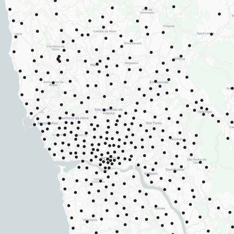
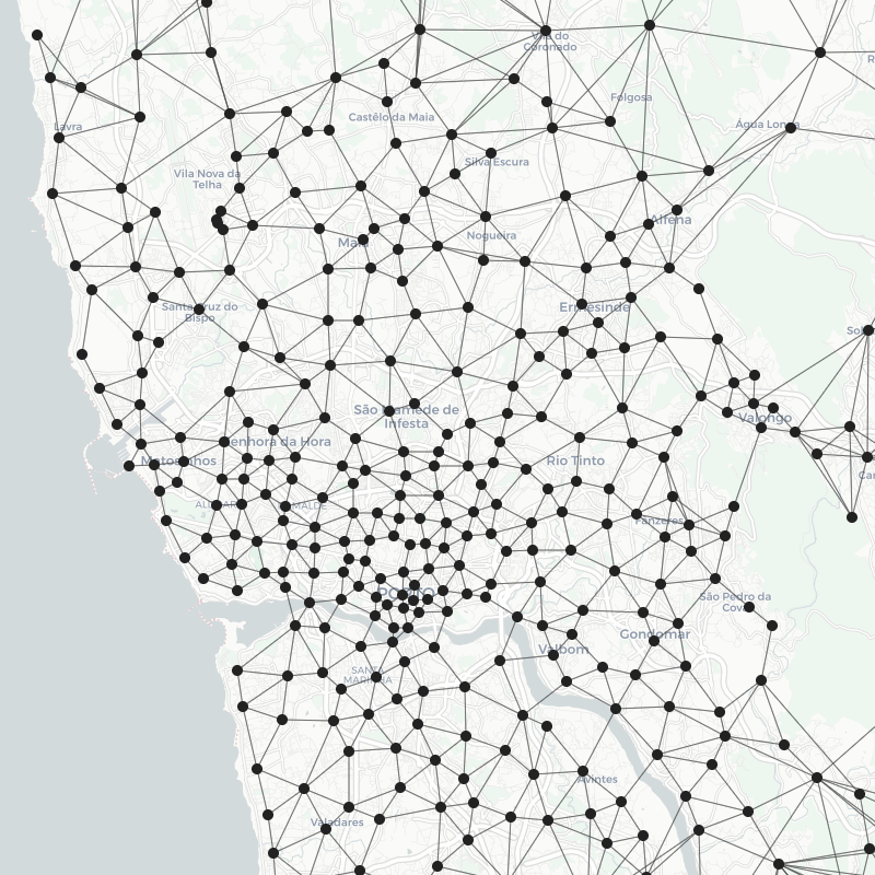
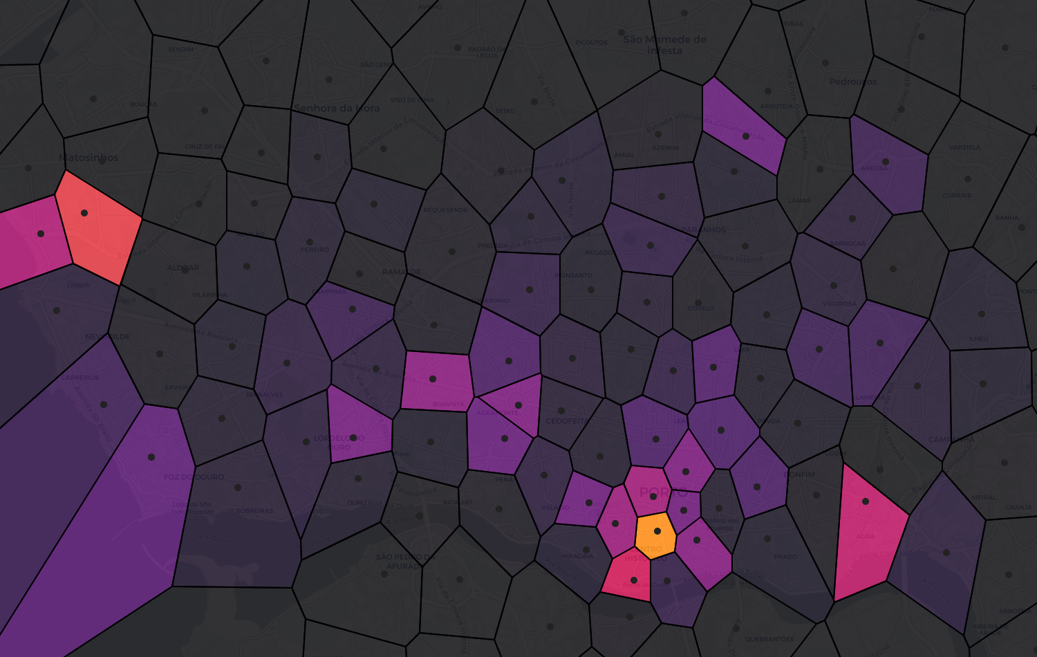
We display the results of this origin-point GWR in Fig. 2(a). On the left, we depict only the prototype origin points . Note that regions with high traffic density (e.g., downtown) have a high density of neurons compared to suburban and rural areas. This illustrates the effects of habituation (Eq. 6) on neurogenesis; the GWR is only allowed to create new neurons when , which occurs in regions with high data density where neurons are frequently activated. Note also that there seems to be a minimum distance between neurons even in high-density regions. This is a consequence of the activity threshold: new neurons can only be created if . Because of the relationship between and (Eq. 2), there is a one-to-one mapping between an activity threshold , such that neurogenesis only occurs for low , and a distance threshold such that neurogenesis only occurs when the best neuron’s error . This allows us to control the distance between neurons; for example, to only create neurons when an input point is at least km from all the network’s neurons, we set . In Fig. 2(b), we further display the synapses . Recall that since synapses are added between two neurons and which are the closest to some point ; thus, tends to connect neurons which are spatially proximate.
Although our data come from GPS rather than visual data, the structure of GWR results in a close analogy to the early processing stages of biological vision (for a review, see (Spillmann, 2014)). In biological vision, any given optic nerve fiber will only respond to inputs within a restricted sub-region of the overall visual field, known as that fiber’s receptive field (Hartline, 1938). Evidence suggests that each receptive field maps to an equal amount of space in the brain’s cortex, i.e., an equal amount of processing and subjective “perception” (Ransom-Hogg and Spillmann, 1980; Hubel and Wiesel, 1974). However, each field represents a differently-sized input region. In the fovea (the visual field’s center), many small receptive fields are packed closely together; in the periphery, larger fields are spread apart. The relationship between the size of a receptive field and its distance from the fovea is approximately linear (Hubel and Wiesel, 1974). Because receptive fields are more densely packed in the fovea, and each field receives equal cortical processing, this structure gives rise to a subjective experience of detailed high-resolution visual experience in the center of the visual field, combined with blurry low-resolution peripheral vision.
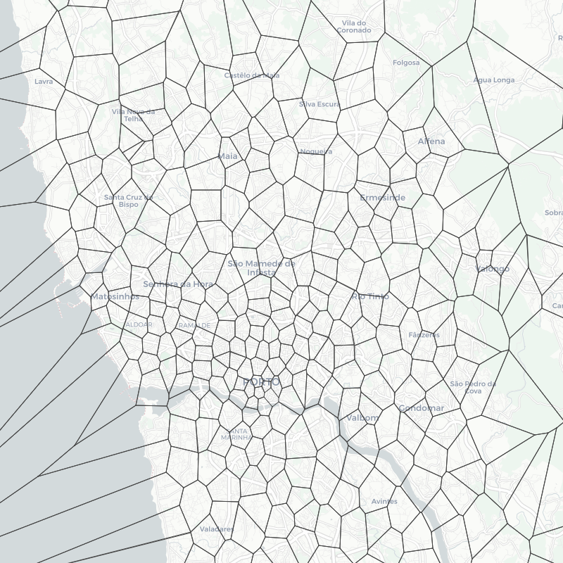
In our system, the computation of the receptive fields is a Voronoi decomposition (Fig. 2(c)). Just as we can determine a best-matching unit given some input point , we can choose a region of points for which a specific neuron would be the BMU,
| (8) |
which forms a partition of the input space. In areas of the input space densely packed with neurons (e.g., downtown), receptive fields are quite small; conversely, in areas with a low density of neurons, receptive fields are larger—closely mimicking biological vision. The connection between GWR (and related methods) and Voronoi decompositions has long been key to their development (Fritzke et al., 1995; Marsland et al., 2002). In practice, these Voronoi regions provide a better tokenization of the GPS input space than many popular alternatives: a set of regions which can be constructed incrementally, with guarantees that they (i) partition the full input space (any can be assigned to a region), (ii) always are convex polyhedra, and (iii) adapt to the statistical density of the underlying data stream. As in biological vision, we ensure that each receptive field receives equal processing in higher-level analysis regardless of its size, by treating each as a separate feature with equal scale (as described below).
5.2. Modeling normal and anomalous dates
As alluded to above, our anomaly-detection framework incorporates two levels of GWR. In the second, we consider all trajectories from a given day. Each one has a BMU , a single neuron in the first-level GWR described above, implying an ordered list of neuron indices .
At the end of each day, we calculate a new input vector by finding the proportion of trajectories which occurred in each region. This forms the input of a second GWR. The Porto dataset, which is one year long, thus defines a sequence of 365 input vectors , each of which represents a density of taxis originating in each region that day. We represent the properties of this second GWR as , , , , etc. to distinguish them from the first GWR. All hyperparameters can be found in the Appendix.
An unusual trait of this approach is that the size of the input can change, since it has one entry for each neuron in the first GWR, which is itself growing. GWR implementations with input vectors of varying size are rare (although (Pitonakova and Bullock, 2020) is an exception). However, we note that if a new neuron (i.e., Voronoi region) is created in the first GWR at time , then by assumption the previous traffic in that region should be 0 (it did not exist previously). Therefore, a simple implementation is to concatenate a 0 into previous memories for the new region, .
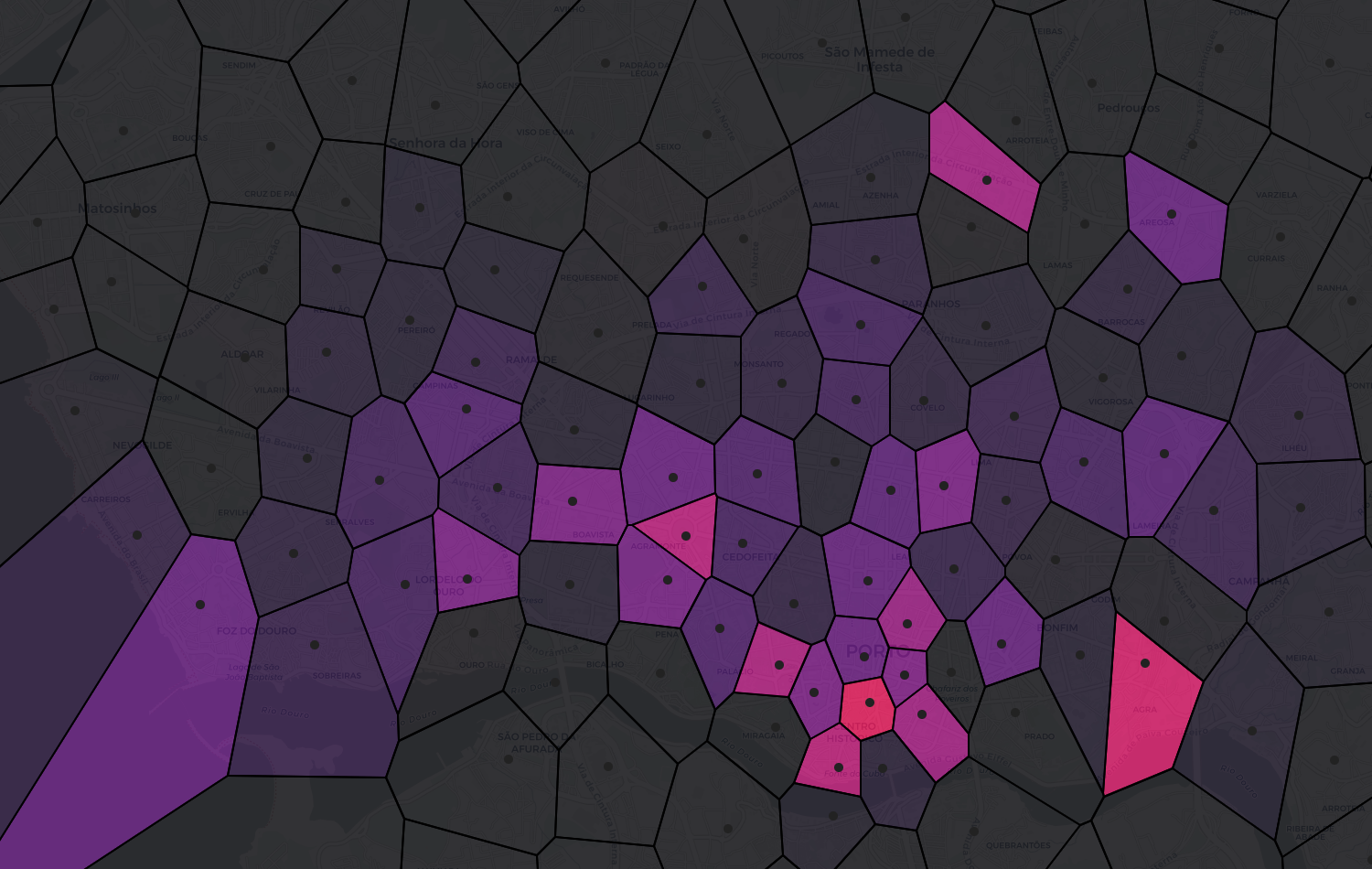
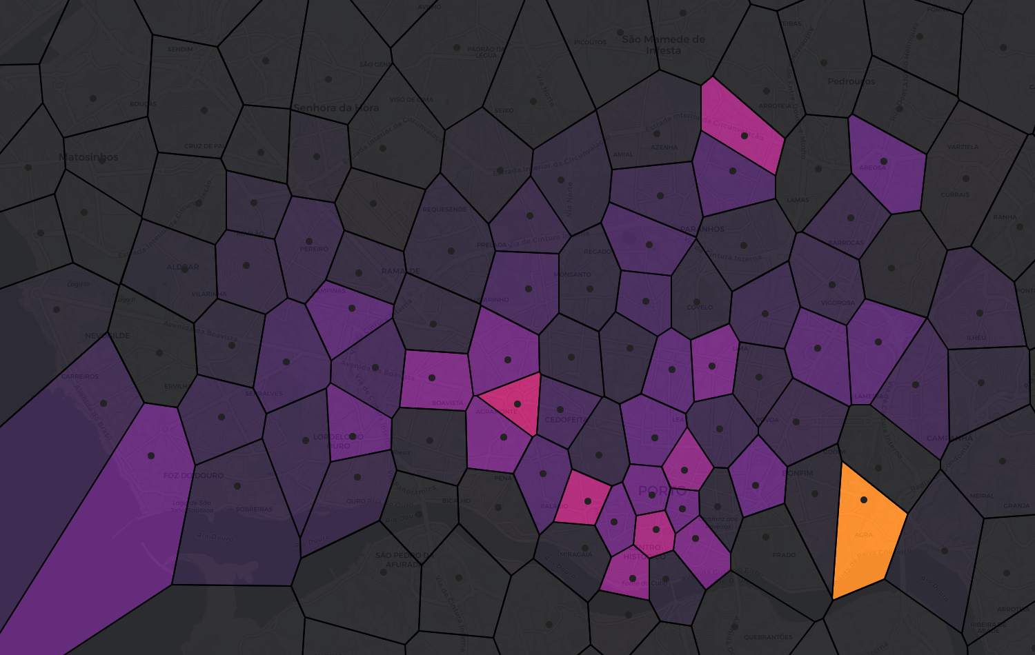
In Fig. 3, we visualize a selection of neurons from this higher-level GWR after training on the Porto dataset. Each neuron represents a prototype of an aggregated daily traffic distribution, and each actual observed day can be matched to a single prototype pattern, the best-matching unit . A large distance on day between an input and its BMU implies a low activity score . Thus, we can calculate this metric once per day and monitor it for any sudden drop in value, hinting at the existence of an unusual event or anomaly.
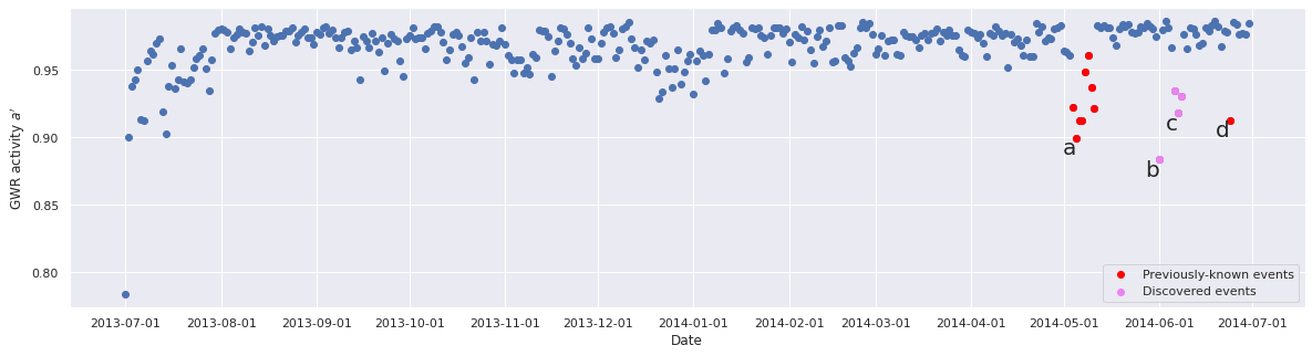
Based on our cultural research, we anticipated that we would find at least two major anomalous dates: (i) Queima das Fitas (“Burning of the Ribbons”), an eight-day festival from May 4–11, 2014, and (ii) Festa de São João do Porto (St. John’s festival) on June 23, 2014. As can be seen in Fig. 4, we can observe significant and sudden drops in the activity value which coincide with these events. The activity score also is slightly depressed during the holiday season, from the weekend before Christmas through New Year’s Day.
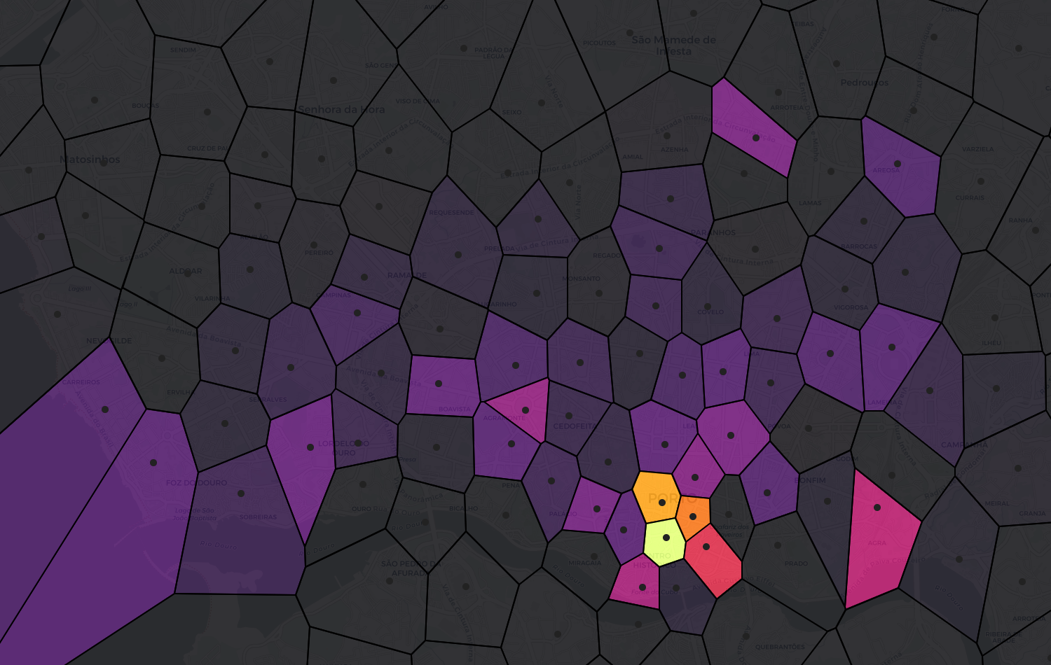
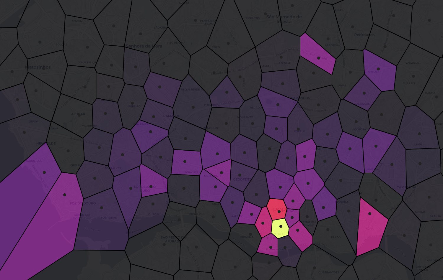
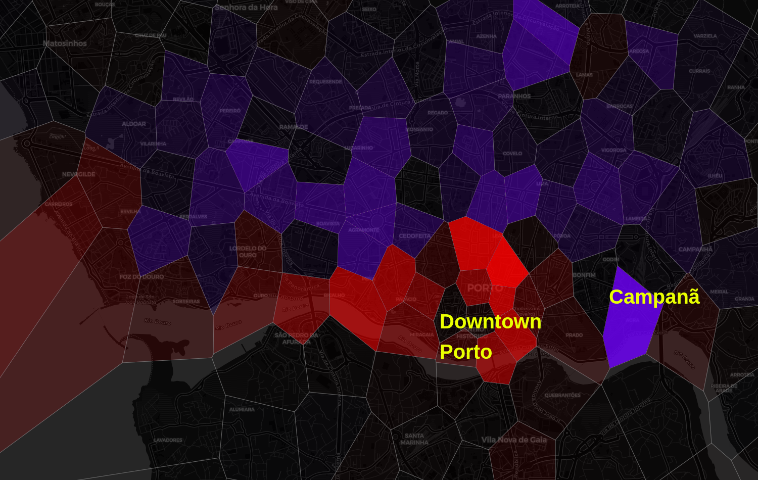
The BMU weights represent a predicted relative taxi volume in each Porto region for the given day, which can be compared directly to the actual observed pattern to see which regions had more (or less) traffic than than expected. In Fig. 5, we illustrate region-wise deviations from typical behavior in detail.
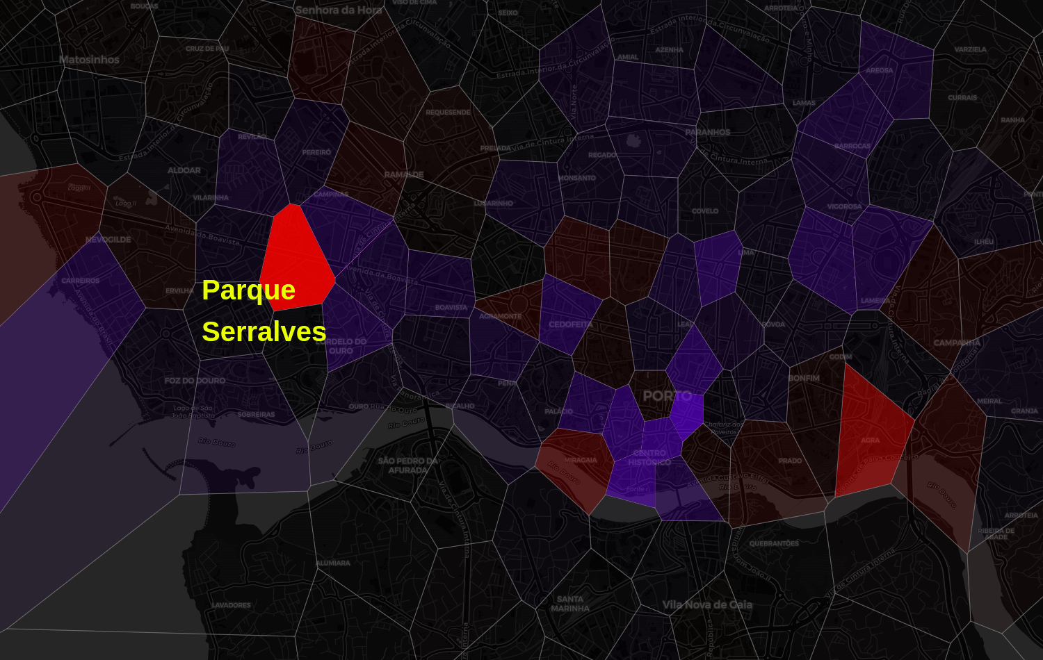
5.3. Uncovering new events within Porto
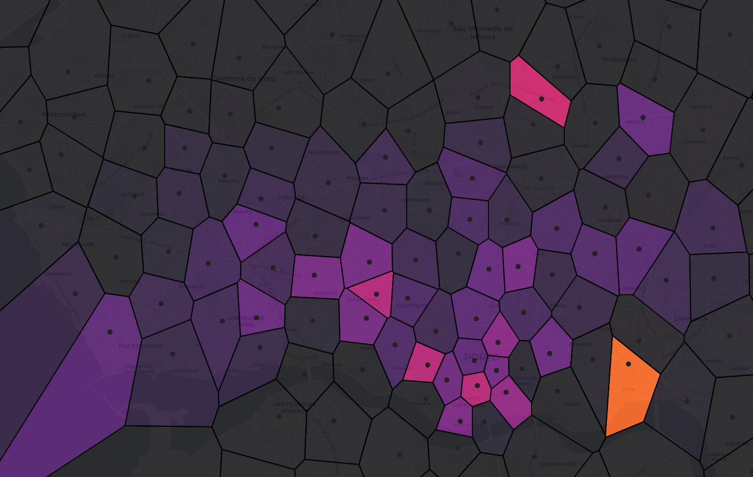
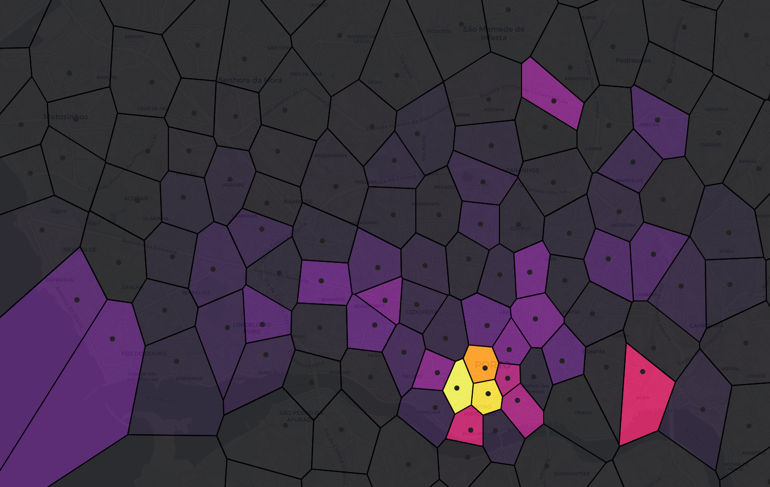
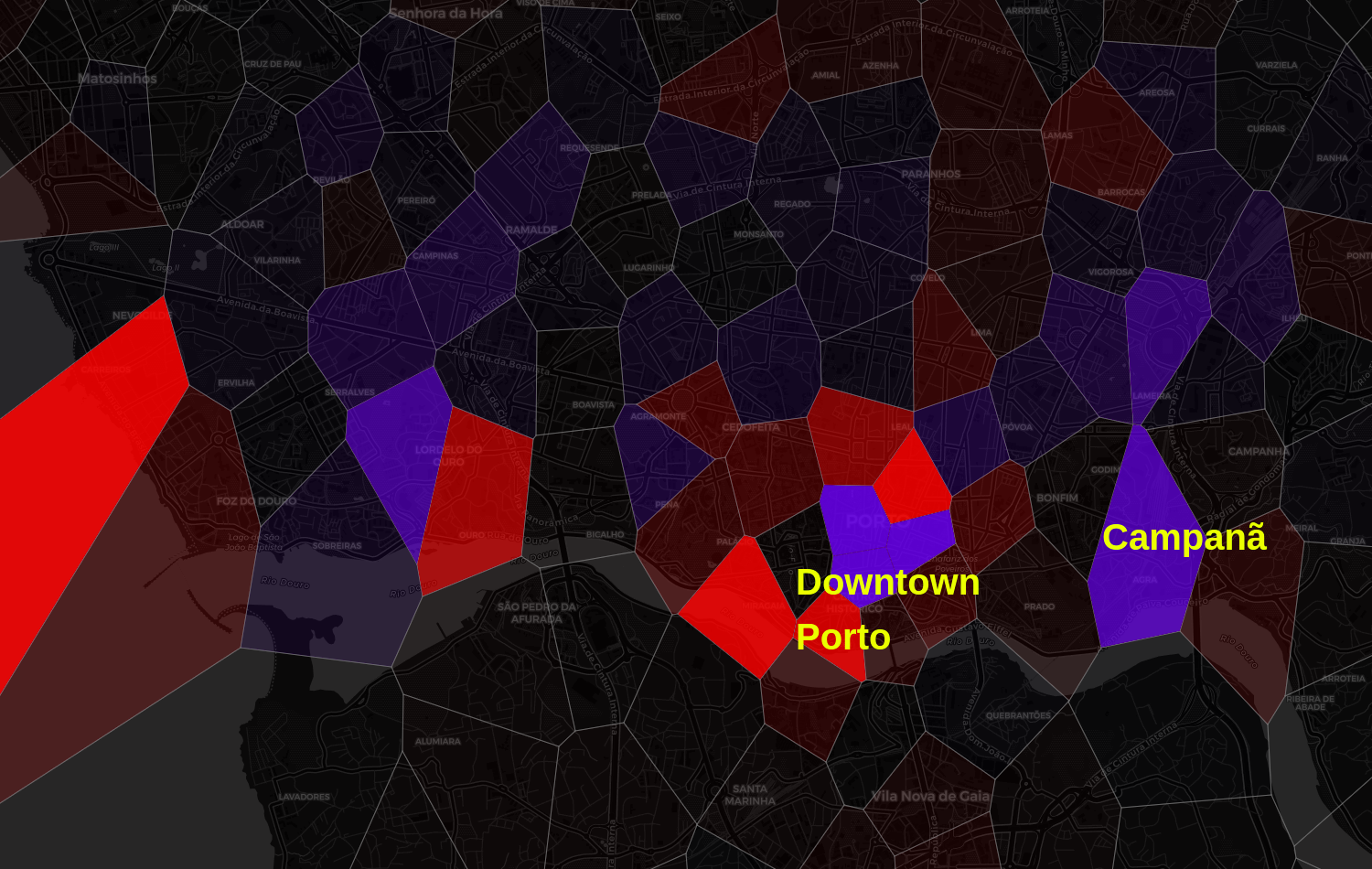
However, there are other drops in June 2014 which we did not anticipate, and which do not coincide with any official holiday. In Fig. 6, we show the results for this region-wise comparison on June 1 and June 6. On June 1 (Fig. 6(a)), we observe a massive surge in activity in a single Voronoi region near Parque Serralves (Serralves Park), a 18-hectare park and part of a local art and cultural institution, Fundação de Serralves (Serralves Foundation). This combined geospatial and temporal localization provides enough contextual clues to research what happened on that date: Serralves em Festa, one of the largest festivals in Europe. The 2014 edition in particular marked the 25th anniversary of the Foundation and the 15th anniversary of its museum, Museu de Serralves, leading to an especially significant celebration (archived at (Fundação de Serralves, 2014) in Portugese).
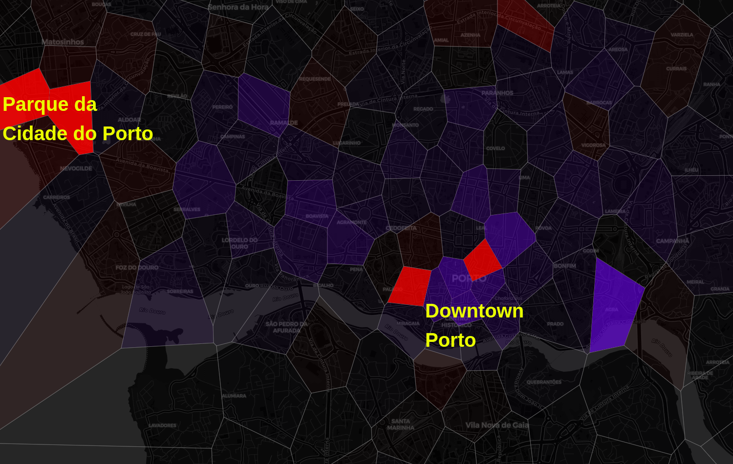
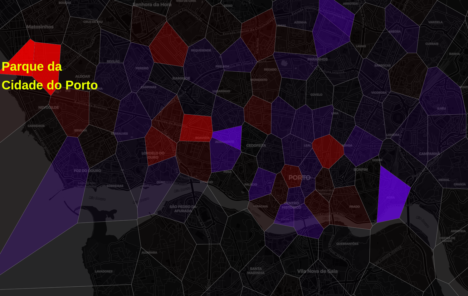
In Fig. 6(b), we show a similar result for June 6, 2014. This anomaly can be traced to an unexpected surge of activity in two adjacent regions comprising Parque da Cidade do Porto (Porto City Park) just south of the beaches of Matosinhos. In fact, researching this date and Parque da Cidade uncovers contemporaneous reports of a major music festival that year, NOS Primavera Sound (archived at (Engenharia Radio, 2014) in Portugese). (Note that the festival takes place June 5–7, but we model taxis originating at regions, and empirically most traffic left the festival after midnight. As a result, the anomalies are detected on June 6–8.)
5.4. Evidence against catastrophic forgetting
Recall that lifelong learning problems such as this one, where knowledge must be acquired incrementally from a data stream, often struggle with catastrophic forgetting: the incorporation of new knowledge degrades information acquired in the past. In that case, the model would need to reacquire its old knowledge by redoing the training process, resulting in a slow increase in mimicking the start of training (Fig. 4, July 2013). However, when anomalies are presented to a well-trained GWR, we observe that instead returns to its high plateau quickly after the cessation of the unusual event (Fig. 4, a–d). This remains true even when the unusual pattern is processed by the network many times in succession. Consider the eight-day Queima das Fitas festival (Fig. 4a): the activity drops suddenly at the beginning of the festival, but returns to a high value immediately afterward. If forgetting had occurred, we would observe a gradual return to higher performance as the model reacquired the lost knowledge.
This follows from two key properties of the GWR update rule (Eqs. 6 and 7). First, updates are only applied to a BMU and its neighbors, , preventing updates from propagating throughout the full network and restricting them to only the most relevant neurons. (The GWR synapse graph tends to be relatively sparse, as visualized for the first-level GWR in Fig. 2(b)). Second, the more often a neuron is activated, the lower its habituation , and thus the smaller its weight update . Therefore, even when weight updates do propagate to a neuron, the network selectively preserves those which are already well-trained.
In Fig. 7 we present additional evidence: one of the last neurons created by the second-level GWR. Repeated anomalies with high activity near Parque da Cidade do Porto (Porto City Park), such as Queima das Fitas (Fig. 5(b)) and the NOS Primavera Sound music festival (Fig. 6(b)) have created a newly-formed neuron, describing a traffic pattern with unusually-high taxi density in these two regions. Once this neuron is created, new inputs with high density in this area (e.g., subsequent days of Queima das Fitas) match most closely with this neuron, making it the BMU and concentrating the weight updates on this neuron (Eqs. 6 and 7). This protects other neurons from a poor weight update, automatically “freezing” their weights until normal traffic behavior resumes, as observed in Fig. 4.
6. Conclusion
The challenges of catastrophic forgetting, concept drift, and model interpretability are difficult open problems in the machine learning community. Where they intersect in the domains of geospatial and transportation modeling, we propose an unsupervised anomaly detector which incrementally learns patterns of life without catastrophic forgetting. These patterns are directly queryable by a human observer at any point in the training process, as are the anomalies themselves, and we show that the detector’s results conform to both known and previously-unreported cultural events in the Porto area. We anticipate that applications of this anomaly detection framework will be of interest to numerous stakeholders with an interest in understanding human mobility patterns, including city governments, urban planners, transportation researchers, and other geospatial professionals.
Acknowledgements.
This work was supported by NGA contract HM0476-21-C-0041. Approved for public release, 22-539.References
- (1)
- Abbar et al. (2020) Sofiane Abbar, Rade Stanojevic, and Mohamed Mokbel. 2020. STAD: Spatio-temporal adjustment of traffic-oblivious travel-time estimation. In 2020 21st IEEE International Conference on Mobile Data Management (MDM). IEEE, 79–88.
- Acevedo-Rodríguez et al. (2011) Javier Acevedo-Rodríguez, Saturnino Maldonado-Bascón, Roberto López-Sastre, Pedro Gil-Jiménez, and Antonio Fernández-Caballero. 2011. Clustering of trajectories in video surveillance using growing neural gas. In International Work-Conference on the Interplay Between Natural and Artificial Computation. Springer, 461–470.
- Andrienko et al. (2011) Gennady Andrienko, Natalia Andrienko, Christophe Hurter, Salvatore Rinzivillo, and Stefan Wrobel. 2011. From movement tracks through events to places: Extracting and characterizing significant places from mobility data. In 2011 IEEE conference on visual analytics science and technology (VAST). IEEE, 161–170.
- Andrienko et al. (2012) Natalia Andrienko, Gennady Andrienko, Hendrik Stange, Thomas Liebig, and Dirk Hecker. 2012. Visual analytics for understanding spatial situations from episodic movement data. KI-Künstliche Intelligenz 26, 3 (2012), 241–251.
- Angelopoulou et al. (2005) Anastassia Angelopoulou, Alexandra Psarrou, José García Rodríguez, and Kenneth Revett. 2005. Automatic landmarking of 2D medical shapes using the growing neural gas network. In International Workshop on Computer Vision for Biomedical Image Applications. Springer, 210–219.
- Ashbrook and Starner (2003) Daniel Ashbrook and Thad Starner. 2003. Using GPS to learn significant locations and predict movement across multiple users. Personal and Ubiquitous computing 7, 5 (2003), 275–286.
- Barbosa et al. (2018) Hugo Barbosa, Marc Barthelemy, Gourab Ghoshal, Charlotte R James, Maxime Lenormand, Thomas Louail, Ronaldo Menezes, José J Ramasco, Filippo Simini, and Marcello Tomasini. 2018. Human mobility: Models and applications. Physics Reports 734 (2018), 1–74.
- Barros et al. (2019) Pablo Barros, German Parisi, and Stefan Wermter. 2019. A personalized affective memory model for improving emotion recognition. In International Conference on Machine Learning. PMLR, 485–494.
- Bauer and Villmann (1997) H-U Bauer and Thomas Villmann. 1997. Growing a hypercubical output space in a self-organizing feature map. IEEE transactions on neural networks 8, 2 (1997), 218–226.
- Beura et al. (2018) Sambit Kumar Beura, Veera Leela Manusha, Haritha Chellapilla, and Prasanta Kumar Bhuyan. 2018. Defining Bicycle Levels of Service Criteria Using Levenberg–Marquardt and Self-organizing Map Algorithms. Transportation in developing economies 4, 2 (2018), 1–11.
- Bracciale et al. (2014) Lorenzo Bracciale, Marco Bonola, Pierpaolo Loreti, Giuseppe Bianchi, Raul Amici, and Antonello Rabuffi. 2014. CRAWDAD dataset roma/taxi (v. 2014-07-17). Downloaded from https://crawdad.org/roma/taxi/20140717. https://doi.org/10.15783/C7QC7M
- Cao et al. (2010) Xin Cao, Gao Cong, and Christian S Jensen. 2010. Mining significant semantic locations from GPS data. Proceedings of the VLDB Endowment 3, 1-2 (2010), 1009–1020.
- Chaudhry et al. (2019) Arslan Chaudhry, Marcus Rohrbach, Mohamed Elhoseiny, Thalaiyasingam Ajanthan, Puneet K Dokania, Philip HS Torr, and Marc’Aurelio Ranzato. 2019. On tiny episodic memories in continual learning. arXiv preprint arXiv:1902.10486 (2019).
- Contreras-Cruz et al. (2019) Marco Antonio Contreras-Cruz, Juan Pablo Ramirez-Paredes, Uriel Haile Hernandez-Belmonte, and Victor Ayala-Ramirez. 2019. Vision-Based Novelty Detection Using Deep Features and Evolved Novelty Filters for Specific Robotic Exploration and Inspection Tasks. Sensors 19, 13 (2019), 2965.
- Das et al. (2019) Soumi Das, Rajath Nandan Kalava, Kolli Kiran Kumar, Akhil Kandregula, Kalpam Suhaas, Sourangshu Bhattacharya, and Niloy Ganguly. 2019. Map enhanced route travel time prediction using deep neural networks. arXiv preprint arXiv:1911.02623 (2019).
- De Brébisson et al. (2015) Alexandre De Brébisson, Étienne Simon, Alex Auvolat, Pascal Vincent, and Yoshua Bengio. 2015. Artificial neural networks applied to taxi destination prediction. In Proceedings of the 2015th International Conference on ECML PKDD Discovery Challenge-Volume 1526. 40–51.
- de Oliveira Martins et al. (2009) Leonardo de Oliveira Martins, Aristófanes Corrêa Silva, Anselmo Cardoso De Paiva, and Marcelo Gattass. 2009. Detection of breast masses in mammogram images using growing neural gas algorithm and Ripley’s K function. Journal of Signal Processing Systems 55, 1 (2009), 77–90.
- Deb and Basu (2015) Budhaditya Deb and Prithwish Basu. 2015. Discovering latent semantic structure in human mobility traces. In European Conference on Wireless Sensor Networks. Springer, 84–103.
- Decker (2005) Reinhold Decker. 2005. Market basket analysis by means of a growing neural network. The International Review of Retail, Distribution and Consumer Research 15, 2 (2005), 151–169.
- Draelos et al. (2017) Timothy J Draelos, Nadine E Miner, Christopher C Lamb, Jonathan A Cox, Craig M Vineyard, Kristofor D Carlson, William M Severa, Conrad D James, and James B Aimone. 2017. Neurogenesis deep learning: Extending deep networks to accommodate new classes. In 2017 International Joint Conference on Neural Networks (IJCNN). IEEE, 526–533.
- Duczek et al. (2021) Nicolas Duczek, Matthias Kerzel, and Stefan Wermter. 2021. Continual Learning from Synthetic Data for a Humanoid Exercise Robot. arXiv preprint arXiv:2102.10034 (2021).
- Ebel et al. (2020) Patrick Ebel, Ibrahim Emre Göl, Christoph Lingenfelder, and Andreas Vogelsang. 2020. Destination prediction based on partial trajectory data. In 2020 IEEE Intelligent Vehicles Symposium (IV). IEEE, 1149–1155.
- Engenharia Radio (2014) Engenharia Radio. 2014. NOS Primavera Sound 2014 (Cartaz e horários) - Engenharia Radio. https://web.archive.org/web/20210902144729/https://www.engenhariaradio.pt/2014/05/nos-primavera-sound-2014-cartaz-e-horarios/.
- Ezenkwu and Starkey (2019) Chinedu Pascal Ezenkwu and Andrew Starkey. 2019. Unsupervised temporospatial neural architecture for sensorimotor map learning. IEEE Transactions on Cognitive and Developmental Systems (2019).
- Farrahi and Gatica-Perez (2011) Katayoun Farrahi and Daniel Gatica-Perez. 2011. Discovering routines from large-scale human locations using probabilistic topic models. ACM Transactions on Intelligent Systems and Technology (TIST) 2, 1 (2011), 1–27.
- Fritzke et al. (1995) Bernd Fritzke et al. 1995. A growing neural gas network learns topologies. Advances in neural information processing systems 7 (1995), 625–632.
- Fu and Lee (2019) Tao-yang Fu and Wang-Chien Lee. 2019. DeepIST: Deep image-based spatio-temporal network for travel time estimation. In Proceedings of the 28th ACM International Conference on Information and Knowledge Management. 69–78.
- Fundação de Serralves (2014) Fundação de Serralves. 2014. Fundação de Serralves - Serralves. https://web.archive.org/web/20140525014007/http://www.serralves.pt/pt/actividades/serralves-em-festa-2014/.
- Gao et al. (2019) Qiang Gao, Fan Zhou, Goce Trajcevski, Kunpeng Zhang, Ting Zhong, and Fengli Zhang. 2019. Predicting human mobility via variational attention. In The World Wide Web Conference. 2750–2756.
- Gupta et al. (2018) Bharat Gupta, Shivam Awasthi, Rudraksha Gupta, Likhama Ram, Pramod Kumar, Bakshi Rohit Prasad, and Sonali Agarwal. 2018. Taxi travel time prediction using ensemble-based random forest and gradient boosting model. In Advances in Big Data and Cloud Computing. Springer, 63–78.
- Hartline (1938) Haldan Keffer Hartline. 1938. The response of single optic nerve fibers of the vertebrate eye to illumination of the retina. American Journal of Physiology-Legacy Content 121, 2 (1938), 400–415.
- Hoch (2015) Thomas Hoch. 2015. An Ensemble Learning Approach for the Kaggle Taxi Travel Time Prediction Challenge.. In DC@ PKDD/ECML.
- Hubel and Wiesel (1974) David H Hubel and Torsten N Wiesel. 1974. Uniformity of monkey striate cortex: a parallel relationship between field size, scatter, and magnification factor. Journal of Comparative Neurology 158, 3 (1974), 295–305.
- Irvine et al. (2018) John M Irvine, Laura Mariano, and Teal Guidici. 2018. Normalcy modeling using a dictionary of activities learned from motion imagery tracking data. In 2018 IEEE Applied Imagery Pattern Recognition Workshop (AIPR). IEEE, 1–9.
- Isele and Cosgun (2018) David Isele and Akansel Cosgun. 2018. Selective experience replay for lifelong learning. In Proceedings of the AAAI Conference on Artificial Intelligence, Vol. 32.
- Jenkins et al. (2019) Porter Jenkins, Ahmad Farag, Suhang Wang, and Zhenhui Li. 2019. Unsupervised representation learning of spatial data via multimodal embedding. In Proceedings of the 28th ACM international conference on information and knowledge management. 1993–2002.
- Jun and Duckett (2003) Li Jun and Tom Duckett. 2003. Robot behavior learning with a dynamically adaptive RBF network: Experiments in offline and online learning. In Proc. 2 Intern. Conf. on Comput. Intelligence, Robotics and Autonomous System, CIRAS. Citeseer.
- Keane (2017) Kevin R Keane. 2017. Detecting motion anomalies. In Proceedings of the 8th ACM SIGSPATIAL Workshop on GeoStreaming. 21–28.
- Kim et al. (2020) Chris Dongjoo Kim, Jinseo Jeong, and Gunhee Kim. 2020. Imbalanced continual learning with partitioning reservoir sampling. In European Conference on Computer Vision. Springer, 411–428.
- Kirkpatrick et al. (2017) James Kirkpatrick, Razvan Pascanu, Neil Rabinowitz, Joel Veness, Guillaume Desjardins, Andrei A Rusu, Kieran Milan, John Quan, Tiago Ramalho, Agnieszka Grabska-Barwinska, et al. 2017. Overcoming catastrophic forgetting in neural networks. Proceedings of the national academy of sciences 114, 13 (2017), 3521–3526.
- Kohonen (1982) Teuvo Kohonen. 1982. Self-organized formation of topologically correct feature maps. Biological cybernetics 43, 1 (1982), 59–69.
- Lam (2016) Hoang Thanh Lam. 2016. A concise summary of spatial anomalies and its application in efficient real-time driving behaviour monitoring. In Proceedings of the 24th ACM SIGSPATIAL International Conference on Advances in Geographic Information Systems. 1–9.
- Lan et al. (2019) Wuwei Lan, Yanyan Xu, and Bin Zhao. 2019. Travel time estimation without road networks: an urban morphological layout representation approach. In Proceedings of the 28th International Joint Conference on Artificial Intelligence. 1772–1778.
- Le Quy et al. (2019) Tai Le Quy, Wolfgang Nejdl, Myra Spiliopoulou, and Eirini Ntoutsi. 2019. A neighborhood-augmented LSTM model for taxi-passenger demand prediction. In International Workshop on Multiple-Aspect Analysis of Semantic Trajectories. Springer, 100–116.
- Lee et al. (2007) Jae-Gil Lee, Jiawei Han, and Kyu-Young Whang. 2007. Trajectory clustering: a partition-and-group framework. In Proceedings of the 2007 ACM SIGMOD international conference on Management of data. 593–604.
- Li et al. (2020) Yadong Li, Bailong Liu, Lei Zhang, Susong Yang, Changxing Shao, and Dan Son. 2020. Fast Trajectory Prediction Method With Attention Enhanced SRU. IEEE Access 8 (2020), 206614–206621.
- Li and Hoiem (2017) Zhizhong Li and Derek Hoiem. 2017. Learning without forgetting. IEEE transactions on pattern analysis and machine intelligence 40, 12 (2017), 2935–2947.
- Liao et al. (2021) Chengwu Liao, Chao Chen, Chaocan Xiang, Hongyu Huang, Hong Xie, and Songtao Guo. 2021. Taxi-Passenger’s Destination Prediction via GPS Embedding and Attention-Based BiLSTM Model. IEEE Transactions on Intelligent Transportation Systems (2021).
- Lin et al. (2013) Miao Lin, Wen-Jing Hsu, and Zhuo Qi Lee. 2013. Detecting modes of transport from unlabelled positioning sensor data. Journal of Location Based Services 7, 4 (2013), 272–290.
- Liu et al. (2020) Yiding Liu, Kaiqi Zhao, Gao Cong, and Zhifeng Bao. 2020. Online anomalous trajectory detection with deep generative sequence modeling. In 2020 IEEE 36th International Conference on Data Engineering (ICDE). IEEE, 949–960.
- Lopez et al. (2017) Clélia Lopez, Panchamy Krishnakumari, Ludovic Leclercq, Nicolas Chiabaut, and Hans Van Lint. 2017. Spatiotemporal partitioning of transportation network using travel time data. Transportation Research Record 2623, 1 (2017), 98–107.
- Marsland et al. (2005) Stephen Marsland, Ulrich Nehmzow, and Jonathan Shapiro. 2005. On-line novelty detection for autonomous mobile robots. Robotics and Autonomous Systems 51, 2-3 (2005), 191–206.
- Marsland et al. (2002) Stephen Marsland, Jonathan Shapiro, and Ulrich Nehmzow. 2002. A self-organising network that grows when required. Neural networks 15, 8-9 (2002), 1041–1058.
- Martinetz and Schulten (1991) Thomas Martinetz and Klaus Schulten. 1991. A “neural-gas” network learns topologies. Artificial neural networks (1991), 397–402.
- McCloskey and Cohen (1989) Michael McCloskey and Neal J Cohen. 1989. Catastrophic interference in connectionist networks: The sequential learning problem. In Psychology of learning and motivation. Vol. 24. Elsevier, 109–165.
- Mici et al. (2018) Luiza Mici, German I Parisi, and Stefan Wermter. 2018. A self-organizing neural network architecture for learning human-object interactions. Neurocomputing 307 (2018), 14–24.
- Moreira-Matias et al. (2013) Luis Moreira-Matias, Joao Gama, Michel Ferreira, Joao Mendes-Moreira, and Luis Damas. 2013. Predicting taxi–passenger demand using streaming data. IEEE Transactions on Intelligent Transportation Systems 14, 3 (2013), 1393–1402.
- Nanni and Pedreschi (2006) Mirco Nanni and Dino Pedreschi. 2006. Time-focused clustering of trajectories of moving objects. Journal of Intelligent Information Systems 27, 3 (2006), 267–289.
- Nehmzow et al. (2013) Ulrich Nehmzow, Yiannis Gatsoulis, Emmett Kerr, Joan Condell, Nazmul Siddique, and T Martin McGuinnity. 2013. Novelty detection as an intrinsic motivation for cumulative learning robots. Intrinsically Motivated Learning in Natural and Artificial Systems (2013), 185–207.
- Neto and Nehmzow (2007) Hugo Vieira Neto and Ulrich Nehmzow. 2007. Visual novelty detection with automatic scale selection. Robotics and Autonomous Systems 55, 9 (2007), 693–701.
- Netto et al. (2012) Stelmo Magalhães Barros Netto, Aristófanes Corrêa Silva, Rodolfo Acatauassú Nunes, and Marcelo Gattass. 2012. Automatic segmentation of lung nodules with growing neural gas and support vector machine. Computers in biology and medicine 42, 11 (2012), 1110–1121.
- News Porto. (2018) News Porto. 2018. Academic tradition at Avenida dos Aliados with students’ parade - News Porto. https://web.archive.org/web/20211201183146/https://www.porto.pt/en/news/academic_tradition_at_avenida_dos_aliados_with_students_parade.
- NYC Taxi & Limousine Commission (nd) NYC Taxi & Limousine Commission. n.d.. TLC Trip Record Data. https://www1.nyc.gov/site/tlc/about/tlc-trip-record-data.page.
- Parisi et al. (2019) German I Parisi, Ronald Kemker, Jose L Part, Christopher Kanan, and Stefan Wermter. 2019. Continual lifelong learning with neural networks: A review. Neural Networks 113 (2019), 54–71.
- Parisi et al. (2017) German I Parisi, Jun Tani, Cornelius Weber, and Stefan Wermter. 2017. Lifelong learning of human actions with deep neural network self-organization. Neural Networks 96 (2017), 137–149.
- Parisi et al. (2018) German I Parisi, Jun Tani, Cornelius Weber, and Stefan Wermter. 2018. Lifelong learning of spatiotemporal representations with dual-memory recurrent self-organization. Frontiers in neurorobotics 12 (2018), 78.
- Pelekis et al. (2009) Nikos Pelekis, Ioannis Kopanakis, Evangelos Kotsifakos, Elias Frentzos, and Yannis Theodoridis. 2009. Clustering trajectories of moving objects in an uncertain world. In 2009 Ninth IEEE international conference on data mining. IEEE, 417–427.
- Piorkowski et al. (2009) Michal Piorkowski, Natasa Sarafijanovic-Djukic, and Matthias Grossglauser. 2009. CRAWDAD dataset epfl/mobility (v. 2009-02-24). Downloaded from https://crawdad.org/epfl/mobility/20090224. https://doi.org/10.15783/C7J010
- Pitonakova and Bullock (2020) Lenka Pitonakova and Seth Bullock. 2020. The robustness-fidelity trade-off in Grow When Required neural networks performing continuous novelty detection. Neural Networks 122 (2020), 183–195.
- Prudent and Ennaji (2005) Yann Prudent and Abdellatif Ennaji. 2005. An incremental growing neural gas learns topologies. In Proceedings. 2005 IEEE International Joint Conference on Neural Networks, 2005., Vol. 2. IEEE, 1211–1216.
- Ransom-Hogg and Spillmann (1980) Anne Ransom-Hogg and Lothar Spillmann. 1980. Perceptive field size in fovea and periphery of the light-and dark-adapted retina. Vision Research 20, 3 (1980), 221–228.
- Ratcliff (1990) Roger Ratcliff. 1990. Connectionist models of recognition memory: constraints imposed by learning and forgetting functions. Psychological review 97, 2 (1990), 285.
- Reades et al. (2007) Jonathan Reades, Francesco Calabrese, Andres Sevtsuk, and Carlo Ratti. 2007. Cellular census: Explorations in urban data collection. IEEE Pervasive computing 6, 3 (2007), 30–38.
- Riemer et al. (2019) Matthew Riemer, Tim Klinger, Djallel Bouneffouf, and Michele Franceschini. 2019. Scalable recollections for continual lifelong learning. In Proceedings of the AAAI Conference on Artificial Intelligence, Vol. 33. 1352–1359.
- Rodrigues et al. (2020) Pedro Rodrigues, Ana Martins, Sofia Kalakou, and Filipe Moura. 2020. Spatiotemporal variation of taxi demand. Transportation Research Procedia 47 (2020), 664–671.
- Rösler and Liebig (2013) Roberto Rösler and Thomas Liebig. 2013. Using data from location based social networks for urban activity clustering. In Geographic information science at the heart of Europe. Springer, 55–72.
- Rossi et al. (2019) Alberto Rossi, Gianni Barlacchi, Monica Bianchini, and Bruno Lepri. 2019. Modelling taxi drivers’ behaviour for the next destination prediction. IEEE Transactions on Intelligent Transportation Systems 21, 7 (2019), 2980–2989.
- Rudloff and Ray (2010) Christian Rudloff and Markus Ray. 2010. Detecting travel modes and profiling commuter habits solely based on GPS data. Technical Report.
- Rusu et al. (2016) Andrei A Rusu, Neil C Rabinowitz, Guillaume Desjardins, Hubert Soyer, James Kirkpatrick, Koray Kavukcuoglu, Razvan Pascanu, and Raia Hadsell. 2016. Progressive neural networks. arXiv preprint arXiv:1606.04671 (2016).
- Saadallah et al. (2018) Amal Saadallah, Luis Moreira-Matias, Ricardo Sousa, Jihed Khiari, Erik Jenelius, and Joao Gama. 2018. BRIGHT—drift-aware demand predictions for taxi networks. IEEE Transactions on Knowledge and Data Engineering 32, 2 (2018), 234–245.
- Song et al. (2018) Li Song, Ruijia Wang, Ding Xiao, Xiaotian Han, Yanan Cai, and Chuan Shi. 2018. Anomalous trajectory detection using recurrent neural network. In International Conference on Advanced Data Mining and Applications. Springer, 263–277.
- Spillmann (2014) Lothar Spillmann. 2014. Receptive fields of visual neurons: the early years. Perception 43, 11 (2014), 1145–1176.
- Stanley (1976) James C Stanley. 1976. Computer simulation of a model of habituation. Nature 261, 5556 (1976), 146–148.
- Sun et al. (2017) Qianru Sun, Hong Liu, and Tatsuya Harada. 2017. Online growing neural gas for anomaly detection in changing surveillance scenes. Pattern Recognition 64 (2017), 187–201.
- Toch et al. (2019) Eran Toch, Boaz Lerner, Eyal Ben-Zion, and Irad Ben-Gal. 2019. Analyzing large-scale human mobility data: a survey of machine learning methods and applications. Knowledge and Information Systems 58, 3 (2019), 501–523.
- Todorov et al. (2020) Helena Todorov, Robrecht Cannoodt, Wouter Saelens, and Yvan Saeys. 2020. TinGa: fast and flexible trajectory inference with Growing Neural Gas. Bioinformatics 36, Supplement_1 (2020), i66–i74.
- Visitar Porto (nda) Visitar Porto. n.d.a. Festival of São João do Porto, Portugal. https://web.archive.org/web/20211030040838/https://www.visitar-porto.com/en/whats-on/porto-events/festa-de-sao-joao.html.
- Visitar Porto (ndb) Visitar Porto. n.d.b. Queima das Fitas (Burning of the Ribbons) Porto, Portugal. https://web.archive.org/web/20210506221158/https://www.visitar-porto.com/en/whats-on/porto-events/porto-queima-das-fitas.html,.
- Watson et al. (2020) James R Watson, Zach Gelbaum, Mathew Titus, Grant Zoch, and David Wrathall. 2020. Identifying multiscale spatio-temporal patterns in human mobility using manifold learning. PeerJ Computer Science 6 (2020), e276.
- Wu et al. (2017) Hao Wu, Weiwei Sun, and Baihua Zheng. 2017. A fast trajectory outlier detection approach via driving behavior modeling. In Proceedings of the 2017 ACM on Conference on Information and Knowledge Management. 837–846.
- Xiao et al. (2014) Tianjun Xiao, Jiaxing Zhang, Kuiyuan Yang, Yuxin Peng, and Zheng Zhang. 2014. Error-driven incremental learning in deep convolutional neural network for large-scale image classification. In Proceedings of the 22nd ACM international conference on Multimedia. 177–186.
- Ying et al. (2014) Josh Jia-Ching Ying, Wang-Chien Lee, and Vincent S Tseng. 2014. Mining geographic-temporal-semantic patterns in trajectories for location prediction. ACM Transactions on Intelligent Systems and Technology (TIST) 5, 1 (2014), 1–33.
- Yoon et al. (2018) Jaehong Yoon, Eunho Yang, Jeongtae Lee, and Sung Ju Hwang. 2018. Lifelong Learning with Dynamically Expandable Networks. In International Conference on Learning Representations.
- Yuan et al. (2010) Jing Yuan, Yu Zheng, Chengyang Zhang, Wenlei Xie, Xing Xie, Guangzhong Sun, and Yan Huang. 2010. T-Drive: Driving Directions Based on Taxi Trajectories. In Proceedings of 18th ACM SIGSPATIAL Conference on Advances in Geographical Information Systems (proceedings of 18th acm sigspatial conference on advances in geographical information systems ed.). ACM SIGSPATIAL GIS 2010. https://www.microsoft.com/en-us/research/publication/t-drive-driving-directions-based-on-taxi-trajectories/ Best Paper Award.
- Zenke et al. (2017) Friedemann Zenke, Ben Poole, and Surya Ganguli. 2017. Continual learning through synaptic intelligence. In International Conference on Machine Learning. PMLR, 3987–3995.
- Zhang et al. (2018) Lei Zhang, Guoxing Zhang, Zhizheng Liang, and Ekene Frank Ozioko. 2018. Multi-features taxi destination prediction with frequency domain processing. PloS one 13, 3 (2018), e0194629.
- Zhang et al. (2019) Xiaocai Zhang, Zhixun Zhao, Yi Zheng, and Jinyan Li. 2019. Prediction of taxi destinations using a novel data embedding method and ensemble learning. IEEE Transactions on Intelligent Transportation Systems 21, 1 (2019), 68–78.
- Zhou et al. (2012) Guanyu Zhou, Kihyuk Sohn, and Honglak Lee. 2012. Online incremental feature learning with denoising autoencoders. In Artificial intelligence and statistics. PMLR, 1453–1461.
- Zion and Lerner (2017) Eyal Ben Zion and Boaz Lerner. 2017. Learning human behaviors and lifestyle by capturing temporal relations in mobility patterns.. In ESANN.
Appendix A Appendix
GWR illustration on toy problem
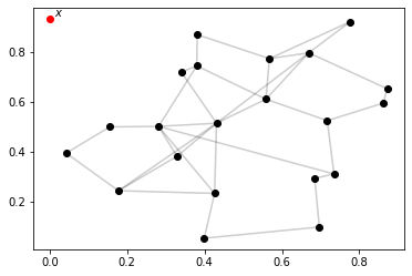
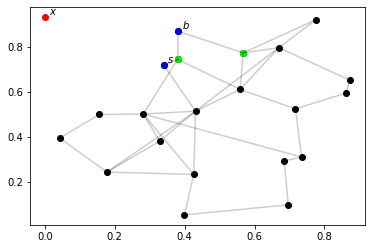
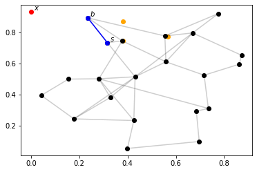
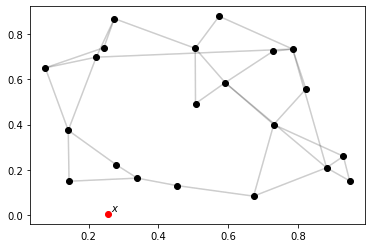
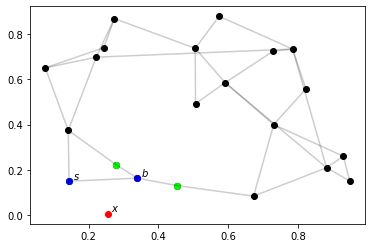
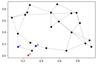
To provide a geometric intuition and visual illustration of the GWR algorithm, as outlined in the main text, we include Figs. 8 and 9 here. We illustrate the algorithm on a toy problem, using random samples from a two-dimensional uniform distribution with increased learning rates to better highlight the model’s behavior in each iteration.
Figure Fig. 8 demonstrates, at a high level, the GWR’s behavior during a weight update (Section 4.2.5). Figure Fig. 9 demonstrates, at a high level, the GWR’s behavior during neurogenesis (Section 4.2.4).
First-level GWR (regions)
Note that these hyperparameters are largely the same as in previous work, although with different notational convention (Parisi et al., 2017, 2018). We make only narrow changes. First, we alter the activity threshold to only add neurons when no existing neuron is closer than 1 km. Second, we reduce the habituation rates to slow neurogenesis due to the immense number of trajectories (over 1 million) to be processed. Third, and finally, we disable neuron death (the removal of a neuron if ), because removing a neuron from the first-level GWR removes a learned region, deleting information from the second-level GWR that is essential for city-wide anomaly detection (Fig. 3). At the end of training, this GWR contains 531 neurons total, each representing a region of Porto or the surrounding area.
Hyperparameter values
| threshold for neurogenesis | ||
| threshold for neurogenesis | ||
| learning rate (BMU) | ||
| learning rate (neighbors) | ||
| controls habituation | ||
| controls habituation (BMU) | ||
| controls habituation (neighbors) | ||
| threshold for synapse pruning |
Second-level GWR (city-wide patterns)
The second-level GWR uses values previously published in the literature (Parisi et al., 2017, 2018) for all hyperparameters except , which we set to 1. As a result, neurogenesis is limited only by habituation , not by the activity , encouraging the formation of more neurons. At the end of training, this GWR contains 69 neurons total, each representing a prototypical traffic pattern throughout Porto’s regions.
Hyperparameter values
| threshold for neurogenesis | ||
| threshold for neurogenesis | ||
| learning rate (BMU) | ||
| learning rate (neighbors) | ||
| controls habituation | ||
| controls habituation (BMU) | ||
| controls habituation (neighbors) | ||
| threshold for synapse pruning |