Ground-based observability of Dimorphos DART impact ejecta: Photometric predictions

Abstract

The Double Asteroid Redirection Test (DART) is a NASA mission intended to crash a projectile on Dimorphos, the secondary component of the binary (65803) Didymos system, to study its orbit deflection. As a consequence of the impact, a dust cloud will be be ejected from the body, potentially forming a transient coma- or comet-like tail on the hours or days following the impact, which might be observed using ground-based instrumentation. Based on the mass and speed of the impactor, and using known scaling laws, the total mass ejected can be roughly estimated. Then, with the aim to provide approximate expected brightness levels of the coma and tail extent and morphology, we have propagated the orbits of the particles ejected by integrating their equation of motion, and have used a Monte Carlo approach to study the evolution of the coma and tail brightness. For typical power-law particle size distribution of index –3.5, with radii r_rmin=1 $\mu$m and r_max=1 cm, and ejection speeds near 10 times the escape velocity of Dimorphos, we predict an increase of brightness of $\sim$3 magnitudes right after the impact, and a decay to pre-impact levels some 10 days after. That would be the case if the prevailing ejection mechanism comes from the impact-induced seismic wave. However, if most of the ejecta is released at speeds of the order of $\gtrsim$100 $\mathrm{m\;s^{-1}}$, the observability of the event would reduce to a very short time span, of the order of one day or shorter.

1 Introduction

The Double Asteroid Redirection Test (DART) (Cheng et al., 2018) is a planetary defence mission launched November 24th, 2021 by NASA. This mission is aimed to test asteroid-deflecting technology by crashing a $\sim$535 kg projectile on the surface of Dimorphos, a $\sim$160 m diameter body orbiting the larger (780 m) main-belt asteroid (65803) Didymos. During the first few minutes after the impact, the Light Italian CubeSat for Imaging Asteroids, or LICIACube (Dotto et al., 2021), will be taking images of the early ejecta. At the planned collision time (2022 September 26th, 23:14 UT) and the few days following the impact, this binary system will be well placed for southern hemisphere observers, and at fairly high galactic latitudes (–50^∘ to –30^∘ between 2022 September 26, and October 8), so that relatively clear background star fields are foreseen. Ground-based observations of the dust cloud generated after the impact and its evolution with time will provide information on the amount of mass released, the ejection speeds, and the physical properties of the dust particles. In order to estimate some of these parameters in advance, which might aid to plan the observations, we have performed simulations of the evolution of the dust coma and tail that will appear after the impact, its brightness level, extent, and morphology. In section 2 we describe the physical model used, and the governing equation of motion of the ejected particles. In section 3 we describe the method used to integrate the equation of motion, and a comparison with an independent N-body simulator is performed for validation purposes. Section 4 gives a description of the procedure to build up the dust tail synthetic images, along with the particle physical properties adopted and the expected dust mass released. In Section 5, the dust tail code is further validated, for sufficiently high ejection speeds, with our classical Monte Carlo dust tail code that we routinely use to fit cometary and active asteroid tail images (see e.g. Moreno et al., 2021, and references therein). Section 6 shows the results obtained concerning dust tail brightness simulations as well as synthetic lightcurves as a function of the ejecta speed. Finally, the conclusions of this work are given in Section 7.

2 Physical model of the binary system

The DART impact is foreseen to occur on 2022 September 26th, 23:14 UT (JD=2459849.46806). The impactor mass is assumed at $m_{i}$=535 kg, and its speed at impact time, $v_{i}$=6.7 $\mathrm{km\;s^{-1}}$. We assume that the binary components of the asteroid system are both spherical, and adopt physical parameters from the latest ESA’s Hera Mission (Michel et al., 2018) Didymos Reference Model available (12/03/2020, see Table  1). The binary system has a mutual orbit period of $P_{sec}$=11.9217 h and a semi-major axis of $a_{sec}$=1.19 km. Hence, using the Kepler’s third law, the total system mass becomes $M_{T}$=5.4$\times$10¹¹ kg. The Dimorphos mass, assuming the same density as Didymos, will be $M_{sec}$=5$\times$10⁹ kg. The Didymos rotation is retrograde, the north pole of the spin axis pointing to ecliptic coordinates $(\lambda_{e},\beta_{e})$=(320.6^∘,–78.6^∘). This orientation correspond to the latest orbit solution JPL 104 for Dimorphos (Naidu et al., 2021), whose orbit is contained in the Didymos equatorial plane. The heliocentric ecliptic coordinates and velocity of Didymos at the impact time are taken from the JPL Horizons on-line Ephemeris System. The Dimorphos coordinates and velocity components relative to Didymos body centre at impact time are also taken from the JPL Horizons web site. For completeness, these coordinates and velocities are shown in Table  2.

Table 1: Physical parameters for the Didymos-Dimorphos system, adopted from latest Hera Didymos Reference Model available (12/03/2020).

Parameter	Value
Didymos diameter	780$\pm$30 m
Dimorphos diameter	164$\pm$18 m
Semimajor axis of Dimorphos orbit	1.19$\pm$0.03 km
Dimorphos orbital period	11.9217$\pm$0.0002 h
Didymos density	2170$\pm$350 $\mathrm{kg\;m^{-3}}$

Table 2: Heliocentric ecliptic coordinates and velocity at impact time (JD=2459849.46806). The Dimorphos data are relative to Didymos body centre. All coordinates are taken from JLP Horizons on-line Ephemeris System. Units are $\mathrm{au}$ for position and $\mathrm{au\;day^{-1}}$ for velocity components.

Didymos
X=1.040512227512945E+00	Y= 9.017812950063080E-02	Z=-5.774272064726729E-02
$V_{x}$=-4.229184367475531E-03	$V_{y}$=1.917344670139128E-02	$V_{z}$=5.728269981716490E-04
Dimorphos
$\Delta$X=–5.604615661026744E-09	$\Delta$Y=-5.736939008292839E-09	$\Delta$Z=-1.390204184153139E-10
$\Delta V_{x}$=-7.091500670770579E-08	$\Delta V_{y}$=6.976345650818189E-08	$\Delta V_{z}$=-1.997791163791703E-08

The heliocentric position of Didymos at any time during the particle orbital integration is computed from its orbital elements. For Dimorphos, we compute its position relative to Didymos from its orbital elements related to Didymos body centre. The orbit of Dimorphos relative to Didymos becomes elliptical, with a small eccentricity of $\epsilon$=0.04, in line with previous estimates (see e.g. Scheirich & Pravec, 2009; Fang & Margot, 2012; Naidu et al., 2020).

For the particle orbit integration, we use the heliocentric ecliptic coordinate system relative to Didymos body centre, denoted by lowercase letters $(x,y,z)$. We define a colatitude-longitude $(\theta,\phi)$ grid on Dimorphos surface so that the initial position of the particle on Dimorphos is given by: $x_{i}=R_{sec}\cos\phi\sin\theta$, $y_{i}=R_{sec}\sin\phi\sin\theta$, and $z_{i}=R_{sec}\cos\theta$, where $R_{sec}=D_{sec}/2$. The initial coordinates of the particle relative to Didymos are given by:

$$x_{0}=x_{i}+\Delta X$$ (1)

$$y_{0}=y_{i}+\Delta Y$$

$$z_{0}=z_{i}+\Delta Z$$

where ($\Delta$X,$\Delta$Y,$\Delta$Z) are the initial coordinates of Dimorphos relative to Didymos (see Table  2). The heliocentric ecliptic coordinates of the particle are given by:

$$X_{p}=x+X_{D}$$ (2)

$$Y_{p}=y+Y_{D}$$

$$Z_{p}=z+Z_{D}$$

where $(X_{D},Y_{D},Z_{D})$ are the heliocentric coordinates of Didymos.

Another Didymos-centred reference frame is defined as the one having $(\xi,\eta,\zeta)$ axes, where the $\xi$ axis points to the same direction and sense as the Sun-to-Didymos radius vector, $\eta$ is contained in the asteroid orbital plane and is directed opposite to its orbital motion, and $\zeta$ is perpendicular to the orbital plane and chosen to form a right-handed set with $\xi$ and $\eta$ axes (see Finson & Probstein, 1968). This reference frame is useful to build up the dust tail as seen from Earth, by projecting the particle $(\xi,\eta,\zeta)$ coordinates onto the so-called $(N,M)$ photographic plane. The equations giving such projection are given in Finson & Probstein (1968). This transformation also involves the computation of the Earth coordinates at the time of observation $(\xi_{E},\eta_{E},\zeta_{E})$, which are computed from its heliocentric ecliptic coordinates, available in the JPL Horizons on-line Ephemeris System. The transformation of heliocentric ecliptic coordinates to the $(\xi,\eta,\zeta)$ asteroid-centred reference frame is performed by standard methods.

In addition to the gravity forces from the bodies involved, the only non-gravitational force acting on a particle that we consider in the model is the solar radiation pressure. Thus, the Poynting-Robertson drag on the particles is only important in very long-term dynamics, and is therefore neglected. The Lorentz acceleration, that would act on the smallest grains of the assumed size distribution, can be written as (Price et al., 2019):

$$a_{L}=\frac{12\epsilon_{0}V_{P}}{C^{2}}\beta^{2}\frac{\rho_{p}}{Q_{pr}^{2}}B_{\phi}V_{sw}$$ (3)

where $\epsilon_{0}$ is the vacuum permittivity, $V_{P}$ is the potential on the grain surface, assumed here as $V_{P}$=+5 V (Mukai, 1981; Grün et al., 1994), $C$=5.76$\times$10^-4 $\mathrm{kg\;m^{-2}}$, $\rho_{p}$ is the particle density, assumed at having the same value as the bulk density of the asteroid, $Q_{pr}$ is the scattering efficiency for radiation pressure, which takes the value $Q_{pr}$=1, $B_{\phi}$ is the azimuthal component of the interplanetary magnetic field, which has a mean value of $B_{\phi}$=3 nT at 1 au from the Sun (Landgraf, 2000), and $V_{sw}$ is the solar wind speed, which is taken as 400 $\mathrm{km\;s^{-1}}$ (Grün et al., 1994). The quantity $\beta$ is defined as the ratio of radiation pressure force to gravity force, as $\beta=F_{rad}/F_{grav}=C_{pr}Q_{pr}/(2\rho_{p}a_{p})$, where $C_{pr}$=1.19$\times$ 10^-3 kg m^-2, and $a_{p}$ is the grain radius. For the Lorentz acceleration, we then obtain $a_{L}=0.004\beta^{2}$ $\mathrm{m\;s^{-2}}$. The radiation pressure force is given by $a_{RP}=(1-\beta)GM_{\odot}/r_{h}^{2}$, where $G$ is the gravitational constant, $M_{\odot}$ is the Sun mass, and $r_{h}$ is the heliocentric distance of the grain. At $r_{h}$= 1 au, we have $a_{RP}=0.006(1-\beta)$ $\mathrm{m\;s^{-2}}$. Therefore, at the lower limit of the size distribution ($a_{p}$=1 $\mu$m, see section 4), $a_{RP}$ is higher than $a_{L}$ in more than an order of magnitude. The ratio $a_{RP}/a_{L}$ increases as $\beta$ decreases, or, equivalently, $a_{p}$ increases. We then neglect the Lorentz force in our approach. Hence, the equation governing the trajectory of each individual grain can be written as:

$$\frac{d^{2}\mathbf{r_{d}}}{dt^{2}}= W_{1}\frac{\mathbf{r_{d}}}{r_{d}^{3}}+W_{2}\frac{\mathbf{r_{d}}-\mathbf{r_{s}}}{\|\mathbf{r_{d}}-\mathbf{r_{s}}\|^{3}}+W_{3}\left[\frac{\mathbf{r_{s}}-\mathbf{r_{d}}}{\|\mathbf{r_{s}}-\mathbf{r_{d}}\|^{3}}-\frac{\mathbf{r_{s}}}{r_{s}^{3}}\right]+$$ (4)

$$W_{4}\left[\frac{\mathbf{r_{dsec}}}{r_{dsec}^{3}}-\frac{\mathbf{r_{sec}}}{r_{sec}^{3}}\right]$$

where $\mathbf{r_{d}}$ is the Didymos-to-dust grain vector, $\mathbf{r_{s}}$ is the Didymos-to-Sun vector, $\mathbf{r_{dsec}}$ is the vector from the dust grain to Dimorphos, and $\mathbf{r_{sec}}$ is the Didymos-to-Dimorphos vector. We have used the fact that $\mathbf{r_{s}}$=$\mathbf{r_{d}}$ + $\mathbf{r_{ds}}$, where $\mathbf{r_{ds}}$ is the vector from the dust grain to the Sun. Figure  1 provides a schematic drawing of the vectors used. The other terms are $W_{1}=-GM_{P}$, $W_{3}=GM_{\odot}$ ($M_{P}$ is Didymos mass), and $W_{4}=GM_{sec}$. The remaining term, $W_{2}$, is given by:

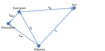
Figure 1: Schematic drawing of the vectors shown in Equation  4.

$$W_{2}=\frac{Q_{pr}}{c}\frac{E_{s}}{4\pi}\frac{\pi d^{2}}{4m_{p}}$$ (5)

In equation  5, $c$ is the speed of light, $E_{s}$=3.93$\times$10²⁶ W is the total power radiated by the Sun, $d$ is the particle diameter ($d$=2$a_{p}$), and $m_{p}$ is the particle mass ($m_{p}=\rho_{p}(4/3)\pi a_{p}^{3}$).

3 Orbital simulations

To compute the trajectory of each particle, equation  4 is integrated numerically following a fourth-order Runge-Kutta (RK4) method. A constant time step of 100 s was found appropriate to conduct the simulations. At each time step, we check whether the particle is within the shadowed region of Didymos, so that the radiation pressure was set to zero in that region. Since the geometrical cross section of Dimorphos is very small, and in order to save computational time, we do not take into account its projected shadow in the calculations. The fate of each particle can be either (1) a collision with Didymos, (2) a collision with Dimorphos, or (3) released to outer space, feeding up the dust coma/tail. Sample trajectories are shown in Figure  2. Small particles tend to leave the binary system very fast, feeding up the tail, while large particles stay orbiting the system for some time, or eventually collide either with Didymos or with Dimorphos.

\begin{overpic}[angle={-90},width=173.44534pt]{orbit1-eps-converted-to.pdf} \put(67.0,89.0){\Large(a)} \end{overpic}	\begin{overpic}[angle={-90},width=173.44534pt]{orbit5-eps-converted-to.pdf} \put(61.0,89.0){\Large(b)} \end{overpic}
\begin{overpic}[angle={-90},width=216.81pt]{orbit2-eps-converted-to.pdf} \put(90.0,85.0){\Large(c)} \end{overpic}	\begin{overpic}[angle={-90},width=216.81pt]{orbit3-eps-converted-to.pdf} \put(90.0,85.0){\Large(d)} \end{overpic}

Figure 2: Sample orbits of $r$=1 cm particles ejected at Dimorphos escape velocity from various locations on Dimorphos surface, projected to the $x-y$ plane, and integrated from impact time to October 2nd, 2022. The initial positions of Didymos (large red filled circle) and Dimorphos (small blue filled circle) are given. The orbits are drawn as green lines. (a) Orbit of a particle which is orbiting the binary asteroid and remains close to the system at the end of the integration. (b) A particle that leaves the system, contributing to the far tail region brightness. (c) A particle colliding with Dimorphos before the end of integration. The position of Dimorphos at the collision time is drawn as a purple circle. (d) A particle that collides with Didymos before the end of integration.

With the purpose of validating the results obtained, we have also performed test simulations using the MERCURY N-body software package for orbital dynamics (Chambers, 1999). In addition to Didymos, Dimorphos, and the corresponding particle, the planets Mercury, Venus, the Earth-Moon system, Mars, and Jupiter were included in the simulations. While the effect of all those planets in the short time integration interval of the ejecta that we provide is minimal, we keep the procedure as it is for future longer-term studies. The radiation pressure force was set by writing a dedicated user-defined force routine in the computer code. A Bulirsch-Stöer integrator was used, with a time step of 10^-3 days (86.4 s), i.e., similar to the 100 s used for the RK4 simulations above. The initial heliocentric ecliptic coordinates and velocities of all the bodies were taken from the JPL Horizons on-line Ephemeris System as described above. The initial heliocentric position and velocity components of Dimorphos and the particle were also set as indicated above, assuming randomly selected radial direction ejection from Dimorphos spherical surface. Figure  3 shows a comparison of the fate of 1 cm particles, on September 28th, 2022, ejected at $v$=0.36 $\mathrm{m\;s^{-1}}$ from Dimorphos surface using both the RK4 and MERCURY procedures, where an excellent agreement can be seen.

Figure 3: Final positions, projected on the x-y planes (panels (a) and (b)) and x-z planes (panels (c) and (d)), relative to Didymos position, on September 28th, 2022, of 10⁴ particle of $r$=1 cm ejected randomly in all directions from Dimorphos at the impact time. The ejection speed is four times the escape velocity of Dimorphos, i.e., $v$=0.36 $\mathrm{m\;s^{-1}}$. Panels (a) and (c) are the results from the RK4 code, and panels (b) and (d) are the corresponding calculations using MERCURY (Chambers, 1999) code.

4 Dust tail build-up

The last step at the end of the orbital integration is the calculation is the projection of the particle position onto the sky $(N,M)$ plane, as described previously. The $(N,M)$ coordinates are finally rotated to equatorial coordinates $(RA,DEC)$ through the asteroid position angle, so that the tail images are provided in the conventional North up, East to left orientation. In this way, they can be directly compared with Earth-based telescope observations.

The brightness of the tail is computed by adding up the contribution of each particle of the large set of particles that are released from Dimorphos surface, taking into account the particle physical properties, the size distribution, and the total dust mass ejected. This procedure has been outlined in many previous papers (see e.g. Moreno et al., 2021, and references therein). For completeness, however, a description of the method is given in the Appendix.

We assume that the physical properties of the particles are in line with the Didymos known properties. A geometric albedo of $p_{R}$=0.16$\pm$0.04 has been estimated for Didymos (Pravec et al., 2006). Then, a linear phase coefficient of $\phi=0.013-0.0104\ln p_{R}$=0.032 $\mathrm{mag\;deg^{-1}}$ is calculated from Shevchenko’s (see Shevchenko, 1997) magnitude-phase relationship. We assume that this applies to both Didymos surface and the ejected particles. On the other hand, as already stated, the density of the particles is assumed to be the same as the bulk density of the asteroid, i.e., $\rho_{p}$=2170 $\mathrm{kg\;m^{-3}}$.

The ejected particles are assumed to be distributed following a differential power-law size distribution function, i.e., $n(r)\propto r^{\kappa}$, where we assume an index $\kappa$=–3.5, and having a broad size range from $a_{p}$=1 $\mu$m to $a_{p}$=1 cm. Those values can be considered as typical for the dust grains ejected from active asteroids (see e.g. Moreno et al., 2019, and references therein). The dust ejection is assumed to proceed instantly at the impact time, i.e., no particle emission is considered afterwards.

The impact will generate a crater on Dimorphos surface, from which the particles will be ejected. This is a primary ejection mechanism, although more complex mechanisms surely will also be playing a role, such as impact-induced seismic waves propagation across the body, which is able to produce lift-off of small particles due to shaking (Tancredi et al., 2022). In the event that this shaking mechanism is dominating the particle ejection, the expected speeds would be of the order of Dimorphos escape speed, and the dust mass released would be comparable to that produced by the impact itself (Tancredi et al., 2022). While a large range of ejection speeds might be expected, the fast moving material will get dispersed very rapidly in space, being difficult to detect, but the low-speed component of the ejecta will contribute to form a detectable dust plume, in a way similar to impacted active asteroids such as (596) Scheila (Jewitt et al., 2011; Moreno et al., 2011). Given the large uncertainty in the relative contribution of those mechanisms (see, e.g. Yu & Michel, 2018), and the speed distribution of the ejecta, we will assume different scenarios and will compute the corresponding coma (by aperture photometry) and tail brightness at different dates following the impact date in an attempt to provide some insight into the detectability of the phenomenon as seen from Earth.

An order-of-magnitude estimate of the ejected mass by the impact is provided by the scaling laws of Housen and Holsapple (see Housen & Holsapple, 2011, their figure 4). For impacts into basalt powder and dry quartz sand, for ejecta speeds of the order of the mean value of the escape speeds of the binary system, ($v_{ej}\sim$0.25 $\mathrm{m\;s^{-1}}$), we get $v_{ej}/v_{i}$=4$\times$10^-5. Then, the ratio of the mass ejected with speeds higher than $v_{ej}$, $M_{ej}$, to the impactor mass is $M_{ej}/m_{i}\sim$ 9000, so that $M_{ej}\sim$ 5$\times$10⁶ kg. This assumes that the impactor and the target have the same bulk density, so it must be considered as an order-of-magnitude approximation. For comparison, the Deep Impact projectile, having $m_{i}$=370 kg and $v_{i}$=10.3 $\mathrm{km\;s^{-1}}$ (and therefore similar momentum to DART impactor) produced a dust cloud around comet 9P/Tempel 1 of 10⁶ kg (Sugita et al., 2005), i.e., the same order of magnitude than assumed here.

The ejection speed distribution is unknown. According to both modelling of impacted asteroids such as (596) Scheila (Moreno et al., 2011) and laboratory collision experiments (Giblin, 1998) there seems to be a weak dependence of particle speed with size. We will assume different ejection speeds starting from the escape velocity of Dimorphos ($v_{esc}$=0.09 $\mathrm{m\;s^{-1}}$). Koschny & Grün (2001), from their impact experiments into ice-silicate surfaces, gave an upper limit to the ejecta speeds of the order of 700-800 $\mathrm{m\;s^{-1}}$, independently of projectile speeds, that we adopt as an upper limit in our computations.

5 Comparison with our Monte Carlo dust tail code

As another check of the calculations, our method was compared with the outcome of the Monte Carlo dust tail code that we routinely use to retrieve the dust environment from active asteroids and comets (see e.g. Moreno et al., 2021, and references therein). In such a code, the only forces considered on particles are the solar gravity and radiation pressure, so that their trajectories around the Sun are Keplerian, and the numerical simulation proceeds way faster than with the detailed trajectory calculations provided here with the integration of the equation of motion  4. For ejection speeds larger than the escape velocity of the binary system the two methods should give similar results, since at such speeds only a small fraction of the ejected mass is delivered to Didymos and Dimorphos, as we will see later (see Table  5), and the gravity forces of the small binary components is not very important. Figure  4 displays a comparison between the two methods, for simulated tails corresponding to a ejection speed of $v$=0.7 $\mathrm{m\;s^{-1}}$, for an observation date of October 2nd, 2022, with the rest of physical parameters as stated above. Agreement is very good between the two methods. Therefore we can trust the new, more accurate, approach. For speeds near the escape velocity of the system or smaller, the comparison is meaningless, as the trajectory of particles would differ, and, besides, a considerable fraction of the ejected mass is actually transferred to the two binary components (see Table  5).

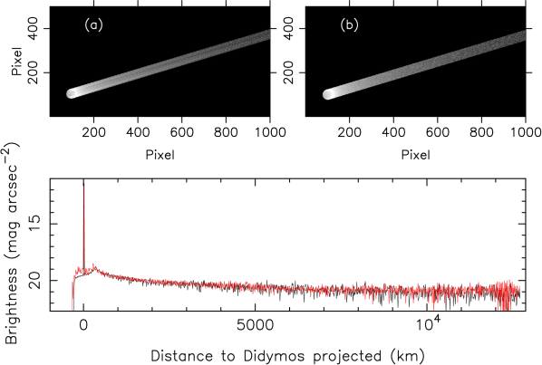
Figure 4: Simulated tail images of the Didymos system as would be seen from Earth after DART impact (Sept. 26.986, 2022) on October 2nd, 2022, with the detailed method consisting on the integration of equation  4 (panel (a)), and the Monte Carlo dust tail code (panel (b)) considering only solar gravity and radiation pressure forces. The lowermost panel depicts a comparison between brightness scans along the tail for images (a) (red line) and (b) (black line), as a function of distance to Didymos projected. The spikes at zero projected distance is caused by the Didymos surface brightness. The orientation of the images is the conventional: celestial North up, East to the left.

6 Results and discussion

6.1 Dust tail simulations

First of all, we generate the synthetic dust tail that, under low-speed ejecta conditions, would be observable from the Earth. Simulations are performed at various observing dates, from one day after the impact up to five days later, at four different ejection speeds namely the Dimorphos escape velocity, and twice, four, and eight times that value. Table  3 shows the assumed circumstances for the three dates. The plate scale in $\mathrm{km\;px^{-1}}$ of the last column has been determined assuming a typical spatial resolution of 0.25 ″px^-1.

Table 3: Circumstances of the observations assumed

Date	r	$\Delta$	Phase	Scale
(UT)	(au)	(au)	angle (∘)	( $\mathrm{km\;px^{-1}}$)
Sep/28.0/2022	1.043	0.075	54.8	13.7
Sep/30.0/2022	1.039	0.073	57.8	13.4
Oct/02.0/2022	1.034	0.072	60.7	13.2

The model computes the asteroid tail brightness at a given date, where the asteroid nucleus (Didymos) brightness is also included in the simulated images, using expression  6 with $a_{p}\equiv R_{N}$=390 m, the Didymos radius, and geometric albedo and linear phase coefficient as stated above for the particles. We neglect the contribution of Dimorphos, since it is only a 4% of the Didymos cross section.

Figure  5 depicts the appearance of the dust tails at the three first observing dates in Table  3, for an assumed ejection speed of four times the Dimorphos escape velocity (0.4 $\mathrm{m\;s^{-1}}$), which turns out to be slightly higher than the escape speed of the binary system, and for the size distribution, total mass ejected, and particle physical properties as given above. If those most favourable conditions prevail, a narrow, $\lesssim$1′ in length, tail would be detectable up to at least 5 days after impact, as the brightness levels would be well below 20 $\mathrm{mag\;arcsec^{-2}}$. For higher dust mass ejected, the tail detection would be obviously easier.

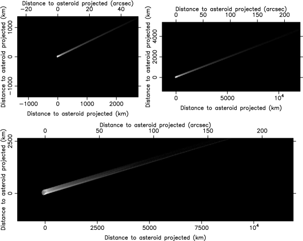
Figure 5: Simulated tail images of Didymos system as would be seen from Earth after DART impact (assumed to occur on 2022 Sept. 26, 23:14 UT), at three observing dates, 2022 Sept 28 (top left), Sept. 30 (top right), and Oct. 2 (bottom), assuming an ejection speed from Dimorphos surface of $v_{ej}$=0.36 $\mathrm{m\;s^{-1}}$, corresponding to four times the escape velocity of Dimorphos. The plate scale is assumed at 0.25 ″px^-1, and the filter used is a $r$-Sloan. The corresponding brightness range are to 16-13, 19-16, and 20-17 $\mathrm{mag\;arcsec^{-2}}$, respectively. The images are all oriented North up, East to the left.

6.2 Aperture photometry

Aperture photometry also provides very important information on the amount of material ejected and the fraction of such mass which is sent to free space, or, depending on the ejecta velocity, is transferred to Didymos or Dimorphos. We have calculated the variation of the predicted magnitude, as a function of time since DART impact, for several ejecta speeds ranging from the escape velocity of Dimorphos ($v_{esc}$=0.09 $\mathrm{m\;s^{-1}}$) to the upper limit set by the collision experiments mentioned above (Koschny & Grün, 2001), $v$=800 $\mathrm{m\;s^{-1}}$. In the low-speed ejecta regime, i.e., speeds from the escape velocity of Dimorphos up to a few times that value, and for the three observing dates shown in Table  3, we computed the $r$-Sloan magnitudes using 1000 km radii ($\sim$18″) apertures. The results are shown in Table  4, together with the unperturbed magnitude that would be attained in the absence of the DART collision. We can see that under low-speed ejecta conditions the ejecta cloud would give a rather easily detectable signal, with about 3 to 1.4 magnitudes below the “clean” system since the time of impact to 5 days later, respectively. In the case of Deep Impact on comet 9P/Tempel 1, the object experienced a sudden increase in brightness of 2.5 magnitudes after the impact (Meech et al., 2005), in line with that found here. We underline that the low-speed ejecta regime would be prevailing if the shaking mechanism (Tancredi et al., 2022) is dominant.

Table 4: Calculated $r$-Sloan magnitudes after DART impact, as a function of date and ejection speed, relative to Dimorphos escape velocity ($v_{esc}$=0.09 $\mathrm{m\;s^{-1}}$), compared to the unperturbed system magnitude.

Date	$v$=$v_{esc}$	$v$=2$v_{esc}$	$v$=4$v_{esc}$	$v$=8$v_{esc}$	Dust-free
(UT)					mag
Sep/28.0/2022	11.66	11.36	11.28	11.23	14.30
Sep/30.0/2022	13.17	12.68	12.42	12.37	14.34
Oct/02.0/2022	13.96	13.22	12.97	12.92	14.39

Table 5: Dust mass delivered to Didymos and Dimorphos as a function of date and ejection speeds.

Date	Mass to	Mass to	Mass to
(UT)	Didymos	Dimorphos	space
$v$=$v_{esc}$
Sep/28.0/2022	7.9$\times$105	1.5$\times$106	2.7$\times$106
Sep/30.0/2022	1.8$\times$106	1.6$\times$106	1.6$\times$106
Oct/02.0/2022	2.4$\times$106	1.7$\times$106	9.0$\times$105
$v$=2$v_{esc}$
Sep/28.0/2022	1.4$\times$106	8.9$\times$103	3.6$\times$106
Sep/30.0/2022	1.7$\times$106	1.7$\times$104	3.3$\times$106
Oct/02.0/2022	1.9$\times$106	2.0$\times$104	3.1$\times$106
$v$=4$v_{esc}$
Sep/28.0/2022	3.7$\times$105	4.6$\times$104	4.6$\times$106
Sep/30.0/2022	4.9$\times$105	4.9$\times$104	4.5$\times$106
Oct/02.0/2022	5.4$\times$105	5.3$\times$104	4.4$\times$106
$v$=8$v_{esc}$
Sep/28.0/2022	1.5$\times$105	1.4$\times$101	4.9$\times$106
Sep/30.0/2022	1.5$\times$105	1.4$\times$101	4.9$\times$106
Oct/02.0/2022	1.5$\times$105	1.4$\times$101	4.9$\times$106

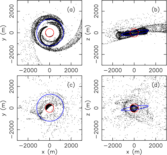
Figure 6: Projection on the $x-y$ and $x-z$ planes of the final position of $r$=1 cm particles on September 28th, 2022. The red circle represents Didymos, and the blue ellipse represents the orbital path of Dimorphos. The upper panels (a) and (b) correspond to ejection velocity $v$=$v_{esc}$, and the lower panels (c) and (d) to $v$=$2v_{esc}$, where $v_{esc}$=0.09 $\mathrm{m\;s^{-1}}$, the escape velocity of Dimorphos.

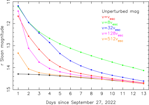
Figure 7: Calculated $r$-Sloan magnitudes as a function of date and ejection velocities, for relatively slow ejection speeds, compared to the unperturbed system magnitude.

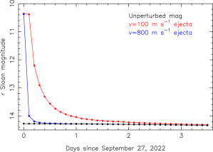
Figure 8: Calculated $r$-Sloan magnitudes as a function of date and ejection velocities, for large ejection speeds, compared to the unperturbed system magnitude.

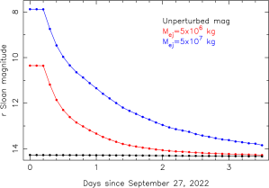
Figure 9: Calculated $r$-Sloan magnitudes as a function of date and total ejected masses of $M_{ej}$=5$\times$10⁶ kg and $M_{ej}$=5$\times$10⁷ kg, for an ejection speed of $v$=512$v_{esc}$=45 $\mathrm{m\;s^{-1}}$, compared to the unperturbed system magnitude.

It is interesting to see that the highest brightness level does not occur at the minimum velocity assumed, $v$=$v_{esc}$, but corresponding to four to eight times that value. This can be explained by the fact that a significant fraction of the mass ejected at such speeds is transferred either to Didymos or Dimorphos. Thus, in Table  5, where we show the fate of the ejected mass, we see that a significant fraction of the ejected mass, up to $\sim$50% in some cases, is sent to one of the binary components when the ejecta is released at speeds of $v$=$v_{esc}$ or $v$=$2v_{esc}$. For larger speeds, we wee that most of the mass is sent to space. In addition, it is also interesting to note that the fate of the mass is different for $v$=$v_{esc}$ and for $v$=$2v_{esc}$. In the former case, a considerable fraction of the mass is, depending on the date, either transferred to Dimorphos (on Sept. 28), or it is shared between Didymos and Dimorphos (Sept. 30, and Oct. 2), while in the latter case, a considerable amount of mass is sent to Didymos while a negligible fraction lands on Dimorphos at all the observing dates. This can be clearly seen in Figure  6 for the first observing date, Sept. 28. In the upper panels (a) and (b), the projections on the $x-y$ and $x-z$ planes of the positions of the particle at the end of integration for $v$=$v_{esc}$, are given. We see that only a few particles stick to Didymos (red circle), while many of them are near the orbital path of Dimorphos, eventually colliding with it. On the contrary, in the lower panels (c) and (d), that correspond to $v$=$2v_{esc}$, we see that many particles got sticked to Didymos, while there are only a few particles near Dimorphos orbit.

At speeds higher than $v$=$8v_{esc}$, the brightness decreases as a function of date at a faster rate, because the particles tend to leave the aperture limits. Figure  7 gives the lightcurves from ejection speeds of $v$=$v_{esc}$ up to $v$=$512v_{esc}$=45 $\mathrm{m\;s^{-1}}$, along with the magnitude of the unperturbed system, using 1000 km aperture radius in all cases. In the most favourable case of $v\sim 8v_{esc}$, the ejecta would give a detectable signal during 13 days or more after impact, but for the higher speed cases the event would be detectable only during 1 day (for $v=512v_{esc}$) to 10 days (for $v=32v_{esc}$) since impact time.

At still higher speeds than those corresponding to Figure  7, the decrease of brightness is dramatic in only a few hours after impact. In Figure  8, lightcurves for ejecta speeds of 100 and 800 $\mathrm{m\;s^{-1}}$, as a function of time, are shown. For $v$=100 $\mathrm{m\;s^{-1}}$, the ejecta would be detectable within one day after impact, while in the least favourable scenario, $v$=800 $\mathrm{m\;s^{-1}}$, the observing window reduces to only $\sim$5 hours at most.

When the total ejected mass is different to that estimated from scaling laws ($M_{ej}\sim$5$\times$10⁶ kg), the observed magnitudes would obviously differ from those shown in the previous graphs. To have an estimate on how much the evolution could be different, in Figure  9 we display the results for an intermediate ejection speed of $v$=$512v_{esc}$=45 $\mathrm{m\;s^{-1}}$, for the nominal mass and for ten times higher that value ($M_{ej}\sim$5$\times$10⁷ kg). In the latter case, a decrease of $\sim$2.5 mag with respect to the nominal mass is foreseen. The flux increment then becomes less and less pronounced as the time passes, the difference between both cases being of only 0.4 magnitudes after 3.5 days. Similar differences are expected for other ejection speeds. Therefore the increase in brightness and its evolution with time will be an useful indicator of the amount of material ejected and the distribution of ejection speeds.

7 Conclusions

Simulations of the dust cloud generated after DART impact on Dimorphos satellite of (65803) Didymos have been performed. The calculations have been made by integrating the equation of motion of a large amount of individual particles ejected from Dimorphos. The total ejected dust mass is calculated on the basis of known scaling laws, being about 5$\times$10⁶ kg. A power-law size distribution function of power index –3.5 and limiting radii of 1 $\mu$m and 1 cm is assumed. Depending on the ejection speed, we give insight on the detectability of such cloud for Earth-based observers. The most favourable ejection scenario for longer term detection would occur when a considerable fraction of the total mass is ejected at speeds of the order of a few times the escape speed of Dimorphos. In such case, aperture photometry measurements would reveal an observed brightness well above the unperturbed system brightness by 1-3 magnitudes for up to 5 days after impact, and a narrow dust tail of length $\lesssim$1′ with 20 $\mathrm{mag\;arcsec^{-2}}$ minimum brightness would be seen in the sky. That would be the case if most of the ejecta is caused by impact-induced seismic waves, producing seismic shaking of the satellite, as the predicted speeds would be below 1 $\mathrm{m\;s^{-1}}$. In the case that the ejecta travels at much larger speeds, of the order of 100 $\mathrm{m\;s^{-1}}$, the brightness increase will be detected only within 2 days after impact time, inducing a fast-decreasing lightcurve from almost 4 to 0.3 magnitudes above the baseline brightness in that time frame. For the highest speeds attainable (following impact experiments) of 800 $\mathrm{m\;s^{-1}}$, the observing window reduces to only $\sim$5 hours after impact at most. This model will serve to constrain the ejecta properties when the corresponding flux measurements become available. The monitoring of the tail and coma brightness in the hours and early days after impact will be relevant for understanding the small particle ejection mechanisms and its contribution to the impact process.

8 Data availability

This work uses simulated data, generated as detailed in the text.

Appendix A Dust tail brightness computation

We start by defining a high-resolution grid of particle radius bins logarithmically distributed in the interval [$r_{min}$,$r_{max}$], where $r_{min}$ and $r_{max}$ are the limits of the particle size distribution function assumed. For each radius bin $[r_{1},r_{2}]$, we computed the trajectories of sampled particles having a mean radius in such bin, $r_{mean}$, whose dynamical behaviour is assumed to be representative of the full $[r_{1},r_{2}]$ range. The number of radius bins was set to 4000. On Dimorphos surface we define a latitude-longitude grid of similar area cells. The particles are ejected radially away from the centre of each cell. The number of latitude$\times$longitude surface elements was set to 20$\times$20. This isotropic ejection pattern can be set to a more realistic ejection pattern once the exact geometry of the impact is known, probably very close to the impact time.

The flux contribution (expressed in magnitudes, $m$) of a spherical particle of radius $a_{p}$ (in metres) falling on a certain pixel of the image on the $(N,M)$ photographic plane is given by the following expression:

$$p_{R}\pi a_{p}^{2}=\frac{2.24\times 10^{22}\pi r_{h}^{2}\Delta^{2}10^{0.4(m_{\odot}-m)}}{G(\alpha)}$$ (6)

where $r_{h}$ is the asteroid heliocentric distance, $\Delta$ is the asteroid geocentric distance (both in au), and $m_{\odot}$ is the apparent solar magnitude in the filter used. All the simulated images in this work refer to $r$-Sloan magnitudes, for which $m_{\odot}$=–26.95 (Ivezić et al., 2001). The particle geometric albedo at zero phase angle is given by $p_{R}$, and $G(\alpha)=10^{-0.4\alpha\phi}$ is the phase angle correction, where $\alpha$ is the phase angle, and $\phi$ is the linear phase coefficient. The contribution to the brightness, $B$, in the mentioned pixel, in units of mag arcsec^-2 would be $B=m+2.5\log_{10}A$, where $A$ is the projected pixel area on the sky in arcsec². To perform the calculations within the computer code, we find most appropriate to work on units of the mean solar disk intensity units in the corresponding wavelength range, $i/i_{\odot}$, where $i_{\odot}=F_{\odot}/\pi$, being $F_{\odot}$ the radiation flux density at the solar surface. Knowing that the solid angle of the Sun disk at a distance of 1 au is $S_{a}$=2.893$\times$10⁶ arcsec², the relation between $i/i_{\odot}$ and $S$ becomes (e.g. Jockers et al., 1992):

$$S=C+m_{\odot}-2.5\log_{10}i/i_{\odot}$$ (7)

where $C=2.5\log_{10}S_{a}=16.153$.

The mass ejected from each surface cell on Dimorphos is given by $M_{cell}=M_{ej}S_{cell}(4\pi R_{sec}^{2})^{-1}$, where $M_{ej}$ is the total dust mass ejected and $S_{cell}$ is the cell surface area. The number of particles ejected from each cell in the bin radius $[r_{1},r_{2}]$ will be given by:

$$N[r_{1},r_{2}]=\frac{3M_{cell}}{4\pi\rho_{p}}\frac{\displaystyle\int_{r_{1}}^{r_{2}}r^{\kappa}dr}{\displaystyle\int_{r_{min}}^{r_{max}}r^{\kappa+3}dr}$$ (8)

where $\kappa$ is the index of the assumed power-law differential size distribution function. Then, if at the end of its trajectory, a particle of radius $r_{mean}$ falls within a certain pixel, the brightness on that pixel would be incremented by the product of $i/i_{0}$ (equation  7) and $N[r_{1},r_{2}]$. The procedure is then carried out for all the 4000 particles ejected from each of the 20$\times$20 aforementioned surface cells on Dimorphos.

References

- Chambers (1999) Chambers J. E., 1999, MNRAS, 304, 793.
- Cheng et al. (2018) Cheng A. F., Rivkin A. S., Michel P., Atchison J., Barnouin O., Benner L., Chabot N. L., et al., 2018, P&SS, 157, 104.
- Dotto et al. (2021) Dotto E., Della Corte V., Amoroso M., Bertini I., Brucato J. R., Capannolo A., Cotugno B., et al., 2021, P&SS, 199, 105185.
- Fang & Margot (2012) Fang J., Margot J.-L., 2012, AJ, 143, 24.
- Finson & Probstein (1968) Finson M. J., Probstein R. F., 1968, ApJ, 154, 327.
- Giblin (1998) Giblin I., 1998, P&SS, 46, 921.
- Grün et al. (1994) Grün E., Gustafson B., Mann I., Baguhl M., Morfill G. E., Staubach P., Taylor A., et al., 1994, A&A, 286, 915
- Housen & Holsapple (2011) Housen K. R., Holsapple K. A., 2011, Icar, 211, 856.
- Ivezić et al. (2001) Ivezić Ž., Tabachnik S., Rafikov R., Lupton R. H., Quinn T., Hammergren M., Eyer L., et al., 2001, AJ, 122, 2749.
- Landgraf (2000) Landgraf M., 2000, JGR, 105, 10303.
- Jewitt et al. (2011) Jewitt D., Weaver H., Mutchler M., Larson S., Agarwal J., 2011, ApJL, 733, L4.
- Jockers et al. (1992) Jockers, K., Bonev, T., Ivanova, V., Rauer, H., 1992, A&A, 260, 455.
- Koschny & Grün (2001) Koschny D., Grün E., 2001, Icarus, 154, 402.
- Meech et al. (2005) Meech K. J., Ageorges N., A’Hearn M. F., Arpigny C., Ates A., Aycock J., Bagnulo S., et al., 2005, Science, 310, 265.
- Michel et al. (2018) Michel P., Kueppers M., Sierks H., Carnelli I., Cheng A. F., Mellab K., Granvik M., et al., 2018, AdSpR, 62, 2261.
- Moreno et al. (2011) Moreno F., Licandro J., Ortiz J. L., Lara L. M., Alí-Lagoa V., Vaduvescu O., Morales N., et al., 2011, ApJ, 738, 130.
- Moreno et al. (2019) Moreno F., Jehin E., Licandro J., Ferrais M., Moulane Y., Pozuelos F. J., Manfroid J., et al., 2019, A&A, 624, L14.
- Moreno et al. (2021) Moreno F., Licandro J., Cabrera-Lavers A., Morate D., Guirado D., 2021, MNRAS, 506, 1733.
- Mukai (1981) Mukai T., 1981, A&A, 99, 1
- Naidu et al. (2020) Naidu S. P., Benner L. A. M., Brozovic M., Nolan M. C., Ostro S. J., Margot J. L., Giorgini J. D., et al., 2020, Icar, 348, 113777.
- Naidu et al. (2021) Naidu, S. P., Chesley S., Farnocchia D. 2021, JPL orbit solution 104 of Dimorphos, IOM 392R-21-008, Jet Propulsion Laboratory
- Pravec et al. (2006) Pravec P., Scheirich P., Kušnirák P., Šarounová L., Mottola S., Hahn G., Brown P., et al., 2006, Icarus, 181, 63.
- Price et al. (2019) Price O., Jones G. H., Morrill J., Owens M., Battams K., Morgan H., Drückmuller M., et al., 2019, Icar, 319, 540.
- Scheirich & Pravec (2009) Scheirich P., Pravec P., 2009, Icar, 200, 531.
- Shevchenko (1997) Shevchenko V. G., 1997, Solar System Research, 31, 219
- Sugita et al. (2005) Sugita S., Ootsubo T., Kadono T., Honda M., Sako S., Miyata T., Sakon I., et al., 2005, Science, 310, 274.
- Tancredi et al. (2022) Tancredi, G. et al., 2022, MNRAS, submitted.
- Yu & Michel (2018) Yu Y., Michel P., 2018, Icarus, 312, 128.