Efficient Verification of Ground States of Frustration-Free Hamiltonians
Abstract
Ground states of local Hamiltonians are of key interest in many-body physics and also in quantum information processing. Efficient verification of these states are crucial to many applications, but very challenging. Here we propose a simple, but powerful recipe for verifying the ground states of general frustration-free Hamiltonians based on local measurements. Moreover, we derive rigorous bounds on the sample complexity by virtue of the quantum detectability lemma (with improvement) and quantum union bound. Notably, the number of samples required does not increase with the system size when the underlying Hamiltonian is local and gapped, which is the case of most interest. As an application, we propose a general approach for verifying Affleck-Kennedy-Lieb-Tasaki (AKLT) states on arbitrary graphs based on local spin measurements, which requires only a constant number of samples for AKLT states defined on various lattices. Our work is of interest not only to many tasks in quantum information processing, but also to the study of many-body physics.
1 Introduction
Multipartite entangled states play key roles in various quantum information processing tasks, including quantum computation, quantum simulation, quantum metrology, and quantum networking. An important class of multipartite states are the ground states of local Hamiltonians, such as Affleck-Kennedy-Lieb-Tasaki (AKLT) states [1, 2] and many tensor-network states [3, 4]. They are of central interest in traditional condensed matter physics and also in the recent study of symmetry-protected topological orders [5, 6, 7, 8]. In addition, such states are particularly appealing to quantum information processing because they can be prepared by cooling down [9] and adiabatic evolution [10, 11, 12, 13, 14] in addition to quantum circuits. Recently, they have found increasing applications in quantum computation and simulation [15, 16, 17, 18, 19, 20, 21]. Notably, AKLT states on various 2D lattices, including the honeycomb lattice, can realize universal measurement-based quantum computation [22, 23, 24, 25, 26, 8].
To achieve success in quantum information processing, it is crucial to guarantee that the underlying multipartite quantum states satisfy desired requirements, irrespective of whether they are prepared by quantum circuits or as ground states of local Hamiltonians. Unfortunately, traditional tomographic methods are notoriously resource consuming. To resolve this problem, many researchers have tried to find more efficient alternatives [27, 28, 29, 30, 31, 20]. Recently, a powerful approach known as quantum state verification (QSV) has attracted increasing attention [32, 33, 34, 35, 36, 37, 38, 39, 40, 41, 42, 43]. Efficient verification protocols based on local measurements have been constructed for many states of practical interest, including bipartite pure states [32, 44, 37, 45, 46, 47, 48], stabilizer states [49, 50, 51, 37, 52, 40, 53, 54, 55], hypergraph states [52], weighted graph states [56], and Dicke states [57, 58]. The efficiency of this approach has been demonstrated in quite a few experiments [59, 60, 61, 62]. Although several works have considered the verification of ground states of local Hamiltonians [33, 35, 36, 21, 63, 38, 14], the sample costs of known protocols are still too prohibitive for large and intermediate quantum systems of practical interest, which consist of more than 100 qubits or qudits, even if the Hamiltonians are frustration free.
In this work, we propose a general recipe for verifying the ground states of frustration-free Hamiltonians based on local measurements, which does not require explicit expressions for the ground states. Each protocol is constructed from a matching cover or edge coloring of a hypergraph encoding the action of the Hamiltonian and is thus very intuitive. Moreover, we derive a rigorous performance guarantee by virtue of the spectral gap of the underlying Hamiltonian and simple graph theoretic quantities, such as the degree and chromatic index (also known as edge chromatic number). For a local Hamiltonian defined on a lattice, to verify the ground state within infidelity and significance level , the sample cost is only , where is the spectral gap of the underlying Hamiltonian. Compared with previous protocols, the scaling behaviors are much better with respect to the system size, spectral gap , and the precision as quantified by the infidelity . Notably, we can verify the ground state with a constant sample cost that is independent of the system size when the spectral gap is bounded from below by a positive constant.
For example, we can verify AKLT states defined on arbitrary graphs, and the resource overhead is upper bounded by a constant that is independent of the system size for most AKLT states of practical interest, including those defined on various 1D and 2D lattices. When and the number of nodes is around 100, our protocols are tens of thousands of times more efficient than previous protocols, and the efficiency advantage becomes more and more significant as the target precision and system size increase. Additional details can be found in the companion paper [64] (see Appendix D). Our recipe is expected to find diverse applications in quantum information processing and many-body physics.
Technically, a frustration-free Hamiltonian is relatively easy to deal with because such a Hamiltonian offers the possibility of parallel verification of multiple local terms simultaneously. High degree of parallel processing is crucial to achieving a high efficiency. Nevertheless, it is still nontrivial to combine the local information as efficiently as possible so as to draw an accurate conclusion about the ground state of the whole Hamiltonian, although the basic idea is quite intuitive. Our main contribution in this work is to construct nearly optimal verification protocols and to derive nearly tight bounds on the sample complexity by fully exploiting the frustration-free property.
To establish our main results on the sample complexity, we first derive a stronger quantum detectability lemma, which improves over previous results [65, 66]. This stronger detectability lemma can be used to derive tighter upper bounds on the operator norm of certain product of projectors tied to the projectors that compose the Hamiltonian; it is also of general interest that is beyond the focus of this paper. In addition, by virtue of a generalization of the quantum union bound [67, 68], we derive a simple, but nearly tight lower bound on the spectral gap of the average of certain test projectors based on the operator norm of a product. Combining these technical tools we derive our main result Theorem 1, which clarifies the spectral gap and sample complexity of our verification protocol. Other main results (including Theorems 2 and 3), once formulated, can be proved by virtue of standard arguments widely used in quantum information theory. Familiarity with the concepts of spherical -designs [69, 70, 71] and spin coherent states [72] would be helpful to understanding the proof of Theorem 3.
The rest of this paper is organized as follows. In Sec. 2 we first review the basic framework of quantum state verification and discuss its generalization to subspace verification. Then we introduce basic concepts on hypergraphs and frustration-free Hamiltonians that are relevant to the current study. In Sec. 3 we prove a stronger detectability lemma and discuss its implications. In Sec. 4 we propose a general approach for verifying the ground states of frustration-free Hamiltonians and determine the sample complexity. In Sec. 5 we illustrate the power of this simple idea by constructing efficient protocols for verifying general AKLT states. Section 6 summarizes this paper.
2 Preliminaries
2.1 Quantum state verification
Consider a device that is supposed to produce the target state within the Hilbert space , but actually produces the states in runs. Our task is to verify whether these states are sufficiently close to the target state on average, where the closeness is usually quantified by the fidelity. To this end, in each run we can perform a random test from a set of accessible tests. Each test is essentially a two-outcome measurement and is determined by the test operator , which satisfies the condition , so that the target state can always pass the test [37, 39, 40].
Suppose the test is chosen with probability ; then the performance of the verification procedure is determined by the verification operator . If is a quantum state that satisfies , then the probability that can pass each test on average satisfies
| (1) |
where is the second largest eigenvalue of , and is the spectral gap from the maximum eigenvalue. To verify the target state within infidelity and significance level (assuming ), the minimum number of tests required reads [37, 39, 40]
| (2) |
which is inversely proportional to the spectral gap . To optimize the performance, we need to maximize the spectral gap over the accessible measurements. The verification operator is homogeneous if it has the following form [39, 40]
| (3) |
where is a real number. Such a verification strategy is also useful for fidelity estimation and is thus particularly appealing.
2.2 Subspace verification
Next, we generalize the idea of QSV to subspace verification, which is crucial to verifying ground states of local Hamiltonians. Previously, the idea of subspace verification was employed only in some special setting [50]. Consider a device that is supposed to produce a quantum state supported in a subspace within the Hilbert space , but may actually produce something different. To this end, in each run we can perform a random test from a set of accessible tests. Each test is determined by a test operator as in QSV. Let be the projector onto the subspace . Then the condition in QSV should now be replaced by , so that every state supported in can always pass each test. Suppose the test is performed with probability ; then the performance of the verification procedure is determined by the verification operator , which is analogous to the counterpart in QSV. The verification operator is homogeneous if it has the following form [cf. Eq. (3)]
| (4) |
where is a real number.
Suppose the quantum state produced has fidelity at most , which means ; then the maximal probability that can pass each test on average reads
| (5) |
where
| (6) |
and is also called the spectral gap. The number of tests required to verify the subspace within infidelity and significance level is still given by Eq. (2), although the meaning of is a bit different now.
2.3 Hypergraphs
A hypergraph is specified by a set of vertices and a set of edges (hyperedges) , where each edge is a nonempty subset of [73, 52]. An edge is a loop if it contains only one vertex. Two distinct vertices of are neighbors or adjacent if they belong to a same edge. The degree of a vertex is the number of its neighbors and is denoted by ; the degree of is the maximum vertex degree and is denoted by . The hypergraph is connected if for each pair of distinct vertices , there exist a positive integer and vertices with and such that are adjacent for .
Two distinct edges of are neighbors or adjacent if their intersection is nonempty. A subset of is a matching of if no two edges in are adjacent. A set of matchings is a matching cover if it covers , which means . It should be noted that, in some literature, a matching cover means a set of matchings that covers the vertex set, which is different from our definition. An edge coloring of is an assignment of colors to its edges such that adjacent edges have different colors. The edge coloring is trivial if no two edges are assigned with the same color. Note that every edge coloring of determines a matching cover. Conversely, every matching cover composed of disjoint matchings determines an edge coloring. The chromatic index (also known as edge chromatic number) of is the minimum number of colors required to color the edges of and is denoted by ; it is also the minimum number of matchings required to cover the edge set .
A (simple) graph is a special hypergraph in which each edge contains two vertices. According to Vizing’s theorem [74, 73], the chromatic index of a graph satisfies
| (7) |
In general, it is computationally very demanding to find an optimal edge coloring, but it is easy to construct a nearly optimal edge coloring with colors [75].
2.4 Frustration-free Hamiltonians
Since we are mainly interested in the ground states, without loss of generality, we can assume that the Hamiltonian is a sum of projectors, which share a common null vector. These projectors can be labeled by the edges (hyperedges) of a hypergraph [73, 52], and can be expressed as
| (8) |
where the projector acts (nontrivially) only on the nodes associated with the vertices contained in .
Given that is frustration free by assumption,
a state is a ground state iff for all , so the ground state energy is 0. The spectral gap of is the smallest nonzero eigenvalue and is denoted by (note the distinction from the spectral gap of a verification operator). The Hamiltonian is -local if each projector acts on at most nodes, in which case each edge of contains at most vertices. Let be the smallest integer such that each projector commutes with all other projectors except for of them.
3 A stronger detectability lemma
The detectability lemma proved in Ref. [65] and improved in Ref. [66] is a powerful tool for understanding the properties of frustration-free Hamiltonians, including the spectral gaps in particular. Here we shall derive a stronger version of the detectability lemma and discuss its implications. This result will be very useful to deriving tighter bounds on the sample cost of our verification protocols for the ground states, which is our original motivation. We believe that it is also of independent interest to many researchers in the quantum information community.
3.1 Improvement of the detectability lemma
The following improvement of the detectability lemma and its corollary Lemma 2 are proved in Sec. 3.2.
Lemma 1.
Let be a set of projectors on a given Hilbert space , , and . Let be any normalized ket in , , and with (assuming ). Then
| (9) |
with and , where is the largest singular value of that is not equal to 1 ( if all singular values of are equal to 1), and
| (10) | |||
| (11) |
Here the last upper bound in Eq. (9) was derived in Ref. [66], while the first three bounds improve over the original result.
To appreciate the implications of Lemma 1, suppose the Hamiltonian in Lemma 1 is frustration free, and is orthogonal to the ground state space. Then is also orthogonal to the ground state space, which means and
| (12) |
Here the last upper bound was derived in Ref. [66]. Our improvement of the detectability lemma presented in Lemma 1 is crucial to deriving the first three upper bounds, which in turn are crucial to deriving Lemma 2 and Theorem 1 below. This improvement can sometimes significantly reduce the upper bound on the number of tests required to verify the ground state of a frustration-free Hamiltonian, as we shall see in Sec. 4.
Lemma 2.
Suppose the Hamiltonian in Lemma 1 is frustration free; let be the projector onto the ground state space of and
| (13) |
Then
| (14) |
3.2 Proofs of Lemmas 1 and 2
Proof of Lemma 1.
To start with, we shall derive an upper bound for . Following Ref. [66], to derive an upper bound for
| (15) |
we can move the projector to the right until it is annihilated by . Only those terms that do not commute with will contribute to the upper bound.
For let
| (16) |
then . By virtue of Lemma 3 below we can deduce that
| (17) |
where is the largest singular value of that is not equal to 1 (note that ). So
| (18) |
where is defined in Eq. (11) and denotes the set of indices of the projectors that do not commute with . As a corollary,
| (19) |
where is the cardinality of .
Lemma 3.
Suppose and are two projectors on and . Then
| (25) |
where is the largest singular value of that is not equal to 1 ( if all singular values of are equal to 1).
Equation (25) holds even if is not normalized.
4 Efficient verification of ground states
4.1 Matching and coloring protocols
Suppose the Hamiltonian in Eq. (8) has a nondegenerate ground state denoted by (the nondegeneracy assumption is included to simplify the description and is not crucial). Let ; then and for all . To verify the ground state, we need to verify that the state is supported in the range of for each , which can be realized by subspace verification. A verification protocol (operator) for an edge is referred to as a bond verification protocol (operator). Since and for each edge only act on a few nodes, it is much easier to construct bond verification protocols than protocols for the ground state. Here we provide a general recipe for constructing verification protocols for the ground state given a bond verification protocol with verification operator for each edge . Note that the operator should satisfy the conditions and . Since is a projector, it follows that the largest eigenvalue of is 1 and its multiplicity is at least the rank of ; all other eigenvalues of belong to the interval . Let
| (27) | ||||||
| (28) |
then is the spectral gap of , and is the minimum spectral gap over all bond verification operators.
In many cases of practical interest, the underlying Hamiltonian has a high symmetry (say the symmetry of a square lattice), and it is possible to construct bond verification operators that are unitarily equivalent to each other. Accordingly, all for are equal, and so are all for , which means and .
Given a matching of , we can construct a test for the ground state by performing the bond verification strategy for each independently. The resulting test operator reads
| (29) |
Note that all for commute with each other, so the order in the product does not matter. In addition, a state satisfies iff for each . So the state can pass the test with certainty iff it belongs to the null space of for each .
Let be a matching cover of that consists of matchings, so that . For each matching , we can construct a test by Eq. (29). Then only the target state can pass each test with certainty. Let be a probability distribution on , then we can construct a matching protocol for by performing the test with probability for . The resulting verification operator reads
| (30) |
which can be abbreviated as when the probability distribution is uniform, that is, for .
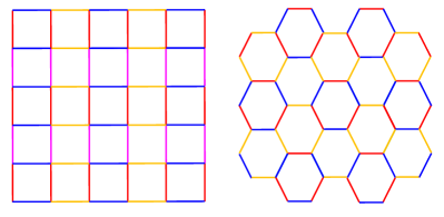
When the matchings in are mutually disjoint, determines an edge coloring of , as illustrated in Fig. 1; the resulting protocol is called an edge coloring protocol or coloring protocol in short. Such a protocol has a very simple graphical description and is thus quite appealing.
4.2 Sample complexity
The efficiency of the matching protocol is guaranteed by Theorem 1 below, which can be proved by virtue of the improved detectability lemma and quantum union bound [67, 68], as shown in Sec. 4.3.
Theorem 1.
Suppose is the frustration-free Hamiltonian in Eq. (8). Let be the verification operator associated with the matching cover of and bond verification operators . Then
| (31) |
where is the minimum spectral gap of , is defined as in Lemma 1, and
| (32) |
The number of tests required to verify the ground state within infidelity and significance level satisfies
| (33) |
The weaker bound in Eq. (31) and that in Eq. (33) can already clarify the sample complexity of the matching protocol. The stronger bounds in the two equations are slightly more complicated and rely on the stronger detectability lemma, that is, Lemma 1. On the other hand, this improvement can sometimes significantly reduce the upper bound on the number of tests (though not the scaling behavior) required to verify the ground state of a frustration-free Hamiltonian. In the verification of the AKLT state on the honeycomb lattice for example, the first lower bound in Eq. (31) is about six times of the second lower bound. So the number of tests in Eq. (33) can be reduced by a factor of six thanks to the stronger bound, which can make a huge difference for practical applications.
It is instructive to analyze the lower bound for the spectral gap in Eq. (31) when , which holds in most cases of practical interest. When , the function can be approximated as
| (34) |
Therefore, the spectral gap can be bounded from below as follows,
| (35) |
which is tighter than the second bound in Eq. (31). Accordingly, the number of tests required to verify the ground state within infidelity and significance level satisfies
| (36) |
If the underlying Hamiltonian is 2-local and each projector acts on two nodes, then is a (simple) graph and , where is the degree of , so Theorem 1 implies that
| (37) |
The cardinality of the matching cover is at least the chromatic index , which satisfies by Vizing’s theorem [74, 73]. If is optimal, that is, , then Eq. (37) yields
| (38) |
Here and do not grow with the system size for most Hamiltonians of practical interest, including those defined on various lattices as illustrated in Fig. 1. If in addition the spectral gap has a universal lower bound, then the spectral gap has a universal lower bound, so the number of tests required to verify the ground state does not grow with the system size. Compared with previous works [33, 35, 36, 21, 63, 38, 14], our approach can achieve much better scaling behaviors with respect to the system size, spectral gap , and infidelity .
Since coloring protocols are special matching protocols, all results on matching protocols presented above also apply to coloring protocols. In addition, we can derive the following result tailored to coloring protocols; see Sec. 4.4 for a proof.
Theorem 2.
Suppose the matching cover in Theorem 1 is actually an edge coloring of and ; then
| (39) |
The inequality is saturated if is the trivial edge coloring with and all bond verification operators are homogeneous and have the same spectral gap.
If is 2-local and each projector acts on two nodes, then , so Theorem 2 means
| (40) |
4.3 Proof of Theorem 1
Proof of Theorem 1.
For let be the test operators associated with the matchings as defined in Eq. (29). Let
| (41) | |||
| (42) |
Then are test projectors for the ground state , and is a verification operator for , although in general they cannot be realized by local measurements.
Next, we prove an auxiliary lemma employed in the proof of Theorem 1.
Lemma 4.
Proof of Lemma 4.
Let
| (48) | |||
| (49) |
then are projectors. First, suppose the matchings in are mutually disjoint, so that corresponds to an edge coloring. If in addition , then
| (50) |
Here the first inequality follows from Lemma 5 below; the second inequality follows from Lemma 2, which implies that
| (51) |
where is defined as in Lemma 1. The last three inequalities in Eq. (50) are due to the following inequalities
| (52) |
and the fact that the function is monotonically increasing in for , which is clear from the definition in Eq. (32).
Meanwhile, we have and , which means . So Eq. (50) implies that
| (53) |
which confirms Eq. (47). Note that the function is monotonically increasing and concave in for .
When , the first inequality in Eq. (50) can be improved by Lemma 5 below, then Eq. (47) follows from a similar reason as presented above.
Next, we turn to the general situation in which the matchings in are not necessarily disjoint. In this case, we can always construct a matching cover composed of mutually disjoint matchings that satisfy for . Let
| (54) |
Then
| (55) |
which implies that
| (56) |
This observation completes the proof of Lemma 4. ∎
Lemma 5.
Suppose are projectors acting on the Hilbert space . Let ; then
| (57) |
If , then
| (58) |
4.4 Proof of Theorem 2
Proof of Theorem 2.
Let be the test operator associated with the matching as defined in Eq. (29). Then
| (59) |
which implies Eq. (39). Here the third equality holds because , , and all matchings in are pairwise disjoint.
If is the trivial edge coloring, then each matching contains only one edge, so that and for . Consequently, the first inequality in Eq. (59) is saturated. If in addition all bond verification operators are homogeneous and have the same spectral gap, then the second inequality in Eq. (59) is also saturated, which means
| (60) | ||||
| (61) |
So the inequality in Eq. (39) is saturated in this case. ∎
5 Efficient verification of AKLT states
To illustrate the power of our general recipe, here we consider AKLT states defined on general graphs without loops; see Appendix D and the companion paper [64] for more details. For any given graph , an AKLT Hamiltonian can be constructed as follows [1, 2, 76, 77]. For each vertex we assign a spin operator with spin value , which corresponds to a Hilbert space of dimension . Let for each edge and ; then . Let be the projector onto the spin- subspace of spins and ; then the AKLT Hamiltonian can be expressed as ; it is frustration free and has a unique ground state [76, 77], which is denoted by .
5.1 Protocols and sample complexity
To verify the AKLT state , we need to construct suitable bond verification protocols. This is a two-body problem for any given bond , so we focus on the two nodes connected by and ignore all other nodes for the moment. Given any real unit vector in dimension 3, let be the spin operator along direction . Then has eigenvalues, namely, . Now a bond test can be constructed as follows: both parties perform the spin measurement along direction , and the test is passed unless they both obtain the maximum eigenvalues or both obtain the minimum eigenvalues.
Let () be the eigenstate of tied to the maximum eigenvalue (minimum eigenvalue ). Define in a similar way and let
| (62) |
Then the bond test projector can be expressed as
| (63) |
which satisfies as expected. The trace of this test projector reads
| (64) |
In addition, , so the tests associated with antipodal points on the unit sphere are identical. As shown in Sec. IV A in the companion paper [64], tests of the form are the optimal choice based on spin measurements.
Let be a probability distribution on the unit sphere; then we can construct a bond verification protocol by performing each test according to . The resulting bond verification operator reads
| (65) |
According to Eq. (64), its trace is given by
| (66) |
which is independent of . Let and be two probability distributions on the unit sphere and with . Then by definition it is straightforward to verify that
| (67) |
If in addition is related to by an orthogonal transformation (rotation or reflection) on the unit sphere, then . The two properties are summarized in the following proposition, which is very helpful to studying the spectral gap of .
Proposition 1.
The spectral gap is concave in and invariant under orthogonal transformations on the unit sphere.
By Proposition 1, the spectral gap is maximized when is the isotropic distribution, which leads to the isotropic protocol; the resulting verification operator is denoted by . By construction is invariant under orthogonal transformations, so it is block diagonal with respect to the spin subspaces associated with total spins , respectively, and it can be expressed as a weighted sum of projectors onto these spin subspaces. Meanwhile, satisfies the conditions and , where and is the projector onto the subspace associated with the maximum total spin . Note that and have ranks and , respectively. In conjunction with Eq. (66) we can now deduce that is homogeneous and has the form
| (68) |
which means . The spectral gap of any other verification operator based on spin measurements satisfies .
Optimal bond verification protocols can also be constructed from discrete distributions based on (spherical) -designs, which are more appealing to practical applications. Given a positive integer , a probability distribution on the unit sphere is a -design if the average of any polynomial of degree at most equals the average over the isotropic distribution [69, 70, 71]. The following theorem offers a general recipe for constructing optimal bond verification protocols, which can be proved by virtue of the theories of -designs [69, 70, 71] and spin coherent states [72], as shown in Sec. 5.2.
Theorem 3.
Let be a probability distribution on the unit sphere and let be the average of and its center inversion. Then the four statements below are equivalent.
-
1.
.
-
2.
.
-
3.
is homogeneous.
-
4.
forms a spherical -design with .
Here is center symmetric by construction, so is a ()-design iff it is a ()-design. Note that -designs for the two-dimensional sphere can be constructed using points [78, 79], so optimal bond verification protocols can be constructed using tests based on spin measurements. For example, the uniform distributions on the vertices of the regular tetrahedron, octahedron, cube, icosahedron, and dodecahedron are -designs with , respectively. A -design can be constructed from certain orbit of the rotational symmetry group of the cube [80, 64]. A 9-design can be constructed from a suitable combination of the icosahedron and dodecahedron [81, 64].
For simplicity we can choose the same distribution for each bond verification protocol (although this is not compulsory). Let be a matching cover of that is composed of matchings and let be a probability distribution on (which can be omitted for the uniform distribution). Then the triple specifies a verification protocol for the AKLT state . Suppose forms a -design with , is an optimal matching cover (or edge coloring) with , and is uniform. By Theorem 1 with , , and , the spectral gap of the resulting verification operator satisfies
| (69) |
given that . So the number of tests required to verify the AKLT state within infidelity and significance level satisfies
| (70) |
which leads to an upper bound that is independent of the system size when is bounded from below by a positive constant and is bounded from above by an integer. Notably, this is the case for various 1D and 2D lattices [1, 2, 82, 83, 84, 85, 86, 87, 8].
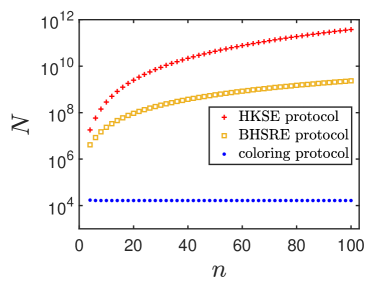
The efficiency of our approach is illustrated in Fig. 2. To verify the AKLT state on the closed chain with 100 nodes within precision , only tests are required. For the honeycomb lattice with 100 nodes, only tests are required. By contrast, all protocols known previously would require tens of thousands of times more tests as explained in Appendix E.
When the degree of is large (compared with ), Theorem 2 may offer better bounds for the spectral gap and the number of tests. Suppose and ; then
| (71) | ||||
| (72) |
given that .
5.2 Proof of Theorem 3
Proof of Theorem 3.
Let
| (73) |
then is a positive operator supported in the range of the projector , which has rank , and we have
| (74) |
In addition,
| (75) |
which implies that
| (76) |
Suppose ; then
| (77) |
This equation implies that has rank and all nonzero eigenvalues are equal given that is a positive operator supported in the range of the projector , which has rank . So is necessarily proportional to . In conjunction with the trace formula derived above we can deduce that
| (78) |
which confirms the implication . The implication is obvious.
Suppose is homogeneous; then it has the form
| (79) |
which means . In addition,
| (80) |
which confirms the implication . So statements 1, 2, 3 are equivalent.
Lemma 6.
Let be a probability distribution on the unit sphere and the bond verification operator based on . Then
| (83) |
and the inequality is saturated iff is a -design with .
6 Summary
We proposed a general recipe for verifying the ground states of frustration-free Hamiltonians based on local measurements. We also provided rigorous bounds on the sample cost required to achieve a given precision by virtue of the spectral gap of the underlying Hamiltonian and simple graph theoretic quantities, as presented in Theorems 1 and 2. The sample complexity achieved by our recipe is optimal with respect to the target precision as quantified by the infidelity and significance level. When the Hamiltonian is local and gapped in the thermodynamic limit, the sample complexity is independent of the system size and is thus optimal with respect to the system size as well. Nevertheless, we believe that the stronger detectability lemma (Lemma 1) we proved can be further improved by a constant factor. Accordingly, the constant in Theorem 1 can be further improved. In any case, our approach can achieve much better scaling behaviors with respect to the system size, spectral gap, and infidelity compared with alternative approaches known before.
To demonstrate the power of this recipe, we constructed concrete protocols for verifying AKLT states defined on arbitrary graphs based on local spin measurements, which are dramatically more efficient than previous protocols. For AKLT states defined on many lattices, including the 1D chain and honeycomb lattice, the sample cost does not increase with the system size. Our work reveals an intimate connection between the quantum verification problem and many-body physics. The protocols we constructed are useful not only to addressing various tasks in quantum information processing, but also to studying many-body physics.
The verification strategy considered in this work can make a meaningful conclusion only if all tests are passed. In practice, it is unrealistic to prepare the perfect target state, and even states with a high fidelity may fail to pass some tests when the total test number is large. In addition, imperfection in the measurement devices may also cause some failures. To construct a robust verification protocol, it is necessary to allow certain failure rate. Fortunately, this extension will only incur a constant overhead [55]. For a typical choice of the allowed failure rate, the overhead is about ten times. So all of our conclusions are still applicable after minor modification even if robustness is taken into account. In addition, by virtue of the recipe proposed in Refs. [39, 40, 55], our protocols can be generalized to the adversarial scenario in which the preparation device cannot be trusted; moreover, the sample overhead is negligible if robustness is not a concern or if homogeneous strategies can be constructed. In general, it is still an open problem to construct robust and efficient verification protocols in the adversarial scenario, which deserves further study.
Our verification protocols can only extract information about the fidelity with the target state. Nevertheless, this key information is very useful in many applications in quantum information processing. One of the main goals in the active research area of quantum characterization, verification, and validation (QCVV) [27, 28, 29, 30, 31] is to extract such key information as efficiently as possible given the limited resources available, which is the best we can do. Even if this key information is not enough in certain situations, it is still valuable as a first-step diagnosis before taking more sophisticated methods. To extract more information necessarily means more resource overhead. Actually, other characterization methods, such as quantum tomography, usually require substantially (often exponentially) more resources.
References
- [1] I. Affleck, T. Kennedy, E. H. Lieb, and H. Tasaki. “Rigorous results on valence-bond ground states in antiferromagnets”. Phys. Rev. Lett. 59, 799–802 (1987).
- [2] I. Affleck, T. Kennedy, E. H. Lieb, and H. Tasaki. “Valence bond ground states in isotropic quantum antiferromagnets”. Commun. Math. Phys. 115, 477–528 (1988).
- [3] D. Pérez-García, F. Verstraete, M. M. Wolf, and J. I. Cirac. “PEPS as unique ground states of local Hamiltonians”. Quantum Info. Comput. 8, 650–663 (2008).
- [4] J. I. Cirac, D. Pérez-García, N. Schuch, and F. Verstraete. “Matrix product states and projected entangled pair states: Concepts, symmetries, theorems”. Rev. Mod. Phys. 93, 045003 (2021).
- [5] X. Chen, Z.-C. Gu, Z.-X. Liu, and X.-G. Wen. “Symmetry-protected topological orders in interacting Bosonic systems”. Science 338, 1604–1606 (2012).
- [6] T. Senthil. “Symmetry-protected topological phases of quantum matter”. Annu. Rev. Condens. Matter Phys. 6, 299–324 (2015).
- [7] C.-K. Chiu, J. C. Y. Teo, A. P. Schnyder, and S. Ryu. “Classification of topological quantum matter with symmetries”. Rev. Mod. Phys. 88, 035005 (2016).
- [8] T.-C. Wei, R. Raussendorf, and I. Affleck. “Some aspects of Affleck–Kennedy–Lieb–Tasaki models: Tensor network, physical properties, spectral gap, deformation, and quantum computation”. In Entanglement in Spin Chains, edited by A. Bayat, S. Bose, and H. Johannesson, pages 89–125. Springer. (2022).
- [9] F. Verstraete, M. M. Wolf, and J. I. Cirac. “Quantum computation and quantum-state engineering driven by dissipation”. Nat. Phys. 5, 633–636 (2009).
- [10] E. Farhi, J. Goldstone, S. Gutmann, and M. Sipser. “Quantum computation by adiabatic evolution” (2000). arXiv:quant-ph/0001106.
- [11] E. Farhi, J. Goldstone, S. Gutmann, J. Lapan, A. Lundgren, and D. Preda. “A quantum adiabatic evolution algorithm applied to random instances of an NP-complete problem”. Science 292, 472–475 (2001).
- [12] T. Albash and D. A. Lidar. “Adiabatic quantum computation”. Rev. Mod. Phys. 90, 015002 (2018).
- [13] Y. Ge, A. Molnár, and J. I. Cirac. “Rapid adiabatic preparation of injective projected entangled pair states and Gibbs states”. Phys. Rev. Lett. 116, 080503 (2016).
- [14] E. Cruz, F. Baccari, J. Tura, N. Schuch, and J. I. Cirac. “Preparation and verification of tensor network states”. Phys. Rev. Research 4, 023161 (2022).
- [15] D. T. Stephen, D.-S. Wang, A. Prakash, T.-C. Wei, and R. Raussendorf. “Computational power of symmetry-protected topological phases”. Phys. Rev. Lett. 119, 010504 (2017).
- [16] R. Raussendorf, C. Okay, D.-S. Wang, D. T. Stephen, and H. P. Nautrup. “Computationally universal phase of quantum matter”. Phys. Rev. Lett. 122, 090501 (2019).
- [17] D. T. Stephen, H. P. Nautrup, J. Bermejo-Vega, J. Eisert, and R. Raussendorf. “Subsystem symmetries, quantum cellular automata, and computational phases of quantum matter”. Quantum 3, 142 (2019).
- [18] A. K. Daniel, R. N. Alexander, and A. Miyake. “Computational universality of symmetry-protected topologically ordered cluster phases on 2D Archimedean lattices”. Quantum 4, 228 (2020).
- [19] M. Goihl, N. Walk, J. Eisert, and N. Tarantino. “Harnessing symmetry-protected topological order for quantum memories”. Phys. Rev. Research 2, 013120 (2020).
- [20] D. Hangleiter and J. Eisert. “Computational advantage of quantum random sampling”. Rev. Mod. Phys. 95, 035001 (2023).
- [21] J. Bermejo-Vega, D. Hangleiter, M. Schwarz, R. Raussendorf, and J. Eisert. “Architectures for quantum simulation showing a quantum speedup”. Phys. Rev. X 8, 021010 (2018).
- [22] R. Kaltenbaek, J. Lavoie, B. Zeng, S. D. Bartlett, and K. J. Resch. “Optical one-way quantum computing with a simulated valence-bond solid”. Nat. Phys. 6, 850 (2010).
- [23] T.-C. Wei, I. Affleck, and R. Raussendorf. “Affleck-Kennedy-Lieb-Tasaki state on a honeycomb lattice is a universal quantum computational resource”. Phys. Rev. Lett. 106, 070501 (2011).
- [24] A. Miyake. “Quantum computational capability of a 2D valence bond solid phase”. Ann. Phys. 326, 1656–1671 (2011).
- [25] T.-C. Wei, I. Affleck, and R. Raussendorf. “Two-dimensional Affleck-Kennedy-Lieb-Tasaki state on the honeycomb lattice is a universal resource for quantum computation”. Phys. Rev. A 86, 032328 (2012).
- [26] T.-C. Wei. “Quantum spin models for measurement-based quantum computation”. Adv. Phys.: X 3, 1461026 (2018).
- [27] J. Eisert, D. Hangleiter, N. Walk, I. Roth, D. Markham, R. Parekh, U. Chabaud, and E. Kashefi. “Quantum certification and benchmarking”. Nat. Rev. Phys. 2, 382–390 (2020).
- [28] J. Carrasco, A. Elben, C. Kokail, B. Kraus, and P. Zoller. “Theoretical and experimental perspectives of quantum verification”. PRX Quantum 2, 010102 (2021).
- [29] M. Kliesch and I. Roth. “Theory of quantum system certification”. PRX Quantum 2, 010201 (2021).
- [30] X.-D. Yu, J. Shang, and O. Gühne. “Statistical methods for quantum state verification and fidelity estimation”. Adv. Quantum Technol. 5, 2100126 (2022).
- [31] J. Morris, V. Saggio, A. Gočanin, and B. Dakić. “Quantum verification and estimation with few copies”. Adv. Quantum Technol. 5, 2100118 (2022).
- [32] M. Hayashi, K. Matsumoto, and Y. Tsuda. “A study of LOCC-detection of a maximally entangled state using hypothesis testing”. J. Phys. A: Math. Gen. 39, 14427 (2006).
- [33] M. Cramer, M. B. Plenio, S. T. Flammia, R. Somma, D. Gross, S. D. Bartlett, O. Landon-Cardinal, D. Poulin, and Y.-K. Liu. “Efficient quantum state tomography”. Nat. Commun. 1, 149 (2010).
- [34] L. Aolita, C. Gogolin, M. Kliesch, and J. Eisert. “Reliable quantum certification of photonic state preparations”. Nat. Commun. 6, 8498 (2015).
- [35] B. P. Lanyon, C. Maier, M. Holzäpfel, T. Baumgratz, C. Hempel, P. Jurcevic, I. Dhand, A. S. Buyskikh, A. J. Daley, M. Cramer, M. B. Plenio, R. Blatt, and C. F. Roos. “Efficient tomography of a quantum many-body system”. Nat. Phys. 13, 1158–1162 (2017).
- [36] D. Hangleiter, M. Kliesch, M. Schwarz, and J. Eisert. “Direct certification of a class of quantum simulations”. Quantum Sci. Technol. 2, 015004 (2017).
- [37] S. Pallister, N. Linden, and A. Montanaro. “Optimal verification of entangled states with local measurements”. Phys. Rev. Lett. 120, 170502 (2018).
- [38] Y. Takeuchi and T. Morimae. “Verification of many-qubit states”. Phys. Rev. X 8, 021060 (2018).
- [39] H. Zhu and M. Hayashi. “Efficient verification of pure quantum states in the adversarial scenario”. Phys. Rev. Lett. 123, 260504 (2019).
- [40] H. Zhu and M. Hayashi. “General framework for verifying pure quantum states in the adversarial scenario”. Phys. Rev. A 100, 062335 (2019).
- [41] Y.-D. Wu, G. Bai, G. Chiribella, and N. Liu. “Efficient verification of continuous-variable quantum states and devices without assuming identical and independent operations”. Phys. Rev. Lett. 126, 240503 (2021).
- [42] Y.-C. Liu, J. Shang, R. Han, and X. Zhang. “Universally optimal verification of entangled states with nondemolition measurements”. Phys. Rev. Lett. 126, 090504 (2021).
- [43] A. Gočanin, I. Šupić, and B. Dakić. “Sample-efficient device-independent quantum state verification and certification”. PRX Quantum 3, 010317 (2022).
- [44] M. Hayashi. “Group theoretical study of LOCC-detection of maximally entangled states using hypothesis testing”. New J. Phys. 11, 043028 (2009).
- [45] H. Zhu and M. Hayashi. “Optimal verification and fidelity estimation of maximally entangled states”. Phys. Rev. A 99, 052346 (2019).
- [46] Z. Li, Y.-G. Han, and H. Zhu. “Efficient verification of bipartite pure states”. Phys. Rev. A 100, 032316 (2019).
- [47] K. Wang and M. Hayashi. “Optimal verification of two-qubit pure states”. Phys. Rev. A 100, 032315 (2019).
- [48] X.-D. Yu, J. Shang, and O. Gühne. “Optimal verification of general bipartite pure states”. npj Quantum Inf. 5, 112 (2019).
- [49] M. Hayashi and T. Morimae. “Verifiable measurement-only blind quantum computing with stabilizer testing”. Phys. Rev. Lett. 115, 220502 (2015).
- [50] K. Fujii and M. Hayashi. “Verifiable fault tolerance in measurement-based quantum computation”. Phys. Rev. A 96, 030301(R) (2017).
- [51] M. Hayashi and M. Hajdušek. “Self-guaranteed measurement-based quantum computation”. Phys. Rev. A 97, 052308 (2018).
- [52] H. Zhu and M. Hayashi. “Efficient verification of hypergraph states”. Phys. Rev. Appl. 12, 054047 (2019).
- [53] Z. Li, Y.-G. Han, and H. Zhu. “Optimal verification of Greenberger-Horne-Zeilinger states”. Phys. Rev. Appl. 13, 054002 (2020).
- [54] D. Markham and A. Krause. “A simple protocol for certifying graph states and applications in quantum networks”. Cryptography 4, 3 (2020).
- [55] Z. Li, H. Zhu, and M. Hayashi. “Robust and efficient verification of graph states in blind measurement-based quantum computation”. npj Quantum Inf. 9, 115 (2023).
- [56] M. Hayashi and Y. Takeuchi. “Verifying commuting quantum computations via fidelity estimation of weighted graph states”. New J. Phys. 21, 093060 (2019).
- [57] Y.-C. Liu, X.-D. Yu, J. Shang, H. Zhu, and X. Zhang. “Efficient verification of Dicke states”. Phys. Rev. Appl. 12, 044020 (2019).
- [58] Z. Li, Y.-G. Han, H.-F. Sun, J. Shang, and H. Zhu. “Verification of phased Dicke states”. Phys. Rev. A 103, 022601 (2021).
- [59] W.-H. Zhang, C. Zhang, Z. Chen, X.-X. Peng, X.-Y. Xu, P. Yin, S. Yu, X.-J. Ye, Y.-J. Han, J.-S. Xu, G. Chen, C.-F. Li, and G.-C. Guo. “Experimental optimal verification of entangled states using local measurements”. Phys. Rev. Lett. 125, 030506 (2020).
- [60] W.-H. Zhang, X. Liu, P. Yin, X.-X. Peng, G.-C. Li, X.-Y. Xu, S. Yu, Z.-B. Hou, Y.-J. Han, J.-S. Xu, Z.-Q. Zhou, G. Chen, C.-F. Li, and G.-C. Guo. “Classical communication enhanced quantum state verification”. npj Quantum Inf. 6, 103 (2020).
- [61] L. Lu, L. Xia, Z. Chen, L. Chen, T. Yu, T. Tao, W. Ma, Y. Pan, X. Cai, Y. Lu, S. Zhu, and X.-S. Ma. “Three-dimensional entanglement on a silicon chip”. npj Quantum Inf. 6, 30 (2020).
- [62] X. Jiang, K. Wang, K. Qian, Z. Chen, Z. Chen, L. Lu, L. Xia, F. Song, S. Zhu, and X. Ma. “Towards the standardization of quantum state verification using optimal strategies”. npj Quantum Inf. 6, 90 (2020).
- [63] M. Gluza, M. Kliesch, J. Eisert, and L. Aolita. “Fidelity witnesses for fermionic quantum simulations”. Phys. Rev. Lett. 120, 190501 (2018).
- [64] T. Chen, Y. Li, and H. Zhu. “Efficient verification of Affleck-Kennedy-Lieb-Tasaki states”. Phys. Rev. A 107, 022616 (2023).
- [65] D. Aharonov, I. Arad, Z. Landau, and U. Vazirani. “The detectability lemma and quantum gap amplification”. In Proceedings of the Forty-First Annual ACM Symposium on Theory of Computing. Page 417–426. STOC’09, New York, NY, USA (2009).
- [66] A. Anshu, I. Arad, and T. Vidick. “Simple proof of the detectability lemma and spectral gap amplification”. Phys. Rev. B 93, 205142 (2016).
- [67] J. Gao. “Quantum union bounds for sequential projective measurements”. Phys. Rev. A 92, 052331 (2015).
- [68] R. O’Donnell and R. Venkateswaran. “The quantum union bound made easy”. In Symposium on Simplicity in Algorithms (SOSA). Pages 314–320. SIAM (2022).
- [69] P. Delsarte, J. M. Goethals, and J. J. Seidel. “Spherical codes and designs”. Geom. Dedicata 6, 363–388 (1977).
- [70] J. J. Seidel. “Definitions for spherical designs”. J. Stat. Plan. Inference 95, 307 (2001).
- [71] E. Bannai and E. Bannai. “A survey on spherical designs and algebraic combinatorics on spheres”. Eur. J. Combinator. 30, 1392–1425 (2009).
- [72] W.-M. Zhang, D. H. Feng, and R. Gilmore. “Coherent states: Theory and some applications”. Rev. Mod. Phys. 62, 867–927 (1990).
- [73] V. I. Voloshin. “Introduction to graph and hypergraph theory”. Nova Science Publishers Inc. New York (2009). URL: https://lccn.loc.gov/2008047206.
- [74] V. G. Vizing. “On an estimate of the chromatic class of a p-graph (Russian)”. Diskret. Analiz 3, 25–30 (1964). URL: https://mathscinet.ams.org/mathscinet/relay-station?mr=0180505.
- [75] J. Misra and D. Gries. “A constructive proof of Vizing’s theorem”. Inf. Process. Lett. 41, 131–133 (1992).
- [76] A. N. Kirillov and V. E. Korepin. “The valence bond solid in quasicrystals” (2009). arXiv:0909.2211.
- [77] V. E. Korepin and Y. Xu. “Entanglement in valence-bond-solid states”. I. J. Mod. Phys. B 24, 1361–1440 (2010).
- [78] A. Bondarenko, D. Radchenko, and M. Viazovska. “Optimal asymptotic bounds for spherical designs”. Ann. Math. 178, 443 (2013).
- [79] R. S. Womersley. “Efficient spherical designs with good geometric properties” (2017). arXiv:1709.01624.
- [80] H. Zhu, R. Kueng, M. Grassl, and D. Gross. “The Clifford group fails gracefully to be a unitary 4-design” (2016). arXiv:1609.08172.
- [81] D. Hughes and S. Waldron. “Spherical half-designs of high order”. Involve 13, 193 (2020).
- [82] A. Garcia-Saez, V. Murg, and T.-C. Wei. “Spectral gaps of Affleck-Kennedy-Lieb-Tasaki Hamiltonians using tensor network methods”. Phys. Rev. B 88, 245118 (2013).
- [83] H. Abdul-Rahman, M. Lemm, A. Lucia, B. Nachtergaele, and A. Young. “A class of two-dimensional AKLT models with a gap”. In Analytic Trends in Mathematical Physics, edited by H. Abdul-Rahman, R. Sims, and A. Young, volume 741 of Contemporary Mathematics, pages 1–21. American Mathematical Society. (2020).
- [84] N. Pomata and T.-C. Wei. “AKLT models on decorated square lattices are gapped”. Phys. Rev. B 100, 094429 (2019).
- [85] N. Pomata and T.-C. Wei. “Demonstrating the Affleck-Kennedy-Lieb-Tasaki Spectral Gap on 2D Degree-3 Lattices”. Phys. Rev. Lett. 124, 177203 (2020).
- [86] M. Lemm, A. W. Sandvik, and L. Wang. “Existence of a spectral gap in the Affleck-Kennedy-Lieb-Tasaki model on the hexagonal lattice”. Phys. Rev. Lett. 124, 177204 (2020).
- [87] W. Guo, N. Pomata, and T.-C. Wei. “Nonzero spectral gap in several uniformly spin-2 and hybrid spin-1 and spin-2 AKLT models”. Phys. Rev. Research 3, 013255 (2021).
Appendix
In this appendix we first prove three auxiliary lemmas employed in the main text, namely Lemmas 3, 5, and 6. Then we briefly discuss the connections with and distinctions from the companion paper [64]. Finally, we compare our verification protocols with previous protocols known in the literature.
Appendix A Proof of Lemma 3
Proof of Lemma 3.
When has dimension 0 or 1, the inequality in Eq. (25) is trivial. In addition, it is easy to verify this inequality when one of the following four conditions holds,
-
1.
or ;
-
2.
or ;
-
3.
;
-
4.
.
So we can exclude these cases in the following discussion. Furthermore, we can assume that is a normalized ket without loss of generality.
Suppose has dimension 2, which is the simplest nontrivial case. In view of the above analysis, we can assume that and are distinct rank-1 projectors that are not orthogonal to each other. Then and correspond to two distinct pure states, denoted by and hence forth. Let be the (normalized) ket that is orthogonal to . Let be the Bloch vectors of , respectively. Let be the angle between and and let be the angle between and , where and , so that . Then we have
| (A1) | |||
| (A2) | |||
| (A3) |
According to the definitions of the vectors and angles introduced above it is easy to verify that
| (A4) |
which implies that
| (A5) |
Therefore,
| (A6) |
which confirms the inequality in Eq. (25).
Now we are ready to consider the most general situation. Denote by and the ranks of and , respectively, and let . Then and have spectral decompositions
| (A7) |
which satisfy
| (A8) |
for and . Without loss of generality, we can assume that if .
Given , let be the subspace spanned by and and let
| (A9) |
Then the subspaces are mutually orthogonal. For , let be the orthogonal projector onto and let
| (A10) |
Then , where for are introduced in Eq. (A8), while (note that ).
Appendix B Proof of Lemma 5
Proof of Lemma 5.
Equation (58) is a simple corollary of Lemma 1 in Ref. [58], so it remains to prove Eq. (57). Let be any normalized ket, and
| (B1) | ||||
| (B2) |
According to Theorem 1.3 in Ref. [68], which is a generalization of the quantum union bound [67], we have
| (B3) |
which implies that
| (B4) |
Now choose as an eigenvector of associated with the largest eigenvalue, that is, . Then the above equation implies that
| (B5) |
which in turn implies Eq. (57). ∎
Appendix C Proof of Lemma 6
Proof of Lemma 6.
As in the proof of Theorem 3, let
| (C1) |
where is defined in Eq. (63). The inequality in Eq. (83) follows from the equality and the fact that is a positive operator supported in the range of the projector , which has rank .
Now, by virtue of Lemma 7 below we can deduce that
| (C2) |
where
| (C3) |
is the th frame potential of the distribution . Note that irrespective of the distribution . When is an even positive integer, the frame potential satisfies the inequality [70, 71]
| (C4) |
which is saturated if forms a spherical -design. Therefore,
| (C5) |
which reproduces the inequality in Eq. (83). Here the second equality follows from the identity below,
| (C6) |
In the rest of this appendix we prove an auxiliary lemma employed in the proof of Lemma 6.
Lemma 7.
With Lemma 7 it is easy to compute the trace since
| (C9) |
Proof of Lemma 7.
By definitions in Eqs. (62) and (63), the kets for any unit vector in dimension 3 belong to the support of , so commutes with and . In addition,
| (C10) |
Similar conclusions also hold if is replaced by .
According to the theory of spin (or atomic) coherent states (see Sec. III D in Ref. [72]), we have
| (C11) | ||||
which implies that
| (C12) | ||||
Appendix D Connections with and distinctions from the companion paper [64]
In this paper, we proposed a general recipe for verifying the ground states of frustration-free Hamiltonians based on local measurements and provided rigorous bounds on the sample cost required to achieve a given precision as formulated in Theorems 1 and 2. To illustrate the power of this general recipe, we constructed efficient protocols for verifying AKLT states based on local spin measurements.
In the companion paper [64], we discussed in more details the verification of AKLT states following the general recipe proposed here and rigorous bounds on the sample cost as presented in Theorems 1 and 2. To be specific, we proved that the tests of the form in Eq. (63) are optimal among tests based on local spin measurements. In addition, the main properties of these tests and corresponding bond verification operators can actually be understood from the perspective of one spin with a suitable spin value instead of two spins, which is very helpful to technical analysis and numerical calculation. Notably, Theorem 3 in Ref. [64], which is the counterpart of Theorem 3 in this paper, is formulated in this perspective. Based on this observation we constructed many concrete bond verification protocols based on platonic solids and other special distributions on the unit sphere, which are optimal or nearly optimal. Then we discussed the optimization of the spectral gaps based on the optimization of matching covers and test probabilities. Furthermore, we constructed a number of concrete verification protocols for AKLT states on open and closed chains and compared their efficiencies based on theoretical analysis and numerical calculation. Finally, we considered AKLT states on arbitrary graphs up to five vertices.
Appendix E Comparison with previous works
In this section we compare our verification protocols for the ground states of frustration-free local Hamiltonians with previous works [38, 33, 35, 36, 21, 14, 63]. It should be noted that the protocols proposed in Refs. [38, 33, 35, 21, 63] are also applicable to certain local Hamiltonians that are not frustration free. The property of being frustration-free is crucial to attaining the high efficiency achieved in this work.
According to the following analysis, previous protocols require at least tests to verify an -qubit target state within infidelity and significance level , where is the spectral gap of the underlying Hamiltonian. In sharp contrast, our protocols require only tests, which is substantially more efficient than previous protocols. Notably, only our protocols can verify the target state with a sample cost that is independent of the system size when the Hamiltonian is gapped in the thermodynamic limit). Moreover, for large and intermediate quantum systems of practical interest (which are beyond classical simulation and are required to demonstrate quantum advantage), only our protocols can achieve the verification task with reasonable sample cost acceptable in experiments or practical applications. When and is around 100 for example, other protocols would require tens of thousands of times more samples to achieve the same precision.
E.1 Comparison with Ref. [38]
In Ref. [38], Takeuchi and Morimae (TM) introduced a protocol for verifying the ground states of local Hamiltonians. To verify an -qubit target state within infidelity and significance level , the number of tests required is given by with
| (E1) |
where , and is the spectral gap of the underlying Hamiltonian . This number is approximately proportional to the fourth power of the inverse spectral gap. The scaling behaviors with and are not clear because the choices of these parameters in Ref. [38] are coupled with the number of qubits. In any case, the number of required tests is astronomical for any verification task of practical interest. When for example, this number is at least , which is billions of times more than what is required in our protocols and is too prohibitive for practical applications.
Incidentally, the TM protocol can be applied to the adversarial scenario in which the preparation device is not trusted. By virtue of the recipe proposed in Refs. [39, 40], our protocols can also be generalized to the adversarial scenario with negligible overhead in the sample cost. In this scenario, our protocols are still dramatically more efficient than the TM protocol.
E.2 Comparison with Refs. [33, 35, 36, 21, 14]
In Ref. [33], Cramer et al. introduced an approach for verifying quantum states that can be approximated by matrix product states (MPS). It is much more efficient than quantum state tomography, but the paper did not give very specific sample cost (see the followup Ref. [35] for a bit more detail). In addition, this approach only applies to one-dimensional systems, which is a bit restricted.
In Ref. [36], Hangleiter, Kliesch, Schwarz, and Eisert (HKSE) extended the approach introduced in Ref. [33] and proposed a general protocol for verifying the ground states of local Hamiltonians, assuming that each local projector can be measured directly. To verify the target state within infidelity and significance level , the number of tests required is given by
| (E2) |
where is the number of edges of the graph encoding the action of the Hamiltonian, that is, the number of local projectors. Here the approximation is applicable when and , which hold for most cases of practical interest. If the Hamiltonian is 2-local and is defined on a lattice with nodes and coordination number , then , so the above equation reduces to
| (E3) |
This number is (approximately) proportional to , , and . The sample complexity is much better than the TM protocol [38] discussed above. However, this number is still too prohibitive for large and intermediate quantum systems of practical interest, which consist of more than 100 qubits or qudits.
In Ref. [21], Bermejo-Vega, Hangleiter, Schwarz, Raussendorf, and Eisert (BHSRE) improved the HKSE protocol and reduced the sample cost to [see Eq. (E10) in the paper]
| (E4) |
where depend on certain decomposition of the underlying Hamiltonian and satisfy the conditions and . Here the scaling behavior in is better than the HKSE protocol, but the scaling behaviors in and remain the same.
Following the idea of the HKSE protocol, Ref. [14] introduced a protocol for verifying a family of tensor network states. The sample cost is proportional to , which is comparable to the BHSRE protocol. However, the proof in Ref. [14] relies on the Gaussian approximation, which is not very rigorous. Notably, Eq. (E2) in Ref. [14] is applicable only under suitable restrictions on the parameters, which were not clarified. Additional analysis is required to derive a rigorous bound on the sample cost.
For example, consider the AKLT state on the closed chain with nodes, in which case and [82, 8]. Suppose we want to verify the target AKLT state within infidelity and significance level . We can apply the optimal coloring protocol, and each bond verification protocol can be constructed from a 4-design [cf. Theorem 3]. According to Theorem 1 with , , , and , the spectral gap of the verification operator is bounded from below by 0.0278, and the number of tests required by our protocol is at most . By contrast, according to Eq. (E2) with , the number of tests required by the HKSE protocol is about , which is 22 million times more than our protocol. According to the lower bound in Eq. (E4) with , the number of tests required by the BHSRE protocol is at least (assuming that BHSRE protocol can be generalized to qudit systems; originally, BHSRE mainly focused on qubit systems), which is 140 thousand times more than our protocol.
Next, consider the AKLT state on the honeycomb lattice with the same number of nodes, in which case and [82, 8]. Now we can apply the optimal coloring protocol as illustrated in Fig. 1 in the main text, and each bond verification protocol can be constructed from a 6-design [cf. Theorem 3]. According to Theorem 1 with , , , , and , the spectral gap of the verification operator is bounded from below by , and the number of tests required by our protocol is at most . By contrast, according to Eq. (E2) with , the number of tests required by the HKSE protocol is about , which is 20 million times more than our protocol. According to the lower bound in Eq. (E4) with , the number of tests required by the BHSRE protocol is at least , which is 37 thousand times more than our protocol. The advantage of our verification protocol is more dramatic as the system size and target precision increase.
In addition, our protocol only uses local projective measurements. If the projectors that compose the Hamiltonian can be measured directly as required in the HKSE protocol, then the bond spectral gap in Theorem 1 can attain the maximum value 1 instead of () for the 1D chain (honeycomb lattice), and the number of tests required by our protocol can be reduced by a factor of () for the 1D chain (honeycomb lattice).
E.3 Comparison with Ref. [63]
In Ref. [63], Gluza, Kliesch, Eisert, and Aolita (GKEA) introduced a protocol for verifying fermionic Gaussian states. The focus and scope of applications are very different from the current work. To verify an -mode fermionic Gaussian state within infidelity and significance level , the sample complexity is about
| (E5) |
When the fermionic Gaussian state is the unique ground state of a gapped local Hamiltonian, the sample complexity can be reduced to
| (E6) |
However, here the constant and scaling behavior with respect to the spectral gap were not clarified in Ref. [63].