Abstract

The loss of magnetic pressure accompanying the decay of the magnetic field in a magnetar may trigger exothermic electron captures by nuclei in the shallow layers of the stellar crust. Very accurate analytical formulas are obtained for the threshold density and pressure, as well as for the maximum amount of heat that can be possibly released, taking into account the Landau–Rabi quantization of electron motion. These formulas are valid for arbitrary magnetic field strengths, from the weakly quantizing regime to the most extreme situation in which electrons are all confined to the lowest level. Numerical results are also presented based on experimental nuclear data supplemented with predictions from the Brussels-Montreal model HFB-24. This same nuclear model has been already employed to calculate the equation of state in all regions of magnetars.

1 1 0 Academic Editor: Firstname Lastname 13 May 2022 8 June 2022 https://doi.org/ Onset of Electron Captures and Shallow Heating in Magnetars Onset of Electron Captures and Shallow Heating in Magnetars Nicolas Chamel ^1,* and Anthea Francesca Fantina ^2,1 Nicolas Chamel and Anthea Francesca Fantina Chamel, N.; Fantina, A.F. Correspondence: nicolas.chamel@ulb.be

1 Introduction

Soft gamma-ray repeaters and anomalous X-ray pulsars are two facets of a very active subclass of neutron stars, called magnetars, exhibiting outbursts and less frequently giant flares that release huge amounts of energy up to $\sim$$10^{46}$ erg within a second (see e.g., Esposito et al. (2021) for a recent review). These phenomena are thought to be powered by internal magnetic fields exceeding $10^{14}$–$10^{15}$ G Duncan and Thompson (1992). At the date of this writing, 24 such objects have been discovered and six more candidates remain to be confirmed according to the McGill Online Magnetar Catalog Olausen and Kaspi (2014). Their persistent X-ray luminosity $\sim$$10^{33}$–$10^{35}$ erg/s, which is well in excess of their rotational energy and which implies a higher surface temperature than in weakly magnetized neutron stars of the same age Viganò et al. (2013), provides further evidence for extreme magnetic fields Beloborodov and Li (2016). It is widely thought that heat is generated by the deformations of the crust beyond the elastic limit due to magnetic stresses (see, e.g., De Grandis et al. (2020)). This mechanism is most effective in the inner region of the crust, where crystallization first occurs Fantina et al. (2020); Carreau et al. (2020). However, it has been demonstrated that heat sources should be located in the shallow region of the crust to avoid excessive neutrino losses Kaminker et al. (2006, 2009). Alternatively, the magnetic energy in the outer crust may be dissipated into heat through electron captures by nuclei triggered by the magnetic field evolution Cooper and Kaplan (2010). This mechanism is analogous to crustal heating in accreting neutron stars Haensel and Zdunik (1990), the matter compression being induced here by the loss of magnetic support rather than accretion from a stellar companion.

We have recently estimated the maximum amount of heat that could be possibly released by electron captures and the location of the heat sources taking into account Landau–Rabi quantization of electron motion induced by the magnetic field Chamel et al. (2021). For simplicity, we focused on the strongly quantizing regime in which only the lowest Landau–Rabi level is occupied, thus allowing for a simple analytical treatment. Results are extended here to arbitrary magnetic fields. We demonstrate that the weakly quantizing regime is also amenable to accurate analytical approximations. Results are presented based on experimental nuclear data supplemented with the Brussels-Montreal atomic mass table HFB-24 Goriely et al. (2013). The underlying nuclear energy-density functional BSk24 has been already applied to construct unified equations of state for both unmagnetized neutron stars Pearson et al. (2018, 2020); Pearson and Chamel (2022) and magnetars Mutafchieva et al. (2019).

The paper is organized as follows. In Section 2, we present the equation of state of the outer crust of a magnetar and the approximations we made. In Section 3, we give the equations to determine the initial composition of the outer crust and the boundaries delimiting different layers. Our analytical treatment of the heating from electron captures is described in Section 4. Numerical results including detailed error estimates are presented and discussed in Section 5.

2 Equation of State of Magnetar Crusts

In the following, we shall consider the crustal region at densities above the ionization threshold and below the neutron-drip point. We assume that each crustal layer is made of fully ionized atomic nuclei $(A,Z)$ with proton number $Z$ and mass number $A$ embedded in a relativistic electron gas.

2.1 Main Equations

Whereas nuclei with number density $n_{N}$ exert a negligible pressure $P_{N}\approx 0$, they contribute to the mass-energy density

$$\mathcal{E}_{N}=n_{N}M^{\prime}(A,Z,B_{\star})c^{2}\,,$$ (1)

where $M^{\prime}(A,Z,B_{\star})$ denotes the ion mass including the rest mass of $Z$ electrons. In principle, $M^{\prime}(A,Z,B_{\star})$ may also depend on the magnetic field, which will be conveniently measured in terms of the dimensionless ratio $B_{\star}\equiv B/B_{\rm rel}$ with

$$B_{\rm rel}=\frac{m_{e}^{2}c^{3}}{e\hbar}\approx 4.41\times 10^{13}\,\rm G\,,$$ (2)

where $m_{e}$ is the electron mass, $c$ is the speed of light, $\hbar$ is the Planck–Dirac constant and $e$ is the elementary electric charge.

To a very good approximation, electrons can be treated as an ideal Fermi gas. In the presence of a magnetic field, the electron motion perpendicular to the field is quantized into Landau–Rabi levels Rabi (1928); Landau (1930). The observed surface magnetic field on a magnetar is typically $B_{s}\sim 10^{14}$–$10^{15}$ G Olausen and Kaspi (2014); Tiengo et al. (2013); An et al. (2014). The internal magnetic field $B$ is expected to be even stronger and could potentially reach $10^{17}-10^{18}$ G (see, e.g., Uryū et al. (2019)). In our previous study Chamel et al. (2021), we assumed for simplicity that the magnetic field is strongly quantizing, meaning that electrons remain all confined to the lowest level throughout the outer crust, thus requiring $B\gtrsim 5.72\times 10^{16}$ G Chamel et al. (2015). Even if weaker fields are considered, quantization effects are not expected to be completely washed out by thermal effects. Indeed, the temperatures $T\sim 10^{8}$–$10^{9}$ K prevailing in a magnetar for which $B_{\star}\gg 1$ (see e.g., Kaminker et al. (2009)) are much lower than the characteristic temperature

$$T_{B}=\frac{m_{e}c^{2}}{k_{B}}B_{\star}\approx 5.93\times 10^{9}B_{\star}~{}\rm K\,,$$ (3)

where $k_{B}$ denotes Boltzmann’s constant. Strictly speaking, Equation (3) is only relevant in the strongly quantizing regime. If several Landau–Rabi levels are populated, the characteristic temperature is reduced but only by a factor of a few at most at the bottom of the outer crust (see Chap. 4 in Haensel et al. (2007)). Neglecting the small electron anomalous magnetic moment and ignoring thermal effects, the electron energy density (with the rest-mass excluded) and electron pressure are given by

$$\mathcal{E}_{e}=\frac{B_{\star}m_{e}c^{2}}{(2\pi)^{2}\lambda_{e}^{3}}\sum_{\nu=0}^{\nu_{\rm max}}g_{\nu}(1+2\nu B_{\star})\psi_{+}\biggl{[}\frac{x_{e}(\nu)}{\sqrt{1+2\nu B_{\star}}}\biggr{]}-n_{e}m_{e}c^{2}\,,$$ (4)

$$P_{e}=\frac{B_{\star}m_{e}c^{2}}{(2\pi)^{2}\lambda_{e}^{3}}\sum_{\nu=0}^{\nu_{\rm max}}g_{\nu}(1+2\nu B_{\star})\psi_{-}\biggl{[}\frac{x_{e}(\nu)}{\sqrt{1+2\nu B_{\star}}}\biggr{]}\,,$$ (5)

respectively, where we have introduced the electron Compton wavelength $\lambda_{e}=\hbar/(m_{e}c)$, $g_{\nu}=1$ for $\nu=0$ and $g_{\nu}=2$ for $\nu\geq 1$,

$$\psi_{\pm}(x)=x\sqrt{1+x^{2}}\pm\ln(x+\sqrt{1+x^{2}})\,,$$ (6)

$$x_{e}(\nu)=\sqrt{\gamma_{e}^{2}-1-2\nu B_{\star}}\,,$$ (7)

and $\nu_{\textrm{max}}$ is fixed by the electron number density $n_{e}$ given by

$$n_{e}=\frac{2B_{\star}}{(2\pi)^{2}\lambda_{e}^{3}}\sum_{\nu=0}^{\nu_{\rm max}}g_{\nu}x_{e}(\nu)\,.$$ (8)

Here $\gamma_{e}$ denotes the electron Fermi energy in units of $m_{e}c^{2}$. The index $\nu_{\text{max}}$ is the highest integer for which $\gamma_{e}^{2}-1-2\nu_{\rm max}B_{\star}\geq 0$, i.e.

$$\nu_{\text{max}}=\left[\frac{\gamma_{e}^{2}-1}{2B_{\star}}\right]\,,$$ (9)

where $[.]$ denotes the integer part. The mean baryon number density follows from the requirement of electric charge neutrality

$$\bar{n}=\frac{A}{Z}n_{e}=An_{N}\,.$$ (10)

The main correction to the ideal electron Fermi gas arises from the electron-ion interactions. According to the Bohr-van Leeuwen theorem Van Vleck (1932), the electrostatic corrections to the energy density and to the pressure are independent of the magnetic field apart from a negligibly small contribution due to quantum zero-point motion of ions about their equilibrium position Baiko (2009). For pointlike ions embedded in a uniform electron gas, the corresponding energy density is given by (see e.g., Chap. 2 of Haensel et al. (2007))

$$\mathcal{E}_{L}=C_{M}\left(\frac{4\pi}{3}\right)^{1/3}e^{2}n_{e}^{4/3}Z^{2/3}\,,$$ (11)

where $C_{M}$ is the Madelung constant. The contribution to the pressure is thus given by

$$P_{L}=n_{e}^{2}\frac{d(\mathcal{E}_{L}/n_{e})}{dn_{e}}=\frac{\mathcal{E}_{L}}{3}\,.$$ (12)

The pressure of the Coulomb plasma finally reads $P=P_{e}+P_{L}$, whereas the energy density is given by $\mathcal{E}=\mathcal{E}_{N}+\mathcal{E}_{e}+\mathcal{E}_{L}$.

For ions arranged in a body-centered cubic lattice, the Madelung constant is given by $C_{M}=-0.895929255682$ Baiko et al. (2001). However, the electron-ion plasma may not necessarily be in a solid state, especially in the shallow layers, which are the main focus of this work. The crystallization temperature can be estimated as Fantina et al. (2020):

$$T_{m}\approx 1.3\times 10^{5}Z^{2}\left(\frac{175}{\Gamma_{m}}\right)\left(\frac{\rho_{6}}{A}\right)^{1/3}~{}{\rm K}\,,$$ (13)

where $\rho_{6}$ is the density in units of $10^{6}$ g cm^-3, and $\Gamma_{m}$ is the Coulomb coupling parameter at melting. In the absence of magnetic field, $\Gamma_{m}\approx 175$ and $T_{m}$ is typically of order $10^{9}$ K. The presence of a magnetic field tends to lower $\Gamma_{m}$, thus increasing $T_{m}$ Potekhin and Chabrier (2013). In any case, the Madelung constant in the liquid phase remains very close to that of the solid phase. In  the following, we will adopt the Wigner–Seitz estimate $C_{M}=-9/10$ for the Madelung constant Salpeter (1954). Thermal effects on thermodynamic quantities are small and will be neglected.

2.2 Weakly Quantizing Magnetic Field

The magnetic field is weakly quantizing if many Landau–Rabi levels are filled: $\nu_{\rm max}\gg 1$. Using the expansions (41) obtained in Dib and Espinosa (2001) for the electron density $n_{e}$ leads to the following estimate for the mean baryon number density:

$$\bar{n}\approx\frac{A}{2\pi^{2}Z\lambda_{e}^{3}}\bigg{[}\frac{2}{3}\left(\gamma_{e}^{2}-1\right)^{3/2}+(2B_{\star})^{3/2}\zeta\left(\frac{-1}{2},\left\{\frac{\gamma_{e}^{2}-1}{2B_{\star}}\right\}\right)+\frac{B_{\star}^{2}}{6\sqrt{\gamma_{e}^{2}-1}}\biggr{]}\,,$$ (14)

where $\zeta(z,q)$ is the Hurwitz zeta function defined by

$$\zeta(z,q)=\sum_{\nu=0}^{+\infty}\frac{1}{(\nu+q)^{z}}$$ (15)

for $\Re(z)>1$ and by analytic continuation to other $z\neq 1$ (excluding poles $\nu+q=0$). The first term in Equation (14) represents the mean baryon number density in the absence of magnetic field. The second term accounts for quantum oscillations due to the filling of Landau–Rabi levels, while the last term is a higher-order magnetic correction.

The expression for the associated expansion of the pressure is more involved. In the notations of Dib and Espinosa (2001), the electron contribution $P_{e}$ to the pressure can be directly obtained from the grand potential density by $P_{e}=-\omega_{0}^{(\rm mon)}-\omega_{0}^{(\rm osc)}$. Using Equations (41), (43) and (44) of Dib and Espinosa (2001) yields ($\alpha=e^{2}/(\hbar c)$ is the fine-structure constant):

$$P_{e} \approx\frac{m_{e}c^{2}}{4\pi^{2}\lambda_{e}^{3}}\biggl{\{}\frac{1}{2}\left(1-2B_{\star}+\frac{2B_{\star}^{2}}{3}\right)\log\left(\frac{\gamma_{e}+\sqrt{2B_{\star}+\gamma_{e}^{2}-1}}{1+\sqrt{2B_{\star}}}\right)$$

$$-\frac{1}{2}\left(\gamma_{e}\sqrt{2B_{\star}+\gamma_{e}^{2}-1}-\sqrt{2B_{\star}}\right)+\frac{1}{3}\left(\gamma_{e}\sqrt{2B_{\star}+\gamma_{e}^{2}-1}^{3}-\sqrt{2B_{\star}}^{3}\right)$$

$$+B_{\star}\left({\rm arccosh}~{}\gamma_{e}-\gamma_{e}\sqrt{\gamma_{e}^{2}-1}\right)-(2B_{\star})^{5/2}\int_{0}^{+\infty}\frac{\tilde{\zeta}_{3}(-1/2,q+1)}{\sqrt{1+2B_{\star}q}}dq$$

$$+\frac{2}{3}\frac{(2B_{\star})^{5/2}}{\gamma_{e}}\zeta\left(\frac{-3}{2},\left\{\frac{\gamma_{e}^{2}-1}{2B_{\star}}\right\}\right)+\frac{2}{15}\frac{(2B_{\star})^{7/2}}{\gamma_{e}^{3}}\zeta\left(\frac{-5}{2},\left\{\frac{\gamma_{e}^{2}-1}{2B_{\star}}\right\}\right)$$

$$+\frac{1}{240}\left(\frac{B_{\star}}{\gamma_{e}}\right)^{4}+4B_{\star}^{2}\int_{0}^{1}\zeta\left(\frac{-1}{2},q\right)\zeta\left(\frac{1}{2},q+\frac{1}{2B_{\star}}\right)dq\biggr{\}}\,,$$ (16)

with

$$\tilde{\zeta}_{3}(z,q)=\zeta(z,q)-\frac{1}{z-1}q^{-z+1}-\frac{1}{2}q^{-z}-\frac{z}{12}q^{-z-1}\,.$$ (17)

The total pressure is found by adding the electrostatic correction (12) using the expansion for the electron density:

$$P \approx\frac{m_{e}c^{2}}{4\pi^{2}\lambda_{e}^{3}}\biggl{\{}\frac{1}{2}\left(1-2B_{\star}+\frac{2B_{\star}^{2}}{3}\right)\log\left(\frac{\gamma_{e}+\sqrt{2B_{\star}+\gamma_{e}^{2}-1}}{1+\sqrt{2B_{\star}}}\right)$$

$$-\frac{1}{2}\left(\gamma_{e}\sqrt{2B_{\star}+\gamma_{e}^{2}-1}-\sqrt{2B_{\star}}\right)+\frac{1}{3}\left(\gamma_{e}\sqrt{2B_{\star}+\gamma_{e}^{2}-1}^{3}-\sqrt{2B_{\star}}^{3}\right)$$

$$+B_{\star}\left({\rm arccosh}~{}\gamma_{e}-\gamma_{e}\sqrt{\gamma_{e}^{2}-1}\right)-(2B_{\star})^{5/2}\int_{0}^{+\infty}\frac{\tilde{\zeta}_{3}(-1/2,q+1)}{\sqrt{1+2B_{\star}q}}dq$$

$$+\frac{2}{3}\frac{(2B_{\star})^{5/2}}{\gamma_{e}}\zeta\left(\frac{-3}{2},\left\{\frac{\gamma_{e}^{2}-1}{2B_{\star}}\right\}\right)+\frac{2}{15}\frac{(2B_{\star})^{7/2}}{\gamma_{e}^{3}}\zeta\left(\frac{-5}{2},\left\{\frac{\gamma_{e}^{2}-1}{2B_{\star}}\right\}\right)$$

$$+\frac{1}{240}\left(\frac{B_{\star}}{\gamma_{e}}\right)^{4}+4B_{\star}^{2}\int_{0}^{1}\zeta\left(\frac{-1}{2},q\right)\zeta\left(\frac{1}{2},q+\frac{1}{2B_{\star}}\right)dq$$

$$+\frac{2}{3}\left(\frac{2}{3\pi}\right)^{1/3}C_{M}\alpha Z^{2/3}\biggl{[}\frac{2}{3}\left(\gamma_{e}^{2}-1\right)^{3/2}$$

$$+(2B_{\star})^{3/2}\zeta\left(\frac{-1}{2},\left\{\frac{\gamma_{e}^{2}-1}{2B_{\star}}\right\}\right)+\frac{B_{\star}^{2}}{6\sqrt{\gamma_{e}^{2}-1}}\biggr{]}^{4/3}\biggr{\}}\,.$$ (18)

In the absence of magnetic field $B_{\star}=0$ (corresponding to the limit $\nu_{\rm max}\rightarrow+\infty$), the mean baryon number density and the pressure reduce, respectively, to

$$\bar{n}=\frac{A}{Z}\frac{x_{r}^{3}}{3\pi^{2}\lambda_{e}^{3}}\,,$$ (19)

$$P = \frac{m_{e}c^{2}}{8\pi^{2}\lambda_{e}^{3}}\biggl{[}x_{r}\left(\frac{2}{3}x_{r}^{2}-1\right)\sqrt{1+x_{r}^{2}}+\ln(x_{r}+\sqrt{1+x_{r}^{2}})\biggr{]}$$ (20)

$$+\frac{C_{M}\alpha}{3}\left(\frac{4}{243\pi^{7}}\right)^{1/3}x_{r}^{4}\frac{m_{e}c^{2}}{\lambda_{e}^{3}}Z^{2/3}\,.$$

Here, $x_{r}$ denotes the relativity parameter defined by $x_{r}=\lambda_{e}k_{e}$ and $k_{e}=(3\pi^{2}n_{e})^{1/3}$ is the electron Fermi wave number. The Fermi energy is then given by

$$\gamma_{e}=\sqrt{1+x_{r}^{2}}\,.$$ (21)

As shown in Figures 1 and 2 for two representative values $\gamma_{e}=10$ (shallow region of the outer crust) and $\gamma_{e}=50$ (bottom of the outer crust), respectively, the expansions (14) and (2.2) are surprisingly precise throughout the outer crust. In the limit of vanishingly small magnetic field ($\nu_{\rm max}\rightarrow+\infty$), Equations (14) and (2.2) converge toward the exact results, (19) and (20), respectively. Although the errors increase with the magnetic field as expected, they remain very small in the intermediate regime $\nu_{\rm max}\sim 1$ for which the field is no longer weakly quantizing. When electrons start to be all confined to the lowest Landau–Rabi level, i.e., when $\nu_{\rm max}=0$, the error on $\bar{n}$ amounts to 0.1% only. The approximate formula for the pressure is found to be more reliable, with errors not exceeding 0.02% and fluctuating.

The expansions (14) and (2.2) can thus be confidently applied for arbitrary magnetic field strengths, from $B_{\star}=0$ ($\nu_{\rm max}\rightarrow+\infty$) up to the threshold magnetic field $B_{\star}=(\gamma_{e}^{2}-1)/2$ at the onset of the strongly quantizing regime ($\nu_{\rm max}=0$) discussed in the next subsection.

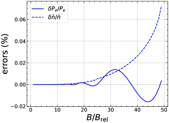
Figure 1: Relative errors (in %) of the approximate analytical expansions (14) and (2.2) for the baryon number density $\bar{n}$ (dashed line) and electron pressure $P_{e}$ (solid line), respectively, as a function of the magnetic field strength $B_{\star}=B/B_{\rm rel}$ with $\gamma_{e}=10$. The errors are obtained by taking the difference between the approximate and exact results and dividing by the exact result. All electrons are confined to the lowest Landau–Rabi level at $B_{\star}=(\gamma_{e}^{2}-1)/2=49.5$.

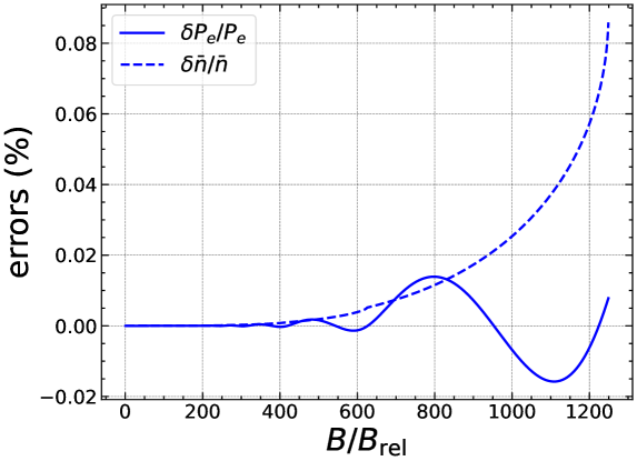
Figure 2: Same as Figure 1 for $\gamma_{e}=50$. All electrons are confined to the lowest Landau–Rabi level at $B_{\star}=(\gamma_{e}^{2}-1)/2=1249.5$.

2.3 Strongly Quantizing Magnetic Field

The magnetic field is strongly quantizing if all electrons lie in the lowest Landau-Rabi level. Setting $\nu_{\rm max}=0$ in Equations (5) and (8) leads to the following expression for the pressure and mean baryon number density:

$$P =\frac{B_{\star}m_{e}c^{2}}{4\pi^{2}\lambda_{e}^{3}}\biggl{[}\gamma_{e}\sqrt{\gamma_{e}^{2}-1}-\ln\left(\sqrt{\gamma_{e}^{2}-1}+\gamma_{e}\right)$$

$$+\frac{C_{M}\alpha}{3}\left(\frac{16B_{\star}Z^{2}}{3\pi}\right)^{1/3}\left(\gamma_{e}^{2}-1\right)^{2/3}\biggr{]}\,,$$ (22)

$$\bar{n}=\frac{B_{\star}}{2\pi^{2}\lambda_{e}^{3}}\frac{A}{Z}\sqrt{\gamma_{e}^{2}-1}\,.$$ (23)

These expressions hold if

$$\gamma_{e}<\sqrt{1+2B_{\star}}\,,$$ (24)

or equivalently if

$$n_{e}<\frac{B_{\star}^{3/2}}{\sqrt{2}\pi^{2}\lambda_{e}^{3}}\,,$$ (25)

using Equations (7) and (8).

3 Initial Composition of Magnetar Crusts

Assuming the crust is initially in a full thermodynamic equilibrium in the presence of some magnetic field, the composition is found by minimizing the Gibbs free energy per nucleon, which coincides with the baryon chemical potential (see, e.g., Appendix A in Chamel and Fantina (2015)):

$$\mu=\frac{\mathcal{E}+P}{\bar{n}}=\frac{M^{\prime}(A,Z,B_{\star})c^{2}}{A}+\frac{Z}{A}m_{e}c^{2}\biggl{[}\gamma_{e}-1+\frac{4}{3}C_{M}\left(\frac{4\pi}{3}\right)^{1/3}\alpha\lambda_{e}n_{e}^{1/3}Z^{2/3}\biggr{]}\,.$$ (26)

This minimization can be performed very efficiently following the iterative approach proposed in Chamel (2020); Chamel and Stoyanov (2020). Freely available computer codes in the limiting cases $\nu_{\rm max}\rightarrow+\infty$ and $\nu_{\rm max}=0$ can be found in Chamel (2020); Chamel and Stoyanov (2020).

3.1 Interface between Adjacent Crustal Layers

The pressure $P_{1\rightarrow 2}$ associated with the transition from a crustal layer made of nuclei ($A_{1}$, $Z_{1}$) to a denser layer made of nuclei ($A_{2}$, $Z_{2}$) is determined by the equilibrium condition

$$\mu(A_{1},Z_{1},P_{1\rightarrow 2})=\mu(A_{2},Z_{2},P_{1\rightarrow 2})\,,$$ (27)

which can be approximately written as Chamel (2020)

$$\gamma_{e}+C_{M}\,\alpha\lambda_{e}F(Z_{1},A_{1};Z_{2},A_{2})\left(\frac{4\pi n_{e}}{3}\right)^{1/3}=\gamma_{e}^{1\rightarrow 2}\,,$$ (28)

$$F(Z_{1},A_{1};Z_{2},A_{2})\equiv\left(\frac{4}{3}\frac{Z_{1}^{2/3}Z_{1}}{A_{1}}-\frac{1}{3}\frac{Z_{1}^{2/3}Z_{2}}{A_{2}}-\frac{Z_{2}^{2/3}Z_{2}}{A_{2}}\right)\left(\frac{Z_{1}}{A_{1}}-\frac{Z_{2}}{A_{2}}\right)^{-1}\,,$$ (29)

$$\gamma_{e}^{1\rightarrow 2}\equiv\biggl{[}\frac{M^{\prime}(A_{2},Z_{2},B_{\star})}{A_{2}m_{e}}-\frac{M^{\prime}(A_{1},Z_{1},B_{\star})}{A_{1}m_{e}}\biggr{]}\left(\frac{Z_{1}}{A_{1}}-\frac{Z_{2}}{A_{2}}\right)^{-1}+1\,.$$ (30)

The bottom of the outer crust is defined by the depth at which neutrons start to drip out of nuclei. The corresponding electron Fermi energy obeys an equation similar to Equation (28), the function $F(Z_{1},A_{1};Z_{2},A_{2})$ being replaced by $(4/3)Z^{2/3}$ and $\gamma_{e}^{1\rightarrow 2}$ by Chamel et al. (2015)

$$\gamma_{e}^{\rm drip}\equiv\frac{-M^{\prime}(A,Z,B_{\star})c^{2}+Am_{n}c^{2}}{Zm_{e}c^{2}}+1\,,$$ (31)

where $m_{n}$ is the neutron mass.

The threshold condition (28) takes formally the same form with and without magnetic fields. However, the solutions do depend on $B_{\star}$ through the relation between $\gamma_{e}$ and $n_{e}$, and potentially also through the ion masses.

3.2 No Magnetic Field

In the absence of magnetic field $B_{\star}=0$, the solution of Equation (28) reads Chamel (2020)

$$x_{r} = \gamma_{e}^{1\rightarrow 2}\Biggl{\{}\sqrt{1-\Biggl{[}1-\tilde{F}(Z_{1},A_{1};Z_{2},A_{2})^{2}\Biggr{]}/(\gamma_{e}^{1\rightarrow 2})^{2}}-\tilde{F}(Z_{1},A_{1};Z_{2},A_{2})\Biggr{\}}$$ (32)

$$\times\Biggl{[}1-\tilde{F}(Z_{1},A_{1};Z_{2},A_{2})^{2}\Biggr{]}^{-1}\,,$$

with

$$\tilde{F}(Z_{1},A_{1};Z_{2},A_{2})\equiv\left(\frac{4}{9\pi}\right)^{1/3}C_{M}\alpha F(Z_{1},A_{1};Z_{2},A_{2})\,.$$ (33)

This solution exists only if $\tilde{F}(Z_{1},A_{1};Z_{2},A_{2})\geq-1$.

The mean baryon number density $\bar{n}_{1}^{\rm max}$ up to which nuclei $(A_{1},Z_{1})$ are present and the transition pressure $P_{1\rightarrow 2}$ are then given by Equations (19) and (20) respectively.

3.3 Strongly Quantizing Magnetic Field

The solution of Equation (28) was also found in the limit of a strongly quantizing magnetic field Chamel and Stoyanov (2020). Introducing

$$\bar{F}(Z_{1},A_{1};Z_{2},A_{2};B_{\star})\equiv\frac{1}{3}C_{M}\alpha F(Z_{1},A_{1};Z_{2},A_{2})\left(\frac{2B_{\star}}{3\pi}\right)^{1/3}\,,$$ (34)

$$\upsilon\equiv\frac{\gamma_{e}^{1\rightarrow 2}}{2|\bar{F}(Z_{1},A_{1};Z_{2},A_{2};B_{\star})|^{3/2}}\,,$$ (35)

the electron Fermi energy at the crustal interface is given by the following formulas:

• $\gamma_{e}^{1\rightarrow 2}>0$ and $\bar{F}(Z_{1},A_{1};Z_{2},A_{2};B_{\star})>0$

  $$\gamma_{e}=8\bar{F}(Z_{1},A_{1};Z_{2},A_{2};B_{\star})^{3/2}\,{\rm sinh}^{3}\left(\frac{1}{3}{\rm arcsinh~{}}\upsilon\right)\,,$$ (36)

• $\gamma_{e}^{1\rightarrow 2}>0$ and $\bar{F}(Z_{1},A_{1};Z_{2},A_{2};B_{\star})<0$

  $$\gamma_{e}=\begin{cases}8|\bar{F}(Z_{1},A_{1};Z_{2},A_{2};B_{\star})|^{3/2}\,{\rm cosh}^{3}\left(\frac{1}{3}{\rm arccosh~{}}\upsilon\right)&\text{if}\ \upsilon\geq 1\,,\\ 8|\bar{F}(Z_{1},A_{1};Z_{2},A_{2};B_{\star})|^{3/2}\,\cos^{3}\left(\frac{1}{3}\arccos\upsilon\right)&\text{if}\ 0\leq\upsilon<1\,.\end{cases}$$ (37)

• $\gamma_{e}^{1\rightarrow 2}<0$ and $\bar{F}(Z_{1},A_{1};Z_{2},A_{2};B_{\star})<0$

  $$\gamma_{e}=8|\bar{F}(Z_{1},A_{1};Z_{2},A_{2};B_{\star})|^{3/2}\,\cos^{3}\theta_{k}\ \ \text{if}\ -1<\upsilon\leq 0\,,$$ (38)

  $$\theta_{k}\equiv\frac{1}{3}\arccos\upsilon+\frac{2\pi k}{3}\ \ \text{and}\ k=0,2\,.$$ (39)

The mean baryon number density $\bar{n}_{1}^{\rm max}$ up to which nuclei $(A_{1},Z_{1})$ are present and the transition pressure $P_{1\rightarrow 2}$ are then given by Equations (23) and (2.3), respectively. In the case $\gamma_{e}^{1\rightarrow 2}<0$, the physically admissible solution among $k=0$ and $k=2$ is the one yielding the lowest transition pressure $P_{1\rightarrow 2}$ satisfying the conditions $\gamma_{e}>1$ and $\bar{n}_{2}^{\rm min}\geq\bar{n}_{1}^{\rm max}$.

Let us recall that these solutions are only valid under the assumption $\nu_{\rm max}=0$, which translates into a lower bound for the magnetic field $B_{\star}\geq B^{1\rightarrow 2}_{\star}$. To find $B^{1\rightarrow 2}_{\star}$, we substitute Equations (24) and (25) in Equation (28). This leads to

$$B^{1\rightarrow 2}_{\star}=\frac{(\gamma_{e}^{1\rightarrow 2})^{2}}{2}\biggl{[}1+\frac{C_{M}\alpha}{(3\pi)^{1/3}}F(Z_{1},A_{1};Z_{2},A_{2})\biggr{]}^{-2}\,.$$ (40)

We have assumed $B^{1\rightarrow 2}_{\star}\gg 1$ so that $\gamma_{e}\approx\sqrt{2B^{1\rightarrow 2}_{\star}}$.

3.4 Intermediate Magnetic Fields

Approximate analytical solutions can also be found in the intermediate regime. Remarking that the magnetic field enters explicitly in Equation (28) only through the small electrostatic correction, the threshold electron Fermi energy $\gamma_{e}$ is still approximately given by the solution in the absence of magnetic fields, Equations (21) and (32). However, the density and the pressure are now given by Equations (14) and (2.2), respectively. As shown in Section 2.2, these expansions in the weakly quantizing limit $\nu_{\rm max}\gg 1$ (including the absence of magnetic field as a limiting case) actually remain very precise for $\nu_{\rm max}\sim 1$ and even at the onset of the strongly quantizing regime $\nu_{\rm max}=0$. Combining the solutions thus obtained with those presented in Section 3.3, the full range of possible initial magnetic field strengths can be treated analytically.

4 Magnetic Field Decay and Electron Captures

4.1 Onset of Electron Captures

The initial magnetic field decays on a very long time scale, say of the typical order of millions of years Pons and Viganò (2019). The compression of the crust thus occurs very slowly. When the pressure of a matter element reaches some value $P_{\beta}(A,Z,B_{\star})$, the capture of an electron by nuclei $(A,Z)$ (in their ground state) opens. The daughter nuclei may be in an excited state.

The onset of electron captures by nuclei $(A,Z)$ is formally determined by the same condition irrespective of the magnetic field strength by requiring the constancy of the Gibbs free energy per nucleon at fixed temperature and pressure Chamel and Fantina (2015). The threshold electron Fermi energy is found to the first order in the fine-structure constant $\alpha$ from the condition:

$$\gamma_{e}+C_{M}\left(\frac{4\pi n_{e}}{3}\right)^{1/3}\alpha\lambda_{e}F(Z)=\gamma_{e}^{\beta}\,,$$ (41)

$$F(Z)\equiv Z^{5/3}-(Z-1)^{5/3}+\frac{1}{3}Z^{2/3}\,,$$ (42)

$$\gamma_{e}^{\beta}\equiv-\frac{Q_{\rm EC}(A,Z,B_{\star})}{m_{e}c^{2}}+1\,,$$ (43)

where we have introduced the $Q$-value (in vacuum) associated with electron capture by nuclei ($A,Z$):

$$Q_{\rm EC}(A,Z,B_{\star})=M^{\prime}(A,Z,B_{\star})c^{2}-M^{\prime}(A,Z-1,B_{\star})c^{2}-E_{\rm ex}(A,Z-1,B_{\star})\,.$$ (44)

These $Q$-values can be obtained from the tabulated $Q$-values of $\beta$ decay by the following relation:

$$Q_{\rm EC}(A,Z,B_{\star})=-Q_{\beta}(A,Z-1,B_{\star})-E_{\rm ex}(A,Z-1,B_{\star})\,.$$ (45)

Here, $E_{\rm ex}(A,Z-1,B_{\star})$ denotes the excitation energy of the daughter nucleus. Transitions to the ground state can be considered by setting $E_{\rm ex}(A,Z-1,B_{\star})=0$.

4.2 No Magnetic Field

In the absence of magnetic fields, the threshold condition (41) can be solved exactly Chamel and Fantina (2016):

$$\gamma_{e}=\sqrt{1+(x_{r}^{\beta})^{2}}\,,$$ (46)

$$x^{\beta}_{r}=\gamma_{e}^{\beta}\Biggl{\{}\sqrt{1-\biggl{[}1-\tilde{F}(Z)^{2}\biggr{]}/(\gamma_{e}^{\beta})^{2}}-\tilde{F}(Z)\Biggr{\}}\Biggl{[}1-\tilde{F}(Z)^{2}\Biggr{]}^{-1}\,,$$ (47)

$$\tilde{F}(Z)\equiv C_{M}\left(\frac{4}{9\pi}\right)^{1/3}\alpha F(Z)\,.$$ (48)

The pressure $P_{\beta}(A,Z)$ and the density $\bar{n}_{\beta}(A,Z)$ at the onset of electron captures are then given by Equations (20) and (19), respectively.

4.3 Intermediate Magnetic Field

For $\nu_{\rm max}>0$, the density and the pressure are obtained by substituting the solution (46) for the threshold electron Fermi energy in the absence of magnetic field in Equations (14) and (2.2), respectively.

4.4 Strongly Quantizing Magnetic Field

In the strongly quantizing regime ($\nu_{\text{max}}=0$), Equation (41) can be solved exactly from the general analytical solutions given in Section 3.3. Introducing

$$\bar{F}(Z,B_{\star})\equiv\frac{1}{3}C_{M}\alpha F(Z)\left(\frac{2B_{\star}}{3\pi}\right)^{1/3}<0\,,$$ (49)

$$\upsilon\equiv\frac{\gamma_{e}^{\beta}}{2|\bar{F}(Z,B_{\star})|^{3/2}}\,,$$ (50)

remarking that $\gamma_{e}^{\beta}>1$, the solutions are given by the following formulas:

$$\gamma_{e}=\begin{cases}8|\bar{F}(Z,B_{\star})|^{3/2}\,{\rm cosh}^{3}\left(\frac{1}{3}{\rm arccosh\,}\upsilon\right)&\text{if}\ \upsilon\geq 1\,,\\ 8|\bar{F}(Z,B_{\star})|^{3/2}\,\cos^{3}\left(\frac{1}{3}\arccos\upsilon\right)&\text{if}\ 0\leq\upsilon<1\,.\end{cases}$$ (51)

The threshold pressure and density are respectively given by Equations (2.3) and (23).

Let us recall that this solution is only valid under the assumption $\nu_{\rm max}=0$, which translates into a lower bound for the magnetic field $B_{\star}\geq B_{\star}^{\beta}$. To find $B_{\star}^{\beta}$, we substitute Equations (24) and (25) in Equation (41). This leads to

$$B_{\star}^{\beta}=\frac{(\gamma_{e}^{\beta})^{2}}{2}\biggl{[}1+\frac{C_{M}\alpha}{(3\pi)^{1/3}}F(Z)\biggr{]}^{-2}\,.$$ (52)

We have assumed $B^{\beta}_{\star}\gg 1$ so that $\gamma_{e}\approx\sqrt{2B_{\star}^{\beta}}$.

4.5 Heat Released

The first electron capture does not release any significant heat since it essentially proceeds in quasiequilibrium. However, the daughter nuclei (possibly in some excited state) are generally unstable and capture a second electron off-equilibrium thus depositing some heat at the same pressure $P_{\beta}(A,Z,B_{\star})$. Ignoring the fraction of energy carried away by neutrinos, the maximum amount of heat per nucleus $(A,Z)$ is given by

$$\mathcal{Q}(A,Z,B_{\star})=\mu(A,Z,B_{\star})-\mu(A,Z-2,B_{\star})\,.$$ (53)

It is to be understood that the baryon chemical potentials must be evaluated at the same pressure. Expressing the electron Fermi energy associated with nuclei $(A,Z-2)$ as $\gamma_{e}+\delta\gamma_{e}$ with $\gamma_{e}$ given by the solution of Equation (41), and expanding the pressure to the first order in $\delta\gamma_{e}$ leads to

$$\delta\gamma_{e}\approx\frac{1}{3}C_{M}\alpha\lambda_{e}\left(\frac{4\pi n_{e}}{3}\right)^{1/3}\left[Z^{2/3}-(Z-2)^{2/3}\right]\,.$$ (54)

We have made use of the Gibbs–Duhem relation $dP_{e}=n_{e}m_{e}c^{2}d\gamma_{e}$ and we have neglected terms of order $\alpha\delta\gamma_{e}$. Substituting Equation (54) in Equation (53) and eliminating $\gamma_{e}$ using Equation (41) lead to the following expression for the heat released per nucleus (keeping as before first-order terms):

$$\mathcal{Q}(A,Z,B_{\star}) \approx\mathcal{Q}^{(0)}(A,Z,B_{\star})$$ (55)

$$-C_{M}\alpha m_{e}c^{2}\lambda_{e}\left(\frac{4\pi A}{3Z}\bar{n}\right)^{1/3}\biggl{[}Z^{5/3}+(Z-2)^{5/3}-2(Z-1)^{5/3}\biggr{]}\,,$$

where the zeroth-order term is determined by nuclear data alone

$$\mathcal{Q}^{(0)}(A,Z,B_{\star}) \equiv 2M^{\prime}(A,Z-1,B_{\star})c^{2}+2E_{\rm ex}(A,Z-1,B_{\star})$$ (56)

$$-M^{\prime}(A,Z-2,B_{\star})c^{2}-M^{\prime}(A,Z,B_{\star})c^{2}\,.$$

Apart from the small electrostatic correction (the term proportional to the structure constant $C_{M}$), the maximum heat released by electron captures is thus independent of whether the crust is solid or liquid. Unless $B\gtrsim 10^{17}$ G Peña Arteaga et al. (2011), the structure of nuclei remains essentially unchanged in the presence of a magnetic field so that $\mathcal{Q}(A,Z,B_{\star})\approx\mathcal{Q}(A,Z)$.

To estimate the heat in Equation (53), we implicitly assumed $\mu(A,Z-2,P_{\beta},B_{\star})<\mu(A,Z,P_{\beta},B_{\star})$, which generally holds for even $A$ nuclei, but not necessarily for odd $A$ nuclei. In the latter case, we typically have $Q_{\beta}(A,Z-1,B_{\star})<Q_{\beta}(A,Z-2,B_{\star})$. Using Equation (43), this implies that $\gamma_{e}^{\beta}(A,Z)<\gamma_{e}^{\beta}(A,Z-1)$. In other words, as the pressure reaches $P_{\beta}(A,Z,B_{\star})$, the nucleus ($A,Z$) decays, but the daughter nucleus ($A,Z-1$) is actually stable against electron capture, and therefore, no heat is released $\mathcal{Q}(A,Z,B_{\star})=0$. The daughter nucleus sinks deeper in the crust and only captures a second electron in quasi-equilibrium at pressure $P_{\beta}(A,Z-1,B_{\star})>P_{\beta}(A,Z,B_{\star})$.

4.6 Neutron Delayed Emission

As discussed in Chamel et al. (2015); Fantina et al. (2016), the first electron capture by the nucleus $(A,Z)$ may be accompanied by the emission of $\Delta N>0$ neutrons. The corresponding pressure $P_{\beta n}$ and baryon density $n_{\beta n}$ are obtained from similar expressions as for electron captures except that the threshold electron Fermi energy $\gamma_{e}^{\beta}$ is now replaced by

$$\gamma_{e}^{\beta n}=\frac{M^{\prime}(A-\Delta N,Z-1)c^{2}+E_{\rm ex}(A-\Delta N,Z-1)-M^{\prime}(A,Z)c^{2}+\Delta Nm_{n}c^{2}}{m_{e}c^{2}}+1\,.$$ (57)

Neutron emission will thus occur whenever $\gamma_{e}^{\beta n}(A,Z)<\gamma_{e}^{\beta}(A,Z)$.

5 Results and Discussions

5.1 Initial Composition of the Outer Crust

The initial composition of the outer crust of a magnetar was determined in Mutafchieva et al. (2019) but only for a few selected magnetic field strengths, namely $B_{\star}=1000$, 2000, and  3000. We have extended the calculations to the whole range of magnetic field strengths ranging from $B=0$ to $B=10^{17}$ G. To this end, we have used the experimental atomic masses from the 2016 Atomic Mass Evaluation Wang et al. (2017) supplemented with the same microscopic atomic mass table HFB-24 Goriely et al. (2013) from the BRUSLIB database Xu et al. (2013). The functional BSk24 underlying the model HFB-24 was also adopted to calculate the equation of state of the inner crust of a magnetar Mutafchieva et al. (2019). This same functional was also applied to construct a unified equation of state for unmagnetized neutron stars Pearson et al. (2018, 2020); Pearson and Chamel (2022), and to calculate superfluid properties Allard and Chamel (2021). Results are publicly available on CompOSE. This equation of state is consistent with the constraints inferred from analyses of the gravitational-wave signal from the binary neutron-star merger GW170817 and of its electromagnetic counterpart Perot et al. (2019). As shown in Mutafchieva et al. (2019), the magnetic field has a negligible impact on the equation of the state of the inner crust and core of magnetars unless it exceeds about $10^{17}$ G.

Depending on the strength of the magnetic field when the magnetar was born, different nuclides are expected to be produced in the outer crust. Changes in the composition compared to that obtained in Pearson et al. (2018) in the absence of the magnetic field are summarized in Tables 2 and 3. The mean baryon number densities and the pressure at the interface between adjacent crustal layers can be calculated for any magnetic field using the analytical formulas given in Section 3. The only nuclear inputs are embedded in the parameter $\gamma_{e}^{1\rightarrow 2}$ defined by Equation (30). Values for this parameter are indicated in Table 5 for all possible transitions.

Table 1: Magnetic field strength $B_{\star}=B/B_{\rm rel}$ for the appearance (+) or the disappearance ($-$) of a nuclide in the outer crust of a magnetar.

Nuclide	$\boldsymbol{B_{\star}}$
66Ni($-$)	67
88Sr(+)	858
126Ru(+)	1023
80Ni($-$)	1072
128Pd(+)	1249
78Ni($-$)	1416
64Ni($-$)	1669

Table 2: Cont.

Nuclide	$\boldsymbol{B_{\star}}$
124Zr(+)	1872
121Y($-$)	1907
132Sn(+)	1986
80Ni($-$)	2087

Table 3: Sequence of equilibrium nuclides with increasing depth (from top to bottom) in the outer crust of a magnetar for different magnetic field strengths. The first row indicates values of $B_{\star}=B/B_{\rm rel}$ associated with a change of composition. Results are valid up to $B_{\star}=2087$.

	67	858	1023	1072	1249	1416	1669	1872	1907	1986
56Fe	56Fe	56Fe	56Fe	56Fe	56Fe	56Fe	56Fe	56Fe	56Fe	56Fe
62Ni	62Ni	62Ni	62Ni	62Ni	62Ni	62Ni	62Ni	62Ni	62Ni	62Ni
64Ni	64Ni	64Ni	64Ni	64Ni	64Ni	64Ni	–	–	–	–
66Ni	–	–	–	–	–	–	–	–	–	–
–	–	88Sr	88Sr	88Sr	88Sr	88Sr	88Sr	88Sr	88Sr	88Sr
86Kr	86Kr	86Kr	86Kr	86Kr	86Kr	86Kr	86Kr	86Kr	86Kr	86Kr
84Se	84Se	84Se	84Se	84Se	84Se	84Se	84Se	84Se	84Se	84Se
82Ge	82Ge	82Ge	82Ge	82Ge	82Ge	82Ge	82Ge	82Ge	82Ge	82Ge
–	–	–	–	–	–	–	–	–	–	132Sn
80Zn	80Zn	80Zn	80Zn	80Zn	80Zn	80Zn	80Zn	80Zn	80Zn	80Zn
78Ni	78Ni	78Ni	78Ni	78Ni	78Ni	–	–	–	–	–
80Ni	80Ni	80Ni	80Ni	–	–	–	–	–	–	–
–	–	–	–	–	128Pd	128Pd	128Pd	128Pd	128Pd	128Pd
–	–	–	126Ru	126Ru	126Ru	126Ru	126Ru	126Ru	126Ru	126Ru
124Mo	124Mo	124Mo	124Mo	124Mo	124Mo	124Mo	124Mo	124Mo	124Mo	124Mo
122Zr	122Zr	122Zr	122Zr	122Zr	122Zr	122Zr	122Zr	122Zr	122Zr	122Zr
–	–	–	–	–	–	–	–	124Zr	124Zr	124Zr
121Y	121Y	121Y	121Y	121Y	121Y	121Y	121Y	121Y	–	–
120Sr	120Sr	120Sr	120Sr	120Sr	120Sr	120Sr	120Sr	120Sr	120Sr	120Sr
122Sr	122Sr	122Sr	122Sr	122Sr	122Sr	122Sr	122Sr	122Sr	122Sr	122Sr
124Sr	124Sr	124Sr	124Sr	124Sr	124Sr	124Sr	124Sr	124Sr	124Sr	124Sr

Table 4: Values of the nuclear parameter $\gamma_{e}^{1\rightarrow 2}$ from which the pressure and the densities at the boundary between adjacent layers in the outer crust of a magnetar can be calculated.

$\boldsymbol{\gamma_{e}^{1\rightarrow 2}}$	Interface
1.8908	${}^{56}\mathrm{Fe}$ – ${}^{62}\mathrm{Ni}$
4.8972	${}^{62}\mathrm{Ni}$ – ${}^{64}\mathrm{Ni}$
8.6863	${}^{62}\mathrm{Ni}$ – ${}^{88}\mathrm{Sr}$
8.1312	${}^{64}\mathrm{Ni}$ – ${}^{66}\mathrm{Ni}$
9.3317	${}^{64}\mathrm{Ni}$ – ${}^{86}\mathrm{Kr}$
18.098	${}^{64}\mathrm{Ni}$ – ${}^{88}\mathrm{Sr}$
12.155	${}^{66}\mathrm{Ni}$ – ${}^{86}\mathrm{Kr}$
10.044	${}^{86}\mathrm{Kr}$ – ${}^{84}\mathrm{Se}$
5.5622	${}^{88}\mathrm{Sr}$ – ${}^{86}\mathrm{Kr}$
15.330	${}^{84}\mathrm{Se}$ – ${}^{82}\mathrm{Ge}$
20.519	${}^{82}\mathrm{Ge}$ – ${}^{80}\mathrm{Zn}$
38.310	${}^{82}\mathrm{Ge}$ – ${}^{132}\mathrm{Sn}$
25.926	${}^{80}\mathrm{Zn}$ – ${}^{78}\mathrm{Ni}$

Table 5: Cont.

$\boldsymbol{\gamma_{e}^{1\rightarrow 2}}$	Interface
37.083	${}^{80}\mathrm{Zn}$ – ${}^{128}\mathrm{Pd}$
$-33.289$	${}^{132}\mathrm{Sn}$ – ${}^{80}\mathrm{Zn}$
32.978	${}^{78}\mathrm{Ni}$ – ${}^{80}\mathrm{Ni}$
$-409.21$	${}^{78}\mathrm{Ni}$ – ${}^{128}\mathrm{Pd}$
48.055	${}^{78}\mathrm{Ni}$ – ${}^{126}\mathrm{Ru}$
45.122	${}^{80}\mathrm{Ni}$ – ${}^{124}\mathrm{Mo}$
218.54	${}^{80}\mathrm{Ni}$ – ${}^{126}\mathrm{Ru}$
30.039	${}^{128}\mathrm{Pd}$ – ${}^{126}\mathrm{Ru}$
32.010	${}^{126}\mathrm{Ru}$ – ${}^{124}\mathrm{Mo}$
37.441	${}^{124}\mathrm{Mo}$ – ${}^{122}\mathrm{Zr}$
40.352	${}^{122}\mathrm{Zr}$ – ${}^{121}\mathrm{Y}$
42.293	${}^{122}\mathrm{Zr}$ – ${}^{124}\mathrm{Zr}$
1.8541	${}^{124}\mathrm{Zr}$ – ${}^{121}\mathrm{Y}$
39.031	${}^{124}\mathrm{Zr}$ – ${}^{120}\mathrm{Sr}$
40.786	${}^{121}\mathrm{Y}$ – ${}^{120}\mathrm{Sr}$
44.857	${}^{120}\mathrm{Sr}$ – ${}^{122}\mathrm{Sr}$
47.747	${}^{122}\mathrm{Sr}$ – ${}^{124}\mathrm{Sr}$

5.2 Heating

We have estimated the heat released by electron captures and their location using the experimental atomic masses and the $Q_{\beta}$ values (including the recommended ones) from the 2016 Atomic Mass Evaluation Wang et al. (2017) supplemented with the atomic mass model HFB-24 Goriely et al. (2013). We have taken excitation energies from the Nuclear Data section of the International Atomic Energy Agency website following the Gamow–Teller selection rules, namely that the parity of the final state is the same as that of the initial state, whereas the total angular momentum $J$ can either remain unchanged or vary by $\pm\hbar$ (excluding transitions from $J=0$ to $J=0$).

The threshold density and pressure for the onset of each electron capture, as well as the amount of heat deposited, can be calculated for any magnetic field strength from the analytical formulas presented in Section 4 using the parameters indicated in Table 7 for ground-state to ground-state transitions, in Table 8 for ground-state to excited state transitions, and in Table 9 for transitions involving light elements that could have been accreted from the interstellar medium. Full numerical results are freely available in Chamel and Fantina (2022).

Table 6: Values of the nuclear parameters $\gamma_{e}^{\beta}$ and $\mathcal{Q}^{(0)}$ (considering ground-state to ground-state transitions) from which the threshold density and pressure for the onset of electron captures, as well as the heat released can be calculated. The symbol ($\star$) is used to distinguish reactions for which theoretical atomic masses were needed.

$\boldsymbol{\gamma_{e}^{\beta}}$	Reaction	$\boldsymbol{\mathcal{Q}^{(0)}}$ (MeV)
8.232	${}^{56}\mathrm{Fe}\rightarrow{}^{56}\mathrm{Cr}-2e^{-}+2\nu_{e}$	2.069
18.867	${}^{56}\mathrm{Cr}\rightarrow{}^{56}\mathrm{Ti}-2e^{-}+2\nu_{e}$	2.295
29.313	${}^{56}\mathrm{Ti}\rightarrow{}^{56}\mathrm{Ca}-2e^{-}+2\nu_{e}$	3.514
43.710	${}^{56}\mathrm{Ca}\rightarrow{}^{56}\mathrm{Ar}-2e^{-}+2\nu_{e}\ (\star)$	2.045
11.415	${}^{62}\mathrm{Ni}\rightarrow{}^{62}\mathrm{Fe}-2e^{-}+2\nu_{e}$	2.776
21.262	${}^{62}\mathrm{Fe}\rightarrow{}^{62}\mathrm{Cr}-2e^{-}+2\nu_{e}$	2.725
31.174	${}^{62}\mathrm{Cr}\rightarrow{}^{62}\mathrm{Ti}-2e^{-}+2\nu_{e}$	2.442
41.470	${}^{62}\mathrm{Ti}\rightarrow{}^{62}\mathrm{Ca}-2e^{-}+2\nu_{e}\ (\star)$	2.490

Table 7: Cont.

$\boldsymbol{\gamma_{e}^{\beta}}$	Reaction	$\boldsymbol{\mathcal{Q}^{(0)}}$ (MeV)
15.299	${}^{64}\mathrm{Ni}\rightarrow{}^{64}\mathrm{Fe}-2e^{-}+2\nu_{e}$	2.484
24.445	${}^{64}\mathrm{Fe}\rightarrow{}^{64}\mathrm{Cr}-2e^{-}+2\nu_{e}$	2.471
34.581	${}^{64}\mathrm{Cr}\rightarrow{}^{64}\mathrm{Ti}-2e^{-}+2\nu_{e}$	1.865
19.782	${}^{66}\mathrm{Ni}\rightarrow{}^{66}\mathrm{Fe}-2e^{-}+2\nu_{e}$	3.257
27.062	${}^{66}\mathrm{Fe}\rightarrow{}^{66}\mathrm{Cr}-2e^{-}+2\nu_{e}$	1.287
38.397	${}^{66}\mathrm{Cr}\rightarrow{}^{66}\mathrm{Ti}-2e^{-}+2\nu_{e}\ (\star)$	3.540
15.938	${}^{86}\mathrm{Kr}\rightarrow{}^{86}\mathrm{Se}-2e^{-}+2\nu_{e}$	2.504
23.585	${}^{86}\mathrm{Se}\rightarrow{}^{86}\mathrm{Ge}-2e^{-}+2\nu_{e}$	1.979
30.980	${}^{86}\mathrm{Ge}\rightarrow{}^{86}\mathrm{Zn}-2e^{-}+2\nu_{e}\ (\star)$	2.310
38.926	${}^{86}\mathrm{Zn}\rightarrow{}^{86}\mathrm{Ni}-2e^{-}+2\nu_{e}\ (\star)$	2.320
20.754	${}^{84}\mathrm{Se}\rightarrow{}^{84}\mathrm{Ge}-2e^{-}+2\nu_{e}$	2.389
28.517	${}^{84}\mathrm{Ge}\rightarrow{}^{84}\mathrm{Zn}-2e^{-}+2\nu_{e}$	1.903
36.362	${}^{84}\mathrm{Zn}\rightarrow{}^{84}\mathrm{Ni}-2e^{-}+2\nu_{e}\ (\star)$	2.390
25.431	${}^{82}\mathrm{Ge}\rightarrow{}^{82}\mathrm{Zn}-2e^{-}+2\nu_{e}$	1.868
34.256	${}^{82}\mathrm{Zn}\rightarrow{}^{82}\mathrm{Ni}-2e^{-}+2\nu_{e}\ (\star)$	2.154
44.640	${}^{82}\mathrm{Ni}\rightarrow{}^{82}\mathrm{Fe}-2e^{-}+2\nu_{e}\ (\star)$	2.080
31.233	${}^{80}\mathrm{Zn}\rightarrow{}^{80}\mathrm{Ni}-2e^{-}+2\nu_{e}$	1.879
39.435	${}^{78}\mathrm{Ni}\rightarrow{}^{78}\mathrm{Fe}-2e^{-}+2\nu_{e}\ (\star)$	2.070
41.842	${}^{124}\mathrm{Mo}\rightarrow{}^{124}\mathrm{Zr}-2e^{-}+2\nu_{e}\ (\star)$	2.920
42.722	${}^{122}\mathrm{Zr}\rightarrow{}^{122}\mathrm{Sr}-2e^{-}+2\nu_{e}\ (\star)$	0.790
11.397	${}^{88}\mathrm{Sr}\rightarrow{}^{88}\mathrm{Kr}-2e^{-}+2\nu_{e}$	2.395
18.564	${}^{88}\mathrm{Kr}\rightarrow{}^{88}\mathrm{Se}-2e^{-}+2\nu_{e}$	2.144
26.761	${}^{88}\mathrm{Se}\rightarrow{}^{88}\mathrm{Ge}-2e^{-}+2\nu_{e}$	2.582
34.601	${}^{88}\mathrm{Ge}\rightarrow{}^{88}\mathrm{Zn}-2e^{-}+2\nu_{e}\ (\star)$	2.740
36.695	${}^{126}\mathrm{Ru}\rightarrow{}^{126}\mathrm{Mo}-2e^{-}+2\nu_{e}\ (\star)$	1.860
34.444	${}^{128}\mathrm{Pd}\rightarrow{}^{128}\mathrm{Ru}-2e^{-}+2\nu_{e}\ (\star)$	2.290
28.662	${}^{132}\mathrm{Sn}\rightarrow{}^{132}\mathrm{Cd}-2e^{-}+2\nu_{e}$	1.987
33.237	${}^{132}\mathrm{Cd}\rightarrow{}^{132}\mathrm{Pd}-2e^{-}+2\nu_{e}\ (\star)$	2.863
38.084	${}^{132}\mathrm{Pd}\rightarrow{}^{132}\mathrm{Ru}-2e^{-}+2\nu_{e}\ (\star)$	2.940

Table 8: Same as in Table 7 but considering ground-state to excited state transitions (for which the excitation energy is experimentally known and $E_{\textrm{exc}}>0$).

$\boldsymbol{\gamma_{e}^{\beta}}$	Reaction	$\boldsymbol{\mathcal{Q}^{(0)}}$ (MeV)
8.448	${}^{56}\mathrm{Fe}\rightarrow{}^{56}\mathrm{Cr}-2e^{-}+2\nu_{e}$	2.290
12.405	${}^{62}\mathrm{Ni}\rightarrow{}^{62}\mathrm{Fe}-2e^{-}+2\nu_{e}$	3.788
20.726	${}^{86}\mathrm{Kr}\rightarrow{}^{86}\mathrm{Se}-2e^{-}+2\nu_{e}$	7.397
31.260	${}^{82}\mathrm{Ge}\rightarrow{}^{82}\mathrm{Zn}-2e^{-}+2\nu_{e}$	7.825
15.764	${}^{88}\mathrm{Sr}\rightarrow{}^{88}\mathrm{Kr}-2e^{-}+2\nu_{e}$	6.858
22.290	${}^{88}\mathrm{Kr}\rightarrow{}^{88}\mathrm{Se}-2e^{-}+2\nu_{e}$	5.951
31.010	${}^{132}\mathrm{Sn}\rightarrow{}^{132}\mathrm{Cd}-2e^{-}+2\nu_{e}$	4.387

Table 9: Same as in Tables 7 but considering reactions involving carbon and oxygen.

$\boldsymbol{\gamma_{e}^{\beta}}$	Reaction	$\boldsymbol{\mathcal{Q}^{(0)}}$ (MeV)
21.393	${}^{16}\mathrm{O}\rightarrow{}^{16}\mathrm{C}-2e^{-}+2\nu_{e}$	2.411
27.163	${}^{12}\mathrm{C}\rightarrow{}^{12}\mathrm{Be}-2e^{-}+2\nu_{e}$	1.661

To assess the reliability of our analytical treatment, we have numerically solved the exact threshold conditions $\mu(A,Z,n_{e})=\mu(A,Z-1,n_{e1})$ and $P(Z,n_{e})=P(Z-1,n_{e1})=P(Z-2,n_{e2})$ without any approximation, i.e., using Equations (5) and (8), to determine the exact values for the threshold pressure $P_{\beta}$ and baryon number density $\bar{n}_{\beta}$. The heat deposited is then calculated as $\mathcal{Q}=\mu(A,Z,n_{e})-\mu(A,Z-2,n_{e2})$. We have compared these exact results with the approximate analytical formulas. As an example, we focus on the electron capture by ⁵⁶Fe, considering the ground-state to ground-state transition. As shown in Figure 3, the quantum oscillations of the threshold density are correctly reproduced. The errors are found to be the largest for specific values of the magnetic field strength corresponding to exact fillings of Landau–Rabi levels and amount to a few percents, but drop by about an order of magnitude in the strongly quantizing regime, as shown in Figure 4. As previously discussed in Section 2.2, the expansion in the weakly quantizing regime is more reliable for the pressure than for the density. Indeed, the overall errors on the threshold pressure are significantly smaller, as can be observed in Figure 5. In the strongly quantizing regime, the errors on $P_{\beta}$ are of the same order as those on $\bar{n}_{\beta}$ and are displayed in Figure 6. The heat released, plotted in Figures 7 and 8, also exhibits quantum oscillations, though the amplitude is very small. To a first approximation, the heat is therefore essentially given by that in the absence of magnetic fields, as anticipated. The analytical formula for $\mathcal{Q}$ is found to be even more precise than formulas for the density and pressure. To check that these error estimates are not specific to the reaction considered, we have also analyzed the electron capture by ¹²²Zr, which is present in much deeper layers of the outer crust for all the magnetic field strengths. As can be observed in Figures 9–14, the analytical formulas remain very precise in this other case. We have examined other reactions and reached similar conclusions.

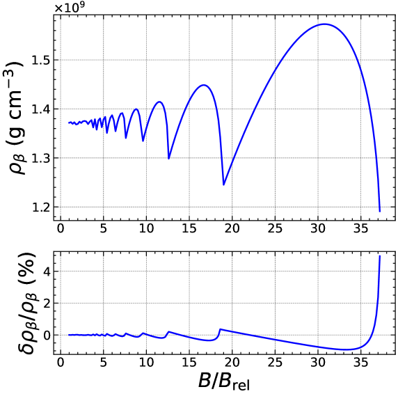
Figure 3: Top panel: Exact threshold density (in cgs units) for the onset of electron captures by ⁵⁶Fe as a function of the magnetic field strength $B_{\star}=B/B_{\rm rel}$ up to the onset of the strongly quantizing regime. Bottom panel: Relative error (in %) of the approximate analytical expression.

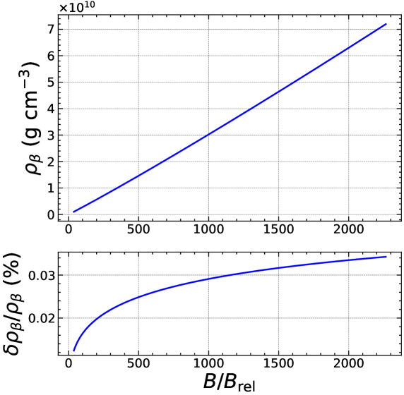
Figure 4: Same as Figure 3 in the strongly quantizing regime.

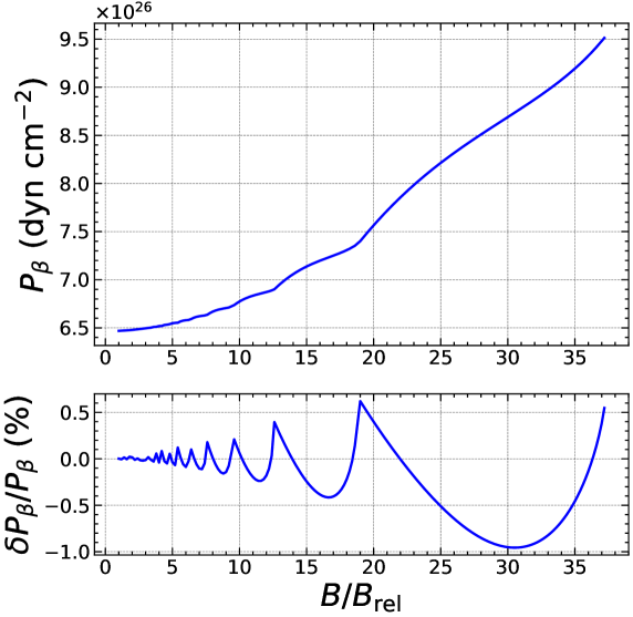
Figure 5: Top panel: Exact threshold pressure (in cgs units) for the onset of electron captures by ⁵⁶Fe as a function of the magnetic field strength $B_{\star}=B/B_{\rm rel}$ up to the onset of the strongly quantizing regime. Bottom panel: Relative error (in %) of the approximate analytical expression.

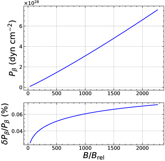
Figure 6: Same as Figure 5 in the strongly quantizing regime.

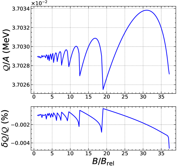
Figure 7: Top panel: Exact heat released per nucleon from electron captures by ⁵⁶Fe as a function of the magnetic field strength $B_{\star}=B/B_{\rm rel}$ up to the onset of the strongly quantizing regime. Bottom panel: Relative error (in %) of the approximate analytical expression.

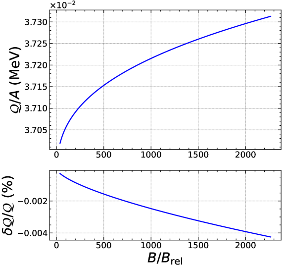
Figure 8: Same as Figure 7 in the strongly quantizing regime.

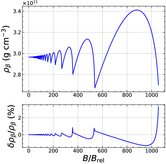
Figure 9: Top panel: Exact threshold density (in cgs units) for the onset of electron captures by ¹²²Zr as a function of the magnetic field strength $B_{\star}=B/B_{\rm rel}$ up to the onset of the strongly quantizing regime. Bottom panel: Relative error (in %) of the approximate analytical expression.

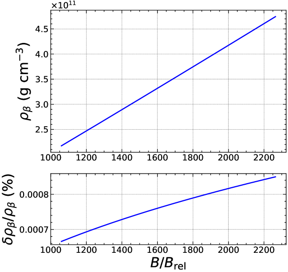
Figure 10: Same as Figure 9 in the strongly quantizing regime.

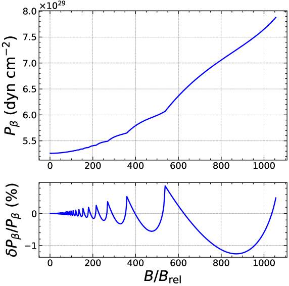
Figure 11: Top panel: Exact threshold pressure (in cgs units) for the onset of electron captures by ¹²²Zr as a function of the magnetic field strength $B_{\star}=B/B_{\rm rel}$ up to the onset of the strongly quantizing regime. Bottom panel: Relative error (in %) of the approximate analytical expression.

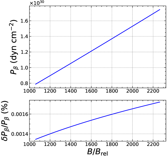
Figure 12: Same as Figure 11 in the strongly quantizing regime.

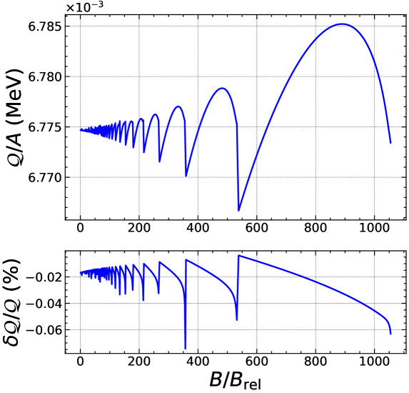
Figure 13: Top panel: Exact heat released per nucleon from electron captures by ¹²²Zr as a function of the magnetic field strength $B_{\star}=B/B_{\rm rel}$ up to the onset of the strongly quantizing regime. Bottom panel: Relative error (in %) of the approximate analytical expression.

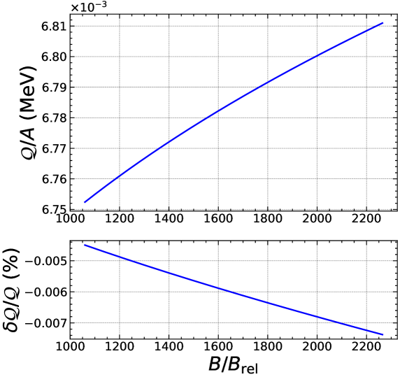
Figure 14: Same as Figure 13 in the strongly quantizing regime.

6 Conclusions

We have derived accurate analytical formulas (with typical errors below 1%) for calculating the threshold density $\bar{n}_{\beta}$ and pressure $P_{\beta}$ for the onset of electron captures by nuclei in the shallow layers of magnetar crusts, as well as the maximum amount of heat released $\mathcal{Q}$ taking into account the Landau–Rabi quantization of electron motion induced by the magnetic field. We have also obtained formulas for determining the initial constitution of the outer crust. These formulas are applicable over the whole range of magnetic fields encountered in neutron stars, from the weakly quantizing regime to the most extreme situation in which the electrons all lie in the lowest Landau–Rabi level.

Using experimental nuclear data supplemented with predictions from the atomic mass model HFB-24, we have calculated all the necessary nuclear parameters to calculate the shallow heating for any given magnetic field considering both ground-state to ground-state and ground-state to excited-state transitions. Full numerical results can be found in Chamel and Fantina (2022). Together with the results for the equation of state and superfluid properties published in Mutafchieva et al. (2019); Pearson et al. (2018, 2020); Pearson and Chamel (2022); Allard and Chamel (2021), they provide consistent microscopic inputs for modelling the magneto-thermal evolution of neutron stars.

Conceptualization, N.C.; methodology, N.C.; software, N.C. and A.F.F.; validation, N.C. and A.F.F.; formal analysis, N.C.; investigation, N.C.; writing—original draft preparation, N.C.; writing—review and editing, N.C. and A.F.F.; visualization, N.C.; supervision, N.C.; project administration, N.C. All authors have read and agreed to the published version of the manuscript.

The work of N.C. was funded by Fonds de la Recherche Scientifique-FNRS (Belgium) under Grant Number IISN 4.4502.19. This work was also partially supported by the European Cooperation in Science and Technology Action CA16214 and the CNRS International Research Project (IRP) “Origine des éléments lourds dans l’univers: Astres Compacts et Nucléosynthèse (ACNu)”.

Not applicable.

Not applicable.

The data analyzed in this paper can be found in the 2016 Atomic Mass Evaluation Wang et al. (2017), the BRUSLIB database (http://www.astro.ulb.ac.be/bruslib/, accessed on 9 June 2022, see Xu et al. (2013)), and the Nuclear Data section of the International Atomic Energy Agency website (https://www-nds.iaea.org/relnsd/NdsEnsdf/QueryForm.html, accessed on 9 June 2022). The results presented in this study are openly available on the Zenodo repository Chamel and Fantina (2022).

The authors declare no conflict of interest.

References

References

• Esposito et al. (2021) Esposito, P.; Rea, N.; Israel, G.L. Magnetars: A Short Review and Some Sparse Considerations. In Astrophysics and Space Science Library; Belloni, T.M., Méndez, M., Zhang, C., Eds.; Springer: Berlin/Heidelberg, Germany, 2021; Volume 461, pp. 97–142. https://doi.org/10.1007/978-3-662-62110-3_3.
• Duncan and Thompson (1992) Duncan, R.C.; Thompson, C. Formation of Very Strongly Magnetized Neutron Stars: Implications for Gamma-Ray Bursts. Astrophys. J. Lett. 1992, 392, L9. https://doi.org/10.1086/186413.
• Olausen and Kaspi (2014) Olausen, S.A.; Kaspi, V.M. The McGill Magnetar Catalog. Astrophys. J. Suppl. 2014, 212, 6. https://doi.org/10.1088/0067-0049/212/1/6.
• Viganò et al. (2013) Viganò, D.; Rea, N.; Pons, J.A.; Perna, R.; Aguilera, D.N.; Miralles, J.A. Unifying the observational diversity of isolated neutron stars via magneto-thermal evolution models. Mon. Not. R. Astron. Soc. 2013, 434, 123–141. https://doi.org/10.1093/mnras/stt1008.
• Beloborodov and Li (2016) Beloborodov, A.M.; Li, X. Magnetar Heating. Astrophys. J. 2016, 833, 261. https://doi.org/10.3847/1538-4357/833/2/261.
• De Grandis et al. (2020) De Grandis, D.; Turolla, R.; Wood, T.S.; Zane, S.; Taverna, R.; Gourgouliatos, K.N. Three-dimensional Modeling of the Magnetothermal Evolution of Neutron Stars: Method and Test Cases. Astrophys. J. 2020, 903, 40. https://doi.org/10.3847/1538-4357/abb6f9.
• Fantina et al. (2020) Fantina, A.F.; De Ridder, S.; Chamel, N.; Gulminelli, F. Crystallization of the outer crust of a non-accreting neutron star. Astron. Astrophys. 2020, 633, A149. https://doi.org/10.1051/0004-6361/201936359.
• Carreau et al. (2020) Carreau, T.; Gulminelli, F.; Chamel, N.; Fantina, A.F.; Pearson, J.M. Crystallization of the inner crust of a neutron star and the influence of shell effects. Astron. Astrophys. 2020, 635, A84. https://doi.org/10.1051/0004-6361/201937236.
• Kaminker et al. (2006) Kaminker, A.D.; Yakovlev, D.G.; Potekhin, A.Y.; Shibazaki, N.; Shternin, P.S.; Gnedin, O.Y. Magnetars as cooling neutron stars with internal heating. Mon. Not. R. Astron. Soc. 2006, 371, 477–483. https://doi.org/10.1111/j.1365-2966.2006.10680.x.
• Kaminker et al. (2009) Kaminker, A.D.; Potekhin, A.Y.; Yakovlev, D.G.; Chabrier, G. Heating and cooling of magnetars with accreted envelopes. Mon. Not. R. Astron. Soc. 2009, 395, 2257–2267. https://doi.org/10.1111/j.1365-2966.2009.14693.x.
• Cooper and Kaplan (2010) Cooper, R.L.; Kaplan, D.L. Magnetic Field-Decay-Induced Electron Captures: A Strong Heat Source in Magnetar Crusts. Astrophys. J. Lett. 2010, 708, L80–L83. https://doi.org/10.1088/2041-8205/708/2/L80.
• Haensel and Zdunik (1990) Haensel, P.; Zdunik, J.L. Non-equilibrium processes in the crust of an accreting neutron star. Astron. Astrophys. 1990, 227, 431–436.
• Chamel et al. (2021) Chamel, N.; Fantina, A.F.; Suleiman, L.; Zdunik, J.L.; Haensel, P. Heating in Magnetar Crusts from Electron Captures. Universe 2021, 7, 193. https://doi.org/10.3390/universe7060193.
• Goriely et al. (2013) Goriely, S.; Chamel, N.; Pearson, J.M. Further explorations of Skyrme-Hartree-Fock-Bogoliubov mass formulas. XIII. The 2012 atomic mass evaluation and the symmetry coefficient. Phys. Rev. C 2013, 88, 024308. https://doi.org/10.1103/PhysRevC.88.024308.
• Pearson et al. (2018) Pearson, J.M.; Chamel, N.; Potekhin, A.Y.; Fantina, A.F.; Ducoin, C.; Dutta, A.K.; Goriely, S. Unified equations of state for cold non-accreting neutron stars with Brussels-Montreal functionals—I. Role of symmetry energy. Mon. Not. R. Astron. Soc. 2018, 481, 2994–3026. https://doi.org/10.1093/mnras/sty2413.
• Pearson et al. (2020) Pearson, J.M.; Chamel, N.; Potekhin, A.Y. Unified equations of state for cold nonaccreting neutron stars with Brussels-Montreal functionals. II. Pasta phases in semiclassical approximation. Phys. Rev. C 2020, 101, 015802. https://doi.org/10.1103/PhysRevC.101.015802.
• Pearson and Chamel (2022) Pearson, J.M.; Chamel, N. Unified equations of state for cold nonaccreting neutron stars with Brussels-Montreal functionals. III. Inclusion of microscopic corrections to pasta phases. Phys. Rev. C 2022, 105, 015803. https://doi.org/10.1103/PhysRevC.105.015803.
• Mutafchieva et al. (2019) Mutafchieva, Y.D.; Chamel, N.; Stoyanov, Z.K.; Pearson, J.M.; Mihailov, L.M. Role of Landau-Rabi quantization of electron motion on the crust of magnetars within the nuclear energy density functional theory. Phys. Rev. C 2019, 99, 055805. https://doi.org/10.1103/PhysRevC.99.055805.
• Rabi (1928) Rabi, I.I. Das freie Elektron im homogenen Magnetfeld nach der Diracschen Theorie. Z. Fur. Phys. 1928, 49, 507–511. https://doi.org/10.1007/BF01333634.
• Landau (1930) Landau, L. Diamagnetismus der Metalle. Z. Fur Phys. 1930, 64, 629–637. https://doi.org/10.1007/BF01397213.
• Tiengo et al. (2013) Tiengo, A.; Esposito, P.; Mereghetti, S.; Turolla, R.; Nobili, L.; Gastaldello, F.; Götz, D.; Israel, G.L.; Rea, N.; Stella, L.; et al. A variable absorption feature in the X-ray spectrum of a magnetar. Nature 2013, 500, 312–314. https://doi.org/10.1038/nature12386.
• An et al. (2014) An, H.; Kaspi, V.M.; Beloborodov, A.M.; Kouveliotou, C.; Archibald, R.F.; Boggs, S.E.; Christensen, F.E.; Craig, W.W.; Gotthelf, E.V.; Grefenstette, B.W.; et al. NuSTAR Observations of X-Ray Bursts from the Magnetar 1E 1048.1-5937. Astrophys. J. 2014, 790, 60. https://doi.org/10.1088/0004-637X/790/1/60.
• Uryū et al. (2019) Uryū, K.; Yoshida, S.; Gourgoulhon, E.; Markakis, C.; Fujisawa, K.; Tsokaros, A.; Taniguchi, K.; Eriguchi, Y. New code for equilibriums and quasiequilibrium initial data of compact objects. IV. Rotating relativistic stars with mixed poloidal and toroidal magnetic fields. Phys. Rev. D 2019, 100, 123019. https://doi.org/10.1103/PhysRevD.100.123019.
• Chamel et al. (2015) Chamel, N.; Fantina, A.F.; Zdunik, J.L.; Haensel, P. Neutron drip transition in accreting and nonaccreting neutron star crusts. Phys. Rev. C 2015, 91, 055803. https://doi.org/10.1103/PhysRevC.91.055803.
• Haensel et al. (2007) Haensel, P.; Potekhin, A.Y.; Yakovlev, D.G. Neutron Stars. 1. Equation of State and Structure; Springer: New York, NY, USA, 2007.
• Van Vleck (1932) Van Vleck, J.H. The Theory of Electric and Magnetic Susceptibilities; Oxford University Press: London, UK, 1932.
• Baiko (2009) Baiko, D.A. Coulomb crystals in the magnetic field. Phys. Rev. E 2009, 80, 046405. https://doi.org/10.1103/PhysRevE.80.046405.
• Baiko et al. (2001) Baiko, D.A.; Potekhin, A.Y.; Yakovlev, D.G. Thermodynamic functions of harmonic Coulomb crystals. Phys. Rev. E 2001, 64, 057402. https://doi.org/10.1103/PhysRevE.64.057402.
• Potekhin and Chabrier (2013) Potekhin, A.Y.; Chabrier, G. Equation of state for magnetized Coulomb plasmas. Astron. Astrophys. 2013, 550, A43. https://doi.org/10.1051/0004-6361/201220082.
• Salpeter (1954) Salpeter, E.E. Electrons Screening and Thermonuclear Reactions. Aust. J. Phys. 1954, 7, 373. https://doi.org/10.1071/PH540373.
• Dib and Espinosa (2001) Dib, C.O.; Espinosa, O. The magnetized electron gas in terms of Hurwitz zeta functions. Nucl. Phys. B 2001, 612, 492–518. https://doi.org/10.1016/S0550-3213(01)00360-1.
• Chamel and Fantina (2015) Chamel, N.; Fantina, A.F. Electron capture instability in magnetic and nonmagnetic white dwarfs. Phys. Rev. D 2015, 92, 023008. https://doi.org/10.1103/PhysRevD.92.023008.
• Chamel (2020) Chamel, N. Analytical determination of the structure of the outer crust of a cold nonaccreted neutron star. Phys. Rev. C 2020, 101, 032801. https://doi.org/10.1103/PhysRevC.101.032801.
• Chamel and Stoyanov (2020) Chamel, N.; Stoyanov, Zh.K. Analytical determination of the structure of the outer crust of a cold nonaccreted neutron star: Extension to strongly quantizing magnetic fields. Phys. Rev. C 2020, 101, 065802. https://doi.org/10.1103/PhysRevC.101.065802.
• Chamel (2020) Chamel, N. Equilibrium Structure of the Outer Crust of a Cold Nonaccreted Neutron Star; Zenodo: Geneva, Switzerland, 2020. https://doi.org/10.5281/zenodo.3719439.
• Chamel and Stoyanov (2020) Chamel, N.; Stoyanov, Zh. Equilibrium Structure of the Outer Crust of a Magnetar; Zenodo: Geneva, Switzerland, 2020. https://doi.org/10.5281/zenodo.3839787.
• Pons and Viganò (2019) Pons, J.A.; Viganò, D. Magnetic, thermal and rotational evolution of isolated neutron stars. Living Rev. Comput. Astrophys. 2019, 5, 3. https://doi.org/10.1007/s41115-019-0006-7.
• Chamel and Fantina (2016) Chamel, N.; Fantina, A.F. Binary and ternary ionic compounds in the outer crust of a cold nonaccreting neutron star. Phys. Rev. C 2016, 94, 065802. https://doi.org/10.1103/PhysRevC.94.065802.
• Peña Arteaga et al. (2011) Peña Arteaga, D.; Grasso, M.; Khan, E.; Ring, P. Nuclear structure in strong magnetic fields: Nuclei in the crust of a magnetar. Phys. Rev. C 2011, 84, 045806. https://doi.org/10.1103/PhysRevC.84.045806.
• Fantina et al. (2016) Fantina, A.F.; Chamel, N.; Mutafchieva, Y.D.; Stoyanov, Zh.K.; Mihailov, L.M.; Pavlov, R.L. Role of the symmetry energy on the neutron-drip transition in accreting and nonaccreting neutron stars. Phys. Rev. C 2016, 93, 015801. https://doi.org/10.1103/PhysRevC.93.015801.
• Wang et al. (2017) Wang, M.; Audi, G.; Kondev, F.G.; Huang, W.J.; Naimi, S.; Xu, X. The AME2016 atomic mass evaluation (II). Tables, graphs and references. Chin. Phys. C 2017, 41, 030003. https://doi.org/10.1088/1674-1137/41/3/030003.
• Xu et al. (2013) Xu, Y.; Goriely, S.; Jorissen, A.; Chen, G.L.; Arnould, M. Databases and tools for nuclear astrophysics applications. BRUSsels Nuclear LIBrary (BRUSLIB), Nuclear Astrophysics Compilation of REactions II (NACRE II) and Nuclear NETwork GENerator (NETGEN). Astron. Astrophys. 2013, 549, A106. https://doi.org/10.1051/0004-6361/201220537.
• Allard and Chamel (2021) Allard, V.; Chamel, N. 1S0 Pairing Gaps, Chemical Potentials and Entrainment Matrix in Superfluid Neutron-Star Cores for the Brussels-Montreal Functionals. Universe 2021, 7, 470. https://doi.org/10.3390/universe7120470.
• Perot et al. (2019) Perot, L.; Chamel, N.; Sourie, A. Role of the symmetry energy and the neutron-matter stiffness on the tidal deformability of a neutron star with unified equations of state. Phys. Rev. C 2019, 100, 035801. https://doi.org/10.1103/PhysRevC.100.035801.
• Chamel and Fantina (2022) Chamel, N.; Fantina, A.F. Onset of Electron Captures and Shallow Heating in Magnetars [Data Set]; Zenodo: Geneva, Switzerland, 2022. https://doi.org/10.5281/zenodo.6604639.