Data-Efficient Learning via Minimizing Hyperspherical Energy

Abstract

Deep learning on large-scale data is dominant nowadays. The unprecedented scale of data has been arguably one of the most important driving forces for the success of deep learning. However, there still exist scenarios where collecting data or labels could be extremely expensive, e.g., medical imaging and robotics. To fill up this gap, this paper considers the problem of data-efficient learning from scratch using a small amount of representative data. First, we characterize this problem by active learning on homeomorphic tubes of spherical manifolds. This naturally generates feasible hypothesis class. With homologous topological properties, we identify an important connection – finding tube manifolds is equivalent to minimizing hyperspherical energy (MHE) in physical geometry. Inspired by this connection, we propose a MHE-based active learning (MHEAL) algorithm, and provide comprehensive theoretical guarantees for MHEAL, covering convergence and generalization analysis. Finally, we demonstrate the empirical performance of MHEAL in a wide range of applications on data-efficient learning, including deep clustering, distribution matching, version space sampling and deep active learning.

1 Introduction

Recent years have witnessed the success of deep learning [1] in a wide range of applications in computer vision [2], natural language processing [3], and speech processing [4]. The fuel that drives the progress made by deep learning is the unprecedented scale of available datasets [5, 6]. Taking advantage of a huge amount of data and annotations, some powerful artificial intelligence (AI) systems are built, e.g., Deep Blue [7], AlphaGo [8], etc. Despite their superior performance, training and annotating large-scale data are quite expensive. In contrast, humans can easily learn to distinguish a dog and a wolf by glancing one picture. This motivates us to study the scenario where only a small amount of data is available for AI systems.

There are several related techniques that study how to learn efficiently from a small amount of data or annotations, such as few-shot learning [9], active learning [10], and unsupervised representation learning [11]. Besides, data augmentation [12] and generative models [13] can also be used to help data-efficient learning. This leads to a broad interest for our study. To narrow our scope, we focus on the generalization performance of a small amount of efficient data distributed over the version space. Given a finite hypothesis class, data distributed around the decision boundary of version space usually generate effective hypotheses, and also produce significant updates for the model. We thus adopt a novel perspective for data-efficient learning – characterizing data representation via the topology of decision boundary.

Figure 1: Active learning shrinks the version space $\mathcal{V}$ into its optimal expression $\mathcal{V}^{*}$ which tightly covers the decision boundaries of the two spherical classes, deriving effective hypotheses. There are a small amount of data distributed around the decision boundaries, which characterize their topological structures.

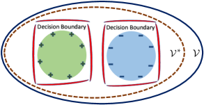
Active learning (AL), which initializes with any hypothesis (even a null hypothesis), is a promising tool to learn the topology of decision boundary via iteratively shrinking the version space (see Figure 1). Specifically, the highly informative data which derive the hypothesis updates are distributed in version space regions (called in-version-space), which maintain homeomorphic manifolds [14] over the topological properties of decision boundaries. Hereafter, an AL algorithm that uses in-version-space sampling is termed version space-based AL (VSAL) [15]. Usually, a typical sampling criterion of VSAL is to select those data which disagree with the current hypothesis the most, where error disagreement [16] is one effective indicator to control the sample selection.

To identify a small amount of efficient data, typical VSAL algorithms estimate the error disagreements by repeatedly visiting the topology of decision boundaries. This strategy leads to one major drawback of computational intractability [17]. Moreover, computational estimations/approximations on generalization error may mislead the data selection, resulting in incorrect or biased sampling. The reason behind lies in two folds: 1) poor initialization of model parameters, and 2) incremental estimations/approximations. This motivates us to learn from a small amount of data without error estimation. Instead, we propose to utilize the topological properties of the version space for data-efficient learning.

Figure 2: MHE on a sphere with a radius $r$. Left to right: $N=\{2,3,5\}$, where $N$ denotes the number of the electrons. Red points denote electrons. Dash lines denote the level of potential energy. MHE performs small yet effective data sampling from decision boundaries of version space.

Figure 3: Pipeline of MHEAL. Input distribution is clustered into a set of spheres which perform MHE. MHE then characterizes decision boundaries of each cluster by a small amount of representative data points (labeled in red).

In physical geometry, there is a parallel problem, namely minimizing hyperspherical energy (MHE) [18] for $N$ electrons (see Figure 2), which preserves homologous topological properties over a spherical version space. The standard MHE includes its $\ell_{0}$, $\ell_{1}$, and $\ell_{2}$ expressions using a natural generalization of the 0,1,2-norm for finite-dimensional vector spaces, respectively. Geometrically, MHE is equivalent to characterizing decision boundaries of a version space via homeomorphic tube manifold [19], which naturally generates feasible hypothesis class. This paper aims at learning with a small amount of data from decision boundaries via the proposed MHE-based AL (MHEAL) algorithm. To characterize these representative data, we maximize the lower bound of the optimal $\ell_{0}$ expression of MHE as a feasible and efficient approximation over each pre-estimated spherical cluster (see Figure 3). Our theoretical insights show that this approximation enjoys the properties of geometric preservation and controllable approximation accuracy. In the importance weighting setting of AL, we further prove that MHEAL yields a faster hypothesis-pruning speed, which then leads to tighter bounds on its generalization error and label complexity. A high-level summarization of this paper is given as follows:

• Goal: Learning efficient-representative data from homeomorphic tubes of spherical manifolds via AL.

• Motivation: Exploring data representation from decision boundary by typical VSAL has computational intractability. To address this, we characterize the topological properties of version space by MHE.

• Solution: We propose the MHEAL algorithm with theoretical guarantees on generalization error and label complexity.

Our major contributions are summarized as follows:

• We study data-efficient learning as an important step toward training AI systems with a small amount of data. In a nutshell, we propose to characterize the decision boundaries of version space by minimizing the hyperspherical energy of a small amount of representative data.

• We derive a lower bound maximization scheme to approximate the greedy sequential solution of $\ell_{0}$ expression of MHE, yielding a much lower computation complexity.

• We give theoretical analyses for our approximation optimization scheme which guarantees both geometric preservation and approximation accuracy.

• We propose a novel active learning algorithm called MHEAL, which performs MHE over each pre-estimated spherical cluster in an unsupervised manner and effectively characterizes their decision boundaries.

• We prove the theoretical convergence of MHEAL by deriving its generalization error and label complexity bounds. Moreover, we conduct an extensive empirical study on the generalization performance to demonstrate the effectiveness of our bounds.

2 Related Work

VSAL presents a theoretical interpretation for learning from representative data via AL, and MHE implements an advanced VSAL algorithm from physical geometry. We briefly introduce related work from these two aspects.

VSAL The VSAL algorithm [15, 17] prunes the hypothesis class by annotating the unlabeled data via the hypothesis disagreement maximization, which requires the optimal hypothesis always to be included. Specifically, the hypothesis-pruning [20] always needs to maintain a correct update, where error disagreement [21] is an important indicator to control these updates. With the estimation on errors, the error disagreement indicator can be specified as the best-in-class error [22], average-in-class error [23], entropy of error [24], etc. A series of confidence label complexity bounds were derived under noise-free settings, such as the agnostic PAC bound [25, 26, 27, 28]. With a desired error threshold, the annotating budget is also bounded. By employing importance weighting, importance weighted AL (IWAL) [29] utilizes the on-line sampling theory to tighten the label complexity bounds, before converging into the optimal hypothesis. To further improve it, [23] gives more refined analysis on the current hypothesis class to reduce the best-in-class error, resulting in a tighter bound on label complexity [16]. Guarantees under different noise settings are also studied, e.g., adversarial noise [30], malicious noise [31], random classification noise [32], and bounded noise [33].

Few-shot learning [9] also studies how to adapt to a new task with a very small amount of data, but it typically requires extra information about the base tasks. Moreover, few-shot learning mostly considers the passive setting where the label distribution is explicitly controlled by one specific sampling scenario in the pre-defined training set. In contrast, AL that learns from scratch using representative data is not as limited as few-shot learning, since its algorithms can stop their iterative sampling either when they achieve desired accuracy or when the annotation budgets are exhausted.

MHE Thomson problem [34] in physics describes the ground state energy and configuration of a set of electrons on a unit hypersphere. Given $N$ electrons, Liu et al. [18] seek to achieve their minimum potential energy by considering their interactions on a unit hypersphere. This also can be viewed as maximizing hyperspherical uniformity [35]. Recent studies [36, 37, 38, 39] have shown that hyperspherical similarity preserves the most abundant and discriminative information. Modeling with DNNs, geodesic distances [40] between neurons that discriminate the features, are projected and optimized on the hypersphere. However, naively minimizing hyperspherical energy from geometry suffers from some difficulties due to the underlying non-linearity and non-convexity. To alleviate these difficulties, Lin et al. [41] propose the compressive MHE (CoMHE) as a more effective regularization to minimize hyperspherical energy for neural networks. Following [18, 41], Perez-Lapillo et al. [42] and Shah et al. [43] improve voice separation by applying MHE to Wave-U-Net and time-frequency domain networks, respectively. MHE has wide applications in image recognition [39, 44, 45], face recognition [36, 18, 46], speaker verification [47], adversarial robustness [48], few-shot learning [49, 50], etc.

Figure 4: Characterization of a 2D decision boundary by a tube manifold $\mathcal{M}$ with a width $\gamma$.

3 MHE and Decision Boundary

Section 3.1 characterizes the homologous topological properties of decision boundaries for tube manifolds. Section 3.2 presents the MHE problem of physical geometry. Section 3.3 then proposes a sequential solution for $\ell_{0}$ expression of MHE. To find an alternative scheme for such a greedy solution, Section 3.4 maximizes the lower bound of the optimal $\ell_{0}$ expression of MHE as a feasible approximation.

3.1 Decision Boundary

We start by characterizing the decision boundaries. Given a feature space $\mathcal{X}$ associating with a label space $\mathcal{Y}$, let $\mathcal{Y}=\{1,2,...,K\}$, we define $P_{\mathcal{X}\mathcal{Y}}$ as the joint distribution over the mapping from $\mathcal{X}$ to $\mathcal{Y}$. According to the Bayesian theorem, decision boundary of a class (cluster) can be constructed on a tube manifold $\mathcal{M}$ [14]. We next give a conceptual description for decision boundaries in the multi-class setting.

Definition 1 (Decision boundary).

Given a class i.i.d. drawn from $P_{\mathcal{X}\mathcal{Y}}$ with label $k$ embedded in a label space $\mathcal{Y}\in\{1,2,3,...,K\}$, $k^{\prime}\in\mathcal{Y}$ and $k^{\prime}\neq k$, the decision boundary of this class is distributed over a tube manifold $\mathcal{M}$ with uncertain label predictions, which satisfy $\mathcal{M}:=\{x\in\mathcal{X}|P_{\mathcal{Y}|\mathcal{X}}(k^{\prime}|x)=P_{\mathcal{Y}|\mathcal{X}}(k|x)\}$, where the optimal Bayesian classifier is $f(x)=k$ if $P_{\mathcal{Y}|\mathcal{X}}(k|x)\geq 0.5$, otherwise $f(x)=k^{\prime}\in\{1,2,...,k-1,k+1,...,K\}$.

Remark 1.

Definition 1 characterizes the decision boundary of a tube manifold over a label space $\mathcal{Y}$, where those samples around the tube are with uncertain class labels. For any high-dimensional sphere, the tube manifold still covers those samples with uncertain labels distributed near the boundary of the class.

If $\mathcal{Y}$ is a binary label space, that is, $\mathcal{Y}\in\{+1,-1\}$, we then adapt Definition 1 into the following specific case.

Example 1 (Binary case of decision boundary).

Given a class embedded in a label space $\mathcal{Y}=\{+1,-1\}$, its decision boundary is distributed over a tube manifold $\mathcal{M}$ with uncertain label predictions, which satisfy $\mathcal{M}:=\{x\in\mathcal{X}|P_{\mathcal{Y}|\mathcal{X}}(+1|x)=P_{\mathcal{Y}|\mathcal{X}}(-1|x)\}$, where the optimal Bayesian classifier is $f(x)=+1$ if $P_{\mathcal{Y}|\mathcal{X}}(+1|x)\geq 0.5$, otherwise $f(x)=-1$.

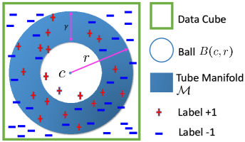
From a geometric perspective [19], the manifold of decision boundary can be characterized by a tube with a width $\gamma$, which keeps homologous properties with a ball $B(c,r)$, where $c$ denotes the center and $r$ denotes the radius (see Figure 4). We give the following assumption for the homeomorphic tube manifold, where $B(c,r-\gamma)$ denotes the concentric ball of $B(c,r)$. Specifically, $r-\gamma$ is the radius, $c$ is the center, and $\gamma$ is a variable to denote the width of the tube manifold.

Assumption 1.

Assume that the label complexity of a version space-based hypothesis is characterized by a set $S$ over the tube manifold $\mathcal{M}:=\{B(c,r)\backslash B(c,r-\gamma)\}$, if $S\subseteq D^{1}=\{x\in\mathcal{X}:f(x)=+1\}$, we have: 1) $\bigcap_{x_{i}\in S}\mathcal{M}(x_{i},\gamma)\neq\emptyset$, where $\mathcal{M}(x_{i},\gamma)$ denotes the tube manifold covering $x_{i}$ with a width $\gamma$; 2) let $D^{-1}=\{x\in\mathcal{X}:f(x)=-1\}$, if $x_{i}\subseteq D^{+1}$ and $x_{j}\subseteq D^{-1}$, there exists $\|x_{i}-x_{j}\|\leq\gamma$, where $\|\cdot\|$ denotes the $\ell_{2}$-norm.

In Assumption 1, the first condition requires that there is a homeomorphic tube of $\mathcal{M}$ with a width $\gamma$ which covers $x_{i}\in S$ to contain shared elements from both classes. This means that $\mathcal{M}$ is a tight covering for $S$. The second condition describes the width of $\mathcal{M}$, i.e., $\gamma$. We have defined decision boundaries to characterize those feasible hypothesis class as a consistent concept, and then generalize it with MHE.

3.2 MHE

MHE [18] seeks to find the configuration of $N$ mutually-repelling electrons that minimizes the potential energy. These electrons are distributed on a unit hypersphere. In physics, such a potential energy is used to describe a balanced state of the distribution of electrons. More generally, MHE corresponds to the uniform distribution on the hypersphere [35]. From a geometric perspective, it can be used to characterize the decision boundary distributed in a homeomorphic tube manifold of a hypersphere.

Given $N$ samples, i.e., $\mathcal{W}=\{w_{1},w_{2},...,w_{N}\in\mathbb{R}^{d}\}$, let $\hat{w}_{i}$ denote the $\ell_{2}$-norm projection of $w_{i}$ on the unit hypersphere. Then their hyperspherical energy can be defined as

$$\begin{split}\mathbb{E}_{s,d}(\hat{w}_{i}|_{i=1}^{N}):&=\sum_{i=1}^{N}\sum_{j=1}^{N}f_{s}(\|\hat{w}_{i}-\hat{w}_{j}\|)\\ &=\left\{\begin{array}[]{lr}\sum_{i>j}\|\hat{w}_{i}-\hat{w}_{j}\|^{-s},&s>0\\ \sum_{i>j}{\rm log}(\|\hat{w}_{i}-\hat{w}_{j}\|^{-1}),&s=0\\ \end{array}\right.,\end{split}$$ (1)

where $f_{s}$ denotes an energy function, and $i,j\geq 1$. Specifically, $\mathbb{E}_{0,d}$ denotes the logarithmic potential energy, that is, the $\ell_{0}$ expression of MHE (also termed as $\ell_{0}$ MHE), i.e., $\mathbb{E}_{0,d}=\sum_{i>j}{\rm log}(\|\hat{w}_{i}-\hat{w}_{j}\|^{-1})$. Then, minimizing the $\ell_{0}$ hyperspherical energy can be viewed as an approximation to minimizing $\mathbb{E}_{s,d}$ [18]. $\ell_{0}$ MHE is formally defined as

$$\begin{split}\operatorname*{arg\,min}_{w_{1},w_{2},...,w_{N}}\mathbb{E}_{0,d}&=\sum_{i>j}{\rm log}(\|\hat{w}_{i}-\hat{w}_{j}\|^{-1})\\ &=\operatorname*{arg\,max}_{w_{1},w_{2},...,w_{N}}\prod_{i>j}\|\hat{w}_{i}-\hat{w}_{j}\|.\end{split}$$ (2)

Eq. (2) is essentially a limiting case of the MHE objective $\mathbb{E}_{s,d}$ [18]. Besides this, $\mathbb{E}_{1,d}$ and $\mathbb{E}_{2,d}$ are also feasible alternatives, namely $\ell_{1}$ and $\ell_{2}$ expressions of MHE, respectively (also term $\ell_{1}$ MHE and $\ell_{2}$ MHE). However, minimizing $\mathbb{E}_{1,d}$ is a typical NP hard problem, which usually requires a sequential search. $\mathbb{E}_{2,d}$ can be solved by gradient descent with the following gradient [41]:

$$\begin{split}\nabla_{\hat{w}_{i}}\mathbb{E}_{2,d}=\sum_{j=1,j\neq i}\frac{-2(\hat{w}_{i}-\hat{w}_{j})}{\|\hat{w}_{i}-\hat{w}_{j}\|^{4}},\end{split}$$ (3)

whose solution yields $\hat{w}_{i}=\frac{\sum_{j=1}^{N}\|\hat{w}_{i}-\hat{w}_{j}\|^{-4}\hat{w}_{j}}{\sum_{j=1}^{N}\|\hat{w}_{i}-\hat{w}_{j}\|^{-4}}$ s.t. $j\neq i$.

3.3 Sequential Optimization of MHE

We here present the optimal solution of $\ell_{0}$ MHE by employing a greedy strategy. Given $\mathcal{P}$ containing $M$ feasible data points in $\mathbb{R}^{d}$, MHE is performed to find $N$ data points for $\mathcal{W}$. Let $\hat{w}_{1}\in{P}$ and $\mathcal{W}$ be initialized by $\mathcal{W}=\{\hat{w}_{1}\}$. At the $t$-th step, a sequential optimization is adopted to find $\hat{w}_{t}$ from $\mathcal{P}$

$$\begin{split}\hat{w}_{t}&=\operatorname*{arg\,max}_{{\hat{p}}\in\mathcal{P}}\prod_{u,v\in\{{\hat{w}_{1}},\cdots,{\hat{w}_{t-1}},{\hat{p}}\}}\|u-v\|\\ &=\operatorname*{arg\,max}_{{\hat{p}}\in\mathcal{P}}\prod_{t-1\geq i\geq 1}\|\hat{w}_{i}-\hat{p}\|,\end{split}$$ (4)

after which $\mathcal{W}$ is updated by adding a new data point, i.e., $\mathcal{W}\leftarrow\mathcal{W}\cup\{\hat{w}_{t}\}$ at the $t$-th step. In this setting, computing one sample costs $\mathcal{O}(MN)$ complexity, where the argmax operation costs $\mathcal{O}(M)$, and the computation of $\prod_{t-1\geq i>1}$ costs $\mathcal{O}(N)$. To obtain $N$ feasible samples, Eq. (4) is computed until $t$ arrives at $N$, thereby costing $\mathcal{O}(MN^{2})$.

Let $\mathcal{L}_{\mathbb{E}_{0,d}}({\hat{w}}_{1})$ denote the $\ell_{0}$ hyperspherical energy of $N$ data points with an initial sample ${\hat{w}}_{1}$, the optimal initialization on ${\hat{w}}_{1}$, i.e., ${\hat{w}}_{1}^{*}$, is obtained by

$$\begin{split}{\hat{w}}_{1}^{*}=\operatorname*{arg\,max}_{\hat{p}\in\mathcal{P}}\mathcal{L}_{\mathbb{E}_{0,d}}(\hat{p}).\end{split}$$ (5)

For $M$ times of the sequential optimization in Eq. (5), it will cost $\mathcal{O}(M^{2}N^{2})$ to obtain the optimal ${\hat{w}}_{1}$. A detailed process is then presented in Algorithm 1.

1 Input: $\mathcal{P}=\{\hat{p}_{1},\hat{p}_{2},...,\hat{p}_{M}\}$ containing $M$ feasible data points in $\mathbb{R}^{d}$.

2 Initialize: $l=0$.

3 while $l<M$ do

4       $\hat{w}_{1}=\hat{p}_{l}$, $\mathcal{W}=\{{\hat{w}}_{1}\}$.

5       for $t=2,...,N$ do

6             $\hat{w}_{t}=\operatorname*{arg\,max}_{{\hat{p}}\in\mathcal{P}}\prod_{t-1\geq i\geq 1}\|\hat{w}_{i}-\hat{p}\|$

7             $\mathcal{W}\leftarrow\mathcal{W}\cup\{\hat{w}_{t}\}$

8       end for

9      Obtain the energy: $\mathcal{L}_{\mathbb{E}_{0,d}}(\hat{p}_{l})=\prod_{\mathcal{W},i>j}\|\hat{w}_{i}-\hat{w}_{j}\|.$

10      

11 end while

Output: The optimal ${\hat{w}}_{1}^{*}$ from $\operatorname*{arg\,max}_{\hat{p}_{l}\in\mathcal{P}}\mathcal{L}_{\mathbb{E}_{0,d}}(\hat{p}_{l}),$ and its optimal energy expression $\mathcal{L}_{\mathbb{E}_{0,d}}({\hat{w}}_{1}^{*})$.

Algorithm 1 Sequential optimization of $\ell_{0}$ MHE

3.4 Approximation by Lower Bound Maximization

The sequential optimization comes with a computation complexity of $\mathcal{O}(M^{2}N^{2})$, which is not efficient to solve. We thus aim to find a feasible approximation.

Proposition 1.

Assume that $\hat{w}_{1},\hat{w}_{2},...,\hat{w}_{N-1}$ are known samples for $\mathcal{W}$, the following step is to optimize $\hat{w}_{N}$, that is, $\hat{w}_{N}=\operatorname*{arg\,max}_{\hat{p}\in\mathcal{P}}\mathcal{L}_{\mathbb{E}_{0,d}}(\hat{p}),$ $s.t.\ \mathcal{W}=\{\hat{w}_{1},\hat{w}_{2},...,\hat{w}_{N-1}\}$, where this argmax operation invokes Eq. (4) one time since $\mathcal{W}$ has already included $N-1$ samples. With such setting, assume that $\min_{\hat{w}_{j}\in\mathcal{W}}\|\hat{w}_{N}-\hat{w}_{j}\|\leq\min_{\hat{w}_{i},\hat{w}_{j}\in\mathcal{W}}\|\hat{w}_{i}-\hat{w}_{j}\|$, recalling the energy definition of Eq. (2), there exists an inequality

$$\begin{split}&\Big{(}\min_{\hat{w}_{j}\in\mathcal{W}}\|\hat{w}_{N}-\hat{w}_{j}\|\Big{)}^{{\frac{N^{2}-N}{2}}}\leq\\ &\Big{(}\!\prod_{N-1>i>j}\!\|\hat{w}_{i}-\hat{w}_{j}\|\Big{)}\!\times\!\Big{(}\!(N-1)\!\min_{\hat{w}_{j}\in\mathcal{W}}\|\hat{w}_{N}-\hat{w}_{j}\|\Big{)}\leq\mathcal{L}_{\mathbb{E}_{0,d}}({\hat{w}}_{N}),\\ \end{split}$$

where $\min_{\hat{w}_{j}\in\mathcal{W}}\|\hat{w}_{N}-\hat{w}_{j}\|$ returns the minimal geodesic distance of $\hat{w}_{N}$ to the data point of $\mathcal{W}$.

To tightly approximate the optimal energy of $\mathcal{L}_{\mathbb{E}_{0,d}}({\hat{w}}_{N})$, an effective way is to maximize its lower bound $\big{(}\min_{\hat{w}_{j}\in\mathcal{W}}\|\hat{w}_{N}-\hat{w}_{j}\|\big{)}^{\frac{N^{2}-N}{2}}$. We thus present Corollary 1 to state our alternative scheme.

Corollary 1 (Lower bound maximization).

To obtain an approximated optimal $\hat{w}_{t}^{*}$, one feasible method is to maximize the lower bound of $\mathcal{L}_{\mathbb{E}_{0,d}}({\hat{w}}_{t})$, that is,

$$\max_{\hat{p}\in\mathcal{P}}\big{(}\min_{\hat{w}_{j}\in\mathcal{W}}\|{\hat{p}}-\hat{w}_{j}\|\big{)}^{\frac{t^{2}-t}{2}}.$$ (6)

Equivalently, this max-min solution is simplified as

$$\max_{\hat{p}\in\mathcal{P}}\min_{\hat{w}_{j}\in\mathcal{W}}\|{\hat{p}}-\hat{w}_{j}\|.$$ (7)

Sequential max-min With Corollary 1, at $t$-time, acquiring $\hat{w}_{t}$ is sequentially obtained from

$$\begin{split}&\operatorname*{arg\,max}_{\hat{p}\in\mathcal{P}}\min_{\hat{w}_{j}\in\mathcal{W}}\|{\hat{p}}-\hat{w}_{j}\|,\ \ \end{split}$$ (8)

where $\mathcal{W}$ is updated by ${\hat{w}_{t-1}}$. In this max-min optimization, the argmax needs to perform $M$ times of min operation. On such setting, acquiring a sample ${\hat{w}_{t}}$ at $t$-time costs about $\mathcal{O}(MN)$.

Computation complexity To obtain $N$ feasible data from $\mathcal{P}$, Eq. (8) is iteratively invoked $N$ times, which costs about $\mathcal{O}(MN^{2})$. To find the optimal ${\hat{w}_{1}}$, Eq. (5) needs to be performed $M$ times. Therefore, the total computation complexity of our lower bound approximation scheme costs about $\mathcal{O}(M^{2}N^{2})$.

4 Theoretical Insights

In physics, MHE projects the vectors on a unit sphere to maximize their potential energies. Ata Kaban et al. [51] proposed Gaussian random projection to redefine it from a vector view. Following their works, we present theoretical insights for our proposed optimization scheme.

4.1 Geometric Projection

We firstly review the Gaussian random projection that maps vectors from $\mathbb{R}^{d}$ to $\mathbb{R}^{\kappa}$, where $\kappa<d$.

Lemma 1.

Given $\hat{w}_{1},\hat{w}_{2},....,\hat{w}_{N}\in\mathbb{R}^{d}$, $P\in\mathbb{R}^{\kappa\times d}$ denotes a Gaussian random projection matrix [51] where $P_{ij}=\frac{1}{\sqrt{n}}r_{ij}$, $r_{ij}$ is i.i.d. drawn from $\mathcal{N}(0,\sigma^{2})$, and $P\hat{w}_{1},P\hat{w}_{2}\in\mathbb{R}^{d}$ are the random projection of $\hat{w}_{1},\hat{w}_{2}$ under $P$. Then, for any variable $\varepsilon\in[0,1]$, there exists

$$\begin{split}&{\rm Pr}\Big{\{}(1-\varepsilon)\|\hat{w}_{i}-\hat{w}_{j}\|^{2}k\sigma^{2}<\|P\hat{w}_{i}-P\hat{w}_{j}\|^{2}\\ &<(1+\varepsilon)\|\hat{w}_{i}-\hat{w}_{j}\|^{2}k\sigma^{2}\Big{\}}\geq 1-2{\rm exp}\Big{(}\frac{-\kappa\varepsilon^{2}}{8}\Big{)},\\ \end{split}$$

which satisfies $\kappa\varepsilon^{2}>5.54517744$.

Note that the inequality of $\kappa\varepsilon^{2}$ is limited by $2{\rm exp}(\frac{-\kappa\varepsilon^{2}}{8})\leq 1$. With Lemma 1, $\operatorname*{arg\,max}_{\hat{w}_{1},\hat{w}_{2},...,\hat{w}_{N}}\prod_{i>j}\|\hat{w}_{i}-\hat{w}_{j}\|$ is approximated by $\operatorname*{arg\,max}_{\hat{w}_{1},\hat{w}_{2},...,\hat{w}_{N}}\prod_{i>j}\max_{P}\|\hat{P}w_{i}-P\hat{w}_{j}\|$. Liu et al. [18] used this idea to regularize the network generalization. In our scheme, how to project $\{\hat{w}_{1},\hat{w}_{2},...,\hat{w}_{N}\}$ onto a sphere is a necessary process. However, most of the input distributions are aspherical [52], and we usually project the data into a spherical-likeness geometry. Typical data normalization methods are adopted to relieve this problem. For example, we project $\operatorname*{arg\,max}_{\hat{w}_{1},\hat{w}_{2},...,\hat{w}_{N}}$ with a Gaussian projection to obtain a 0-mean and $\sigma^{2}$- variance distribution. With such idea, we present our projection proposition.

Proposition 2.

Given $\hat{w}_{1},\hat{w}_{2},...,\hat{w}_{N}\in\mathbb{R}^{d}$, $P\in\mathbb{R}^{\kappa\times d}$ denotes a Gaussian random projection matrix where $P_{ij}=\frac{1}{\sqrt{n}}r_{ij}$, $r_{ij}$ is i.i.d. drawn from $\mathcal{N}(0,\sigma^{2})$, and $P\hat{w}_{1},P\hat{w}_{2}\in\mathbb{R}^{d}$ are the random projection of $\hat{w}_{1},\hat{w}_{2}$ under $P$. To satisfy the condition of $\kappa<d$ in Lemma 1, we extend a vector with zero-element to the $(d+1)$ dimension of $\hat{w}_{1},\hat{w}_{2},\hat{w}_{3},...,\hat{w}_{N}\in\mathbb{R}^{d}$, and obtain $\hat{w}_{1}^{\prime},\hat{w}_{2}^{\prime},\hat{w}_{3}^{\prime},...,\hat{w}_{N}^{\prime}\in\mathbb{R}^{d+1}$, which require $\hat{w}_{id^{\prime}}=0$ for any $1\leq i\leq N$, where $d^{\prime}=d+1$. Considering that $P$ still is a $d$-dimensional projection matrix, for any variable $\varepsilon\in[0,1]$, the inequality of Lemma 1 still holds.

In short, Lemma 1 still holds if the Gaussian projection limits $\kappa=d$. Then, the projection is a more specific normalization guaranteed by Lemma 1.

4.2 Geometric Preservation

With Proposition 2, under the limitation of $\kappa=d$, we observe the geometric preservation for our projection idea.

Lemma 2 (Preservation of geodesic inequality).

Given $\hat{w}_{1},\hat{w}_{2},...,\hat{w}_{N}\in\mathbb{R}^{d}$, $P\in\mathbb{R}^{d\times\kappa}$ denotes a Gaussian random projection matrix $P$ where $P_{ij}=\frac{1}{\sqrt{n}}r_{ij}$, $r_{ij}$ is i.i.d. drawn from $\mathcal{N}(0,\sigma^{2})$, and $P\hat{w}_{1},P\hat{w}_{2}\in\mathbb{R}^{d}$ are the random projections of $\hat{w}_{1},\hat{w}_{2}$ under $P$, respectively. Let $d_{\mathcal{M}}$ be the geodesic metric over a curve $g$ of $\mathbb{R}^{d}$ which satisfies $d_{\mathcal{M}}(g(w_{1}),g(w_{2})):=\nu\|w_{1}-w_{2}\|$, where $\nu\leq 0$, $d^{\prime}_{\mathcal{M}}$ be the geodesic metric over a curve $g^{\prime}$ of $\mathbb{R}^{\kappa}$ which satisfies $d^{\prime}_{\mathcal{M}}(g^{\prime}(w_{1}),g(w_{2})):=\nu^{\prime}\|w_{1}-w_{2}\|$, where $\nu^{\prime}\leq 0$, if $d_{\mathcal{M}}(\hat{w}_{1},\hat{w}_{2})\leq d_{\mathcal{M}}(\hat{w}_{2},\hat{w}_{3})$, if $\nu=\nu^{\prime}$, the inequality still hods for $d^{\prime}_{\mathcal{M}}$, i.e., there exists $d^{\prime}_{\mathcal{M}}(P\hat{w}_{1},P\hat{w}_{2})\leq d^{\prime}_{\mathcal{M}}(P\hat{w}_{2},P\hat{w}_{3})$.

Lemma 3 (Preservation of angle inequality).

Given $\hat{w}_{1},\hat{w}_{2},...,\hat{w}_{N}\in\mathbb{R}^{d}$, $P\in\mathbb{R}^{d\times\kappa}$ denotes a Gaussian random projection matrix where $P_{ij}=\frac{1}{\sqrt{n}}r_{ij}$, $r_{ij}$ is i.i.d. drawn from $\mathcal{N}(0,\sigma^{2})$, and $P\hat{w}_{1},P\hat{w}_{2}\in\mathbb{R}^{d}$ are the random projections of $\hat{w}_{1},\hat{w}_{2}$ under $P$. Let $\theta_{\mathcal{M}}(\cdot,\cdot)$ be the angle metric over $\mathbb{R}^{d}$, if $\theta_{\mathcal{M}}(\hat{w}_{1},\hat{w}_{2})\leq\theta_{\mathcal{M}}(\hat{w}_{2},\hat{w}_{3})$, there exists $\theta_{\mathcal{M}}(P\hat{w}_{1},P\hat{w}_{2})\leq\theta_{\mathcal{M}}(P\hat{w}_{2},P\hat{w}_{3})$, otherwise, given $\theta_{\mathcal{M}}(\hat{w}_{1},\hat{w}_{2})=\frac{1}{e}\frac{(P\hat{w}_{1})^{T}(P\hat{w}_{2})}{\|(P\hat{w}_{1})^{T}\|\cdot\|(P\hat{w}_{2})^{T}\|},$ following [41], there then exists

$$\frac{\theta_{\mathcal{M}}(P\hat{w}_{1},P\hat{w}_{2})-e\varepsilon}{e+e\varepsilon}<\theta_{\mathcal{M}}(P\hat{w}_{2},P\hat{w}_{3}),$$

where $\varepsilon\in[0,1]$, $e>0$, and $\kappa=d$.

4.3 Convergence of Approximation

We present the bound of the approximation loss of Proposition 1, and then extend it into a more general bound of acquiring $N$ samples.

Proposition 3 (Controlled approximation loss).

Let $\ell^{upper}_{LBM}({\hat{w}}_{1:N})$ be the upper bound of the approximation loss of acquiring $N$ samples, given $\ell^{\sqrt{upper}}_{LBM}({\hat{w}}_{1:N})=\sqrt[\frac{N^{2}-N}{2}]{\ell^{upper}_{LBM}({\hat{w}}_{1:N})}$, there exists

$$\begin{split}&\min_{\hat{p}\in\mathcal{P}}2\Big{(}\max_{\hat{w}_{j}\in\mathcal{W}}\|\hat{p}-\hat{w}_{j}\|-\min_{\hat{w}_{j}\in\mathcal{W}}\|\hat{p}-\hat{w}_{j}\|\Big{)}\\ &\leq\ell^{\sqrt{upper}}_{LBM}\Big{(}{\hat{w}}_{1:N}\Big{)}\leq\max_{\hat{p}\in\mathcal{P}}\Big{(}\max_{\hat{w}_{j}\in\mathcal{W}}\|\hat{p}-\hat{w}_{j}\|\Big{)}.\\ \end{split}$$

Specifically, for any approximation, there exists

$$\begin{split}&\mathcal{O}\Big{(}\min_{\hat{w}_{i},\hat{w}_{j}\in\mathcal{W}}\|{\hat{w}}_{i}-\hat{w}_{j}\|\Big{)}\!\!\leq\!\!\ell^{upper}_{LBM}({\hat{w}}_{1:N})\leq\!\!\mathcal{O}\Big{(}\max_{\hat{w}_{i},\hat{w}_{j}\in\mathcal{W}}\|{\hat{w}}_{i}-\hat{w}_{j}\|\Big{)},\\ \end{split}$$

that is, any upper bound of the MHE approximation to the optimal solution is proportional to the maximal length of the sphere chord, and any of its lower bound is proportional to the minimal length of the sphere chord.

Proposition 3 presents a natural derivation process for the approximation loss of Proposition 1. We can see that our proposed lower bound maximization can properly converge.

5 MHEAL: MHE-based Active Learning

Based on the theoretical results of Sections 3 and 4, MHEAL adopts a max-min solution of Eq. (8) in a set of hyperspheres as shown in Figure 3. This section thus interprets this process beginning from the hyperspherical clustering.

5.1 Hyperspherical Energies

MHE with Clustering Our goal is to characterize the decision boundaries over each cluster. Therefore, it is necessary to perform clustering in input distribution. Moreover, adopting clustering to reduce $N,M$ into $N/k,M/k$, respectively, can effectively reduce the calculation complexity of sequential solution of $\ell_{0}$ MHE. In this way, the calculation complexity of our optimization scheme reduces to $\mathcal{O}(\frac{M^{2}N^{2}}{k^{4}})$, which is lower than previous $\mathcal{O}({M^{2}N^{2}})$.

Hyperspherical Clustering To characterize the hyperspherical energies, we use hyperspherical $k$-means (termed SphericalKmeans) to obtain $k$ hyperspheres. Following [53], the standard hyperspherical $k$-means is to optimize a set of sphere centers $C=\{c_{1},c_{2},...,c_{k}\}$:

$$\operatorname*{arg\,min}_{c_{k}}\sum_{x_{i}}\Big{(}1-{\rm cos}(c_{k},x_{i})\Big{)},$$ (9)

where $c_{k}=\sum_{x_{i}}\mathbbm{1}_{y_{i}=c_{k}}\frac{x_{i}}{\|x_{i}\|}$, and $\mathbbm{1}$ denotes the indication function. With Eq. (9), minimizing hyperspherical energies over each hypersphere is transferred into learning tube energies in decision boundaries around those hyperspheres. Note that applying SphericalKmeans needs to normalize the input features with Gaussian projection following the theoretical results of Section 4.3, where we specify $\mu=0$ and $\sigma=1$ for the Gaussian projection.

MHE over Each Pre-estimated Cluster Let $\{\mathcal{B}_{1},\mathcal{B}_{2},...,\mathcal{B}_{k}\}$ be the clustered $k$ hyperspheres where $\mathcal{B}_{i}$ is with a center $c_{i}$ and radius $r_{i}$, $\forall 1,2,3,...,k$. We employ Eq. (8) to perform MHE over each pre-estimated cluster. The selection of ${\hat{w}}_{1}$ in $\mathcal{B}_{i}$ follows the sequential optimization of Eq. (5), that is,

$$\operatorname*{arg\,max}_{{\hat{w}}_{1}\in\mathcal{B}_{i}}\mathcal{L}_{\mathbb{E}_{0,d}}({\hat{w}}_{1}).$$ (10)

Assume that $\mathcal{B}_{i}$ has ${N}_{i}$ data, $\hat{w}_{1}\in\mathcal{B}_{i}$ thus needs to perform ${N}_{i}$ times of argmax operation, that is, Eq. (10) needs to initialize $\hat{w}_{1}$ for ${N}_{i}$ times. To reduce the calculation complexity, we degenerate the sequential selection into vector rotation maximization, which maximizes the vector rotation of $\hat{w}_{1}^{t-1}$ and its next initialization $\hat{w}_{1}^{t}$, that is,

$$\hat{w}_{1}^{t}=\operatorname*{arg\,max}_{x_{t}\in\mathcal{B}_{i}}\Big{(}1-{\rm cos}\big{(}\gamma_{c_{i}}^{\hat{w}_{1}^{t-1}},\gamma_{c_{i}}^{x_{t}}\big{)}\Big{)},$$ (11)

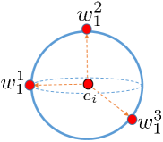
where $\gamma_{u}^{v}$ denotes the geodesic from $u$ to $v$. On such setting, we perform Eq. (11) $m$ times and obtain an initialization set for $\hat{w}_{1}$, that is, $W=\{\hat{w}_{1}^{1},{w}_{1}^{2},...,\hat{w}_{1}^{m}\}$ with $m$ candidates, covering the original $\mathcal{B}_{i}$. See Figure 5. With this degeneration, the sequential optimization of Eq. (10) is redefined as

$$\operatorname*{arg\,max}_{\hat{w}_{1}\in W}\mathcal{L}_{\mathbb{E}_{0,d}}(\hat{w}_{1}).$$ (12)

Figure 5: Vector rotation maximization. MHEAL selects the optimal ${\hat{w}}_{1}$ by observing a set of candidate ${\hat{w}}_{1}$, $t=1,2,3,...,m$, where the vector over the geodesic $\gamma_{c_{i}}^{\hat{w}_{1}^{t}}$ holds the maximal disagreement with $\gamma_{c_{i}}^{\hat{w}_{1}^{t-1}}$.

Remark 2.

With the vector rotation maximization of Eq. (11), then $\hat{w}_{1}\in\mathcal{B}_{i}$ of Eq. (10) is updated into $\hat{w}_{1}\in W$ of Eq (11). In this way, the calculation complexity of Eq. (10) degenerates into $\mathcal{O}(\frac{m^{2}N^{2}}{k^{4}})$, that is, Eq (12) results in a much lower calculation complexity after restricting $\hat{w}_{1}\in W$.

5.2 Algorithm

We present MHEAL algorithm to learn representative data, which characterizes decision boundaries in a balanced manner over each pre-estiamted hyperspherical cluster.

The detailed steps of the MHEAL algorithm are as follows. Step 3 optimizes a set of spherical clusters adopting hyperspeherical clustering w.r.t. Eq. (9), where we randomly initialize $c_{1},c_{2},c_{3},...,c_{k}$ from $\mathcal{X}$. For each hypersphere $\mathcal{B}_{i}$, Step 5 calculates the optimal initialization on $\hat{w}_{1}^{*}$ following Eq. (12), where the initialization set $W$ is obtained from Eq. (11); Steps 6 to 8 select $\tau$ data to match $\mathcal{B}_{i}$. Step 9 merges $\tau$ representative data from $\mathcal{B}_{i}$ into the representation set $\mathcal{S}$, for any $i\leq k$. In this way, the final outputs on $\mathcal{S}$ (i.e., $\mathcal{S}^{*}$) has $\tau k$ representative data, which approximately represent the $k$ spherical clusters.

1 Input: Data set $\mathcal{X}$, number of clusters $k$, number of representative data $\tau k$.

2 Initialize: Randomly initialize $c_{1},c_{2},c_{3},...,c_{k}$ from $\mathcal{X}$, and then set $\mathcal{S},\mathcal{S}^{*}=\emptyset$.

3 Solve $\operatorname*{arg\,min}_{c_{k}}\sum_{x_{i}}\Big{(}1-{\rm cos}(c_{k},x_{i})\Big{)}$.

4

5for $i=1,2,3,...,k$ do

6       $\hat{w}_{1}^{*}=\operatorname*{arg\,max}_{\hat{w}_{1}\in W}\mathcal{L}_{\mathbb{E}_{0,d}}(\hat{w}_{1})$ and $\mathcal{S}=\hat{w}_{1}^{*}$.

7       for $t=2,3,...,\tau$ do

8             $x_{t}^{*}=\operatorname*{arg\,max}_{x_{j}\in\mathcal{B}_{i}}\min_{w_{i}\in\mathcal{S}}\|w_{i}-x_{j}\|,$ $\mathcal{S}=\mathcal{S}\cup x_{t-1}^{*}$.

9       end for

10      

11      $\mathcal{S}^{*}=\mathcal{S}^{*}\cup\mathcal{S}$.

12 end for

Output: Representative set $\mathcal{S}^{*}$.

Algorithm 2 Minimizing Hyperspherical Energy-based Active Learning (MHEAL)

6 Improving Generalization for MHEAL

Section 6.1 presents the generalization analysis of MHEAL on error and label complexity bounds. Section 6.2 then presents the empirical study to explain the theoretical results.

6.1 Error and Label Complexity Bounds

MHEAL adopts a version space view that yields a clustering manner to extract representative data. This reduces the typical label complexity bound of VSAL into a set of local polynomial label complexities [54] over clusters. Here, we follow the IWAL [29] scenario to present the convergence analysis of MHEAL on the generalization error and label complexity bounds.

IWAL scenario. Given a finite hypothesis class $\mathcal{H}$, IWAL tries to update the current hypothesis $h_{t}\in\mathcal{H}$ at $t$-time into the optimal hypothesis $h^{*}\in\mathcal{H}$. Let IWAL perform $T$ rounds of querying from $\mathcal{X}$, assume that $\ell(\cdot,\cdot)$ denotes the loss of mapping $\mathcal{X}$ into $\mathcal{Y}$ with multi-class setting, we define the total loss of the $T$ rounds of querying as $R(h_{T})=\sum_{i=1}^{T}\frac{Q_{t}}{p_{i}}\ell(h(x_{t}),y_{t})$, where $y_{t}$ denotes the label of $x_{t}$, $Q_{t}$ satisfies the Bernoulli distribution of $Q_{t}\in\{0,1\}$, and $\frac{1}{p_{i}}$ denotes the weight of sampling $x_{t}$. The sampling process adopts an error disagreement to control the hypothesis updates:

$$\theta_{\rm IWAL}=\mathbb{E}_{x_{t}\in\mathcal{X}}\mathop{{\rm sup}}\limits_{h\in B(h^{*},r)}\left\{\frac{\ell(h(x_{t}),\mathcal{Y})-\ell(h^{*}(x_{t}),\mathcal{Y})}{r}\right\},$$ (13)

where $B(h^{*},r)$ denotes the ball with a center $h^{*}$ and radius $r$. In hypothesis class, $\ell(h(x_{t}),\mathcal{Y})-\ell(h^{*}(x_{t}),\mathcal{Y})$ denotes the maximal hypothesis disagreement over the loss $\ell$. On this setting, $\theta_{\rm IWAL}$ denotes the minimal step on the significant update of hypothesis. Once the hypothesis update w.r.t. error after adding $x_{t}$ is larger than $\theta_{\rm IWAL}$, IWAL solicits $x_{t}$ as a significant update. Otherwise, $x_{t}$ will not be an ideal update.

MHEAL scenario. Given the input dataset $\mathcal{X}$ with $n$ samples, it is divided into $k$ clusters: $\{\mathcal{B}_{1},\mathcal{B}_{2},...,\mathcal{B}_{k}\}$, where $\mathcal{B}_{i}$ has $N_{i}$ samples. MHEAL performs IWAL for any $\mathcal{B}_{i}$. Specifically, MHEAL uses a new error disagreement $\theta_{\rm MHEAL}$ to control the hypothesis updates:

$$\theta_{\rm MHEAL}=\mathbb{E}_{x_{t}\in\mathcal{B}_{i}}\mathop{{\rm sup}}\limits_{h\in B(h^{*},r)}\left\{\frac{\ell(h(x_{t}),\mathcal{Y})-\ell(h^{*}(x_{t}),\mathcal{Y})}{r}\right\}.$$ (14)

Theorem 1.

Given $T$ rounds of querying by employing IWAL, let $\mathcal{Q}$ be the number of ground-truth queries, i.e., label complexity. If MHEAL performs IWAL for any $\mathcal{B}_{i}$, each cluster will have $\tau=T/k$ rounds of querying. Then, with a probability at least $1-\delta$, for all $\delta>0$, for any $T>0$, the error disagreement of $R(h_{\tau})$ and $R(h^{*})$ of MHEAL is bounded by $k$ times of polynomial label complexities over each cluster

$$\begin{split}&R(h_{\tau})-R(h^{*})\\ &\leq k\times\max_{\mathcal{H}_{i},i=1,...,k}\Bigg{\{}\frac{2}{\tau}\Bigg{[}\sqrt{\sum_{t=1}^{\tau}p_{t}}+6\sqrt{{\rm log}\Big{[}\frac{2(3+\tau)\tau^{2}}{\delta}\Big{]}}\Bigg{]}\\ &\times\sqrt{{\rm log}\Big{[}\frac{16\tau^{2}|\mathcal{H}_{i}|^{2}{\rm log}\tau}{\delta}\Big{]}}\Bigg{\}}.\end{split}$$

Then, with a probability at least $1-2\delta$, for all $\delta>0$, the label complexity of MHEAL can be bounded by

$$\begin{split}&\mathcal{Q}\leq 8k\times\max_{\mathcal{H}_{i},i=1,...,k}K_{\ell}\Bigg{\{}\Big{[}\sum_{j=1}^{N_{i}}\theta_{\rm MHEAL}R_{j}^{*}\tau p_{j}\Big{]}\\ &\ \ +\sum_{j=1}^{N_{i}}O\Bigg{(}\sqrt{R_{j}^{*}\tau p_{j}{\rm log}\Big{[}\frac{\tau|\mathcal{H}_{i}|N_{i}}{\delta}\Big{]}}\Bigg{)}\!+\!O\Bigg{(}N_{i}{\rm log}^{3}\Big{(}\frac{\tau|\mathcal{H}_{i}|N_{i}}{\delta}\Big{)}\Bigg{)}\Bigg{\}}\end{split}$$

where $K_{f}$ is the slope asymmetry over the limited loss $\ell$ on $\mathcal{B}_{i}$, i.e. $\ell_{\mathcal{B}_{i}}$, $K_{f}=\mathop{{\rm sup}}\limits_{x_{t}^{\prime},x_{t}\in\mathcal{B}_{i}}\left|\frac{{\rm max}\ \ell_{\mathcal{B}_{i}}(h(x_{t}),\mathcal{Y})-\ell_{\mathcal{B}_{i}}(h(x_{t}^{\prime}),\mathcal{Y})}{{\rm min}\ \ell_{\mathcal{B}_{i}}(h(x_{t}),\mathcal{Y})-\ell_{\mathcal{B}_{i}}(h(x_{t}^{\prime}),\mathcal{Y})}\right|$, $R_{j}^{*}$ denotes the best-in-class risk at $j$-time querying, and $|\mathcal{H}|$ denotes the element number of $\mathcal{H}$ ($\ell_{0}$-norm).

6.2 Empirical Study

Datasets selection Following Cortes’s work in [54], we select six UCI datasets for our empirical study, including skin, shuttle, magic04, jm1, covtype, and nomao.

Hypotheses generation We take logistic loss defined by $\log(1+\exp(-yh(x)))$ as the hypothesis prototype. For $d$-dimensional data space, we randomly generate $10,000$ $d$-dimensional hyperplanes with a prototype of $\sum_{i}^{n}w_{i}x_{i}+b=0$, where any $w_{i}\in\mathcal{N}(0,1)$, $b$ also follows, and $h^{*}$ is defined as that hyperplane which generates the minimum loss. Note that $\mathcal{N}(0,1)$ denotes a standard Gaussian distribution.

Specification on $\theta_{\rm IWAL}$ and $\theta_{\rm MHEAL}$ With Theorem 1, we know the error disagreement of MHEAL is a tighter polynomial expression of IWAL. We thus need to specify $\theta_{\rm IWAL}$ and $\theta_{\rm MHEAL}$ which satisfy $\theta_{\rm MHEAL}\leq\theta_{\rm IWAL}$. Recalling Eqs. (11) and (12), we know 1) $\ell(h(x_{t}),\mathcal{Y})-\ell(h^{*}(x_{t}),\mathcal{Y})\leq 1$, and 2) $\ell(h(x_{t}),\mathcal{Y})-\ell(h^{*}(x_{t}),\mathcal{Y})$ of learning from $\mathcal{X}$ is tighter than that of learning from $\mathcal{B}_{i}$ since $\mathcal{B}_{i}\subset\mathcal{X}$. Let ${\rm Vol}(\cdot)$ denote the volume function, we know ${\rm Vol}(\mathcal{B_{i}})={\rm Vol}(\mathcal{X})$. Let $\xi^{\rm IWAL}_{t}=\ell(h(x_{t}),\mathcal{Y})-\ell(h^{*}(x_{t}),\mathcal{Y})$ and Let $\xi^{\rm MHEAL}_{t}=\ell(h(x_{t}),\mathcal{Y})-\ell(h^{*}(x_{t}),\mathcal{Y})$, we know $\xi^{\rm MHEAl}_{t}=\frac{1}{k}\xi^{\rm IWAL}_{t}$. To enlarge the disagreement of $\theta_{\rm IWAL}$ and $\theta_{\rm MHEAL}$, we force $\xi^{\rm IWAL}_{t}$ arrive at its upper bound, that is, $\xi^{\rm IWAL}_{t}=1$. Given a radius $r=0.1$, we then specify $\theta_{\rm IWAL}=10$. Given that there are three clusters in $\mathcal{X}$, i.e., $k=3$, with the condition of $\xi^{\rm MHEAL}_{t}=\frac{1}{k}\xi^{\rm IWAL}_{t}$, we then know $\xi^{\rm IWLA}_{t}=\frac{1}{3}\times 1=0.3333$. With a same setting on $r=0.1$, we then know $\theta_{\rm MHEAL}=3.333$.

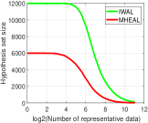
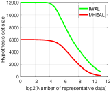
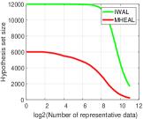
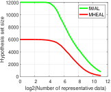
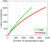
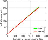
Hypothesis-pruning We start the hypothesis-pruning using $\theta_{\rm IWAL}$ and $\theta_{\rm MHEAL}$, where the pruning condition is that any hypothesis update needs to satisfy a minimal disagreement. Following [54], we invoke a feasible pruning manner to prune those $10,000$ hyperplanes, which can guarantee a near-optimal convergence. The specified way is to iteratively update $\theta_{\rm IWAL}$ and $\theta_{\rm MHEAL}$ using $\sqrt{10/t}$ for IWAL and $\sqrt{3.333/t}$ for MHEAL to eliminate more loose hypotheses. The specified pruning operation is to eliminate the hyperplane which holds a logistic loss looser than $\sqrt{10/t}$ for IWAL or $\sqrt{3.333/t}$ for MHEAL will be eliminated. Figure 6 presents the comparison of MHEAL and IWAL on their hypothesis-pruning speeds. The results show that MHEAL can prune the hypothesis class faster than typical IWAL.

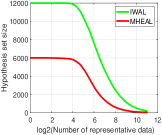
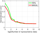
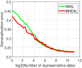
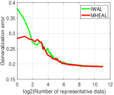
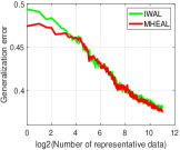
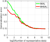
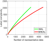
Generalization on error Error disagreement of MHEAL is a tighter polynomial expression of IWAL, which prunes the hypothesis faster. We thus study its hypothesis-pruning speed, that is, whether MHEAL can eliminate more insignificant hypotheses using a given coefficient. We thus follow the specification on $\theta_{\rm IWAL}$ and $\theta_{\rm MHEAL}$, and present the generalization error of pruning those $10,000$ hypotheses into their optimal hypothesis. The error curves are presented in Figure 7. The results show that MHEAL can obtain a tighter error than IWAL.

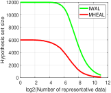
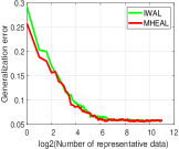
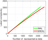
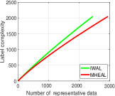
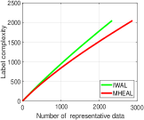
Generalization on label complexity Label complexity bound of MHEAL is also a tighter polynomial expression of IWAL. We thus try to observe their label costs of converging into a desired hypothesis. Figure 8 presents the label complexities of IWAL and MHEAL. The results show that MHEAL can spend fewer labels to converge than IWAL.

In conclusion, MHEAL employs a tighter error disagreement coefficient than IWAL to pure the hypothesis class, but results in a faster pruning speed. The generalization results on error and label complexity then show tighter bounds than that of IWAL, which verifies our theoretical results in Theorem 1.

(a) skin

(b) shuttle

(c) magic04

(d) jm1

(e) covtype

(f) nomao

Figure 6: Hypothesis-pruning speeds of IWAL and MHEAL. The results show that MHEAL can prune the hypothesis class faster than typical IWAL.

(a) skin

(b) shuttle

(c) magic04

(d) jm1

(e) covtype

(f) nomao

Figure 7: Generalization errors of IWAL and MHEAL. The results show that MHEAL can obtain a tighter error than IWAL.

(a) skin

(b) shuttle

(c) magic04

(d) jm1

(e) covtype

(f) nomao

Figure 8: Label complexities of IWAL and MHEAL. The results show that MHEAL can spend fewer labels to converge than IWAL.

7 Experiments

According to the statement of Section 5.1, MHEAL algorithm adopts hyperspherical clustering to learn the representative data in each pre-estimated cluster. The experiments discuss the following five questions.

• Why SphericalKmeans clustering is applied? How about other spherical clustering approaches, e.g. K-means and Gaussian mixture model (GMM)?

• Why do we follow $\ell_{0}$ expression of MHE? How about $\ell_{1}$ and $\ell_{2}$ expressions of MHE?

• Why decision boundaries can characterize better representative data? What is the difference of sampling in out-version-space and in-version-space?

• Can MHEAL derive more expressive representative data than the state-of-the-art deep AL baselines?

• Can MHEAL keep solid performance against special data-efficient learning settings, such as repeated and noisy scenario?

7.1 Data-Efficient Spherical Clustering

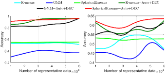
Clustering model on representative data can be transferred into large-scale learning [55]. In this section, we focus on spherical clustering on representative data, and the related baselines are K-means, GMM, and SphericalKmeans. Figure 9 presents the performance of clustering on representative data of the three baselines on MNIST and Fashion-MNIST, where the representative data are randomly sampled from the original training sets of the datasets, with a varying number from 1,000 to 6,0000. The maximum iterations of these baselines are set as 60.

To improve the non-deep clustering algorithms, we adopt the AutoEncoder and Kullback–Leibler (KL) divergence loss of deep embedding clustering (DEC) [11] to enhance their unsupervised learning results. The dimension of the input layer is 784, the encoding layers follow the (input,output) dimension settings of (784,500), (500,500), (500,2000), (2000,10), then decoding layers follow the (input,output) dimension settings of (10,2000), (2000,500), (500,500), (500,784). We also build one clustering layer, which converts the input features to label probability of clusters calculated by student’s t-distribution, measuring the similarity between embedded data and centroids.

The deep clustering results also are presented in Figure 9. It is clear that the typical clustering baselines have significant accuracy improvements by adopting AutoEncoder and DEC, where SphericalKmeans performs best most of the time whether in non-deep or deep clustering. To analyze their perturbations to the number of representative data, Table I presents the unsupervised accuracy statistics for Figure 9, where optimal accuracy denotes the best accuracy with a given number of representative data, varying from {10,000,20,000,…,60,000}, and the best ‘optimal accuracy’ and the lowest ‘standard deviation’ are marked in bold. From those metrics, we find that SphericalKmeans can achieve better clustering performance on representative data than other spherical clustering approaches, characterizing better geometric clustering features.

Figure 9: Data-efficient spherical clustering using representative data. To enhance the unsupervised learning performance of K-means, GMM, SphericalKmeans, we adopt the AutoEncoder and Kullback–Leibler (KL) divergence loss of deep embedding clustering (DEC) which performs end-to-end learning of convnets.

TABLE I: Accuracy statistics of breakpoints of the learning curves of clustering on representative data.

Algorithms	MNIST			Fashion-MNIST
	Optimal Acc	Mean Acc	Std	Optimal Acc	Mean Acc	Std
K-means	(4,0000, 0.53961)	0.5298	0.0095	(40,000, 0.55031)	0.5083	0.0372
GMM	(30000, 0.41239)	0.3695	0.0420	(50,000, 0.52611)	0.4566	0.0391
SphericalKmeans	(6,0000, 0.55188)	0.5490	0.0025	(10,000, 0.53125)	0.5262	0.0050
K-means+Auto+DEC	(60000, 0.96221)	0.9257	0.0490	(60,000, 0.62419)	0.5821	0.0309
GMM+Auto+DEC	(6,0000, 0.96256)	0.8615	0.0536	(60,000, 0.61319)	0.5743	0.0307
SphericalKmeans+Auto+DEC	(60,000, 0.96864)	0.9362	0.0172	(60,000, 0.63448)	0.6133	0.0230

7.2 Data-Efficient Distribution Matching

(a) $\ell_{\rm KL}$ on MNIST

(b) $\ell_{\rm KL}$ on F-MNIST

(c) $\ell_{\rm MMD}$ on MNIST

(d) $\ell_{\rm MMD}$ on F-MNIST

(e) ${\rm MMD}_{\mu}$ on MNIST

(f) ${\rm MMD}_{\mu}$ on F-MNIST

Figure 10: $\ell_{\rm KL}$, $\ell_{\rm MMD}$, and ${\rm MMD}_{\mu}$ loss curves of distribution matching on representative data via MHE. The curves show that distribution matching by $\ell_{0}$ MHE approximates the input distribution more tightly than $\ell_{1}$ and $\ell_{2}$ MHE. (F-MNIST denotes Fashion-MNIST )

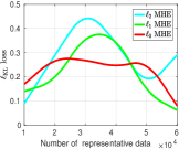
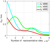
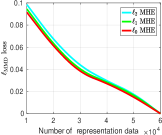
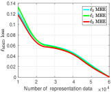
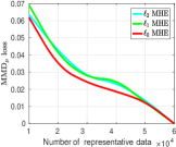
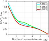
Distribution matching [56] on representative data presents expressive modeling for input features. We compare the performance disagreements of distribution matching using $\ell_{0}$, $\ell_{1}$, and $\ell_{2}$ expressions of MHE. Specifically, $\ell_{0}$ MHE minimizes $\mathbb{E}_{0,d}$ by adopting our max-min solution of Eq. (8), $\ell_{1}$ MHE minimizes $\mathbb{E}_{1,d}$ by adopting a heuristic search with a random beginning, and $\ell_{2}$ MHE minimizes $\mathbb{E}_{2,d}$ by adopting a gradient solver of Eq. (3) with a learning rate 0.001. We select KL divergence and Maximum Mean Discrepancy (MMD) [57] as the loss metrics of learning by representative data via MHE.

Given $\mathcal{X}^{\prime}$ be the representative data of $\mathcal{X}$ with a size $m$, we define $\ell_{\rm KL}:=\sum_{i}\mathcal{X}(i){\rm log}\frac{\mathcal{X}(i)}{\mathcal{X}^{\prime}(i)+\beta},$ and $\ell_{\rm MMD}:=\Big{\|}\frac{1}{n^{2}}\sum_{i,j}\|\mathcal{X}(i)-\mathcal{X}(j)\|-\frac{2}{nm}\sum_{i,j}\|\mathcal{X}(i)-\mathcal{X}^{\prime}(j)\|+\frac{1}{m^{2}}\sum_{i,j}\|\mathcal{X}^{\prime}(i)-\mathcal{X}^{\prime}(j)\|\Big{\|}_{1}^{1/2},$ where $\beta$ avoids the calculation infeasible of $\mathcal{X}^{\prime}(i)=0$, and the $\ell_{1}$ operation of $\ell_{\rm MMD}$ avoids the negative values of the $\ell_{2}$ metrics on MMD.

TABLE II: Loss statistics of the breakpoints of distribution matching on representative data via MHE.

Loss Metrics	Algorithms	MNIST			Fashion-MNIST
		Initial Loss	Mean Loss	Std	Initial Loss	Mean Loss	Std
$\ell_{\rm KL}$	$\ell_{2}$ MHE	0.1723	0.2751	0.1396	1.5013	0.4603	0.5325
	$\ell_{1}$ MHE	0.1456	0.2103	0.1331	0.5194	0.3698	0.3409
	$\ell_{0}$ MHE	0.0912	0.2183	0.0788	0.7869	0.2451	0.2788
$\ell_{\rm MMD}$	$\ell_{2}$ MHE	0.0985	0.0402	0.0354	0.1225	0.0527	0.0418
	$\ell_{1}$ MHE	0.0945	0.0338	0.0385	0.1325	0.0533	0.0455
	$\ell_{0}$ MHE	0.0915	0.0385	0.0330	0.1180	0.0494	0.0406
${\rm MMD}_{\mu}$	$\ell_{2}$ MHE	0.0634	0.0284	0.0222	0.1148	0.0410	0.0348
	$\ell_{1}$ MHE	0.0690	0.0290	0.0238	0.1039	0.0395	0.0351
	$\ell_{0}$ MHE	0.0618	0.0249	0.0212	0.1010	0.0364	0.0359

Note $\|\cdot\|_{1}$ denotes the $\ell^{1}$-norm. Since kernel MMD may result in high computational cost and has parameter perturbations, we select the unbiased $\ell_{2}$ operator to define MMD from a vector level. To approximate a nearly zero loss for $\ell_{\rm KL}$ due to its biased estimations, we set $\beta=0.552$ for MNIST and $\beta=0.352$ for Fashion-MNIST. Before estimating $\ell_{\rm KL}$ and $\ell_{\rm MMD}$, each feature of the dataset is divided by 255 which scales into [0,1]. Besides those two metrics, we also present the mean value disagreement as an overall MMD observation to verify the above two metrics: ${\rm MMD}_{\mu}=\|\mu_{\mathcal{X}}-\mu_{\mathcal{X}^{\prime}}\|$, where $\mu_{X}$ denotes the mean vector of $X$. Figures 10(a)-(d) present the loss curves of $\ell_{\rm KL}$ and $\ell_{\rm MMD}$. These curves show that distribution matching by $\ell_{0}$ MMD approximates the input distribution more tightly than $\ell_{1}$ and $\ell_{2}$ MMD.

Table 1 then presents the loss statistics of the breakpoints (e.g., {10,000, 20,000, 30,000, 40,000, 50,000, 60,000}) of Figure 10, where “Acc” denotes Accuracy and “Std” denotes Standard Deviation. The results show that $\ell_{0}$ MMD achieve lower initial and mean distribution loss than $\ell_{1}$ and $\ell_{2}$ MMD. To verify the effectiveness of $\ell_{\rm KL}$ and $\ell_{\rm MMD}$ in Figure 10, we present an overall observation by estimating ${\rm MMD}_{\mu}$ in Figures 10(e)-(f). The results keep consistent properties as with Figures 10(a)-10(d), that is, $\ell_{0}$ MHE adopting Eq. (7) usually results in lower distribution losses than its $\ell_{1}$ and $\ell_{2}$ expressions.

7.3 Data-Efficient Version Space Representation

Decision boundaries [15] are distributed in the version space over the tube manifold of hyperspherical distribution. Effective representative data are derived from decision boundaries. This section thus revels the effectiveness of MHE in characterizing the topology of decision boundaries. Following the cluster boundary detection [58] and out-of-distribution detection [59], we also use a hyper-parameterized threshold to divide one cluster into two parts: 1) in-version-space i.e. tube manifold $\mathcal{M}$, and 2) out-version-space i.e. inner regions of $B(c,R-\gamma)$. To specify $\mathcal{M}$ or $B(c,R-\gamma)$, we use hyperspherical energy as the parameterized variable.

Specification of Definition 1. Given $K$ samples around $x_{i}$, $\mathbb{E}_{0,d}(x_{i})$ denotes the hyperspherical energy of $B(c,r)$. Assume that there is a threshold $g^{\prime}$ which divides $B(c,r)$ into $\mathcal{M}$ and $B(c,R-\gamma)$: if $\mathbb{E}_{0,d}(x_{i})>g^{\prime}$, $x_{i}\in\mathcal{M}$, else $x_{i}\in B(c,R-\gamma)$. Specifically, we use PCA to project 2 dimensions of MNIST and Fashion-MNIST as its extracted features. To free $g^{\prime}$, we set $K$=5 and collect the top 30% training data with large $\mathbb{E}_{0,d}$ to specify $\mathcal{M}$.

(a) MNIST

(b) Fashion-MNIST

Figure 11: Learning disagreements of random sampling in out-of-version-space and in-version-space. The curves show that sampling representative data in in-version-space has significant superiority than that of sampling in out-of-version-space.

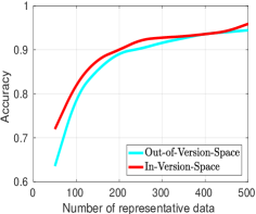
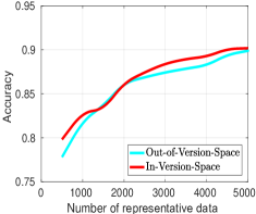
We next randomly sample representative data from $\mathcal{M}$ and $B(c,R-\gamma)$ to compare their learning disagreements. Figure 11 presents the average classification accuracy results with 10 times of random sampling, where the used prediction model is a CNN following [10]. The learning curves clearly show that sampling representative data in in-version-space has significant superiority than that of sampling in out-of-version-space. This explains our motivation of sampling representative data from in-versions-space regions, covering decision boundaries of $\gamma$-tube.

(a) Phishing

(b) Satimage

(c) Adult

(d) MNIST

Figure 12: Data-efficient learning using representative data from Phishing, Adult, Satimage, and MNIST by invoking typical active learning baselines.

TABLE III: Accuracy statistics of classification on representative data via different deep AL baselines.

Algorithms	MNIST (CNN)				CIFAR-10 (ResNet20)				CIFAR-100 (ResNet20)
	100	200	300	500	1K	2K	5K	10K	2K	5K	10K	20K
K-means [20]	0.7139	0.8752	0.9369	0.9409	0.3245	0.3889	0.5015	0.7241	0.2223	0.2631	0.3034	0.4467
K-medoids [20]	0.8465	0.9229	0.9342	0.9478	0.4794	0.5680	0.7045	0.7676	0.2625	0.3031	0.4456	0.5278
Hierarchical Tree [60]	0.8036	0.8764	0.8956	0.9123	0.5194	0.5780	0.7245	0.7636	0.2458	0.2931	0.4055	0.4674
Max Entropy [10]	0.6953	0.9056	0.9264	0.9655	0.4694	0.5480	0.6945	0.7807	0.2245	0.3031	0.4250	0.5156
Variation Ratios [10]	0.6707	0.8595	0.9226	0.9399	0.4894	0.5980	0.7418	0.7902	0.2158	0.3232	0.4301	0.5264
Core-set [61]	0.6310	0.8414	0.9035	0.9134	0.4546	0.6369	0.7403	0.7858	0.2645	0.33310	0.4654	0.5364
BALD [62]	0.7601	0.8864	0.9373	0.9636	0.5298	0.6510	0.7057	0.7764	0.2047	0.3104	0.4208	0.5298
CDAL+CoreSet [63]	0.8578	0.8972	0.9346	0.9569	0.5194	0.5780	0.6923	0.7718	0.2213	0.3031	0.4356	0.4854
CDAL+Reinforcement [63]	0.8347	0.8878	0.9232	0.9456	0.4794	0.4880	0.6202	0.7898	0.2413	0.3231	0.4351	0.4295
VAAL+VAE+Adversial [64]	0.8105	0.8502	0.9012	0.9312	0.3287	0.4021	0.6032	0.7312	0.2015	0.2878	0.3761	0.4756
MHEAL	0.8648	0.9367	0.9401	0.9785	0.5409	0.6203	0.7842	0.8146	0.3201	0.3831	0.5052	0.5505

(a) Unsupervised learning vs. MHEAL

(b) Supervised learning vs. MHEAL

(c) Deep learning vs. MHEAL

Figure 13: Data-efficient learning using representative data from MNIST. (a)Unsupervised learning vs. MHEAL. (b)Supervised learning vs. MHEAL. (c)Deep learning vs. MHEAL.

(a) Unsupervised learning vs. MHEAL

(b) Supervised learning vs. MHEAL

(c) Deep learning vs. MHEAL

Figure 14: Data-efficient learning using representative data from CIFAR10. (a)Unsupervised learning vs. MHEAL. (b)Supervised learning vs. MHEAL. (c)Deep learning vs. MHEAL.

(a) Unsupervised learning vs. MHEAL

(b) Supervised learning vs. MHEAL

(c) Deep learning vs. MHEAL

Figure 15: Data-efficient learning using representative data from CIFAR100. (a)Unsupervised learning vs. MHEAL. (b)Supervised learning vs. MHEAL. (c)Deep learning vs. MHEAL.

7.4 Data-Efficient Classification

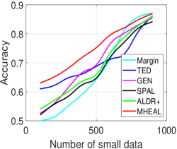
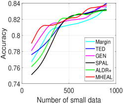
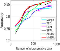
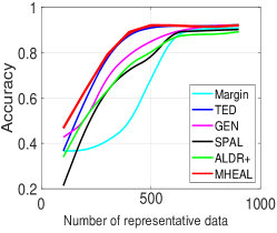
The effectiveness of learning on representative data is evaluated by active sampling from input distribution. The selected sampling baselines are Margin[65], TED [66], GEN [67], SPAL [68], ALDR+[69], and our MHEAL.

Details of the above baselines are as follows. 1) Margin selects those unlabeled data which derive the minimum margin distances. 2) Transductive experimental design (TED) selects data that represent the unlabeled data using kernel incremental tricks. 3) General AL framework (GEN) queries the samples with both representativeness and diversity. 4) Self-paced AL (SPAL) takes easiness, informativeness, and representativeness into an uniform optimization. 5) ALDR+ selects those discriminative and representative samples.

The selected experimental data are typical UCI datasets, including Phishing, Adult, Satimage, and MNIST. The used classifier tool is LIBSVM following [69]. To present fair comparison, we use SphericalK-means without AutoEncoder and DEC to perform MHEAL, and use a single query version of ALDR+. Note that Gu et al. [69] presented a bath query strategy for AL. Learning curves of these baselines with average accuracies over 100 times of running are presented in Figure 12, where the initial number of labeled data are all the class numbers of datasets. The results show that the unsupervised SphericalK-means of MHEAL has natural advantages for few labeled data. The other supervised baselines which need sufficient labels to estimate subsequent sampling, show poor performance against sufficient numbers of representative data. With the increase of the number of representative data, the performance disagreements of those baselines are reduced.

As we can observe from the above analysis, MHEAL adopts an unsupervised manner to learn on representative data, which shows expressive representation performance than those supervised methods. This helps MHEAL to actively spend tighter label complexity to converge into a desired generalization error, verifying the theoretical results of Theorem 1.

7.5 Data-Efficient Deep Classification

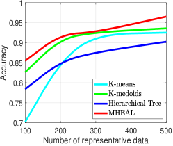
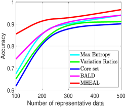
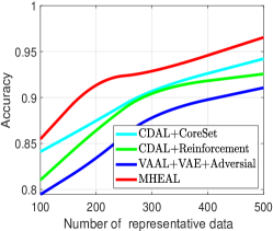
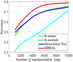
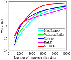
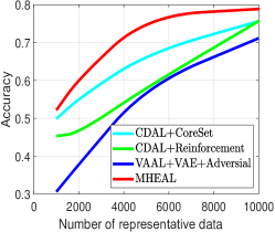
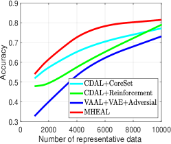
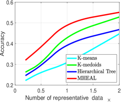
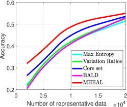
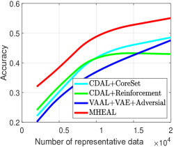
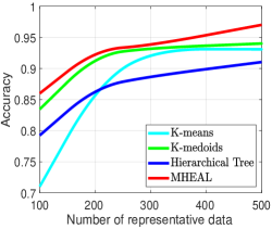
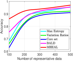
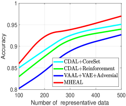
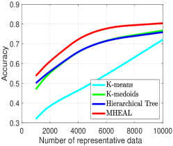
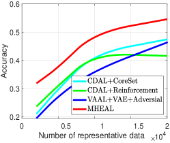
As we stated in the introduction, the typical classification learning by representative data can be implemented by AL. We thus study the classification ability with regard on representative data derived by our MHEAL and the state-of-the-art deep AL baselines. Table III presents the accuracies of classification on representative data of ten baselines on the datasets of MNIST, CIFAR-10, and CIFAR-100, respectively. For the typical AL baselines, e.g., the first seven baselines and MHEAL, training MNIST involves the Bayesian CNN of [10], and training CIFAR-10 and CIFAR-10 involve the ResNet20 of [70]. (Our experience shows that CNN has expressive modeling using few labels on MNIST.) Besides them, CDAL+CoreSet[63], CDAL+Reinforcement [63], and VAAL+VAE+Adversial [64] are set as the network architectures-based deep AL algorithms. Their details are presented as follows.

Details of network architectures-based deep AL baselines. (1) VAAL+VAE+Adversarial (VAAL: Variational adversarial active learning) [64]. It is a deep AL framework, which adopts a variational autoencoder (VAE) and an adversarial network to learn the latent space. (2) CDAL+CoreSet (CDAL: Contextual Diversity for Active Learning) [63]. This deep AL approach introduces the contextual diversity hinges to observe the probability vectors predicted by a CNN, where the vector regions of interest typically contain diverse label information. This approach cooperates with a core-set to evaluate the contextual diversity. (3) CDAL+Reinforcement (CDAL: Contextual Diversity for Active Learning) [63]. Different from CDAL+CoreSet, this deep AL approach cooperates with a reinforcement learning policy.

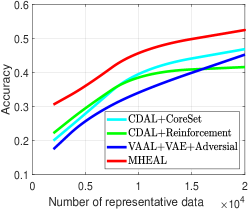
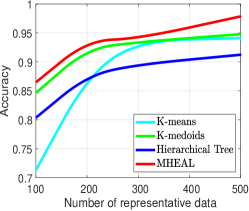
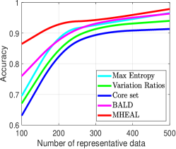
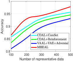
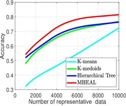
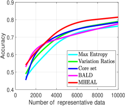
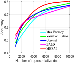
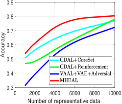
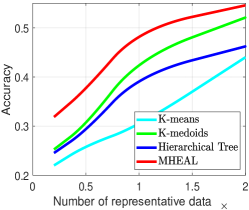
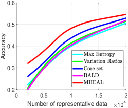
We follow [20] to select 20 random samples to initialize the hypothesis of AL. As the shown in Table III, 1) the unsupervised baselines such as K-means, K-medoids, Hierarchical Tree, and Core-set perform stably, varying the number of desired representative data, 2) the typical supervised baselines such as Max Entropy, Variation Ratios, and BALD perform not well if annotating few data; only sufficient labeled data can rapidly improve their accuracies, 3) the network architectures-based deep AL, e.g., CDAL+CoreSet and CDAL+Reinforcement, and VAAL+VAE+Adversial need large number of data and labels can show expressive modeling, while show very general accuracies among insufficient annotation budgets, 4) MHEAL employs deep clustering to extract structural clusters from the inputs, showing the state-of-the-art accuracies than other baselines on MNIST. Technically, our locally MHE optimization in each cluster yields expressive distribution matching, which derives comprehensive covering on the input features. Better accuracies then are naturally presented.

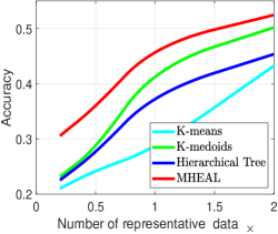
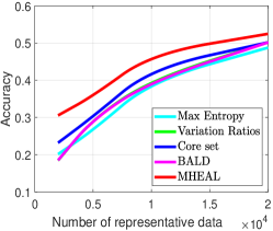
Figures 13-15 present the learning curves for Table 3. This visualizes the performance disagreement of those baselines in a different view. Compared to the experimental results of Section 7.4, those deep learning baselines need more labeled data to strength the advantages of their network configurations. However, unsupervised deep clustering does not need labels, and can obtain more useful information for subsequent MHE optimization, presenting positive guarantees.

TABLE IV: Accuracy statistics of classification on repeated representative data via different deep AL baselines.

Algorithms	MNIST (CNN)				CIFAR-10 (ResNet20)				CIFAR-100 (ResNet20)
	100	200	300	500	1K	2K	5K	10K	2K	5K	10K	20K
K-means [20]	0.7102	0.8687	0.9312	0.9309	0.3198	0.3920	0.4989	0.7210	0.2201	0.2603	0.3001	0.4401
K-medoids [20]	0.8345	0.9217	0.9330	0.9401	0.4702	0.5602	0.7102	0.7670	0.2526	0.3021	0.4405	0.5201
Hierarchical Tree [60]	0.7925	0.8698	0.8875	0.9103	0.5012	0.5623	0.7109	0.7587	0.2454	0.2901	0.4058	0.4623
Max Entropy [10]	0.6846	0.8952	0.9105	0.9567	0.4598	0.5412	0.7201	0.7712	0.2201	0.2989	0.4108	0.5058
Variation Ratios [10]	0.6608	0.8436	0.9106	0.9219	0.4802	0.5875	0.7398	0.7874	0.2048	0.3130	0.4257	0.5147
Core-set [61]	0.6293	0.8386	0.8956	0.9103	0.4501	0.6315	0.7309	0.7717	0.2587	0.3212	0.4536	0.5287
BALD [62]	0.7542	0.8798	0.9288	0.9541	0.5102	0.6426	0.6923	0.7654	0.1987	0.3026	0.4156	0.5185
CDAL+CoreSet [63]	0.8502	0.8913	0.92986	0.9510	0.5065	0.5687	0.6823	0.7689	0.2103	0.2987	0.4256	0.4745
CDAL+Reinforcement [63]	0.8298	0.8768	0.9201	0.9398	0.4687	0.4770	0.6103	0.7792	0.2365	0.3108	0.4243	0.4158
VAAL+VAE+Adversial [64]	0.8023	0.8409	0.8956	0.9269	0.3128	0.3956	0.6012	0.7226	0.1948	0.2745	0.3657	0.4635
MHEAL	0.8600	0.9302	0.9369	0.9701	0.5378	0.6156	0.7800	0.8042	0.3187	0.3745	0.4989	0.5459

7.6 Data-Efficient Deep Classification with Repeated Data

Sections 7.4 and 7.5 have presented the classification results of learning representative data by employing several state-of-the-art baselines. However, some of them depend on incremental updates of classification hypothesis, in which those updates may prefer similar or repeated samples due to the unbalanced class labels in initial data [71]. We thus consider a special scenario: data-efficient deep classification with repeated data following [71]. The goal is to test whether the baseline will be mislead by repeated data.

Following the settings of Section 7.5, we randomly select 10,000 training data and add them into the original training sets of MNIST, CIFAR10, and CIFAR100, respectively. We restart the experiments of Table 3 and report the results in Table 4. The learning curves are then represented in Figures 16 to 18 (see supplementary material). The results show that those baselines who invoke the incremental updates of hypothesis may continuously select those scarce repeated samples. However, the unsupervised baselines aim to find the representation samples, which provide fair or sufficient data for each class. It is thus that their biases are lower than those baselines using incremental updates of hypothesis.

7.7 Data-Efficient Deep Classification with Noisy Data

Learning with repeated data is inevitable. However, the tested datasets are clean data; hypothesis updates usually will be misguided by noisy labels due to their larger incremental estimations. We thus consider a more practical scenario: learning from noisy representative data. The goal is to observe the responses of those compared baselines.

Following the settings of Section 7.5, we randomly select 10,000 noisy data and add them into the original training sets of MNIST, CIFAR10, and CIFAR100, respectively. We restart the experiments of Table 3 and report the results in Table 5 (see supplementary material). The learning curves are then represented in Figures 19 to 21 (see supplementary material). The results show that those baselines who invoke the hypothesis incremental updates may be more easily misleaded by noises than clean samples. However, the unsupervised baselines use a global manner to find those representation samples, which fairly glances the samples of each class. Therefore, noisy biases of unsupervised methods are lower than supervised baselines since noises may return large perturbations to incremental updates of hypothesis.

8 Discussion

Data-efficient learning using representative data is the future trend for AI, and deep AL is one of the effective ways to implement this goal. In this work, MHE is utilized to extract representative data from the topology of decision boundaries. Deep clustering firstly provides a rough characterization for the clusters before the extraction, yielding superior performance than learning without boundary interactions.

However, such improvements depend on the clustering structures. Once the input distribution has no inherent clustering prototypes, our idea will degenerate into pure MHE optimizations in splitting regions. For real-world tasks, MHEAL will benefit the weakly-supervised [72] and semi-supervised [73] sampling issues. For noisy supervision [74], adopting our idea may reduce the wrong estimation rate on noises. Moreover, MHE optimization may bring geometric benefits for the outlier recognition and out-of-distribution detection [75]. Learning the representative data from the spherical topology, adversarial attacks [76], and malicious intrusion around the decision boundaries may be easier. Capturing the characterization of decision boundaries may fool the network filtering and mailbox defense systems.

9 Conclusion

Learning from scratch using representative data is helpful for data-efficient AI, and deep AL is one of the effective ways to implement this goal. This paper presents a novel idea of hyperspherical $\ell_{0}$ MHE from the physical geometry, to actively learn the representative data from the homeomorphic tubes of spherical manifolds. The proposed MHEAL algorithm employs deep spherical clustering, which provides a pre-estimation for the input distribution, characterizing the topology of version space. Then the max-min optimization for MHE derives effective decision boundaries to match each cluster, resulting in a lower distribution loss than $\ell_{1}$ and $\ell_{2}$ MHE. In-version-space sampling also showed more expressive modeling for classification than sampling in out-version-space, which manifests the significance of our MHEAL. Generalization error and label complexity bounds prove that MHEAL can safely converge. A series of experiment support the claimed theoretical results. In future, semi-supervised theory of MHEAL may have potential interests.

Xiaofeng Cao received his Ph.D. degree at Australian Artificial Intelligence Institute, University of Technology Sydney. He is currently an Associate Professor at the School of Artificial Intelligence, Jilin University, China and leading a Machine Perceptron Research Group with more than 15 PhD and Master students. He has published more than 10 technical papers in top tier journals and conferences, such as IEEE T-PAMI, IEEE TNNLS, IEEE T-CYB, CVPR, IJCAI, etc. In 2021, he was nominated as a rising star in “Lixin Outstanding Young Teacher Training Program of Jilin University”. In 2022, he was nominated as a candidate in “The Sixth Jilin Province Youth Science and Technology Talent Support Project”. His research interests include PAC learning theory, agnostic learning algorithm, generalization analysis, and hyperbolic geometry.

Weiyang Liu is currently conducting research at the University of Cambridge, UK and the Max Planck Institute for Intelligent Systems, Tübingen, Germany under the Cambridge-Tübingen Fellowship Program. Prior to joining this program, he has been with College of Computing, Georgia Institute of Technology, Atlanta, GA, USA. His research interests broadly lie in deep learning, representation learning, interactive machine learning and causality.

Ivor W. Tsang is Professor of Artificial Intelligence, at University of Technology Sydney. He is also the Research Director of the Australian Artificial Intelligence Institute, and an IEEE Fellow. In 2019, his paper titled “Towards ultrahigh dimensional feature selection for big data" received the International Consortium of Chinese Mathematicians Best Paper Award. In 2020, Prof Tsang was recognized as the AI 2000 AAAI/IJCAI Most Influential Scholar in Australia for his outstanding contributions to the field of Artificial Intelligence between 2009 and 2019. His works on transfer learning granted him the Best Student Paper Award at International Conference on Computer Vision and Pattern Recognition 2010 and the 2014 IEEE Transactions on Multimedia Prize Paper Award. In addition, he had received the prestigious IEEE Transactions on Neural Networks Outstanding 2004 Paper Award in 2007. Prof. Tsang serves as a Senior Area Chair for Neural Information Processing Systems and Area Chair for International Conference on Machine Learning, and the Editorial Board for Journal Machine Learning Research, Machine Learning, Journal of Artificial Intelligence Research, and IEEE Transactions on Pattern Analysis and Machine Intelligence.

Appendix

Proofs

Proof of Proposition 1.

Proof.

Given $\mathcal{L}_{\mathbb{E}_{0,d}}({\hat{w}}_{N})$ be the energy of MHE with an initial sample ${\hat{w}}_{N}$ where $\mathcal{W}=\{\hat{w}_{1},\hat{w}_{2},...,\hat{w}_{N-1}\}$, there must exist an inequality of

$$\Big{(}\prod_{N-1>i>j}\|\hat{w}_{i}-\hat{w}_{j}\|\Big{)}\times\big{(}(N-1)\min_{\hat{w}_{j}\in\mathcal{W}}\|\hat{w}_{N}-\hat{w}_{j}\|\big{)}\leq\mathcal{L}_{\mathbb{E}_{0,d}}({\hat{w}}_{N}),$$

where $\min_{\hat{w}_{j}\in\mathcal{W}}\|\hat{w}_{N}-\hat{w}_{j}\|$ denotes the minimal geodesic distance between $\hat{w}_{N}$ to the samples of $\mathcal{W}$, and $\hat{w}_{j}\in\mathcal{W}$ returns $N-1$ samples. Considering that $\min_{\hat{w}_{j}\in\mathcal{W}}\|\hat{w}_{N}-\hat{w}_{j}\|\leq\min_{\hat{w}_{i},\hat{w}_{j}\in\mathcal{W}}\|\hat{w}_{i}-\hat{w}_{j}\|$, we thus obtain an approximation of

$$\big{(}\min_{\hat{w}_{j}\in\mathcal{W}}\|\hat{w}_{N}-\hat{w}_{j}\|\big{)}^{\frac{N^{2}-3N+2}{2}}\leq\Big{(}\prod_{N-1>i>j}\|\hat{w}_{i}-\hat{w}_{j}\|\Big{)},$$

where $\prod_{N-1>i>j}$ performs $\frac{N^{2}-3N+2}{2}$ times of multiplication, there then exists

$$\big{(}\min_{\hat{w}_{j}\in\mathcal{W}}\|\hat{w}_{N}-\hat{w}_{j}\|\big{)}^{\frac{N^{2}-N}{2}}\leq\mathcal{L}_{\mathbb{E}_{0,d}}({\hat{w}}_{N}).$$

In short, given $\hat{w}_{t}$, the next observation on $\hat{w}_{t+1}$ is then specified by invoking Eq. (4). It is thus $\hat{w}_{1},\hat{w}_{2},...,\hat{w}_{N-1}$ is the optimal sequence from $\mathcal{P}$, thereby $\mathcal{L}_{\mathbb{E}_{0,d}}({\hat{w}}_{N})$ is the optimal hypersphere energy under the sequence of $\hat{w}_{1},\hat{w}_{2},...,\hat{w}_{N-1}$. On this setting, any energy under a sub-optima $\hat{w}_{N}$ is lower than $\mathcal{L}_{\mathbb{E}_{0,d}}({\hat{w}}_{N})$. Proposition 1 is then as stated. ∎

Proof of Proposition 2.

Proof.

Given $\hat{w}_{i}^{\prime},\hat{w}_{j}^{\prime}\in\mathbb{R}^{d+1}$ be the $(d+1)$-dimensional extension vector of $\hat{w}_{i},\hat{w}_{j}\in\mathbb{R}^{d}$, respectively, let $P^{\prime}$ be the $(d+1)$-dimensional extension of $P$, we know $\|\hat{w}^{\prime}_{i}-\hat{w}^{\prime}_{j}\|=\|\hat{w}_{i}-\hat{w}_{j}\|$. It is thus $\|P\hat{w}_{i}-P\hat{w}_{j}\|^{2}=\|P^{\prime}\hat{w}^{\prime}_{i}-P^{\prime}\hat{w}^{\prime}_{j}\|^{2}$ since their $(d+1)$-dimensional projections still keep zero variables. Given $d^{\prime}=d+1$, let $P^{\prime}_{id^{\prime}}$, $\hat{w}^{\prime}_{id^{\prime}}$ denote the $(d+1)$-dimension of $P^{\prime}_{i}$ and $\hat{w}_{i}^{\prime}$, respectively, there exists $P^{\prime}_{id^{\prime}}w_{id^{\prime}}=0$. With such operation, there exists $\|\hat{w}_{i}^{\prime}-\hat{w}_{j}^{\prime}\|^{2}=\|\hat{w}_{i}-\hat{w}_{j}\|^{2}$, $\|P^{\prime}\hat{w}_{i}^{\prime}-P^{\prime}\hat{w}_{j}^{\prime}\|^{2}=\|P\hat{w}_{i}-P\hat{w}_{j}\|^{2}$. Besides, $P$ and $P^{\prime}$ have a same variance. Then the inequality of Lemma 1 can be rewritten as

$$\begin{split}&{\rm Pr}\Big{\{}(1-\varepsilon)\|\hat{w}_{i}^{\prime}-\hat{w}_{j}^{\prime}\|^{2}k\sigma^{2}<\|P^{\prime}\hat{w}_{i}^{\prime}-P^{\prime}\hat{w}_{j}^{\prime}\|^{2}\\ &<(1+\varepsilon)\|\hat{w}_{i}^{\prime}-\hat{w}_{j}^{\prime}\|^{2}\kappa\sigma^{2}\Big{\}}\geq 1-2{\rm exp}\Big{(}\frac{-\kappa\varepsilon^{2}}{8}\Big{)}.\\ \end{split}$$

Because $P^{\prime}\hat{w}_{i}^{\prime}-P^{\prime}\hat{w}_{j}^{\prime}$ actually returns a $d$-dimensional vector, we thus say if $\kappa=d$, Lemma 1 then still holds. ∎

Proof of Lemma 2.

Proof.

With the same vector extension of proof of Proposition 2, for any geodesic function $d_{\mathcal{M}}\in\mathbb{R}^{d}$, it will return a zero operation on its $(d+1)-$dimensional extension. It is thus the metric of $P\hat{w}_{1},P\hat{w}_{2}$ mainly rely on their operations from 1 to $d$ dimension. Considering that $d_{\mathcal{M}}(g(w_{1}),g(w_{2})):=\nu\|w_{1}-w_{2}\|$, $d_{\mathcal{M}}(g(\hat{w}_{1}),g(\hat{w}_{2}))=\nu\Big{(}\sum_{j=1}^{N}\|\hat{w}_{1j}-\hat{w}_{2j}\|^{2}\Big{)}^{1/2}\leq\nu\Big{(}\sum_{j=1}^{N}\|\hat{w}_{2j}-\hat{w}_{3j}\|^{2}\Big{)}^{1/2}$, if $\nu=\nu^{\prime}$, there holds for $d^{\prime}_{\mathcal{M}}(g^{\prime}(w_{1}),g^{\prime}(w_{2}))=\nu^{\prime}\Big{(}\sum_{j=1}^{N}\|\hat{w}_{1j}-\hat{w}_{2j}\|^{2}\Big{)}^{1/2}\leq\nu^{\prime}\Big{(}\sum_{j=1}^{N}\|\hat{w}_{2j}-\hat{w}_{3j}\|^{2}\Big{)}$. Lemma 2 then holds. ∎

Proof of Lemma 3.

Proof.

Following [41], given a constant $e>0$, a Gaussian random projection matrix matrix $P$ leads to

$$\theta_{\mathcal{M}}(\hat{w}_{1},\hat{w}_{2})=\frac{\hat{w}_{1}^{T}\hat{w}_{2}}{\|w_{1}^{T}\|\cdot\|w_{2}^{T}\|}=\frac{1}{e}\frac{(P\hat{w}_{1})^{T}(P\hat{w}_{2})}{\|(P\hat{w}_{1})^{T}\|\cdot\|(P\hat{w}_{2})^{T}\|}.$$

Then $\theta_{\mathcal{M}}(\hat{w}_{1},\hat{w}_{2})=\frac{1}{e}\theta_{\mathcal{M}}(P\hat{w}_{1},P\hat{w}_{2})\leq\theta_{\mathcal{M}}(\hat{w}_{2},\hat{w}_{3})=\theta_{\mathcal{M}}(P\hat{w}_{2},P\hat{w}_{3}).$

With the same proof skill of Proposition 2, we extend a $d+1$ dimension vector with zero-element to $\hat{w}_{1},\hat{w}_{2},\hat{w}_{3},...,\hat{w}_{N}\in\mathbb{R}^{d+1}$ and obtain $\hat{w}_{1}^{\prime},\hat{w}_{2}^{\prime},\hat{w}_{3}^{\prime},...,\hat{w}_{N}^{\prime}\in\mathbb{R}^{d+1}$. With the Theorem 1 of [41], there exists

$$\frac{\frac{1}{e}\theta_{\mathcal{M}}(P\hat{w}_{1}^{\prime},P^{\prime}\hat{w}_{2}^{\prime})-\varepsilon}{1+\varepsilon}<\theta_{\mathcal{M}}(P^{\prime}\hat{w}_{1}^{\prime},P^{\prime}\hat{w}_{2}^{\prime})<\theta_{\mathcal{M}}(P\hat{w}_{2}^{\prime},P^{\prime}\hat{w}_{3}^{\prime})$$

With a zero operation on the $d+1$ dimension for any $\hat{w}_{i}^{\prime}$, we know $\theta_{\mathcal{M}}(P\hat{w}_{1},P\hat{w}_{2})=\theta_{\mathcal{M}}(P^{\prime}\hat{w}_{1}^{\prime},P^{\prime}\hat{w}_{2}^{\prime})$, and $\theta_{\mathcal{M}}(P^{\prime}\hat{w}_{2}^{\prime},P^{\prime}\hat{w}_{3}^{\prime})=\theta_{\mathcal{M}}(P^{\prime}\hat{w}_{2},P^{\prime}\hat{w}_{3})$, the inequality of Lemma 3 then holds.

∎

Proof of Proposition 3.

Proof.

Let $\ell_{LBM}({\hat{w}}_{N})$ denote the approximation loss of our lower bound approximation on ${\hat{w}}_{N}$. With Proposition 2, the approximation loss of Proposition 1 is given by

$$\begin{split}&\ell_{LBM}({\hat{w}}_{N})=\mathcal{L}_{\mathbb{E}_{0,d}}({\hat{w}}_{N})-\Big{(}\min_{\hat{w}_{j}\in\mathcal{W}}\|\hat{w}_{N}-\hat{w}_{j}\|\Big{)}^{\frac{N^{2}-N}{2}}\\ &\leq\Big{(}\max_{\hat{w}_{j}\in\mathcal{W}}\|\hat{w}_{N}-\hat{w}_{j}\|\Big{)}^{\frac{N^{2}-N}{2}}-\Big{(}\min_{\hat{w}_{j}\in\mathcal{W}}\|\hat{w}_{N}-\hat{w}_{j}\|\Big{)}^{\frac{N^{2}-N}{2}}.\\ \end{split}$$

We next analyze this upper bound written as $\ell^{upper}_{LBM}({\hat{w}}_{N})$. With Lemma 2.3 of [77], there exists $|x-y|^{p}\leq 2^{p-1}|x^{p}-y^{p}|,p\geq 1$. We thus control $\ell^{upper}_{LBM}({\hat{w}}_{N})$ by

$$\begin{split}&\frac{1}{\sqrt{2}^{N^{2}-N-2}}\Big{(}\max_{\hat{w}_{j}\in\mathcal{W}}\|\hat{w}_{N}-\hat{w}_{j}\|-\min_{\hat{w}_{j}\in\mathcal{W}}\|\hat{w}_{N}-\hat{w}_{j}\|\Big{)}^{\frac{N^{2}-N}{2}}\\ &\leq\ell^{upper}_{LBM}({\hat{w}}_{N})\leq\Big{(}\max_{\hat{w}_{j}\in\mathcal{W}}\|\hat{w}_{N}-\hat{w}_{j}\|\Big{)}^{\frac{N^{2}-N}{2}}.\\ \end{split}$$

Let $\ell^{upper}_{LBM}({\hat{w}}_{1:N})$ be the upper bound of the approximation loss of acquiring $N$ samples, given $\ell^{\sqrt{upper}}_{LBM}({\hat{w}}_{1:N})=\sqrt[\frac{N^{2}-N}{2}]{\ell^{upper}_{LBM}({\hat{w}}_{1:N})}$, Proposition 3 then holds. ∎

Proof of Theorem 1.

Proof.

IWAL denotes a set of observations for its weighted sampling: $\mathcal{F}_{t}=\{(x_{1},y_{1},Q_{1}),(x_{2},y_{2},Q_{2}),...,(x_{t},y_{t},Q_{t})\}$. The key step to prove Theorem 1 is to observe the martingale difference sequence for any pair $f$ and $g$ in the t-time hypothesis class $\mathcal{H}_{t}$, that is, $\xi_{t}=\frac{Q_{t}}{p_{t}}\Big{(}\ell(f(x_{t}),y_{t})-\ell(g(x_{t}),y_{t})\Big{)}-\Big{(}R(h)-R(g)\Big{)}$, where $f,g\in\mathcal{H}_{t}$. By adopting Lemma 3 of [78], with $\tau>3$ and $\delta>0$, we firstly know

$$\begin{split}&{\rm var}[\xi_{t}|\mathcal{F}_{t-1}]\\ &\leq\textbf{E}_{x_{t}}\Big{[}\frac{Q_{t}^{2}}{p_{t}^{2}}\Big{(}\ell(f(x_{t}),y_{t})\!-\!\ell(g(x_{t}),y_{t})\Big{)}\!-\!\Big{(}R(h)-R(g)\Big{)}^{2}|\mathcal{F}_{t-1}\Big{]}\\ &\leq\textbf{E}_{x_{t}}\Big{[}\frac{Q_{t}^{2}p_{t}^{2}}{p_{t}^{2}}|\mathcal{F}_{t-1}\Big{]}\\ &=\textbf{E}_{x_{t}}\Big{[}p_{t}|\mathcal{F}_{t-1}\Big{]},\\ \end{split}$$ (15)

and then there exists

$$\begin{split}&|\sum_{t=1}^{T}\xi_{t}|\\ &\leq\max_{\mathcal{H}_{i},i=1,2,...,k}\Bigg{\{}2\sqrt{\sum_{t=1}^{\tau}\textbf{E}_{x_{t}}[p_{t}|\mathcal{F}]_{t-1}},6\sqrt{{\rm log}\Big{(}\frac{8{\rm log}\tau}{\delta}\Big{)}}\Bigg{\}}\\ &\times\sqrt{{\rm log}\Big{(}\frac{8{\rm log}\tau}{\delta}\Big{)}},\\ \end{split}$$ (16)

where $\textbf{E}_{x_{t}}$ denotes the expectation over the operation on $x_{t}$. By Proposition 2 of [79], we know

$$\begin{split}&\sum_{t=1}^{\tau}\textbf{E}_{x_{t}}[p_{t}|\mathcal{F}_{t-1}]\\ &\leq\Big{(}\sum_{t=1}^{\tau}p_{t}\Big{)}+36{\rm log}\Big{(}\frac{(3+\sum_{t=1}^{\tau})\tau^{2}}{\delta}\Big{)}\\ &+2\sqrt{\Big{(}\sum_{t=1}^{\tau}p_{t}\Big{)}{\rm log}\Big{(}\frac{(3+\sum_{t=1}^{\tau})\tau^{2}}{\delta}\Big{)}}\\ &\leq\Bigg{(}\sum_{t=1}^{\tau}p_{t}+6{\rm log}\Big{(}\frac{(3+\sum_{t=1}^{\tau})\tau^{2}}{\delta}\Big{)}\Bigg{)}.\\ \end{split}$$ (17)

Introducing Eq. (17) to Eq. (16), with a probability at least $1-\delta$, we then know

$$\begin{split}&|\sum_{t=1}^{T}\xi_{t}|\\ &\leq\max_{\mathcal{H}_{i},i=1,2,...,k}\Bigg{\{}\frac{2}{\tau}\Bigg{[}\sqrt{\sum_{t=1}^{\tau}p_{t}}+6\sqrt{{\rm log}\Big{[}\frac{2(3+\tau)\tau^{2}}{\delta}\Big{]}}\Bigg{]}\\ &\times\sqrt{{\rm log}\Big{[}\frac{16\tau^{2}|\mathcal{H}_{i}|^{2}{\rm log}\tau}{\delta}\Big{]}}\Bigg{\}},\end{split}$$ (18)

For any $\mathcal{B}_{i}$, the final hypothesis converges into $h_{\tau}$, which usually holds a tighter disagreement to the optimal $h^{*}$. It is thus $R(h_{\tau})-R(h^{*})\leq|\sum_{t=1}^{\tau}\xi_{t}|$. then the error disagreement bound of Theorem 1 hold. We next prove the label complexity bound of MHEAL. Following Theorem 1, there exists

$$\begin{split}&\textbf{E}_{x_{t}}[p_{t}|\mathcal{F}_{t-1}]\\ &\leq 4\theta_{\rm IWAL}K_{\ell}\times\Bigg{(}R^{*}+\sqrt{(\frac{2}{t-1}){\rm log}(2t(t-1)|)\frac{|\mathcal{H}|^{2}}{\delta})}\Bigg{)},\\ \end{split}$$ (19)

where $R^{*}$ denotes $R(h^{*})$. Let $\sqrt{(\frac{2}{t-1}){\rm log}(2t(t-1)|)\frac{|\mathcal{H}|^{2}}{\delta})}\propto O\Big{(}{\rm log}(\frac{\tau|\mathcal{H}|}{\delta})\Big{)}$, with the proof of Lemma 4 of [54], Eq. (17) then can be approximated as

$$\begin{split}&\textbf{E}_{x_{t}}[p_{t}|\mathcal{F}_{t-1}]\\ &\leq 4\theta_{\rm IWAL}K_{\ell}\Bigg{(}\tau R^{*}+O\Big{(}R(h^{*})\tau{\rm log}(\frac{t|\mathcal{H}|}{\delta})\Big{)}+O\Big{(}{\rm log}^{3}(\frac{t|\mathcal{H}|}{\delta})\Big{)}\Bigg{)},\\ \end{split}$$ (20)

for any cluster $\mathcal{B}_{i}$, by adopting the proof of Theorem 2 of [54], we know

$$\begin{split}&\textbf{E}_{x_{t}}[p_{t}|\mathcal{F}_{t-1}]\\ &\leq 8K_{\ell}\Bigg{\{}\Big{[}\sum_{j=1}^{N_{i}}\theta_{\rm MHEAL}R_{j}^{*}\tau p_{j}\Big{]}+\sum_{j=1}^{N_{i}}O\Bigg{(}\sqrt{R_{j}^{*}\tau p_{j}{\rm log}\Big{[}\frac{\tau|\mathcal{H}_{i}|N_{i}}{\delta}\Big{]}}\Bigg{)}\!\\ &+\!O\Bigg{(}N_{i}{\rm log}^{3}\Big{(}\frac{\tau|\mathcal{H}_{i}|N_{i}}{\delta}\Big{)}\Bigg{)}\Bigg{\}}.\\ \end{split}$$ (21)

Since $\mathcal{Q}=k\times\max_{\mathcal{H}_{i}}\textbf{E}_{x_{t}}[p_{t}|\mathcal{F}_{t-1}],{\rm s.t.},i=1,2,...,k$, our analysis of Theorem 1 on $\mathcal{Q}$ holds. ∎

Experiments

(a) Unsupervised learning vs. MHEAL

(b) Supervised learning vs. MHEAL

(c) Deep learning vs. MHEAL

Figure 16: Data-efficient learning using representative data from repeated MNIST. (a)Unsupervised learning vs. MHEAL. (b) Supervised learning vs. MHEAL. (c)Deep learning vs. MHEAL.

(a) Unsupervised learning vs. MHEAL

(b) Supervised learning vs. MHEAL

(c) Deep learning vs. MHEAL

Figure 17: Data-efficient learning using representative data from repeated CIFAR-10. (a)Unsupervised learning vs. MHEAL. (b)Supervised learning vs. MHEAL. (c)Deep learning vs. MHEAL.

(a) Unsupervised learning vs. MHEAL

(b) Supervised learning vs. MHEAL

(c) Deep learning vs. MHEAL

Figure 18: Data-efficient learning from repeated CIFAR-100. (a) Unsupervised learning vs. MHEAL. (b) Supervised learning vs. MHEAL. (c) Deep learning vs. MHEAL.

TABLE V: Accuracy statistics of classification on noisy representative data via different deep AL baselines.

Algorithms	MNIST (CNN)				CIFAR-10 (ResNet20)				CIFAR-100 (ResNet20)
	100	200	300	500	1K	2K	5K	10K	2K	5K	10K	20K
K-means [20]	0.7021	0.8542	0.9210	0.9254	0.3102	0.3902	0.4878	0.7156	0.2102	0.2430	0.2814	0.4325
K-medoids [20]	0.8265	0.9102	0.9263	0.9361	0.4654	0.5523	0.7012	0.7562	0.2315	0.2816	0.4321	0.5019
Hierarchical Tree [60]	0.7842	0.8531	0.8763	0.9026	0.4958	0.5543	0.7012	0.7456	0.2251	0.2743	0.3852	0.4536
Max Entropy [10]	0.6745	0.8756	0.9026	0.9401	0.4412	0.5320	0.7019	0.7589	0.2015	0.2656	0.3987	0.4875
Variation Ratios [10]	0.6510	0.8302	0.9064	0.9108	0.4657	0.5658	0.7198	0.7687	0.1846	0.2965	0.4016	0.5021
Core-set [61]	0.6184	0.8256	0.8874	0.9010	0.4402	0.6218	0.7215	0.7650	0.2321	0.3025	0.4326	0.5016
BALD [62]	0.7412	0.8654	0.9152	0.9401	0.5003	0.6287	0.6781	0.7463	0.1852	0.2965	0.3978	0.5016
CDAL+CoreSet [63]	0.8410	0.8745	0.9103	0.9421	0.4985	0.5523	0.6714	0.7563	0.1998	0.2785	0.4135	0.4685
CDAL+Reinforcement [63]	0.8103	0.8654	0.9108	0.9256	0.4530	0.4612	0.5814	0.7563	0.2216	0.2965	0.4018	0.4158
VAAL+VAE+Adversial [64]	0.7945	0.8325	0.8847	0.9106	0.3062	0.3785	0.5874	0.7113	0.1746	0.2625	0.3457	0.4523
MHEAL	0.8548	0.9210	0.9263	0.9654	0.5214	0.6050	0.7712	0.7885	0.3056	0.3578	0.4716	0.5246

(a) Unsupervised learning vs. MHEAL

(b) Supervised learning vs. MHEAL

(c) Deep learning vs. MHEAL

Figure 19: Data-efficient learning using representative data from noisy MNIST. (a)Unsupervised learning vs. MHEAL. (b)Supervised learning vs. MHEAL. (c)Deep learning vs. MHEAL.

(a) Unsupervised learning vs. MHEAL

(b) Supervised learning vs. MHEAL

(c) Deep learning vs. MHEAL

Figure 20: Data-efficient learning using representative data from noisy CIFAR-10. (a)Unsupervised learning vs. MHEAL. (b)Supervised learning vs. MHEAL. (c)Deep learning vs. MHEAL.

(a) Unsupervised learning vs. MHEAL

(b) Supervised learning vs. MHEAL

(c) Deep learning vs. MHEAL

Figure 21: Data-efficient learning using representative data from noisy CIFAR-100. (a)Unsupervised learning vs. MHEAL. (b)Supervised learning vs. MHEAL. (c)Deep learning vs. MHEAL.

References

- [1] Y. LeCun, Y. Bengio, and G. Hinton, “Deep learning,” nature, vol. 521, no. 7553, pp. 436–444, 2015.
- [2] A. Krizhevsky, I. Sutskever, and G. E. Hinton, “Imagenet classification with deep convolutional neural networks,” Advances in neural information processing systems, vol. 25, 2012.
- [3] A. Vaswani, N. Shazeer, N. Parmar, J. Uszkoreit, L. Jones, A. N. Gomez, Ł. Kaiser, and I. Polosukhin, “Attention is all you need,” Advances in neural information processing systems, vol. 30, 2017.
- [4] D. Amodei, S. Ananthanarayanan, R. Anubhai, J. Bai, E. Battenberg, C. Case, J. Casper, B. Catanzaro, Q. Cheng, G. Chen et al., “Deep speech 2: End-to-end speech recognition in english and mandarin,” in International conference on machine learning. PMLR, 2016, pp. 173–182.
- [5] D. E. O’Leary, “Artificial intelligence and big data,” IEEE intelligent systems, vol. 28, no. 2, pp. 96–99, 2013.
- [6] A. Labrinidis and H. V. Jagadish, “Challenges and opportunities with big data,” Proceedings of the VLDB Endowment, vol. 5, no. 12, pp. 2032–2033, 2012.
- [7] M. Campbell, A. J. Hoane Jr, and F.-h. Hsu, “Deep blue,” Artificial intelligence, vol. 134, no. 1-2, pp. 57–83, 2002.
- [8] F.-Y. Wang, J. J. Zhang, X. Zheng, X. Wang, Y. Yuan, X. Dai, J. Zhang, and L. Yang, “Where does alphago go: From church-turing thesis to alphago thesis and beyond,” IEEE/CAA Journal of Automatica Sinica, vol. 3, no. 2, pp. 113–120, 2016.
- [9] Y. Wang, Q. Yao, J. T. Kwok, and L. M. Ni, “Generalizing from a few examples: A survey on few-shot learning,” ACM Computing Surveys (CSUR), vol. 53, no. 3, pp. 1–34, 2020.
- [10] Y. Gal, R. Islam, and Z. Ghahramani, “Deep bayesian active learning with image data,” in International Conference on Machine Learning. PMLR, 2017, pp. 1183–1192.
- [11] J. Xie, R. Girshick, and A. Farhadi, “Unsupervised deep embedding for clustering analysis,” in International conference on machine learning. PMLR, 2016, pp. 478–487.
- [12] Z. Zhong, L. Zheng, G. Kang, S. Li, and Y. Yang, “Random erasing data augmentation,” in Proceedings of the AAAI conference on artificial intelligence, vol. 34, no. 07, 2020, pp. 13 001–13 008.
- [13] L. Liu, M. Muelly, J. Deng, T. Pfister, and L.-J. Li, “Generative modeling for small-data object detection,” in Proceedings of the IEEE/CVF International Conference on Computer Vision, 2019, pp. 6073–6081.
- [14] W. Li, G. Dasarathy, K. Natesan Ramamurthy, and V. Berisha, “Finding the homology of decision boundaries with active learning,” Advances in Neural Information Processing Systems, vol. 33, 2020.
- [15] A. Beygelzimer, D. Hsu, J. Langford, and T. Zhang, “Agnostic active learning without constraints,” in Proceedings of the 23rd International Conference on Neural Information Processing Systems-Volume 1, 2010, pp. 199–207.
- [16] S. Hanneke, “A bound on the label complexity of agnostic active learning,” in Proceedings of the 24th international conference on Machine learning, 2007, pp. 353–360.
- [17] A. Beygelzimer, D. Hsu, N. Karampatziakis, J. Langford, and T. Zhang, “Efficient active learning,” in ICML 2011 Workshop on On-line Trading of Exploration and Exploitation. Citeseer, 2011.
- [18] W. Liu, R. Lin, Z. Liu, L. Liu, Z. Yu, B. Dai, and L. Song, “Learning towards minimum hyperspherical energy,” Advances in Neural Information Processing Systems, vol. 31, pp. 6222–6233, 2018.
- [19] S. Ben-David and U. Von Luxburg, “Relating clustering stability to properties of cluster boundaries,” in 21st Annual Conference on Learning Theory (COLT 2008). Omnipress, 2008, pp. 379–390.
- [20] X. Cao and I. W. Tsang, “Shattering distribution for active learning,” IEEE Transactions on Neural Networks and Learning Systems, 2020.
- [21] S. Hanneke et al., “Theory of disagreement-based active learning,” Foundations and Trends® in Machine Learning, vol. 7, no. 2-3, pp. 131–309, 2014.
- [22] C. Cortes, G. DeSalvo, C. Gentile, M. Mohri, and N. Zhang, “Adaptive region-based active learning,” in International Conference on Machine Learning. PMLR, 2020, pp. 2144–2153.
- [23] C. Cortes, G. DeSalvo, M. Mohri, N. Zhang, and C. Gentile, “Active learning with disagreement graphs,” in International Conference on Machine Learning. PMLR, 2019, pp. 1379–1387.
- [24] N. Roy and A. McCallum, “Toward optimal active learning through monte carlo estimation of error reduction,” ICML, Williamstown, pp. 441–448, 2001.
- [25] M.-F. Balcan, A. Beygelzimer, and J. Langford, “Agnostic active learning,” Journal of Computer and System Sciences, vol. 75, no. 1, pp. 78–89, 2009.
- [26] C. Zhang and K. Chaudhuri, “Beyond disagreement-based agnostic active learning,” in NIPS, 2014.
- [27] T. K. Huang, A. Agarwal, D. Hsu, J. Langford, and R. E. Schapire, “Efficient and parsimonious agnostic active learning,” Advances in Neural Information Processing Systems, vol. 2015, pp. 2755–2763, 2015.
- [28] L. Wang, “Sufficient conditions for agnostic active learnable.” in NIPS, vol. 22. Citeseer, 2009, pp. 1999–2007.
- [29] A. Beygelzimer, S. Dasgupta, and J. Langford, “Importance weighted active learning,” in Proceedings of the 26th annual international conference on machine learning, 2009, pp. 49–56.
- [30] P. Awasthi, M. F. Balcan, and P. M. Long, “The power of localization for efficiently learning linear separators with noise,” in Proceedings of the forty-sixth annual ACM symposium on Theory of computing, 2014, pp. 449–458.
- [31] M. Kearns and M. Li, “Learning in the presence of malicious errors,” SIAM Journal on Computing, vol. 22, no. 4, pp. 807–837, 1993.
- [32] D. Angluin and P. Laird, “Learning from noisy examples,” Machine Learning, vol. 2, no. 4, pp. 343–370, 1988.
- [33] P. Massart, É. Nédélec et al., “Risk bounds for statistical learning,” The Annals of Statistics, vol. 34, no. 5, pp. 2326–2366, 2006.
- [34] M. Bowick, A. Cacciuto, D. R. Nelson, and A. Travesset, “Crystalline order on a sphere and the generalized thomson problem,” Physical Review Letters, vol. 89, no. 18, p. 185502, 2002.
- [35] W. Liu, R. Lin, Z. Liu, L. Xiong, B. Schölkopf, and A. Weller, “Learning with hyperspherical uniformity,” in International Conference On Artificial Intelligence and Statistics. PMLR, 2021, pp. 1180–1188.
- [36] W. Liu, Y. Wen, Z. Yu, M. Li, B. Raj, and L. Song, “Sphereface: Deep hypersphere embedding for face recognition,” in Proceedings of the IEEE conference on computer vision and pattern recognition, 2017, pp. 212–220.
- [37] W. Liu, Y.-M. Zhang, X. Li, Z. Yu, B. Dai, T. Zhao, and L. Song, “Deep hyperspherical learning,” Advances in neural information processing systems, vol. 30, 2017.
- [38] W. Liu, Z. Liu, Z. Yu, B. Dai, R. Lin, Y. Wang, J. M. Rehg, and L. Song, “Decoupled networks,” in Proceedings of the IEEE Conference on Computer Vision and Pattern Recognition, 2018, pp. 2771–2779.
- [39] B. Chen, W. Liu, Z. Yu, J. Kautz, A. Shrivastava, A. Garg, and A. Anandkumar, “Angular visual hardness,” in International Conference on Machine Learning. PMLR, 2020, pp. 1637–1648.
- [40] A. Lou, I. Katsman, Q. Jiang, S. Belongie, S.-N. Lim, and C. De Sa, “Differentiating through the fréchet mean,” in International Conference on Machine Learning. PMLR, 2020, pp. 6393–6403.
- [41] R. Lin, W. Liu, Z. Liu, C. Feng, Z. Yu, J. M. Rehg, L. Xiong, and L. Song, “Regularizing neural networks via minimizing hyperspherical energy,” in Proceedings of the IEEE/CVF Conference on Computer Vision and Pattern Recognition, 2020, pp. 6917–6927.
- [42] J. Perez-Lapillo, O. Galkin, and T. Weyde, “Improving singing voice separation with the wave-u-net using minimum hyperspherical energy,” in ICASSP 2020-2020 IEEE International Conference on Acoustics, Speech and Signal Processing (ICASSP). IEEE, 2020, pp. 3272–3276.
- [43] N. Shah and D. M. Agrawal, “Impact of minimum hyperspherical energy regularization on time-frequency domain networks for singing voice separation,” in 2020 Asia-Pacific Signal and Information Processing Association Annual Summit and Conference (APSIPA ASC). IEEE, 2020, pp. 727–733.
- [44] X. Li, D. Chang, Z. Ma, Z.-H. Tan, J.-H. Xue, J. Cao, J. Yu, and J. Guo, “Oslnet: Deep small-sample classification with an orthogonal softmax layer,” IEEE Transactions on Image Processing, vol. 29, pp. 6482–6495, 2020.
- [45] W. Liu, R. Lin, Z. Liu, J. M. Rehg, L. Paull, L. Xiong, L. Song, and A. Weller, “Orthogonal over-parameterized training,” in Proceedings of the IEEE/CVF Conference on Computer Vision and Pattern Recognition, 2021, pp. 7251–7260.
- [46] J. Deng, J. Guo, N. Xue, and S. Zafeiriou, “Arcface: Additive angular margin loss for deep face recognition,” in Proceedings of the IEEE/CVF Conference on Computer Vision and Pattern Recognition, 2019, pp. 4690–4699.
- [47] Y. Liu, L. He, and J. Liu, “Large margin softmax loss for speaker verification,” Proc. Interspeech 2019, pp. 2873–2877, 2019.
- [48] T. Pang, K. Xu, Y. Dong, C. Du, N. Chen, and J. Zhu, “Rethinking softmax cross-entropy loss for adversarial robustness,” in International Conference on Learning Representations, 2019.
- [49] P. Mettes, E. van der Pol, and C. G. Snoek, “Hyperspherical prototype networks,” arXiv preprint arXiv:1901.10514, 2019.
- [50] W. Liu, Z. Liu, J. M. Rehg, and L. Song, “Neural similarity learning,” Advances in Neural Information Processing Systems, vol. 32, 2019.
- [51] A. Kaban, “Improved bounds on the dot product under random projection and random sign projection,” in Proceedings of the 21th ACM SIGKDD International Conference on Knowledge Discovery and Data Mining, 2015, pp. 487–496.
- [52] X. Cao and I. Tsang, “Distribution disagreement via lorentzian focal representation,” IEEE Transactions on Pattern Analysis and Machine Intelligence, 2021.
- [53] C. Buchta, M. Kober, I. Feinerer, and K. Hornik, “Spherical k-means clustering,” Journal of statistical software, vol. 50, no. 10, pp. 1–22, 2012.
- [54] C. Cortes, G. DeSalvo, C. Gentile, M. Mohri, and N. Zhang, “Region-based active learning,” in 22nd International Conference on Artificial Intelligence and Statistics, AISTATS 2019, 2020.
- [55] W. Dai, Q. Yang, G.-R. Xue, and Y. Yu, “Self-taught clustering,” in Proceedings of the 25th international conference on Machine learning, 2008, pp. 200–207.
- [56] S. Bickel, C. Sawade, and T. Scheffer, “Transfer learning by distribution matching for targeted advertising.” in NIPS, vol. 8. Citeseer, 2008, pp. 105–112.
- [57] A. Gretton, K. M. Borgwardt, M. J. Rasch, B. Schölkopf, and A. Smola, “A kernel two-sample test,” The Journal of Machine Learning Research, vol. 13, no. 1, pp. 723–773, 2012.
- [58] X. Cao, B. Qiu, X. Li, Z. Shi, G. Xu, and J. Xu, “Multidimensional balance-based cluster boundary detection for high-dimensional data,” IEEE transactions on neural networks and learning systems, vol. 30, no. 6, pp. 1867–1880, 2018.
- [59] S. Liang, Y. Li, and R. Srikant, “Enhancing the reliability of out-of-distribution image detection in neural networks,” in International Conference on Learning Representations, 2018.
- [60] S. Dasgupta and D. Hsu, “Hierarchical sampling for active learning,” in Proceedings of the 25th international conference on Machine learning, 2008, pp. 208–215.
- [61] O. Sener and S. Savarese, “Active learning for convolutional neural networks: A core-set approach,” in International Conference on Learning Representations, 2018.
- [62] N. Houlsby, F. Huszár, Z. Ghahramani, and M. Lengyel, “Bayesian active learning for classification and preference learning,” arXiv preprint arXiv:1112.5745, 2011.
- [63] S. Agarwal, H. Arora, S. Anand, and C. Arora, “Contextual diversity for active learning,” in European Conference on Computer Vision. Springer, 2020, pp. 137–153.
- [64] S. Sinha, S. Ebrahimi, and T. Darrell, “Variational adversarial active learning,” in Proceedings of the IEEE/CVF International Conference on Computer Vision, 2019, pp. 5972–5981.
- [65] S. Tong and D. Koller, “Support vector machine active learning with applications to text classification,” Journal of machine learning research, vol. 2, no. Nov, pp. 45–66, 2001.
- [66] K. Yu, J. Bi, and V. Tresp, “Active learning via transductive experimental design,” in Proceedings of the 23rd international conference on Machine learning, 2006, pp. 1081–1088.
- [67] B. Du, Z. Wang, L. Zhang, L. Zhang, W. Liu, J. Shen, and D. Tao, “Exploring representativeness and informativeness for active learning,” IEEE transactions on cybernetics, vol. 47, no. 1, pp. 14–26, 2015.
- [68] Y.-P. Tang and S.-J. Huang, “Self-paced active learning: Query the right thing at the right time,” in Proceedings of the AAAI conference on artificial intelligence, vol. 33, no. 01, 2019, pp. 5117–5124.
- [69] B. Gu, Z. Zhai, C. Deng, and H. Huang, “Efficient active learning by querying discriminative and representative samples and fully exploiting unlabeled data,” IEEE Transactions on Neural Networks and Learning Systems, 2020.
- [70] Keras, “https://keras.io/zh/examples/cifar10_resnet/.”
- [71] A. Kirsch, J. Van Amersfoort, and Y. Gal, “Batchbald: Efficient and diverse batch acquisition for deep bayesian active learning,” Advances in neural information processing systems, vol. 32, pp. 7026–7037, 2019.
- [72] Y.-F. Li, L.-Z. Guo, and Z.-H. Zhou, “Towards safe weakly supervised learning,” IEEE transactions on pattern analysis and machine intelligence, vol. 43, no. 1, pp. 334–346, 2019.
- [73] A. Gadde, A. Anis, and A. Ortega, “Active semi-supervised learning using sampling theory for graph signals,” in Proceedings of the 20th ACM SIGKDD international conference on Knowledge discovery and data mining, 2014, pp. 492–501.
- [74] A. Veit, N. Alldrin, G. Chechik, I. Krasin, A. Gupta, and S. Belongie, “Learning from noisy large-scale datasets with minimal supervision,” in Proceedings of the IEEE conference on computer vision and pattern recognition, 2017, pp. 839–847.
- [75] Y.-C. Hsu, Y. Shen, H. Jin, and Z. Kira, “Generalized odin: Detecting out-of-distribution image without learning from out-of-distribution data,” in Proceedings of the IEEE/CVF Conference on Computer Vision and Pattern Recognition, 2020, pp. 10 951–10 960.
- [76] Y. Dong, F. Liao, T. Pang, H. Su, J. Zhu, X. Hu, and J. Li, “Boosting adversarial attacks with momentum,” in Proceedings of the IEEE conference on computer vision and pattern recognition, 2018, pp. 9185–9193.
- [77] C. Qian and W. Lin, “Non-lipschitz continuous stabilizers for nonlinear systems with uncontrollable unstable linearization,” Systems & Control Letters, vol. 42, no. 3, pp. 185–200, 2001.
- [78] S. M. Kakade and A. Tewari, “On the generalization ability of online strongly convex programming algorithms.” in NIPS, 2008, pp. 801–808.
- [79] N. Cesa-Bianchi and C. Gentile, “Improved risk tail bounds for on-line algorithms,” IEEE Transactions on Information Theory, vol. 54, no. 1, pp. 386–390, 2008.
![[Uncaptioned image]](/html/2206.15204/assets/x46.png) |