A polyhedral approximation algorithm for recession cones of spectrahedral shadows

Abstract

The intersection of an affine subspace with the cone of positive semidefinite matrices is called a spectrahedron. An orthogonal projection thereof is called a spectrahedral shadow or projected spectrahedron. Spectrahedra and their projections can be seen as a generalization of polyhedra. This article is concerned with the problem of approximating the recession cones of spectrahedra and spectrahedral shadows via polyhedral cones. We present two iterative algorithms to compute outer and inner approximations to within an arbitrary prescribed accuracy. The first algorithm is tailored to spectrahedra and is derived from polyhedral approximation algorithms for compact convex sets and relies on the fact, that an algebraic description of the recession cone is available. The second algorithm is designed for projected spectrahedra and does not require an algebraic description of the recession cone, which is in general more difficult to obtain. We prove correctness and finiteness of both algorithms and provide numerical examples.

1 Introduction

Polyhedral approximation is a common technique used in mathematical programming. It is, e.g., used in algorithms that approximate the feasible region of a convex optimization problem by a sequence of polyhedra in order to obtain an approximate solution. Early publications of these algorithms include, amongs others, Cheney’s and Goldstein’s Newton method for convex programming [8], Kelley’s cutting-plane method [29], and Veinott’s supporting hyperplane method [53]. These algorithms have since been improved and extended in various directions and different fields, such as global optimization [51, 52], geometry [33], solution concepts for multiple objective optimization problems [49, 24, 14, 36], and algorithms for mixed-integer convex optimization problems [12, 54, 32]. Kamenev unites the approximation ideas in the above mentioned works into a family of iterative algorithms called augmenting and cutting schemes [26] and analyzes their efficiency and convergence properties in [27, 28].

Interest in polyhedral approximations arise from the fact that, while polyhedra do not have to be finite sets, they can be represented in a finite manner and many set calculus operations can be performed with them straightforwardly, see [10]. This makes them particularly suitable for computer-aided treatment and easier to work with than with more general convex sets.

The algorithms mentioned so far are tailored to compact sets, because unbounded sets can only be approximated by polyhedra in the Hausdorff distance if they satisfy restrictive properties as investigated in [41]. However, unbounded sets arise naturally in applications. In the theory of convex vector optimization, for example, there exists a solution concept, that is based on finding a polyhedral approximation of the so-called extended feasible image of the problem. This set is unbounded by its construction, but it is advantageous to work with it rather than with the possibly bounded feasible image, because its boundary satisfies certain minimality properties, see [34, 14]. The recession cone of a set describes its asymptotic behaviour and is therefore a crucial characteristic in the study of unbounded sets. In order to properly deal with unboundedness in the framework of polyhedral approximation, the recession cone of the given set should be approximated in some sense. There are several ways to define metrics on the space of closed and convex cones, which are summarized in the survey article [25].

Spectrahedra are intersections of affine subspaces with the cone of positive semidefinite matrices and can be defined by affine matrix inequalities. Projections of spectrahedra are called projected spectrahedra, spectrahedral shadows or semidefinitely-representable sets and arise as the feasible regions of semidefinite programs. Hence, they are ubiquitous in modern optimization. They can be viewed as a generalization of polyhedra, as they contain the class of polyhedral sets as a proper subclass and as they are closed under many operations under which polyhedra are also closed, see e.g. [40]. One aspect in which spectrahedra and their projections differ from each other is the difficulty in expressing their recession cones. While the recession cone of a spectrahedron can be described by the linear part of the defining matrix inequality, there is no straightforward way to describe the recession cone of a projected spectrahedron from its data.

This manuscript is concerned with the task of computing polyhedral approximations of the recession cones of specrahedra and spectrahedral shadows. To the best of the authors knowledge, there do not exist any algorithms in the literature tailored to this problem. We present two iterative approximations algorithms for recession cones. The first one is designed for spectrahedra and is derived from augmenting and cutting schemes. A key requirement for this algorithm is that an algebraic description of the recession cone is known. The second algorithm does not require prior knowledge about the whole recession cone, but only a single element must be known. It is suitable for the approximation of the recession cone of a spectrahedral shadow. Both algorithms compute polyhedral inner and outer approximations to within a prescribed accuracy. We show that the algorithms are correct and finite, given that the input set contains no lines and has a solid recession cone. The algorithms are tested and compared on three examples.

The article is structured as follows. In Section 2 we introduce the necessary notation and definitions. Section 3 is devoted to the polyhedral approximation of recession cones of spectrahedra. After reciting some results about convex cones and presenting first results about relevant semidefinite optimization problems, the first algorithm is presented. Thereafter, its correctness and finiteness is proved. The algorithm for the approximation of recession cones of spectrahedral shadows is provided in Section 4. Again, we prove correctness and finiteness. In the final section, we test both algorithm on examples.

2 Preliminaries

Given a set $C\subseteq\mathbb{R}^{n}$, we denote by $\operatorname{conv}C$, $\operatorname{cone}C$, $\operatorname{int}C$, $\operatorname{bd}C$ and $\operatorname{cl}C$ the convex hull, conical hull, interior, boundary, and closure of $C$, respectively. The Minkowski addition between two sets $C_{1}$ and $C_{2}\subseteq\mathbb{R}^{n}$ is defined as $C_{1}+C_{2}:=\left\{{c_{1}+c_{2}\mid c_{1}\in C_{1},c_{2}\in C_{2}}\right\}.$ A set $K$ is called a cone, if $x\in K$ implies $\alpha x\in K$ for every $\alpha\geq 0$. A cone $K$ is called pointed, if $K\cap(-K)=\left\{{0}\right\}$. The set

$$\left\{{d\in\mathbb{R}^{n}\mid x\in C\Rightarrow x+d\in C}\right\},$$

denoted by $\operatorname{0^{\infty}}C$, is called the recession cone of the convex set $C$. A closed convex set is called line-free, if its recession cone is pointed. The polar cone of a convex cone $K\subseteq\mathbb{R}^{n}$ is defined as $\left\{{x\in\mathbb{R}^{n}\mid y\in K\Rightarrow x^{\mathsf{T}}y\leq 0}\right\}$ and denoted by $K^{\circ}$. A polyhedron $P\subseteq\mathbb{R}^{n}$ is defined as the intersection of finitely many closed halfspaces, i.e. $P=\left\{{x\in\mathbb{R}^{n}\mid Ax\leq b}\right\}$ for some $A\in\mathbb{R}^{m\times n}$, $b\in\mathbb{R}^{m}$, and $m\in\mathbb{N}$. The tuple $(A,b)$ is called a H-representation or halfspace representation of $P$. Alternatively, $P$ can also be expressed as the Minkowski sum of the convex hull of finitely many points and the conical hull of finitely many directions, i.e. there exist $k,\ell\in\mathbb{N}$, points $v_{1},\dots,v_{k}\in\mathbb{R}^{n}$, and unit directions $d_{1},\dots,d_{\ell}\in\mathbb{R}^{n}$, such that $P=\operatorname{conv}\left\{{v_{i}\mid i=1,\dots,k}\right\}+\operatorname{cone}\left\{{d_{j}\mid j=1,\dots,\ell}\right\}$. In this connection, we use the convention $\operatorname{conv}\emptyset=\emptyset$ and $\operatorname{cone}\emptyset=\left\{{0}\right\}$. Given the matrices $V\in\mathbb{R}^{n\times k}$ and $D\in\mathbb{R}^{n\times\ell}$, where the $i$-th column of $V$ is $v_{i}$ and the $j$-th column of $D$ is $d_{j}$, we call the tuple $(V,D)$ a V-representation or vertex representation of $P$. If the sets $\left\{{v_{i}\mid i=1,\dots,k}\right\}$ and $\left\{{d_{j}\mid j=1,\dots,\ell}\right\}$ are minimal in the sense that no proper subset of any of the sets generates the same polyhedron, then we call the $v_{i}$ vertices of $P$ and the $d_{j}$ extreme directions of $P$. The well-known Minkowski-Weyl theorem states that every polyhedron admits both an H- and a V-representation. Given a hyperplane $H(w,\gamma)$ with normal vector $w$ and offset $\gamma$, i.e. $H(w,\gamma)=\left\{{x\in\mathbb{R}^{n}\mid w^{\mathsf{T}}x=\gamma}\right\}$, we denote the corresponding halfspace $\left\{{x\in\mathbb{R}^{n}\mid w^{\mathsf{T}}x\leq\gamma}\right\}$ by $H^{-}(w,\gamma)$. Moreover, we say that a hyperplane $H(w,\gamma)$ supports a set $C\subseteq\mathbb{R}^{n}$ or is a supporting hyperplane of $C$, if $C\subseteq H^{-}(w,\gamma)$ and $C\cap H(w,\gamma)\neq\emptyset$.

We write $e_{i}$ for the $i$-th standard unit vector in $\mathbb{R}^{n}$ and $e$ for the vector whose components are all equal to one. The Euclidean norm of a vector $x\in\mathbb{R}^{n}$ is written as $\left\lVert{x}\right\rVert$. The vector space of real symmetric $n\times n$ matrices is denoted by $\mathcal{S}^{n}$. The identity matrix in $\mathcal{S}^{n}$ is declared $I$. If a matrix $S\in\mathcal{S}^{n}$ is positive semidefinite, we write $S\succcurlyeq 0$, and if it is positive definite, $S\succ 0$. The usual inner product on $\mathcal{S}^{n}$ is defined by $S_{1}\cdot S_{2}=\operatorname{trace}(S_{1}S_{2})$, where $S_{1}S_{2}$ means ordinary matrix multiplication. The Hausdorff distance between two sets $C_{1},C_{2}\subseteq\mathbb{R}^{n}$, denoted by $d_{\mathsf{H}}\left({C_{1}},{C_{2}}\right)$, is defined as

$$\max\left\{{\sup_{c_{1}\in C_{1}}\inf_{c_{2}\in C_{2}}\left\lVert{c_{1}-c_{2}}\right\rVert,\sup_{c_{2}\in C_{2}}\inf_{c_{1}\in C_{1}}\left\lVert{c_{2}-c_{1}}\right\rVert}\right\}.$$

It is well known that the Hausdorff distance defines a metric on the space of compact subsets of $\mathbb{R}^{n}$. However, if one argument is unbounded, the Hausdorff distance may be infinite. In particular, if $K_{1},K_{2}$ are convex cones, their Hausdorff distance is $0$ if $\operatorname{cl}K_{1}=\operatorname{cl}K_{2}$ and $+\infty$ otherwise.

The (linear matrix) pencil $\mathcal{A}$ of size $\ell$ defined by the matrices $A_{1},\dots,A_{n}\in\mathcal{S}^{\ell}$ is the linear function

$$\mathcal{A}\colon\mathbb{R}^{n}\to\mathcal{S}^{\ell},\quad\mathcal{A}(x)=\sum_{i=1}^{n}x_{i}A_{i}.$$

A pencil $\mathcal{A}$ of size $\ell$ together with a matrix $A\in\mathcal{S}^{\ell}$ define the spectrahedron

$$\left\{{x\in\mathbb{R}^{n}\mid\mathcal{A}(x)+A\succcurlyeq 0}\right\}.$$

Given two pencils $\mathcal{A}$ and $\mathcal{B}$ of size $\ell$ defined on $\mathbb{R}^{n}$ and $\mathbb{R}^{m}$, respectively, and a matrix $A\in\mathcal{S}^{\ell}$, the set

$$S:=\left\{{x\in\mathbb{R}^{n}\mid\exists y\in\mathbb{R}^{m}\colon\mathcal{A}(x)+\mathcal{B}(y)+A\succcurlyeq 0}\right\}$$

is called a projected spectrahedron or spectrahedral shadow. The set $S$ is the projection of the spectrahedron $\left\{{(x,y)\in\mathbb{R}^{n+m}\mid(\mathcal{A}+\mathcal{B})(x,y)+A\succcurlyeq 0}\right\}$ onto the $x$-variables, hence the name.

3 An approximation algorithm for recession cones of spectrahedra

In this section we present an algorithm for the computation of a polyhedral inner and outer approximation of the recession cone of a spectrahedron. The algorithm is based on augmenting and cutting schemes introduced in [26] and [7]. Augmenting and cutting schemes are iterative algorithms for compact convex sets that successively improve the polyhedral approximations. In doing so, augmenting schemes compute inner approximations and cutting schemes compute outer approximations. Their functionality can be described as follows. Assume $C\subseteq\mathbb{R}^{n}$ is the set to be approximated and $\mathcal{O}^{k}$/$\mathcal{I}^{k}$ are the polyhedral outer and inner approximations computed after iteration $k$ by a cutting and augmenting scheme, respectively. Then a cutting scheme refines $\mathcal{O}^{k}$ by

1. Choose a direction $w$.

2. Compute a supporting hyperplane $H$ of $C$ with normal vector $w$.

3. Construct $\mathcal{O}^{k+1}=\mathcal{O}^{k}\cap H^{-}$.

In an augmenting scheme the procedure can be stated as

1. Compute a point $x\in\operatorname{bd}C$.

2. Contruct $\mathcal{I}^{k+1}=\operatorname{conv}\left(\mathcal{I}^{k}\cup\left\{{x}\right\}\right)$.

These iterative schemes are also jointly called Hausdorff schemes, because the above steps are typically iterated until the Hausdorff distance between $C$ and $\mathcal{O}^{k}$/$\mathcal{I}^{k}$ is at most a predefined margin. Various algorithms using the ideas of cutting and augmenting schemes can be found in the literature, for example to approximate compact spectrahedral shadows [9] or in the realm of vector optimization [13, 3].

As we are working with cones, the Hausdorff distance is unsuitable as a measure of similarity. Therefore, we consider the following distance measure on the space of closed convex cones.

Definition 3.1 (cf. [25]).

Let $K_{1},K_{2}\subseteq\mathbb{R}^{n}$ be closed convex cones. The truncated Hausdorff distance between $K_{1}$ and $K_{2}$, denoted $\bar{d}_{\mathsf{H}}(K_{1},K_{2})$, is defined as

$$\bar{d}_{\mathsf{H}}(K_{1},K_{2}):=d_{\mathsf{H}}\left({K_{1}\cap B},{K_{2}\cap B}\right),$$

where $B:=\left\{{x\in\mathbb{R}^{n}\mid\left\lVert{x}\right\rVert\leq 1}\right\}$.

It is known that the truncated Hausdorff distance defines a metric in the space of closed convex cones in $\mathbb{R}^{n}$, see [48, 21]. Moreover, it clearly holds, that $\bar{d}_{\mathsf{H}}(K_{1},K_{2})\leq 1$ for all closed convex cones $K_{1}$, $K_{2}$.

We use the truncated Hausdorff distance to define polyhedral approximations of cones.

Definition 3.2.

Given a closed convex cone $K\subseteq\mathbb{R}^{n}$ and $\varepsilon>0$, we call a polyhedral cone $R$ an outer (inner) $\varepsilon$-approximation of $K$, if $K\subseteq R$ ($R\subseteq K$) and $\bar{d}_{\mathsf{H}}(R,K)\leq\varepsilon$.

In order to link this idea to the Hausdorff distance and work with cones in the framework of Hausdorff schemes, we need the concept of bases.

Definition 3.3.

Let $K\subseteq\mathbb{R}^{n}$ be a convex cone. A subset $M\subseteq K$ is called a base of $K$, if for every $x\in K\setminus\left\{{0}\right\}$ there exists a unique $\lambda_{x}>0$, such that $\lambda_{x}x\in M$.

The following two results establish, that every closed pointed cone admits a compact base and that such a base can be constructed via its polar cone. Proofs of these results can be found in [2, Theorem 3.5] and [31, Theorem 3.2]. There are numerous other sources that study cones and their properties, e.g., [19, 6, 20, Chapter 2].

Proposition 3.4.

Let $K\subseteq\mathbb{R}^{n}$ be a closed pointed cone. Then $\operatorname{int}K^{\circ}\neq\emptyset$.

Proposition 3.5.

Let $K\subseteq\mathbb{R}^{n}$ be a closed pointed cone. Then

$$H(w,-\gamma)\cap K$$

is a compact base of $K$ for ever $w\in\operatorname{int}K^{\circ}$ and $\gamma>0$.

As a consequence, we are able to reduce the approximation of the recession cone with respect to the truncated Hausdorff distance to the approximation of a compact base of the cone with respect to the Hausdorff distance.

Proposition 3.6.

Let $K\subseteq\mathbb{R}^{n}$ be a closed pointed cone and $w\in\operatorname{int}K^{\circ}$. Assume $P$ is a polyhedron satisfying $d_{\mathsf{H}}\left({P},{H(w,-\gamma)\cap K}\right)\leq\varepsilon$. Then the following implications hold:

1. $H(w,-\gamma)\cap K\subseteq P$, $\gamma\geq(1+\varepsilon)\left\lVert{w}\right\rVert\Rightarrow\operatorname{cone}P$ is an outer $\varepsilon$-approximation of $K$.

2. $P\subseteq H(w,-\gamma)\cap K$, $\gamma\geq(1+\varepsilon)\left\lVert{w}\right\rVert\Rightarrow\operatorname{cone}P$ is an inner $\varepsilon$-approximation of $K$.

Proof.

We begin the proof with the first assertion. By the Cauchy-Schwarz inequality it holds $\left\lVert{x}\right\rVert\geq 1+\varepsilon$ for every $x\in H(w,-\gamma)$. Taking this into account together with $d_{\mathsf{H}}\left({P},{H(w,-\gamma)\cap K}\right)\leq\varepsilon$ yields $\left\lVert{x}\right\rVert\geq 1$ for every $x\in P$. Proposition 3.5 ensures that $H(w,-\gamma)\cap K$ is a compact set and

$$K=\operatorname{cone}\left(H(w,-\gamma)\cap K\right),$$

because $H(w,-\gamma)\cap K$ is a base of $K$. Since the Hausdorff distance between $P$ and $H(w,-\gamma)\cap K$ is bounded from above, $P$ must also be compact. This guarantees that $\operatorname{cone}P$ is a polyhedral cone.

Now, assume $\bar{d}_{\mathsf{H}}(\operatorname{cone}P,K)$ is attained as $\left\lVert{p-k}\right\rVert$ for $p\in\operatorname{cone}P$ and $k\in K$. This implies, that $\left\lVert{p}\right\rVert=1$. Let $\alpha$ be chosen, such that $\alpha k\in P$. By the above remark that $\left\lVert{x}\right\rVert\geq 1$ for every $x\in P$ this implies $\alpha\geq 1$. Now it holds,

$$\bar{d}_{\mathsf{H}}(\operatorname{cone}P,K) =\left\lVert{p-k}\right\rVert$$

$$\leq\alpha\left\lVert{p-k}\right\rVert$$

$$\leq\inf_{\bar{k}\in H(w,-\gamma)\cap K}\left\lVert{\alpha p-\bar{k}}\right\rVert$$

$$\leq d_{\mathsf{H}}\left({P},{H(w,-\gamma)\cap K}\right)$$

$$\leq\varepsilon.$$

The second inequality holds true, because $\alpha k$ is the projection of $\alpha p$ onto $K$, i.e.

$$\left\lVert{\alpha p-\alpha k}\right\rVert=\inf_{\bar{k}\in K}\left\lVert{\alpha p-\bar{k}}\right\rVert.$$

To complete the proof, note that $H(w,-\gamma)\cap K\subseteq P$ implies $K\subseteq\operatorname{cone}P$, because taking the conical hull is an inclusion preserving operation. The proof of the second assertion is analogous to the first one with the roles of $P$ and $H(w,-\gamma)\cap K$ interchanged. ∎

Now, from a polyhedral approximation $P$ of a compact base of the recession cone of a spectrahedron, we obtain an approximation of the recession cone itself by constructing $\operatorname{cone}P$. Constructing the conical hull requires no other computation than transposing and concatenating the matricial data of $P$ as is shown in [10, Propositions 8, 10].

From now on we denote by $C$ the spectrahedron $C:=\left\{{x\in\mathbb{R}^{n}\mid\mathcal{A}(x)+A\succcurlyeq 0}\right\}$ for matrices $A,A_{1},\dots,A_{n}\in\mathcal{S}^{\ell}$. We consider the following semidefinite optimization problem associated with $C$ and a nonzero direction $w\in\mathbb{R}^{n}$.

$$\max\;w^{\mathsf{T}}x\quad\text{s.t.}\quad\mathcal{A}(x)+A\succcurlyeq 0 C,w$$ (P₁())

Geometrically, solving (P₁($C,w$)) amounts to determining the maximal shifting of a hyperplane with normal direction $w$ within the spectrahedron $C$. Another optimization problem we consider reads as

$$\max\;t \mathcal{A}(x)+A \succcurlyeq 0 C,c,d$$ s.t. (P₂())

$$x =c+td,$$

for a point $c\in\mathbb{R}^{n}$ and a nonzero direction $d\in\mathbb{R}^{n}$. Geometrically, given $c\in\operatorname{int}C$, a solution to (P₂($C,c,d$)) is be determined by starting at the point $c$ and moving a positive distance in the direction $d$ until a boundary point of $C$ is reached. In general, a part of a solution to (P₂($C,c,d$)), if it exists, will be a point in $\operatorname{bd}C\cap\left\{{c+td\mid t\in\mathbb{R}}\right\}$. In the field of vector optimization, problems of type (P₂($C,c,d$)) can be derived from the Tammer-Weidner functional, see [17, 18]. They also appear in the literature under the name Pascoletti-Serafini scalarization and are related to Minkowski functionals, see [44, 15, 22]. The Lagrange dual problem of (P₂($C,c,d$)) is

$$\min\;(\mathcal{A}(c)+A)\cdot U A_{i}\cdot U =-w_{i},\;i=1,\dots,n C,c,d$$ s.t. (D₂())

$$d^{\mathsf{T}}w =1$$

$$U \succcurlyeq 0.$$

Solutions to (P₂($C,c,d$)) and (D₂($C,c,d$)) give rise to a supporting hyperplane of $C$.

Proposition 3.7.

Let $c\in\operatorname{int}C$ and set $d=v-c$ for some $v\notin C$. Then solutions $(x^{*},t^{*})$ to (P₂($C,c,d$)) and $(U^{*},w^{*})$ to (D₂($C,c,d$)) exist. Moreover, $w^{*\mathsf{T}}x\leq A\cdot U^{*}$ for all $x\in C$ and equality holds for $x=x^{*}$.

Proof.

Since $c\in\operatorname{int}C$, we can, without loss of generality, assume that $\mathcal{A}(c)+A\succ 0$, see [23, Lemma 2.3]. Then the point $(c,0)$ is strictly feasible for (P₂($C,c,d$)). Since $v\notin C$ and due to convexity of $C$, the first constraint is violated whenever $t\geq 1$. The compactness of $C\cap\operatorname{conv}\left\{{c,v}\right\}$ implies the existence of a solution $(x^{*},t^{*})$ of (P₂($C,c,d$)) with $t^{*}\in[0,1]$. The strict feasibility of the problem (P₂($C,c,d$)) is sufficient for strong duality between the problems (P₂($C,c,d$)) and (D₂($C,c,d$)) to hold. This implies the existence of a solution $(U^{*},w^{*})$ to (D₂($C,c,d$)). Next, let $x\in C$ and observe that

$$A\cdot U^{*}-w^{*\mathsf{T}}x =A\cdot U^{*}+\sum_{i=1}^{n}x_{i}\left(A_{i}\cdot U^{*}\right)$$

$$=A\cdot U^{*}+\mathcal{A}(x)\cdot U^{*}$$

$$=\left(\mathcal{A}(x)+A\right)\cdot U^{*}$$

$$\geq 0.$$

Moreover, for $x=x^{*}$ we have

$$w^{*\mathsf{T}}x^{*} = w^{*\mathsf{T}}\left(c+t^{*}d\right)$$

$$= -\sum_{i=1}^{n}\left(A_{i}\cdot U^{*}\right)c_{i}+t^{*}w^{*\mathsf{T}}d = -\mathcal{A}(c)\cdot U^{*}+t^{*}$$

$$= -\mathcal{A}(c)\cdot U^{*}+\mathcal{A}(c)\cdot U^{*}+A\cdot U^{*} = A\cdot U^{*},$$

where the fourth equality holds due to strong duality. ∎

Before we present the algorithm, we make the following assumptions about $C$:

1. $C$ is line-free.

2. There exists $\bar{x}\in\mathbb{R}^{n}$, such that $\mathcal{A}(\bar{x})\succ 0$.

Since spectrahedra are closed convex sets, Assumption (C1) means that $\operatorname{0^{\infty}}C$ is pointed. Moreover, it is straightforward to verify that $\operatorname{0^{\infty}}C=\left\{{x\in\mathbb{R}^{n}\mid A\succcurlyeq 0}\right\}$. Therefore, Assumption (C2) is equivalent to $\operatorname{int}\operatorname{0^{\infty}}C\neq\emptyset$, see [45, Corollary 5]. Pseudo-code of the algorithm is presentend in Algorithm 1 and one iteration is illustrated in Figure 1.

Data: Matrix pencil $\mathcal{A}$ and matrix $A$ describing the spectrahedron $C$, $\bar{x}$ satisfying $\mathcal{A}(\bar{x})\succ 0$, error tolerance $\varepsilon>0$

Result: An inner $\varepsilon$-approximation $K_{\mathcal{I}}$ and an outer $\varepsilon$-approximation $K_{\mathcal{O}}$ of $\operatorname{0^{\infty}}C$

$w\leftarrow\left(-A_{1}\cdot I,\dots,-A_{n}\cdot I\right)^{\mathsf{T}}/\left\lVert{\left(-A_{1}\cdot I,\dots,-A_{n}\cdot I\right)^{\mathsf{T}}}\right\rVert$

  // interior point of $\left(\operatorname{0^{\infty}}C\right)^{\circ}$

1 $M\leftarrow H^{-}(w,-(1+\varepsilon))\cap H^{-}(-w,1+2\varepsilon)\cap\operatorname{0^{\infty}}C$

$\bar{x}\leftarrow-\frac{2+3\varepsilon}{2w^{\mathsf{T}}\bar{x}}\bar{x}$

  // interior point of $M$

2 $\mathcal{O},\mathcal{I}\leftarrow\emptyset$

3 for every $z\in\left\{{-e,e_{1},\dots,e_{n}}\right\}$ do

4       Compute a solution $x^{*}$ to (P₁($C,w$))

5       Compute a solution $(y^{*},t^{*})$ to (P₂($C,c,d$))

6       $\mathcal{O}\leftarrow\mathcal{O}\cap H^{-}(z,z^{\mathsf{T}}x^{*})$

7       $\mathcal{I}\leftarrow\operatorname{conv}\left(\mathcal{I}\cup\left\{{y^{*}}\right\}\right)$

8      

9$\kappa\leftarrow+\infty$

10 while $\kappa>\varepsilon$ do

11       $\kappa\leftarrow d_{\mathsf{H}}\left({\mathcal{O}},{\mathcal{I}}\right)$

12       for every vertex $v$ of $\mathcal{O}$ do

13             Compute a solution $(U^{*},w^{*})$ to (D₂($C,c,d$))

14             $\mathcal{O}\leftarrow\mathcal{O}\cap H^{-}(w^{*},A\cdot U^{*})$

15            

16      for every defining halfspace $H^{-}(w,\gamma)$ of $\mathcal{I}$ do

17             Compute a solution $x^{*}$ to (P₁($C,w$))

18             $\mathcal{I}\leftarrow\operatorname{conv}\left(\mathcal{I}\cup\left\{{x^{*}}\right\}\right)$

19            

20      

21$K_{\mathcal{O}}\leftarrow\operatorname{cone}\mathcal{O}$

22 $K_{\mathcal{I}}\leftarrow\operatorname{cone}\mathcal{I}$

Algorithm 1 Polyhedral approximation of $\operatorname{0^{\infty}}C$

(a) Left: The boundary of the current outer approximation is colored in blue, the set $M$ is shaded in gray. Center: The dotted lines connect the point $\bar{x}$ with the vertices of $\mathcal{O}$. Solutions to (P₂($C,c,d$)) are indicated by the blue dots. The blue arrows are the normal vectors of $M$ at these points and correspond to parts of solutions to (D₂($C,c,d$)). Right: The boundary of the updated outer approximation is shown in blue.

(b) Left: The set $M$ is shaded in gray, the current inner approximation $\mathcal{I}$ is colored orange. Center: The normals of the facets of $\mathcal{I}$ a indicated as orange arrows. The dashed lines are translations of these facets obtained by solving (P₁($C,w$)). The orange dots mark the solutions. Right: The updated inner approximation is shown in orange.

 

Figure 1: One iteration of Algorithm 1. Subfigure 1(a) illustrates the update of the outer approximation and Subfigure 1(b) the update of the inner approximation. The boundary of the unit ball is indicated by the black arc to illustrate that its intersection with $M$ is empty.

The algorithm starts by constructing the set $M$, which can be viewed as a strip of the cone. $M$ is not a base of $\operatorname{0^{\infty}}C$ in the sense of Definition 3.3, but the set $M\cap H(w,-\gamma)$ is one for every $\gamma\in[1+\varepsilon,1+2\varepsilon]$. The reason of working with $M$, instead of with a base, is that $M$ has nonempty interior, given that $\operatorname{0^{\infty}}C$ has nonempty interior. This ensures that Proposition 3.7 can be applied. Clearly, from an approximation of $M$, an approximation of any of the above bases is available. In line 1 the provided interior point $\bar{x}$ is scaled such that it belongs to the interior of $M$.

In the loop in lines 1–1 an initial outer and inner approximation of $M$ are computed. The outer approximation is obtained by solving $n+1$ instances of (P₁($C,w$)). This gives an $H$-representation of $\mathcal{O}$. Similarly, the inner approximation is obtained by solving $n+1$ instances of the problem type (P₂($C,c,d$)). This yields $n+1$ points on the boundary of $M$, whose convex hull is a full dimensional set. Thus, the inner approximation $\mathcal{I}$ is given as a $V$-representation.

In the main loop the approximations are successively refined according to the cutting and augmenting procedure introduced at the beginning of this section. For every vertex $v$ of the outer approximation, one problem of type (D₂($C,c,d$)) is solved. Thereby, a supporting hyperplane of $M$ is determined according to Proposition 3.7. The vertex $v$ is then cut off from the current outer approximation by intersecting $\mathcal{O}$ with the corresponding halfspace obtained by (P₂($C,c,d$)). To refine the inner approximation, every defining halfspace or facet of $\mathcal{I}$ is considered and an instance of (P₁($C,w$)) is solved. This yields a point on the boundary of $M$, which is appended to the current inner approximation. The algorithm terminates when the Hausdorff distance between the current inner and outer approximation is not larger than $\varepsilon$. This ensures, that both the Hausdorff distance between $\mathcal{O}$ and $M$ and the Hausdorff distance between $M$ and $\mathcal{I}$ is at most $\varepsilon$.

Since $\mathcal{O}$ and $\mathcal{I}$ are polytopes with $\mathcal{I}\subseteq\mathcal{O}$, the quantity $d_{\mathsf{H}}\left({\mathcal{O}},{\mathcal{I}}\right)$ will be attained by some vertex of $\mathcal{O}$. Then, evaluating $d_{\mathsf{H}}\left({\mathcal{O}},{\mathcal{I}}\right)$ in line 1 amounts to computing $\inf\left\{{\left\lVert{v-x}\right\rVert\mid x\in\mathcal{I}}\right\}$ for every $v\in\operatorname{vert}\mathcal{O}$, which are convex quadratic optimization problems, and taking the maximum over the infima.

Being able to select the vertices of $\mathcal{O}$ requires a $V$-representation of $\mathcal{O}$. However, during the algorithm $\mathcal{O}$ is given by an $H$-representation. The task of computing a $V$-representation from an $H$-representation is called vertex enumeration. Likewise, in order to choose the facets of $\mathcal{I}$ an $H$-representation is needed. Computing an $H$-representation from a $V$-representation is called facet enumeration. We point out, that vertex and facet enumeration are sensitive to the dimension of the polyhedron and not stable when imprecise arithmetic is used, see [30, 35].

Theorem 3.8.

Assume the spectrahedron $C$ input to Algorithm 1 satisfies Assumptions (C1) and (C2). Then the algorithm is finite and works correctly, i.e. it computes an inner and outer $\varepsilon$-approximation of $\operatorname{0^{\infty}}C$.

Proof.

Assumption (C1) is equivalent to $\operatorname{0^{\infty}}C$ being pointed. This implies that ${\left(\operatorname{0^{\infty}}C\right)}^{\circ}$ has nonempty interior [47, Corollary 14.6.1] and that the matrices $A_{1},\dots,A_{n}$ defining $\mathcal{A}$ are linearly independent, see [40, Lemma 3.2.9]. Therefore, the assignment to $w$ in line 1 is valid. To see, that

$$w=\frac{\left(-A_{1}\cdot I,\dots,-A_{n}\cdot I\right)^{\mathsf{T}}}{\left\lVert{\left(-A_{1}\cdot I,\dots,-A_{n}\cdot I\right)^{\mathsf{T}}}\right\rVert}\in\operatorname{int}{\left(\operatorname{0^{\infty}}{C}\right)}^{\circ},$$

observe that for every $x\in\operatorname{0^{\infty}}C$, $x\neq 0$, it holds

$$\left\lVert{\left(-A_{1}\cdot I,\dots,-A_{n}\cdot I\right)^{\mathsf{T}}}\right\rVert w^{\mathsf{T}}x=-\sum_{i=1}^{n}x_{i}\left(A_{i}\cdot I\right)=-\mathcal{A}(x)\cdot I<0.$$

The inequality holds, because at least one eigenvalue of $\mathcal{A}(x)$ is positive. Now, it follows easily from Proposition 3.5 that the set $M$ defined in line 1 is compact. From Assumption (C2) it follows that the redefinition of $\bar{x}$ in line 1 is an element of $\operatorname{int}M$. Solutions to the problems (P₁($C,w$)), (P₂($C,c,d$)) and (P₁($C,w$)) in lines 1, 1 and 1 exist, because $M$ is compact. The existence of solutions to the problems (D₂($C,c,d$)) in line 1 is guaranteed by Proposition 3.7. Note that the component $w^{*}$ of a solution is always nonzero, because $\bar{x}\in\operatorname{int}M$ implies that the optimal value of (P₂($C,c,d$))/(D₂($C,c,d$)) is always positive. Now, if the condition of the while loop is violated, we have $d_{\mathsf{H}}\left({\mathcal{O}},{\mathcal{I}}\right)\leq\varepsilon$. Since $\mathcal{I}\subseteq M\subseteq\mathcal{O}$, this yields $d_{\mathsf{H}}\left({\mathcal{O}},{M}\right)\leq\varepsilon$ as well as $d_{\mathsf{H}}\left({M},{\mathcal{I}}\right)\leq\varepsilon$. Taking into account the definition of $M$ and the fact $\left\lVert{w}\right\rVert=1$, applying Proposition 3.6 yields that $K_{\mathcal{O}}$ is an outer $\varepsilon$-approximation of $\operatorname{0^{\infty}}C$ and $K_{\mathcal{I}}$ is an inner $\varepsilon$-approximation of $\operatorname{0^{\infty}}C$.

The finiteness of the algorithm is due to [27, 28], which shows that the inner approximations converge in Hausdorff distance to $M$, because they are constructed according to the augmenting scheme, and due to [9, Theorem 4.38], which shows the convergence for the outer approximations. ∎

4 An approximation algorithm for recession cones of projections of spectrahedra

In this section, we present an algorithm for the approximation of the recession cone of a spectrahedral shadow. The technique used in Algorithm 1 cannot be utilized in this more general setting. The reason is, that for the approach in Algorithm 1 it is crucial that an algebraic description of the recession cone is available, as it gives rise to a description of a base. Unfortunately, such a description is not easily available in the projected case. As an example, consider the spectrahedron

$$C=\left\{{\begin{pmatrix}{x}_{1}\\ {x}_{2}\end{pmatrix}\in\mathbb{R}^{2}\mid\begin{pmatrix}x_{2}&x_{1}\\ x_{1}&1\end{pmatrix}\succcurlyeq 0}\right\}$$

and its recession cone

$$\operatorname{0^{\infty}}C=\left\{{\begin{pmatrix}{x}_{1}\\ {x}_{2}\end{pmatrix}\in\mathbb{R}^{2}\mid\begin{pmatrix}x_{2}&x_{1}\\ x_{1}&0\end{pmatrix}\succcurlyeq 0}\right\}.$$

$C$ is the epigraph of the function $x\mapsto x^{2}$ und its recession cone is simply the cone generated by the direction $(0,1)^{\mathsf{T}}$. Applying to $C$ the projection $(x_{1},x_{2})^{\mathsf{T}}\mapsto x_{1}$ yields the spectrahedral shadow

$$S=\left\{{x_{1}\in\mathbb{R}\mid\exists x_{2}:\begin{pmatrix}{x}_{1}\\ {x}_{2}\end{pmatrix}\in C}\right\}.$$

Evidently, $S=\mathbb{R}$ and, therefore, $S$ is its own recession cone. However, $\operatorname{0^{\infty}}S$ is not equal to the projection of $\operatorname{0^{\infty}}C$ onto the $x_{1}$-variable, which results in the singleton $\left\{{x_{1}\in\mathbb{R}\mid\exists x_{2}:(x_{1},x_{2})^{\mathsf{T}}\in\operatorname{0^{\infty}}C}\right\}=\left\{{(0,0)^{\mathsf{T}}}\right\}$. Consequently, projection is not sufficient to obtain an algebraic representation of $\operatorname{0^{\infty}}S$ and Algorithm 1 is not applicable without one. Therefore, we present in this section an approximation algorithm that does not directly use information of the recession cone of a spectrahedral shadow, but only uses information of the spectrahedral shadow itself to obtain information about its recession cone. We want to point out however, that it is known, that the recession cone of a spectrahedral shadow is again a spectrahedral shadow, see e.g. [50, Lemma 6.6] and [40, Proposition 6.1.1].

Remark 4.1.

Clearly, the previous example does not rule out the possibility that a semidefinite representation of $\operatorname{0^{\infty}}S$ can be found. In fact, the following relation holds true for closed spectrahedral shadows $S$ containing the origin, see [47, Theorem 14.6]:

$$\operatorname{0^{\infty}}S={\left(\operatorname{cone}{S}^{\circ}\right)}^{\circ}.$$

Therefore, a representation of $\operatorname{0^{\infty}}S$ ensues if the conical hull and the polar of a spectrahedral shadow can be represented. How one can represent the conical hull is certainly well-known, see e.g. [50, Lemma 6.6] and [40, Proposition 4.3.1]. A representation of ${S}^{\circ}$ seems to be more difficult to obtain or require certain regularity assumptions. In [40, Proposition 4.1.7] a representation of ${S}^{\circ}$ is presented given that the defining pencils of $S$ are strictly feasible. However, this condition cannot be guaranteed for the set $\operatorname{cone}{S}^{\circ}$. In [46] a representation of the polar of a spectrahedron is derived using only the assumption that the set contains the origin. This result can be extended to the projected case as the polar set of $S$ can be formulated in terms of the polar of the spectrahedron from which it is projected, see [47, Corollary 16.3.2]. This representation of ${S}^{\circ}$ comes with the pitfall that the number of variables needed in the description is of the order $O((n+m)\ell^{2})$ and the size of the pencil is of the order $O((n+m)^{2})$, where $n+m$ is the dimension of the spectrahedron that is projected and $\ell$ is the size of the original pencils. Hence, a representation of $\operatorname{0^{\infty}}S$ would require $O((n+m)^{5}\ell^{2})$ many variables and matrices of size $O((n+m)^{2}\ell^{4})$, because the polar of a set has to be computed twice according to the equation above.

Given two pencils $\mathcal{A}$ and $\mathcal{B}$ of equal size $\ell$ and a matrix $A\in\mathcal{S}^{\ell}$, we consider from now on the spectrahedral shadow

$$S=\left\{{x\in\mathbb{R}^{n}\mid\exists y\in\mathbb{R}^{m}:\mathcal{A}(x)+\mathcal{B}(y)+A\succcurlyeq 0}\right\},$$

whose recession cone we want to approximate. We make the following assumptions about $S$:

1. $S$ is closed and $S\neq\mathbb{R}^{n}$.

2. A point $\bar{x}$ with $\mathcal{A}(\bar{x})+\mathcal{B}(\bar{y})+A\succ 0$ for some $\bar{y}\in\mathbb{R}^{m}$ is known. In particular, $\operatorname{int}S\neq\emptyset$.

3. A point $\bar{d}\in\operatorname{int}\operatorname{0^{\infty}}S\cap B$ is known. In particular, $\operatorname{int}\operatorname{0^{\infty}}S\neq\emptyset$.

Remark 4.2.

The closedness in Assumption (S1) cannot be omitted. Unlike for the spectrahedral case, where the sets are always closed, spectrahedral shadows need not be closed. Consider, for example, the set

$$S=\left\{{x\in\mathbb{R}\mid\exists y\in\mathbb{R}:\begin{pmatrix}x&1\\ 1&y\end{pmatrix}\succcurlyeq 0}\right\},$$

which is equal to the sets $\left\{{x\in\mathbb{R}\mid\exists y:xy\geq 1,x\geq 0}\right\}=\left\{{x\in\mathbb{R}\mid x>0}\right\}$. The last set is clearly not closed. The closedness is important to guarantee the existence of solutions to the problems (P₁($C,w$)) and (P₂($C,c,d$)) in theory. From a practical perspective, however, the fact that $S$ might fail to be closed does not affect the ability of modern solvers to compute approximate solutions to a prescribed precision, because they employ interior-point methods.

The problems (P₂($C,c,d$)) and (D₂($C,c,d$)) take the form

$$\max\;t \mathcal{A}(x)+\mathcal{B}(y)+A \succcurlyeq 0 S,c,d$$ s.t. (P₂())

$$x =c+td$$

and

$$\min\;(\mathcal{A}(c)+A)\cdot U A_{i}\cdot U =-w_{i},\;i=1,\dots,n S,c,d$$ s.t. (D₂())

$$B_{j}\cdot U =0,\;j=1,\dots,m$$

$$d^{\mathsf{T}}w =1$$

$$U \succcurlyeq 0,$$

where $B_{j},j=1,\dots,m$ are the matrices defining the pencil $\mathcal{B}$, respectively. We derive the following analogous result of Proposition 3.7 for the projected case.

Corollary 4.3.

Let Assumptions (S1) and (S2) hold for the spectrahedral shadow $S$ and set $d=v-\bar{x}$ for some $v\notin S$. Then solutions $(x^{*},y^{*},t^{*})$ to (P₂($S,c,d$)) and $(U^{*},w^{*})$ to (D₂($S,c,d$)) exist. Moreover, $w^{*}x\leq A\cdot U^{*}$ for all $x\in S$ and equality holds for $x=x^{*}$.

Proof.

Assumption (S2) implies that $\bar{x}\in\operatorname{int}S$. Therefore, the point $(\bar{x},\bar{y},0)$ is strictly feasible for (P₂($S,c,d$)). Convexity and Assumption (S1) imply the existence of a solution $(x^{*},y^{*},t^{*})$ with $t^{*}\in[0,1]$. A solution $(U^{*},w^{*})$ of (D₂($S,c,d$)) exists due to strong duality. The rest of the proof is analogous to the proof of Proposition 3.7 using the fact that $B_{j}\cdot U=0$ for $j=1,\dots,m$ and feasible points $(U,w)$ of (D₂($S,c,d$)). ∎

We describe the functioning of the algorithm before we present it in pseudo-code. Similar to Algorithm 1, the core idea is to simultaneously maintain an outer approximation $\mathcal{O}$ and an inner approximation $\mathcal{I}$ of $\operatorname{0^{\infty}}S$. Also, the approximations are updated in a similar manner as in Algorithm 1, i.e. the outer approximation is updated by computing a supporting hyperplane $H(w,0)$ of $\operatorname{0^{\infty}}S$ and setting $\mathcal{O}\cap H^{-}(w,0)$ as the improved approximation and the inner approximation is updated by computing a direction $d\in\operatorname{0^{\infty}}S$ and setting $\operatorname{cone}\left(\mathcal{I}\cup\left\{{d}\right\}\right)$ as the new inner approximation. Contrary to Algorithm 1, however, we cannot steer in advance which approximation will be updated. After determining a direction $d\in\mathbb{R}^{n}$, we investigate (P₂($S,c,d$)). If the problem is unbounded, then $d$ is a direction of recession and $\mathcal{I}$ will be updated. If the problem has an optimal solution, then a solution $(U^{*},w^{*})$ to the Lagrange dual yields a supporting hyperplane $H(w^{*},0)$ of $\operatorname{0^{\infty}}S$ according to Corollary 4.3 and $\mathcal{O}$ is updated. These steps are iterated until $\bar{d}_{\mathsf{H}}(\mathcal{O},\mathcal{I})$ is certifiably not larger than some preset tolerance $\varepsilon>0$. To determine initial approximations, we set $\mathcal{I}=\operatorname{cone}\left\{{\bar{d}}\right\}$ and solve (P₂($S,c,d$)), from which a supporting hyperplane of $\operatorname{0^{\infty}}S$ is obtained. The corresponding halfspace is set as the initial outer approximation. It remains to explain, how the search directions are chosen in each iteration. Let $v$ be a vertex of the set $\left\{{x\in\mathcal{O}\mid\left\lVert{x}\right\rVert_{\infty}\leq 1}\right\}$ and consider the directions

$$d_{v}^{k}=\frac{2^{k}-1}{2^{k}}v+\frac{1}{2^{k}}\bar{d}$$

for $k\in\mathbb{N}$. Starting with $k=1$, we determine whether $d_{v}^{0}\in\operatorname{0^{\infty}}S$. If this is the case, then $\mathcal{I}$ is updated and $k$ is incremented. Now, $d_{v}^{1}$ is considered. This process is iterated until either $d_{v}^{k}\notin\operatorname{0^{\infty}}S$ for some $k\in\mathbb{N}$, in which case $\mathcal{O}$ will be updated and we continue with another vertex $v$, or $k\geq\log_{2}\left(\frac{\left\lVert{v-\bar{d}}\right\rVert}{\varepsilon}\right)$, in which case $\left\lVert{v-d_{v}^{k}}\right\rVert\leq\varepsilon$ and $v$ need no longer be considerd in the calculations. Note, that (P₂($S,c,d$)) only needs to be solved, if $d_{v}^{k}$ is not already in $\mathcal{I}$. Otherwise, it is known, that (P₂($S,c,d$)) is unbounded and $k$ can be incremented. The set $\left\{{x\in\mathcal{O}\mid\left\lVert{x}\right\rVert_{\infty}\leq 1}\right\}$ characterizes $\mathcal{O}$ in the sense that taking its conical hull yields $\mathcal{O}$ again. In particular, if $v$ is an extreme direction of $\mathcal{O}$, then $v/\left\lVert{v}\right\rVert_{\infty}$ is a vertex of $\left\{{x\in\mathcal{O}\mid\left\lVert{x}\right\rVert_{\infty}\leq 1}\right\}$.

Data: Matrix pencils $\mathcal{A}$, $\mathcal{B}$ and matrix $A$ describing the spectrahedral shadow $S$, $\bar{x}$ satisfying (S2), $\bar{d}$ satisfying (S3), error tolerance $\varepsilon>0$

Result: An inner $\varepsilon$-approximation $\mathcal{I}$ and an outer $\varepsilon$-approximation $\mathcal{O}$ of $\operatorname{0^{\infty}}S$

1 Compute a solution $(U^{*},w^{*})$ to (D₂($S,c,d$))

2 $\mathcal{I}\leftarrow\operatorname{cone}\left\{{\bar{d}}\right\}$

3 $\mathcal{O}\leftarrow H^{-}(w^{*}/\left\lVert{w^{*}}\right\rVert,0)$

4 repeat

5       Stop $\leftarrow$ TRUE

6       for every nonzero vertex $v$ of $\left\{{x\in\mathcal{O}\mid\left\lVert x\right\rVert_{\infty}\leq 1}\right\}$ do

7             for $k=1$ to $\left\lceil\log_{2}\left(\frac{\left\lVert{v-\bar{d}}\right\rVert}{\varepsilon}\right)\right\rceil$ do

8                   $d_{v}^{k}\leftarrow\frac{2^{k}-1}{2^{k}}v+\frac{1}{2^{k}}\bar{d}$

9                   if $d_{v}^{k}\in\mathcal{I}$ then

10                         continue

11                        

12                  else if (P₂($S,c,d$)) is UNBOUNDED then

13                         $\mathcal{I}\leftarrow\operatorname{cone}\left(\mathcal{I}\cup\left\{{d_{v}^{k}}\right\}\right)$

14                        

15                  else

16                         Compute a solution $(U^{*},w^{*})$ to (D₂($S,c,d$))

17                         $\mathcal{O}\leftarrow\mathcal{O}\cap H^{-}(w^{*}/\left\lVert{w^{*}}\right\rVert,0)$

18                         Stop $\leftarrow$ FALSE

19                         break

20                        

21                  

22            

23      

24until Stop

Algorithm 2 Polyhedral approximation of $\operatorname{0^{\infty}}S$

 

Figure 2: One iteration of the outer for loop of Algorithm 2 for the direction $v$. The top row shows how the blue outer approximation and the orange inner approximation change during the process and how the next search direction is obtained. The bottom row depicts the set $S$ with interior point $\bar{x}$ and illustrates the problems (P₂($S,c,d$))/(D₂($S,c,d$)) that are considered. In the leftmost column the direction $d_{v}^{1}$ is chosen as the midpoint of the line segment from $v$ to $\bar{d}$ and (P₂($S,c,d$)) is determined to be unbounded as indicated by the dashed orange ray originating from $\bar{x}$. Thus, the inner approximation is updated by constructing the conical hull of $\bar{d}$ and $d_{v}^{1}$. This is shown in the top of the center column. Since $d_{v}^{1}$ is a direction of recession, $d_{v}^{2}$ is obtained as the midpoint between $v$ and $d_{v}^{1}$. The bottom picture illustrates part of the solution of (D₂($S,c,d$)) as the outward pointing normal direction, which yields a supporting hyperplane of $S$. Subsequently, the outer approximation is updated by shifting the hyperplane to the origin and intersecting the outer approximation with the corresponding halfspace. The right column shows the updated outer approximation. Since $\mathcal{O}$ was updated, a new direction $v$ is chosen.

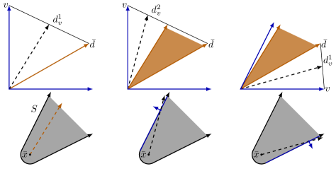
One iteration of Algorithm 2 for one direction $v$ is illustrated in Figure 2. The outer for loop in line 2 requires a V-representation of the polytope $\left\{{x\in\mathcal{O}\mid\left\lVert{x}\right\rVert_{\infty}\leq 1}\right\}$. During the execution of the algorithm, however, $\mathcal{O}$ is always given by an H-representation and $\mathcal{I}$ by a V-representation. Therefore, a vertex enumeration has to be performed in every iteration. The algorithm terminates if lines 2 - 2 are not executed during one full iteration, i.e. if $\mathcal{O}$ receives no upgrade. This happens only if for every $v$ of the set in line 2 and $k=\left\lceil\log_{2}\left(\frac{\left\lVert{v-d}\right\rVert}{\varepsilon}\right)\right\rceil$ the point $d_{v}^{k}$ belongs to $\mathcal{I}$. This implies

$$\inf_{d_{i}\in\mathcal{I}}\left\lVert{v-d_{i}}\right\rVert\leq\left\lVert{v-d_{v}^{k}}\right\rVert=\frac{1}{2^{k}}\left\lVert{v-\bar{d}}\right\rVert\leq\varepsilon$$

for every vertex $v$, which certifies $\bar{d}_{\mathsf{H}}(\mathcal{O},\mathcal{I})\leq\varepsilon$. Since $\mathcal{I}\subseteq\operatorname{0^{\infty}}S\subseteq\mathcal{O}$, the relations $\bar{d}_{\mathsf{H}}(\mathcal{O},\operatorname{0^{\infty}}S)\leq\varepsilon$ and $\bar{d}_{\mathsf{H}}(\operatorname{0^{\infty}}S,\mathcal{I})\leq\varepsilon$ follow. We now prove that Algorithm 2 works correctly and is finite.

Theorem 4.4.

Let Assumptions (S1)-(S3) be satisfied for a spectrahedral shadow $S$. Then Algorithm 2 terminates after finitely many steps and is correct, i.e. the algorithm returns an inner $\varepsilon$-approximation $\mathcal{I}$ and an outer $\varepsilon$-approximation $\mathcal{O}$ of $\operatorname{0^{\infty}}S$.

Proof.

We first prove the correctness. Assumptions (S1) and (S3) imply that $-\bar{d}\notin\operatorname{0^{\infty}}S$. Otherwise we had $0\in\operatorname{int}\operatorname{0^{\infty}}S$, which implies $S=\mathbb{R}^{n}$, see [47, Theorem 6.1]. Then, since $\mathcal{A}(\bar{x})+\mathcal{B}(\bar{y})+A\succ 0$ and $S$ is closed, a solution to (D₂($S,c,d$)) in line 1 exists according to Corollary 4.3. Furthermore, Assumption (S3) and Corollary 4.3 imply that the set $\mathcal{I}$ initialized in line 2 and the set $\mathcal{O}$ initialized in line 3 are an inner and an outer approximation of $\operatorname{0^{\infty}}S$, respectively. For the latter, take into account that the recession cone of a polyhedron in H-representation is described by the corresponding homogeneous system of inequalities, see [47, p. 62]. During the first execution of the outer for loop in lines 6–17, $\mathcal{O}=H^{-}(w^{*}/\left\lVert{w^{*}}\right\rVert,0)$ and the set $\left\{{x\in\mathcal{O}\mid\left\lVert x\right\rVert_{\infty}\leq 1}\right\}$ in line 2 is nonempty. In particular, it is a polytope and the for loop is executed at least once. Now, let $v$ be a from this set, for which the inner for loop is executed. Without loss of generality we can assume that such $v$ exists, otherwise we have

$$\log_{2}\left(\frac{\left\lVert{v-\bar{d}}\right\rVert}{\varepsilon}\right)\leq 0$$

for all vertices $v$ of $\left\{{x\in\mathcal{O}\mid\left\lVert x\right\rVert_{\infty}\leq 1}\right\}$. This implies that

$$\bar{d}_{\mathsf{H}}(\mathcal{O},\mathcal{I}) =\sup_{v\in\mathcal{O}\cap B}\inf_{d\in\mathcal{I}}\left\lVert{v-d}\right\rVert$$

$$\leq\sup_{v\in\mathcal{O}\cap\left\{{x\mid\left\lVert{x}\right\rVert_{\infty}\leq 1}\right\}}\inf_{d\in\mathcal{I}}\left\lVert{v-d}\right\rVert$$

$$\leq\max\left\{{\left\lVert{v-\bar{d}}\right\rVert\mid v\text{ is a vertex of }\mathcal{O}\cap\left\{{x\mid\left\lVert{x}\right\rVert_{\infty}\leq 1}\right\}}\right\}$$

$$\leq\varepsilon.$$

The first equality holds true because $\mathcal{I}\subseteq\mathcal{O}$ and the projection onto a convex cone is a norm-reducing operation, i.e. the infimum is attained for some $d\in B$, cf. [39]. The inequality in the second line simply reflects the fact that $B$ is contained in $\left\{{x\in\mathbb{R}^{n}\mid\left\lVert{x}\right\rVert_{\infty}\leq 1}\right\}$. Moreover, the supremum in the second line is attained at a vertex of $\mathcal{O}\cap\left\{{x\in\mathbb{R}^{n}\mid\left\lVert{x}\right\rVert_{\infty}\leq 1}\right\}$, see [4, Theorem 3.3]. Thus, $\mathcal{O}$ and $\mathcal{I}$ are $\varepsilon$-approximations of $\operatorname{0^{\infty}}S$ already.

Next, note that the search direction $d_{v}^{k}$ defined in line 8 is zero only if $v=-\bar{d}$. However, due to the fact that $\bar{x}\in\operatorname{int}\mathcal{S}$ it is straightforward to see, that the initial outer approximation in line 3 does not contain $-\bar{d}$. Hence, subsequent approximations also do not contain $-\bar{d}$, i.e. $d_{v}^{k}\neq 0$ for every vertex $v$ selected in line 2. Now, assume (P₂($S,c,d$)) is unbounded for some $k$, i.e. $\bar{x}+td_{v}^{k}\in S$ for every $t\geq 0$. Since $S$ is closed by Assumption (S1), this implies $d_{v}^{k}\in\operatorname{0^{\infty}}S$, see [47, Theorem 8.3]. Hence, the updated inner approximation in line 12 still satisfies $\mathcal{I}\subseteq\operatorname{0^{\infty}}S$. If (P₂($S,c,d$)) is not unbounded, then Assumption (S2) and Corollary 4.3 guarantee that (D₂($S,c,d$)) has an optimal solution $(U^{*},w^{*})$. Moreover, $H(w^{*},A\cdot U^{*})$ supports $S$, which implies that $H(w^{*}/\left\lVert{w^{*}}\right\rVert,0)$ supports $\operatorname{0^{\infty}}S$. Therefore, after the update in line 15 it still holds $\operatorname{0^{\infty}}S\subseteq\mathcal{O}$ and $\mathcal{O}$ is a cone.

It remains to show that upon termination of the algorihm, $\mathcal{I}$ and $\mathcal{O}$ are $\varepsilon$-approximations of $\operatorname{0^{\infty}}S$. Algorithm 2 terminates if and only if during one iteration of the repeat until loop in lines 4–18 the outer approximation is not modified, i.e. lines 14–17 are not executed. This is the case if and only if for vertex $v$ of $\left\{{x\in\mathcal{O}\mid\left\lVert{x}\right\rVert_{\infty}\leq 1}\right\}$ it holds $d_{v}^{\bar{k}(v)}\in\mathcal{I}$ with $\bar{k}(v)=\left\lceil\log_{2}\left(\frac{\left\lVert{v-d}\right\rVert}{\varepsilon}\right)\right\rceil$. Using the same derivation as above but replaing $\bar{d}$ with $d_{v}^{\bar{k}(v)}$ and taking into accound the relation

$$\left\lVert{v-d_{v}^{\bar{k}(v)}}\right\rVert \leq\left\lVert{v-\frac{\left\lVert{v-d}\right\rVert-\varepsilon}{\left\lVert{v-d}\right\rVert}v-\frac{\varepsilon}{\left\lVert{v-d}\right\rVert}d}\right\rVert$$

$$=\frac{\varepsilon}{\left\lVert{v-d}\right\rVert}\left\lVert{v-d}\right\rVert$$

$$=\varepsilon$$

this yields

$$\bar{d}_{\mathsf{H}}(\mathcal{O},\mathcal{I})\leq\varepsilon.$$

Since $\mathcal{I}\subseteq\operatorname{0^{\infty}}S\subseteq\mathcal{O}$ this implies both $\bar{d}_{\mathsf{H}}(\mathcal{O},\operatorname{0^{\infty}}S)\leq\varepsilon$ and $\bar{d}_{\mathsf{H}}(\operatorname{0^{\infty}}S,\mathcal{I})\leq\varepsilon$. This concludes the proof of correctness.

Now, we show that Algorithm 2 indeed terminates after finitely many iterations. Assume that at some point during the algorithm the approximations $\mathcal{O}$ and $\mathcal{I}$ have been computed and that the algorithm does not halt for these sets. Then there exists a vertex $v$ of the set in line 2 and some $k\leq\left\lceil\log_{2}\left(\frac{\left\lVert{v-\bar{d}}\right\rVert}{\varepsilon}\right)\right\rceil$ for which (P₂($S,c,d$)) is bounded. This implies that lines 14–17 are executed. Let ($U^{*},w^{*}$) be a solution to (D₂($S,c,d$)) and let $w$ be the normalized vector $w^{*}/\left\lVert{w^{*}}\right\rVert$. Then, by the same reasoning as above, the hyplerplane $H(w,0)$ supports $\operatorname{0^{\infty}}S$. Therefore, $\mathcal{I}\subseteq H^{-}(w,0)$. By Assumption (S3) there exists some $r>0$, such that $B_{r}(\bar{d}):=\left\{{x\in\mathbb{R}^{n}\mid\left\lVert{x-\bar{d}}\right\rVert\leq r}\right\}\subseteq\mathcal{I}$. Hence,

$$\inf\left\{{\left\lVert{x-d}\right\rVert\mid x\in H(w,0)}\right\} =\left\lvert w^{\mathsf{T}}d\right\rvert$$

$$=-w^{\mathsf{T}}d$$

$$\geq r.$$

Taking into account the definition of $d_{v}^{k}$ and the fact that $w^{*\mathsf{T}}d_{v}^{k}=1$, we conclude

$$\inf\left\{{\left\lVert{x-v}\right\rVert\mid x\in H(w,0)}\right\} =\left\lvert w^{\mathsf{T}}v\right\rvert$$

$$=w^{\mathsf{T}}v$$

$$\geq w^{\mathsf{T}}\left(\frac{2^{k}}{2^{k}-1}d_{v}^{k}-\frac{1}{2^{k}-1}\bar{d}\right)$$

$$=\frac{2^{k}}{(2^{k}-1)\left\lVert{w^{*}}\right\rVert}+\frac{r}{2^{k}-1}$$

$$\geq\frac{r}{2^{k}-1}$$

$$\geq\frac{r}{\frac{2\left\lVert{v-\bar{d}}\right\rVert}{\varepsilon}-1}$$

$$>\frac{\varepsilon r}{4\sqrt{n}-\varepsilon}.$$

The last inequality follows from $\left\lVert{v-\bar{d}}\right\rVert<2\sqrt{n}$. That means, whenever $\mathcal{O}$ receives an update in line 15, a ball of radius at least $\frac{\varepsilon r}{4\sqrt{n}-\varepsilon}$ around $v$ is cut off. Since $v$ belongs to the compact set $\left\{{x\in\mathbb{R}^{n}\mid\left\lVert{x}\right\rVert_{\infty}\leq 1}\right\}$, $\mathcal{O}$ can only be updated a finite number of times. This proves that the algorithm terminates. ∎

In comparison to Algorithm 1, the main advantage of Algorithm 2 is its higher degree of flexibility. It generalizes Algorithm 1 in two aspects. Firstly it works for spectrahedral shadows, which contain spectrahedra as a proper subclass, and secondly it is also applicable to sets with a recession cone that is not necessarily pointed. The only drawback of Algorithm 2 is that an interior point of the recession cone must be known beforehand and it is not trivial to compute one. However, knowledge of an interior point of the set to be approximated is a commom assumption in the literature about polyhedral approximation, see e.g. [26], where it is assumed, that the origin is contained in the interior of the set, [12], where some form of Slater’s constraint qualification is assumed, or [3], where some interior point is assumed to exist.

5 Examples

We apply Algorithms 1 and 2 to three examples in this section and provide numerical results. The algorithms are implemented in Python version 3.9.12. The semidefinite problems (P₁), (P₂) and (D₂) are solved using version 1.1.18 of the API CVXPY [11, 1] with the solver SCS [42]. To carry out the vertex and facet enumerations on the approximations we use the Python wrapper pycddlib of the library cddlib [16]. The figures in Examples 5.2 and 5.3 are generated with the polyhedral calculus toolbox bensolve tools [37, 10]. The first example considers a spectrahedron and is applied to both algorithms, while in Examples 5.2 and 5.3 spectrahedral shadows are investigated where only Algorithm 2 can be applied.

Example 5.1.

We consider the spectrahedron

$$C=\left\{{x\in\mathbb{R}^{3}\mid\begin{pmatrix}x_{1}&x_{2}\\ x_{2}&x_{3}\end{pmatrix}\succcurlyeq\begin{pmatrix}1&0\\ 0&1\end{pmatrix}}\right\}.$$

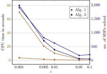
Its recession cone is the set $S_{+}^{2}$. As input parameters we set $\bar{x}=\frac{\sqrt{2}}{2}(1,0,1)^{\mathsf{T}}$ for Algorithm 1 and $\bar{x}=(2,0,2)^{\mathsf{T}}$, $\bar{d}=\frac{\sqrt{2}}{2}(1,0,1)^{\mathsf{T}}$ for Algorithm 2. Figure 3 shows the number of solved SDP subproblems and the elapsed CPU time for different values of $\varepsilon$ and both algorithms. We see that the number of solved subproblems is of the same order of magnitude for both algorithms. Hoewever, Algorithm 2 performs the approximation much faster, by a factor of around 23 for $\varepsilon=10^{-}3$. This is explained by the fact that the number of solved SDPs for Algorithm 2 includes the unbounded instances of (P₂($C,c,d$)), for which SCS can terminate as soon as the unboundedness is detected. Another remarkable observation is that the number of subproblems for Algorithm 1 is smaller for $\varepsilon=0.05$ than for $\varepsilon=0.1$. The reason is that the set $M$ approximated by Algorithm 1 depends on the value of $\varepsilon$. Recall that $M$ can be seen as a slice of $\operatorname{0^{\infty}}C$ and as $\varepsilon$ decreases so does the thickness of $M$. This evidently has an impact on the performance.

 

Figure 3: Computational results for Example 5.1.

Example 5.2.

We consider the cone $\Sigma_{1,4}$ of univariate polynomials of degree at most four which can be represented as a sum of squares of polynomials. By identifying the polynomials by their coefficients it can be written as the following spectrahedral shadow in $\mathbb{R}^{5}$:

$$\Sigma_{1,4}=\left\{{x\in\mathbb{R}^{5}\mid\exists y\in\mathbb{R}:\begin{pmatrix}x_{1}&\frac{1}{2}x_{2}&\frac{1}{3}x_{3}-y\\ \frac{1}{2}x_{2}&\frac{1}{3}x_{3}+2y&\frac{1}{2}x_{4}\\ \frac{1}{3}x_{3}-y&\frac{1}{2}x_{4}&x_{5}\end{pmatrix}\succcurlyeq 0}\right\}.$$

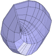
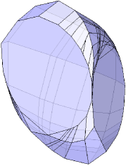
The cone of sums of squares of polynomials or SOS cone is contained in the cone of nonnegative polynomials. It is of interest, because optimization problems involving SOS polynomials are tractable by semidefinite programming [43]. For a derivation of semidefinite representations of SOS polynomials see [5, p. 61]. We approximate $\Sigma_{1,4}$ with $\varepsilon=0.1$ and $\bar{x}=\bar{d}=1/\sqrt{5}e$. Algorithm 2 computes the approximations in $26.4$ seconds while solving $1081$ subproblems. Figure 4 shows the projections of the base

$$\Sigma_{1,4}\cap\left\{{x\in\mathbb{R}^{5}\mid p^{\mathsf{T}}x=-1}\right\},$$

where $p\approx(-0.71,-0.08,-0.21,-0.08,-0.66)^{\mathsf{T}}$, onto the variables

$$\begin{pmatrix}x_{1}\\ x_{2}\\ x_{3}\end{pmatrix},\begin{pmatrix}x_{1}\\ x_{2}\\ x_{4}\end{pmatrix},\begin{pmatrix}x_{1}\\ x_{3}\\ x_{4}\end{pmatrix}\text{ and }\begin{pmatrix}x_{2}\\ x_{3}\\ x_{4}\end{pmatrix},$$

respectively.

 

Figure 4: The orthogonal projections of the 4-dimensional base of the cone $\Sigma_{1,4}$ from Example 5.2 onto three coordinates.

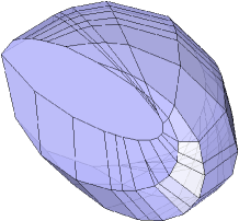
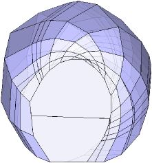
Example 5.3.

Since Algorithm 2 operates in the ambient space of the spectrahedral shadow and not in the space of the typically high dimensional spectrahedron, we want to investigate how well it scales with the size of the involved pencils. Therefore, we consider the shadow

$$S=\left\{{\begin{pmatrix}x_{11}\\ x_{22}\\ x_{33}\\ \ell(X)\end{pmatrix}\mid X\succcurlyeq I}\right\},$$

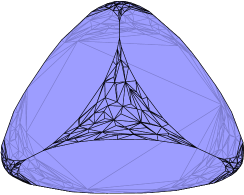
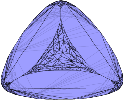
where $\ell(X)=x_{11}+x_{22}+x_{33}+2(x_{12}+x_{13}+x_{23})$, for different sizes $n$ of the matrix $X$. Since $X$ is symmetric the number of variables depends on $n$ as $\frac{n(n+1)}{2}$. For the computations we set $\bar{d}=(1,1,1,0)^{\mathsf{T}}$. Figure 5 shows the outer and inner approximations of the base

$$H\left(-\frac{1}{\sqrt{4}}e,-1\right)\cap\operatorname{0^{\infty}}{S}$$

for $n=3$ and $\varepsilon=0.01$, respectively. The set is the convex dual of a spectrahedron known as elliptope [38], which has applications in statistics. Some numerical results are presented in Table 1. It shows the size $n$ of the pencil, the numver of variables (#var), the number of solvex SDPs (#SDP) and the elapsed time. The number of solved SDPs for $\varepsilon=0.01$ is approximately the same for different $n$. For $n\geq 7$ the vertex enumeration fails and no results are obtainable. For $\varepsilon=0.1$ the computation time generally increases, although drops can be seen, for example for $n=9$. This may be explained by SCS taking advantage of the problem structure that is hidden from the user.

 

Figure 5: The outer and inner approximations of a base of $\operatorname{0^{\infty}}{S}$ computed by Algorithm 2, respectively.

$n$	#var	#SDP	time
3	6	474	2.25
6	21	673	12.92
9	45	384	6.10
12	78	673	23.84
15	120	721	45.96

$n$	#var	#SDP	time
3	6	11810	132.65
4	10	11879	111.39
5	15	11647	152.99
6	21	12059	308.07

Table 1: Numerical results for Example 5.3 for $\varepsilon=0.1$ and $\varepsilon=0.01$, respectively.

References

- [1] Akshay Agrawal, Robin Verschueren, Steven Diamond, and Stephen Boyd. A rewriting system for convex optimization problems. J. Control Decis., 5(1):42–60, 2018.
- [2] Charalambos D. Aliprantis and Rabee Tourky. Cones and duality, volume 84 of Graduate Studies in Mathematics. American Mathematical Society, Providence, RI, 2007.
- [3] Çağın Ararat, Firdevs Ulus, and Muhammad Umer. A norm minimization-based convex vector optimization algorithm, 2021.
- [4] R. G. Batson. Extensions of Radstrom’s lemma with application to stability theory of mathematical programming. J. Math. Anal. Appl., 117(2):441–448, 1986.
- [5] Grigoriy Blekherman, Pablo A. Parrilo, and Rekha R. Thomas, editors. Semidefinite optimization and convex algebraic geometry, volume 13 of MOS-SIAM Series on Optimization. Society for Industrial and Applied Mathematics (SIAM), Philadelphia, PA; Mathematical Optimization Society, Philadelphia, PA, 2013.
- [6] Stephen Boyd and Lieven Vandenberghe. Convex optimization. Cambridge University Press, Cambridge, 2004.
- [7] Lilian Button and John B. Wilker. Cutting exponents for polyhedral approximations to convex bodies. Geom. Dedicata, 7(4):415–426, 1978.
- [8] E. W. Cheney and A. A. Goldstein. Newton’s method for convex programming and Tchebycheff approximation. Numer. Math., 1:254–268, 1959.
- [9] Daniel Ciripoi. Approximation of spectrahedral shadows and spectralhedral calculus. dissertation, Friedrich Schiller University Jena, 2019.
- [10] Daniel Ciripoi, Andreas Löhne, and Benjamin Weißing. Calculus of convex polyhedra and polyhedral convex functions by utilizing a multiple objective linear programming solver. Optimization, 68(10):2039–2054, 2019.
- [11] Steven Diamond and Stephen Boyd. CVXPY: a Python-embedded modeling language for convex optimization. J. Mach. Learn. Res., 17:Paper No. 83, 5, 2016.
- [12] Marco A. Duran and Ignacio E. Grossmann. An outer-approximation algorithm for a class of mixed-integer nonlinear programs. Math. Programming, 36(3):307–339, 1986.
- [13] Daniel Dörfler, Andreas Löhne, Christopher Schneider, and Benjamin Weißing. A benson-type algorithm for bounded convex vector optimization problems with vertex selection. Optimization Methods and Software, 0(0):1–21, 2021.
- [14] Matthias Ehrgott, Lizhen Shao, and Anita Schöbel. An approximation algorithm for convex multi-objective programming problems. J. Global Optim., 50(3):397–416, 2011.
- [15] Gabriele Eichfelder. Variable ordering structures in vector optimization. Vector Optimization. Springer-Verlag Berlin Heidelberg, 2014.
- [16] Komei Fukuda and Alain Prodon. Double description method revisited. In Combinatorics and computer science (Brest, 1995), volume 1120 of Lecture Notes in Comput. Sci., pages 91–111. Springer, Berlin, 1996.
- [17] Christiane Gerstewitz. Nichtkonvexe Dualität in der Vektoroptimierung. Wiss. Z. Tech. Hochsch. Leuna-Merseburg, 25(3):357–364, 1983.
- [18] Christiane Gerth and Petra Weidner. Nonconvex separation theorems and some applications in vector optimization. J. Optim. Theory Appl., 67(2):297–320, 1990.
- [19] Rick Greer. Trees and Hills, volume 96 of North-Holland Mathematics Studies. North-Holland Publishing Co., Amsterdam, 1984.
- [20] Peter M. Gruber. Convex and discrete geometry, volume 336 of Grundlehren der mathematischen Wissenschaften [Fundamental Principles of Mathematical Sciences]. Springer, Berlin, 2007.
- [21] V. I. Gurariĭ. On inclinations of spaces and conditional bases in Banach space. Dokl. Akad. Nauk SSSR, 145:504–506, 1962.
- [22] Andreas H. Hamel. Translative sets and functions and their applications to risk measure theory and nonlinear separation. IMPA Report D21, Rio de Janeiro, 2006.
- [23] J. William Helton and Victor Vinnikov. Linear matrix inequality representation of sets. Comm. Pure Appl. Math., 60(5):654–674, 2007.
- [24] Frank Heyde and Andreas Löhne. Solution concepts in vector optimization: A fresh look at an old story. Optimization, 60(12):1421–1440, 2011.
- [25] Alfredo Iusem and Alberto Seeger. Distances between closed convex cones: old and new results. J. Convex Anal., 17(3-4):1033–1055, 2010.
- [26] G. K. Kamenev. A class of adaptive algorithms for the approximation of convex bodies by polyhedra. Zh. Vychisl. Mat. i Mat. Fiz., 32(1):136–152, 1992.
- [27] G. K. Kamenev. Efficiency of Hausdorff algorithms for polyhedral approximation of convex bodies. Zh. Vychisl. Mat. i Mat. Fiz., 33(5):796–805, 1993.
- [28] G. K. Kamenev. Investigation of an algorithm for the approximation of convex bodies. Zh. Vychisl. Mat. i Mat. Fiz., 34(4):608–616, 1994.
- [29] J. E. Kelley, Jr. The cutting-plane method for solving convex programs. J. Soc. Indust. Appl. Math., 8:703–712, 1960.
- [30] Lutz Kettner, Kurt Mehlhorn, Sylvain Pion, Stefan Schirra, and Chee Yap. Classroom examples of robustness problems in geometric computations. Comput. Geom., 40(1):61–78, 2008.
- [31] V. L. Klee, Jr. Extremal structure of convex sets. Arch. Math. (Basel), 8:234–240, 1957.
- [32] Jan Kronqvist, Andreas Lundell, and Tapio Westerlund. The extended supporting hyperplane algorithm for convex mixed-integer nonlinear programming. J. Global Optim., 64(2):249–272, 2016.
- [33] Catherine Lassez and Jean-Louis Lassez. Quantifier elimination for conjunctions of linear constraints via a convex hull algorithm. In Bruce Randall Donald, Deepak Kapur, and Joseph L. Mundy, editors, Symbolic and Numerical Computation for Artificial Intelligence. Academic Press, 1992.
- [34] Andreas Löhne. Vector Optimization with Infimum and Supremum. Vector optimization. Springer, Heidelberg, 2011.
- [35] Andreas Löhne. Approximate vertex enumeration, 2020.
- [36] Andreas Löhne, Birgit Rudloff, and Firdevs Ulus. Primal and dual approximation algorithms for convex vector optimization problems. J. Global Optim., 60(4):713–736, 2014.
- [37] Andreas Löhne and Benjamin Weiß ing. Equivalence between polyhedral projection, multiple objective linear programming and vector linear programming. Math. Methods Oper. Res., 84(2):411–426, 2016.
- [38] Mateusz Michał ek and Bernd Sturmfels. Invitation to nonlinear algebra, volume 211 of Graduate Studies in Mathematics. American Mathematical Society, Providence, RI, 2021.
- [39] J.-J. Moreau. Décomposition orthogonale d’un espace hilbertien selon deux cônes mutuellement polaires. C. R. Acad. Sci. Paris, 255:238–240, 1962.
- [40] Tim Netzer. Spectrahedra and their shadows. habilitation, University of Leipzig, 2011.
- [41] Peter E. Ney and Stephen M. Robinson. Polyhedral approximation of convex sets with an application to large deviation probability theory. J. Convex Anal., 2(1-2):229–240, 1995.
- [42] Brendan O’Donoghue, Eric Chu, Neal Parikh, and Stephen Boyd. SCS: Splitting conic solver, version 3.2.0. https://github.com/cvxgrp/scs, 2021.
- [43] Pablo A. Parrilo and Rekha R. Thomas. Sum of squares: theory and applications, volume 77 of Proceedings of Symposia in Applied Mathematics. American Mathematical Society, Providence, RI, 2020.
- [44] A. Pascoletti and P. Serafini. Scalarizing vector optimization problems. J. Optim. Theory Appl., 42(4):499–524, 1984.
- [45] Motakuri Ramana and A. J. Goldman. Some geometric results in semidefinite programming. J. Global Optim., 7(1):33–50, 1995.
- [46] Motakuri V. Ramana. An exact duality theory for semidefinite programming and its complexity implications. Math. Programming, 77(2, Ser. B):129–162, 1997.
- [47] R. Tyrrell Rockafellar. Convex Analysis. Princeton Mathematical Series, No. 28. Princeton University Press, Princeton, N.J., 1970.
- [48] R. Tyrrell Rockafellar and Roger J.-B. Wets. Variational analysis, volume 317 of Grundlehren der mathematischen Wissenschaften [Fundamental Principles of Mathematical Sciences]. Springer-Verlag, Berlin, 1998.
- [49] S. Ruzika and M. M. Wiecek. Approximation methods in multiobjective programming. J. Optim. Theory Appl., 126(3):473–501, 2005.
- [50] Claus Scheiderer. Semidefinite representation for convex hulls of real algebraic curves. SIAM J. Appl. Algebra Geom., 2(1):1–15, 2018.
- [51] Hoáng Tụy. On outer approximation methods for solving concave minimization problems. Acta Math. Vietnam., 8(2):3–34, 1983.
- [52] Tran Vu Thieu, Bui The Tam, and Vu Thien Ban. An outer approximation method for globally minimizing a concave function over a compact convex set. Acta Math. Vietnam., 8(1):21–40, 1983.
- [53] Arthur F. Veinott, Jr. The supporting hyperplane method for unimodal programming. Operations Res., 15:147–152, 1967.
- [54] Tapio Westerlund and Frank Pettersson. An extended cutting plane method for solving convex minlp problems. Comput. Chem. Eng., 19:131–136, 1995.