Randomized Coordinate Subgradient Method
for Nonsmooth Composite Optimization

Abstract

Coordinate-type subgradient methods for addressing nonsmooth optimization problems are relatively underexplored due to the set-valued nature of the subdifferential. In this work, our study focuses on nonsmooth composite optimization problems, encompassing a wide class of convex and weakly convex (nonconvex nonsmooth) problems. By utilizing the chain rule of the composite structure properly, we introduce the Randomized Coordinate Subgradient method (RCS) for tackling this problem class. To the best of our knowledge, this is the first coordinate subgradient method for solving general nonsmooth composite optimization problems. In theory, we consider the linearly bounded subgradients assumption for the objective function, which is more general than the traditional Lipschitz continuity assumption, to account for practical scenarios. We then conduct convergence analysis for RCS in both convex and weakly convex cases based on this generalized Lipschitz-type assumption. Specifically, we establish the $\widetilde{\mathcal{O}}(1/\sqrt{k})$ convergence rate in expectation and the $\tilde{o}(1/\sqrt{k})$ almost sure asymptotic convergence rate in terms of the suboptimality gap when $f$ is convex, where $k$ represents iteration count. If $f$ further satisfies the global quadratic growth condition, the improved $\mathcal{O}(1/k)$ rate is derived in terms of the squared distance to the optimal solution set. For the case when $f$ is weakly convex and its subdifferential satisfies the global metric subregularity property, we derive the $\mathcal{O}(\varepsilon^{-4})$ iteration complexity in expectation, where $\varepsilon$ is the target accuracy. We also establish an asymptotic convergence result. To justify the global metric subregularity property utilized in the analysis, we establish this error bound condition for the concrete (real-valued) robust phase retrieval problem. We also provide a convergence lemma and the relationship between the global metric subregularity properties of a weakly convex function and its Moreau envelope. These results are of independent interest. Finally, we conduct several experiments to demonstrate the possible superiority of RCS over the subgradient method.

1 Introduction

Coordinate-type methods tackle optimization problems by successively solving simpler (even scalar) subproblems along coordinate directions. These methods are widely used in signal processing, machine learning, and other engineering fields due to their simplicity and efficiency, see, e.g., [1, 2, 3, 4]. Coordinate methods are particularly useful when the problem size (measured as the dimension of the variable) is enormous and the computation of function values or full gradients can exhaust memory, or when the problem data is incrementally received or distributed across a network, requiring computation with whatever data is currently available. For more motivational statements, we refer to [1, 5, 6].

1.1 Motivations, problem setup, and examples

Existing works in this field mainly focus on extending gradient-based methods (e.g., the gradient descent, proximal gradient descent, and primal-dual methods) to coordinate methods; see, e.g., [5, 7, 8, 6, 1, 9, 10] and the references therein. In contrast, a parallel line of research on implementing a coordinate-type extension for the subgradient oracle is relatively unexplored and the related works in this line are surprisingly limited (to the best of our knowledge). The primary challenge in designing a coordinate-type subgradient method for general nonsmooth optimization problems stems from the set-valued nature of the subdifferential. Specifically, the Cartesian product of coordinate-wise subgradients may not necessarily give rise to a complete subgradient, rendering the convergence of such a method unclear in both practical implementation and theoretical analysis. Despite this general difficulty, our goal is to design a coordinate-type subgradient method for a class of structured nonsmooth optimization problems.

In this work, we consider the composite optimization problem

$$\min_{x\in\mathbb{R}^{d}}\ f(x)=h(\Phi(x)),$$ (1)

where the outer function $h:\mathbb{R}^{n}\to\mathbb{R}$ is possibly nonsmooth and the inner function $\Phi:\mathbb{R}^{d}\to\mathbb{R}^{n}$ is a smooth mapping. In addition, the objective function $f:\mathbb{R}^{d}\to\mathbb{R}$ is $\rho$-weakly convex (i.e., $f+\frac{\rho}{2}\|\cdot\|^{2}$ is convex for some $\rho\geq 0$). When $\rho=0$, $f$ reduces to a convex function.

The composite form (1) is a common source of nonsmooth convex and weakly convex functions; see, e.g., [11, 12, 13]. It covers many signal processing and machine learning problems as special instances. We list three of them below. One can easily put the three examples into the composite form (1), while the weak convexity of $f$ in these examples comes from one of the following two cases:

1. The outer function $h$ is convex and $L_{h}$-Lipschitz continuous and the derivative of the inner smooth mapping $\Phi$ (presented by the $n\times d$ Jacobian matrix $\nabla\Phi$) is $L_{\Phi}$-Lipschitz continuous. In this case, $f$ is $L_{h}L_{\Phi}$-weakly convex according to [14, Lemma 4.2].

2. The outer function $h$ is $\rho_{h}$-weakly convex and $L_{h}$-Lipschitz continuous and the inner smooth mapping $\Phi$ is $L_{\Phi}^{0}$-Lipschitz continuous and its Jacobian $\nabla\Phi$ is $L_{\Phi}$-Lipschitz continuous. In this case, we can establish that $f$ is $\left(\rho_{h}(L_{\Phi}^{0})^{2}+L_{h}L_{\Phi}\right)$-weakly convex; see Lemma 2.1.

Application 1: Robust M-estimators. The robust M-estimator problem is defined as [15]:

$$\min_{x\in\mathbb{R}^{d}}\ f(x):=\ell(Ax-b)+\sum_{i=1}^{d}\phi_{p}(x_{i}),$$ (2)

where $A\in\mathbb{R}^{n\times d}$ is a matrix, $b\in\mathbb{R}^{n}$ is a vector, $\ell$ is a Lipschitz continuous loss function like $\ell_{1}$-norm, MCP [16] and SCAD [17], and $\phi_{p}$ is a Lipschitz continuous penalty function such as $\ell_{1}$-norm, MCP, SCAD, etc. In this problem, let us define $\Phi:\mathbb{R}^{d}\to\mathbb{R}^{n}\times\mathbb{R}^{d}$ by $\Phi(x)=\left(Ax-b,x\right)$ and $h:\mathbb{R}^{n}\times\mathbb{R}^{d}\rightarrow\mathbb{R}$ by $h(y,z)=\ell(y)+\sum_{i=1}^{d}\phi_{p}(z_{i})$. Then, the weak convexity of $f$ follows from the case (C.2). In this way, we have placed problem (2) in the composite form (1).

Application 2: SVM. Support vector machine (SVM) is a popular supervised learning method, which is widely used for classification. The linear SVM problem can be expressed as [18, 19]

$$\min_{x\in\mathbb{R}^{d}}\ f(x):=\frac{1}{n}\sum_{i=1}^{n}\max\left\{0,1-b_{i}(a_{i}^{\top}x)\right\}+\frac{p}{2}\|x\|^{2},$$ (3)

where $p>0$, $a_{i}\in\mathbb{R}^{d}$, and $b_{i}\in\{\pm 1\}$, $i=1,...,n$. Let $A=\left(a_{1}^{\top},...,a_{n}^{\top}\right)\in\mathbb{R}^{n\times d}$, $b=\left(b_{1},...,b_{n}\right)\in\mathbb{R}^{n}$, $\mathbb{R}^{n\times d}\ni\tilde{A}=\mathrm{diag}(b)A$, and $1_{n}$ be a $n$-dimensional vector of all $1$s. We define $\Phi:\mathbb{R}^{d}\to\mathbb{R}^{n}\times\mathbb{R}$ by $\Phi(x)=(1_{n}-\tilde{A}x,\frac{p}{2}\|x\|^{2})$ and $h:\mathbb{R}^{n}\times\mathbb{R}\to\mathbb{R}$ by $h(y,z)=\frac{1}{n}\sum_{i=1}^{n}\max\{0,y_{i}\}+z$. Furthermore, the weak convexity of $f$ follows from the fact that the problem is even convex (i.e., $\rho=0$). Then, one can see that problem (3) has the composite form (1).

Application 3: (Real-valued) Robust phase retrieval problem. Phase retrieval is a common computational problem with applications in diverse areas such as physics, imaging science, X-ray crystallography, and signal processing [20]. The (real-valued) robust phase retrieval problem amounts to solving [21]

$$\min_{x\in\mathbb{R}^{d}}\ f(x):=\frac{1}{n}\|(Ax)^{\circ 2}-b^{\circ 2}\|_{1},$$ (4)

where $A\in\mathbb{R}^{n\times d}$, $b\in\mathbb{R}^{n}$, and $\circ 2$ is the Hadamard power. It is obvious that problem (4) has the composite form in (1) by setting $\Phi(x)=(Ax)^{\circ 2}-b^{\circ 2}$ and $h(\cdot)=\frac{1}{n}\|\cdot\|_{1}$ and realizing that $f$ is weakly convex due to the case (C.1).

It is interesting to observe that $f$ in problem (2) is Lipschitz continuous but can be weakly convex due to SCAD and MCP loss function or penalty. $f$ in problem (3) is convex. However, it is not Lipschitz continuous due to the weight decay term $\|x\|^{2}$. $f$ in problem (4) is simultaneously weakly convex and non-Lipschitz continuous. In this work, we aim at designing a coordinate-type subgradient method for solving the nonsmooth composite optimization problem (1). Then, we derive its convergence theory, which covers the weakly convex and/or non-Lipschitz problems such as Applications 1–3.

1.2 Main contributions

Our main contributions are summarized as follows.

1. Despite the fundamental bottleneck of designing a coordinate-type subgradient method for general nonsmooth optimization problems, we focus on the structured composite problem (1). The key insight lies in that this composite structure admits the chain rule subdifferential calculus, which allows to separate the derivative of the smooth mapping $\Phi$ and the subdifferential of the outer nonsmooth function $h$. Consequently, such a structured subdifferential presents a natural coordinate separation. Based on this insight, we design a Randomized Coordinate Subgradient method (RCS) (see Algorithm 1) for solving problem (1). To our knowledge, RCS is the first coordinate-type subgradient method for tackling general nonsmooth composite optimization problems.

2. Motivated by our examples that the traditional Lipschitz continuity assumption on the objective function $f$ can be stringent, we employ the more general linearly bounded subgradients assumption (see 2.1) in our analysis. When $f$ is convex (i.e., $\rho=0$) and under the linearly bounded subgradients assumption: $\bullet$) We derive the $\widetilde{\mathcal{O}}(1/\sqrt{k})$ convergence rate in expectation in terms of the suboptimality gap (see Theorem 5.1). $\bullet$) We show $\mathcal{O}(1/k)$ convergence rate in expectation with respect to the squared distance between the iterate and the optimal solution set under an additional global quadratic growth condition (see Theorem 5.2). $\bullet$) We establish the almost sure asymptotic convergence result (see Theorem 5.3) and the almost sure $\tilde{o}(1/\sqrt{k})$ asymptotic convergence rate result (see Corollary 5.1) in terms of the suboptimality gap, which are valid for each single run of RCS with probability 1. One important step for deriving these convergence results is to establish the boundedness of the iterates in expectation so that the technical difficulty introduced by the more general linearly bounded subgradients assumption can be tackled by using diminishing step sizes. We refer to Section 5 for more details.

3. When $f$ is weakly convex (i.e., $\rho>0$) and under the linearly bounded subgradients assumption: $\bullet$) We provide the iteration complexity of $\mathcal{O}(\varepsilon^{-4})$ in expectation for driving the Moreau envelope gradient below $\varepsilon$ (see Theorem 6.1). $\bullet$) We derive the almost sure asymptotic convergence result (see Theorem 6.2) and the almost sure $\mathcal{O}(1/k^{-\frac{1}{4}})$ asymptotic convergence rate result (in the sense of liminf; see Corollary 6.1) in terms of the Moreau envelope gradient. Our analysis for weakly convex case deviates from the standard one [13] due to the more general 2.1. Our key idea is to utilize an error bound condition (the global metric subregularity) to derive the approximate descent property of RCS (see Lemma 6.1). Towards establishing the desired results, we derive a convergence lemma for mapping (see Lemma 4.1) and the relationship between the global metric subregularity properties of a weakly convex function and its Moreau envelope (see Corollary 4.1), which are of independent interests.

4. We establish that the (real-valued) robust phase retrieval problem (4) satisfies the global metric subregularity property under a mild condition (see Proposition 4.1). This finding validates the key assumption we utilized for analyzing RCS in the weakly convex case for this specific problem. This established error bound condition is expected to be useful for analyzing other robust phase retrieval algorithms.

Finally, we remark that if we set the number of blocks $N=1$ in RCS, i.e., the algorithm reduces to the subgradient method, the above convergence results yield new results for the subgradient method under the linearly bounded subgradients assumption.

1.3 Related works

The coordinate-type subgradient methods. To the best of our knowledge, the exploration of extending the subgradient oracle into the coordinate regime remains relatively underexplored due to the set-valued nature of the subdifferential. In [22], Nesterov proposed a randomized coordinate extension of the subgradient method for solving convex linear composite optimization problems. The convex linear composition structure is a special instance of our problem (1). The reported convergence rate result was achieved using the impractical Polyak’s step size rule. The incorporation of randomization is crucial for connecting the analysis of their algorithm with the traditional subgradient method. The work [23] follows the same randomization idea and establishes a similar convergence rate result for their coordinate-type subgradient method applied to general nonsmooth convex optimization problems. However, their algorithm needs to calculate the full subgradient at each iteration, and then randomly select one block of the calculated subgradient for the coordinate update, in order to avoid the intrinsic obstacle induced by the set-valued nature of the subdifferential; see the last paragraph of [23, Section 1]. This approach negates the inherent advantage of coordinate-type methods over their full counterparts. In theory, the results in [22, 23] only apply to convex and Lipschitz continuous optimization problems. Unfortunately, this limitation excludes our three examples outlined in Subsection 1.1. By contrast, 1) our proposed RCS applies to the more general composite problem class (1) and 2) our theoretical findings extend to non-Lipschitz and weakly convex cases.

Analysis under generalized Lipschitz-type assumptions. The linearly bounded subgradients assumption dates back to [24], in which Cohen and Zhu showed the global convergence of the subgradient method for nonsmooth convex optimization. This assumption was later imposed in [25] to analyze stochastic subgradient method for stochastic convex optimization. However, both works concern the global convergence property while no explicit rate result is reported.

Apart from the assumption we used, there are several other directions for generalizing the theory of subgradient-type methods to non-Lipschitz convex optimization. In [26], the author proposed the concept of relative continuity of the objective function, which is to impose some relaxed bound on the subgradients by using Bregman distance. Then, the author invoked this Bregman distance in the algorithmic design. The resultant mirror descent-type algorithm has a different structure from the classic subgradient method. Similar idea was later used in [27] for analyzing online convex optimization problem. The works [28, 29] transform the original non-Lipschitz objective function to a radial reformulation, which introduces a new decision variable. Then, their algorithms are based on alternatively updating the original variable (by a subgradient step) and the new variable. In [30], a growth condition rather than Lipschitz continuity of $f$ was utilized to analyze the normalized subgradient method. The author obtained asymptotic convergence rate result in terms of the minimum of the suboptimality gap through a rather quick argument that originates in Shor’s analysis [31, Theorem 2.1]. This convergence result finally applies to any convex function that only needs to be locally Lipschitz continuous.

The common feature of the above mentioned works lies in that they all consider convex optimization problems. By contrast, our work studies both convex and nonconvex cases.

1.4 Notation

The notation in this paper is mostly standard. Throughout this work, we use $\mathbb{X}^{*}$ to denote the set of optimal solutions of (1). We assume $\mathbb{X}^{*}\neq\emptyset$ without loss of generality. For any $x^{*}\in\mathbb{X}^{*}$, we denote $f^{*}=f(x^{*})$. If problem (1) is nonconvex, the set of its critical points is denoted by $\overline{\mathbb{X}}$. Note that the indices $i(k)$, $k=0,1,2,\ldots$ generated in RCS are random variables. Thus, RCS generates a stochastic process $\{x^{k}\}_{k\geq 0}$. Throughout this work, let $(\Omega,\mathcal{F},\{\mathcal{F}_{k}\}_{k\geq 0},\mathbb{P})$ be a filtered probability space and let us assume that the sequence of iterates $\{x^{k}\}_{k\geq 0}$ is adapted to the filtration $\{\mathcal{F}_{k}\}_{k\geq 0}$, i.e., each of the random vectors $x^{k}:\Omega\to\mathbb{R}^{d}$ is $\mathcal{F}_{k}$-measurable, which is automatically true once we set $\mathcal{F}_{k}=\sigma(i(0),i(1),\ldots,i(k))$. We use $\mathbb{E}_{i(k)}$ and $\mathbb{E}_{\mathcal{F}_{k}}$ to denote the expectations taken over the random variable $i(k)$ and the filtration $\mathcal{F}_{k}$, respectively. We $\widetilde{\mathcal{O}}$ and $\tilde{o}$ to denote $\mathcal{O}$ and $o$ with hidden log terms, respectively.

2 Preliminaries and A Generalized Lipschitz-type Assumption

2.1 Convexity, weak convexity, and subdifferential

For a convex function $\psi:\mathbb{R}^{d}\rightarrow\mathbb{R}$, a vector $v\in\mathbb{R}^{d}$ is called a subgradient of $\psi$ at point $x$ if the subgradient inequality $\psi(y)\geq\psi(x)+\langle v,y-x\rangle$ holds for all $y\in\mathbb{R}^{d}$. The set of all subgradients of $\psi$ at $x$ is called the subdifferential of $\psi$ at $x$, denoted by $\partial\psi(x)$.

A function $\varphi:\mathbb{R}^{d}\rightarrow\mathbb{R}$ is $\rho$-weakly convex if $\psi=\varphi+\frac{\rho}{2}\|\cdot\|^{2}$ is convex. For such a $\rho$-weakly convex function $\varphi$, its subdifferential is given by [32, Proposition 4.6]

$$\partial\varphi(x)=\partial\psi(x)-\rho x,$$

where $\partial\psi$ is the convex subdifferential defined above. Additionally, it is well known that the $\rho$-weak convexity of $\varphi$ is equivalent to [32, Proposition 4.8]

$$\varphi(y)\geq\varphi(x)+\langle\nu,y-x\rangle-\frac{\rho}{2}\|x-y\|^{2}$$ (5)

for all $x,y\in\mathbb{R}^{d}$ and $\nu\in\partial\varphi(x)$.

In the following lemma, we establish that the composite case (C.2) gives rise to the weak convexity of $f$.

Lemma 2.1.

Suppose that the function $h:\mathbb{R}^{n}\rightarrow\mathbb{R}$ is $\rho_{h}$-weakly convex and $L_{h}$-Lipschitz continuous and the mapping $\Phi:\mathbb{R}^{d}\rightarrow\mathbb{R}^{n}$ is smooth, $L_{\Phi}^{0}$-Lipschitz continuous, and its Jacobian $\nabla\Phi$ is $L_{\Phi}$-Lipschitz continuous. Then, the composite function $f(x)=h(\Phi(x))$ is $\left(\rho_{h}(L_{\Phi}^{0})^{2}+L_{h}L_{\Phi}\right)$-weakly convex.

Proof.

For any $\zeta\in\partial h(\Phi(x))$, by the $\rho_{h}$-weak convexity of $h$ and (5), we have

$$h(\Phi(y))-h(\Phi(x)) \geq\langle\zeta,\Phi(y)-\Phi(x)\rangle-\frac{\rho_{h}}{2}\|\Phi(x)-\Phi(y)\|^{2}$$ (6)

$$\geq\langle\nabla\Phi(x)^{\top}\zeta,y-x\rangle-\frac{\rho_{h}}{2}\|\Phi(x)-\Phi(y)\|^{2}+\langle\zeta,\Phi(y)-\Phi(x)-\nabla\Phi(x)(y-x)\rangle$$

$$\geq\langle\nabla\Phi(x)^{\top}\zeta,y-x\rangle-\frac{\rho_{h}}{2}\|\Phi(x)-\Phi(y)\|^{2}-\|\zeta\|\cdot\|\Phi(y)-\Phi(x)-\nabla\Phi(x)(y-x)\|.$$

Since the Jacobian $\nabla\Phi$ is $L_{\Phi}$-Lipschitz continuous, we have that $\|\Phi(y)-\Phi(x)-\nabla\Phi(x)(y-x)\|\leq\frac{L_{\Phi}}{2}\|x-y\|^{2}$. By the $L_{\Phi}^{0}$-Lipschitz of $\Phi$, we obtain that $\|\Phi(x)-\Phi(y)\|^{2}\leq(L_{\Phi}^{0})^{2}\|x-y\|^{2}$. By the $L_{h}$-Lipschitz of $h$, we obtain that $\|\zeta\|\leq L_{h}$. Finally, invoking these bounds into (6) gives

$$h(\Phi(y))\geq h(\Phi(x))+\langle\nabla\Phi(x)^{\top}\zeta,y-x\rangle-\frac{\rho_{h}(L_{\Phi}^{0})^{2}+L_{h}L_{\Phi}}{2}\|x-y\|^{2},$$

which yields the desired result. ∎

2.2 Moreau envelope of weakly convex function

If $f$ is $\rho$-weakly convex, proper, and lower semicontinuous, then the Moreau envelope function $f_{\lambda}(x)$ and the proximal mapping $prox_{\lambda,f}(x)$ are defined as [33]:

$$f_{\lambda}(x):=\min_{y}\left\{f(y)+\frac{1}{2\lambda}\|y-x\|^{2}\right\},$$ (7)

$$prox_{\lambda,f}(x):=\arg\min_{y}\left\{f(y)+\frac{1}{2\lambda}\|y-x\|^{2}\right\}.$$ (8)

As a standard requirement on the regularization parameter $\lambda$, we will always use $\lambda<\frac{1}{\rho}$ in the sequel to ensure that $\nabla f_{\lambda}$ of a $\rho$-weakly convex function $f$ is well defined.

We collect a series of important and known properties of the Moreau envelope in the following proposition; see, e.g., [34, Propositions 1-4].

Proposition 2.1.

Suppose that $f$ is a $\rho$-weakly convex function. The following assertions hold:

1. $prox_{\lambda,f}(x)$ is well defined, single-valued, and Lipschitz continuous.

2. $f_{\lambda}(x)\leq f(x)-\frac{1-\lambda\rho}{2\lambda}\|x-prox_{\lambda,f}(x)\|^{2}$.

3. $\lambda\operatorname{dist}(0,\partial f(prox_{\lambda,f}(x)))\leq\|x-prox_{\lambda,f}(x)\|\leq\frac{\lambda}{1-\lambda\rho}\operatorname{dist}(0,\partial f(x))$.

4. $\nabla f_{\lambda}(x)=\frac{1}{\lambda}(x-prox_{\lambda,f}(x))$ and it is Lipschitz continuous.

5. $x=prox_{\lambda,f}(x)$ if and only if $0\in\partial f(x)$.

We have the following corollaries of Proposition 2.1, which show that the weakly convex function and its Moreau envelope mapping have the same set of optimal solutions and stationary points.

Corollary 2.1.

Suppose that $f$ is a $\rho$-weakly convex function. Let $\mathbb{X}_{\lambda}^{*}$ denote the set of minimizers of the problem $\min_{x\in\mathbb{R}^{d}}f_{\lambda}(x)$. Then, the following statements hold:

1. $f_{\lambda}(x)\geq f^{*}$ for all $x\in\mathbb{R}^{d}$.

2. $f_{\lambda}(x_{\lambda}^{*})=f^{*}$ for all $x_{\lambda}^{*}\in\mathbb{X}_{\lambda}^{*}$. Consequently, we have $\mathbb{X}_{\lambda}^{*}=\mathbb{X}^{*}$.

Proof.

We first show part (a). By the definition of $f_{\lambda}(x)$, we have

$$f_{\lambda}(x)=\min_{y\in\mathbb{R}^{d}}\left\{f(y)+\frac{\|x-y\|^{2}}{2\lambda}\right\}=f(prox_{\lambda,f}(x))+\frac{\|x-prox_{\lambda,f}(x)\|^{2}}{2\lambda}\geq f(prox_{\lambda,f}(x))\geq f^{*}.$$

We now show part (b). By argument (b) of Proposition 2.1, we have for all $x^{*}\in\mathbb{X}^{*}$ and $x_{\lambda}^{*}\in\mathbb{X}_{\lambda}^{*}$ that

$$f^{*}=f(x^{*})\geq f_{\lambda}(x^{*})\geq f_{\lambda}(x_{\lambda}^{*})\geq f^{*},$$

where the first inequality follows from argument (b) of Proposition 2.1 and the last inequality is due to part (a) of this corollary. The above inequality yields that $f^{*}=f(x^{*})=f_{\lambda}(x_{\lambda}^{*})$ for all $x^{*}\in\mathbb{X}^{*}$ and $x_{\lambda}^{*}\in\mathbb{X}_{\lambda}^{*}$. Thus, we have $\mathbb{X}^{*}=\mathbb{X}_{\lambda}^{*}$. ∎

Corollary 2.2.

Suppose that $f$ is a $\rho$-weakly convex function. Let $\overline{\mathbb{X}}_{\lambda}$ be the set of critical points of the problem $\min_{x\in\mathbb{R}^{d}}f_{\lambda}(x)$. Then, we have $\overline{\mathbb{X}}=\overline{\mathbb{X}}_{\lambda}$.

Proof.

This corollary is a direct consequence of parts (c) and (d) of Proposition 2.1. ∎

2.3 The supermartingale convergence theorem

Next, we introduce a well known convergence theorem in stochastic optimization society.

Theorem 2.1 (Supermartingale convergence theorem [35]).

Let $\{\Lambda^{k}\}_{k\in\mathbb{N}}$, $\{\mu^{k}\}_{k\in\mathbb{N}}$, $\{\nu^{k}\}_{k\in\mathbb{N}}$, and $\{\eta^{k}\}_{k\in\mathbb{N}}$ be four positive sequences of real-valued random variables adapted to the filtration $\{\xi_{k}\}_{k\in\mathbb{N}}$. Suppose the following recursion holds true:

$$\mathbb{E}_{\xi_{k}}\left[\Lambda^{k+1}\right]\leq(1+\mu^{k})\Lambda^{k}+\nu^{k}-\eta^{k},\quad\forall\ k\in\mathbb{N},$$

where

$$\sum_{k\in\mathbb{N}}\mu^{k}<\infty\quad\mbox{and}\quad\sum_{k\in\mathbb{N}}\nu^{k}<\infty\quad\mbox{almost surely}.$$

Then, the sequence $\{\Lambda^{k}\}_{k\in\mathbb{N}}$ almost surely converges to a finite random variable $\bar{\Lambda}$ and $\sum_{k\in\mathbb{N}}\eta^{k}<\infty$ almost surely.

2.4 The linearly bounded subgradients assumption

Let us present a more general condition than the traditional Lipschitz continuity assumption in this subsection. A fundamental result in variational analysis and nonsmooth optimization is the equivalence between Lipschitz continuity and bounded subgradients for a very general class of functions [33, Theorem 9.13]. Thus, in order to generalize the Lipschitz continuity or bounded subgradients assumption (they are equivalent as outlined), we impose the following linearly bounded subgradients assumption.

Assumption 2.1.

There exist constants $L_{1}\geq 0$, $L_{2}>0$ such that the function $f$ in (1) satisfies

$$\|r\|\leq L_{1}\|x\|+L_{2},\quad\forall x\in\mathrm{dom\\ }(f),\ \ r\in\partial f(x).$$

When $L_{1}=0$, 2.1 reduces to the traditional Lipschitz continuity assumption, i.e., $f$ is $L_{1}$-Lipschitz continuous [33, Theorem 9.13]. Nonetheless, it is significantly more general with $L_{1}>0$. For instance, problem (3) satisfies our assumption trivially due to the linearly bounded term $L_{1}\|x\|$. Moreover, considerably many weakly convex problems satisfy our assumption. By checking the subdifferential, it is easy to verify that our assumption holds for problem (4) (see Proposition 4.1 for its subdifferential) and the robust low-rank matrix recovery problem [36]. Indeed, the composite form $h(\Phi(x))$ in (1) with $h$ being $L_{h}$-Lipschitz continuous and the map $\Phi$ having $L_{\Phi}$-Lipschitz continuous Jacobian satisfies our assumption. Note that $\nabla\Phi(x)^{\top}\zeta\in\partial f(x)$ for any $\zeta\in\partial h(\Phi(x))$ according to (9). Then, it is easy to see that $\|\nabla\Phi(x)^{\top}\zeta\|\leq L_{h}\|\nabla\Phi(x)\|\leq L_{h}\|\nabla\Phi(x)-\nabla\Phi(0)\|+\|\nabla\Phi(0)\|\leq L_{h}L_{\Phi}\|x\|+\|\nabla\Phi(0)\|$. Since $\nabla\Phi(x)$ is continuous, there exists a $L_{2}>0$ such that $\|\nabla\Phi(0)\|\leq L_{2}$, which, together with defining $L_{1}=L_{h}L_{\Phi}$, establishes the claim.

3 Randomized Coordinate Subgradient Method

In this section, we introduce a coordinate-type subgradient method for solving problem (1). The convexity / weak convexity of $f$ is currently not required in algorithm design. We first reveal a structured property of the subdifferential of the composite objective function $f$ in (1). According to the composite structure, its subdifferential is given by [33, Theorem 10.6]

$$\boxed{\quad\partial f(x)=\nabla\Phi(x)^{\top}\partial h(\Phi(x))\quad}$$ (9)

where $\nabla\Phi(x)\in\mathbb{R}^{n\times d}$ is the Jacobian of the smooth map $\Phi$ at $x$ and $\partial h(\Phi(x))$ is the subdifferential of the outer function $h$ at $\Phi(x)$. For any subgradient $\zeta\in\partial h(\Phi(x))$, we have $\zeta\in\mathbb{R}^{n}$.

One important feature of $\partial f(x)$ is that it enables block coordinate computation as it fully separates the smooth part $\nabla\Phi(x)$ and the nonsmooth part $\partial h(\Phi(x))$. Let us decompose $\mathbb{R}^{d}$ into $N$ subspaces $\mathbb{R}^{d}=\bigotimes_{i=1}^{N}\mathbb{R}^{d_{i}}$ with $d=\sum_{i=1}^{N}d_{i}$. Correspondingly, the decision variable $x\in\mathbb{R}^{d}$ is decomposed into $N$ block coordinates $x=(x_{1},\ldots,x_{i},\ldots,x_{N})$ with $x_{i}\in\mathbb{R}^{d_{i}}$ and the Jacobian $\nabla\Phi(x)$ is decomposed into $N$ column-wise blocks

$$\nabla\Phi(x)=\begin{bmatrix}\nabla_{1}\Phi(x),\ldots,\nabla_{i}\Phi(x),\ldots,\nabla_{N}\Phi(x)\end{bmatrix}$$

where $\nabla_{i}\Phi(x)\in\mathbb{R}^{n\times d_{i}}$ represents the derivative of $\Phi$ with respective to the block coordinate $x_{i}\in\mathbb{R}^{d_{i}}$. To compute the $i$-th block coordinate subgradient of the objective function $f$, i.e., the subgradient of $f$ with respect to the block coordinate $x_{i}\in\mathbb{R}^{d_{i}}$, we can follow the two steps:

1. Compute a subgradient $\zeta\in\partial h(\Phi(x))$ of the outer function $h$ at $\Phi(x)$.

2. Compute the block coordinate Jacobian $\nabla_{i}\Phi(x)\in\mathbb{R}^{n\times d_{i}}$ and then compute the $i$-th block coordinate subgradient $r_{i}$ of $f$ by $r_{i}=\nabla_{i}\Phi(x)^{\top}\zeta\in\mathbb{R}^{d_{i}}$.

In this way, aggregating all the $N$ block coordinate subgradients results in a complete subgradient of $f$, i.e.,

$$\mathbb{R}^{d}\ni r:=\begin{bmatrix}r_{1}\\ \vdots\\ r_{N}\end{bmatrix}=\left[\begin{array}[]{c}\nabla_{1}\Phi(x)^{\top}\zeta\\ \vdots\\ \nabla_{N}\Phi(x)^{\top}\zeta\end{array}\right]\in\partial f(x).$$ (10)

The key factor of the above development lies in that one can pre-compute and then fix the subgradient $\zeta$ of the nonsmooth part, while the block coordinate separation is achieved by separating the Jacobian of the smooth part $\nabla\Phi(x)$, which is well defined.

Now, we are ready to design the Randomized Coordinate Subgradient method (RCS) for solving problem (1). At $k$-th iteration, RCS first follows step (S.1) to compute a subgradient $\zeta^{k}$ of the outer function $h$ at $\Phi(x^{k})$. Second, it selects a block coordinate index $i(k)$ from $\{1,\ldots,N\}$ uniformly at random. This random choice of the block coordinate index is motivated by [22] and is used to connect the analysis of RCS with the complete subgradient (see Lemma 3.1 below). RCS then computes the $i(k)$-th block coordinate subgradient $r^{k}_{i(k)}$ of $f$ by following step (S.2). Finally, RCS only updates the $i(k)$-th block coordinate $x_{i(k)}$ with a proper step size. The pseudocode of RCS is depicted in Algorithm 1.

Algorithm 1 RCS: Randomized Coordinate Subgradient Method for Solving (1)

Initialization: $x^{0}$ and $\alpha_{0}$;

1:for $k=0,1,\ldots$ do

2:     Compute a subgradient $\zeta^{k}\in\partial h(\Phi(x^{k}))$ of the outer function $h$ at $\Phi(x^{k})$;

3:     Sample a block coordinate index $i(k)$ from $\{1,...,N\}$ uniformly at random;

4:     Compute a block coordinate subgradient $r_{i(k)}^{k}=\nabla_{i(k)}\Phi(x^{k})^{\top}\zeta^{k}$;

5:     Update the step size $\alpha_{k}$ according to a certain rule;

6:     Update $x_{i(k)}^{k+1}=x_{i(k)}^{k}-\alpha_{k}r_{i(k)}^{k}$, while keep $x_{j}^{k+1}=x_{j}^{k}$ for all other $j\neq i(k)$.

7:end for

3.1 A preliminary recursion for RCS

The randomization step in RCS helps us connect the analysis of RCS (using a coordinate subgradient) to that based on the complete subgradient in expectation. The result is displayed in the following lemma, which establishes a preliminary recursion for RCS.

Lemma 3.1 (basic recursion).

Let $\{x^{k}\}_{k\in\mathbb{N}}$ be the sequence of iterates generated by RCS for solving problem (1). Then, for all $x\in\mathbb{R}^{d}$, the following hold:

1. $\|x^{k}-x^{k+1}\|\leq\alpha_{k}\|r^{k}\|$.

2. If 2.1 holds, then we have

   $$\mathbb{E}_{i(k)}\left[\|x-x^{k+1}\|^{2}\right]\leq\|x-x^{k}\|^{2}+\frac{\alpha_{k}^{2}(L_{1}\|x^{k}\|+L_{2})^{2}}{N}-\frac{2\alpha_{k}}{N}\langle r^{k},x^{k}-x\rangle.$$

Proof.

For all $x\in\mathbb{R}^{d}$, we have

$$\|x-x^{k+1}\|^{2} =\sum_{j\neq i(k)}\|x_{j}-x_{j}^{k}\|^{2}+\|x_{i(k)}-x_{i(k)}^{k}+\alpha_{k}r_{i(k)}^{k}\|^{2}$$ (11)

$$=\|x-x^{k}\|^{2}+2\langle\alpha_{k}r_{i(k)}^{k},x_{i(k)}-x_{i(k)}^{k}\rangle+(\alpha_{k}\|r_{i(k)}^{k}\|)^{2}.$$

We first show part (a). By taking $x=x^{k}$ in (11), we obtain

$$\|x^{k}-x^{k+1}\|=\alpha_{k}\|r_{i(k)}^{k}\|\leq\alpha_{k}\|r^{k}\|.$$

We now show part (b). By the design of RCS and (10), we have

$$\mathbb{E}_{i(k)}\langle r_{i(k)}^{k},(x^{k}-x)_{i(k)}\rangle=\frac{1}{N}\langle r^{k},x^{k}-x\rangle$$

and

$$\mathbb{E}_{i(k)}\|r_{i(k)}^{k}\|^{2}=\frac{1}{N}\|r^{k}\|^{2}.$$

Taking expectation with respect to $i(k)$ on both sides of (11), together with the above equations, gives

$$\mathbb{E}_{i(k)}\left[\|x-x^{k+1}\|^{2}\right]\leq\|x-x^{k}\|^{2}+\frac{\alpha_{k}^{2}}{N}\|r^{k}\|^{2}-\frac{2\alpha_{k}}{N}\langle r^{k},x^{k}-x\rangle.$$

Part (b) follows from invoking 2.1 in the above inequality. ∎

4 Analytical Results

In this section, we introduce several analytical results that are important for our subsequent convergence analysis — especially for the weakly convex case. These results are new to our knowledge and are of independent interest.

4.1 A convergence lemma

The following lemma is a strict generalization of [24, Lemma 4] from scalar case to mapping case. It will be the key tool for establishing the asymptotic convergence results for RCS. Note that we do not restrict the mapping $\Theta$ to be the gradient of $f$, though we use it in this way in our analysis.

Lemma 4.1 (convergence lemma).

Consider the sequences $\{y^{k}\}_{k\in\mathbb{N}}$ in $\mathbb{R}^{d}$ and $\{\mu_{k}\}_{k\in\mathbb{N}}$ in $\mathbb{R}_{+}$. Let $\Theta:\mathbb{R}^{d}\rightarrow\mathbb{R}^{m}$ be $L_{\Theta}$-Lipschitz continuous over $\{y^{k}\}_{k\in\mathbb{N}}$. Suppose further, $\exists p>0$, such that:

$$\exists\ M\in\mathbb{R}_{+}\text{ such that }\|y^{k}-y^{k+1}\|\leq M\mu_{k},\;\forall k\in\mathbb{N},$$ (12)

$$\sum_{k\in\mathbb{N}}\mu_{k}=\infty,$$ (13)

$$\exists\ \bar{\Theta}\in\mathbb{R}^{m}\text{ such that }\sum_{k\in\mathbb{N}}\mu_{k}\|\Theta(y^{k})-\bar{\Theta}\|^{p}<\infty.$$ (14)

Then, we have $\lim_{k\rightarrow\infty}\|\Theta(y^{k})-\bar{\Theta}\|=0$.

Proof.

For arbitrary $\varepsilon>0$, let $\mathbb{N}_{\varepsilon}:=\{k\in\mathbb{N}:\|\Theta(y^{k})-\bar{\Theta}\|\leq\varepsilon\}$. It immediately follows from (13) and (14) that $\liminf_{k\rightarrow\infty}\|\Theta(y^{k})-\bar{\Theta}\|=0$, which implies that $\mathbb{N}_{\varepsilon}$ is an infinite set. Let $\bar{\mathbb{N}}_{\varepsilon}$ be the complementary set of $\mathbb{N}_{\varepsilon}$ in $\mathbb{N}$. Then, we have

$$\varepsilon^{p}\sum_{k\in\bar{\mathbb{N}}_{\varepsilon}}\mu_{k}\leq\sum_{k\in\bar{\mathbb{N}}_{\varepsilon}}\mu_{k}\|\Theta(y^{k})-\bar{\Theta}\|^{p}\leq\sum_{k\in\mathbb{N}}\mu_{k}\|\Theta(y^{k})-\bar{\Theta}\|^{p}<\infty,$$

where the first inequality is due to the mapping $x\mapsto x^{p}$ is non-decreasing for all $p>0$, while the last inequality is from (14). Hence, for arbitrary $\delta>0$, there exits an integer $\mathfrak{n}(\delta)$ such that

$$\sum_{\begin{subarray}{c}\ell\geq\mathfrak{n}(\delta),\ \ell\in\bar{\mathbb{N}}_{\varepsilon}\end{subarray}}\mu_{\ell}\leq\delta.$$

Next, we take an arbitrary $\gamma>0$ and set $\varepsilon=\frac{\gamma}{2}$, $\delta=\frac{\gamma}{2L_{\Theta}M}$. For all $k\geq\mathfrak{n}(\delta)$, if $k\in\mathbb{N}_{\varepsilon}$, then we have $\|\Theta(y^{k})-\bar{\Theta}\|\leq\varepsilon<\gamma$, otherwise $k\in\bar{\mathbb{N}}_{\varepsilon}$. Let $m$ be the smallest element in the set $\{\ell\in\mathbb{N}_{\varepsilon}:\ell\geq k\}$. Clearly, $m$ is finite since $\mathbb{N}_{\varepsilon}$ is an infinite set. Without loss of generality, we can assume $m>k$. Then, we have

$$\|\Theta(y^{k})-\bar{\Theta}\| \leq\|\Theta(y^{k})-\Theta(y^{m})\|+\|\Theta(y^{m})-\bar{\Theta}\|$$

$$\leq L_{\Theta}\sum_{\ell=k}^{m-1}\|y^{\ell+1}-y^{\ell}\|+\varepsilon$$

$$\leq L_{\Theta}M\sum_{\ell=k}^{m-1}\mu_{\ell}+\frac{\gamma}{2}$$

$$=L_{\Theta}M\sum_{k\leq\ell<m,\ \ell\in\bar{\mathbb{N}}_{\varepsilon}}\mu_{\ell}+\frac{\gamma}{2}$$

$$\leq L_{\Theta}M\sum_{\ell\geq\mathfrak{n}(\delta),\ \ell\in\bar{\mathbb{N}}_{\varepsilon}}\mu_{\ell}+\frac{\gamma}{2}$$

$$\leq\gamma.$$

Here, the second inequality follows from the Lipschitz continuity of $\Theta$ over $\{y^{k}\}_{k\in\mathbb{N}}$, the third inequality is from (12), and the equality is due to the definition of $m$. Since $\gamma>0$ is taken arbitrarily, we have shown $\|\Theta(y^{k})-\bar{\Theta}\|\rightarrow 0$ as $k\rightarrow\infty$. ∎

4.2 Error bounds

In our later analysis for the weakly convex case, the more general linearly bounded subgradients assumption (i.e., 2.1) introduces additional difficulties. We need the notion of global metric subregularity of $\nabla f_{\lambda}$ to tackle the difficulty. In this subsection, we first identify sufficient conditions on when this error bound holds true. Then, we establish that the concrete robust phase retrieval problem (4) satisfies this error bound.

The following lemma connects two types of global error bounds for weakly convex functions.

Lemma 4.2 (relation between two global error bounds).

For a weakly convex function $f:\mathbb{R}^{d}\rightarrow\mathbb{R}$, the following statements are equivalent:

1. $\partial f$ satisfies the global metric subregularity, i.e., there exists a constant $\kappa_{1}>0$ such that

   $$\operatorname{dist}(x,\overline{\mathbb{X}})\leq\kappa_{1}\operatorname{dist}(0,\partial f(x)),\qquad\forall x\in\mathbb{R}^{d}.$$

2. $f$ satisfies the global proximal error bound, i.e., there exists a constant $\kappa_{2}>0$ such that

   $$\operatorname{dist}(x,\overline{\mathbb{X}})\leq\kappa_{2}\|x-prox_{\lambda,f}(x)\|,\qquad\forall x\in\mathbb{R}^{d}.$$

The main difficulty is to show that (a) implies (b). We construct a convergent sequence such that $f$ does not satisfy the global proximal error bound at the limit point of this sequence and then, prove this lemma by contradiction; see the following detailed proof.

Proof.

The direction “(a)$\Leftarrow$(b)" directly follows from part (c) of Proposition 2.1. It remains to show the direction “(a)$\Rightarrow$(b)". Let us assume on the contrary that $f$ does not satisfy the global proximal error bound. Then, there exist a point $\tilde{x}\in\mathbb{R}^{d}$ and $\kappa_{2}^{j}>0$, $\kappa_{2}^{j}\rightarrow\infty$, $x_{j}\rightarrow\tilde{x}$ as $j\rightarrow\infty$ such that

$$\operatorname{dist}(x_{j},\overline{\mathbb{X}})>\kappa_{2}^{j}\|x_{j}-prox_{\lambda,f}(x_{j})\|\quad\text{as}\quad j\rightarrow\infty.$$ (15)

Let $\operatorname{cl}\overline{\mathbb{X}}$ denote the closure of $\overline{\mathbb{X}}$. Note that $\operatorname{dist}(x,\overline{\mathbb{X}})=\operatorname{dist}(x,\operatorname{cl}\overline{\mathbb{X}})$ [37, Proposition 1D.4]. Then, by denoting $y\in\operatorname{proj}(prox_{\lambda,f}(x_{j}),\operatorname{cl}\overline{\mathbb{X}})$, we have

$$\operatorname{dist}(prox_{\lambda,f}(x_{j}),\overline{\mathbb{X}}) =\|prox_{\lambda,f}(x_{j})-y\|$$

$$=\|prox_{\lambda,f}(x_{j})-x_{j}+x_{j}-y\|$$

$$\geq\|x_{j}-y\|-\|x_{j}-prox_{\lambda,f}(x_{j})\|$$

$$\geq\operatorname{dist}(x_{j},\overline{\mathbb{X}})-\|x_{j}-prox_{\lambda,f}(x_{j})\|$$

$$\geq(\kappa_{2}^{j}-1)\|x_{j}-prox_{\lambda,f}(x_{j})\|$$

$$\geq(\kappa_{2}^{j}-1)\lambda\operatorname{dist}(0,\partial f(prox_{\lambda,f}(x_{j}))),$$

where the second inequality is due to $\|x_{j}-y\|\geq\|x_{j}-\bar{x}_{j}\|=\operatorname{dist}(x_{j},\overline{\mathbb{X}})$ with $\bar{x}_{j}\in\operatorname{proj}(x_{j},\operatorname{cl}\overline{\mathbb{X}})$, the third inequality is due to (15), and the last inequality follows from part (c) of Proposition 2.1. Since $(\kappa_{2}^{j}-1)>\kappa_{1}$ as $j\to\infty$, we reach a contradiction to the global metric subregularity (a). ∎

Invoking $\|\nabla f_{\lambda}(x)\|=\frac{1}{\lambda}\|x-prox_{\lambda,f}(x)\|$ (see Proposition 2.1 (d)) in Lemma 4.2 (b) and using the fact that $f$ and $f_{\lambda}$ has exactly the same set of critical points (see Corollary 2.2), we obtain the following result.

Corollary 4.1.

Suppose that the subdifferential $\partial f$ of the weakly convex function $f$ satisfies the global metric subregularity property with parameter $\kappa_{1}$. Then, there exists a parameter $\kappa_{2}>0$ such that $\nabla f_{\lambda}$ satisfies the global metric subregularity property with parameter $\lambda\kappa_{2}$.

Thus, in order to establish the global metric subregularity property of $\nabla f_{\lambda}$, it suffices to show the global metric subregularity of the subdifferential $\partial f$. We give a sufficient condition for the latter in the following lemma.

Lemma 4.3 (sufficient condition for global metric subregularity of $\partial f$, Theorem 3.2 of [38]).

Suppose that $\partial f$ is a piecewise linear multifunction and $\lim_{\operatorname{dist}(x,\overline{\mathbb{X}})\rightarrow\infty}\operatorname{dist}(0,\partial f(x))=\infty$. Then, $\partial f$ satisfies the global metric subregularity.

As a concrete example, the sufficient condition in Lemma 4.3 holds for our running example, the robust phase retrieval problem (4) and hence, $\nabla f_{\lambda}$ of this problem satisfies the global metric subregularity due to Corollary 4.1. We present the result in the following proposition.

Proposition 4.1 (global metric subregularity of robust phase retrieval problem).

$\partial f$ of the robust phase retrieval problem (4) satisfies the global metric subregularity if $A$ has full column rank.

Proof.

Recalling the sufficient condition for global metric subregularity of $\partial f$ in Lemma 4.3:

• $\partial f$ is a piecewise linear multifunction;

• $\lim_{dist(x,\bar{\mathbb{X}})\rightarrow\infty}dist(0,\partial f(x))=\infty$.

The (real-valued) robust phase retrieval problem can be formulated as

$$\min_{x\in\mathbb{R}^{d}}\quad f(x)=\frac{1}{n}\|(Ax)^{\circ 2}-b^{\circ 2}\|_{1}=\frac{1}{n}\sum_{i=1}^{n}|\left(a_{i}^{\top}x\right)^{2}-b_{i}^{2}|,$$

where $A=\left(a_{1},...,a_{n}\right)^{\top}\in\mathbb{R}^{n\times d}$ is nonzero known sampling matrix, $b=(b_{1},...,b_{n})^{\top}\in\mathbb{R}^{n}$ is observed measurements and $\circ 2$ is the Hadamard power. The subgradient of robust phase retrieval problem (4) is

$$\partial f(x)=\frac{2}{n}A^{\top}\left(Ax\circ\xi\right)=\frac{2}{n}\sum_{i=1}^{n}a_{i}(a_{i}^{\top}x)\xi_{i},$$

with $\xi_{i}\in\left\{\begin{aligned} \{-1\}&\qquad(a_{i}^{\top}x)^{2}-b_{i}^{2}<0\\ [-1,1]&\qquad(a_{i}^{\top}x)^{2}-b_{i}^{2}=0\\ \{1\}&\qquad(a_{i}^{\top}x)^{2}-b_{i}^{2}>0\end{aligned}\right.$ and $\circ$ is the Hadamard product. It is easy to see the feasible region of the subdifferential function is divided into finitely many polyhedrons, defined by $\{x:a_{i}^{\top}x<-b_{i}\}$, $\{x:a_{i}^{\top}x=-b_{i}\}$, $\{x:-b_{i}<a_{i}^{\top}x<b_{i}\}$, $\{x:a_{i}^{\top}x=b_{i}\}$, $\{x:a_{i}^{\top}x>b_{i}\}$ for all $i=1,\ldots,n$. On these regions, the subdifferential function is always linear multifunction. Therefore, robust phase retrieval problem satisfies (i) of the sufficient condition of metric subregularity.

Next we are going to show the real valued phase retrieval problem satisfies (ii) of the sufficient condition of metric subregularity. Intuitively, for any given $x\in\mathbb{R}^{d}$, we can divided the index of datasets $\{(a_{1},b_{1}),...,(a_{n},b_{n})\}$ into three subsets:

$$\mathbb{I}_{1} =\{i\in\{1,...,n\}|(a_{i}^{\top}x)^{2}=b_{i}^{2}\},$$ (16)

$$\mathbb{I}_{2} =\{i\in\{1,...,n\}|(a_{i}^{\top}x)^{2}>b_{i}^{2}\},$$

$$\mathbb{I}_{3} =\{i\in\{1,...,n\}|(a_{i}^{\top}x)^{2}<b_{i}^{2}\}.$$

We can easily find the fact that $\mathbb{I}_{1}\cap\mathbb{I}_{2}=\emptyset$, $\mathbb{I}_{2}\cap\mathbb{I}_{3}=\emptyset$, $\mathbb{I}_{1}\cap\mathbb{I}_{3}=\emptyset$, and $\mathbb{I}_{1}\cup\mathbb{I}_{2}\cup\mathbb{I}_{3}=\{1,...,n\}$. For given $x\in\mathbb{R}^{d}$, the subdifferential of robust phase retrieval problem can be rewritten as

$$\partial f(x)= \frac{2}{n}\bigg{[}\sum_{i\in\mathbb{I}_{1}}a_{i}\left(a_{i}^{\top}x\cdot[-1,1]\right)+\sum_{i\in\mathbb{I}_{2}}a_{i}a_{i}^{\top}x-\sum_{i\in\mathbb{I}_{3}}a_{i}a_{i}^{\top}x\bigg{]}.$$ (17)

And

$$\frac{2}{n}\left[\sum_{i\in\mathbb{I}_{1}}a_{i}\left(a_{i}^{\top}x\cdot\delta_{i}\right)+\sum_{i\in\mathbb{I}_{2}}a_{i}a_{i}^{\top}x-\sum_{i\in\mathbb{I}_{3}}a_{i}a_{i}^{\top}x\right]\in\partial f(x),$$ (18)

with $\delta_{i}\in[-1,1]$, $i=1,...,n$. It follows that

$$\frac{2}{n}\left\|\sum_{i\in\mathbb{I}_{1}}a_{i}\left(a_{i}^{\top}x\cdot\delta_{i}\right)+\sum_{i\in\mathbb{I}_{2}}a_{i}a_{i}^{\top}x-\sum_{i\in\mathbb{I}_{3}}a_{i}a_{i}^{\top}x\right\|=\frac{2}{n}\bigg{\|}\sum_{i=1}^{n}a_{i}a_{i}^{\top}x+\sum_{i\in\mathbb{I}_{1}}a_{i}\left(a_{i}^{\top}x\cdot\delta_{i}\right)-\sum_{i\in\mathbb{I}_{1}}a_{i}\left(a_{i}^{\top}x\right)-2\sum_{i\in\mathbb{I}_{3}}a_{i}a_{i}^{\top}x\bigg{\|}$$ (19)

By the fact that $A^{\top}A=\sum_{i=1}^{n}a_{i}a_{i}^{\top}$, (19) follows that

$$\frac{2}{n}\left\|\sum_{i\in\mathbb{I}_{1}}a_{i}\left(a_{i}^{\top}x\cdot\delta_{i}\right)+\sum_{i\in\mathbb{I}_{2}}a_{i}a_{i}^{\top}x-\sum_{i\in\mathbb{I}_{3}}a_{i}a_{i}^{\top}x\right\|$$ (20)

$$\geq \frac{2}{n}\bigg{[}\|A^{\top}Ax\|-\|-\sum_{i\in\mathbb{I}_{1}}a_{i}\left(a_{i}^{\top}x\cdot\delta_{i}\right)+\sum_{i\in\mathbb{I}_{1}}a_{i}\left(a_{i}^{\top}x\right)+2\sum_{i\in\mathbb{I}_{3}}a_{i}a_{i}^{\top}x\|\bigg{]}$$

$$\geq \frac{2}{n}\left[\|A^{\top}Ax\|-2\sum_{i\in\mathbb{I}_{1}}\|a_{i}\|\cdot|a_{i}^{\top}x|-2\sum_{i\in\mathbb{I}_{3}}\|a_{i}\|\cdot|a_{i}^{\top}x|\right],$$

with $\delta_{i}\in[-1,1]$. Recalling (16), we have $|a_{i}^{\top}\bar{x}|=|b_{i}|$, $\forall i\in\mathbb{I}_{1}$ and $|a_{i}^{\top}\bar{x}|<|b_{i}|$, $\forall i\in\mathbb{I}_{3}$. Then (20) yields that

$$\frac{2}{n}\left\|\sum_{i\in\mathbb{I}_{1}}a_{i}\left(a_{i}^{\top}x\cdot\delta_{i}\right)+\sum_{i\in\mathbb{I}_{2}}a_{i}a_{i}^{\top}x-\sum_{i\in\mathbb{I}_{3}}a_{i}a_{i}^{\top}x\right\|\geq\frac{2}{n}\left[\|A^{\top}Ax\|-2\sum_{i\in\mathbb{I}_{1}}\|a_{i}\|\cdot|b_{i}|-2\sum_{i\in\mathbb{I}_{3}}\|a_{i}\|\cdot|b_{i}|\right],$$ (21)

with $\delta_{i}\in[-1,1]$. By the full column rank of $A$, we denote the positive definite matrix $Q=A^{\top}A$, and $\sigma_{min}(Q^{\top}Q)$ be the minimum eigenvalue of matrix $Q^{\top}Q$. Then (21) yields that

$$\frac{2}{n}\left\|\sum_{i\in\mathbb{I}_{1}}a_{i}\left(a_{i}^{\top}x\cdot\delta_{i}\right)+\sum_{i\in\mathbb{I}_{2}}a_{i}a_{i}^{\top}x-\sum_{i\in\mathbb{I}_{3}}a_{i}a_{i}^{\top}x\right\|\geq\frac{2}{n}\left[\sqrt{\sigma_{min}(Q^{\top}Q)}\|x\|-2\sum_{i\in\mathbb{I}_{1}}\|a_{i}\|\cdot|b_{i}|-2\sum_{i\in\mathbb{I}_{3}}\|a_{i}\|\cdot|b_{i}|\right],$$ (22)

with $\delta_{i}\in[-1,1]$. By the combination of (17) and (22), we have that

$$\operatorname{dist}(0,\partial f(x))\geq\frac{2}{n}\left[\sqrt{\sigma_{min}(Q^{\top}Q)}\|x\|-2\sum_{i\in\mathbb{I}_{1}}\|a_{i}\|\cdot|b_{i}|-2\sum_{i\in\mathbb{I}_{3}}\|a_{i}\|\cdot|b_{i}|\right].$$ (23)

Again using the full column rank of $A$, we have that the critical point set $\overline{\mathbb{X}}$ is bounded (See 6.1). Then by the combination of (23) and the boundness of $\overline{\mathbb{X}}$, we obtain that $\operatorname{dist}(0,\partial f(x))\rightarrow\infty$ as $\operatorname{dist}(x,\overline{\mathbb{X}})\rightarrow\infty$.

Then we can conclude that under the assumption $A$ is full column rank, $\operatorname{dist}(0,\partial f(x))\rightarrow\infty$ as $\operatorname{dist}(x,\overline{\mathbb{X}})\rightarrow\infty$. Thus, the sufficient condition (ii) is satisfied, which leads to the global metric subregularity of $\partial f(x)$ of the robust phase retrieval problem. ∎

5 Convergence Analysis for Convex Case

In this section, we present the convergence results of RCS for the convex case. We first present the $\widetilde{\mathcal{O}}(1/\sqrt{k})$ convergence rate result in expectation in the following theorem.

Theorem 5.1 (convergence rate in expectation).

Suppose that $f$ in (1) is convex and 2.1 holds. Moreover, suppose the step sizes $\{\alpha_{k}\}_{k\in\mathbb{N}}$ satisfy

$$\sum_{k\in\mathbb{N}}\alpha_{k}=\infty\quad\text{and}\quad\sum_{k\in\mathbb{N}}\alpha_{k}^{2}\leq\overline{\mathfrak{a}}<\infty.$$ (24)

Let $\tilde{x}^{k}=\frac{\sum_{j=0}^{k}\alpha_{j}x^{j}}{\sum_{j=0}^{k}\alpha_{j}}$ for all $k\geq 0$. Then, $\forall k\in\mathbb{N}$, we have

$$\mathbb{E}_{\mathcal{F}_{k-1}}\left[f(\tilde{x}^{k})-f^{*}\right]\leq\frac{N\operatorname{dist}^{2}(x^{0},\mathbb{X}^{*})+C_{1}\sum_{j=0}^{k}\alpha_{j}^{2}}{2\sum_{j=0}^{k}\alpha_{j}},$$ (25)

where $C_{1}>0$ is a constant defined in the proof. Consequently, if the step sizes $\alpha_{k}=\frac{\Delta}{\sqrt{k+1}\log(k+2)}$ with some constant $\Delta>0$ for all $k\in\mathbb{N}$, then, we have for all $k\geq 0$

$$\mathbb{E}_{\mathcal{F}_{k-1}}\left[f(\tilde{x}^{k})-f^{*}\right]\leq\frac{\log(k+2)\left(\frac{N\operatorname{dist}^{2}(x^{0},\mathbb{X}^{*})}{2\Delta}+\frac{C_{1}\Delta}{(\log 2)^{2}}\right)}{\sqrt{k+1}}.$$ (26)

Our Theorem 5.1 generalizes the existing results [22, 23] by assuming linearly bounded subgradients assumption (i.e., 2.1) rather than the traditional Lipschitz continuity assumption. This generalization is vital to cover more general convex problems like SVM (see (3)), the robust regression problem with weight decay, etc; see Section 1 about the generality of 2.1. Technically speaking, this more general assumption introduces the additional term $\frac{4}{N}L_{1}^{2}\alpha_{k}^{2}\|x^{k}-x^{*}\|^{2}$ in the recursion obtained in Lemma 5.1 (see below), which introduces additional difficulties in order to derive convergence result. Our main idea in the proof of Theorem 5.1 is to show an upper bound on $\{\mathbb{E}_{\mathcal{F}_{k-1}}[\|x^{k}-x^{*}\|^{2}]\}_{k\in\mathbb{N}}$ (see Lemma 5.2 below), which allows us to transfer this additional term to $\mathcal{O}(\alpha_{k}^{2})$ and absorb it into the error term. Then, we can establish a standard recursion (see Lemma 5.3) and apply classic analysis to derive the desired result. Let us also mention that the diminishing step sizes conditions in (24) is important for bounding the term $\{\mathbb{E}_{\mathcal{F}_{k-1}}[\|x^{k}-x^{*}\|^{2}]\}_{k\in\mathbb{N}}$. Next, we present the detailed proof of Theorem 5.1.

Proof.

We need the following three lemmas as preparations.

Lemma 5.1 (preliminary recursion).

Suppose that $f$ in (1) is convex and 2.1 holds. Then, for any $x^{*}\in\mathbb{X}^{*}$, we have

$$\mathbb{E}_{i(k)}\left[\|x^{k+1}-x^{*}\|^{2}\right]\leq\left(1+\frac{4}{N}L_{1}^{2}\alpha_{k}^{2}\right)\|x^{k}-x^{*}\|^{2}+\alpha_{k}^{2}\frac{4L_{1}^{2}\|x^{*}\|^{2}+2L_{2}^{2}}{N}-\frac{2\alpha_{k}}{N}(f(x^{k})-f^{*}).$$ (27)

Proof.

The derivation is standard and can be found in Subsection A.1. ∎

Lemma 5.2 (boundedness of $\{\mathbb{E}_{\mathcal{F}_{k-1}}{[\|x^{k}-x^{*}\|^{2}]}\}_{k\in\mathbb{N}}$).

Suppose that $f$ in (1) is convex and 2.1 holds. Suppose further that the step sizes $\{\alpha_{k}\}_{k\in\mathbb{N}}$ satisfy (24). Then, for any $x^{*}\in\mathbb{X}^{*}$, we have

$$\mathbb{E}_{\mathcal{F}_{k-1}}\left[\|x^{k}-x^{*}\|^{2}\right]\leq{\sf B}_{1}\quad\forall k\in\mathbb{N}.$$

with ${\sf B}_{1}=\left[\|x^{0}-x^{*}\|^{2}+\frac{(4L_{1}^{2}\|x^{*}\|^{2}+2L_{2}^{2})\overline{\mathfrak{a}}}{N}\right]e^{1+\frac{4}{N}L_{1}^{2}\overline{\mathfrak{a}}}>0$.

Proof.

Upon taking expectation with respect to $\mathcal{F}_{k-1}$ on both sides of Lemma 5.1 and by the fact that $f(x^{k})-f^{*}\geq 0$, we obtain

$$\mathbb{E}_{\mathcal{F}_{k}}\left[\|x^{k+1}-x^{*}\|^{2}\right]\leq \left(1+\frac{4}{N}L_{1}^{2}\alpha_{k}^{2}\right)\mathbb{E}_{\mathcal{F}_{k-1}}\left[\|x^{k}-x^{*}\|^{2}\right]+\alpha_{k}^{2}\frac{4L_{1}^{2}\|x^{*}\|^{2}+2L_{2}^{2}}{N}-\frac{2\alpha_{k}}{N}\mathbb{E}_{\mathcal{F}_{k-1}}\left[f(x^{k})-f^{*}\right]$$

$$\leq \left(1+\frac{4}{N}L_{1}^{2}\alpha_{k}^{2}\right)\mathbb{E}_{\mathcal{F}_{k-1}}\left[\|x^{k}-x^{*}\|^{2}\right]+\alpha_{k}^{2}\frac{4L_{1}^{2}\|x^{*}\|^{2}+2L_{2}^{2}}{N}.$$

Let $\beta^{k}=\mathbb{E}_{\mathcal{F}_{k-1}}\left[\|x^{k}-x^{*}\|^{2}\right]\prod_{j=0}^{k-1}\left(1+\frac{4}{N}L_{1}^{2}\alpha_{j}^{2}\right)^{-1}$ with $\beta^{0}=\|x^{0}-x^{*}\|^{2}$. Then, multiplying $\prod_{j=0}^{k}\left(1+\frac{4}{N}L_{1}^{2}\alpha_{j}^{2}\right)^{-1}$ on both side of the above inequality yields

$$\beta^{k+1} \leq\beta^{k}+\alpha_{k}^{2}\frac{4L_{1}^{2}\|x^{*}\|^{2}+2L_{2}^{2}}{N}\prod_{j=0}^{k}\left(1+\frac{4}{N}L_{1}^{2}\alpha_{j}^{2}\right)^{-1}$$

$$\leq\beta^{k}+\alpha_{k}^{2}\frac{4L_{1}^{2}\|x^{*}\|^{2}+2L_{2}^{2}}{N}.\qquad\qquad\mbox{(since $\prod_{j=0}^{k}\left(1+\frac{4}{N}L_{1}^{2}\alpha_{j}^{2}\right)^{-1}<1$)}.$$

Unrolling this inequality for $0,1,\ldots,k$ yields

$$\beta^{k+1} \leq\beta^{0}+\left(\sum_{j=0}^{k}\alpha_{j}^{2}\right)\frac{4L_{1}^{2}\|x^{*}\|^{2}+2L_{2}^{2}}{N}\leq\beta^{0}+\overline{\mathfrak{a}}\frac{4L_{1}^{2}\|x^{*}\|^{2}+2L_{2}^{2}}{N},$$

which further implies

$$\mathbb{E}_{\mathcal{F}_{k}}\left[\|x^{k+1}-x^{*}\|^{2}\right]\leq\left[\|x^{0}-x^{*}\|^{2}+\frac{\overline{\mathfrak{a}}(4L_{1}^{2}\|x^{*}\|^{2}+2L_{2}^{2})}{N}\right]\prod_{j=0}^{k}\left(1+\frac{4}{N}L_{1}^{2}\alpha_{j}^{2}\right).$$ (28)

Next, we upper bound the term $\prod_{j=0}^{k}\left(1+\frac{4}{N}L_{1}^{2}\alpha_{j}^{2}\right)$ as

$$\prod_{j=0}^{k}\left(1+\frac{4}{N}L_{1}^{2}\alpha_{j}^{2}\right)=e^{\log\prod_{j=0}^{k}\left(1+\frac{4}{N}L_{1}^{2}\alpha_{j}^{2}\right)}=e^{\sum_{j=0}^{k}\log\left(1+\frac{4}{N}L_{1}^{2}\alpha_{j}^{2}\right)}\leq e^{1+\frac{4}{N}L_{1}^{2}\sum_{j=0}^{k}\alpha_{j}^{2}}\leq e^{1+\frac{4}{N}L_{1}^{2}\overline{\mathfrak{a}}}.\qquad\mbox{(by~{}\eqref{eq:step size cond})}$$

Invoking this bound in (28) gives

$$\mathbb{E}_{\mathcal{F}_{k}}\|x^{k+1}-x^{*}\|^{2}\leq{\sf B}_{1}\quad\forall k\geq 0,$$

where ${\sf B}_{1}=\left[\|x^{0}-x^{*}\|^{2}+\frac{(4L_{1}^{2}\|x^{*}\|^{2}+2L_{2}^{2})\overline{\mathfrak{a}}}{N}\right]e^{1+\frac{4}{N}L_{1}^{2}\overline{\mathfrak{a}}}>0$. ∎

Based on the previous two lemmas, we can derive the following recursion on $\operatorname{dist}(x,\mathbb{X}^{*})$.

Lemma 5.3 (key recursion for convex case).

Suppose that $f$ in (1) is convex and 2.1 holds. Suppose further that the step sizes $\{\alpha_{k}\}_{k\in\mathbb{N}}$ satisfy (24). Then, for any $x^{*}\in\mathbb{X}^{*}$, we have

$$\mathbb{E}_{\mathcal{F}_{k}}\left[\operatorname{dist}^{2}(x^{k+1},\mathbb{X}^{*})\right]\leq\mathbb{E}_{\mathcal{F}_{k-1}}\left[\operatorname{dist}^{2}(x^{k},\mathbb{X}^{*})\right]+\alpha_{k}^{2}\frac{C_{1}}{N}-\frac{2\alpha_{k}}{N}\mathbb{E}_{\mathcal{F}_{k-1}}\left[f(x^{k})-f^{*}\right],$$ (29)

where $C_{1}:=28L_{1}^{2}{\sf B}_{1}+16L_{1}^{2}\|x^{*}\|^{2}+2L_{2}^{2}$.

Proof.

Let $\operatorname{cl}\mathbb{X}^{*}$ denote the closure of $\mathbb{X}^{*}$. Let $x_{k}^{*}={\operatorname{proj}}(x^{k},\operatorname{cl}\mathbb{X}^{*})$. Taking expectation with respect to $\mathcal{F}_{k-1}$ on both sides of Lemma 5.1 with $x^{*}=x_{k}^{*}$ provides

$$\mathbb{E}_{\mathcal{F}_{k}}\left[\operatorname{dist}^{2}(x^{k+1},\mathbb{X}^{*})\right]-\mathbb{E}_{\mathcal{F}_{k-1}}\left[\operatorname{dist}^{2}(x^{k},\mathbb{X}^{*})\right]$$ (30)

$$\leq -\frac{2\alpha_{k}}{N}\mathbb{E}_{\mathcal{F}_{k-1}}\left[f(x^{k})-f^{*}\right]+\bigg{(}\frac{4}{N}L_{1}^{2}\mathbb{E}_{\mathcal{F}_{k-1}}\left[\operatorname{dist}^{2}(x^{k},\mathbb{X}^{*})\right]+\mathbb{E}_{\mathcal{F}_{k-1}}\left[\frac{4L_{1}^{2}\|x_{k}^{*}\|^{2}+2L_{2}^{2}}{N}\right]\bigg{)}\alpha_{k}^{2},$$

where we also used the fact $\operatorname{dist}(x^{k},\mathbb{X}^{*})=\operatorname{dist}(x^{k},\operatorname{cl}\mathbb{X}^{*})=\|x^{k}-x_{k}^{*}\|$ [37, Proposition 1D.4] and $\operatorname{dist}(x^{k+1},\mathbb{X}^{*})\leq\|x^{k+1}-x_{k}^{*}\|$. Note that Lemma 5.2 ensures $\mathbb{E}_{\mathcal{F}_{k-1}}\left[\|x^{k}-x^{*}\|^{2}\right]\leq{\sf B}_{1}$. Since $\|x^{k}\|^{2}\leq 2\|x^{k}-x^{*}\|^{2}+2\|x^{*}\|^{2}$, we have $\mathbb{E}_{\mathcal{F}_{k-1}}\left[\|x^{k}\|^{2}\right]\leq 2{\sf B}_{1}+2\|x^{*}\|^{2}$. In addition, since $\mathbb{E}_{\mathcal{F}_{k-1}}\left[\operatorname{dist}^{2}(x^{k},\mathbb{X}^{*})\right]\leq\mathbb{E}_{\mathcal{F}_{k-1}}\left[\|x^{k}-x^{*}\|^{2}\right]\leq{\sf B}_{1}$ and $\|x_{k}^{*}\|^{2}\leq 2\operatorname{dist}^{2}(x^{k},\mathbb{X}^{*})+2\|x^{k}\|^{2}$, we can obtain $\mathbb{E}_{\mathcal{F}_{k-1}}\left[\|x_{k}^{*}\|^{2}\right]\leq 6{\sf B}_{1}+4\|x^{*}\|^{2}$. Invoking these bounds in (30) yields the desired result:

$$\mathbb{E}_{\mathcal{F}_{k}}\left[\operatorname{dist}^{2}(x^{k+1},\mathbb{X}^{*})\right]\leq \mathbb{E}_{\mathcal{F}_{k-1}}\left[\operatorname{dist}^{2}(x^{k},\mathbb{X}^{*})\right]+\frac{C_{1}}{N}\alpha_{k}^{2}-\frac{2\alpha_{k}}{N}\mathbb{E}_{\mathcal{F}_{k-1}}\left[f(x^{k})-f^{*}\right],$$

with $C_{1}=28L_{1}^{2}{\sf B}_{1}+16L_{1}^{2}\|x^{*}\|^{2}+2L_{2}^{2}$. ∎

With these three lemmas, we can provide the proof of Theorem 5.1. Unrolling the recursion in Lemma 5.3 and by the definition of $\tilde{x}^{k}$ and the convexity of $f$, we have

$$\mathbb{E}_{\mathcal{F}_{k-1}}\left[f(\tilde{x}^{k})-f^{*}\right]\leq\mathbb{E}_{\mathcal{F}_{k-1}}\left[\frac{\sum_{j=0}^{k}\alpha_{j}(f(x^{j})-f^{*})}{\sum_{j=0}^{k}\alpha_{j}}\right]\leq\frac{N\operatorname{dist}^{2}(x^{0},\mathbb{X}^{*})+C_{1}\sum_{j=0}^{k}\alpha_{j}^{2}}{2\sum_{j=0}^{k}\alpha_{j}},\quad\forall k\in\mathbb{N},$$

which shows (25). To derive (26), let $\alpha_{k}=\frac{\Delta}{\sqrt{k+1}\log(k+2)}$ for all $k\in\mathbb{N}$. The first condition in (24) is automatically satisfied. By the integral comparison test, we have

$$\sum_{j=0}^{k}\alpha_{j}^{2}\leq\alpha_{0}^{2}+\int_{0}^{k}\frac{\Delta^{2}}{(t+1)\log^{2}(t+2)}dt\leq\frac{2\Delta^{2}}{(\log 2)^{2}}.$$

Thus, the second condition in (24) is also satisfied. Plugging the above upper bound and the fact that $\sum_{j=0}^{k}\alpha_{j}\geq\sum_{j=0}^{k}\frac{\Delta}{\sqrt{k+1}\log(k+2)}=\frac{\Delta\sqrt{k+1}}{\log(k+2)}$ into (25) yields the result.

The proof is complete. ∎

We will establish more convergence results for RCS in the remaining parts of this section, and all the following results are not reported in the existing works [22, 23].

Next, we consider the situation where $f$ further satisfies the global quadratic growth condition. Then, we can derive a $\mathcal{O}(1/k)$ convergence rate in expectation using diminishing step sizes.

Theorem 5.2 (convergence rate in expectation under additional global quadratic growth).

Suppose that $f$ in (1) is convex and 2.1 holds. Suppose further that $f$ satisfies the global quadratic growth condition with parameter $\kappa_{3}>0$, i.e., there exists a constant $\kappa_{3}>0$ such that $\operatorname{dist}^{2}(x,\mathbb{X}^{*})\leq\kappa_{3}(f(x)-f^{*}),\forall x\in\mathbb{R}^{d}$. Consider the step sizes $\alpha_{k}={N\kappa_{3}}/({k+1})$ for all $k\geq 0$, which satisfies the conditions in (24). Then, we have

$$\mathbb{E}_{\mathcal{F}_{k}}[{\operatorname{dist}}^{2}\left({x}^{k+1},\mathbb{X}^{*}\right)]\leq\frac{NC_{1}\kappa_{3}^{2}}{k+1}\quad\forall k\in\mathbb{N}.$$

Proof.

The proof is relatively standard given the recursion shown in Lemma 5.3; see Subsection A.2 for the detailed proof. ∎

The additional assumption in Theorem 5.2, i.e., $f$ satisfies the global quadratic growth condition, is not stringent for a set of $\ell_{2}$-regularized convex problems such as the robust regression problem with weight decay and the SVM problem. Since these problems are strongly convex (due to the $\ell_{2}$-regularizer), the global quadratic growth condition is automatically satisfied. More generally, the work [39] discusses sufficient conditions for global quadratic growth, which is valid for a much broader class of functions than strongly convex ones.

Both Theorem 5.1 and 5.2 present the convergence rate in the sense of expectation, which holds for the average of infinitely many runs of the algorithm. In the following, we will establish the almost sure convergence results, which hold with probability 1 for each single run of RCS.

Theorem 5.3 (almost sure asymptotic convergence).

Suppose that $f$ in (1) is convex and 2.1 holds. Consider the step sizes conditions (24). We have $\lim_{k\rightarrow\infty}f(x^{k})=f^{*}$ almost surely, and $\lim_{k\rightarrow\infty}x^{k}=x^{*}\in\mathbb{X}^{*}$ almost surely.

In order to deal with the more general 2.1, we conduct all the arguments in the intersection of the events $\Omega_{1}:=\{w:\{x^{k}(w)_{k\in\mathbb{N}}\}\text{ is bounded}\}$ and the events $\Omega_{2}:=\{w:\sum_{k\in\mathbb{N}}\alpha_{k}\left(f\left(x^{k}(w)\right)-f^{*}\right)<\infty\}$. Applying the supermartingale convergence theorem (see Theorem 2.1)) to the recursion in Lemma 5.1 yields $\mathbb{P}(\Omega_{1}\cap\Omega_{2})=1$. Eventually, the desired result in Theorem 5.3 can be derived by applying our convergence lemma (i.e., Lemma 4.1) to any outcome $w\in\Omega_{1}\cap\Omega_{2}$ since all the requirements in Lemma 4.1 are satisfied for such an $w$. We provide the detailed proof in the following.

Proof.

We restate the recursion in Lemma 5.1 below:

$$\mathbb{E}_{i(k)}\left[\|x^{k+1}-x^{*}\|^{2}\right]\leq\left(1+\frac{4}{N}L_{1}^{2}\alpha_{k}^{2}\right)\|x^{k}-x^{*}\|^{2}+\alpha_{k}^{2}\frac{4L_{1}^{2}\|x^{*}\|^{2}+2L_{2}^{2}}{N}-\frac{2\alpha_{k}}{N}(f(x^{k})-f^{*}).$$ (31)

Note that $\|x^{k}-x^{*}\|^{2}\geq 0$, $\frac{2\alpha_{k}}{N}(f(x^{k})-f^{*})\geq 0$, and $\sum_{k\in\mathbb{N}}\alpha_{k}^{2}<\infty$. Therefore, upon applying Theorem 2.1 to (31), we obtain that $\lim_{k\rightarrow\infty}\|x^{k}-x^{*}\|^{2}$ almost surely exists. It immediately follows that the sequence $\{x^{k}\}_{k\in\mathbb{N}}$ is almost surely bounded, i.e., we have $\Omega_{1}\subseteq\Omega$ such that

$$\mathbb{P}\left(\left\{w\in\Omega_{1}:\{x^{k}(w)\}_{k\in\mathbb{N}}\text{ is bounded}\right\}\right)=1.$$ (32)

Applying Theorem 2.1 to (31) also provides $\sum_{k\in\mathbb{N}}\alpha_{k}(f(x^{k})-f^{*})<\infty$ almost surely. Thus, we have $\Omega_{2}\subseteq\Omega$ such that

$$\mathbb{P}\left(\left\{w\in\Omega_{2}:\sum_{k\in\mathbb{N}}\alpha_{k}\left(f\left(x^{k}(w)\right)-f^{*}\right)<\infty\right\}\right)=1.$$ (33)

Let us define $\Omega_{3}=\Omega_{1}\cap\Omega_{2}$. By (32), statement (a) of Lemma 3.1 and 2.1, we have $\|x^{k}(w)-x^{k+1}(w)\|\leq C_{3}(w)\alpha_{k}$ and $f$ is Lipschitz continuous over $\{x^{k}(w)\}_{k\in\mathbb{N}}$ for all $w\in\Omega_{3}$. Then, we can apply Lemma 4.1 to obtain

$$\lim_{k\rightarrow\infty}f\left(x^{k}(w)\right)=f^{*},\quad\forall w\in\Omega_{3}.$$

From (32) and (33), it is clear that $\mathbb{P}\left(\Omega_{3}\right)=1$. Finally, we obtain that $f(x^{k})\rightarrow f^{*}$ almost surely.

Next, we show that $x^{k}\to x^{*}\in\mathbb{X}^{*}$ almost surely. Let us consider an arbitrary outcome $w\in\Omega_{3}$. Since $\{x^{k}(w)\}$ is bounded and $f\left(x^{k}(w)\right)\to f^{*}$ as shown above, we can extract a convergent subsequence $\{x^{k_{i}}(w)\}$ such that $x^{k_{i}}(w)\to x^{*}\in\mathbb{X}^{*}$. This, together with the established fact that $\lim_{k\rightarrow\infty}\|x^{k}-x^{*}\|^{2}$ almost surely exists, yields the desired result. ∎

Theorem 5.3 asserts that RCS eventually finds an optimal solution of problem (1) for each single run almost surely. It does not provide a rate result. Actually, we can further establish the almost sure asymptotic rate result.

Corollary 5.1 (almost sure asymptotic convergence rate).

Under the setting of Theorem 5.3. Consider the step sizes $\alpha_{k}=\frac{\Delta}{\sqrt{k+1}\log(k+2)}$ with $\Delta>0$ and let $\tilde{x}^{k}=\frac{1}{k+1}\sum_{j=0}^{k}x^{j}$ for all $k\geq 0$, then we have

$$f(\tilde{x}^{k})-f^{*}\leq o\left(\frac{\log(k+2)}{\sqrt{k+1}}\right)\quad\text{as}\ k\rightarrow\infty\quad\text{almost surely}.$$

Proof.

Form the proof of Theorem 5.3, we have $\sum_{k\in\mathbb{N}}\alpha_{k}(f(x^{k})-f^{*})<\infty$ almost surely. Applying Kronecker’s lemma with the fact that $\{1/\alpha_{k}\}$ being increasing, we have

$$\lim_{k\to\infty}\alpha_{k}\sum_{j=0}^{k}(f(x^{j})-f^{*})=0.$$

Then, the desired result follows by recognizing

$$(k+1)\alpha_{k}(f(\tilde{x}^{k})-f^{*})\leq\alpha_{k}\sum_{j=0}^{k}(f(x^{j})-f^{*}),$$

where we have used convexity of $f$ and definition of $\tilde{x}^{k}$. ∎

6 Convergence Analysis for Weakly Convex Case

In this section, we turn to establish convergence results for RCS when $f$ in (1) is weakly convex. The iteration complexity in expectation for RCS is established in the following theorem.

Theorem 6.1 (iteration complexity in expectation).

Suppose that $f$ in (1) is $\rho$-weakly convex and 2.1 holds. Let $f_{\lambda}$ be the Moreau envelope of $f$ with $\lambda<{1}/{\rho}$. Let the step size $\alpha_{k}=\frac{\Delta}{\sqrt{T+1}},\forall k\geq 0$ for some constant $\Delta>0$, where $T$ is the pre-determined total number of iterations. The following assertions hold:

1. If further the parameter $L_{1}=0$ in 2.1, then we have

   $$\min_{0\leq k\leq T}\mathbb{E}_{\mathcal{F}_{T-1}}\left[\|\nabla f_{\lambda}(x^{k})\|^{2}\right]\leq\frac{\frac{2N(f_{\lambda}(x^{0})-f^{*})}{\Delta}+\frac{L_{2}^{2}\Delta}{\lambda}}{(1-\lambda\rho)\sqrt{T+1}}.$$

2. Otherwise, if further $\partial f$ satisfies the global metric subregularity property with parameter $\kappa_{1}>0$ (see Lemma 4.2 (a) for definition), the set of critical points $\overline{{\mathbb{X}}}$ is bounded, and $\alpha_{k}\leq\frac{1-\lambda\rho}{8L_{1}^{2}\kappa_{2}^{2}\lambda}$, then we have

   $$\min_{0\leq k\leq T}\mathbb{E}_{\mathcal{F}_{T-1}}\left[\|\nabla f_{\lambda}(x^{k})\|^{2}\right]\leq\frac{\frac{4N(f_{\lambda}(x^{0})-f^{*})}{\Delta}+4C_{2}\Delta}{(1-\lambda\rho)\sqrt{T+1}},$$

   where $\kappa_{2},C_{2}>0$ are constants defined in the proof.

We note that, part (a) of Theorem 6.1 presents the complexity result under the traditional Lipschitz continuity assumption on the objective function $f$. Part (b) of Theorem 6.1 applies to the more general linearly bounded subgradients assumption (i.e., $L_{1}>0$ in 2.1) with an additional global metric subregularity assumption. For both cases, we obtain the same order of iteration complexity results.

Let us interpret this iteration complexity result in a conventional way. In order to achieve $\min_{0\leq k\leq T}\mathbb{E}_{\mathcal{F}_{T-1}}\left[\|\nabla f_{\lambda}(x^{k})\|^{2}\right]\leq\varepsilon$, RCS needs at most $\mathcal{O}(\varepsilon^{-4})$ number of iterations in expectation, which is in the same order as other subgradient-type methods for weakly convex minimization. This is reasonable since RCS with $N=1$ recovers the subgradient method.

Technically speaking, the linearly bounded subgradients assumption (i.e., 2.1) introduces (considerably) extra technical difficulties. The key idea in our proof is to use the global metric subregularity property of $\nabla f_{\lambda}$ to establish the approximate descent property of RCS (see Lemma 6.1 below). Such an error bound condition is ensured by Corollary 4.1 as $\partial f$ is assumed to be globally metric subregular. Note that Proposition 4.1 shows that $\partial f$ of the concrete robust phase retrieval problem (4) satisfies the global metric subregularity property. Next, we provide the detailed proof of Theorem 6.1.

Proof.

In order to prove Theorem 6.1, we first derive the recursion for weakly convex case as preparation.

Lemma 6.1 (key recursion for weakly convex case).

1. Under the setting of statement (a) of Theorem 6.1. Then, we have

   $$\mathbb{E}_{i(k)}\left[f_{\lambda}(x^{k+1})-f^{*}\right]\leq f_{\lambda}(x^{k})-f^{*}+\alpha_{k}^{2}\frac{L_{2}^{2}}{2N\lambda}-\frac{(1-\lambda\rho)\alpha_{k}}{2N}\|\nabla f_{\lambda}(x^{k})\|^{2},$$

2. Under the setting of statement (b) of Theorem 6.1. Denote $\max_{\bar{x}\in\overline{\mathbb{X}}}\|\bar{x}\|^{2}\leq{\sf B}_{2}$ with some ${\sf B}_{2}>0$. Then, we have

   $$\mathbb{E}_{i(k)}\left[f_{\lambda}(x^{k+1})-f^{*}\right]\leq f_{\lambda}(x^{k})-f^{*}+\alpha_{k}^{2}\frac{C_{2}}{N}-\frac{(1-\lambda\rho)\alpha_{k}}{4N}\|\nabla f_{\lambda}(x^{k})\|^{2},$$

   where $C_{2}=\frac{2L_{1}^{2}{\sf B}_{2}+L_{2}^{2}}{\lambda}$ is a positive constant.

Proof.

By the $\rho$-weak convexity of $f$ and the statement (b) of Lemma 3.1 (set $x=\hat{x}^{k}=prox_{\lambda,f}(x^{k})$), we have

$$\mathbb{E}_{i(k)}\left[\|\hat{x}^{k}-x^{k+1}\|^{2}\right]\leq\|\hat{x}^{k}-x^{k}\|^{2}+\frac{\alpha_{k}^{2}(L_{1}\|x^{k}\|+L_{2})^{2}}{N}-\frac{2\alpha_{k}}{N}\left[f(x^{k})-f(\hat{x}^{k})-\frac{\rho}{2}\|\hat{x}^{k}-x^{k}\|^{2}\right].$$ (34)

The definitions of Moreau envelope (7) and proximal mapping (8) imply

$$\mathbb{E}_{i(k)}\left[f_{\lambda}(x^{k+1})\right]\leq f(\hat{x}^{k})+\frac{1}{2\lambda}\mathbb{E}_{i(k)}\left[\|\hat{x}^{k}-x^{k+1}\|^{2}\right].$$ (35)

Combining (34) and (35) yields

$$\mathbb{E}_{i(k)}\left[f_{\lambda}(x^{k+1})\right]\leq f(\hat{x}^{k})+\frac{1}{2\lambda}\|\hat{x}^{k}-x^{k}\|^{2}+\frac{\alpha_{k}^{2}(L_{1}\|x^{k}\|+L_{2})^{2}}{2N\lambda}-\frac{\alpha_{k}}{\lambda N}\left[f(x^{k})-f(\hat{x}^{k})-\frac{\rho}{2}\|\hat{x}^{k}-x^{k}\|^{2}\right]$$

$$= f_{\lambda}(x^{k})+\frac{\alpha_{k}^{2}(L_{1}\|x^{k}\|+L_{2})^{2}}{2N\lambda}-\frac{\alpha_{k}}{\lambda N}\left[f(x^{k})-f(\hat{x}^{k})-\frac{\rho}{2}\|\hat{x}^{k}-x^{k}\|^{2}\right]$$

$$= f_{\lambda}(x^{k})+\frac{\alpha_{k}^{2}(L_{1}\|x^{k}\|+L_{2})^{2}}{2N\lambda}-\frac{\alpha_{k}}{\lambda N}[f(x^{k})-f_{\lambda}(x^{k})]-\frac{\alpha_{k}}{2\lambda N}(\frac{1}{\lambda}-\rho)\|\hat{x}^{k}-x^{k}\|^{2}.$$

This, together with parts (b) and (d) of Proposition 2.1, gives

$$\mathbb{E}_{i(k)}[f_{\lambda}(x^{k+1})]\leq f_{\lambda}(x^{k})+\frac{\alpha_{k}^{2}(L_{1}\|x^{k}\|+L_{2})^{2}}{2N\lambda}-\frac{(1-\lambda\rho)\alpha_{k}}{2N}\|\nabla f_{\lambda}(x^{k})\|^{2}.$$ (36)

Part (a) follows the above inequality by setting $L_{1}=0$.

We now turn to establish part (b). Let $\bar{x}^{k}\in\operatorname{proj}(x^{k},\operatorname{cl}\overline{\mathbb{X}})$, where $\operatorname{cl}\overline{\mathbb{X}}$ denotes the closure of $\overline{\mathbb{X}}$ as used in the proof of Lemma 4.2. It then follows from (36) that

$$\mathbb{E}_{i(k)}[f_{\lambda}(x^{k+1})-f^{*}]\leq (f_{\lambda}(x^{k})-f^{*})+\frac{\alpha_{k}^{2}(L_{1}\|x^{k}\|+L_{2})^{2}}{2N\lambda}-\frac{(1-\lambda\rho)\alpha_{k}}{2N}\|\nabla f_{\lambda}(x^{k})\|^{2}$$ (37)

$$\leq (f_{\lambda}(x^{k})-f^{*})+\frac{\alpha_{k}^{2}(4L_{1}^{2}\|x^{k}-\bar{x}^{k}\|^{2}+4L_{1}^{2}{\sf B}_{2}+2L_{2}^{2})}{2N\lambda}-\frac{(1-\lambda\rho)\alpha_{k}}{2N}\|\nabla f_{\lambda}(x^{k})\|^{2}$$

$$\leq (f_{\lambda}(x^{k})-f^{*})+\frac{4L_{1}^{2}\alpha_{k}^{2}\operatorname{dist}^{2}(x^{k},\overline{\mathbb{X}})}{2N\lambda}+\frac{C_{2}}{N}\alpha_{k}^{2}-\frac{(1-\lambda\rho)\alpha_{k}}{2N}\|\nabla f_{\lambda}(x^{k})\|^{2},$$

where $C_{2}:=\frac{2L_{1}^{2}{\sf B}_{2}+L_{2}^{2}}{\lambda}$. Recall the assumption that $\partial f$ satisfies the global metric subregularity with $\kappa_{1}>0$. It follows from Corollary 4.1 that $\nabla f_{\lambda}(x)$ also satisfies the global metric subregularity with some parameter $\kappa_{2}\lambda>0$. Note that $\overline{\mathbb{X}}=\overline{\mathbb{X}}_{\lambda}$ (see Corollary 2.2). Hence, we have

$$\operatorname{dist}(x^{k},\overline{\mathbb{X}})\leq\kappa_{2}\lambda\|\nabla f_{\lambda}(x^{k})\|.$$ (38)

Then, invoking (38) with $\alpha_{k}\leq\frac{1-\lambda\rho}{8L_{1}^{2}\kappa_{2}^{2}\lambda}$ in (37) provides the desired result. ∎

With this lemma, we can provide proof of Theorem 6.1. Taking total expectation to the recursion in Lemma 6.1, for part (a) we obtain

$$\frac{(1-\lambda\rho)\alpha_{k}}{2N}\mathbb{E}_{\mathcal{F}_{k-1}}\big{[}\|\nabla f_{\lambda}(x^{k})\|^{2}\big{]}\leq\ \mathbb{E}_{\mathcal{F}_{k}}\big{[}(f_{\lambda}(x^{k})-f^{*})-(f_{\lambda}(x^{k+1})-f^{*})\big{]}+\frac{L_{2}^{2}}{2N\lambda}\alpha_{k}^{2}.$$

For part (b), we have

$$\frac{(1-\lambda\rho)\alpha_{k}}{4N}\mathbb{E}_{\mathcal{F}_{k-1}}\big{[}\|\nabla f_{\lambda}(x^{k})\|^{2}\big{]}\leq\ \mathbb{E}_{\mathcal{F}_{k}}\big{[}(f_{\lambda}(x^{k})-f^{*})-(f_{\lambda}(x^{k+1})-f^{*})\big{]}+\frac{C_{2}}{N}\alpha_{k}^{2}.$$

Summing the above two inequalities over $0,1,\ldots,T$ and invoking step sizes $\alpha_{k}=\frac{\Delta}{\sqrt{T+1}}$ gives the desired complexity results. ∎

Note that we also require the set of critical points $\overline{\mathbb{X}}$ is bounded. This is not a strong condition for many weakly convex optimization problems. For instance, we show that the set of critical points $\overline{\mathbb{X}}$ of the robust phase retrieval problem (4) is bounded under a mild condition that the data matrix $A$ has full column rank (same condition as that in Proposition 4.1). This result is summarized in the following fact and its proof is deferred to Subsection A.3.

Fact 6.1 (bounded $\overline{\mathbb{X}}$ of robust phase retrieval).

For the robust phase retrieval problem (4), if the data matrix $A$ has full column rank, then the set of critical points $\overline{\mathbb{X}}$ is bounded.

In the following theorem, we give the almost sure convergence result that holds true for each single run of the algorithm.

Theorem 6.2 (almost sure asymptotic convergence).

Suppose that $f$ in (1) is $\rho$-weakly convex and 2.1 holds. Let $f_{\lambda}$ be the Moreau envelope of $f$ with $\lambda<{1}/{\rho}$. Consider the step sizes $\{\alpha_{k}\}_{k\in\mathbb{N}}$ satisfying (24). If one of the following conditions hold:

1. The parameter $L_{1}=0$ in 2.1;

2. $\partial f$ satisfies the global metric subregularity property with parameter $\kappa_{1}>0$ (see Lemma 4.2 (a) for definition) and the set of critical points $\overline{\mathbb{X}}$ is bounded,

then $\lim_{k\rightarrow\infty}\|\nabla f_{\lambda}(x^{k})\|=0$ almost surely and hence, every accumulation point of $\{x^{k}\}_{k\in\mathbb{N}}$ is a critical point of problem (1) almost surely.

Proof.

We repeat the recursion in Lemma 6.1 below for convenience (Note that $\alpha_{k}\to 0$ due to (24). The requirement on $\alpha_{k}$ in Lemma 6.1 must be satisfied for all large enough $k$):

$$\mathbb{E}_{i(k)}[f_{\lambda}(x^{k+1})-f^{*}]\leq f_{\lambda}(x^{k})-f^{*}+\frac{L_{2}^{2}\alpha_{k}^{2}}{2N}-\frac{(1-\lambda\rho)\alpha_{k}}{2N}\|\nabla f_{\lambda}(x^{k})\|^{2}.$$ (39)

for part (a) and

$$\mathbb{E}_{i(k)}[f_{\lambda}(x^{k+1})-f^{*}]\leq f_{\lambda}(x^{k})-f^{*}+\alpha_{k}^{2}\frac{C_{2}}{N}-\frac{(1-\lambda\rho)\alpha_{k}}{4N}\|\nabla f_{\lambda}(x^{k})\|^{2},$$ (40)

for part (b). Noted that $f_{\lambda}(x)-f^{*}\geq 0$, $\|\nabla f_{\lambda}(x^{k})\|^{2}\geq 0$, and $\sum_{k=0}^{\infty}\alpha_{k}^{2}<\infty$. Applying Theorem 2.1 to (40) (or (39)) yields $\lim_{k\rightarrow\infty}\left(f_{\lambda}(x^{k})-f^{*}\right)$ almost surely exists and is finite. By the definition of $f_{\lambda}$, we have $\{f(prox(x^{k}))+\frac{1}{2\lambda}\|x^{k}-prox(x^{k})\|^{2}-f^{*}\}_{k\in\mathbb{N}}$ is almost surely bounded, which further implies that $\{\|\nabla f_{\lambda}(x^{k})\|\}_{k\in\mathbb{N}}$ is almost surely bounded due to $f(prox(x^{k}))\geq f^{*}$ and $\|x^{k}-prox(x^{k})\|=\lambda\|\nabla f_{\lambda}(x^{k})\|$.

For part (a), $L_{1}=0$ in 2.1 yields the boundedness of $r^{k}$.

For part (b), note that $\partial f$ satisfies the global metric subregularity. We have $\operatorname{dist}(x^{k},\overline{\mathbb{X}})\leq\kappa_{2}\lambda\|\nabla f_{\lambda}(x^{k})\|$ for some $\kappa_{2}>0$ as derived in (38). Thus, $\{x^{k}\}_{k\in\mathbb{N}}$ is almost surely bounded since $\overline{\mathbb{X}}$ is bounded by our assumption. Next, combining 2.1 and the almost surely boundedness of $\{x^{k}\}$ gives the boundedness of $r^{k}$.

By statement (a) of Lemma 3.1, for both cases we have the events $\Omega_{4}$ such that

$$\mathbb{P}\left(\left\{w\in\Omega_{4}:\begin{aligned} \|x^{k}(w)-x^{k+1}(w)\|\leq C_{4}(w)\alpha_{k},C_{4}(w)>0\end{aligned}\right\}\right)=1.$$

Applying Theorem 2.1 to (39) and (40) also provides $\Omega_{5}$ such that

$$\mathbb{P}\left(\left\{w\in\Omega_{5}:\sum_{k=0}^{\infty}\alpha_{k}\|\nabla f_{\lambda}(x^{k}(w))\|^{2}<\infty\right\}\right)=1.$$ (41)

Noted that $\sum_{k=0}^{\infty}\alpha_{k}=\infty$ and $\nabla f_{\lambda}$ is Lipschitz continuous. By Lemma 4.1, we have

$$\lim_{k\rightarrow\infty}\|\nabla f_{\lambda}(x^{k}(w))\|=0,\quad\forall w\in\Omega_{4}\cap\Omega_{5}.$$

It is easy to see that $\mathbb{P}\left(\Omega_{4}\cap\Omega_{5}\right)=1$. Hence, we have

$$\lim_{k\rightarrow\infty}\|\nabla f_{\lambda}(x^{k})\|=0\quad\mbox{almost surely.}$$

Invoking Corollary 2.2, we conclude that every accumulation point of $\{x^{k}\}_{k\in\mathbb{N}}$ is a critical point of (1) almost surely. ∎

Finally, we can derive the almost sure asymptotic convergence rate in the sense of liminf in the following corollary.

Corollary 6.1 (almost sure convergence rate).

Under the setting of either part (a) or part (b) of Theorem 6.2. Let $\alpha_{k}=\frac{\Delta}{\sqrt{k+1}\log(k+2)}$ with some $\Delta>0$. We have $\liminf_{k\rightarrow\infty}(k+1)^{\frac{1}{4}}\|\nabla f_{\lambda}(x^{k})\|=0$ almost surely.

Proof.

The derivation is based on Theorem 6.2; see Subsection A.4. ∎

7 Numerical Simulations

In this section, we test RCS on Applications 1-3 listed in Section 1. From these experiments, our observations can be summarized as follows: RCS uses much less workspace memory than the subgradient method (SubGrad) per iteration. Moreover, RCS is observed to converge faster than SubGrad in the first few epochs. Here, one epoch means passing through all the $d$ variables in $x$. For instance, one iteration of SubGrad means one epoch, while one epoch of RCS consists of $N$ iteration if we set $N=d$ in Algorithm 1. These observations justify the main spirit of coordinate-type methods: RCS could be very efficient when the dimension of the problem is too high to use SubGrad (out of memory for even one iteration) and when the solution accuracy just needs to be modest (then just run RCS for a few epochs). Note that these two situations are common in signal processing and machine learning areas.

The experiments on the robust M-estimators and linear SVM problems are conducted by using MATLAB R2020a on a personal computer with Intel Core i5-6200U CPU (2.4GHz) and 8 GB RAM. The experiments on the robust phase retrieval problem are conducted by using Python on a computer cluster with $2\times$ Intel Xeon Cascade Lake 6248 (2.5GHz, 20 cores) CPU and $12\times$ Samsung 16GB DDR4 ECC REG RAM.

7.1 Robust M-estimators problem

We compare RCS with SubGrad on the robust M-estimators problem (2) with $\ell_{1}$-loss and $\ell_{1}$-penalty, i.e., Application 1 with $\ell(\cdot)=\frac{1}{n}\|\cdot\|_{1}$ and $\phi_{p}(\cdot)=p|\cdot|$:

$$\min\limits_{x\in\mathbb{R}^{d}}\ f(x):=\frac{1}{n}\|Ax-b\|_{1}+p\|x\|_{1},$$

where $A\in\mathbb{R}^{n\times d}$ is a matrix, $b\in\mathbb{R}^{n}$ is a vector, and $p>0$ is the regularization parameter.

In order to implement RCS, we introduce the block-wise partition of the columns of the data matrix $A=(A_{1},A_{2},\cdots,A_{N})$, where $A_{i}\in\mathbb{R}^{n\times d_{i}}$ is the $i$-th block. The key factor is to calculate the coordinate subgradient $r^{k}_{i(k)}$ used in RCS for solving this problem, which is give by:

$$\left\{\begin{aligned} &r_{i(k)}^{k}=\frac{1}{n}A_{i(k)}^{\top}\operatorname{sign}(s^{k})+p\operatorname{sign}(x_{i(k)}^{k}),\\ &s^{k+1}=s^{k}+A_{i(k)}(x_{i(k)}^{k+1}-x_{i(k)}^{k}),\end{aligned}\right.$$

where $s^{0}=Ax^{0}-b$. $s^{k}$ is an iteratively updated intermediate quantity that is used to compute $r^{k}_{i(k)}$.

We generate synthetic data for simulation. The elements of $A\in\mathbb{R}^{n\times d}$ are generated in an i.i.d. manner according to Gaussian $\mathcal{N}(0,1)$ distribution. To construct a sparse true solution $x^{*}\in\mathbb{R}^{d}$, given the dimension $d$ and sparsity $s$, we select $s$ entries of $x^{*}$ uniformly at random and fill the selected entries with values following i.i.d. $\mathcal{N}(0,1)$ distribution, and set the rest to zero. To generate the outliers vector $\delta\in\mathbb{R}^{n}$, we first randomly select $(p_{\mbox{fail}}\cdot n)$ locations. Then, we fill each of the selected locations with an i.i.d. Gaussian $\mathcal{N}(0,1000)$ entry, while the remaining locations are set to $0$. Here, $p_{\mbox{fail}}$ is the ratio of outliers. The measurement vector $b$ is obtained by $b=Ax^{*}+\delta$.

In Figure 1, we show the evolution of $f(x^{k})-f^{*}$ and $\operatorname{dist}(x^{k}-x^{*})$ versus epoch counts with different number of blocks $N$. We can observe that RCS with larger $N$ converges faster than RCS with smaller $N$ and SubGrad. In addition, larger $N$ requires less workspace memory than small $N$ and SubGrad per iteration. Moreover, we find that RCS can effectively recover the sparse coefficients. In Subsection A.5, we provide more experiments on the robust M-estimators problem with MCP-loss and $\ell_{1}$-penalty.

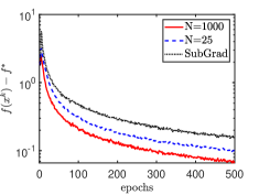
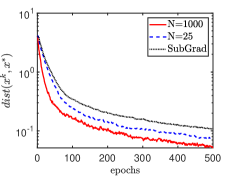
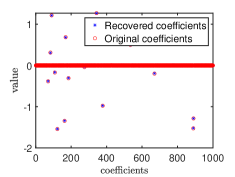
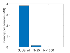
Figure 1: Experiments on the robust M-estimators problem with $\ell_{1}$-loss and $\ell_{1}$-penalty. Top-left: $f(x^{k})-f^{*}$ versus epoch counts for different choices of $N$ (i.e., the number of blocks in RCS); Top-right: $\operatorname{dist}(x^{k},x^{*})$ versus epoch counts for different choices of $N$; Bottom-left: Coefficients recovery by RCS with $N=d$; Bottom-right: Comparison on workspace memory consumption per iteration. Here, $n=500$, $d=1000$, $s=20$, $p_{\mbox{fail}}=0.2$.

Table 1: RCS versus SubGrad on linear SVM.

Data set	RCS		SubGrad
($n/d$)	$f(x^{k})$	memory (MB)	$f(x^{k})$	memory (MB)
colon-cancer ($62/2000$)	0.0379	0.0024	0.0399	1.9698
duke ($44/7129$)	0.0078	0.0017	0.0719	5.0593
leu ($38/7129$)	0.0062	0.0015	0.1325	4.4065
gisette-scale.t ($1000/5000$)	0.1270	0.0382	0.3166	76.5076
a1a ($1605/119$)	0.5762	0.0613	0.5762	2.9557
a2a ($2265/119$)	0.5896	0.0865	0.5896	4.1692
a3a ($3185/122$)	0.5718	0.1216	0.5718	6.0067
a4a ($4781/122$)	0.5821	0.1824	0.5821	9.0143

7.2 Linear SVM problem

We compare RCS (set $N=d$) with SubGrad on the linear SVM problem (3) (i.e., Application 2). We repeat the problem in the following for convenience:

$$\min_{x\in\mathbb{R}^{d}}\ f(x):=\frac{1}{n}\sum_{i=1}^{n}\max\left\{0,1-b_{i}(a_{i}^{\top}x)\right\}+\frac{p}{2}\|x\|^{2}.$$

where $a_{i}\in\mathbb{R}^{d}$ is a vector, $b_{i}\in\mathbb{R}$ is a scalar, $p>0$ is a positive number.

Let $A=\left(a_{1},...,a_{n}\right)^{\top}\in\mathbb{R}^{n\times d}$ be the data matrix and $b=\left(b_{1},...,b_{n}\right)^{\top}\in\mathbb{R}^{n}$ be a vector. We define $\mathbb{R}^{n\times d}\ni\tilde{A}=(b\mathbf{1}_{d}^{\top})\circ A$, where $\mathbf{1}_{d}$ is a $d$-dimensional vector of all $1$s and $\circ$ is the Hadamard product. To implement RCS, we introduce the block-wise partition of the columns of the matrix $\tilde{A}=\left(\tilde{A}_{1},\tilde{A}_{2},\cdots,\tilde{A}_{N}\right)$, where $\tilde{A}_{i}\in\mathbb{R}^{n\times d_{i}}$ is the $i$-th block. Then, it is key to compute the coordinate subgradient $r^{k}_{i(k)}$, which can be calculated as:

$$\left\{\begin{aligned} &r_{i(k)}^{k}=-\frac{1}{n}\tilde{A}_{i(k)}^{\top}\max\{0,\operatorname{sign}(s^{k})\}+px_{i(k)}^{k},\\ &s^{k+1}=s^{k}+\tilde{A}_{i(k)}(x_{i(k)}^{k}-x_{i(k)}^{k+1}),\end{aligned}\right.$$

where $s^{0}=\mathbf{1}_{n}-\tilde{A}x^{0}$.

We use the real datasets from LIBSVM [40] to test the algorithms. The termination criterion for all algorithms is $200$ epochs. We display the results in Table 1, from which we can observe that RCS outperforms SubGrad in terms of both the returned objective value and workspace memory consumption (per iteration).

7.3 Robust phase retrieval problem

initial image (initial point)

SubGrad after $10$ epochs

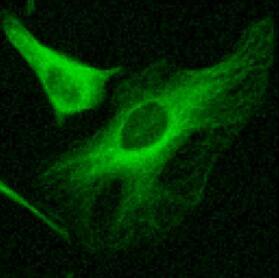
RCS after $10$ epochs

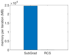
memory per iteration (MB)

Figure 2: Experiments on the robust phase retrieval problem with gold nanoparticles correlative images.

We compare RCS (set $N=d$) with SubGrad on the robust phase retrieval problem (4) (i.e., Application 3). We display the problem below for convenience.

$$\min_{x\in\mathbb{R}^{d}}\ f(x):=\frac{1}{n}\|(Ax)^{\circ 2}-b^{\circ 2}\|_{1},$$

where $A=\left(a_{1},...,a_{n}\right)^{\top}\in\mathbb{R}^{n\times d}$ is the data matrix, $b=\left(b_{1},...,b_{n}\right)^{\top}\in\mathbb{R}^{n}$ is a vector, $\circ$ represents the Hadamard product, and $\circ 2$ is the Hadamard power.

To implement RCS, we introduce the block-wise partition of the columns of the matrix ${A}=\left({A}_{1},{A}_{2},\cdots,{A}_{N}\right)$, where $A_{i}\in\mathbb{R}^{n\times d_{i}}$ is the $i$-th block. Then, the coordinate subgradient $r_{i(k)}^{k}$ used in RCS can be computed as:

$$\left\{\begin{aligned} &r_{i(k)}^{k}=\frac{2}{n}A_{i(k)}^{\top}\left(s^{k}\circ\operatorname{sign}((s^{k})^{\circ 2}-b^{\circ 2})\right),\\ &s^{k+1}=s^{k}+A_{i(k)}(x_{i(k)}^{k+1}-x_{i(k)}^{k}),\end{aligned}\right.$$

where $s^{0}=Ax^{0}$.

To test the algorithms, we use the gold nanoparticles correlative images from [41] as the true solution $x^{*}\in\mathbb{R}^{d}$. Let $H\in\{-1,1\}^{d\times d}/\sqrt{d}$ be a symmetric normalized Hadamard matrix which satisfies the equation $H^{2}=I_{d}$. For some integer $m$, we generate $m$ i.i.d. diagonal sign matrices $S_{1},...,S_{m}\in\mathrm{diag}(\{-1,1\}^{d})$ uniformly at random, and define $n=md$ and $A=\left(a_{1},...,a_{n}\right)^{\top}=\left[HS_{1},HS_{2},...,HS_{m}\right]^{\top}\in\mathbb{R}^{n\times d}$. Next we generate the outlier vector $\delta=(\delta_{1},...,\delta_{n})^{\top}\in\mathbb{R}^{n}$. We randomly select $p_{\mbox{fail}}\cdot n$ locations. Then, we fill each of the selected locations with an i.i.d. $\mathcal{N}(0,1000)$ Gaussian distribution, while the remaining locations are set to $0$. Here, $p_{\mbox{fail}}$ is the ratio of outliers. The measurement vector $(b_{1}^{2},...,b_{n}^{2})^{\top}\in\mathbb{R}^{n}$ is obtained by $b_{i}^{2}=\left\{\begin{array}[]{lc}(a_{i}^{\top}x^{*})^{2}&\delta_{i}=0\\ \delta_{i}&\delta_{i}\neq 0\end{array}\right.$, for $i=1,...,n$.

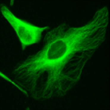
original image

initial image (initial point)

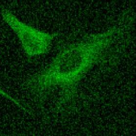
RCS after $5$ epochs

RCS after $10$ epochs

RCS after $15$ epochs

RCS after $20$ epochs

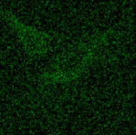
SubGrad after $5$ epochs

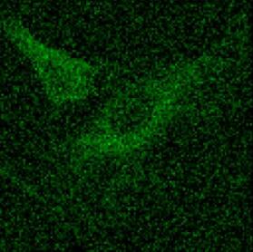
SubGrad after $10$ epochs

SubGrad after $15$ epochs

SubGrad after $20$ epochs

Figure 5: A supplemental to Figure 2 by showing more epochs.

In Figure 2, we can see that RCS with just 10 epochs outputs a much clearer retrieved image than the 10 epochs’ output of SubGrad. In addition, RCS requires much less workspace memory than SubGrad per iteration. These properties of RCS are crucial for solving such a huge-scale problem since performing one iteration of SubGrad can be intractable in the scenario where the computational sources are limited. Actually, this is exactly the reason why we do not perform this simulation on the device used for the previous two examples as performing one iteration of SubGrad causes out of memory issue if we use the personal computer. More epochs are displayed in Figure 5.

8 Conclusion

In this paper, we introduced RCS for solving nonsmooth convex and weakly convex composite optimization problems. We considered a general linearly bounded subgradients assumption and conducted a thorough convergence analysis. We also derived a convergence lemma, the relationship between the global metric subregularity properties of a weakly convex function and its Moreau envelope, and the global metric subregularity of the (real-valued) robust phase retrieval problem, which are of independent interests. Moreover, we conducted several experiments to show the superiority of RCS over the subgradient method. Our work reveals a provable and efficient subgradient-type method for a general class of large-scale nonsmooth composite optimization problems.

Appendix A Appendix

A.1 Proof of Lemma 5.1

Taking $x=x^{*}$ in part (b) of Lemma 3.1 and by the convexity of $f$, we can compute

$$\mathbb{E}_{i(k)}\left[\|x^{k+1}-x^{*}\|^{2}\right]\leq \|x^{k}-x^{*}\|^{2}+\frac{\alpha_{k}^{2}}{N}(L_{1}\|x^{k}\|+L_{2})^{2}-\frac{2\alpha_{k}}{N}(f(x^{k})-f^{*})$$

$$\leq \|x^{k}-x^{*}\|^{2}+\frac{\alpha_{k}^{2}}{N}(2L_{1}^{2}\|x^{k}\|^{2}+2L_{2}^{2})-\frac{2\alpha_{k}}{N}(f(x^{k})-f^{*})$$

$$\leq \|x^{k}-x^{*}\|^{2}+\frac{\alpha_{k}^{2}}{N}\left(4L_{1}^{2}\|x^{*}-x^{k}\|^{2}+4L_{1}^{2}\|x^{*}\|^{2}+2L_{2}^{2}\right)-\frac{2\alpha_{k}}{N}(f(x^{k})-f^{*}),$$

which yields the desired result.

A.2 Proof of Theorem 5.2

By Lemma 5.3, we have

$$\mathbb{E}_{\mathcal{F}_{k}}[\operatorname{dist}^{2}(x^{k+1},\mathbb{X}^{*})]-\mathbb{E}_{\mathcal{F}_{k-1}}[\operatorname{dist}^{2}(x^{k},\mathbb{X}^{*})]\leq\frac{C_{1}}{N}\alpha_{k}^{2}-\frac{2\alpha_{k}}{N}\mathbb{E}_{\mathcal{F}_{k-1}}(f(x^{k})-f^{*}).$$

Since $f$ satisfy the global quadratic growth condition with $\kappa_{3}$, we obtain

$$\mathbb{E}_{\mathcal{F}_{k}}[\operatorname{dist}^{2}(x^{k+1},\mathbb{X}^{*})]-\mathbb{E}_{\mathcal{F}_{k-1}}[\operatorname{dist}^{2}(x^{k},\mathbb{X}^{*})]\leq\frac{C_{1}}{N}\alpha_{k}^{2}-\frac{2\alpha_{k}}{N\kappa_{3}}\mathbb{E}_{\mathcal{F}_{k-1}}[\operatorname{dist}^{2}(x^{k},\mathbb{X}^{*})].$$ (42)

Let $\alpha_{k}=\frac{N\kappa_{3}}{k+1}$. (42) reduces to

$$\mathbb{E}_{\mathcal{F}_{k}}[\operatorname{dist}^{2}(x^{k+1},\mathbb{X}^{*})]-\mathbb{E}_{\mathcal{F}_{k-1}}[\operatorname{dist}^{2}(x^{k},\mathbb{X}^{*})]\\ \leq\frac{NC_{1}\kappa_{3}^{2}}{(k+1)^{2}}-\frac{2}{k+1}\mathbb{E}_{\mathcal{F}_{k-1}}[\operatorname{dist}^{2}(x^{k},\mathbb{X}^{*})].$$

Multiplying both sides of the above inequality by $(k+1)^{2}$ gives

$$(k+1)^{2}\mathbb{E}_{\mathcal{F}_{k}}[\operatorname{dist}^{2}(x^{k+1},\mathbb{X}^{*})]-\left[(k+1)^{2}-2k-2\right]\mathbb{E}_{\mathcal{F}_{k-1}}[\operatorname{dist}^{2}(x^{k},\mathbb{X}^{*})]\leq NC_{1}\kappa_{3}^{2}.$$

Note the fact that $(k+1)^{2}-2k-2=k^{2}-1\leq k^{2}$. Then, we further have

$$(k+1)^{2}\mathbb{E}_{\mathcal{F}_{k}}[\operatorname{dist}^{2}(x^{k+1},\mathbb{X}^{*})]-k^{2}\mathbb{E}_{\mathcal{F}_{k-1}}[\operatorname{dist}^{2}(x^{k},\mathbb{X}^{*})]\leq NC_{1}\kappa_{3}^{2}.$$

Therefore,

$$(k+1)^{2}\mathbb{E}_{\mathcal{F}_{k}}[\operatorname{dist}^{2}(x^{k+1},\mathbb{X}^{*})]= \sum_{j=0}^{k}\bigg{[}(j+1)^{2}\mathbb{E}_{\mathcal{F}_{j}}[\operatorname{dist}^{2}(x^{j+1},\mathbb{X}^{*})]-j^{2}\mathbb{E}_{\mathcal{F}_{j-1}}[\operatorname{dist}^{2}(x^{j},\mathbb{X}^{*})]\bigg{]}$$

$$\leq NC_{1}\kappa_{3}^{2}(k+1),$$

which yields

$$\mathbb{E}_{\mathcal{F}_{k}}[\operatorname{dist}^{2}(x^{k+1},\mathbb{X}^{*})]\leq\frac{NC_{1}\kappa_{3}^{2}}{k+1}.$$

A.3 Proof of 6.1

The robust phase retrieval problem (4) can be rewritten as

$$\min_{x\in\mathbb{R}^{d}}\quad f(x)=\frac{1}{n}\|(Ax)^{\circ 2}-b^{\circ 2}\|_{1}=\frac{1}{n}\sum_{i=1}^{n}|\left(a_{i}^{\top}x\right)^{2}-b_{i}^{2}|,$$ (43)

where $A=\left(a_{1},...,a_{n}\right)^{\top}\in\mathbb{R}^{n\times d}$, $b=(b_{1},...,b_{n})^{\top}\in\mathbb{R}^{n}$ and $\circ 2$ is the Hadamard power. And the subgradient of robust phase retrieval problem is

$$\partial f(x)=\frac{2}{n}A^{\top}\left(Ax\circ\xi\right)=\frac{2}{n}\sum_{i=1}^{n}a_{i}\left(a_{i}^{\top}x\cdot\xi_{i}\right)\quad\mbox{with}\quad\xi=\left(\xi_{1},...,\xi_{n}\right)^{\top},$$

$\xi_{i}\in\left\{\begin{aligned} \{-1\}&\qquad(a_{i}^{\top}x)^{2}-b_{i}^{2}<0\\ [-1,1]&\qquad(a_{i}^{\top}x)^{2}-b_{i}^{2}=0\\ \{1\}&\qquad(a_{i}^{\top}x)^{2}-b_{i}^{2}>0\end{aligned}\right.$, and $\circ$ is the Hadamard product.

Intuitively, for any given $x\in\mathbb{R}^{d}$, we can divided the index of datasets $\{(a_{1},b_{1}),...,(a_{n},b_{n})\}$ into three subsets:

$$\mathbb{I}_{1} =\{i\in\{1,...,n\}|(a_{i}^{\top}x)^{2}=b_{i}^{2}\},$$ (44)

$$\mathbb{I}_{2} =\{i\in\{1,...,n\}|(a_{i}^{\top}x)^{2}>b_{i}^{2}\},$$

$$\mathbb{I}_{3} =\{i\in\{1,...,n\}|(a_{i}^{\top}x)^{2}<b_{i}^{2}\}.$$

We can easily find the fact that $\mathbb{I}_{1}\cap\mathbb{I}_{2}=\emptyset$, $\mathbb{I}_{2}\cap\mathbb{I}_{3}=\emptyset$, $\mathbb{I}_{1}\cap\mathbb{I}_{3}=\emptyset$, and $\mathbb{I}_{1}\cup\mathbb{I}_{2}\cup\mathbb{I}_{3}=\{1,...,n\}$. For given $x\in\mathbb{R}^{d}$, the subdifferential of robust phase retrieval problem can be rewritten as

$$\partial f(x)=\frac{2}{n}\left[\sum_{i\in\mathbb{I}_{1}}a_{i}\left(a_{i}^{\top}x\cdot[-1,1]\right)+\sum_{i\in\mathbb{I}_{2}}a_{i}a_{i}^{\top}x-\sum_{i\in\mathbb{I}_{3}}a_{i}a_{i}^{\top}x\right].$$ (45)

If $x=\bar{x}\in\overline{\mathbb{X}}$, (45) yields that

$$\sum_{i\in\mathbb{I}_{2}}a_{i}a_{i}^{\top}\bar{x}=\sum_{i\in\mathbb{I}_{3}}a_{i}a_{i}^{\top}\bar{x}-\sum_{i\in\mathbb{I}_{1}}a_{i}\left(a_{i}^{\top}\bar{x}\cdot\delta_{i}\right),$$ (46)

with $\delta_{i}\in[-1,1]$, $i=1,...,n$. By the full column rank of $A$, we denote the positive definite matrix $Q=A^{\top}A$, and $\sigma_{min}(Q^{\top}Q)$ be the minimum eigenvalue of matrix $Q^{\top}Q$. Then we can derive that

$$\sqrt{\sigma_{\min}(Q^{\top}Q)}\|\bar{x}\|\leq \|A^{\top}A\bar{x}\|$$ (47)

$$= \|\sum_{i=1}^{n}a_{i}a_{i}^{\top}\bar{x}\|$$

$$= \|\sum_{i\in\mathbb{I}_{1}}a_{i}a_{i}^{\top}\bar{x}+\sum_{i\in\mathbb{I}_{2}}a_{i}a_{i}^{\top}\bar{x}+\sum_{i\in\mathbb{I}_{3}}a_{i}a_{i}^{\top}\bar{x}\|$$

$$= \|2\sum_{i\in\mathbb{I}_{3}}a_{i}a_{i}^{\top}\bar{x}+\sum_{i\in\mathbb{I}_{1}}a_{i}a_{i}^{\top}\bar{x}-\sum_{i\in\mathbb{I}_{1}}a_{i}\left(a_{i}^{\top}\bar{x}\cdot\delta_{i}\right)\|\quad\mbox{(by~{}\eqref{eq:pr_bd_2})}$$

$$\leq 2\sum_{i\in\mathbb{I}_{3}}\|a_{i}\|\cdot|a_{i}^{\top}\bar{x}|+2\sum_{i\in\mathbb{I}_{1}}\|a_{i}\|\cdot|a_{i}^{\top}\bar{x}|.$$

By (44), we have $|a_{i}^{\top}\bar{x}|=|b_{i}|$, $\forall i\in\mathbb{I}_{1}$ and $|a_{i}^{\top}\bar{x}|<|b_{i}|$, $\forall i\in\mathbb{I}_{3}$. Then (47) yields that

$$\|\bar{x}\|\leq\frac{2\sum_{i\in\mathbb{I}_{3}}\|a_{i}\|\cdot|b_{i}|+2\sum_{i\in\mathbb{I}_{1}}\|a_{i}\|\cdot|b_{i}|}{\sqrt{\sigma_{\min}(Q^{\top}Q)}}.$$

Therefore, under the assumption that $A$ is full column rank, the critical points set of the robust phase retrieval problem (4) is bounded, i.e., $\max_{\bar{x}\in\overline{\mathbb{X}}}\|\bar{x}\|\leq{\sf B}_{2}=\frac{2\sum_{i\in\mathbb{I}_{3}}\|a_{i}\|\cdot|b_{i}|+2\sum_{i\in\mathbb{I}_{1}}\|a_{i}\|\cdot|b_{i}|}{\sqrt{\sigma_{\min}(Q^{\top}Q)}}$.

A.4 Proof of Corollary 6.1

Note that the step sizes $\alpha_{k}=\frac{\Delta}{\sqrt{k+1}\log(k+2)}$. The two conditions in (24) are automatically satisfied since

$$\sum_{j=0}^{k}\alpha_{j}^{2}\leq\alpha_{0}^{2}+\int_{0}^{k}\frac{\Delta^{2}}{(t+1)\log^{2}(t+2)}dt\leq\frac{2\Delta^{2}}{(\log 2)^{2}},$$

and

$$\sum_{j=0}^{k}\alpha_{j}\geq\sum_{j=0}^{k}\frac{\Delta}{\sqrt{k+1}\log(k+2)}=\frac{\Delta\sqrt{k+1}}{\log(k+2)}.$$

We now prove this corollary by contradiction. Let us assume that the statement does not hold. Then, we have

$$\mathbb{P}\left(\left\{w\in\Omega:\liminf_{k\rightarrow\infty}\ \sqrt{k+1}\|\nabla f_{\lambda}(x^{k}(w))\|^{2}\geq\delta\right\}\right)>0,$$

for some $\delta>0$. Then, there exists a sufficiently large $\overline{k}$ such that

$$\mathbb{P}\left(\left\{w\in\Omega:\sqrt{k+1}\ \|\nabla f_{\lambda}(x^{k}(w))\|^{2}\geq\delta\right\}\right)>0$$

for all $k\geq\overline{k}$. Hence, we have

$$\mathbb{P}\left(\left\{w\in\Omega:\sum_{k=\overline{k}}^{\infty}\frac{1}{\sqrt{k+1}\log(k+2)}\|\nabla f_{\lambda}(x^{k}(w))\|^{2}\geq\sum_{k=\overline{k}}^{\infty}\frac{\delta}{(k+1)\log(k+2)}\right\}\right)>0.$$ (48)

By the integral comparison test, we have $\sum_{k=\overline{k}}^{\infty}\frac{1}{(k+1)\log(k+2)}\geq\int_{\overline{k}+2}^{\infty}\frac{1}{t\log(t)}dt=\infty$. Note that $\alpha_{k}=\frac{\Delta}{\sqrt{k+1}\log(k+2)}$. Therefore, (48) is a contradiction to (41).

A.5 RCS for M-estimators problem with MCP-loss and $\ell_{1}$-penalty, and more experiments

In this subsection, we consider the M-estimators problem (2) with MCP-loss and $\ell_{1}$-penalty, i.e.,

$$\min\limits_{x\in\mathbb{R}^{d}}\ f(x):=\frac{1}{n}\sum_{i=1}^{n}\phi_{p_{1}}(a_{i}^{\top}x-b_{i})+p_{2}\|x\|_{1},$$

where $a_{i}\in\mathbb{R}^{d}$ is a vector, $b_{i}\in\mathbb{R}$ is a scalar, $p_{2}>0$ is the regularization parameter, and $\phi_{p_{1}}(z)=\left\{\begin{array}[]{ll}|z|-\frac{z^{2}}{2p_{1}}&|z|\leq p_{1}\\ \frac{1}{2}p_{1}&|z|>p_{1}\end{array}\right.$ is the MCP-loss.

Let $A=(a_{1},...,a_{n})^{\top}\in\mathbb{R}^{n\times d}$ be a matrix and $b=(b_{1},...,b_{n})^{\top}\in\mathbb{R}^{n}$ be a vector. In order to implement RCS, we introduce the block-wise partition of the columns of the data matrix $A=(A_{1},A_{2},\cdots,A_{N})$, where $A_{i}\in\mathbb{R}^{n\times d_{i}}$ is the $i$-th block. For this problem, the coordinate subgradient used in RCS can be calculated as:

$$\left\{\begin{aligned} &r_{i(k)}^{k}=\frac{1}{n}A_{i(k)}^{\top}u^{k}+p_{2}\operatorname{sign}(x_{i(k)}^{k}),\\ &s^{k+1}=s^{k}+A_{i(k)}(x_{i(k)}^{k+1}-x_{i(k)}^{k}),\end{aligned}\right.$$

where $u^{k}\in\partial\Phi(s^{k})=\left(\partial\phi_{p_{1}}(s_{1}^{k}),...,\partial\phi_{p_{1}}(s_{n}^{k})\right)^{\top}$ with $\partial\phi_{p_{1}}(z)=\left\{\begin{array}[]{ll}\operatorname{sign}(z)-\frac{z}{p_{1}}&|z|\leq p_{1}\\ 0&|z|>p_{1}\end{array}\right.$ and $s^{0}=Ax^{0}-b$.

We conduct our simulation based on the synthetic data generated in Subsection 7.1. In Figure 3 and Figure 4, we show the evolution of $f(x^{k})-f^{*}$ and $\operatorname{dist}(x^{k}-x^{*})$ versus epoch counts with different number of blocks $N$. Similar to the conclusions draw from Figure 1, we can observe that RCS with larger $N$ converges faster than RCS with smaller $N$ and SubGrad. In addition, larger $N$ requires less workspace memory than small $N$ and SubGrad per iteration. Finally, RCS can effectively recover the sparse coefficients.

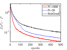
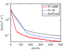
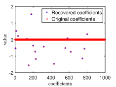
Figure 3: Experiments on Robust M-estimators problem with MCP-loss and $\ell_{1}$-penalty. Top Left: $f(x^{k})-f^{*}$ versus epoch counts for different choices of $N$ (i.e., the number of blocks in RCS); Top Right: $\operatorname{dist}(x^{k},x^{*})$ versus epoch counts for different choices of $N$; Bottom Left: Coefficients recovery by RCS with $N=d$; Bottom Right: Comparison on workspace memory consumption per iteration. Here, $n=500$, $d=1000$, $s=20$, and $p_{\mbox{fail}}=0.25$.

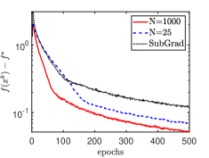
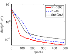
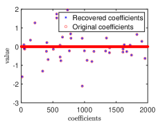
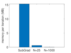
Figure 4: Experiments on Robust M-estimators problem with MCP-loss and $\ell_{1}$-penalty. Top Left: $f(x^{k})-f^{*}$ versus epoch counts for different choices of $N$ (i.e., the number of blocks in RCS); Top Right: $\operatorname{dist}(x^{k},x^{*})$ versus epoch counts for different choices of $N$; Bottom Left: Coefficients recovery by RCS with $N=d$; Bottom Right: Comparison on workspace memory consumption per iteration. Here, $n=1000$, $d=2000$, $s=40$, and $p_{\mbox{fail}}=0.25$.

References

- [1] S. J. Wright, “Coordinate descent algorithms,” Mathematical Programming, vol. 151, no. 1, pp. 3–34, 2015.
- [2] M. A. Kerahroodi, A. Aubry, A. De Maio, M. M. Naghsh, and M. Modarres-Hashemi, “A coordinate-descent framework to design low PSL/ISL sequences,” IEEE Transactions on Signal Processing, vol. 65, no. 22, pp. 5942–5956, 2017.
- [3] A. Vandaele, N. Gillis, Q. Lei, K. Zhong, and I. Dhillon, “Efficient and non-convex coordinate descent for symmetric nonnegative matrix factorization,” IEEE Transactions on Signal Processing, vol. 64, no. 21, pp. 5571–5584, 2016.
- [4] P. Tseng, “Convergence of a block coordinate descent method for nondifferentiable minimization,” Journal of optimization theory and applications, vol. 109, no. 3, pp. 475–494, 2001.
- [5] Y. Nesterov, “Efficiency of coordinate descent methods on huge-scale optimization problems,” SIAM Journal on Optimization, vol. 22, no. 2, pp. 341–362, 2012.
- [6] P. Richtárik and M. Takáč, “Iteration complexity of randomized block-coordinate descent methods for minimizing a composite function,” Mathematical Programming, vol. 144, no. 1-2, pp. 1–38, 2014.
- [7] A. Beck and L. Tetruashvili, “On the convergence of block coordinate descent type methods,” SIAM journal on Optimization, vol. 23, no. 4, pp. 2037–2060, 2013.
- [8] Z. Lu and L. Xiao, “On the complexity analysis of randomized block-coordinate descent methods,” Mathematical Programming, vol. 152, no. 1-2, pp. 615–642, 2015.
- [9] D. Zhu and L. Zhao, “Linear convergence of randomized primal-dual coordinate method for large-scale linear constrained convex programming,” in International Conference on Machine Learning. PMLR, 2020, pp. 11 619–11 628.
- [10] J. Liu and S. J. Wright, “Asynchronous stochastic coordinate descent: Parallelism and convergence properties,” SIAM Journal on Optimization, vol. 25, no. 1, pp. 351–376, 2015.
- [11] A. S. Lewis and S. J. Wright, “A proximal method for composite minimization,” Mathematical Programming, vol. 158, pp. 501–546, 2016.
- [12] J. C. Duchi and F. Ruan, “Stochastic methods for composite and weakly convex optimization problems,” SIAM Journal on Optimization, vol. 28, no. 4, pp. 3229–3259, 2018.
- [13] D. Davis and D. Drusvyatskiy, “Stochastic model-based minimization of weakly convex functions,” SIAM Journal on Optimization, vol. 29, no. 1, pp. 207–239, 2019.
- [14] D. Drusvyatskiy and C. Paquette, “Efficiency of minimizing compositions of convex functions and smooth maps,” Mathematical Programming, vol. 178, no. 1-2, pp. 503–558, 2019.
- [15] P.-L. Loh and M. J. Wainwright, “Regularized m-estimators with nonconvexity: Statistical and algorithmic theory for local optima,” The Journal of Machine Learning Research, vol. 16, no. 1, pp. 559–616, 2015.
- [16] C.-H. Zhang et al., “Nearly unbiased variable selection under minimax concave penalty,” The Annals of statistics, vol. 38, no. 2, pp. 894–942, 2010.
- [17] J. Fan and R. Li, “Variable selection via nonconcave penalized likelihood and its oracle properties,” Journal of the American statistical Association, vol. 96, no. 456, pp. 1348–1360, 2001.
- [18] C. Cortes and V. Vapnik, “Support-vector networks,” Machine learning, vol. 20, no. 3, pp. 273–297, 1995.
- [19] Y. Zhang and X. Lin, “Stochastic primal-dual coordinate method for regularized empirical risk minimization,” in International Conference on Machine Learning. PMLR, 2015, pp. 353–361.
- [20] J. R. Fienup, “Phase retrieval algorithms: a comparison,” Applied optics, vol. 21, no. 15, pp. 2758–2769, 1982.
- [21] J. C. Duchi and F. Ruan, “Solving (most) of a set of quadratic equalities: Composite optimization for robust phase retrieval,” Information and Inference: A Journal of the IMA, vol. 8, no. 3, pp. 471–529, 2019.
- [22] Y. Nesterov, “Subgradient methods for huge-scale optimization problems,” Mathematical Programming, vol. 146, no. 1-2, pp. 275–297, 2014.
- [23] C. D. Dang and G. Lan, “Stochastic block mirror descent methods for nonsmooth and stochastic optimization,” SIAM Journal on Optimization, vol. 25, no. 2, pp. 856–881, 2015.
- [24] G. Cohen and D. Zhu, “Decomposition and coordination methods in large scale optimization problems: The nondifferentiable case and the use of augmented lagrangians,” Adv. in Large Scale Systems, vol. 1, pp. 203–266, 1984.
- [25] J.-C. Culioli and G. Cohen, “Decomposition/coordination algorithms in stochastic optimization,” SIAM Journal on Control and Optimization, vol. 28, no. 6, pp. 1372–1403, 1990.
- [26] H. Lu, “"Relative continuity" for non-lipschitz nonsmooth convex optimization using stochastic (or deterministic) mirror descent,” INFORMS Journal on Optimization, vol. 1, no. 4, pp. 288–303, 2019.
- [27] Y. Zhou, V. Sanches Portella, M. Schmidt, and N. Harvey, “Regret bounds without lipschitz continuity: online learning with relative-lipschitz losses,” Advances in Neural Information Processing Systems, vol. 33, pp. 15 823–15 833, 2020.
- [28] J. Renegar, “"Efficient" subgradient methods for general convex optimization,” SIAM Journal on Optimization, vol. 26, no. 4, pp. 2649–2676, 2016.
- [29] B. Grimmer, “Radial subgradient method,” SIAM Journal on Optimization, vol. 28, no. 1, pp. 459–469, 2018.
- [30] B. Grimmer, “Convergence rates for deterministic and stochastic subgradient methods without lipschitz continuity,” SIAM Journal on Optimization, vol. 29, no. 2, pp. 1350–1365, 2019.
- [31] N. Z. Shor, Minimization methods for non-differentiable functions. Springer Science & Business Media, 2012, vol. 3.
- [32] J.-P. Vial, “Strong and weak convexity of sets and functions,” Mathematics of Operations Research, vol. 8, no. 2, pp. 231–259, 1983.
- [33] R. T. Rockafellar and R. J.-B. Wets, Variational analysis. Springer Science & Business Media, 2009, vol. 317.
- [34] D. Zhu, S. Deng, M. Li, and L. Zhao, “Level-set subdifferential error bounds and linear convergence of bregman proximal gradient method,” in Journal of Optimization Theory and Applications. Springer, 2021, pp. 1–30.
- [35] H. Robbins and D. Siegmund, “A convergence theorem for non negative almost supermartingales and some applications,” in Optimizing methods in statistics. Elsevier, 1971, pp. 233–257.
- [36] X. Li, Z. Zhu, A. Man-Cho So, and R. Vidal, “Nonconvex robust low-rank matrix recovery,” SIAM Journal on Optimization, vol. 30, no. 1, pp. 660–686, 2020.
- [37] A. L. Dontchev and R. T. Rockafellar, Implicit functions and solution mappings. Springer, 2009, vol. 543.
- [38] X. Y. Zheng and K. F. Ng, “Metric subregularity of piecewise linear multifunctions and applications to piecewise linear multiobjective optimization,” SIAM Journal on Optimization, vol. 24, no. 1, pp. 154–174, 2014.
- [39] I. Necoara, Y. Nesterov, and F. Glineur, “Linear convergence of first order methods for non-strongly convex optimization,” Mathematical Programming, vol. 175, no. 1, pp. 69–107, 2019.
- [40] C.-C. Chang and C.-J. Lin, “Libsvm: A library for support vector machines,” ACM transactions on intelligent systems and technology (TIST), vol. 2, no. 3, p. 27, 2011.
- [41] M. Liu, Q. Li, L. Liang, J. Li, K. Wang, J. Li, M. Lv, N. Chen, H. Song, J. Lee, J. Shi, L. Wang, R. Lal, and C. Fan, “Real-time visualization of clustering and intracellular transport of gold nanoparticles by correlative imaging,” Nature Communications, vol. 8, no. 1, pp. 1–10, 2017.