GLD-Net: Improving Monaural Speech Enhancement by Learning Global and Local Dependency Features with GLD Block

Abstract

For monaural speech enhancement, contextual information is important for accurate speech estimation. However, commonly used convolution neural networks (CNNs) are weak in capturing temporal contexts since they only build blocks that process one local neighborhood at a time. To address this problem, we learn from human auditory perception to introduce a two-stage trainable reasoning mechanism, referred as global-local dependency (GLD) block. GLD blocks capture long-term dependency of time-frequency bins both in global level and local level from the noisy spectrogram to help detecting correlations among speech part, noise part, and whole noisy input. What is more, we conduct a monaural speech enhancement network called GLD-Net, which adopts encoder-decoder architecture and consists of speech object branch, interference branch, and global noisy branch. The extracted speech feature at global-level and local-level are efficiently reasoned and aggregated in each of the branches. We compare the proposed GLD-Net with existing state-of-art methods on WSJ0 and DEMAND dataset. The results show that GLD-Net outperforms the state-of-the-art methods in terms of PESQ and STOI.

Index Terms: monaural speech enhancement, global and local dependency, encoder-decoder architecture, two-stage trainable reasoning mechanism

1 Introduction

It has been a long-standing topic in speech processing applications to reduce background noise and improve quality and intelligibility of degraded speech. Speech enhancement is frequently used as the preprocessor of the other acoustic tasks, such as speech recognition [1], cochlear implants [2], and hearing aids [3]. Monaural speech enhancement provides a versatile and cost-effective approach to the problem by utilizing recordings from a single microphone.

Traditional monaural speech enhancement approaches can include Spectral Subtraction [4], minimum mean-square error (MMSE) estimation [5], Wiener filter (linear MMSE) [6], Kalman filter [7], subspace method [8], etc. However, these kinds of speech enhancement methods generally do not perform well in adverse noise environments. In recent years, deep neural networks (DNNs) have shown their promising performance on monaural speech enhancement even in highly non-stationary noise environments because of their superior capability in modeling complex non-linearity.

Most of current deep learning architectures for speech enhancement are implemented in time-frequency (T-F) domain by using short-time Fourier transform (STFT), those methods usually treat the spectral magnitude as training target. The phase of noisy speech is utilized along with the enhanced speech magnitude to reconstruct the time-domain signal with inverse short-time Fourier transform (iSTFT) [9, 10, 11]. Many researchers have investigated the convolution neural network (CNN) or recurrent neural network (RNN). For modeling long-range sequence like speech, CNN requires more convolutional layers to enlarge receptive field. Additionally, although RNN such as long short-term memory (LSTM) or gated recurrent units (GRU) are commonly used in modeling long-term sequence with order information, they cannot perform parallel processing and lead to high computation complexity. Recently, some improvement is achieved by adding temporal convolutional network (TCN) [12] blocks or LSTM layers between encoder and decoder for further extracting high-level features and enlarging receptive fields [13]. However, the contextual information of observed noisy speech is often ignored, which restricts the denoising performance.

To tackle the limitations above, we propose a trainable mechanism to infer speech enhancement which contains a two-stage reasoning process according to the human auditory perception. It is noted that human auditory system is able to identify non-speech sounds and human speech through category-selective responses by capturing long-term context-dependency from the scene and related speech regions [14], which was particularly selective for acoustic-phonetic content of speech [15]. Considering the concert (i.e. instrument sounds and human talk) as an example, the global-level sound information from the scene (e.g. instrument sounds and mixed speech) can be first captured as prior knowledge and the speech from the target person is then learned and selected for further processes. Following this perception, we propose a two-stage mechanism to infer speech enhancement where global and local dependency of time-frequency (T-F) bins of speech spectrogram are captured. Aggregating this innovation synthetically, we propose GLD-Net. The contributions of this work are summarized as follows:

• A two-stage reasoning mechanism is proposed to learn long-term dependency of T-F bins both in global level and local level from the noisy spectrogram to help detecting interactions between speech part and whole noisy scene.

• An efficient framework for monaural speech enhancement is introduced to efficiently assemble GLD block, namely GLD-Net. The GLD-Net consists of a speech object branch, interference noise branch, and a global noisy branch. In particular, the GLD-Net takes encoder-decoder architecture and the GLD block is inserted in encoder part. In addition, a local-attention is utilized in speech object branch, and interference branch of GLD-Net to detect speech region and filter the noise relevant features, respectively.

• To evaluate the proposed GLD-Net, we perform comprehensive ablation studies on public available speech data. Results show that GLD-Net outperforms all 3 evaluated models.

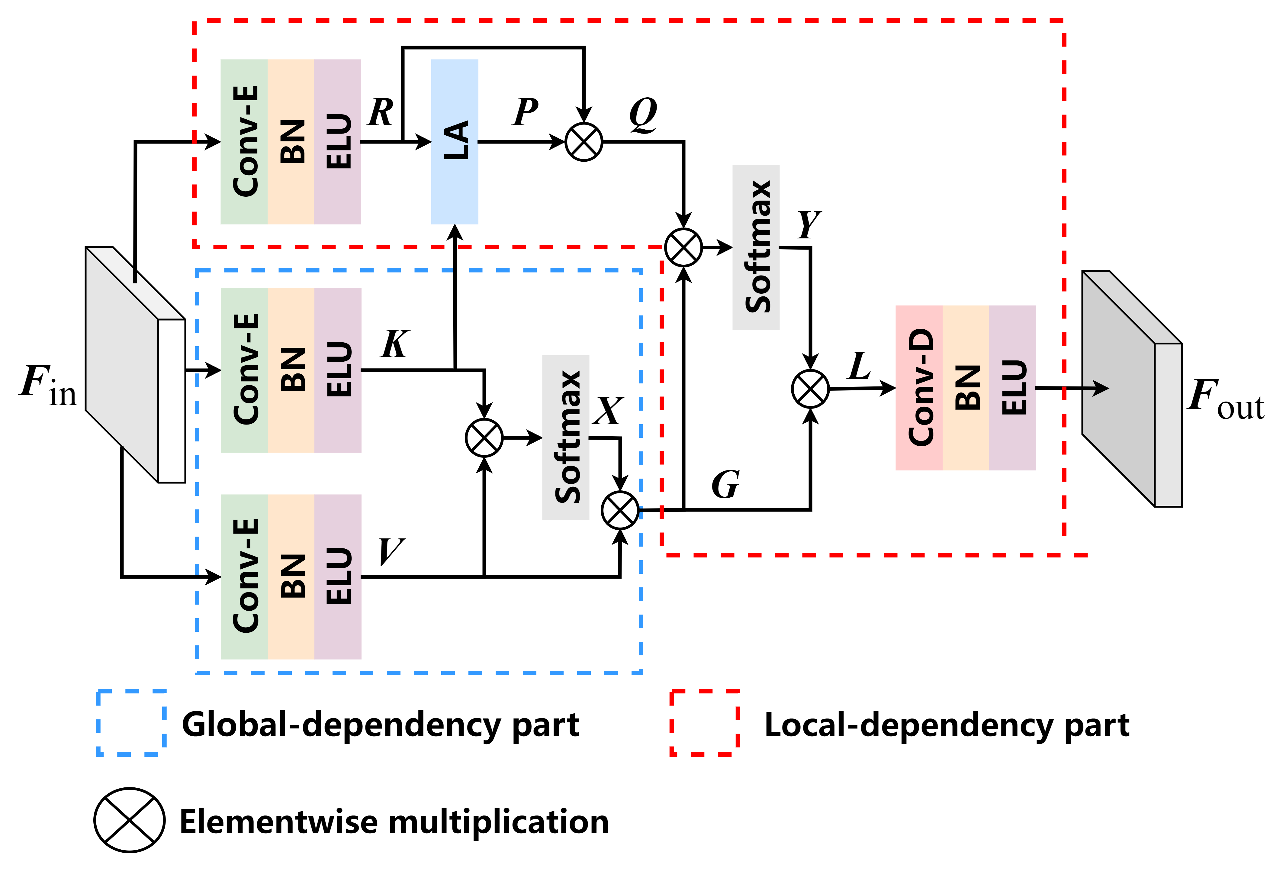
Figure 1: The proposed GLD block in speech branch (one of the three branches from our proposed GLD-Net), where Conv-E, Conv-D, BN, and LA denote convolution encoder, convolution decoder, batch normalization, and local attention, respectively.

2 Model Architecture

2.1 GLD Block

While listening to a target speech, a person is able to capture its long-range context information from the scene and target speech, rather than just orderly focus on target region of the speech signal like convolution operations do. Thus, we learn from human auditory perception to build a two-stage reasoning mechanism which captures long-range dependency in global-level and local-level to predict target speech. To make the above assumption computationally feasible, we design the GLD block containing two parts to exploit both global and local dependency. Taking speech branch (one of three branches from our proposed GLD-Net) as an example, Figure 1 shows the detailed procedure of GLD block.

We divide the process of GLD block into two parts, which are global-dependency part and the local-dependency part. While a speech happens throughout the whole noisy observation, we firstly capture global dependency from the whole noisy speech through the global-dependency part. Afterwards, we capture local dependency from speech region through the local-dependency part.

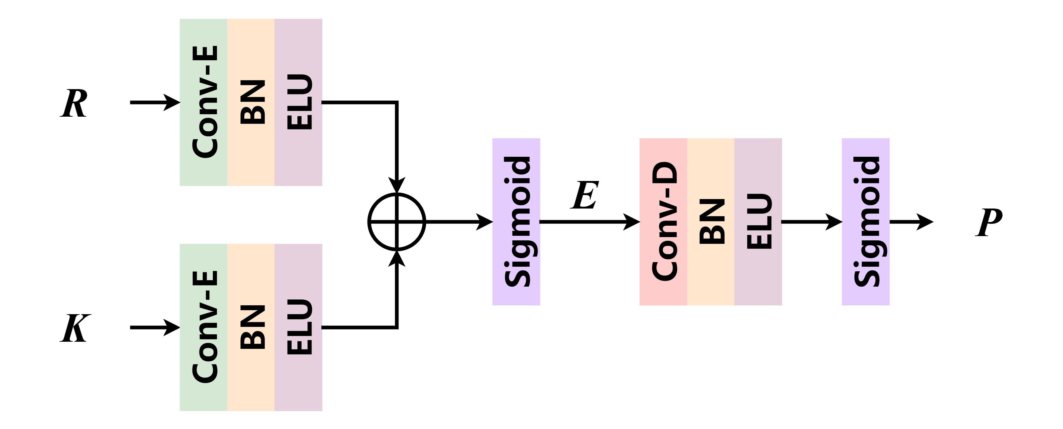
Figure 2: The schematic diagram of local attention.

2.1.1 Global-dependency part

In global-dependency part, given an input feature map $F_{\text{in}}$, two 2D convolution layers, each of which is followed by batch normalization [16] and exponential linear unit (ELU) [17], are adopt to generate new feature map K and V respectively, where $\{\textbf{K},\textbf{V}\}\in\mathbb{R}^{T\times F\times C}$, and $T$, $F$, and $C$ denote the number of time steps, frequency bands, and convolution channels. Concretely, a matrix multiplication between K, $\textbf{V}^{\top}$ is operated, and to obtain the attention map X, a softmax layer is connected as:

$$x_{ji}=\frac{exp(K_{i}\times V_{j})}{\sum^{C}_{i=1}exp(K_{i}\times V_{j})},$$ (1)

in which $x_{ji}$ means the $i^{th}$ channel’s influence on the $j^{th}$ channel. The closer feature representation of the two bins signifies a stronger correlation between them.

Finally, the results of matrix multiplication between $\textbf{X}^{\top}$ and V are weighted by a parameter of scale $\alpha$ to acquire the output of global-dependency part G:

$$G_{j}=\alpha\sum^{C}_{i=1}(x_{ji}V_{j}),$$ (2)

where $\alpha$ is initialized as zero and can be learned gradually.

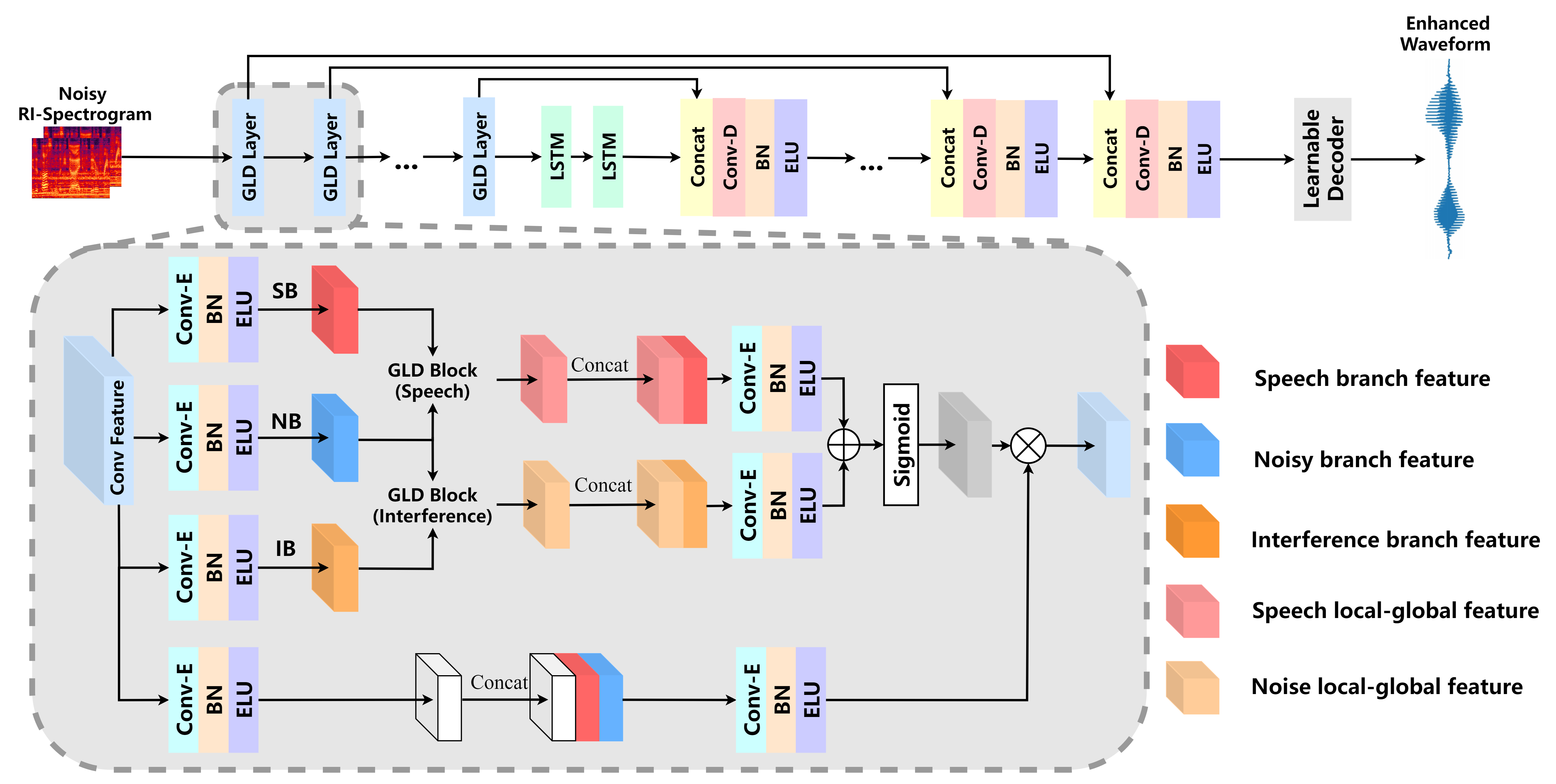
Figure 3: The proposed GLD-Net, where “SB”, “NB”, and “IB” denote speech branch, noisy branch, and interference branch, respectively.

2.1.2 Local-dependency part

In local-dependency part, the intermediate feature map G is computed from the output of global-dependency part, G, and feature map Q which is computed from initial input $F_{\text{in}}$ processing by a 2D convolution block and a local attention (LA).

The LA [18] is described in Figure 2. E is the $F_{\text{in}}$ processing by the 2D convolution block, and K is the feature map in the global-dependency part. Two additional 2D convolution block, referring as $\textbf{W}_{g}^{att}$ and $\textbf{W}_{x}^{att}$, are used to mapping E and K to high-dimensional space feature:

$$\textbf{R}=\sigma(\textbf{W}_{g}^{att}\textbf{E}^{\top}+\textbf{W}_{x}^{att}\textbf{K}^{\top}),$$ (3)

which is fed into a single 2D deconvolution block, $\textbf{W}_{f}^{att}$, to give the local attention mask:

$$\textbf{P}=\sigma(\textbf{W}_{f}^{att}\textbf{R}^{\top}),$$ (4)

where $\sigma$ denotes sigmoid function. Then, the feature map Q is generated by

$$\textbf{Q}=\textbf{R}\times\textbf{P},$$ (5)

The local attention is learning a soft voice activity detection (VAD) and is keeping features focus more on the voice activity region [19].

Next, a multiplication of metrics is executed between Q and G, and a softmax layer is attached subsequently to calculate the attention maps Y:

$$y_{ji}=\frac{exp(Q_{i}\times G_{j})}{\sum^{C}_{i=1}exp(Q_{i}\times G_{j})},$$ (6)

where $y_{ji}$ measures the impact of $i^{th}$ bin to the $j^{th}$ bin. Then, a multiplication of metrics is performed between Y and G, and the result is:

$$L_{j}=\beta\sum^{C}_{i=1}(y_{ji}G_{j}),$$ (7)

where $\beta$ with a zero initial value can be learned to assign larger weight gradually. Finally, the result feature map L is fed into a 2D deconvolution block to form the output of the GLD block, $F_{\text{out}}$.

The goal of the matrix multiplications and softmax operation in GLD block is to dynamically conduct target-specfic reasoning and capture long-range dependency for a speech sequence. In addition, different T-F bins are considered in the spectrogram from global-dependency part and local-dependency part.

2.2 GLD-Net

The proposed GLD-Net uses convolutional encoder-decoder structure based on the standard U-Net [20], shown in Figure 3. The encoder contains several GLD layers, which are introduced in Section 2.2.1. The bottleneck consists of two LSTM layers to improve its generalization capabilities [21]. The decoder contains several 2D dilated decovolution blocks [22]. Skip connections are introduced to compensate for information loss during the encoding process.

In addition, the input of GLD-Net is noisy real-imaginary spectrogram computed by short-time Fourier transform (STFT), denoted by $\textbf{Y}_{r,i}\in\mathbb{R}^{T\times F\times 2}$ [23]. The output of GLD-Net, $\textbf{S}_{out}$, is processed by a learnable decoder layer to transform the feature back to the predicted time-domain signal, $\textbf{s}_{pred}\in\mathbb{R}^{N\times 1}$. The network structure of the learnable decoder is designed to be exactly the same as the convolutional implementation of inverse STFT. Specifically, the learnable decoder is a 1D transposed convolution layer whose kernel size and stride are the window length and hop size in the STFT [24, 25].

2.2.1 GLD layer

Each GLD layer of GLD-Net contains three branches, speech branch (SB), noisy branch (NB), and interference branch (IB), as shown in Figure 3. The local-level feature (SB feature and IB feature), and the global-level feature (NB feature) are extracted from incoming convolution feature map by using three 2D convolution blocks. Then, speech local-global feature and noise local-global feature obtained from GLD block are concatenated to SB and IB features, respectively. It is noted that the GLD blocks for SB and IB are different, in which GLD block for SB is as shown in Figure 1 and GLD block for IB which we change the Eq.(5) of GLD block for SB to $\textbf{Q}=(1-\textbf{P})\times\textbf{E}$. The speech and interference branches takes speech T-F features as inputs to encode long-range dependency.

With the feature vectors, two 2D convolution blocks are employed to fuse the concatenated features, then a matrix addition between the two fused features followed by a sigmoid function are operated to generate local-global dependency gate. Next, several convolution blocks are adopted to extract the feature from original input, obtaining the intermediate feature map. After that SB and NB features are concatenated to intermediate feature, and fed into a 2D convolution block to generate the confidence feature. Our motivation for the concatenation above is that the global context and speech region information are both important for extracting the target speech. Finally, the result of multiplication between confidence feature and local-global dependency gate is the output of a GLD layer, and is passed to the next layer.

Table 1: Evaluation results of proposed model compared with baseline models with unseen speakers. BOLD indicates the best result of each column.

Metric	PESQ					STOI (in %)
Test SNR	-5	0	5	10	Avg.	-5	0	5	10	Avg.
Unprocessed	1.37	1.88	2.12	2.49	1.97	57.06	69.33	80.59	87.63	73.40
CRN [13]	2.14	2.49	2.79	3.09	2.63	78.30	88.61	91.11	94.74	88.19
GRN [26]	2.20	2.58	2.84	3.12	2.69	81.45	88.09	92.43	94.96	89.23
T-GSA [27]	2.33	2.70	2.96	3.24	2.81	83.17	89.54	93.47	95.76	90.49
Proposed GLD-Net	2.41	2.86	3.03	3.28	2.90	84.06	90.12	94.28	96.19	91.16

Table 2: Ablation study of proposed model. BOLD indicates the best result of each column.

Metric	PESQ					STOI (in %)
Test SNR	-5	0	5	10	Avg.	-5	0	5	10	Avg.
Unprocessed	1.37	1.88	2.12	2.49	1.97	57.06	69.33	80.59	87.63	73.40
GLD-Net w/o speech branch	2.23	2.59	2.86	3.11	2.70	81.36	88.41	92.21	94.86	89.21
GLD-Net w/o interference branch	2.38	2.84	2.97	3.20	2.85	83.45	89.79	94.06	95.42	90.68
GLD-Net w/o speech and interference branches	2.17	2.48	2.77	3.04	2.62	80.32	88.24	92.05	94.76	88.84
Proposed GLD-Net	2.41	2.86	3.03	3.28	2.90	84.06	90.12	94.28	96.19	91.16

3 Experimental Setup

In our experiments, we evaluate the models on the WSJ0 SI-84 training set [28] including 7138 utterances from 83 speakers (42 males and 41 females). Among these speakers, 6 speakers (3 males and 3 females) are treated as untrained speakers. Hence, we train the models with 77 remaining speakers. To obtain noise-independent models, we select 10 types of noise signals from Demand dataset [29]. For training, 4.5 hours clean speech randomly mix with noises at a signal-to-noise ratio (SNR) that is randomly chosen from $\{-5,-3,0,3,5,7,10\}$dB. The validation and test set are constructed in the same way, using 1.5 hours of clean speech each, where speakers do not overlap in between the three sets. An additional test sets employing unseen noise types is constructed by using the clean test set speech files and two unseen noise types from the NOISE-92 database [30]. For the evaluation, additional unseen SNR conditions of $\{-5,0,5,10\}$dB are employed.

All data are downsampled to 16 kHz and features are extracted by using frames of length 512 with frame shift of 256, and Hann windowing followed by STFT of size $K=512$ with respective zero-padding. Real and imaginary parts of the complex spectrum are divided into separate feature maps, resulting in $C=2$ input channels. The models are trained with the Adam optimizer [31]. The numbers of output channels for the layers in the encoder are changed to 16, 32, 64, 128 and 256 successively, and those for each layer in the decoder to 128, 64, 32, 16 and 1 successively. We set the learning rate to 0.0002. The mean squared error (MSE) is used as the objective function. We train the model with minibatch size of 16.

4 Results and Analysis

Evaluation metrics are short-time objective intelligibility measure (STOI) [32] and perceptual evaluation of speech quality (PESQ) [33]. All metrics are better if higher.

4.1 Overall Performance

Table 1 presents comprehensive evaluations for three baseline models on untrained noises and untrained speakers. The best results in each case are highlighted by boldface. The three selected baseline models are: (1) CRN [13], a CRN speech enhancement model with complex spectral mapping, (2) GRN [26], a gated convolution speech enhancement model with complex spectral mapping, and (3) T-GSA [27], a Gaussian-weighted self-attention based speech enhancement model in frequency domain.

We first compare CRN and GRN, GRN yields significant better STOI and PESQ than CRN. At -5 dB SNR, for example, the GRN improves STOI by $3.15\%$, absolutely and PESQ by $0.06$ over the CRN. It is noted that GRN that takes dilated convolutions, has larger receptive fields than CRN, and thus can leverage long-term contexts. In addition, the T-GSA model substantially outperforms the GRN. Take the -5 SNR case as an example, the T-GSA yields a $1.63\%$ STOI improvement and a $0.13$ PESQ improvement compared with the GRN model. This is observed that transformer neural network promise a stronger long-term dependencies modelling capability than GRN and CRN, which is consistent with the findings in [27].

The proposed GLD-Net consistently outperforms CRN, GRN, and T-GSA in all conditions. Take the $0$ dB SNR case as an example, the proposed GLD-Net improves STOI by $0.58\%$ and PESQ by $0.16$ over T-GSA. These results demonstrate that the proposed GLD-Net which detects the global and local dependency, is more competitive than others in speech enhancement.

4.2 Ablation Study

The proposed GLD-Net consists of three branches, SB, NB, and IB, for exploring the the speech local-global dependency and noise local-global dependency. In this ablation study, we evaluate variants of our method when removing SB or IB in this subsection. We set the same parameters for the algorithm with previous section but control the usage of different branches.

As shown in Table 2, taking results in $-5$dB SNR case as examples, removing the SB from GLD-Net reduces STOI by $3.74\%$ and PESQ by $0.18$, while removing the IB from GLD-Net reduces STOI by $0.61\%$ and PESQ by $0.04$. That is to say, while adopting just two branches for speech enhancement, SB shows greater strength than IB, which can be interpreted as the speech region contribute that more information than noise region in an observed noisy signal.

5 Conclusion

In this paper, we introduce a two-stage reasoning mechanism for detecting the local and global dependency of speech observation for speech enhancement, namely GLD block. Conforming to the human auditory perception, GLD block not only learns the speech feature from local regions, but also captures both global and local dependency of T-F bins from whole noisy speech RI spectrograms. Without employing any additional inputs, this is a significant try to exploit speech and noise correlation in global-level and local-level in a single trainable mechanism. On this basis, we construct GLD-Net, a three-stream speech enhancement framework consisting of SB, NB, and IB. Through experiments, we show the superiority of the proposed method over other methods compared in this paper.

References

- [1] F. Weninger, H. Erdogan, S. Watanabe, E. Vincent, J. Le Roux, J. R. Hershey, and B. Schuller, “Speech enhancement with LSTM recurrent neural networks and its application to noise-robust ASR,” in International conference on latent variable analysis and signal separation. Springer, 2015, pp. 91–99.
- [2] L.-P. Yang and Q.-J. Fu, “Spectral subtraction-based speech enhancement for cochlear implant patients in background noise,” The journal of the Acoustical Society of America, vol. 117, no. 3, pp. 1001–1004, 2005.
- [3] C. K. A. Reddy, N. Shankar, G. S. Bhat, R. Charan, and I. Panahi, “An individualized super-Gaussian single microphone speech enhancement for hearing aid users with smartphone as an assistive device,” IEEE signal processing letters, vol. 24, no. 11, pp. 1601–1605, 2017.
- [4] S. Boll, “Suppression of acoustic noise in speech using spectral subtraction,” IEEE Transactions on acoustics, speech, and signal processing, vol. 27, no. 2, pp. 113–120, 1979.
- [5] Y. Ephraim and D. Malah, “Speech enhancement using a minimum-mean square error short-time spectral amplitude estimator,” IEEE Transactions on acoustics, speech, and signal processing, vol. 32, no. 6, pp. 1109–1121, 1984.
- [6] J. Lim and A. Oppenheim, “All-pole modeling of degraded speech,” IEEE Transactions on Acoustics, Speech, and Signal Processing, vol. 26, no. 3, pp. 197–210, 1978.
- [7] K. Paliwal and A. Basu, “A speech enhancement method based on Kalman filtering,” in 1987 IEEE International Conference on Acoustics, Speech, and Signal Processing (ICASSP), vol. 12. IEEE, 1987, pp. 177–180.
- [8] Y. Ephraim and H. L. Van Trees, “A signal subspace approach for speech enhancement,” IEEE Transactions on speech and audio processing, vol. 3, no. 4, pp. 251–266, 1995.
- [9] S.-W. Fu, T.-y. Hu, Y. Tsao, and X. Lu, “Complex spectrogram enhancement by convolutional neural network with multi-metrics learning,” in 2017 IEEE 27th international workshop on machine learning for signal processing (MLSP). IEEE, 2017, pp. 1–6.
- [10] M. H. Soni, N. Shah, and H. A. Patil, “Time-frequency masking-based speech enhancement using generative adversarial network,” in 2018 IEEE International Conference on Acoustics, Speech and Signal Processing (ICASSP). IEEE, 2018, pp. 5039–5043.
- [11] X. Xu, Y. Wang, D. Xu, Y. Peng, C. Zhang, J. Jia, and B. Chen, “Multi-stage progressive speech enhancement network,” Proc. Interspeech 2021, pp. 2691–2695, 2021.
- [12] A. Pandey and D. Wang, “TCNN: Temporal convolutional neural network for real-time speech enhancement in the time domain,” in 2019 IEEE International Conference on Acoustics, Speech and Signal Processing (ICASSP). IEEE, 2019, pp. 6875–6879.
- [13] K. Tan and D. Wang, “Complex spectral mapping with a convolutional recurrent network for monaural speech enhancement,” in 2019 IEEE International Conference on Acoustics, Speech and Signal Processing (ICASSP). IEEE, 2019, pp. 6865–6869.
- [14] B. Chandrasekaran, J. Hornickel, E. Skoe, T. Nicol, and N. Kraus, “Context-dependent encoding in the human auditory brainstem relates to hearing speech in noise: implications for developmental dyslexia,” Neuron, vol. 64, no. 3, pp. 311–319, 2009.
- [15] A. M. Leaver and J. P. Rauschecker, “Cortical representation of natural complex sounds: effects of acoustic features and auditory object category,” Journal of Neuroscience, vol. 30, no. 22, pp. 7604–7612, 2010.
- [16] S. Ioffe and C. Szegedy, “Batch normalization: Accelerating deep network training by reducing internal covariate shift,” in International conference on machine learning. PMLR, 2015, pp. 448–456.
- [17] D.-A. Clevert, T. Unterthiner, and S. Hochreiter, “Fast and accurate deep network learning by exponential linear units (elus),” arXiv preprint arXiv:1511.07289, 2015.
- [18] R. Giri, U. Isik, and A. Krishnaswamy, “Attention wave-u-net for speech enhancement,” in 2019 IEEE Workshop on Applications of Signal Processing to Audio and Acoustics (WASPAA). IEEE, 2019, pp. 249–253.
- [19] F. Deng, T. Jiang, X. Wang, C. Zhang, and Y. Li, “NAAGN: Noise-aware attention-gated network for speech enhancement.” in INTERSPEECH, 2020, pp. 2457–2461.
- [20] O. Ronneberger, P. Fischer, and T. Brox, “U-net: Convolutional networks for biomedical image segmentation,” in International Conference on Medical image computing and computer-assisted intervention. Springer, 2015, pp. 234–241.
- [21] M. Strake, B. Defraene, K. Fluyt, W. Tirry, and T. Fingscheidt, “Fully convolutional recurrent networks for speech enhancement,” in 2020 IEEE International Conference on Acoustics, Speech and Signal Processing (ICASSP). IEEE, 2020, pp. 6674–6678.
- [22] Y. Li, X. Li, Y. Dong, M. Li, S. Xu, and S. Xiong, “Densely connected network with time-frequency dilated convolution for speech enhancement,” in 2019 IEEE International Conference on Acoustics, Speech and Signal Processing (ICASSP). IEEE, 2019, pp. 6860–6864.
- [23] Z.-Q. Wang, P. Wang, and D. Wang, “Complex spectral mapping for single-and multi-channel speech enhancement and robust ASR,” IEEE/ACM transactions on audio, speech, and language processing, vol. 28, pp. 1778–1787, 2020.
- [24] R. Gu, J. Wu, S.-X. Zhang, L. Chen, Y. Xu, M. Yu, D. Su, Y. Zou, and D. Yu, “End-to-end multi-channel speech separation,” arXiv preprint arXiv:1905.06286, 2019.
- [25] C. Tang, C. Luo, Z. Zhao, W. Xie, and W. Zeng, “Joint time-frequency and time domain learning for speech enhancement,” in Proceedings of the Twenty-Ninth International Conference on International Joint Conferences on Artificial Intelligence, 2021, pp. 3816–3822.
- [26] K. Tan and D. Wang, “Learning complex spectral mapping with gated convolutional recurrent networks for monaural speech enhancement,” IEEE/ACM Transactions on Audio, Speech, and Language Processing, vol. 28, pp. 380–390, 2019.
- [27] J. Kim, M. El-Khamy, and J. Lee, “T-gsa: Transformer with gaussian-weighted self-attention for speech enhancement,” in 2020 IEEE International Conference on Acoustics, Speech and Signal Processing (ICASSP). IEEE, 2020, pp. 6649–6653.
- [28] D. B. Paul and J. Baker, “The design for the wall street journal-based CSR corpus,” in Speech and Natural Language: Proceedings of a Workshop Held at Harriman, New York, February 23-26, 1992, 1992.
- [29] J. Thiemann, N. Ito, and E. Vincent, “DEMAND: a collection of multi-channel recordings of acoustic noise in diverse environments,” in Proc. Meetings Acoust, 2013, pp. 1–6.
- [30] A. Varga and H. J. Steeneken, “Assessment for automatic speech recognition: Ii. NOISEX-92: A database and an experiment to study the effect of additive noise on speech recognition systems,” Speech communication, vol. 12, no. 3, pp. 247–251, 1993.
- [31] D. P. Kingma and J. Ba, “Adam: A method for stochastic optimization,” arXiv preprint arXiv:1412.6980, 2014.
- [32] C. H. Taal, R. C. Hendriks, R. Heusdens, and J. Jensen, “An algorithm for intelligibility prediction of time–frequency weighted noisy speech,” IEEE Transactions on Audio, Speech, and Language Processing, vol. 19, no. 7, pp. 2125–2136, 2011.
- [33] A. W. Rix, J. G. Beerends, M. P. Hollier, and A. P. Hekstra, “Perceptual evaluation of speech quality (PESQ)-a new method for speech quality assessment of telephone networks and codecs,” in 2001 IEEE international conference on acoustics, speech, and signal processing. Proceedings (Cat. No. 01CH37221), vol. 2. IEEE, 2001, pp. 749–752.