Weighted ensemble: Recent mathematical developments

Abstract

The weighted ensemble (WE) method, an enhanced sampling approach based on periodically replicating and pruning trajectories in a set of parallel simulations, has grown increasingly popular for computational biochemistry problems, due in part to improved hardware and the availability of modern software. Algorithmic and analytical improvements have also played an important role, and progress has accelerated in recent years. Here, we discuss and elaborate on the WE method from a mathematical perspective, highlighting recent results which have begun to yield greater computational efficiency. Notable among these innovations are variance reduction approaches that optimize trajectory management for systems of arbitrary dimensionality.

I Introduction

Weighted ensemble (WE) Huber and Kim (1996) is an enhanced sampling method employing multiple trajectories of a stochastic dynamics to estimate mean first passage times (MFPTs) and related statistics. WE can be applied to any stochastic dynamics modelZhang, Jasnow, and Zuckerman (2010), such as Langevin dynamics in a molecular system Huber and Kim (1996) or continuous-time jump dynamics in a reaction network Donovan et al. (2013). In biomolecular systems, WE has enabled estimation of MFPTs that are orders of magnitude larger than the combined lengths of the individual WE trajectories. Zhang, Jasnow, and Zuckerman (2007); Zwier, Kaus, and Chong (2011); Suarez et al. (2014); Lotz and Dickson (2018) WE has also recently been used to elucidate the spike opening dynamics in the SARS CoV-2 virus. Sztain et al. (2021)

WE is based on splitting and merging, as shown in Figure 1. During splitting, “favorable” or “interesting” trajectories, according to a user definition, are replicated. During merging, the “less favorable” or “redundant” trajectories are randomly eliminated from the ensemble. Trajectories are then re-weighted to preserve the statistics of the path ensemble.Zhang, Jasnow, and Zuckerman (2010)

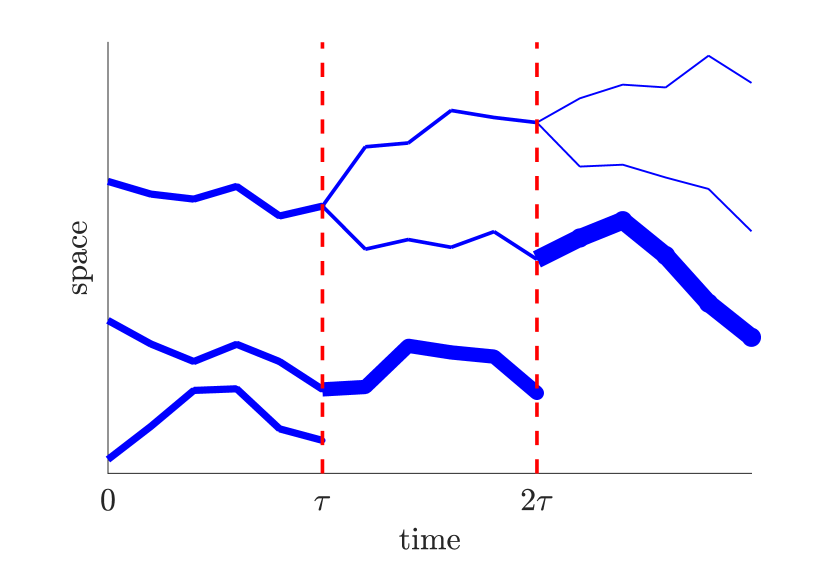
Figure 1: An illustration of splitting and merging of weighted trajectories. Weights are represented by the widths of trajectories. Two splitting and merging steps are shown, in which the top trajectory is split and the bottom trajectories are merged. Trajectory weights are combined with merging and divided with splitting.

The first splitting and merging algorithm was reported in the 1950s and attributed to von Neumann Kahn and Harris (1951). In 1996, Huber and Kim Huber and Kim (1996) modified von Neumann’s original approach by grouping the trajectories into bins and applying splitting and merging in each of the bins separately, thus preserving the bin weights. It was recently shown that WE with fixed bin weights leads to convergent estimatesAristoff (2022); Webber, Aristoff, and Simpson (2020); in contrast, von Neumann’s original method can be unstable in the large time limitAristoff (2022); Webber, Aristoff, and Simpson (2020).

Attention to WE has grown, and the method is now implemented in the widely used WESTPA software package Zwier et al. (2015); Russo et al. (2021) and the more recent wepy package Lotz and Dickson (2020). A Julia language package, used here, is also available, Aristoff et al. (2020). Meanwhile, a growing community of researchers is promoting the method and developing it in different directions Zhang, Jasnow, and Zuckerman (2007); Dickson and Brooks III (2014); Adelman et al. (2011); Zwier, Kaus, and Chong (2011); Abdul-Wahid et al. (2014); Ahn et al. (2021); Ray and Andricioaei (2020); Ray, Stone, and Andricioaei (2021); Ojha et al. (2022).

In modern biochemical applications, WE is often used to estimate the MFPT for a stochastic dynamics to transition from a source state $A$ into a target state $B$ Zuckerman and Chong (2017). In addition, WE has been used to estimate other transition path statistics, including the distribution of reaction times from $A$ to $B$ Zhang, Jasnow, and Zuckerman (2007); Zwier, Kaus, and Chong (2011), the distribution of entry points into $B$ Bhatt and Zuckerman (2011); Dickson and Brooks III (2014), and the characteristics of paths leading from $A$ to $B$ Zhang, Jasnow, and Zuckerman (2007); Adelman et al. (2011). Here, we focus on the estimation of MFPTs, which is a significant and challenging application because the inverse of the MFPT is the reaction rate constant Bhatt, Zhang, and Zuckerman (2010).

Other computational techniques for estimating MFPTs include Markov state models Swope, Pitera, and Suits (2004), forward flux sampling Allen, Warren, and Ten Wolde (2005), adaptive multilevel splitting Cérou and Guyader (2007), exact milestoning Bello-Rivas and Elber (2015); Aristoff, Bello-Rivas, and Elber (2016), non-equilibrium umbrella sampling Warmflash, Bhimalapuram, and Dinner (2007), and transition interface sampling van Erp, Moroni, and Bolhuis (2003). Like WE, these approaches use large numbers of short, unbiased trajectories to compute the MFPT. However, the following combination of features makes WE especially attractive:

• WE only requires simulation of the stochastic model forward in time, never backward. Thus, WE can be applied to a wide variety of stochastic models arising in chemistry Huber and Kim (1996); Donovan et al. (2013) and in other areas, e.g., astronomy Abbot et al. (2021), climate science Finkel et al. (2021a, b), and systems biology Donovan et al. (2013, 2016).

• WE is fully parallelizable over time intervals of length $\tau$ between splitting/merging events Darve and Ryu (2012); Zwier et al. (2015); Russo et al. (2021). Since the trajectories are simulated for the same time interval, the parallellization can be managed simply and efficiently.

• WE provides asymptotically unbiased, convergent estimates in the limit of many time steps for any choice of parameters Zhang, Jasnow, and Zuckerman (2010); Aristoff (2022); Webber, Aristoff, and Simpson (2020).

• WE has been observed to provide better MFPT estimates than estimates from Markov state models Feng et al. (2015) or non-equilibrium umbrella sampling Adelman and Grabe (2013).

Despite progress over the last three decades, theoretical questions about WE have remained unanswered until recently. WE performance is highly dependent on the choice of parameters Zhang, Jasnow, and Zuckerman (2007), including the definition of the bins and the desired number of trajectories in each bin. For a long time it was unclear what the optimal parameter choices would be.

Recent work in the mathematical literature sheds new light on the optimal parameter choices for WE Aristoff (2018); Aristoff and Zuckerman (2020); Aristoff (2022); Webber, Aristoff, and Simpson (2020). The optimal merging coordinate is the local MFPT to $B$ given the current state. The optimal splitting coordinate is the local variance of the MFPT to $B$, given the current state and the time interval $\tau$. There is a theoretical limit on the variance reduction achievable through WE, and bins based on the optimal merging and splitting coordinates ensure the optimal variance in the limit of many trajectories and many time steps.

In this article, we aim to communicate these recent mathematical advances in a brief, accessible way. We identify the optimal splitting and merging coordinates in one- and two-dimensional examples. We propose optimized bins based on these coordinates, which differ from the more traditional bins based on the root mean square displacement (RMSD) to $B$. Our examples show that binning based on the RMSD can give catastrophically wrong results. In such cases, more effective bins are needed, and optimization based on reaction coordinates is helpful.

The rest of the article is organized as follows. Section II discusses the computation of mean first passage times, which is a major problem addressed by WE; Section III introduces the WE method; Section IV identifies the optimal merging and splitting coordinates for WE; Section V recommends variance reduction strategies for WE; and Section VI concludes.

Table 1: Definitions of symbols used in this work.

Symbol	Definition
$X_{t}$	underlying Markovian dynamics
$\beta$	inverse thermal energy ($1/k_{B}T$)
$U$	potential energy
$\tau$	evolution time interval or lag time
$A$	initial (source) set
$B$	target (sink) set
$\rho_{A}$	initial (source) distribution inside $A$
$T_{B}$	first passage time to $B$
$N_{t}$	number of arrivals in $B$ by time $t$
$q$	committor function from $A$ to $B$
$J$	steady-state flux into $B$
$\pi$	steady state of source-sink dynamics
$\langle\rangle$	mean or average for source-sink dynamics
$h$	(flux) discrepancy function
$v^{2}$	(flux) variance function
$\hat{J}_{t}$	WE estimate of steady-state flux up to time $t$
${\tilde{\pi}}$, ${\tilde{h}}$, ${\tilde{v}}$	$\tau\to 0$ limits of $\pi$, $h$, $v^{2}$

II Mean first passage times and the Hill relation

We will study the MFPT of a Markovian stochastic dynamics $X_{t}$ from a source state $A$ to a sink state $B$. In the biochemistry context, $X_{t}$ could represent stochastic molecular dynamics such as Langevin dynamics or constant-energy dynamics generated with a stochastic thermostat. The MFPT could correspond to the characteristic time for folding, binding, or conformational change of a simulated protein.

To define the MFPT precisely, we must specify the distribution of starting points $\rho_{A}$ within the the source state $A$. Different choices of $\rho_{A}$ will lead to different MFPTs, even if $A$ remains the same. The distribution $\rho_{A}$ fully determines the MFPT, which is defined as the averaged length of the trajectories initiated from the source distribution $\rho_{A}$ and absorbed upon reaching $B$.

When computing the MFPT, we “recycle” $X_{t}$ according to the source distribution $\rho_{A}$ upon arrival at the sink state $B$. This means that the location immediately changes from $B$ to $A$, but the time index $t$ continues to increase as usual. We assume that the distribution of trajectories for this source-sink recycling dynamics converges as $t\rightarrow\infty$ to a unique steady-state distribution, denoted by $\pi$.

Under these recycling boundary condition, the Hill relation Hill (2005) expresses the $\mathrm{MFPT}$ as the inverse of the steady-state flux $J$ of $X_{t}$ into $B$. To state this more precisely, write $T_{B}$ for the first passage time to $B$, and $N_{t}$ for the number of arrivals of $X_{t}$ in $B$ by time $t$. The Hill relation then states:

$$\langle T_{B}\rangle_{A} =\textup{ MFPT of }X_{t}\textup{ from }A\textup{ to }B$$ (1)

$$=1/J=\left(\textup{steady-state flux into }B\right)^{-1}$$ (2)

$$=\left(\frac{d}{dt}\langle N_{t}\rangle_{\pi}\right)^{-1}.$$ (3)

Here and elsewhere, we use subscripts to indicate the starting distribution for the dynamics $X_{t}$. Thus, $\langle T_{B}\rangle_{A}$ indicates the mean first passage time when $X_{0}$ is started from $\rho_{A}$, and $\langle N_{t}\rangle_{\pi}$ indicates the mean number of arrivals when $X_{0}$ is started from $\pi$. Equation (2) holds for any $t\geq 0$, since $\pi$ is the steady state.

The application of the Hill relation transforms the computation of a long expected time (the MFPT) into a computation of a small rate (the steady state flux into $B$). This transformation makes it possible, in principle, to compute the MFPT using trajectories with lengths much shorter than the MFPT. Moreover, these short trajectories can be run in parallel to reduce the wall-clock time. Yet, a large number of trajectories are required since the flux can be very small.

Fortunately the Hill relation can be combined with enhanced sampling approaches like WE to help accurately estimate the small flux into $B$. It is necessary that the trajectories approximate the steady-state distribution $\pi$, but this can frequently be attained, because the timescale for relaxation to steady state can be much shorter than the MFPT in problems of interestBen-Ari and Pinsky (2007).

Figure 2 shows a simple system in which the steady-state flux from $A$ into $B$ is small. Like many of the examples to follow, the data in the figure comes from overdamped Langevin (“Brownian”) dynamics

$$\mathop{dX_{t}}=\Bigl{[}\nabla D(X_{t})-\beta D(X_{t})\nabla U(X_{t})\Bigr{]}\mathop{dt}+\sqrt{2D(X_{t})}\mathop{dW_{t}}$$ (4)

associated with the Smoluchowski equation

$$\partial_{t}p(x,t)=\nabla\cdot\Bigl{[}D(x)\Bigl{(}\beta\nabla U(x)p(x,t)+\nabla p(x,t)\Bigr{)}\Bigr{]}.$$ (5)

Here, $\beta>0$ is an inverse temperature constant, $U:\mathbb{R}^{n}\rightarrow\mathbb{R}$ is a scalar potential, $D:\mathbb{R}^{n}\rightarrow\mathbb{R}$ is a diffusion coefficient, ${W}$ is a standard Brownian motion, and $p(x,t)$ is the probability density at location $x$ at time $t$. For simplicity, we assume a dimensionless configurational coordinate $x$, which results in a diffusion coefficient $D$ exhibiting units of inverse time.

For exposition, many of our examples are in one or two spatial dimensions. We emphasize, however, that the WE method and the core mathematical analysis here apply to any Markovian stochastic dynamics in any spatial dimension.

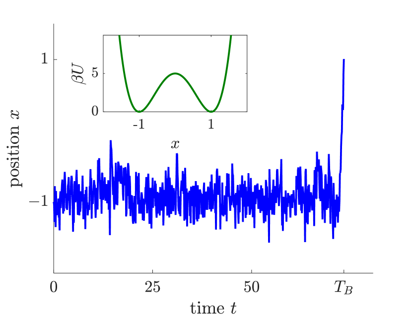
Figure 2: A first passage event out of a local minimum of $U$. After a long waiting period, the first entry into the set $B=\{x>1\}$ occurs at time $T_{B}$. The dynamics satisfies Smoluchowski dynamics (4) with $\beta U(x)=5(x-1)^{2}(x+1)^{2}$ and $D=1/5$ (inverse time units).

The continuous-time Smoluchowski equation needs to be discretized for numerical simulation. Therefore, we assume that $X_{t}$ is evolved as a discrete time series $X_{0},X_{\tau},X_{2\tau},\ldots$, and $X_{t}$ is only recycled when it occupies state $B$ at a multiple of the time interval $\tau$. The difference between discrete- and continuous-time flux into $B$ will be small if $\tau$ is small or the trajectories in $B$ are very slow to escape. We reserve variables $t$ and $\tau$ for the “physical time”, i.e., the time index for the original dynamics $X_{t}$.

III Weighted ensemble: Splitting and merging

Throughout this article we consider a simple version of WE in which the splitting and merging of trajectories are reformulated as resampling Zhang, Jasnow, and Zuckerman (2010); Aristoff and Zuckerman (2020); Aristoff (2022); Webber, Aristoff, and Simpson (2020). For a more general discussion of WE, see the review Zuckerman and Chong (2017). The simple WE algorithm is described below and illustrated in Figure 3.

• Initialization. Select starting points for $N$ trajectories. Assign a weight to each trajectory so that the weights sum to one.

• Resampling. Partition the $N$ trajectories into bins, and select the desired number of copies for each bin, called the allocation. The bins are simply groupings of the trajectories, and they may change in time. The allocations are positive integers which may change with time but are assumed to always sum to $N$.

  Next, resample trajectories within each bin with probabilities proportional to the weights, and divide the total weight in each bin evenly among the resampled trajectories Aristoff (2022).

• Dynamics. Evolve the trajectories independently for time $\tau$ according to the underlying dynamics.

• Convergence. Repeat steps 2-3 as long as desired or possible. Estimate the steady-state flux $J$ using the average WE probability flux entering $B$ from the burn-in time $t_{0}$ to the final time $t$. That is,

  $$\hat{J}_{t}=\frac{\textup{Total WE weight entering $B$}}{t-t_{0}},$$ (6)

  where $t-t_{0}$ is the physical time of simulations following the burn-in. The estimate for $J$ in turn yields a MFPT estimate via the Hill relation (2).

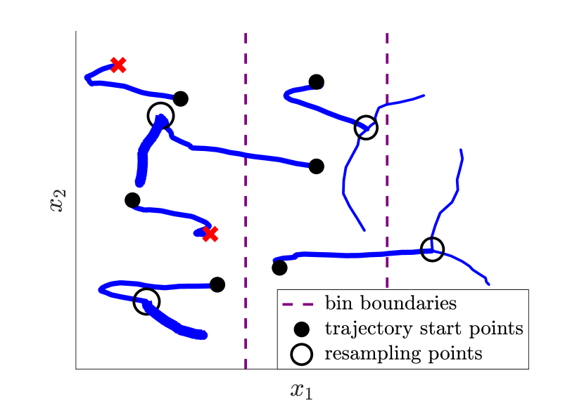
Figure 3: An example of WE evolution and resampling. Pictured are $6$ WE trajectories, which undergo evolution, resampling, and another round of evolution. The bins are based on the coordinate $x_{1}$. During evolution steps, the trajectories travel between bins, and the resampling enforces $2$ copies in each bin. Circles indicate trajectories that are continued and possibly replicated during resampling; crosses indicate trajectories that are pruned during resampling. Trajectory weight is represented by line width.

The crucial step in WE is the resampling step, which leads to the splitting and merging of trajectories. Splitting is the dynamics of replicating trajectories that are “valuable,” while merging is the act of combining trajectories that are “similar.” Splitting improves the accuracy of the flux estimates, especially when the duplicated trajectories are expected to make large contributions to the future flux. With repeated splitting, merging is needed to limit the number of trajectories.

Although splitting and merging are traditionally applied separately, in the simple WE algorithm above these steps are combined via resamplingZhang, Jasnow, and Zuckerman (2010). In each bin, trajectories are resampled with probabilities proportional to their weights, with the resampled trajectories each receiving an equal proportion of the bin weight. Resampling is easier to formulate and implement than the traditional splitting and merging. Moreover, resampling is optimal when trajectories within a given bin are, except for their weights, indistinguishable Darve and Ryu (2012).

Splitting and merging must be balanced, and a main contribution of our recent work Aristoff (2018); Aristoff and Zuckerman (2020); Aristoff (2022); Webber, Aristoff, and Simpson (2020) has been identifying the regions of state space in which splitting or merging should be promoted. Identifying such regions naturally leads to variance reduction strategies. We discuss these developments in Sections IV and V.

Given sufficient resources, the WE method terminates when the estimated flux converges to a near-constant value. However, if steady state cannot be reached during the available simulation time, enhanced methods for WE initialization are needed. For example, incorporating an appropriate burn-in time $t_{0}>0$ can reduce transient relaxation effects Adhikari et al. (2019), and adjusting the initial weights can also improve convergence Copperman and Zuckerman (2020).

WE can be used to estimate other transition path statistics in addition to the steady-state flux. For instance, the WE-generated paths and the associated weights can be used to estimate the distribution of reaction times (i.e., event durations) and the distribution of mechanistic pathways Zhang, Jasnow, and Zuckerman (2007). See Appendix .1 for a discussion.

IV Optimal splitting and merging coordinates

Recent mathematical analysis has revealed the existence of optimal reaction coordinates for merging and splitting in WE Aristoff and Zuckerman (2020); Webber, Aristoff, and Simpson (2020); Aristoff (2022). Sections IV.1 and IV.2 provide general formulas for these optimal reaction coordinates that assume no particular type of dynamics or dimensionality, while Section IV.3 provides more explicit formulas that hold for the Smoluchowski dynamics.

IV.1 Optimal merging and splitting coordinates

Optimal merging. Merging trajectories, i.e., pruning some members of a chosen set, is least harmful and most beneficial when the groups of trajectories to be merged are in some sense “similar.” For the MFPT problem, the scalar reaction coordinate that characterizes this similarity is the flux discrepancy function Aristoff and Zuckerman (2020)

$$h(x)=\lim_{t\to\infty}\left[\left\langle N_{t}\right\rangle_{x}-\left\langle N_{t}\right\rangle_{\pi}\right].$$ (7)

$N_{t}$ counts the total number of crossings into $B$ at times $s=\tau,2\tau,\ldots,t$. Thus, $h(x)$ is the difference in expected future flux between trajectories started at the particular point $x$ and trajectories started from the steady-state distribution $\pi$. Since trajectories with similar $h$ values make similar expected contributions to the flux estimate, merging trajectories with similar $h$ values is appropriate Aristoff and Zuckerman (2020); Aristoff (2022).

Using the Hill relation, the flux discrepancy function can be rewritten in terms of MFPTs initiated from different starting distributions. As shown in Appendix .2,

$$h(x)=\frac{\langle T_{B}\rangle_{\pi}-\langle T_{B}\rangle_{x}}{\langle T_{B}\rangle_{A}},$$ (8)

where we recall $T_{B}$ is the first passage time into $B$ excluding time $t=0$. Equation (8) allows us to reinterpret the optimal merging function as a normalized difference between the local MFPT to $B$ starting from $x$ and the MFPT for trajectories initiated from the steady state $\pi$. Identity (8) holds independently of both the dimension and the type of Markovian dynamics. It shows that the flux discrepancy function and the local MFPT are equivalent optimal coordinates for merging.

Optimal splitting. Splitting – the duplication of certain WE trajectories – increases local sampling and is of high benefit in regions that are important for the flux computation. We now introduce the scalar reaction coordinate that describes optimal splitting behavior, the flux variance function Aristoff and Zuckerman (2020)

$$v(x)^{2}=\tau^{-1}\textup{Var}_{x}\bigl{[}h_{0}(X_{\tau})\bigr{]},$$ (9)

where $h_{0}$ is a version of the discrepancy function that counts flux at time $t=0$, i.e., $h_{0}(x)=\mathds{1}_{B}(x)+h(x)$, and $\textup{Var}_{x}$ denotes variance for the source-sink dynamics started at $x$. The flux variance function quantifies the variation in the expected flux over a time interval $\tau$ for trajectories initiated at $x$.

As a heuristic strategy, a favorable allocation should satisfy Aristoff (2018); Aristoff and Zuckerman (2020); Aristoff (2022)

$$\#\textup{ trajectories near }x\propto\pi(x)v(x).$$ (10)

Allocating in this way minimizes the future contribution to the flux variance, assuming that WE is in steady state Aristoff (2018); Aristoff and Zuckerman (2020); Aristoff (2022). We refer to this as the optimal allocation distribution and provide an intuitive derivation in Appendix .3.

As a more rigorous mathematical result, the following establishes the optimality of $h$ and $v$ as WE reaction coordinates.

Theorem Webber, Aristoff, and Simpson (2020). If the recycled dynamics $X_{t}$ is geometrically ergodic, then the WE method satisfies the following:

1. For any choice of bins and allocations, the WE flux estimate $\hat{J}_{t}$ given in (6) converges with probability one to the inverse MFPT,

   $$\lim_{t\rightarrow\infty}\hat{J}_{t}=\frac{1}{\langle T_{B}\rangle_{A}}.$$ (11)

2. For any $\epsilon>0$ and any choice of bins and allocations, the WE variance satisfies

   $$\textup{Var}\,\hat{J}_{t}\geq\frac{1-\epsilon}{Nt}\Bigl{(}\int v(x)\pi(x)\mathop{dx}\Bigr{)}^{2}$$ (12)

   when $t$ is sufficiently large.

3. For any $\epsilon>0$, if the bins are sufficiently small rectangles in $h$ and $v$ coordinates and if the allocation for each bin is proportional to $\int_{\textup{bin}}v(x)\pi(x)\mathop{dx}$, the WE variance satisfies

   $$\textup{Var}\,\hat{J}_{t}\leq\frac{1+\epsilon}{Nt}\Bigl{(}\int v(x)\pi(x)\mathop{dx}\Bigr{)}^{2}$$ (13)

   for sufficiently large $t$ and $N$. ∎

The theorem holds regardless of dimension, temperature, time $\tau$, and type of Markovian dynamics. It highlights the following WE strategy that is optimal in the limit of large $N$ and $t$: trajectories with similar $h$ and $v$ values are merged, while splitting enforces $\textup{Const}\times\pi(x)v(x)$ trajectories near $x$. The theorem supports the interpretation (10) of $\pi(x)v(x)$ as the optimal distribution for trajectory allocation.

IV.2 Maximum gain of WE over direct dynamics

The above mathematical theory enables a quantitative comparison between WE and direct Monte Carlo sampling of first-passage events. Here, we define direct Monte Carlo as independent trajectories without any splitting or merging.

Assuming that trajectories are started from the steady state $\pi$, the direct Monte Carlo variance with $N$ trajectories can be written Webber, Aristoff, and Simpson (2020)

$$\frac{1}{Nt}\int v(x)^{2}\pi(x)\mathop{dx}.$$ (14)

This formula reveals that the flux variance function $v^{2}$ is intrinsic to direct Monte Carlo dynamics as well as WE dynamics, since $v^{2}$ quantifies the variance in the flux estimates as trajectories are evolved forward over a time interval $\tau$. Dividing (14) by (13), the ratio of direct Monte Carlo variance to optimal WE variance is then Webber, Aristoff, and Simpson (2020)

$$\begin{split}&\textup{Optimal gain over direct Monte Carlo}\\ &\quad=\frac{\int v^{2}(x)\pi(x)\,dx}{\left(\int v(x)\pi(x)\,dx\right)^{2}}.\end{split}$$ (15)

This ratio quantifies the maximal possible variance reduction achievable by WE in the large time limit, for any number of trajectories.

The optimal gain over direct Monte Carlo has important implications. Analytical and numerical investigation of this quantity can yield insight into how much benefit is possible from using WE. Additionally, knowing the optimal gain over direct Monte Carlo as a reference enables quantitative comparisons of different WE binning strategies against the theoretically optimal performance.

IV.3 Optimal WE for one-dimensional Smoluchowski dynamics

To make the preceding theory more explicit, we consider Smoluchowski (overdamped Langevin) dynamics in a one-dimensional setting with a source state $A=\{x\leq a\}$ and a sink state $B=\{x\geq b\}$, where $a<b$. The recycling distribution is a delta function at the edge $a$ of $A$, i.e., $\rho_{A}=\delta(x-a)$. We consider the continuous-time limit, $\tau\rightarrow 0$, which leads to simpler, more interpretable mathematical expressions.

In the limit $\tau\rightarrow 0$, the dynamics $X_{t}$ is observed at all times and recycling occurs immediately upon entry into $B$. The steady-state distribution ${\tilde{\pi}}$ can be calculated using the relation Lu and Nolen (2015)

$${\tilde{\pi}}(x)\propto[1-{\tilde{q}}(x)]e^{-\beta U(x)}.$$ (16)

Here, ${\tilde{q}}$ is the committor function, the probability for $X_{t}$ to reach $B$ before $A$ starting from $x$, which is given by Gardiner et al. (1985)

$${\tilde{q}}(x)=\begin{cases}0&x\leq a,\\ \dfrac{\int_{a}^{x}e^{\beta U(y)}/D(y)\,dy}{\int_{a}^{b}e^{\beta U(y)}/D(y)\,dy}&x<a<b,\\ 1&x\geq b.\end{cases}$$ (17)

Using (16) and (17), the steady-state distribution is supported on $\{x<b\}$, and it satisfies

$${\tilde{\pi}}(x)\propto e^{-\beta U(x)}\int_{\max\{x,a\}}^{b}\frac{e^{\beta U(y)}}{D(y)}\,dy.$$ (18)

Compared to the Boltzmann density $\propto e^{-\beta U(x)}$, the steady-state density $\tilde{\pi}$ removes mass from the regions near $B$ due to the recycling of trajectories. See Figure 4 for an illustration.

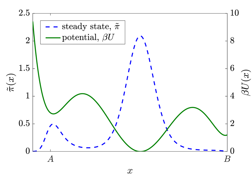
Figure 4: The steady state of the source-sink dynamics. Plotted is the steady state ${\tilde{\pi}}$ of the Smoluchowski dynamics with recycling from $B$ to $A$, a diffusion coefficient $D=1$, and $\beta=4$. In this and subsequent figures, $U(x)=5(x-1)^{2}x^{2}(x+1)^{2}+0.5x^{2}-0.2x$.

The flux discrepancy function $h=h_{\tau}$ and the flux variance function $v=v_{\tau}$ depend implicitly on the evolution interval $\tau$, and they converge to well-defined limits as $\tau\rightarrow 0$:

$${\tilde{h}}(x)=\lim_{\tau\to 0}h_{\tau}(x),\qquad{\tilde{v}}^{2}(x)=\lim_{\tau\to 0}v_{\tau}(x)^{2}.$$ (19)

As a result of (8), the discrepancy function ${\tilde{h}}$ satisfies

$$\tilde{h}(x)=\frac{\langle\tilde{T}_{B}\rangle_{\tilde{\pi}}-\langle\tilde{T}_{B}\rangle_{x}}{\langle\tilde{T}_{B}\rangle_{A}}.$$ (20)

Here, $\tilde{T}_{B}$ is the exact MFPT function to the target state $B$, which is given for $x\leq b$ by Gardiner et al. (1985)

$$\langle{\tilde{T}}_{B}\rangle_{x}=\int_{x}^{b}\frac{e^{\beta U(z)}}{D(z)}\int_{-\infty}^{z}e^{-\beta U(y)}\,dy\,dz.$$ (21)

The variance function ${\tilde{v}}$ satisfies the relations

$${\tilde{v}}^{2}(x)=\lim_{\tau\rightarrow 0}\frac{\textup{Var}_{x}\bigl{[}\tilde{h}(X_{\tau})\bigr{]}}{\tau}=2D(x)\Bigl{|}\frac{d}{dx}\tilde{h}(x)\Bigr{|}^{2},$$ (22)

where the first equality follows from the definition (9) and the second equality comes from applying Itô’s lemma Gardiner et al. (1985). Formula (22) suggests that there should be more splitting in regions of high $\tilde{h}$ variability, or, equivalently, high variability in the local MFPT $\langle\tilde{T}_{B}\rangle_{x}$.

Note that the committor $\tilde{q}$ is usually understood to be the relevant coordinate for computing the MFPT and similar problems Ma, Elber, and Makarov (2020). We have shown, however, that two different scalar coordinates, namely $\tilde{h}$ and $\tilde{v}^{2}$, are the relevant ones for splitting and merging in the context of WE simulation. The difference between these coordinates is exhibited by a model problem with an asymmetric two-barrier system in Figure 5. For this problem, the committor ${\tilde{q}}$ would not be an ideal reaction coordinate since it poorly resolves the largest barrier on the forward path from $A$ to $B$. In contrast, ${\tilde{h}}$ and ${\tilde{v}}$ resolve the largest forward barrier, making them appropriate for WE.

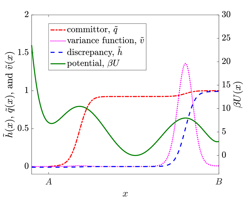
Figure 5: The ideal reaction coordinates for WE. Plotted are the discrepancy function ${\tilde{h}}$ the committor ${\tilde{q}}$ and the variance function ${\tilde{v}}$ for the Smoluchowski dynamics with recycling from $B$ to $A$, a diffusion coefficient $D=1$, and $\beta=10$.

Lastly, a simple formula for the optimal WE allocation holds in the low-temperature limit as $\beta\rightarrow\infty$. Assume that the largest energy increase on the forward path to $B$ occurs over the interval $[x_{-},x_{+}]$, i.e.,

$$\Delta U=U(x_{+})-U(x_{-})=\max_{a\leq y\leq b,\,x<y}(U(y)-U(x)).$$ (23)

Note that the interval $[x_{-},x_{+}]$ can include multiple energy barriers. Then, as $\beta\rightarrow\infty$, an application of Laplace’s method (see Appendix .4) yields

$$\frac{{\tilde{\pi}}(x){\tilde{v}}(x)}{\int{\tilde{\pi}}(y){\tilde{v}}(y)\mathop{dy}}\to\begin{cases}0&x\leq x_{-},\\ \dfrac{D^{-1/2}(x)}{\int_{x_{-}}^{x_{+}}D^{-1/2}(y)\mathop{dy}}&x_{-}<x<x_{+},\\ 0&x\geq x_{+}.\end{cases}$$ (24)

Thus, the optimal allocation is proportional to $1/\sqrt{D}$ over the interval $[x_{-},x_{+}]$, and it is vanishingly small elsewhere as illustrated in Figure 6.

In the low-temperature limit $\beta\rightarrow\infty$, the optimal gain over direct Monte Carlo sampling grows exponentially with the size of the largest energy increase (see Appendix .4):

$$\textup{Gain over direct Monte Carlo}\\ \overset{\beta\to\infty}{\sim}\frac{\pi/\beta}{\left(\int_{x_{-}}^{x_{+}}\sqrt{D(x_{+})/D(x)}\,dx\right)^{2}}\frac{e^{\beta\Delta U}}{\sqrt{|U^{\prime\prime}(x_{-})U^{\prime\prime}(x_{+})|}}.$$ (25)

This provides a formal explanation of earlier numerical findings Zhang, Jasnow, and Zuckerman (2007); DeGrave et al. (2018) that WE’s advantage over direct Monte Carlo grows dramatically as $\beta\Delta U$ increases.

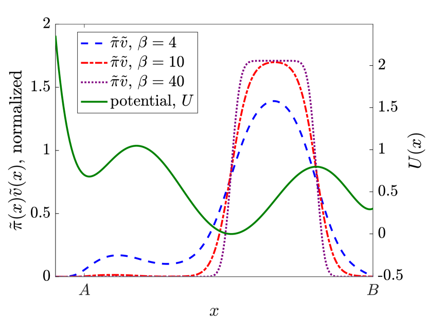
Figure 6: The optimal allocation distribution at low temperature. Plotted is the optimal allocation distribution ${\tilde{\pi}}{\tilde{v}}$ for the Smoluchowski dynamics with recycling from $B$ to $A$ and with increasing values of $\beta$ when $D=1$. In the limit $\beta\rightarrow\infty$, the optimal allocation distribution is constant along the interval of largest energy increase; see (24).

V A principled WE strategy

The theoretical results above can serve as guidelines for optimizing WE. For example, we describe one principled WE strategy called “MFPT binning” in Section V.1, and we compare MFPT binning to a more traditional WE binning strategy in Section V.2.

V.1 MFPT binning

From the theory in Section IV.1, merging has a low cost among trajectories with similar $h$ values. This motivates the following MFPT binning strategy in which bins are comprised of similar $h$ values Aristoff and Zuckerman (2020); Aristoff (2022), or equivalently based on (8), similar values of the local MFPT to $B$:

• Define the bins to be intervals in the $h$ coordinate. If there are $K$ bins, choose the endpoints $h_{0}<h_{1}<\ldots<h_{K}$ such that

  $$\int_{h_{k}\leq h(x)\leq h_{k+1}}\pi(x)v(x)dx=\text{Const.}$$ (26)

• Allocate trajectories uniformly among these $K$ bins, so that approximately $N/K$ trajectories are assigned to each bin.

This approach agrees with strategy (10) while also satisfying the traditional WE rule of keeping the number of trajectories per bin nearly constant. See Figure 7 for an illustration.

The MFPT binning strategy is similar to the one described in Section IV.1, which attains the lowest possible variance in the limit of many trajectories and time steps. However, instead of bins that are rectangles in $h$ and $v$ coordinates, we define bins as intervals of $h$ values alone. This alteration still performs well in our model problem in Section V.2, even with a small number of trajectories ($100$–$1000$) and just a few bins ($5$–$10$).

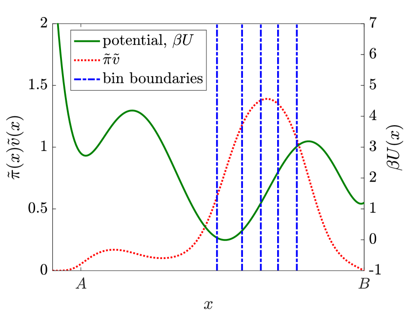
Figure 7: Illustration of MFPT binning strategy. Pictured are $6$ bins, with dividing surfaces between bins indicated by the vertical lines. Bin boundaries are chosen to make the integral of ${\tilde{\pi}}{\tilde{v}}$ within each bin constant. Here, $D=1$ and $\beta=4$. In higher-dimensional spaces, bin boundaries would be level sets of $h$ as in Figure 8.

The MFPT binning strategy requires an approximation to the flux discrepancy function $h$ and flux variance function $v$. Strategies for estimating the functions will be explored in future work. We note that even crude estimates of $h$ and $v$ may be helpful, compared to naive or ad-hoc binning strategies, and WE remains unbiased regardless of the approximation quality of $h$ and $v$. As a concrete strategy Aristoff and Zuckerman (2020), initial simulations can be performed, and discrete Markov state models Chodera and Noé (2014) (MSMs) can be used to approximate $h$ and $v$ based on the relationships to the MFPT described in Section IV.

In contrast to this MFPT binning strategy, the most common WE approach Zuckerman and Chong (2017) involves bins defined using root mean square displacement (RMSD) to $B$ in some feature space, with the same number of trajectories allocated to each bin. This approach would be optimal if the dynamics in the RMSD coordinate were well-described by the one-dimensional Smoluchowsi equation (5) with large $\beta$ and constant $D$; see Section IV.3 and Figure 5. However, the RMSD coordinate rarely behaves in this way for complex systems, and our results below show that RMSD binning can catastrophically fail when the RMSD coordinate is very different from the MFPT.

V.2 Numerical comparison

In this section, we numerically compare two strategies for binning and allocation within WE:

1. The MFPT binning strategy discussed in Section V.1.

2. Traditional WE bins based on RMSD to $B$ with allocations proportional to $\int_{\textup{bin}}v(x)\pi(x)\mathop{dx}$.

In both strategies, the allocations enforce the heuristic (10) of having $\mathrel{\vbox{ \offinterlineskip\halign{\hfil$#$\cr\propto\cr\kern 2.0pt\cr\sim\cr\kern-2.0pt\cr}}}\pi(x)v(x)$ trajectories near $x$, which is derived mathematically in Section IV.

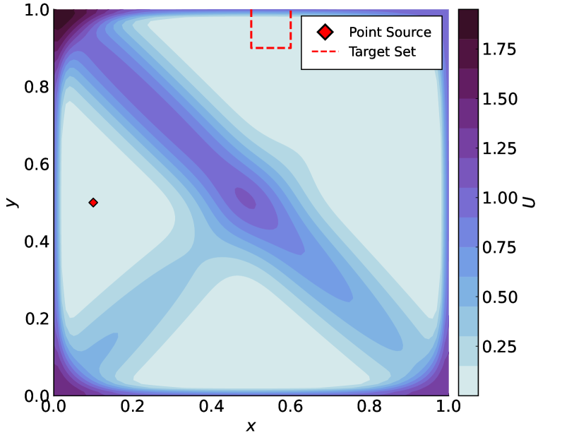
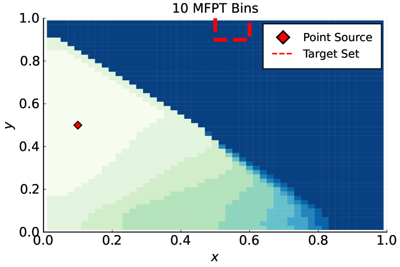
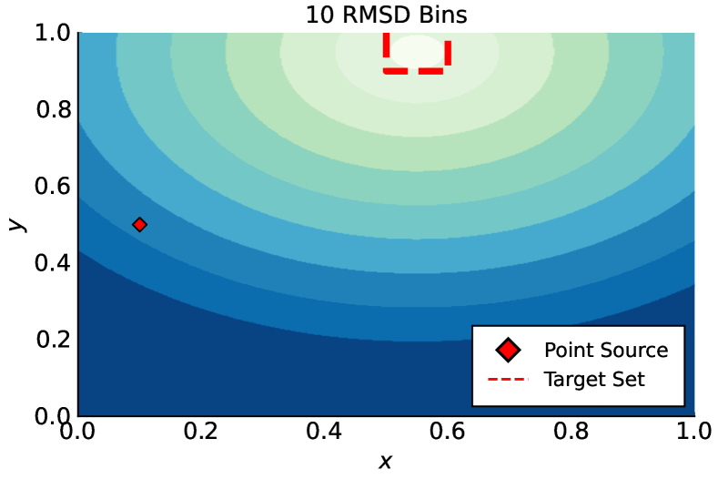
Figure 8: Different binning strategies in a challenging two-dimensional model. Pictured are the potential $U$ (top), MFPT bins (middle), and RMSD bins (bottom), with the source $A$ depicted as a filled dot and the sink $B$ depicted as a dashed rectangle. Different shades indicate different bins. The model is fully specified in Appendix .5: see the potential (50).

We will apply these WE strategies to the two-dimensional Smoluchowski model system pictured in Figure 8, with full specifications in Appendix .5. We begin our study of this model by constructing a fine-grained MSM approximation of functions $\pi$, $h$, and $v$. Next, we use these approximations to construct the MFPT bins in Figure 8. Observe that the MFPT bins resolve the largest energy barriers on the forward path from $A$ to $B$, whereas the RMSD bins have concentric circle bin boundaries that do not account for the energy landscape at all. See Appendix .5 for further bin construction details. These computations were performed using Aristoff et al. (2020).

To evaluate the precision – and hence, efficiency – of the flux estimates from MFPT and RMSD binning, we define a compute-cost-independent variance constant:

$$\begin{split}\textup{Variance Constant}=Nt\times\textup{Var}\left(\hat{J}_{t}\right).\end{split}$$ (27)

Here, the variance of the empirical WE flux has been scaled to account for total simulation cost $Nt$. The variance constants for MFPT and RMSD binning are compared in Figure 9. The figure also shows estimates of the optimal WE variance constant $(\int\pi v)^{2}$ from the fine-grained MSM model (see equation (LABEL:eq:opt_var_const)), as well as the variance constant for direct Monte Carlo, without any splitting or merging. We used $N=10^{4}$ trajectories and averaged over $10^{2}$ independent runs to produce these variance constants.

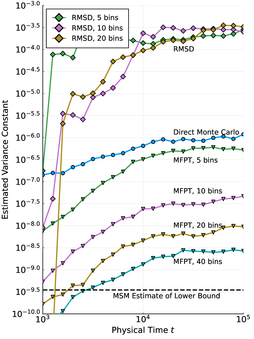
Figure 9: Comparison of binning strategies for MFPT estimation. Estimates of the rescaled variance constant (27) are plotted for MFPT and RMSD binning strategies for the two-dimensional problem depicted in Fig. 8. For this problem, the flux value is approximately $10^{-6}$.

Figure 9 reveals a dramatic difference between MFPT and RMSD binning. RMSD binning leads to worse-quality results than direct Monte Carlo simulation for this non-trivial model, for any number of bins. Meanwhile, MFPT binning leads to a major improvement over direct Monte Carlo simulation, particularly when the number of bins is large ($20$–$40$ bins). With only $5$ bins, we see a modest gain with the MFPT binning strategy. Increasing the number of bins with MFPT binning systematically improves the output such that with $40$ bins, we are within an order of magnitude of the estimated optimal constant. This is two and a half orders of magnitude of improvement over direct Monte Carlo.

To encourage a fair comparison, we have applied the optimal allocation rule (10) to both MFPT and RMSD binning. However, analogous tests (not pictured) show that RMSD binning performs even worse with uniform allocations, leading to higher variance constants. Our MFPT binning method here also outperformed related strategies in our earlier work Aristoff and Zuckerman (2020).

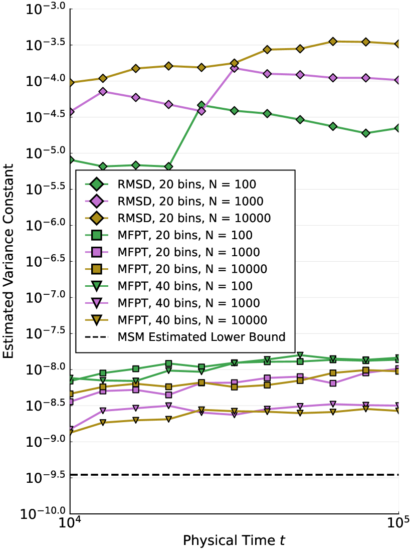
Figure 10: Variance constants for different numbers of trajectories.

Lastly, the data in Figure 9 was generated using $N=10^{4}$ trajectories, which may exceed the computational resources available for problems of interest. Figure 10 presents comparisons for $10^{2}$, $10^{3}$, and $10^{4}$ trajectories, indicating that the variance constant typically has no more than an order of magnitude in variability. In particular, for the MFPT bins the results for $10^{3}$ trajectories are nearly indistinguishable from those obtained with $10^{4}$ trajectories.

VI Conclusion

This work has attempted to assemble, expand upon, and make accessible to a chemical physics audience, recent mathematical results of fundamental importance to weighted ensemble (WE) simulation. The mathematical theory exposes the fundamental capabilities of WE and guiding principles behind WE optimization. It leads to the identification of optimal reaction coordinates for merging and splitting. The theory also identifies the minimal possible variance for WE in the limit of many trajectories and time steps, and we demonstrate a simple binning strategy for approaching that optimum that works well in a two-dimensional model problem. Testing these approaches in complex systems will be pursued in future work.

To illustrate the mathematical theory in a physically intuitive way, explicit formulas were derived for the optimal coordinates and optimal WE variance in the case of the Smoluchowski dynamics (5) in one dimension. These formulas, presented for the first time here, demonstrate that the variance reduction from WE can be exponentially large in the size of the largest forward energy barrier from $A$ to $B$.

The mathematical theory is important because it enables principled variance reduction strategies for WE. Here, we have proposed and tested one such variance reduction strategy, called MFPT binning. After pilot runs that estimate $h$ and $v$ (or equivalently, the local MFPT to $B$ and its variance), this strategy defines the bins to be intervals in the $h$ coordinate, chosen in a way that optimizes the variance. In a model problem, MFPT binning significantly outperforms a naive WE approach that constructs bins using the RMSD to $B$, and these results remain robust even for relatively small $N$.

Appendix

.1 Computing other statistics using WE

WE can be used to compute other statistics, in addition to the MFPT from $A$ to $B$. Namely, any integral $\int f(x)\pi(x)dx$ involving an observable $f$ can be estimated using $N$ WE trajectories. In the long time limit, the trajectories satisfy

$$\int f(x)\pi(x)dx=\lim_{t\rightarrow\infty}\frac{1}{t}\sum_{s=1}^{t}\sum_{i=1}^{N}w_{s\tau}^{i}f(\xi_{s\tau}^{i}),$$ (28)

where $(\xi_{t}^{i},w_{t}^{i})_{1\leq i\leq N}$ denotes the position and weight of trajectory $i$ at time $t$. Therefore, as a practical estimator, we can terminate the simulations at a finite time $t$ and approximate

$$\int f(x)\pi(x)dx\approx\frac{1}{t-t_{0}}\sum_{s=t_{0}}^{t}\sum_{i=1}^{N}w_{s\tau}^{i}f(\xi_{s\tau}^{i}),$$ (29)

where $t_{0}>0$ is a suitable burn-in time. Here we have assumed $f$ is recorded only at $\tau$ intervals, although WE permits saving points more frequently.

The estimator (29) is readily extended to history-dependent observables, such as transition-path times or mechanistic pathways from $A$ to $B$. This requires defining the trajectories as paths starting from $A$, which are recycled upon reaching $B$, and defining $\pi$ as a stationary measure on path space. The recent mathematical literature Aristoff (2018); Aristoff and Zuckerman (2020); Aristoff (2022); Webber, Aristoff, and Simpson (2020) provides a set of error bounds and convergence guarantees for the estimator (29).

.2 Relationship between flux discrepancy and MFPT

To establish the relationship

$$\lim_{t\to\infty}\left[\left\langle N_{t}\right\rangle_{x}-\left\langle N_{t}\right\rangle_{\pi}\right]=\frac{\langle T_{B}\rangle_{\pi}-\langle T_{B}\rangle_{x}}{\langle T_{B}\rangle_{A}},$$ (30)

we first introduce the following terminology:

• $T_{B}^{x}$ is the first passage time into $B$ for a dynamics started at $X_{0}=x$.

• $T_{B}^{\pi}$ is the first passage time into $B$ for a dynamics started at $X_{0}\sim\pi$, i.e., started at a point chosen randomly from the steady-state distribution.

• $N_{t}^{A}$ is the number of arrivals into $B$ by time $t$ for a dynamics started at $X_{0}\sim\rho_{A}$.

Next we recall the renewal theorem from classical probability Feller (2008), which states that for any $s>0$,

$$\lim_{t\rightarrow\infty}\left[\langle N_{t}^{A}\rangle-\langle N_{t-s}^{A}\rangle\right]=\frac{s}{\langle T_{B}\rangle_{A}}.$$ (31)

Lastly, we verify

$$\lim_{t\to\infty}\left[\left\langle N_{t}\right\rangle_{x}-\left\langle N_{t}\right\rangle_{\pi}\right]$$ (32)

$$=\lim_{t\to\infty}\left[\left\langle N_{t-T_{B}^{x}}^{A}\right\rangle-\left\langle N_{t-T_{B}^{\pi}}^{A}\right\rangle\right]$$ (33)

$$=\lim_{t\rightarrow\infty}\left[\left\langle N_{t}^{A}\right\rangle-\left\langle N_{t-T_{B}^{\pi}}^{A}\right\rangle\right]-\lim_{t\to\infty}\left[\left\langle N_{t}^{A}\right\rangle-\left\langle N_{t-T_{B}^{x}}^{A}\right\rangle\right]$$ (34)

$$=\frac{\langle T_{B}^{\pi}\rangle-\langle T_{B}^{x}\rangle}{\langle T_{B}\rangle_{A}},$$ (35)

where we have applied the renewal theorem after conditioning on $s=T_{B}^{\pi}$ and $s=T_{B}^{x}$.

.3 Derivation of optimal allocation rule

In this section we provide an intuitive derivation of the optimal allocation rule

$$\#\textup{ trajectories near }x\propto\pi(x)v(x).$$ (36)

We introduce the following notation:

• $\textup{weight}_{\textup{bin}}$ and $\textup{alloc}_{\textup{bin}}$ indicate a bin weight and bin allocation.

• $\langle\rangle_{\textup{bin}}$ and $\textup{Var}_{\textup{bin}}$ denote the mean and variance with respect to the weighted trajectory distribution in a bin, so $\textup{Var}_{\textup{bin}}(f)=\langle f^{2}\rangle_{\textup{bin}}-\langle f\rangle_{\textup{bin}}^{2}$.

• Finally, $\langle\rangle_{t}$ denotes the average over the WE ensemble up to time $t$.

Then the following variance formula Aristoff (2022); Webber, Aristoff, and Simpson (2020) holds in the limit as $t\rightarrow\infty$:

$$t\textup{Var}(\hat{J}_{t})\sim$$

$$\left\langle\sum_{\textup{bins}}\frac{\textup{weight}_{\textup{bin}}^{2}}{\textup{alloc}_{\textup{bin}}}\left[\textup{Var}_{\textup{bin}}(h)+\textup{Var}_{\textup{bin}}(v)+\langle v\rangle_{\textup{bin}}^{2}\right]\right\rangle_{t}.$$ (37)

We consider a greedy minimization strategy Aristoff and Zuckerman (2020); Aristoff (2022) for minimizing the variance formula (37). The variance terms $\textup{Var}_{\textup{bin}}(h)$ and $\textup{Var}_{\textup{bin}}(v)$ are minimized by choosing bins in which $h$ and $v$ values are nearly constant. The other term, namely,

$$\frac{\textup{weight}_{\textup{bin}}^{2}}{\textup{alloc}_{\textup{bin}}}\langle v\rangle_{\textup{bin}}^{2},$$

is minimized when the allocation is chosen using Aristoff (2018); Aristoff and Zuckerman (2020); Aristoff (2022)

$$\textup{alloc}_{\textup{bin}}\mathrel{\vbox{ \offinterlineskip\halign{\hfil$#$\cr\propto\cr\kern 2.0pt\cr\sim\cr\kern-2.0pt\cr}}}\textup{weight}_{\textup{bin}}\times\langle v\rangle_{\textup{bin}},$$ (38)

which reduces to (36) in the limit of many trajectories.

.4 Low temperature limit

Here we derive the optimal splitting and merging coordinates in the low-temperature limit $\beta\rightarrow\infty$. First, we combine the expression for the steady state

$${\tilde{\pi}}(x)\propto e^{-\beta U(x)}\int_{\max\{x,a\}}^{b}\frac{e^{\beta U(y)}\mathop{dy}}{D(y)}$$ (39)

with the expression for the flux variance function

$$\tilde{v}(x)=\frac{\sqrt{2}e^{\beta U(x)}}{D(x)^{1/2}\langle\tilde{T}_{B}\rangle_{A}}\int_{-\infty}^{x}\frac{\mathop{dy}}{e^{\beta U(y)}},$$ (40)

to obtain the optimal allocation rule

$${\tilde{\pi}}(x){\tilde{v}}(x)\propto\frac{1}{D(x)^{1/2}}\int_{\max\{x,a\}}^{b}\frac{e^{\beta U(y)}\mathop{dy}}{D(y)}\int_{-\infty}^{x}\frac{\mathop{dy}}{e^{\beta U(y)}}.$$ (41)

Next, we assume the pair of points $(x_{-},x_{+})$ is the unique solution to the maximization

$$\max_{a\leq y\leq b,\,x<y}(U(y)-U(x)),$$ (42)

and $U^{\prime\prime}(x_{+})<0<U^{\prime\prime}(x_{-})$. Using Laplace’s method Bender and Orszag (1999) on (41) we obtain, for any $x_{-}<x<x_{+}$,

$$\frac{1}{D(x)^{1/2}}\int_{\max\{x,a\}}^{b}\frac{e^{\beta U(y)}\mathop{dy}}{D(y)}\int_{-\infty}^{x}\frac{\mathop{dy}}{e^{\beta U(y)}}\\ \stackrel{{\scriptstyle\beta\rightarrow\infty}}{{\sim}}\frac{C}{D(x)^{1/2}}\frac{e^{\beta U(x_{+})}}{\beta e^{\beta U(x_{-})}},$$ (43)

where the prefactor $C$ is explicitly

$$C=\frac{2\pi}{D(x_{+})U^{\prime\prime}(x_{-})^{1/2}|U^{\prime\prime}(x_{+})|^{1/2}}.$$ (44)

For $x$ outside of the interval $[x_{-},x_{+}]$, Laplace’s method dictates that the optimal allocation $\pi(x)v(x)$ is exponentially smaller as $\beta\rightarrow\infty$, whence we recover the optimal allocation (24).

From the above calculations, we find that the optimal gain from using WE takes the form

$$\textup{Gain over direct Monte Carlo}=\frac{QR}{S^{2}},$$ (45)

where

$$Q =\int_{-\infty}^{b}\frac{e^{\beta U(x)}}{D(x)}\int_{\max\{x,a\}}^{b}\frac{e^{\beta U(y)}\mathop{dy}}{D(y)}\Bigl{(}\int_{-\infty}^{x}\frac{\mathop{dy}}{e^{\beta U(y)}}\Bigr{)}^{2}\mathop{dx},$$ (46)

$$R =\int_{-\infty}^{b}e^{-\beta U(x)}\int_{\max\{x,a\}}^{b}\frac{e^{\beta U(y)}\mathop{dy}}{D(y)}\mathop{dx},$$ (47)

$$S =\int_{-\infty}^{b}\frac{1}{D(x)^{1/2}}\int_{\max\{x,a\}}^{b}\frac{e^{\beta U(y)}\mathop{dy}}{D(y)}\int_{-\infty}^{x}\frac{\mathop{dy}}{e^{\beta U(y)}}\mathop{dx}.$$ (48)

Applying the Laplace principle to (46)-(48) verifies the expression

$$\textup{Gain over direct Monte Carlo}\\ \sim\frac{\pi/\beta}{\left(\int_{x_{-}}^{x_{+}}\sqrt{D(x_{+})/D(x)}\,dx\right)^{2}}\frac{e^{\beta(U(x_{+})-U(x_{-}))}}{\sqrt{|U^{\prime\prime}(x_{-})U^{\prime\prime}(x_{+})|}}.$$ (49)

.5 Details of numerical simulations

In the 2D problem, the landscape is given by the expression

$$U(x,y)=U_{1}(x,y)+U_{2}(x,y)+0.5U_{3}(x,y),$$ (50)

where

$$\begin{split}\log U_{1}(x,y)=&-c_{1}(x-0.25)^{2}-c_{1}(y-0.75)^{2}\\ &-2c_{2}(x-0.25)(y-0.75)\end{split}$$ (51a)

$$\log U_{2}(x,y)= -c_{3}x^{2}(1-x)^{2}y^{2}(1-y)^{2}$$ (51b)

$$\log U_{3}(x,y)= -c_{4}x^{2}-c_{4}y^{2}+2c_{5}xy$$ (51c)

and the constants are given by

$$(c_{1},c_{2},c_{3},c_{4},c_{5})=(50.5,49.5,10^{5},51,49).$$ (52)

The diffusivity is $D=1$, and the inverse temperature is $\beta=30$.

To simulate the Smoluchowski dynamics, we apply Euler-Maruyama integration with an integration step of size $0.001$. Each evolution step is composed of ten such steps, so that $\tau=0.01$. We constrain the trajectories to reside in $[0,1]^{2}$. In the case that a trajectory attempts to exit this region, it is projected back into the box with $x=\max(\min(x,1),0)$ and $y=\max(\min(y,1),0)$.

The functions $\pi$, $h$, and $v$ are approximated using an MSM model generated from “microbins” Copperman and Zuckerman (2020); Aristoff and Zuckerman (2020) with Voronoi cell centers that are spaced $\Delta x=\Delta y=0.02$ units apart on a regular Cartesian grid. This spacing results in a total of $49\times 49=2401$ microbins, which are the small rectangles visible in Figure 8.

References

- Huber and Kim (1996) G. A. Huber and S. Kim, “Weighted-ensemble brownian dynamics simulations for protein association reactions,” Biophysical journal 70, 97–110 (1996).
- Zhang, Jasnow, and Zuckerman (2010) B. W. Zhang, D. Jasnow, and D. M. Zuckerman, “The “weighted ensemble” path sampling method is statistically exact for a broad class of stochastic processes and binning procedures,” The Journal of chemical physics 132, 054107 (2010).
- Donovan et al. (2013) R. M. Donovan, A. J. Sedgewick, J. R. Faeder, and D. M. Zuckerman, “Efficient stochastic simulation of chemical kinetics networks using a weighted ensemble of trajectories,” The Journal of chemical physics 139, 09B642_1 (2013).
- Zhang, Jasnow, and Zuckerman (2007) B. W. Zhang, D. Jasnow, and D. M. Zuckerman, “Efficient and verified simulation of a path ensemble for conformational change in a united-residue model of calmodulin,” Proceedings of the National academy of Sciences 104, 18043–18048 (2007).
- Zwier, Kaus, and Chong (2011) M. C. Zwier, J. W. Kaus, and L. T. Chong, “Efficient explicit-solvent molecular dynamics simulations of molecular association kinetics: Methane/methane, na+/cl-, methane/benzene, and k+/18-crown-6 ether,” Journal of Chemical Theory and Computation 7, 1189–1197 (2011).
- Suarez et al. (2014) E. Suarez, S. Lettieri, M. C. Zwier, C. A. Stringer, S. R. Subramanian, L. T. Chong, and D. M. Zuckerman, “Simultaneous computation of dynamical and equilibrium information using a weighted ensemble of trajectories,” Journal of chemical theory and computation 10, 2658–2667 (2014).
- Lotz and Dickson (2018) S. D. Lotz and A. Dickson, “Unbiased molecular dynamics of 11 min timescale drug unbinding reveals transition state stabilizing interactions,” Journal of the American Chemical Society 140, 618–628 (2018).
- Sztain et al. (2021) T. Sztain, S.-H. Ahn, A. T. Bogetti, L. Casalino, J. A. Goldsmith, E. Seitz, R. S. McCool, F. L. Kearns, F. Acosta-Reyes, S. Maji, et al., “A glycan gate controls opening of the sars-cov-2 spike protein,” Nature Chemistry 13, 963–968 (2021).
- Kahn and Harris (1951) H. Kahn and T. E. Harris, “Estimation of particle transmission by random sampling,” National Bureau of Standards applied mathematics series 12, 27–30 (1951).
- Aristoff (2022) D. Aristoff, “An ergodic theorem for the weighted ensemble method,” Journal of Applied Probability 59, 152–166 (2022).
- Webber, Aristoff, and Simpson (2020) R. J. Webber, D. Aristoff, and G. Simpson, “A splitting method to reduce mcmc variance,” arXiv preprint arXiv:2011.13899 (2020).
- Zwier et al. (2015) M. C. Zwier, J. L. Adelman, J. W. Kaus, A. J. Pratt, K. F. Wong, N. B. Rego, E. Suárez, S. Lettieri, D. W. Wang, M. Grabe, et al., “WESTPA: An interoperable, highly scalable software package for weighted ensemble simulation and analysis,” Journal of chemical theory and computation 11, 800–809 (2015).
- Russo et al. (2021) J. D. Russo, S. Zhang, J. M. Leung, A. T. Bogetti, J. P. Thompson, A. J. DeGrave, P. A. Torrillo, A. Pratt, K. F. Wong, J. Xia, et al., “WESTPA 2.0: High-performance upgrades for weighted ensemble simulations and analysis of longer-timescale applications,” Journal of Chemical Theory and Computation (2021).
- Lotz and Dickson (2020) S. D. Lotz and A. Dickson, “Wepy: a flexible software framework for simulating rare events with weighted ensemble resampling,” ACS omega 5, 31608–31623 (2020).
- Aristoff et al. (2020) D. Aristoff, F. G. Jones, R. Webber, G. Simpson, and D. M. Zuckerman, “Weightedensemble.jl,” (2020), julia package.
- Dickson and Brooks III (2014) A. Dickson and C. L. Brooks III, “Wexplore: hierarchical exploration of high-dimensional spaces using the weighted ensemble algorithm,” The Journal of Physical Chemistry B 118, 3532–3542 (2014).
- Adelman et al. (2011) J. L. Adelman, A. L. Dale, M. C. Zwier, D. Bhatt, L. T. Chong, D. M. Zuckerman, and M. Grabe, “Simulations of the alternating access mechanism of the sodium symporter mhp1,” Biophysical journal 101, 2399–2407 (2011).
- Abdul-Wahid et al. (2014) B. Abdul-Wahid, H. Feng, D. Rajan, R. Costaouec, E. Darve, D. Thain, and J. A. Izaguirre, “Awe-wq: fast-forwarding molecular dynamics using the accelerated weighted ensemble,” Journal of chemical information and modeling 54, 3033–3043 (2014).
- Ahn et al. (2021) S.-H. Ahn, A. A. Ojha, R. E. Amaro, and J. A. McCammon, “Gaussian-accelerated molecular dynamics with the weighted ensemble method: A hybrid method improves thermodynamic and kinetic sampling,” Journal of Chemical Theory and Computation 17, 7938–7951 (2021).
- Ray and Andricioaei (2020) D. Ray and I. Andricioaei, “Weighted ensemble milestoning (wem): A combined approach for rare event simulations,” The Journal of chemical physics 152, 234114 (2020).
- Ray, Stone, and Andricioaei (2021) D. Ray, S. E. Stone, and I. Andricioaei, “Markovian weighted ensemble milestoning (m-wem): Long-time kinetics from short trajectories,” Journal of Chemical Theory and Computation (2021).
- Ojha et al. (2022) A. Ojha, S. Thakur, S.-H. Ahn, and R. Amaro, “Deepwest: Deep learning of kinetic models with the weighted ensemble simulation toolkit for enhanced kinetic and thermodynamic sampling,” (2022), https://chemrxiv.org/engage/chemrxiv/article-details/6238beac13d478049d96d707.
- Zuckerman and Chong (2017) D. M. Zuckerman and L. T. Chong, “Weighted ensemble simulation: review of methodology, applications, and software,” Annual review of biophysics 46, 43–57 (2017).
- Bhatt and Zuckerman (2011) D. Bhatt and D. M. Zuckerman, “Beyond microscopic reversibility: Are observable nonequilibrium processes precisely reversible?” Journal of chemical theory and computation 7, 2520–2527 (2011).
- Bhatt, Zhang, and Zuckerman (2010) D. Bhatt, B. W. Zhang, and D. M. Zuckerman, “Steady-state simulations using weighted ensemble path sampling,” The Journal of chemical physics 133, 014110 (2010).
- Swope, Pitera, and Suits (2004) W. C. Swope, J. W. Pitera, and F. Suits, “Describing protein folding kinetics by molecular dynamics simulations. 1. theory,” The Journal of Physical Chemistry B 108, 6571–6581 (2004).
- Allen, Warren, and Ten Wolde (2005) R. J. Allen, P. B. Warren, and P. R. Ten Wolde, “Sampling rare switching events in biochemical networks,” Physical review letters 94, 018104 (2005).
- Cérou and Guyader (2007) F. Cérou and A. Guyader, “Adaptive multilevel splitting for rare event analysis,” Stochastic Analysis and Applications 25, 417–443 (2007).
- Bello-Rivas and Elber (2015) J. M. Bello-Rivas and R. Elber, “Exact milestoning,” The Journal of Chemical Physics 142, 03B602_1 (2015).
- Aristoff, Bello-Rivas, and Elber (2016) D. Aristoff, J. M. Bello-Rivas, and R. Elber, “A mathematical framework for exact milestoning,” Multiscale Modeling & Simulation 14, 301–322 (2016).
- Warmflash, Bhimalapuram, and Dinner (2007) A. Warmflash, P. Bhimalapuram, and A. R. Dinner, “Umbrella sampling for nonequilibrium processes,” The Journal of chemical physics (2007).
- van Erp, Moroni, and Bolhuis (2003) T. S. van Erp, D. Moroni, and P. G. Bolhuis, “A novel path sampling method for the calculation of rate constants,” The Journal of chemical physics 118, 7762–7774 (2003).
- Abbot et al. (2021) D. S. Abbot, R. J. Webber, S. Hadden, D. Seligman, and J. Weare, “Rare event sampling improves mercury instability statistics,” The Astrophysical Journal 923, 236 (2021).
- Finkel et al. (2021a) J. Finkel, R. J. Webber, E. P. Gerber, D. S. Abbot, and J. Weare, “Learning forecasts of rare stratospheric transitions from short simulations,” Monthly Weather Review 149, 3647–3669 (2021a).
- Finkel et al. (2021b) J. Finkel, R. J. Webber, E. P. Gerber, D. S. Abbot, and J. Weare, “Exploring stratospheric rare events with transition path theory and short simulations,” arXiv preprint arXiv:2108.12727 (2021b).
- Donovan et al. (2016) R. M. Donovan, J.-J. Tapia, D. P. Sullivan, J. R. Faeder, R. F. Murphy, M. Dittrich, and D. M. Zuckerman, “Unbiased rare event sampling in spatial stochastic systems biology models using a weighted ensemble of trajectories,” PLoS computational biology 12, e1004611 (2016).
- Darve and Ryu (2012) E. Darve and E. Ryu, “Computing reaction rates in bio-molecular systems using discrete macro-states,” in Innovations in Biomolecular Modeling and Simulations (2012) pp. 138–206.
- Feng et al. (2015) H. Feng, R. Costaouec, E. Darve, and J. A. Izaguirre, “A comparison of weighted ensemble and markov state model methodologies,” The Journal of chemical physics 142, 06B610_1 (2015).
- Adelman and Grabe (2013) J. L. Adelman and M. Grabe, “Simulating rare events using a weighted ensemble-based string method,” The Journal of chemical physics 138, 01B616 (2013).
- Aristoff (2018) D. Aristoff, “Analysis and optimization of weighted ensemble sampling,” ESAIM: Mathematical Modelling and Numerical Analysis 52, 1219–1238 (2018).
- Aristoff and Zuckerman (2020) D. Aristoff and D. M. Zuckerman, “Optimizing weighted ensemble sampling of steady states,” Multiscale Modeling & Simulation 18, 646–673 (2020).
- Hill (2005) T. L. Hill, Free energy transduction and biochemical cycle kinetics (Courier Corporation, 2005).
- Ben-Ari and Pinsky (2007) I. Ben-Ari and R. G. Pinsky, “Spectral analysis of a family of second-order elliptic operators with nonlocal boundary condition indexed by a probability measure,” Journal of Functional Analysis 251, 122–140 (2007).
- Adhikari et al. (2019) U. Adhikari, B. Mostofian, J. Copperman, S. R. Subramanian, A. A. Petersen, and D. M. Zuckerman, “Computational estimation of microsecond to second atomistic folding times,” Journal of the American Chemical Society 141, 6519–6526 (2019).
- Copperman and Zuckerman (2020) J. Copperman and D. M. Zuckerman, “Accelerated estimation of long-timescale kinetics from weighted ensemble simulation via non-markovian “microbin” analysis,” Journal of chemical theory and computation 16, 6763–6775 (2020).
- Lu and Nolen (2015) J. Lu and J. Nolen, “Reactive trajectories and the transition path process,” Probability Theory and Related Fields 161, 195–244 (2015).
- Gardiner et al. (1985) C. W. Gardiner et al., Handbook of stochastic methods, 2nd edition (Springer, Berlin, 1985).
- Ma, Elber, and Makarov (2020) P. Ma, R. Elber, and D. E. Makarov, “Value of temporal information when analyzing reaction coordinates,” Journal of Chemical Theory and Computation 16, 6077–6090 (2020).
- DeGrave et al. (2018) A. J. DeGrave, J.-H. Ha, S. N. Loh, and L. T. Chong, “Large enhancement of response times of a protein conformational switch by computational design,” Nature communications 9, 1–9 (2018).
- Chodera and Noé (2014) J. D. Chodera and F. Noé, “Markov state models of biomolecular conformational dynamics,” Current opinion in structural biology 25, 135–144 (2014).
- Feller (2008) W. Feller, An introduction to probability theory and its applications, vol 2 (John Wiley & Sons, 2008).
- Bender and Orszag (1999) C. M. Bender and S. A. Orszag, Advanced Mathematical Methods for Scientists and Engineers I (Springer New York, New York, NY, 1999).