Manifold Interpolating Optimal-Transport Flows for Trajectory Inference

Abstract

We present a method called Manifold Interpolating Optimal-Transport Flow (MIOFlow) that learns stochastic, continuous population dynamics from static snapshot samples taken at sporadic timepoints. MIOFlow combines dynamic models, manifold learning, and optimal transport by training neural ordinary differential equations (Neural ODE) to interpolate between static population snapshots as penalized by optimal transport with manifold ground distance. Further, we ensure that the flow follows the geometry by operating in the latent space of an autoencoder that we call a geodesic autoencoder (GAE). In GAE the latent space distance between points is regularized to match a novel multiscale geodesic distance on the data manifold that we define. We show that this method is superior to normalizing flows, Schrödinger bridges and other generative models that are designed to flow from noise to data in terms of interpolating between populations. Theoretically, we link these trajectories with dynamic optimal transport. We evaluate our method on simulated data with bifurcations and merges, as well as scRNA-seq data from embryoid body differentiation, and acute myeloid leukemia treatment.

1 Introduction

Here, we tackle the problem of continuous dynamics of probability distributions defined on a data manifold. Data from naturalistic systems are often modeled as generated from an underlying low dimensional manifold embedded in a high dimensional measurement space. Termed the manifold hypothesis, this assumption has led to many successful models of biological, chemical, and physical systems. Measurements in such systems are increasingly high dimensional. For instance, in single cell data the entire transcriptomic profile of the cell is measured with each mRNA or gene species a dimension. However, because of informational redundancy between these genes, the intrinsic dimensionality of the data is low dimensional. Mathematically, a Riemannian manifold is a good model for such a system, and much of manifold learning literature including, diffusion maps [9], Laplacian eigenmaps [2], and the wider graph signal processing literature, has focused on learning this structure via data graphs [31, 32] and autoencoders [30, 11].

Building on this literature, we consider snapshot measurements of cellular populations over time. Current technology cannot follow a cell in time as the measurements are destructive. We frame this as learning a population flow on a data manifold. Recently several neural networks that perform flows, or transports between probability distributions, have been proposed in the literature. However, most of these works have focused on generative modeling: i.e., flowing from a noise distribution such as a Gaussian distribution to a data distribution in order to generate data. Examples include score-based generative matching [41, 42], diffusion models [21], Schrödinger bridges [33, 10], and continuous normalizing flows (CNF) [7, 17]. However, here we focus on learning continuous dynamics of such systems using static snapshot measurements, with a key task being interpolation in unmeasured times, as well as inference of individual trajectories that follow the manifold structure.

To continuously interpolate populations over time on data with manifold structure, we propose Manifold Interpolation Optimal-transport Flow (MIOFlow), a new framework for flows based on dynamical optimal transport in a manifold embedding. MIOFlow uses a neural ordinary differential equations (Neural ODE) [7] to transport a sampling of high dimensional data points between timepoints such that 1. the transport occurs on a manifold defined by samples, 2. the transport is penalized to agree with measured timepoints using Wasserstein, 3. the transport is inherently stochastic.

Works tackling a similar problem include TrajectoryNet [44], dynamics modeled by a recurrent neural network [20], and Waddington-OT [38]. TrajectoryNet is based on a continuous normalizing flow where the magnitude of the derivative is penalized to create a more optimal flow. However, this approach suffers from several drawbacks. The first drawback is the requirement of starting from a Gaussian distribution. It can be difficult to match distributions from the real world to Gaussian distributions in an interpolating sense, all intermediate distributions must be penalized to start from a Gaussian rather than being trained to flow from one to the next. Second, continuous normalizing flows are deterministic. Hence, to model the intrinsic stochasticity in biology, we have to force chaotic dynamics starting from slight noise added to any initial distributions. Third, continuous normalizing flow models in $k$ dimensions require calculating the trace of the Jacobian, which requires $O(k^{2})$ operations to compute [7], making our method $k$ times faster per function evaluation.

Additionally, unlike normalizing flows which operate in ambient data dimensions, we focus on flows on a data manifold. We feature a two-pronged approach with which to enforce this. First, propose the Geodesic Autoencoder to embed the data such that distances in the latent space match a new manifold distance called diffusion geodesic distance. Second, we penalize the transport using a manifold optimal transport method [34, 50]. These two steps enforce flows on the manifold, whereas in earlier works, such as TrajectoryNet, the KL-divergence is used to match distributions, and in [27] access to the metric tensor of a Riemannian manifold is required.

The main contributions of our work include:

• The MIOFlow framework for efficiently learning continuous stochastic dynamics of static snapshot data based on Neural ODEs that implements optimal transport flows on a data manifold.

• The Geodesic Autoencoder to create a manifold embedding in the latent space of the autoencoder.

• A new multiscale manifold distance called diffusion geodesic distance, and theoretical results showing its convergence to a geodesic on the manifold in the limit of infinitely many points.

• Empirical results showing that our flows can model divergent trajectories on toy data and on single-cell developmental and treatment response data.

2 Preliminaries and Background

Problem Formulation and Notation

We consider a distribution $\mu_{t}$ over ^k evolving over time $t\in\real$, from which we only observe samples from a finite set of $T$ distributions $\{\mu_{i}\}_{i=0}^{T-1}$. For each time $t$, we observe a sample $\mathsf{X}_{t}\sim\mu_{t}$ of size $n_{t}$. We note the set of all observations $\mathsf{X}$ of size $n:=\sum_{i}n_{i}$. We also want to characterize the evolution of the support of $\mu_{t}$. We aim to define a trajectory from an initial points $X_{0}\sim\mu_{0}$ to $X_{T-1}\sim\mu_{T-1}$, given the intermediate conditions $X_{2}\sim\mu_{2},\dotsc,X_{T-1}\sim\mu_{T-1}$. We are thus interested in matching distributions given a set of $T$ samples $\{\mathsf{X}_{i}\}_{i=1}^{T-1}$, and initial condition $\mathsf{X}_{0}$.

In the following, we assume that the distributions are absolutely continuous with respect to the Lebesgue measure, and we use the same notation for the distribution and its density. We note the equivalence between two distances $d_{1}\simeq d_{2}$. We assume that all Stochastic Differential Equations (SDE) admit a solution [15]. All proofs are presented in the supplementary material.

Optimal Transport

In this section, we provide a brief overview of optimal transport [34, 50], our primary approach for interpolating between distributions using a neural ODE. We consider two distributions $\mu$ and $\nu$ defined on $\mathcal{X}$ and $\mathcal{Y}$, and $\Pi(\mu,\nu)$ the set of joint distributions on $\mathcal{X}\times\mathcal{Y}$ with marginals $\mu$ and $\nu$, i.e. $\pi(dx,\mathcal{Y})=\mu(dx)$ and $\pi(\mathcal{X},dy)=\nu(dy)$ for $\pi\in\Pi(\mu,\nu)$. The transport plan $\pi$ moves the mass from $\mu$ to $\nu$, where the cost of moving a unit mass from the initial $x\in\mathcal{X}$ to the final $y\in\mathcal{Y}$ is $d(x,y)$. This formulation gives rise to the $p$-Wasserstein distance

$$W_{p}(\mu,\nu)^{p}:=\inf_{\pi\in\Pi(\mu,\nu)}\int_{\mathcal{X}\times\mathcal{Y}}d(x,y)^{p}\pi(dx,dy),$$

where $p\in[1,\infty)$. Suppose $\mathcal{X}=\mathcal{Y}={}^{k}$, and $d(x,y):=||x-y||_{2}$ then Benamou and Brenier [3] provide a dynamic formulation of the optimal transport problem. For simplicity, we assume a fix time interval $[0,1]$, but note that the following holds for any time interval $[t_{0},t_{1}]$. The transport plan is replaced by a time-evolving distribution $\rho_{t}$, such that $\rho_{0}=\mu$ and $\rho_{1}=\nu$ and that satisfies the continuity equation $\partial_{t}\rho_{t}+\nabla\cdot(\rho_{t}v)=0$, where $\nabla\cdot$ is the divergence operator. The movement of mass is described by a time-evolving vector field $v(x,t)$. When $\rho_{t}$ satisfies these conditions, Benamou and Brenier [3] show that

$$W_{2}(\mu,\nu)^{2}=\inf_{(\rho_{t},v)}\int_{0}^{1}\int_{{}^{k}}\|v(x,t)\|_{2}^{2}\rho_{t}(dx)dt.$$ (1)

This formulation arises from the field of fluid mechanics; the optimal vector field is the divergence of a pressureless potential flow. We can also view the problem on the path space of ^k

$$W_{2}(\mu,\nu)^{2}=\inf_{X_{t}}\mathbb{E}\bigg{[}\int_{0}^{1}\|f(X_{t},t)\|_{2}^{2}dt\bigg{]}\,\text{ s.t. }dX_{t}=f(X_{t},t)dt,\,X_{0}\sim\mu,\,X_{1}\sim\nu,$$ (2)

where the infimum is over all absolutely continuous stochastic path $X_{t}$ (see [28]).

Adding Diffusion

For various applications, it is interesting to incorporate a diffusion term in the paths or trajectories. These types of flows are often used in control dynamics [1, 29, 16], and mean field games [24]. We consider an SDE $dX_{t}=f(X_{t},t)dt+\sqrt{\sigma}dB_{t}$, where $B_{t}$ is a standard Brownian motion. To model this new dynamic, one can replace the continuity equation with the Fokker–Planck equation of this SDE with diffusion, i.e. $\partial_{t}\rho_{t}+\nabla\cdot(\rho_{t}v)=\Delta(\sigma\rho_{t}/2)$. From this formulation, one can also retrieve the Benamou-Brenier optimal transport. Indeed, Mikami [28] established the convergence to the $W_{2}$ when the diffusion term goes to zero. Similar to (2), we can phrase the problem using an SDE

$$\inf_{f}\mathbb{E}\bigg{[}\int_{0}^{1}\|f\|_{2}^{2}dt\bigg{]}\text{ s.t. }dX_{t}=f(X_{t},t)dt+\sqrt{\sigma}dB_{t},\,X_{0}\sim\mu,\,X_{1}\sim\nu.$$ (3)

The two previous formulations admit the same entropic interpolation $\rho_{t}$ [33, 28]. In this paper, we utilize such a diffusion term, with the knowledge that it still converges to the transport between distributions. Moreover, as the diffusion goes to zero, the infimum converges to the $W_{2}$.

Manifold Learning

A useful assumption in representation learning is that high dimensional data originates from an intrinsic low dimensional manifold that is mapped via nonlinear functions to observable high dimensional measurements; this is commonly referred to as the manifold assumption. Formally, let $\mathcal{M}$ be a hidden $m$ dimensional manifold that is only observable via a collection of $k\gg m$ nonlinear functions $f_{1},\ldots,f_{k}:\mathcal{M}\to\real$ that enable its immersion in a high dimensional ambient space as $F(\mathcal{M})=\{\mathbf{f}(z)=(f_{1}(z),\ldots,f_{k}(z))^{T}:z\in\mathcal{M}\}\subseteq{}^{k}$ from which data is collected. Conversely, given a dataset $\mathsf{X}=\{x_{1},\ldots,x_{n}\}\subset{}^{k}$ of high dimensional observations, manifold learning methods assume data points originate from a sampling $Z=\{z_{i}\}_{i=1}^{n}\in\mathcal{M}$ of the underlying manifold via $x_{i}=\mathbf{f}(z_{i})$, $i=1,\ldots,n$, and aim to learn a low dimensional intrinsic representation that approximates the manifold geometry of $\mathcal{M}$.

To learn a manifold geometry from collected data that is robust to sampling density variations, Coifman and Lafon [9] proposed to use an anisotropic kernel $k_{\epsilon,\beta}(x,y):=k_{\epsilon}(x,y)/\|k_{\epsilon}(x,\cdot)\|_{1}^{\beta}\|k_{\epsilon}(y,\cdot)\|_{1}^{\beta}$, where $0\leq\beta\leq 1$ controls the separation of geometry from density, with $\beta=0$ yielding the isotropic kernel, and $\beta=1$ completely removing density and providing a geometric equivalent to uniform sampling of the underlying manifold. Next, the kernel $k_{\epsilon,\beta}$ is normalized to define transition probabilities $p_{\epsilon,\beta}(x,y):=k_{\epsilon,\beta}(x,y)/\|k_{\epsilon,\beta}(x,\cdot)\|_{1}$ and an $n\times n$ row stochastic matrix $(\mathbf{P}_{\epsilon,\beta})_{ij}:=p_{\epsilon,\beta}(x_{i},x_{j})$ that describes a Markovian diffusion process over the intrinsic geometry of the data. Finally, a diffusion map [9] $\Phi_{t}(x_{i})$ is defined by the eigenvalues and eigenvectors of the matrix $\mathbf{P}^{t}_{\epsilon,\beta}$. Most notably, this embedding preserves the diffusion distance $\|p^{t}_{\epsilon,\beta}(x_{i},\cdot)-p^{t}_{\epsilon,\beta}(x_{j},\cdot)/\phi_{1}(\cdot)\|_{2}$ between $x_{i},x_{j}\in\mathsf{X}$, where $t$ is a time-scale parameter. Next, we consider a multiscale diffusion distance that relates to the geodesic distance on the manifold.

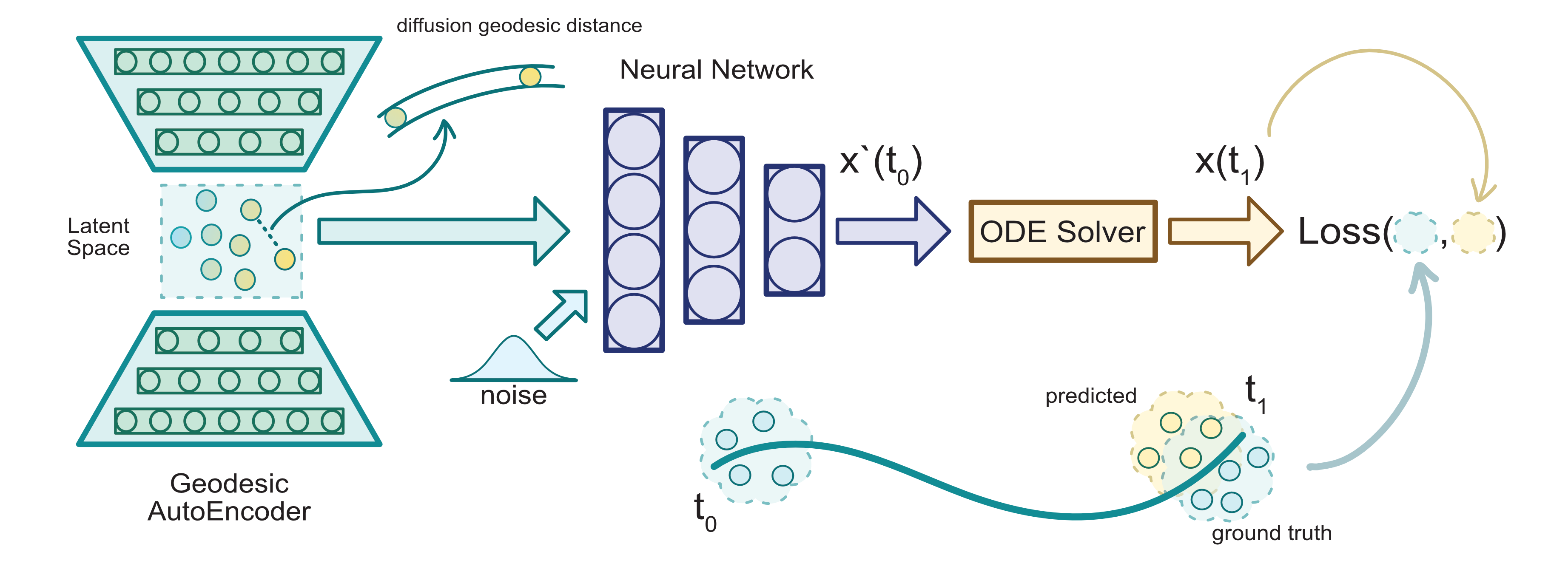
Figure 1: Overview of the MIOFlow pipeline. The Geodesic Autoencoder learns a latent space that preserves the diffusion geodesic distance. A neural network predicts the derivative of the trajectories with respect to time. For an initial sample at $t_{0}$, the ODE Solver produces the trajectories $x(t_{1})$. At a population level, predictions of points at time $t_{1}$ are penalized by the Wasserstein distance during training.

Manifold Geodesics

The dynamic optimal transport formulations (1) and (2) are valid when the ground distance is Euclidean. This is restrictive as we might have observations sampled from a lower dimensional manifold. Thus, using the Euclidean distance in the ambient space ignores the underlying geometry of the data. Static optimal transport with a geodesic distance is known to perform well on geometric domains [40, 45], or when the data lie on a manifold [46]. Here, we extend the use of a ground geodesic distance to the dynamic formulation. To do so, we define a manifold learning step that precedes the trajectory inference. The goal is to learn an embedding $\mathcal{Z}$ such that the Euclidean in $\mathcal{Z}$ is equivalent to the geodesic distance. In that case, dynamic optimal transport in $\mathcal{Z}$ is equivalent to the Wasserstein with a geodesic ground distance. In the following section, we present theoretical results that will justify our approximation of a geodesic distance on a closed Riemannian manifold.

We consider a closed Riemannian manifold $(\mathcal{M},d_{\mathcal{M}})$, where $d_{\mathcal{M}}$ is the geodesic distance representing the shortest path between two points on the manifold. We note $h_{t}$ the heat kernel on $\mathcal{M}$. For a point $x\in\mathcal{M}$, the heat kernel $h_{t}(x,\cdot)$ induces a measure, i.e. how the heat has propagated on the manifold at time $t$ given an arbitrary initial distribution. The diffusion ground distance between $x,y\in\mathcal{M}$ is based on the $L^{1}$ norm between the measures induced by the heat kernel given the initial conditions $\delta_{x}$ and $\delta_{y}$.

Definition 1.

The diffusion ground distance between $x,y\in\mathcal{M}$ is

$$D_{\alpha}(x,y):=\sum_{k\geq 0}2^{-k\alpha}||h_{2^{-k}}(x,\cdot)-h_{2^{-k}}(y,\cdot)||_{1},$$

for $\alpha\in(0,1/2)$, the scale parameter $k\geq 0$, and $h_{t}$ the heat kernel on $\mathcal{M}$.

Next, we state an important result from Leeb and Coifman (Thm. 2 in [25]). This theorem links the diffusion ground distance and the geodesic on a Riemannian manifold.

Theorem 1 ([25] Thm. 2).

Let $(\mathcal{M},d_{\mathcal{M}})$ a closed Riemannian manifold, with geodesic $d_{\mathcal{M}}$, for $\alpha\in(0,1/2)$, the distance $D_{\alpha}$ is equivalent to $d_{\mathcal{M}}^{2\alpha}$.

In practice, we cannot always evaluate the heat kernel for an arbitrary manifold. However, convergence results from Coifman and Lafon [9] provide a natural approximation. Indeed, for $\beta=1$, the diffusion operator $P^{t/\epsilon}_{\epsilon,\beta}$ converges to the heat operator as $\epsilon$ goes to zero (Prop. 3 [9]). For the rest of the paper we assume $\beta=1$, we define $P_{\epsilon}:=P_{\epsilon,1}$ and the matrix $\mathbf{P}_{\epsilon}:=\mathbf{P}_{\epsilon,1}$.

3 Manifold Interpolating Optimal-Transport Flow

To learn individual trajectories from multiple cross-sectional samples of a population, we propose MIOFlow shown in Fig. 1. Our method consists of two steps. We first learn an embedding $\mathcal{Z}$ which preserves the diffusion geodesic distance—which we define using our Geodesic Autoencoder. Then, we learn continuous trajectories based on an optimal transport loss. We model the trajectories with a Neural ODE [7], allowing us to learn non-linear paths and interpolate between timepoints.

3.1 Geodesic Autoencoder Embedding

In light of Thm. 1, we define an approximation of the diffusion ground distance $D_{\alpha}$ (Def. 1) from a collection of samples $\mathsf{X}$ that we call diffusion geodesic distance. We then train an autoencoder regularized to match this distance. Similar ideas are explored in [30, 11] where the latent space of the autoencoder is regularized to match a manifold learning embedding, either PHATE or diffusion map.

Our approximation relies on the diffusion matrix $\mathbf{P}_{\epsilon}$. We first recall its construction. We build a graph with the affinity matrix defined by $(\mathbf{K}_{\epsilon})_{ij}:=k_{\epsilon}(x_{i},x_{j})$, and we consider the density normalized matrix $\mathbf{M}_{\epsilon}:=\mathbf{Q}^{-1}\mathbf{K}_{\epsilon}\mathbf{Q}^{-1}$, where $\mathbf{Q}$ is a diagonal matrix with $\mathbf{Q}_{ii}:=\sum_{j}(\mathbf{K}_{\epsilon})_{ij}$. In practice, we choose $k_{\epsilon}$ to be a Gaussian kernel or the $\alpha$-decay kernel [32]. Lastly, a Markov diffusion operator is defined by $\mathbf{P}_{\epsilon}:=\mathbf{D}^{-1}\mathbf{M}_{\epsilon}$, where $\mathbf{D}_{ii}:=\sum_{j=1}^{n}(\mathbf{M}_{\epsilon})_{ij}$ is a diagonal matrix. The stationary distribution associated to $\mathbf{P}_{\epsilon}$ is $\boldsymbol{\pi}$, where $\boldsymbol{\pi}_{i}=\mathbf{D}_{ii}/\sum_{j}\mathbf{D}_{jj}$, since $\mathbf{P}_{\epsilon}$ is $\boldsymbol{\pi}$-reversible. Finally, we note that the matrix $\mathbf{P}_{\epsilon}$ follows a similar construction as the kernel $p_{\epsilon}$; the integrals are approximated by sums. We refer to [9] for more details about the convergence of the matrix operator $\mathbf{P}_{\epsilon}$ to the operator $P_{\epsilon}$. Until now, we have defined a matrix $\mathbf{P}_{\epsilon}$ that approximates the operator $P_{\epsilon}$, which in turn converges to the heat operator. Now, we define an approximation of the diffusion ground distance, based on the matrix $\mathbf{P}_{\epsilon}$. We use the notation $(\mathbf{P}_{\epsilon})^{t}_{i:}$ to represent the i-th row of $\mathbf{P}^{t}_{\epsilon}$, it represents the transition probabilities of a t-steps random walk started at $x_{i}$.

Definition 2.

We define the diffusion geodesic distance between $x_{i},x_{j}\in\mathsf{X}$ as

$$G_{\alpha}(x_{i},x_{j}):=\sum_{k=0}^{K}2^{-(K-k)\alpha}||(\mathbf{P}_{\epsilon})_{i:}^{2^{k}}-(\mathbf{P}_{\epsilon})_{j:}^{2^{k}}||_{1}+2^{-(K+1)/2}||\boldsymbol{\pi}_{i}-\boldsymbol{\pi}_{j}||_{1}.$$

The diffusion geodesic compares the transitions probabilities of a random walk at various scales given two different initial states $x_{i},x_{j}$. In [46], the authors use the diffusion operator $\mathbf{P}_{\epsilon}$ to define a distance equivalent to the Wasserstein with ground distance $D_{\alpha}$. Their method comes from the static formulation of optimal transport. Here we propose to learn a space $\mathcal{Z}$ that preserves an approximation of the distance $D_{\alpha}$, in order to do dynamic optimal transport in $\mathcal{Z}$.

Training

To use the diffusion geodesic distance, we train a Geodesic Autoencoder, with encoder outputting $\phi:{}^{k}\to\mathcal{Z}$, such that $\|\phi(x_{i})-\phi(x_{j})\|_{2}^{2}\approx G_{\alpha}(x_{i},x_{j})$. We draw a subsample of size $N$, evaluate $G_{\alpha}$ and minimize the Mean Square Error (MSE)

$$L(\phi):=\frac{2}{N}\sum_{i=1}^{N}\sum_{j>i}\left(||\phi(x_{i})-\phi(x_{j})||_{2}-G_{\alpha}(x_{i},x_{j})\right)^{2}.$$

Learning the embedding $\mathcal{Z}$ over using $G_{\alpha}$ as the advantage of being inductive, it is useful since we use it to compute distances between predicted and ground truth observations. Moreover, the encoder can be trained to denoise, hence becoming robust to predicted values that are not close to the manifold. Computing $G_{\alpha}$ on the entire dataset is inefficient due to the powering of the diffusion matrix. We circumvent this difficulty with the encoder, since we train on subsamples. We choose $N$ to have few observations in most regions of the manifold, thus making the computation of $G_{\alpha}$ very efficient, which allows us to consider more scales.

Theorem 2.

Assuming $\mathsf{X}$ is sampled from a closed Riemannian manifold $\mathcal{M}$ with geodesic $d_{\mathcal{M}}$. Then, for all $\alpha\in(0,1/2)$, sufficiently large $K,N$ and small $\epsilon>0$, we have with high probability $G_{\alpha}(x_{i},x_{j})\simeq d_{\mathcal{M}}^{2\alpha}(x_{i},x_{j})$ for all $x_{i},x_{j}\in\mathsf{X}$.

Corollary 1.

If the encoder is such that $L(\phi)=0$, then with high probability $\|\phi(x_{i})-\phi(x_{j})\|_{2}\simeq d_{\mathcal{M}}^{2\alpha}(x_{i},x_{j})$ for all $x_{i},x_{j}\in\mathsf{X}$.

The stochasticity in the two previous results arises from the discrete approximation of the operator $P_{\epsilon}$. The law or large numbers guarantees the convergence. For fix sample size, there exist approximation error bounds with high probability, see for example [8, 39]. In practice, we choose $\alpha$ close to $1/2$ so that the diffusion distance is equivalent to the geodesic on the manifold. From that embedding $\mathcal{Z}$, we can also train a decoder $\phi^{-1}:\mathcal{Z}\to{}^{k}$, with a reconstruction loss $L_{r}:=\sum_{x}\|\phi^{-1}\circ\phi(x)-x\|_{2}$. This is particularly interesting in high dimensions, since we can learn the trajectories in the lower dimensional space $\mathcal{Z}$, then decode them in the ambient space. For example, we use the decoder in Sec. 4 to infer cellular trajectories in the gene space, enabling us to understand how specific genes evolved over time. We describe the training procedure of the GAE in algorithm 2 in the supplementary material.

3.2 Inferring Trajectories

Given $T$ distributions $\{\mu_{i}\}_{i=0}^{T-1}$, we want to model the trajectories respecting the conditions $X_{i}\sim\mu_{i}$ for fix timepoints $i\in\{0,\dotsc,T-1\}$. Formally, we want to learn a parametrized function $f_{\theta}(x,t)$ such that

$$X_{t}=X_{0}+\int_{0}^{t}f_{\theta}(X_{u},u)du,\;\text{with }X_{0}\sim\mu_{0},\dotsc,X_{T-1}\sim\mu_{T-1}.$$ (4)

We adapt the main theorem from [44], to consider the path space, and other types of dissimilarities between distributions.

Theorem 3.

We consider a time-varying vector field $f(x,t)$ defining the trajectories $dX_{t}=f(X_{t},t)dt$ with density $\rho_{t}$, and a dissimilarity between distributions such that $D(\mu,\nu)=0$ iff $\mu=\nu$. Given these assumptions, there exist a sufficiently large $\lambda>0$ such that

$$W_{2}(\mu,\nu)^{2}=\inf_{X_{t}}E\bigg{[}\int_{0}^{1}\|f(X_{t},t)\|_{2}^{2}dt\bigg{]}+\lambda D(\rho_{1},\nu)\,\text{ s.t. }\,X_{0}\sim\mu.$$ (5)

Moreover, if $X_{t}$ is defined on the embedded space $\mathcal{Z}$, then $W_{2}$ is equivalent to the Wasserstein with geodesic distance $W_{2}(\mu,\nu)\simeq W_{d_{\mathcal{M}}^{2\alpha}}(\mu,\nu)$.

This theorem enables us to add the second marginal constraint in the optimization problem. In practice, it justifies the method of matching the marginals and adding a regularization on the vector field $f(x,t)$, that way the optimal $(\rho_{t},f)$ corresponds to the one from the $W_{2}$. If in addition we model the trajectories in the embed space $\mathcal{Z}$, then the transport is equivalent to the one on the manifold.

Training

We observe discrete distributions $\boldsymbol{\mu}_{i}:=(1/n_{i})\sum_{i}\delta_{x_{i}}$ for $x_{i}\in\mathsf{X}_{i}$, and we approximate (4) with a Neural ODE [7], where $f_{\theta}$ is modeled by a neural network with parameters $\theta$. Denote by $\psi_{\theta}:{}^{k}\times\mathcal{T}\to{}^{d|\mathcal{T}|}$ the function that represents the Neural ODE, where $\mathcal{T}$ is a set of time indices. We define the predicted sets $\widehat{\mathsf{X}}_{1},\dotsc,\widehat{\mathsf{X}}_{T-1}=\psi_{\theta}(\mathsf{X}_{0},\{1,\dotsc,T-1\})$; given an initial set $\mathsf{X}_{0}$ it returns the approximation of $\eqref{eq: traj}$ for all $t\in\mathcal{T}$. The resulting discrete distributions are $\hat{\boldsymbol{\mu}}_{i}:=(1/n_{i})\sum_{j}\delta_{x_{j}}$ for $x_{j}\in\widehat{\mathsf{X}}_{i}$. To match the marginals, we used two approaches of training; local or global. For the local method, we only predict the next sample, hence given $\mathsf{X}_{t}$ as initial condition, we predict $\widehat{\mathsf{X}}_{t+1}=\psi_{\theta}(\mathsf{X}_{t},t+1)$. Whereas for the global, we use the entire trajectories given the initial condition $\mathsf{X}_{0}$. For both cases, we formulate a loss $L_{m}$ on the marginals, representing the second term in (5). To take into account the first term in (5), we add the loss $L_{e}$, where the integral can be approximate with the forward pass of the ODE solver, and $\lambda_{e}\geq 0$ is a hyperparameter.

$$L_{m}:=\sum_{i=1}^{T-1}W_{2}(\hat{\boldsymbol{\mu}}_{i},\boldsymbol{\mu}_{i})\qquad L_{e}:=\lambda_{e}\sum_{i=0}^{T-2}\int_{i}^{i+1}\|f_{\theta}(x_{t},t)\|_{2}^{2}dt$$ (6)

In practice, to compute the Wasserstein between discrete distributions, we use the implementation from the library Python Optimal Transport [14]. This is in contrasts with the maximum-likelihood approach in CNF methods which requires evaluation of the instantaneous change of variables at every integration timestep at $O(k^{2})$ additional cost per function evaluation [7].

We add a final density loss $L_{d}$ inspired by [44] to encourage the trajectories to stay on the manifold. Intuitively, for a predicted point $x\in\widehat{\mathsf{X}}_{t}$, we minimize the distance to its k-nearest neighbors in $\mathsf{X}_{t}$ given a lower bound $h>0$

$$L_{d}:=\lambda_{d}\sum_{t=1}^{T-1}\sum_{x\in\widehat{\mathsf{X}}_{t}}\ell_{d}(x,t),\,\text{ where }\,\ell_{d}(x,t):=\sum_{i=1}^{k}\max(0,\text{min-k}(\{\|x-y\|:y\in\mathsf{X}_{t}\})-h).$$

We describe the overall training procedure of MIOFlow in algorithm 1.

Modeling Diffusion

We add a diffusion term in the trajectories, resulting in the SDE $dX_{t}=f(X_{t},t)dt+\sqrt{\sigma_{t}}dB_{t}$ In practice, we learn $T$ parameters $\{\sigma_{t}\}_{t=0}^{T-1}$ It has the advantage of mapping the same cell to different trajectories stochastically as in many naturalistic systems. Early in the training process, we notice that it promotes bifurcation, as it helps to spread the initial $\mathsf{X}_{0}$. As training continues, we empirically observed that $\sigma\to 0$. Hence, as shown in [28], converging to the $W_{2}$ formulation. For small $\sigma_{t}$, we train with a regular ODE solver, essentially corresponding to the Euler–Maruyama method. To model complex diffusion, one would need an SDE solver, thus drastically increasing the computational cost.

Algorithm 1 MIOFlow

Input: Datasets $\mathsf{X}_{0},\dotsc,\mathsf{X}_{T-1}$, graph kernel $\mathbf{K}_{\epsilon}$, maximum scale $K$, noise scale $\xi$, batch size $N$, maximum iteration $n_{max}$, initialized encoder $\phi$ and decoder $\phi^{-1}$, maximum local iteration $n_{local}$, maximum global iteration $n_{global}$, initialized neural ODE $\psi_{\theta}$.

Output: Trained neural ODE $\psi_{\theta}$.

GAE: $\phi,\phi^{-1}\leftarrow\text{GAE}(\mathsf{X},\mathbf{K}_{\epsilon},K,\xi,N,n_{max},\phi,\phi^{-1})$ $\triangleright$ See algorithm 2 in SM

if use GAE then $\mathsf{X}_{0},\dotsc,\mathsf{X}_{T-1}\leftarrow\phi(\mathsf{X}_{0}),\dotsc,\phi(\mathsf{X}_{T-1})$

end if

for i=1 to $n_{local}$ do $\triangleright$ Local training

     for t=0 to $T-2$ do

         $\widehat{\mathsf{X}}_{t+1}\leftarrow\psi_{\theta}(\mathsf{X}_{t},t+1)$

     end for

     $L\leftarrow L_{m}+L_{e}+L_{d}$

     update $\psi_{\theta}$ with gradient descent w.r.t. the loss $L$

end for

for i=1 to $n_{global}$ do $\triangleright$ Global training

     $\widehat{\mathsf{X}}_{1},\dotsc,\widehat{\mathsf{X}}_{T-1}\leftarrow\psi_{\theta}(\mathsf{X}_{0},\{1,\dotsc,T-1\})$

     $L\leftarrow L_{m}+L_{e}+L_{d}$

     update $\psi_{\theta}$ with gradient descent w.r.t. the loss $L$

end for

4 Results

Here, we validate our method empirically on both synthetic test cases and single-cell RNA sequencing datasets chosen to test the capability of MIOFlow to follow divergent trajectories from population snapshot data. Using these test cases we assess whether MIOFlow-derived trajectories qualitatively follow the data manifold efficiently, we also quantitatively assess their accuracy using the Wasserstein $W_{1}$, and Maximum Mean Discrepancy (MMD) [18] on held-out timepoints. The MMD is evaluated with the Gaussian (G) kernel and the mean (M). We compare our results to those other methods that preform population flows including TrajectoryNet [44] which is based on a CNF that is regularized to achieve efficient paths, and Diffusion Schrödinger’s Bridge (DSB) [10] which is an optimal transport framework for generative modeling. The baseline measure in the quantitative results corresponds to the average distance between the previous and next timepoints for a given time $t$. Additional experiments, such as ablation studies, and details are provided in the supplementary material.

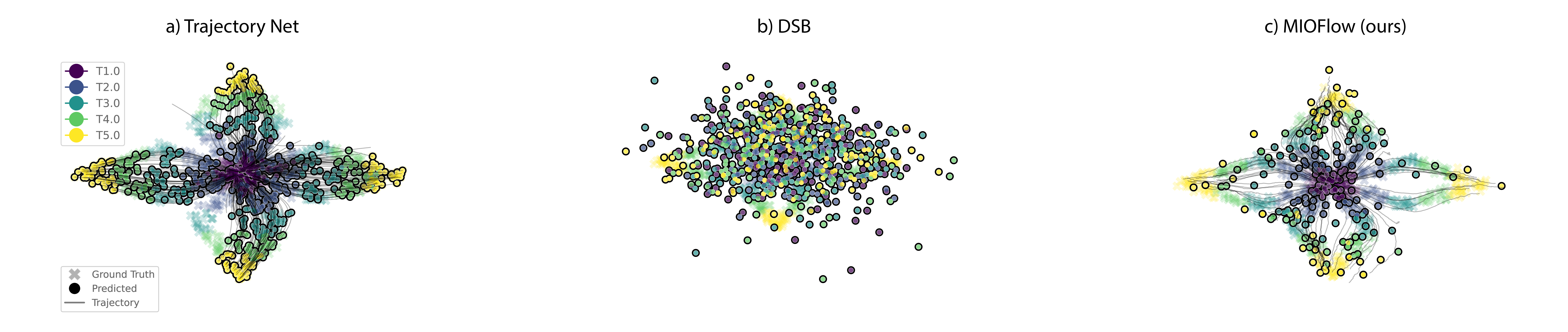
Figure 2: Comparisons between predicted flows of (a) TrajectoryNet, (b) DSB, and (c) MIOFlow on a toy Petal dataset. MIOFlow trajectories both match the data and transition along the data manifold whereas TrajectoryNet takes shortcut paths between the the curved paths and Schroedinger’s bridge does not follow the data. Time is indicated by color. Ground truth points are designated by translucent “X”s in the background, whereas predicted points are opaque circles, whilst trajectories are solid lines.

4.1 Artificial Data

Petal

The petal dataset is a simple yet challenging, as it mimics natural dynamics arising in cellular differentiation, including bifurcations and merges. The dynamics start in the center (purple) and evolves through the end of the leaf (yellow). In Fig. 2, we present the trajectories on the petal dataset for TrajectoryNet, DSB, and MIOFlow. Only our method is able to learn the dynamic, and keeping trajectories on the manifold. We then hold-out timepoint $2$ corresponding to the initial bifurcation, and, in Tab. 1, we compare the interpolation between the three methods. MIOFlow results in a more accurate entropic interpolation for both $W_{1}$ and MMD(G), while requiring much less computational time. In the supplementary material, we present additional results for DSB on the petal dataset.

Dyngen

We use Dyngen [6] to simulate a scRNA-seq dataset from a dynamical cellular process. We first embed the observations in five dimensions using the non-linear dimensionality reduction method PHATE [32]. We discretize the space in five bins, each representing a differentiation stage. This dataset includes one bifurcation. However, it proves more challenging than the petal dataset. The number of samples per bins is not equal, which tends to give more influence to the lower branch. Moreover, the bifurcation is asymmetric; the curve in the lower branch is less pronounce than the upper one, making it harder to learn a continuous bifurcation. In Fig. 3, we show the trajectories for TrajectoryNet, DSB, and our method. MIOFlow is more accurate as it learns continuous bifurcating trajectories along the two main branches. In Tab. 1, we hold-out timepoint 2, and show the interpolation results against the ground truth. MIOFlow is more accurate for all metrics, while requiring much less computational time. We see that in timepoint 1, TrajectoryNet deviates far from the trajectories particularly at the branching point where it struggles with induced heterogeneity (see Fig. 3). We have further quantifications reflecting this in the supplementary material.

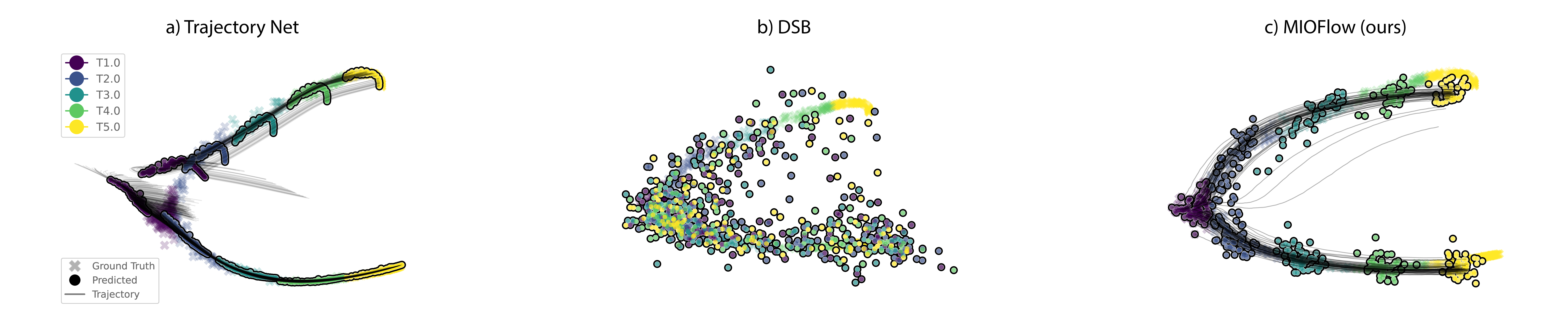
Figure 3: Comparisons between predicted flows of (a) TrajectoryNet, (b) DSB, and (c) MIOFlow on Dyngen [6] simulated dataset. MIOFlow trajectories both match the data and transition along the data manifold throughout the timepoints. Time is indicated by color. Ground truth points are designated by translucent “X”s in the background, whereas predicted points are opaque circles, whilst trajectories are solid lines.

Table 1: Leave-one-out $W_{1}$ and MMD with (G)aussian or (M)ean kernel between the predicted and ground truth points as well as training time in (m)inutes and (s)econds on the Petal and Dyngen datasets of TrajectoryNet, DSB, and MIOFlow. Lower is better.

	Petal				Dyngen
	$W_{1}$	MMD(G)	MMD(M)	Runtime	$W_{1}$	MMD(G)	MMD(M)	Runtime
MIOFlow (ours)	0.090	0.029	0.005	284.60 (s)	0.783	0.199	0.509	95.63 (s)
TrajectoryNet	0.181	0.136	0.002	64 (m)	1.499	0.303	1.806	62 (m)
DSB	0.199	0.157	0.008	86 (m)	2.051	0.932	2.367	81 (m)
Baseline	0.221	0.196	$<$0.001	N/A	1.388	1.008	0.926	N/A

4.2 Single-Cell Data

Embryoid Body

Here we evaluate our method on scRNA-seq data from the dynamic time course of human embryoid body (EB) differentiation over a period of 27 days, measured in 3 timepoints between days 0-3, 6-9, 12-15, 18-21, and 24-27. We reduce the dimensionality of this dataset to 200 dimensions using PCA. See the supplementary material for further details on the preprocessing steps and the parameters.

By combining PCA and the autoencoder with diffusion geodesic distance described in section 3.1, we can decode the trajectories back into the gene space (17846 dimensions), thus describing the evolution of the gene expression of a cell. In Fig. 5 we plot the trajectories, at a gene level of 20 neuronal cells against 20 random one. We generally observe distinct differences between TrajectoryNet and MIOFlow. TrajectoryNet (which is shown in the bottom) shows a tendency to have early divergence in trends artificially showing higher heterogeneity in gene trends then exist in neuronal specification processes. Examples include HAND2, which has a non-monotonic trend, first increasing in expression during development from embryonic stem cells to neural early progenitors and then decreasing as the lineages mature [26]. MIOFlow clearly shows this trend whereas TrajectoryNet trends are more chaotic. Another example is ONECUT2 which is consistently known to be higher in cells that diverge towards the neuronal lineage [48]. Other examples are discussed in the supplementary material.

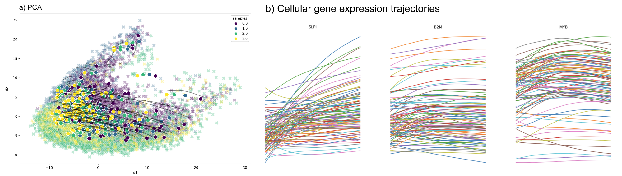
Figure 4: MIOFlow on the AML dataset. a) PCA Embedding comparing ground truth to MIOFlow predicted points and trajectories. b) Cellular gene expression trajectories for SLPI, B2M, and MYB for MIOFlow.

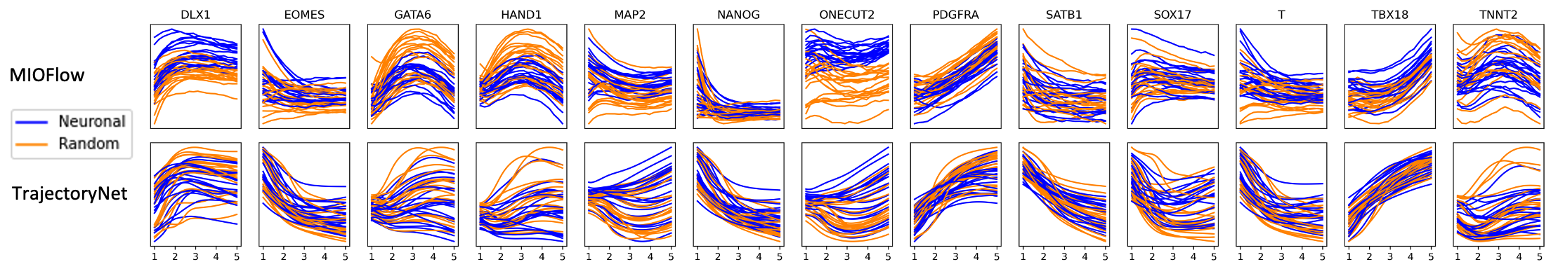
Figure 5: Neuronal gene trajectories vs. random trajectories for MIOFlow (top) vs. TrajectoryNet [46] (bottom). TrajectoryNet consistently shows a tendency for early divergence in trajectories, examples include ONECUT2 which is biologically known to be higher expressed [32] and HAND2 which is known to peak in neural early progenitors (NEPs).

In Tab. 2, we compare the prediction accuracy of MIOFlow whether we use the GAE embedding or no embedding. For the GAE, we show results for two kernels; the Gaussian kernel (scale $0.5$), and the $\alpha$-decay kernel [32] (based on a 30 nearest neighbors graph). For almost all metrics, the prediction accuracy is greater with the GAE. We present additional results for the choice of kernel in the supplementary material.

Table 2: Leave-one-out $(t)$ $W_{1}$ and MMD with (G)aussian and (M)ean kernel between the predicted and ground truth point on the EB datasets for MIOFlow with the Gaussian, $\alpha$-decay kernel, or without GAE. Lower is better.

	$t=2$			$t=3$
	$W_{1}$	MMD(G)	MMD(M)	$W_{1}$	MMD(G)	MMD(M)
GAE Gaussian	26.318	0.059	101.969	32.963	0.138	223.679
GAE $\alpha$-decay	25.744	0.061	99.747	32.227	0.135	213.465
No GAE	29.243	0.063	126.608	35.709	0.119	246.609
Baseline	33.415	0.103	227.279	35.319	0.095	213.492

AML Cancer Data with Treatment-based Progression

We also assessed whether MIOFlow can give insights on treatment resistant cancer cell populations, rather than differentiation. For this purpose, we used data from Fennell et al. [12] in which AF9 mutant cancer cells implanted into the bone marrow of mice as a model of Acute Myeloid Leukemia (AML). The mice are then treated for 7 days with intensive chemotherapy with single cell measurements taken at day 2, day 5, and day 7. Here we show MIOFlow on this dataset along with signatures of leukemic stem cells (LSCs) which are hypothesized to be dominant in chemotherapy resistant cells. We see heterogeneity in the trajectories, the majority of cells surviving to the last timepoint showing an increase in the markers SLPI, MYB, and B2M—all members of the LSC pathway [12]. This indicates that not all cells start with this signature but are made to transition to this signature to resist the effects of chemotherapy.

5 Related Work

The task of recovering dynamics from multiple snapshots has gained a lot of attention, especially in biology with scRNA-seq data. Static methods such as pseudotime assign an abstract measure of time for all cells depending on an initial state [19, 47]. In can be combined to infer the cell lineage, i.e. the principal curves or trajectories [43]. When estimates of cell growth rates are available, Zhang et al. [52] proposed a method based on optimal transport. Another line of research is on the direct rate of differentiation of cell or RNA velocity [23, 4]. This method does not provide trajectories, but it can be combined to define a transition matrix to infer trajectories [53]. Saelens et al. [37] provide a rigorous comparison of 45 static methods.

Similar methods used the dynamic formulation of optimal transport [5, 13, 20, 35, 36, 38, 44] to infer trajectories. The dynamics are either modeled with a recurrent neural network [20], a generative adversarial networks [35], flows defined by the gradient of an input convex neural network [5], or a CNF [44]. Here, we circumvent the need for a CNF by modeling the trajectories directly on the support of the distributions, hence maintaining the computational cost low even in high dimension. Some generative methods that interpolate between a prior to a target can also be used to recover trajectories. Other methods use the Schrödinger bridge (SB)  [10, 22, 49, 51] problem to define trajectories between distributions. For example [10], solve the SB between two distributions using a series of Sinkhorn iterations. However, it does not explicitly learn dynamics, making their interpolations inaccurate.

6 Conclusion

We proposed MIOFlow a computationally efficient method to recover trajectories from multiple cross-sectional samples of a time-evolving population. Our method includes a novel manifold learning framework, where we learn an embedding preserving the geodesic distance. We show theoretically how MIOFlow is related to dynamical optimal transport on an underlying manifold, and it’s capacity to model stochastic trajectories. On artificial datasets, MIOFlow produced continuous trajectories more in line with the manifold compared to DSB and TrajectoryNet. On scRNA-seq data, we leveraged an autoencoder with the geodesic embedding to learn the trajectories in a lower dimensional space while preserving meaningful distances which can then be decoded in gene space. This way we could visualize the evolution of the gene expression of a cell.

7 Limitations and Broader Impact

Our method does have some limitations. Similarly to other works based on continuous time networks, our work makes use of generic ODE solvers and adjoint dynamics which can fail under stiff dynamics. Like other methods that learn dynamics it is possible that the learned dynamics may become stiff through training leading to decreased model accuracy. In addition, our work is sensitive to the time-bins, and it worked best for relatively uniform sampling. This second issue could potentially be alleviated by using unbalanced optimal transport, which allows transporting distributions with unequal masses. Our work can help understand dynamical systems, and in particular cellular differentiation, and thus to the best of our knowledge presents no potential negative societal impacts.

1. For all authors…

   1. Do the main claims made in the abstract and introduction accurately reflect the paper’s contributions and scope? [Yes]

   2. Did you describe the limitations of your work? [Yes] In the limitations and broader impact section.

   3. Did you discuss any potential negative societal impacts of your work?

      [Yes] In the limitations and broader impact section. We do not foresee any immediate negative societal impacts of this work.

   4. Have you read the ethics review guidelines and ensured that your paper conforms to them? [Yes]

2. If you are including theoretical results…

   1. Did you state the full set of assumptions of all theoretical results?

      [Yes] We stated all assumptions in the main body of the text and provide additional details in the supplementary materials.

   2. Did you include complete proofs of all theoretical results?

      [Yes] Complete proofs are available in the supplement.

3. If you ran experiments…

   1. Did you include the code, data, and instructions needed to reproduce the main experimental results (either in the supplemental material or as a URL)?

      [Yes] Code and links to publicly available data are provided in the supplemental material.

   2. Did you specify all the training details (e.g., data splits, hyperparameters, how they were chosen)?

      [Yes] All training details are provided in the supplement.

   3. Did you report error bars (e.g., with respect to the random seed after running experiments multiple times)? [Yes]

   4. Did you include the total amount of compute and the type of resources used (e.g., type of GPUs, internal cluster, or cloud provider)?

      [Yes] Compute resources are discussed in the supplement.

4. If you are using existing assets (e.g., code, data, models) or curating/releasing new assets…

   1. If your work uses existing assets, did you cite the creators? [Yes]

   2. Did you mention the license of the assets? [Yes] See supplement

   3. Did you include any new assets either in the supplemental material or as a URL? [Yes]

   4. Did you discuss whether and how consent was obtained from people whose data you’re using/curating? [N/A]

   5. Did you discuss whether the data you are using/curating contains personally identifiable information or offensive content?

      [Yes] Our data does not contain any personally identifiable information or offensive content. The Embryoid body data is a cell culture, and the AML Cancer dataset is patient derived but contains no identifiable information.

5. If you used crowdsourcing or conducted research with human subjects…

   1. Did you include the full text of instructions given to participants and screenshots, if applicable? [N/A]

   2. Did you describe any potential participant risks, with links to Institutional Review Board (IRB) approvals, if applicable? [N/A]

   3. Did you include the estimated hourly wage paid to participants and the total amount spent on participant compensation? [N/A]

Appendix A Theory and Algorithm

A.1 Geodesic Autoencoder Algorithm

Using the definitions from Sec. 3, we present the algorithm to train the geodesic autoencoder.

Algorithm 2 Geodesic Autoencoder (GAE)

Input: Dataset $\mathsf{X}$ of size $n$, graph kernel $\mathbf{K}_{\epsilon}$, maximum scale $K$, noise scale $\xi$, batch size $N$, maximum iteration $n_{max}$, initialized encoder $\phi$ and decoder $\phi^{-1}$.

Output: Trained encoder $\phi$ and decoder $\phi^{-1}$.

for i=1 to $n_{max}$ do

     Sample batch $\{x_{1},\dotsc,x_{N}\}\subseteq\mathsf{X}$ of size $N$

     $\mathbf{Q}\leftarrow\text{diag}(\sum_{j}(\mathbf{K}_{\epsilon})_{ij})$

     $\mathbf{M}_{\epsilon}\leftarrow\mathbf{Q}^{-1}\mathbf{K}_{\epsilon}\mathbf{Q}^{-1}$

     $\mathbf{D}\leftarrow\text{diag}(\sum_{j}(\mathbf{M}_{\epsilon})_{ij})$

     $\mathbf{P}_{\epsilon}\leftarrow\mathbf{D}^{-1}\mathbf{M}_{\epsilon}$ $\triangleright$ $N\times N$ diffusion matrix

     $G_{\alpha}\leftarrow 2^{-K\alpha}\,\text{pairwise\_distances}((\mathbf{P}_{\epsilon})_{1:},\dotsc,(\mathbf{P}_{\epsilon})_{N:})$

     for k=1 to K do

         $G_{\alpha}\leftarrow G_{\alpha}+2^{-(K-k)\alpha}\,\text{pairwise\_distance}((\mathbf{P}^{2^{k}}_{\epsilon})_{1:},\dotsc,(\mathbf{P}^{2^{k}}_{\epsilon})_{N:})$

     end for

     $\tilde{x}_{1},\dotsc,\tilde{x}_{N}\leftarrow x_{1}+\xi z_{1},\dots,x_{N}+\xi z_{N}$, where $\{z_{1},\dotsc,z_{N}\}\sim\mathcal{N}(0,1)$

     $L\leftarrow$ MSE$\big{(}\text{pairwise\_distances}(\phi(\tilde{x}_{1}),\dotsc,\phi(\tilde{x}_{N})),G_{\alpha}\big{)}$

     $L_{r}\leftarrow\sum_{i}\|\phi^{-1}\circ\phi(\tilde{x}_{i})-x\|_{2}$

     Update $\phi,\phi^{-1}$ with gradient descent w.r.t. $L(\phi),L_{r}(\phi,\phi^{-1})$

end for

A.2 Proof of Thm.2

Theorem 2.

Assuming $\mathsf{X}$ is sampled from a closed Riemannian manifold $\mathcal{M}$ with geodesic $d_{\mathcal{M}}$, then for a sufficiently large $K,N$ and small $\epsilon>0$, we have $G_{\alpha}(x_{i},x_{j})\simeq d_{\mathcal{M}}^{2\alpha}(x_{i},x_{j})$, for all $\alpha\in(0,1/2)$.

Proof.

We adapt the convergence proof from [46], it can be summarized in two parts. First, the equivalence of the distances defined by $P_{\epsilon}^{t/\epsilon}$ and the heat operator $H_{t}$. This relies on the convergence results $P_{\epsilon}^{t/\epsilon}\to H_{t}$ as $\epsilon\to 0$ from Coifman and Lafon [9]. Second, the approximation of the operator $P_{\epsilon}$ based on a finite set of points. Throughout the proof we use the same notation $\delta_{x}$ for the delta Dirac function, and $\delta_{x_{i}}$ for a row vector with $i$-th element $1$, and $0$ otherwise.

For a family of operator $(A_{t})_{t\in\real}$ we define

$$D_{\alpha,A}(x,y):=\sum_{k\geq 0}2^{-k\alpha}||A_{2^{-k}}(x,\cdot)-A_{2^{-k}}(y,\cdot)||_{1},$$

and equivalently $D_{\alpha,A}(x,y)=\sum 2^{-k\alpha}||A_{2^{-k}}(\delta_{x}-\delta_{y})||_{1}$, where $A\delta_{x}:=\int A(u,\cdot)\delta_{x}(u)du$. This definition is the same as Def. 1, but for an arbitrary operator. Our final goal is to show that $G_{\alpha}(x_{i},x_{j})\simeq D_{\alpha,H_{t}}(x_{i},x_{j})$, and then conclude with Thm. 1 which gives the equivalence $D_{\alpha,H_{t}}(x_{i},x_{j})\simeq d^{2\alpha}_{\mathcal{M}}(x_{i},x_{j})$.

We first want to show that, for a sufficiently small $\epsilon>0$, we have $D_{\alpha,P_{\epsilon}^{t/\epsilon}}(x,y)\simeq D_{\alpha,H_{t}}$, where $P$ is the anisotropic operator defined in Sec. 2. From Coifman and Lafon [9], we have $\|P_{\epsilon}^{t/\epsilon}-H_{t}\|_{L^{2}(\mathcal{M})}\to 0$ as $\epsilon\to 0$, and also $\|P_{\epsilon}^{t/\epsilon}-H_{t}\|_{L^{1}(\mathcal{M})}\to 0$.

Now let $\Gamma_{t}:=P_{\epsilon}^{t/\epsilon}-H_{t}$, and for $\gamma>0$ choose $\epsilon>0$ such that $\|\Gamma_{t}(\delta_{x}-\delta_{y})\|_{1}<\gamma\|\delta_{x}-\delta_{y}\|_{1}=2\gamma$ for $x\neq y$, we have

$$D_{\alpha,\Gamma_{t}}(x,y)=\sum_{k\geq 0}2^{-k\alpha}||\Gamma_{2^{-k}}(\delta_{x}-\delta_{y})||_{1}\leq 2\gamma\sum_{k\geq 0}2^{-k\alpha}=\frac{2\gamma}{1-2^{-\alpha}}.$$

Thus, for all $t>0$, and all $\gamma>0$ there exists $\epsilon>0$ such that $D_{\alpha,\Gamma_{t}}(x,y)<\gamma$. From the reverse triangle inequality, we have

$$|D_{\alpha,P_{\epsilon}^{t/\epsilon}}(x,y)-D_{\alpha,H_{t}}|\leq D_{\alpha,\Gamma_{t}}(x,y),$$

using $D_{\alpha,\Gamma_{t}}(x,y)<\gamma$, we obtain

$$D_{\alpha,H_{t}}(x,y)-\gamma\leq D_{\alpha,P_{\epsilon}^{t/\epsilon}}(x,y)\leq D_{\alpha,H_{t}}(x,y)+\gamma.$$

According to wang1997sharp we can lower bound the heat kernel, and thus the distance $D_{\alpha,H_{t}}(x,y)>C$ for some $C>0$. For $\gamma<C/2$, and a sufficiently small $\epsilon>0$, we have

$$(1/2)D_{\alpha,H_{t}}(x,y)\leq D_{\alpha,P_{\epsilon}^{t/\epsilon}}(x,y)\leq(3/2)D_{\alpha,H_{t}}(x,y).$$

This proves our first claim, that $D_{\alpha,P_{\epsilon}^{t/\epsilon}}(x,y)\simeq D_{\alpha,H_{t}}$ for small $\epsilon>0$.

Next, we consider the approximation of the operator $P_{\epsilon}^{t/\epsilon}$ with a finite set of points. Now we define

$$G_{K,\epsilon,\alpha}(x_{i},x_{j}):=\sum_{k=0}^{K}2^{-k\alpha}||(\delta_{x_{i}}-\delta_{x_{j}})\mathbf{P}_{\epsilon}^{2^{-k}/\epsilon}||_{1},$$

if $\epsilon=2^{-K}$, then the first term of $G_{\alpha}(x_{i},x_{j})$ is equal to $G_{K,\epsilon,\alpha}(x_{i},x_{j})$. Since we will let $K\to\infty$, we ignore the second term in $G_{\alpha}(x_{i},x_{j})$, as it converges to zero. Similar to Coifman and Lafon [9] (Sec. 5), we have $\mathbf{P}\to P$ as $n\to\infty$, using Monte-Carlo integration (approximation of integral with summation by the law of large numbers). By the strong law of large numbers, the convergence is with probability one. For a finite number of samples, we have a high probability bound on the convergence, see for example [8, 39]. Now we let $N:=\min(K,n)$, and therefore

$$\lim_{N\to\infty}G_{K,\epsilon,\alpha}(x_{i},x_{j})=D_{\alpha,P_{\epsilon}^{t/\epsilon}}(x_{i},x_{j}).$$

Hence, if we take $\epsilon:=2^{-K}$, we have for sufficiently large $n$ and $K$ (implying small $\epsilon>0$), $G_{\alpha}(x_{i},x_{j})\simeq D_{\alpha,H_{t}}\simeq d^{2\alpha}_{\mathcal{M}}(x_{i},x_{j})$ from Thm. 1. ∎

A.3 Proof of Thm.3

Theorem 3.

We consider a time-varying vector field $f(x,t)$ defining the trajectories $dX_{t}=f(X_{t},t)dt$ with density $\rho_{t}$, and a dissimilarity between distributions such that $D(\mu,\nu)=0$ iff $\mu=\nu$. Given these assumptions, there exist a sufficiently large $\lambda>0$ such that

$$W_{2}(\mu,\nu)^{2}=\inf_{X_{t}}E\bigg{[}\int_{0}^{1}\|f(X_{t},t)\|_{2}^{2}dt\bigg{]}+\lambda D(\rho_{1},\nu)\,\text{ s.t. }\,X_{0}\sim\mu.$$

Moreover, if $X_{t}$ defined on the embedded space $\mathcal{Z}$, then $W_{2}$ is equivalent to the Wasserstein with geodesic distance $W_{2}(\mu,\nu)\simeq W_{d_{\mathcal{M}}^{2\alpha}}(\mu,\nu)$.

Proof.

We recall that

$$W_{2}(\mu,\nu)^{2}=\inf_{X_{t}}\mathbb{E}\bigg{[}\int_{0}^{1}\|f(X_{t},t)\|_{2}^{2}dt\bigg{]}\,\text{ s.t. }dX_{t}=f(X_{t},t)dt,\,X_{0}\sim\mu,\,X_{1}\sim\nu,$$

is equivalent to

$$W_{2}(\mu,\nu)^{2}=\inf_{(\rho_{t},v)}\int_{0}^{1}\int_{{}^{k}}\|v(x,t)\|^{2}\rho_{t}(dx)dt,$$

with the three constraints

$$\textit{a)}\,\partial_{t}\rho_{t}+\nabla\cdot(\rho_{t}v)=0\quad\textit{b)}\,\rho_{0}=\mu,\quad\textit{c)}\,\rho_{1}=\nu.$$

Tong et al. [44] (Thm. 4.1), showed that, for large $\lambda>0$ and $\rho_{t}$ satisfying a), this minimization problem is equivalent to

$$W_{2}(\mu,\nu)^{2}=\inf_{(\rho_{t},v)}\int_{0}^{1}\int_{{}^{k}}\|v(x,t)\|^{2}\rho_{t}(dx)dt+\lambda KL(\rho_{1}\,||\nu),$$

where KL is the Kullback–Leibler divergence, we note that their proof is valid for any dissimilarity $D(\rho_{1}\,||\nu)$ respecting the identity of indiscernibles. Using the path formulation, by writing the integral as an expectation and taking the infimum over all absolutely continuous path, we have

$$W_{2}(\mu,\nu)^{2}=\inf_{X_{t}}E\bigg{[}\int_{0}^{1}\|f(X_{t},t)\|_{2}^{2}dt\bigg{]}+\lambda D(\rho_{1},\nu)\,\text{ s.t. }\,dX_{t}=f(X_{t},t)dt,\,X_{0}\sim\mu.$$

Assuming the encoder $\phi$ achieves a loss of zero, then from Corr. 1 for $\alpha\in(0,1/2)$, we have $\|\phi(x_{i})-\phi(x_{j})\|_{2}\simeq d^{2\alpha}_{\mathcal{M}}(x_{i},x_{j})$ for all $x_{i},x_{j}\in\mathsf{X}\subseteq\mathcal{M}$, and sufficiently large $n$ and $K$. That is, there exist $c,C>0$ such that $c\,d_{\mathcal{M}}(x_{i},x_{j})\leq\|\phi(x_{i})-\phi(x_{j})\|_{2}\leq Cd_{\mathcal{M}}(x_{i},x_{j})$ for all $x_{i},x_{j}\in\mathsf{X}$. Then, for all $\pi\in\Pi(\mu,\nu)$, we have

$$c^{p}\int_{\mathsf{X}\times\mathsf{X}}d^{2\alpha}_{\mathcal{M}}(x,y)^{p}\pi(dx,dy)\leq\int_{\mathsf{X}\times\mathsf{X}}\|\phi(x)-\phi(y)\|_{2}^{p}\pi(dx,dy)\leq C^{p}\int_{\mathsf{X}\times\mathsf{X}}d^{2\alpha}_{\mathcal{M}}(x,y)^{p}\pi(dx,dy),$$

and taking the infimum with respect to $\pi\in\Pi(\mu,\nu)$ yields the desired result $W_{2}(\mu,\nu)\simeq W_{d_{\mathcal{M}}^{2\alpha}}(\mu,\nu)$. ∎

A.4 Schrödinger bridge

Let $\mathcal{D(\mu,\nu)}$ the space of probability distributions on $\mathcal{C}:=C([0,1],{}^{k})$, with initial and final distribution $\mu$ and $\nu$, and $N$ the Wiener measure on $\mathcal{C}$, then the Schrödinger bridge (SB) problem is to find the time-evolving distribution $\rho_{t}$ such that

$$\min\mathrm{KL}(\rho_{t}\,||N)\text{ subject to }\rho_{t}\in\mathcal{D}(\mu,\nu),$$

where $\mathrm{KL}$ is the Kullback–Leibler divergence. It also admits a static formulation, i.e. minimizing with respect to $\pi\in\Pi(\mu,\nu)$. Using the measure $N_{x}^{y}$ over a Brownian bridge with initial and final condition $x$ and $y$, and $\rho_{x}^{y}$ defined similarly for $\rho\in\mathcal{D(\mu,\nu)}$, we can write $KL(\rho_{t}\,||N)=KL(\pi\,||\pi^{N})+KL(\rho_{x}^{y}\,||N_{x}^{y})$, where $\pi^{N}$ is the joint distribution between the initial and final states under the Wiener measure $N$. By choosing $\rho_{x}^{y}=N_{x}^{y}$, the static formulation of the Schrödinger bridge is

$$\min\mathrm{KL}(\pi\,||\pi^{N})\text{ subject to }\pi\in\Pi(\mu,\nu).$$

When the Wiener measure has variance $\sigma^{2}$, the static Schrödinger bridge is equivalent to minimizing

$$\inf_{\pi\in\Pi(\mu,\nu)}\int_{{}^{k}\times{}^{k}}(1/2)||x-y||_{2}^{2}\pi(dx,dy)+\sigma^{2}H(\pi),$$

where $H$ is the entropy (see [33] and references therein). That is an optimal transport problem with entropic regularization, the same formulation as the Sinkhorn divergence cuturi_sinkhorn_2013, which can be solved with Sinkhorn’s algorithm sinkhorn1964relationship. We compare our method with Diffusion Schrödinger Bridge (DSB) [10], which solve the SB problem with an approximation of the iterative proportional fitting algorithm.

Appendix B Experiment details

For all experiments, we used the Runge-Kutta RK4 ODE solver, for the density loss we used $h=0.01$, and $5$ nearest neighbors. The ODE network consists of three layers, and we concatenate two extra dimensions to the input as well as the time index. The encoder network is three layers with ReLU activation functions in between layers. For each epoch (local or global), we sampled $20$ batches of a given sample size without replacement. For both networks, we optimize with AdamW loshchilov2018decoupled with default parameters. In practice, we did not use the energy loss, as our trajectories were already smooth, and it requires more careful parametrization (see Sec. C). For all experiments, we used TrajectoryNet with $1000$ iterations and whiten. We used the authors’ implementation of DSB with the basic model and default parameters.

Petal

For diffusion geodesic, we experiment with an RBF kernel with scale $0.1$ and $\alpha$-decay kernel (knn=5), both with maximum time scale $2^{5}$. The encoder consists of two linear layers of size $8$ and $32$, trained for $1000$ iterations. We used LeakyReLU in between layers of the ODE network, with hidden layers size $16,32,16$, and initial scales $\sigma_{t}=0.1$. We trained for $40$ local epoch with sample size $60$. We used $\lambda_{d}=35$ to weight the density loss and $\lambda_{e}=0.001$. For the hold-out experiments, we trained for $30$ local and $15$ global epoch with $\lambda_{d}=1$.

The diffusion parameters are generally small while training, for example when trained on the entire dataset $\sigma_{t}\in\{0.18,0.15,-0.03,0.11,0.08\}$, and for the hold-out time three $\sigma_{t}\in\{0.08,0.02,0.16,0.03,0.08\}$.

Dyngen

The diffusion geodesic was evaluated with an RBF kernel with scale $0.5$, and maximum time scale $2^{5}$. The encoder has two linear layers of size $8$ and $32$, trained for $1000$ iterations. We used CELU in between layers of the ODE network, with hidden layers size $16,32,16$, and initial scales $\sigma_{t}=0.2$. We trained for $50$ global epochs of size $60$, with $\lambda_{d}=5$. For the hold-out experiments, we used $\lambda_{d}=5$, and for $t=5$ we trained on $5$ local and $10$ global epochs. For $t=3$, since we have to hold-out the steps $(2,3)$ and $(3,4)$, we only trained using $50$ global epochs.

Similar to the petal dataset, the diffusion parameters is empirically low, on the entire dataset it is $\sigma_{t}\in\{0.18,0.20,0.23,0.18,0.16\}$, and for the hold-out three $\sigma_{t}\in\{0.02,0.08,0.24,0.22,0.24\}$.

EB data

The EB data are publicly available. For the genes trajectories we used the full geodesic autoencoder because we want to decode in PCA space, and then project back into gene space. The encoder consists of three layers of size $200,100,100$, and the decoder is $100,100,200$, both with ReLU activation between layers. We trained for $1000$ epochs with sample size of $100$ per time, with the $\alpha$-decay kernel ($5$ nearest neighbors, and max scale of $2^{6}$). This kernel is more expensive to compute since it relies on the approximation of the knn, but it circumvents the need to find a good scale as with the RBF kernel. The ODE network is three hidden layers of size $64$, with CELU activation in between layers. We trained for $20$ local and $10$ global epochs with sample size of $400$ per time. We used the density loss with weight $\lambda_{d}=20$.

AML

The AML dataset is publicly available. We first embed the data in 50 dimensions PCA space. We use an encoder of size $50,8,8$ with ReLU activations in between layers, trained for $1000$ iterations with the RBF kernel (scale 0.5). For the trajectories we used an ODE network with three hidden layers of size $16,32,16$, with LeakyReLU in between layers, trained without noise for $50$ local epochs with $\lambda_{d}=20$.

Appendix C Additional Results

Energy loss

In Fig. 6, we present the trajectories using the same parametrization as detailed in Sec. B with the energy loss ($\lambda_{e}=1$). This loss requires much more memory since for each function evaluation we need to save the norm of the derivative. It should encourage smooth trajectory, but the accuracy of the trajectories is very sensitive to this loss. On Dyngen (left), it learns a straight line, and thus cannot bifurcate. On the petal, it initially learns a straight trajectory (middle, one epoch), and as training continues, it collapses in the center (right, ten epochs). Unless otherwise stated, we did not add it to our model since our trajectories were smooth. However, with careful parametrization, one could learn more accurate trajectories trajectories (see Fig. 7).

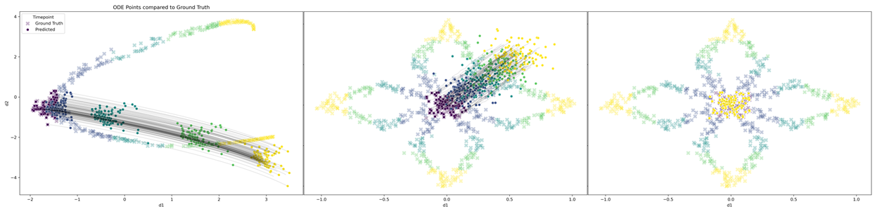
Figure 6: Trajectories with energy loss, and $\lambda_{e}=1$.

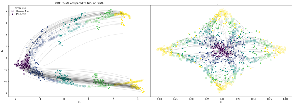
Figure 7: Trajectories with energy loss, and $\lambda_{e}=0.01$.

Ablation and hold-out

To evaluate the prediction accuracy, we train by holding-out one timepoint, and we compute the distance between the held-out sample (ground truth) and the prediction. We use the $W_{1}$, the MMD with a Gaussian kernel, and the MMD with identity map ($L^{2}$ norm between the sample means). For the Petal and Dyngen datasets, we compute the Gaussian MMD by taking the average for the scales $0.1$ and $0.5$. For the EB data, we set the scale to $1500$.

In Fig. 8, we present an ablation study for the density loss and the geodesic embedding. The parametrization was found for the model with density loss and embedding, both seem important to learn accurate trajectories. In Fig. 9, we present the trajectories when we trained by holding one timepoint out both with the embedding and density loss. In Fig. 10, we reproduce the same ablation on Dyngen data. Here, the density loss is important for the trajectories to stay on the manifold, and the embedding appears to help with the bifurcation. To complement this figure, in Tab. 6, we present the average of the KNN distance computed on the top $5\%$. On Dyngen, the trajectories with hold-out timepoints are presented in Fig. 11. Holding out the timepoint $t=3$ seems to be the hardest to learn. In Tab. 3, we show the $W_{1}$ and MMD between the predicted values and ground truth, for MIOFlow, TrajectoryNet, and DSB. For the $W_{1}$, MIOFlow is always more accurate. In Tab 4, we compare the prediction accuracy on the EB data, depending on using the GAE or not. For the GAE, we consider the choice of two kernels when computing the distance $G$; the Gaussian kernel for various bandwidth parameters, and the $\alpha$-decay kernel for different $K$-nearest neighbors. Using the GAE improves the interpolation accuracy for all metrics. We embed the data in $200$ PCA, and train the autoencoder with layers $200,100,100,50$ for $1000$ epochs. We trained the Neural ODE for $80$ epochs with $\lambda_{d}=20$, $\sigma_{t}=0.2$, linear layers of size $16,32,16,50$ with CELU activation in between layers. We train by holding out timepoint $t$ for the GAE and the neural ODE. For the MMD with the Gaussian kernel, we set the scale to $1500$.

Table 3: Leave-one-out $(t)$ $W_{1}$ and MMD with (G)aussian or (M)ean kernel between the predicted and ground truth point on the Petal and Dyngen datasets of MIOFlow, TrajectoryNet, and DSB. Lower is better.

		$t=3$			$t=4$			$t=5$
		$W_{1}$	MMD(G)	MMD(M)	$W_{1}$	MMD(G)	MMD(M)	$W_{1}$	MMD(G)	MMD(M)
Petal	MIOFlow(ours)	0.170	0.051	0.002	0.200	0.052	0.015	0.218	0.055	0.009
	TrajectoryNet	0.379	0.568	0.001	0.347	0.341	0.003	0.264	0.096	0.004
	DSB	0.310	0.386	$<$0.001	0.260	0.087	0.029	0.441	0.159	0.081
	Baseline	0.231	0.176	0.001	0.241	0.133	0.001	0.250	0.128	0.001
Dyngen	MIOFlow(ours)	0.509	0.181	0.022	1.787	0.324	3.071	1.450	0.491	1.719
	TrajectoryNet	1.797	1.125	1.588	2.953	1.450	5.790	2.185	1.037	1.913
	DSB	0.767	0.260	0.070	2.699	0.583	6.521	2.823	1.083	5.546
	Baseline	1.828	0.958	2.435	2.198	1.131	3.368	2.221	1.133	3.139

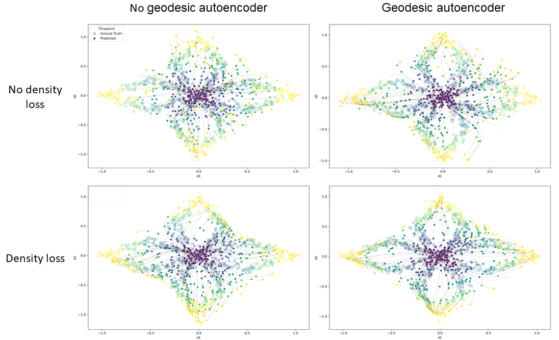
Figure 8: Petal dataset with and without the density loss (rows) or the geodesic autoencoder (columns).

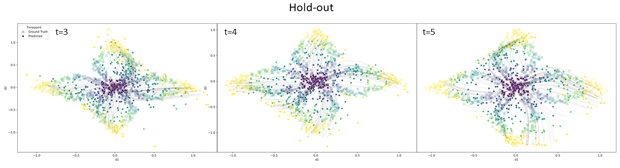
Figure 9: Trajectories for different hold-out time $t$ on the petal dataset.

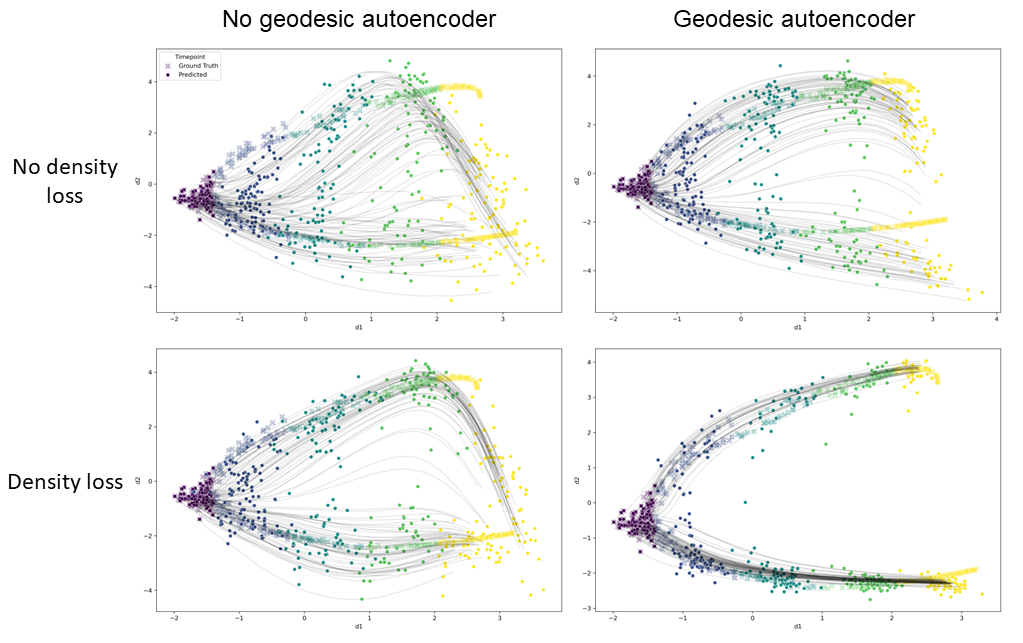
Figure 10: Dyngen dataset with and without the density loss (rows) or the geodesic autoencoder (columns).

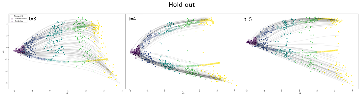
Figure 11: Trajectories for different hold-out time $t$ on the Dyngen dataset

Table 4: Leave-one-out $(t)$ $W_{1}$ and MMD with (G)aussian and (M)ean kernel between the predicted and ground truth point on the EB datasets for MIOFlow with the Gaussian, $\alpha$-decay kernel, or without GAE. Lower is better.

		$t=2$			$t=3$
GAE		$W_{1}$	MMD(G)	MMD(M)	$W_{1}$	MMD(G)	MMD(M)
$\alpha$-decay	knn $=10$	25.774	0.072	119.386	32.129	0.135	206.144
	knn $=20$	25.697	0.064	104.579	32.729	0.143	228.890
	knn $=30$	25.744	0.061	99.747	32.227	0.135	213.465
Gaussian	$\epsilon=0.05$	26.873	0.064	115.905	32.844	0.132	213.900
	$\epsilon=0.1$	26.107	0.064	109.653	32.776	0.123	203.617
	$\epsilon=0.5$	26.318	0.059	101.969	32.963	0.138	223.679
No GAE		29.243	0.063	126.608	35.709	0.119	246.609
Baseline		33.415	0.103	227.279	35.319	0.095	213.492

Nearest neighbor distance

To assist in evaluating how well the generated points land on the known manifold (ground truth points), we employ 1-NN distance from the generated points to the ground truth points. Table 5 shows the 1-NN distance for several methods and datasets. Of note is the aggregate column. Where aggregate is specified as mean, we compute the mean 1-NN distance from the predicted point to the 1-NN at the same time index. Additionally, to help reduce sensitivity due to outliers, we computed these distances and report only the mean of the worst (highest 1-NN distance) quartile, where aggregate is specified as quartile.

Table 5: Average 1-NN distance of predicted points from a given method to ground truth points at the same time label across two datasets. Rows designated mean are the average 1-NN distance, while those designated quartile are the average 1-NN distance for the worst quartile. Lower is better.

	MIOFlow(ours)	TrajectoryNet	DSB	aggregate
Petal	0.033	1.823	0.286	mean
Dyngen	0.586	2.562	1.638	mean
Petal	0.096	2.769	0.618	quartile
Dyngen	1.163	4.277	3.474	quartile

Table 6: On the Dyngen dataset, average distance of the $10$-NN for predicted points between ground truth at the same time or any. The average is computed on the highest $5\%$ observations. Lower is better.

GAE		time	any
$\alpha$-decay	knn$=5$	19.922	19.249
	knn$=10$	19.987	19.097
	knn$=15$	18.579	16.905
Gaussian	$\epsilon=0.05$	16.245	14.972
	$\epsilon=0.1$	16.245	15.491
	$\epsilon=0.5$	15.427	14.101
No GAE	Euclidean	21.589	20.486

Neural SDE

Additionally, we employed a Neural SDE from the PyTorch implementation of differentiable SDE Solvers li2020scalable,kidger2021neuralsde, and compared its results to MIOFlow (Fig. 12 & 13). We trained with a fixed diffusion function, but due to extensive training time (approximately two hours for 20 epochs for each dataset) we were unable to perform extensive hyperparameter optimization.

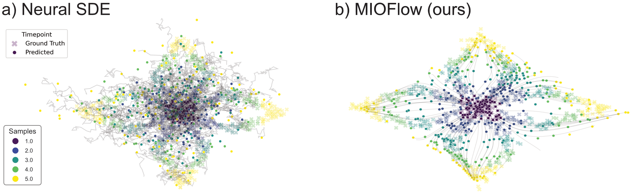
Figure 12: Comparison of Neural SDE (a) to MIOFlow (b) on the petal dataset.

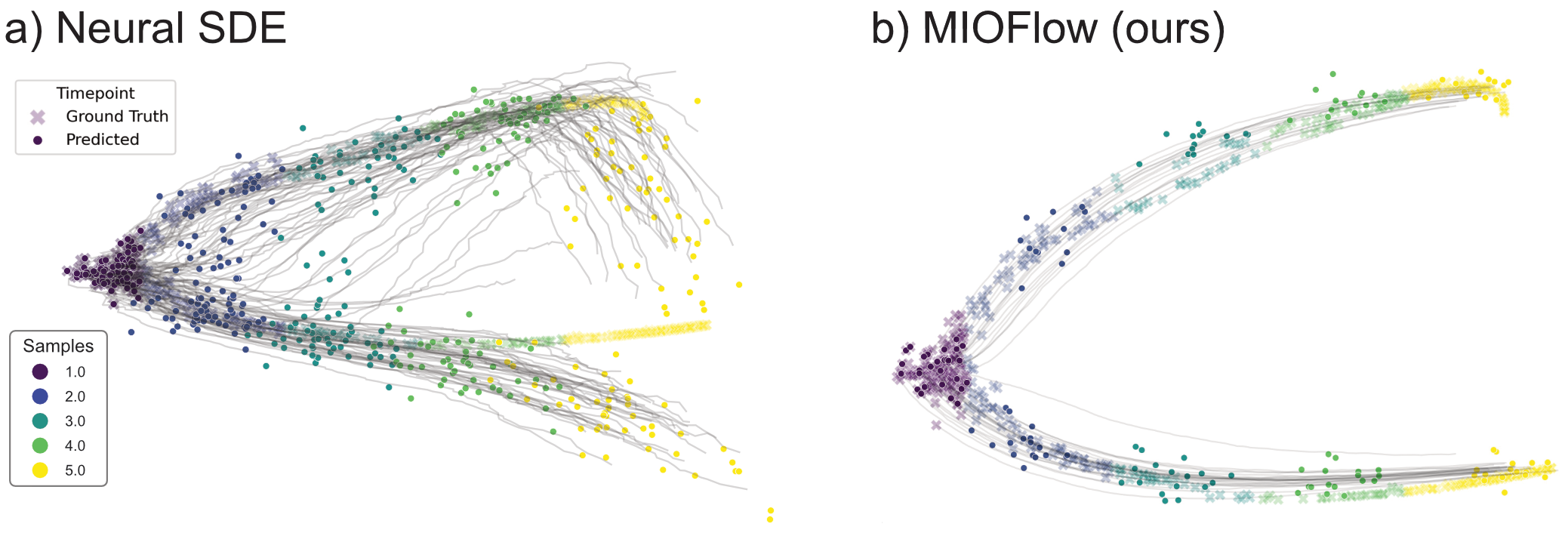
Figure 13: Comparison of Neural SDE (a) to MIOFlow (b) on the dyngen dataset.

DSB on petal

In Fig. 14, we show prediction of the DSB algorithm for different ranges of noise scale $\gamma$. With too little noise, the prediction appear to collapse on a subset of the data, while the larger scales are inaccurate for this dataset.

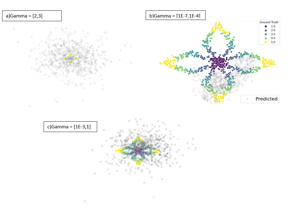
Figure 14: Comparison of DSB for different values of the noise scale $\gamma$.

Appendix D Software Versions

In Tab. 7, we present the GPU used during this work, and the following software version were used: cudatoolkit==11.1.1, graphtools==1.5.2, numpy==1.19.5, phate==1.0.7 pytorch==1.10.2, pot==0.7.0, scikit-learn==0.24.2, scipy==1.5.3, scprep==1.1.0, torchdiffeq==0.2.2, torchsde==0.2.5

Table 7: GPU specifications of High Performance Cluster. Results were generated over a swath of GPU generations and models.

Count	CPU Type	CPUs/Node	Memory/Node (GiB)	GPU Type	GPUs/Node	vRAM/GPU (GB)	Node Features
1	6240	36	370	a100	4	40	cascadelake, avx2, avx512, 6240, doubleprecision, common, bigtmp, a100
6	5222	8	181	rtx5000	4	16	cascadelake, avx2, avx512, 5222, doubleprecision, common, bigtmp, rtx5000
4	5222	8	181	rtx3090	4	24	cascadelake, avx2, avx512, 5222, doubleprecision, common, bigtmp, rtx3090
8	E5-2637_v4	8	119	gtx1080ti	4	11	broadwell, avx2, E5-2637_v4, singleprecision, common, gtx1080ti
2	E5-2660_v3	20	119	k80	4	12	haswell, avx2, E5-2660_v3, doubleprecision, common, k80

plainnat supp

References

- Agrachev and Lee [2010] Andrei Agrachev and Paul WY Lee. Continuity of optimal control costs and its application to weak kam theory. Calculus of Variations and Partial Differential Equations, 39(1):213–232, 2010.
- Belkin and Niyogi [2004] Mikhail Belkin and Partha Niyogi. Semi-Supervised Learning on Riemannian Manifolds. Machine Learning, 56(1-3):209–239, 2004.
- Benamou and Brenier [2000] Jean-David Benamou and Yann Brenier. A computational fluid mechanics solution to the Monge-Kantorovich mass transfer problem. Numerische Mathematik, 84(3):375–393, 2000.
- Bergen et al. [2021] Volker Bergen, Ruslan A. Soldatov, Peter V. Kharchenko, and Fabian J. Theis. RNA velocity—current challenges and future perspectives. Molecular Systems Biology, 17(8):e10282, 2021.
- Bunne et al. [2022] Charlotte Bunne, Laetitia Meng-Papaxanthos, Andreas Krause, and Marco Cuturi. Proximal Optimal Transport Modeling of Population Dynamics. AISTATS, 2022.
- Cannoodt et al. [2021] Robrecht Cannoodt, Wouter Saelens, Louise Deconinck, and Yvan Saeys. Spearheading future omics analyses using dyngen, a multi-modal simulator of single cells. Nature Communications, 12(1):1–9, 2021.
- Chen et al. [2018] Ricky TQ Chen, Yulia Rubanova, Jesse Bettencourt, and David K Duvenaud. Neural ordinary differential equations. Advances in Neural Information Processing Systems, 31, 2018.
- Cheng and Wu [2022] Xiuyuan Cheng and Nan Wu. Eigen-convergence of gaussian kernelized graph laplacian by manifold heat interpolation. Applied and Computational Harmonic Analysis, 61:132–190, 2022.
- Coifman and Lafon [2006] Ronald R. Coifman and Stéphane Lafon. Diffusion maps. Applied and Computational Harmonic Analysis, 21(1):5–30, 2006.
- De Bortoli et al. [2021] Valentin De Bortoli, James Thornton, Jeremy Heng, and Arnaud Doucet. Diffusion schrödinger bridge with applications to score-based generative modeling. Advances in Neural Information Processing Systems, 34, 2021.
- Duque et al. [2020] Andrés F Duque, Sacha Morin, Guy Wolf, and Kevin Moon. Extendable and invertible manifold learning with geometry regularized autoencoders. In 2020 IEEE International Conference on Big Data (Big Data), pages 5027–5036. IEEE, 2020.
- Fennell et al. [2022] Katie A Fennell, Dane Vassiliadis, Enid YN Lam, Luciano G Martelotto, Jesse J Balic, Sebastian Hollizeck, Tom S Weber, Timothy Semple, Qing Wang, Denise C Miles, et al. Non-genetic determinants of malignant clonal fitness at single-cell resolution. Nature, 601(7891):125–131, 2022.
- Finlay et al. [2020] Chris Finlay, Jörn-Henrik Jacobsen, Levon Nurbekyan, and Adam Oberman. How to train your neural ode: the world of jacobian and kinetic regularization. In International conference on machine learning, pages 3154–3164. PMLR, 2020.
- Flamary et al. [2021] Rémi Flamary, Nicolas Courty, Alexandre Gramfort, Mokhtar Z. Alaya, Aurélie Boisbunon, Stanislas Chambon, Laetitia Chapel, Adrien Corenflos, Kilian Fatras, Nemo Fournier, Léo Gautheron, Nathalie T.H. Gayraud, Hicham Janati, Alain Rakotomamonjy, Ievgen Redko, Antoine Rolet, Antony Schutz, Vivien Seguy, Danica J. Sutherland, Romain Tavenard, Alexander Tong, and Titouan Vayer. Pot: Python optimal transport. Journal of Machine Learning Research, 22(78):1–8, 2021.
- Gardiner et al. [1985] Crispin W Gardiner et al. Handbook of stochastic methods, volume 3. springer Berlin, 1985.
- Ghoussoub et al. [2021] Nassif Ghoussoub, Young-Heon Kim, and Aaron Zeff Palmer. A solution to the monge transport problem for brownian martingales. the Annals of Probability, 49(2):877–907, 2021.
- Grathwohl et al. [2019] Will Grathwohl, Ricky T. Q. Chen, Jesse Bettencourt, Ilya Sutskever, and David Duvenaud. FFJORD: Free-form Continuous Dynamics for Scalable Reversible Generative Models. In 7th International Conference on Learning Representations, 2019.
- Gretton et al. [2008] Arthur Gretton, Karsten M Borgwardt, Malte J Rasch, Bernhard Schölkopf, and Alexander Smola. A kernel method for the two-sample problem. Journal of Machine Learning Research, 1:1–10, 2008.
- Haghverdi et al. [2016] Laleh Haghverdi, Maren Büttner, F. Alexander Wolf, Florian Buettner, and Fabian J. Theis. Diffusion pseudotime robustly reconstructs lineage branching. Nature Methods, 13(10):845–848, 2016.
- Hashimoto et al. [2016] Tatsunori Hashimoto, David Gifford, and Tommi Jaakkola. Learning population-level diffusions with generative rnns. In International Conference on Machine Learning, pages 2417–2426. PMLR, 2016.
- Ho et al. [2020] Jonathan Ho, Ajay Jain, and Pieter Abbeel. Denoising Diffusion Probabilistic Models. Advances in Neural Information Processing Systems, 33:6840–6851, 2020.
- Koshizuka and Sato [2022] Takeshi Koshizuka and Issei Sato. Neural lagrangian schrödinger bridge. arXiv preprint arXiv:2204.04853, 2022.
- La Manno et al. [2018] Gioele La Manno, Ruslan Soldatov, Amit Zeisel, Emelie Braun, Hannah Hochgerner, Viktor Petukhov, Katja Lidschreiber, Maria E. Kastriti, Peter Lönnerberg, Alessandro Furlan, Jean Fan, Lars E. Borm, Zehua Liu, David van Bruggen, Jimin Guo, Xiaoling He, Roger Barker, Erik Sundström, Gonçalo Castelo-Branco, Patrick Cramer, Igor Adameyko, Sten Linnarsson, and Peter V. Kharchenko. RNA velocity of single cells. Nature, 560(7719):494–498, 2018.
- Lasry and Lions [2007] Jean-Michel Lasry and Pierre-Louis Lions. Mean field games. Japanese journal of mathematics, 2(1):229–260, 2007.
- Leeb and Coifman [2016] William Leeb and Ronald Coifman. Hölder–Lipschitz Norms and Their Duals on Spaces with Semigroups, with Applications to Earth Mover’s Distance. J Fourier Anal Appl, 22(4):910–953, 2016.
- Lei and Howard [2011] Jun Lei and Marthe J Howard. Targeted deletion of hand2 in enteric neural precursor cells affects its functions in neurogenesis, neurotransmitter specification and gangliogenesis, causing functional aganglionosis. Development, 138(21):4789–4800, 2011.
- Mathieu and Nickel [2020] Emile Mathieu and Maximilian Nickel. Riemannian continuous normalizing flows. Advances in Neural Information Processing Systems, 33:2503–2515, 2020.
- Mikami [2004] Toshio Mikami. Monge’s problem with a quadratic cost by the zero-noise limit of h-path processes. Probability theory and related fields, 129(2):245–260, 2004.
- Mikami and Thieullen [2006] Toshio Mikami and Michèle Thieullen. Duality theorem for the stochastic optimal control problem. Stochastic processes and their applications, 116(12):1815–1835, 2006.
- Mishne et al. [2019] Gal Mishne, Uri Shaham, Alexander Cloninger, and Israel Cohen. Diffusion nets. Applied and Computational Harmonic Analysis, 47(2):259–285, 2019.
- Moon et al. [2018] Kevin R. Moon, Jay S. Stanley, Daniel Burkhardt, David van Dijk, Guy Wolf, and Smita Krishnaswamy. Manifold learning-based methods for analyzing single-cell RNA-sequencing data. Current Opinion in Systems Biology, 7:36–46, 2018.
- Moon et al. [2019] Kevin R. Moon, David van Dijk, Zheng Wang, Scott Gigante, Daniel B. Burkhardt, William S. Chen, Kristina Yim, Antonia van den Elzen, Matthew J. Hirn, Ronald R. Coifman, Natalia B. Ivanova, Guy Wolf, and Smita Krishnaswamy. Visualizing structure and transitions in high-dimensional biological data. Nat Biotechnol, 37(12):1482–1492, 2019.
- Pavon et al. [2021] Michele Pavon, Giulio Trigila, and Esteban G Tabak. The data-driven schrödinger bridge. Communications on Pure and Applied Mathematics, 74(7):1545–1573, 2021.
- Peyré and Cuturi [2020] Gabriel Peyré and Marco Cuturi. Computational Optimal Transport. arXiv:1803.00567, 2020.
- Prasad et al. [2020] Neha Prasad, Karren Yang, and Caroline Uhler. Optimal transport using gans for lineage tracing. arXiv preprint arXiv:2007.12098, 2020.
- Richter-Powell et al. [2022] Jack Richter-Powell, Yaron Lipman, and Ricky TQ Chen. Neural conservation laws: A divergence-free perspective. arXiv preprint arXiv:2210.01741, 2022.
- Saelens et al. [2019] Wouter Saelens, Robrecht Cannoodt, Helena Todorov, and Yvan Saeys. A comparison of single-cell trajectory inference methods. Nature biotechnology, 37(5):547–554, 2019.
- Schiebinger et al. [2019] Geoffrey Schiebinger, Jian Shu, Marcin Tabaka, Brian Cleary, Vidya Subramanian, Aryeh Solomon, Siyan Liu, Stacie Lin, Peter Berube, Lia Lee, Jenny Chen, Justin Brumbaugh, Philippe Rigollet, Konrad Hochedlinger, Rudolf Jaenisch, Aviv Regev, and Eric S. Lander. Reconstruction of developmental landscapes by optimal-transport analysis of single-cell gene expression sheds light on cellular reprogramming. Cell, 2019.
- Singer [2006] A. Singer. From graph to manifold Laplacian: The convergence rate. Applied and Computational Harmonic Analysis, 21(1):128–134, 2006.
- Solomon et al. [2015] Justin Solomon, Fernando De Goes, Gabriel Peyré, Marco Cuturi, Adrian Butscher, Andy Nguyen, Tao Du, and Leonidas Guibas. Convolutional wasserstein distances: Efficient optimal transportation on geometric domains. ACM Transactions on Graphics (ToG), 34(4):1–11, 2015.
- Song and Ermon [2019] Yang Song and Stefano Ermon. Generative Modeling by Estimating Gradients of the Data Distribution. Advances in Neural Information Processing Systems, pages 11918–11930, 2019.
- Song et al. [2020] Yang Song, Jascha Sohl-Dickstein, Diederik P Kingma, Abhishek Kumar, Stefano Ermon, and Ben Poole. Score-based generative modeling through stochastic differential equations. In International Conference on Learning Representations, 2020.
- Street et al. [2018] Kelly Street, Davide Risso, Russell B Fletcher, Diya Das, John Ngai, Nir Yosef, Elizabeth Purdom, and Sandrine Dudoit. Slingshot: cell lineage and pseudotime inference for single-cell transcriptomics. BMC genomics, 19(1):1–16, 2018.
- Tong et al. [2020] Alexander Tong, Jessie Huang, Guy Wolf, David Van Dijk, and Smita Krishnaswamy. TrajectoryNet: A Dynamic Optimal Transport Network for Modeling Cellular Dynamics. In Proceedings of the 37th International Conference on Machine Learning, pages 9526–9536. PMLR, 2020.
- Tong et al. [2022] Alexander Tong, Guillaume Huguet, Dennis Shung, Amine Natik, Manik Kuchroo, Guillaume Lajoie, Guy Wolf, and Smita Krishnaswamy. Embedding signals on graphs with unbalanced diffusion earth mover’s distance. In ICASSP 2022-2022 IEEE International Conference on Acoustics, Speech and Signal Processing (ICASSP), pages 5647–5651, 2022.
- Tong et al. [2021] Alexander Y Tong, Guillaume Huguet, Amine Natik, Kincaid MacDonald, Manik Kuchroo, Ronald Coifman, Guy Wolf, and Smita Krishnaswamy. Diffusion earth mover’s distance and distribution embeddings. In International Conference on Machine Learning, pages 10336–10346. PMLR, 2021.
- Trapnell et al. [2014] Cole Trapnell, Davide Cacchiarelli, Jonna Grimsby, Prapti Pokharel, Shuqiang Li, Michael Morse, Niall J Lennon, Kenneth J Livak, Tarjei S Mikkelsen, and John L Rinn. Pseudo-temporal ordering of individual cells reveals dynamics and regulators of cell fate decisions. Nature biotechnology, 32(4):381, 2014.
- van der Raadt et al. [2019] Jori van der Raadt, Sebastianus HC van Gestel, Nael Nadif Kasri, and Cornelis A Albers. Onecut transcription factors induce neuronal characteristics and remodel chromatin accessibility. Nucleic acids research, 47(11):5587–5602, 2019.
- Vargas et al. [2021] Francisco Vargas, Pierre Thodoroff, Austen Lamacraft, and Neil Lawrence. Solving Schrödinger Bridges via Maximum Likelihood. Entropy, 23(9):1134, 2021.
- Villani [2009] Cédric Villani. Optimal transport: old and new, volume 338. Springer, 2009.
- Wang et al. [2021] Gefei Wang, Yuling Jiao, Qian Xu, Yang Wang, and Can Yang. Deep generative learning via schrödinger bridge. In International Conference on Machine Learning, pages 10794–10804. PMLR, 2021.
- Zhang et al. [2021] Stephen Zhang, Anton Afanassiev, Laura Greenstreet, Tetsuya Matsumoto, and Geoffrey Schiebinger. Optimal transport analysis reveals trajectories in steady-state systems. Technical report, 2021.
- Zhang and Zhang [2021] Ziqi Zhang and Xiuwei Zhang. Inference of high-resolution trajectories in single-cell RNA-seq data by using RNA velocity. Cell Reports Methods, 1(6):100095, 2021.
-
1.
For all authors…
-
(a)
Do the main claims made in the abstract and introduction accurately reflect the paper’s contributions and scope? [Yes]
-
(b)
Did you describe the limitations of your work? [Yes] In the limitations and broader impact section.
-
(c)
Did you discuss any potential negative societal impacts of your work?