Gender gaps in frontier entrepreneurship? Evidence from 1901 Oklahoma land lottery winners

Abstract

The paper investigates gender differences in entrepreneurship by exploiting a large-scale land lottery in Oklahoma at the turn of the 20${}^{\text{th}}$ century. Lottery winners claimed land in the order in which their names were drawn, so the draw number is an approximate rank ordering of lottery wealth. This mechanism allows for the estimation of a dose-response function, which relates each draw number to the expected outcome under each draw. I estimate dose-response functions on a linked dataset of lottery winners and land patent records, and find the probability of purchasing land from the government to be decreasing as a function of lottery wealth, which is evidence for the presence of liquidity constraints. I find female winners were more effective in leveraging lottery wealth to purchase additional land, as evidenced by significantly higher median dose-responses compared to those of male winners. For a sample of winners linked to the 1910 Census, I find that male winners have higher median dose-responses compared to female winners in terms of farm or home ownership. These results suggest that liquidity constraints may have been more binding for female entrepreneurs in the market economy.

Keywords: Causal inference; Entrepreneurship; Gender; Liquidity constraints; Natural experiments

1 Introduction

According to Turner (1956), “free land meant free opportunities” for settlers on the western frontier. Did settlers respond differently to these opportunities conditional on their gender? Motivated by idea that wealth shocks ought to boost entrepreneurship in the presence of liquidity constraints, the paper exploits a large-scale land lottery in Oklahoma to investigate the relationship between lottery wealth and the later entrepreneurship of lottery winners. The paper provides a window into gender constraints on economic opportunity on the frontier by further exploring whether there are gender differences in the entrepreneurial activities of winners following the lottery.

The 1901 Oklahoma land lottery opened for settlement over two million acres of land that was formerly occupied by the Kiowa, Comanche, Apache, and Wichita tribes. While previous land lotteries in Georgia were administrated by the state and had strict eligibility criteria (e.g., Poulos, 2019a), the Oklahoma lottery was administered by the federal government and any adult citizen was eligible to participate. Even though women could not legally vote at the time, they were able to participate in the Oklahoma lottery. However, eligibility was restricted to heads of household, which practically excluded married women. Female heads of household represented only 3 to 7% of the heads of household in Oklahoma at the time of the lottery (Maguire and Wiederholt, 2019). Lottery winners were required to homestead this parcel for three years to formalize their claim, unlike the Georgia land lotteries, which had no homesteading requirement.

The wealth shock produced by the Oklahoma lottery was substantial: Bohanon and Coelho (1998) estimate a lower-bound mean value estimate of $500 for each 160-acre lot at stake in the lottery, which is roughly equal to the average annual income in the state in 1900. This is an approximate mean value, and some of the lots were thought to be much more valuable: newspaper accounts at the time of the drawing indicate the most valuable lots in the district of Lawton to be worth between $20,000 to $40,000, more than 40 times the average annual income. Lottery winners claimed land in the order in which their names were drawn; thus, the draw number is an approximate rank ordering of the amount of lottery wealth in terms of the option value of the land (Bleakley and Ferrie, 2010). The rank-order drawing motivates the estimation of a dose-response function that relates each value of the dose (i.e., draw number) to the average outcome under each value of treatment. When estimating dose-response functions, observed confounding can be adjusted by modeling the outcome as a function of the treatment and a propensity score, which is the probability of receiving a treatment given observed covariates (Imbens, 2000; Hirano and Imbens, 2004).

The paper estimates the relationship between lottery wealth and the later entrepreneurship of lottery winners, as proxied by purchasing land or completing a homestead patent. I link lottery winners to land patent records to measure whether they subsequently purchased land titles though the Land Act of 1820, or filed a homestead patent through the Homestead Act (HSA) of 1862, in the decade following the lottery. In addition, I backward-link the winners to the 1900 Census to measure their pretreatment characteristics, and then forward-link to the 1910 Census to measure winners’ home or farm ownership in 1910. I hypothesize that winners with relatively low draw numbers gain more wealth in terms of the option value of the land, and are thus better able to overcome liquidity constraints and purchase additional land, file a homestead patent, or subsequently own a home or farm.

A central question of the paper is whether the estimated dose-response functions differ with respect to lottery winners’ gender. Descriptive evidence reveals gender differences in the observed probabilities of purchasing land or completing a homestead patent, with female winners less likely to engage in these entrepreneurial activities; however, after removing bias due to observed confounding, I find female winners to have a significantly higher median dose-responses than male winners. In terms of home or farm ownership in 1910, I find male winners to have a higher median dose-response than female winners. These findings suggest that for entrepreneurial activities in the market economy, liquidity constraints may have been more binding for female winners.

The political economy literature has focused on the historical origin of gender differences in labor participation (Alesina et al., 2011, 2013; Giuliano, 2015). This strand of literature contends that the type of agricultural technology adopted by societies in the preindustrial period had persistent impacts on contemporary female labor force participation and fertility. Alesina et al. (2011), for instance, show societies that traditionally practiced capital-intensive plough cultivation which relied on mainly on male workers — as opposed to labor-intensive shifting cultivation that relied on both male and female workers — have lower female participation in the workplace and in entrepreneurial activities. Historical agricultural technology is also shown to have persistent effects on fertility, sex ratios, and cultural attitudes toward women (Alesina et al., 2018; Giuliano, 2017, 2020). Qualitative evidence points to women on the western frontier as being distinctly entrepreneurial and independent due to labor shortages and the physical demands of the frontier economy (Harris, 1984; Flexner and Fitzpatrick, 1996).

Another relevant literature in economics demonstrates the importance of wealth for entrepreneurship and interprets this relationship as evidence of liquidity constraints, which restrict the ability of individuals to exchange existing wealth for other assets (e.g., Holtz-Eakin et al., 1994b; Fairlie and Krashinsky, 2012). A common empirical strategy in this literature is to determine whether an individual’s wealth affects the probability of becoming an entrepreneur; if it does, then it is evidence that liquidity constraints are present. Exogenous wealth shocks can therefore help identify the presence of liquidity constraints (Holtz-Eakin et al., 1994a). This literature frequently uses self-employment as a proxy for entrepreneurship and focuses on samples of individuals that have experienced windfall gains in terms of lottery winnings or inheritances. Lindh and Ohlsson (1996) and Blanchflower and Oswald (1998), for instance, show that the probability of being self-employed increases when people receive windfall gains in the form of lottery winnings and inheritances.

Much like recent empirical studies focused on the role of capital constraints in the historical U.S. South (Bleakley and Ferrie, 2013; González et al., 2017) and in developing countries (e.g., Banerjee et al., 2017), the present study focuses on the economic condition of capital-constrained, small-scale entrepreneurs. Gates and Bogue (1996) argue that public lands policies such as the HSA were ineffective in building wealth for small farmers because they often faced binding capital constraints. De Soto (2000) draws parallels between contemporary developing countries and the historical U.S. west, highlighting the role of formal property rights in land for transforming informal assets into collateral for loans. The outcomes used in the present study— the probability of completing a homestead or purchasing a land patents, and home or farm ownership — serve as proxies for entrepreneurship because they capture the willingness of individuals to take on risk, which is an important dimension of the environment for small entrepreneurs in developing economies (Bleakley and Ferrie, 2013).

Risk-taking has long been recognized to be one of the essential characteristics of entrepreneurship (Knight, 1921). The experimental economics literature finds strong evidence for gender differences in risk taking: in the studies surveyed by Eckel and Grossman (2008) and Croson and Gneezy (2009), women are observed to be more risk averse than men. For example, women tend to invest less in risky assets compared to men when playing investment game experiments (Charness and Gneezy, 2012). Gong and Yang (2012) find that men are less risk averse than women in both matrilineal and patrilineal societies.

The paper is organized as follows: the section immediately below reviews the historical background of the Oklahoma land lottery in the context of the broader political economy of federal land policies, and also reviews related empirical literature; Section 3 describes the data and record linkage procedure used in the study, provides summary statistics on the linked data, and results of balance tests; Section 4 describes the estimation procedure for causal dose-response relationships; Section 5 provides empirical results; Section 6 concludes.

2 Historical background and related literature

Over the course of the 19${}^{\text{th}}$ century, the public domain expanded westward as a consequence of diplomatic treaties and federal land policies such as the HSA, which opened for settlement hundreds of millions of acres of western frontier land. Any adult household head — including women, immigrants who had applied for citizenship, and freed slaves following the passage of the Fourteenth Amendment— could apply for a homestead grant of 160 acres of land, provided that they live and make improvements on the land for five years and pay a $10 filing fee.

The implicit goal of the HSA was to promote rapid settlement on the western frontier (Allen, 1991). The sparse population meant that state and local governments competed with each other to attract migrants in order to increase land values and tax revenue (Poulos, 2019b). Frontier governments offered migrants broad access to cheap land and property rights, unrestricted voting rights, and a more generous provision of schooling and other public goods (Engerman and Sokoloff, 2005). Consistent with this view, Poulos and Zeng (2021) estimate that the long-run impact of homestead policy on public school spending is equivalent to 2.5% of the total per-capita public school expenditures in 1929.

Turner’s (1956) frontier thesis posits that the frontier acted as a “safety valve” for relieving pressure from congested urban labor markets in eastern states by attracting foreign migrants and workers, many of whom were the lower end of the skill distribution. The view of the frontier as a safety valve has been explored by Ferrie (1997), who finds evidence in a linked census sample of substantial migration to the frontier by unskilled workers and considerable gains in wealth for these migrant workers. Bazzi et al. (2020) also demonstrate that frontier settlers were disproportionately illiterate and foreign-born. The authors argue that the frontier also attracted individualists who were more equipped to thrive in the harsh frontier conditions: counties with longer historical frontier experience exhibit lower contemporary property tax rates, and their citizens are more opposed to taxation and redistribution.

There were substantial barriers to entry to homesteading, and homesteaders took on enormous risk in the five years required to file a homestead patent. One of the most significant obstacles to entry was the need for capital to build a successful farming operation: contemporary writers estimated that potential homesteaders required $600 to $1000 to start a farm (Deverell, 1988). Indeed, the high cost associated with starting and maintaining a farm casts doubt on the safety valve hypothesis (Danhof, 1941). Homesteading was a risky venture: over the period of 1910 to 1919, out of 604,092 homestead entries in the U.S., totaling over 128 million acres, only 384,954 (63.7%) resulted in successful patents (Shanks, 2005).

2.1 Related empirical literature

The paper speaks to previous to empirical literature that leverages lotteried wealth to identify average causal effects of wealth on individuals’ outcomes. Poulos (2019a), for example, exploits the first two Georgia land lotteries in 1805 and 1807 to estimate the effect of winning land on subsequent officeholding and wealth. While the study finds no causal effect of wealth on the probability of candidacy or holding office, quantile regression estimates show that winning a prize in the 1805 lottery conferred lottery winners near the median of the wealth distribution a $170 increase in wealth, in terms of the estimated value of slaves owned in 1820. Bleakley and Ferrie (2013) use a sample of 1832 lottery participants linked to the full-count 1850 Census to investigate the effects of lottery prize values on the long-run wealth distribution of lottery winners, and estimate that winning a prize in the 1832 Georgia lottery significantly increases 1850 total census wealth (i.e., combined slave and real-estate wealth) by $200. The authors find that these gains were concentrated in the middle of the 1850 wealth distribution, rather than in the lower tail of the distribution where there is limited access to capital. Using the same linked sample, Bleakley and Ferrie (2016) finds no evidence of a treatment effect on the wealth, literacy, or occupational standing of lottery winners or their descendants. Using a small sample of Oklahoma lottery winners registered in Lawton and linked to both the 1900 and 1910 censuses, Bleakley and Ferrie (2010) finds that winners with lower draw numbers were more likely to remain in Oklahoma.

Several empirical studies survey lottery winners in order to estimate the effect of lottery wealth on subsequent redistributive attitudes (Doherty et al., 2006); consumption behavior and labor market earnings (Imbens et al., 2001); and bankruptcy filings (Hankins et al., 2011). In these studies, the assignment of lottery prizes is random, yet there is substantial nonresponse when surveying lottery winners to measure their attitudes or earnings, which yields a sample where the prize amount is not independent of pretreatment characteristics. The present study avoids nonresponse bias because the outcome variables are extracted from observed economic behavior such as the purchasing of land patents and from census data. However, sample bias may arise as a result of the process of linking winner records to land patent or census records with imperfect information.

2.2 Oklahoma land openings and the 1901 lottery

In the years prior to Oklahoma’s statehood in 1907, tribal lands in the central and western parts of Oklahoma were opened for settlement by the federal government to non-native American settlers. These lands were allocated by federal officials using four different mechanisms, as depicted in Figure 1: allotment, land run, lottery, and sealed bid. In 1891, the Jerome Commission reached an agreement with several tribes that transferred “surplus” tribal land to the federal government that were to be opened to settlement under the HSA (Anderson and Bearden, 1997). Most of the tribal land in central Oklahoma, which were ceded to the federal government by the Creek and Seminole Indians following the Civil War, were opened by land run beginning in 1889. Land runs were literal races to claim surveyed lots, most the size of 160 acres, with fixed starting times and locations for participants (Bohanon and Coelho, 1998). Women who participated in the land runs had to be unmarried, widowed, or legally separated from their husbands (Maguire and Wiederholt, 2019). As detailed below, the 1901 lottery randomly distributed claims to 160 acre land lots — i.e., first drawers had the first right to claim land. Prairie land in southwestern Oklahoma known as the Big Pasture was opened by first-price sealed bid auction in 1906.

About 3,250 square miles (2.08 million acres) of land in Kiowa-Comanche country — formerly occupied by the Kiowa, Comanche, Apache, and Wichita tribes — were instead opened for homestead settlement by lottery in July of 1901 and split into two districts: El Reno and Lawton. Lottery participants were required to be physically present at either the El Reno or Lawton land offices to register for the lottery, depending on whether they wished to claim land in El Reno or Lawton. El Reno had railroad access and an extra registration booth was opened to be utilized exclusively by women — 8,000 women applied at this exclusive booth and an additional 2,000 women applied at the other booths in El Reno (Anderson and Bearden, 1997). Registration was open to heads of household at least 21 years old who did not already own more than 160 acres of land. Citizenship was not required for registration, even though the drawing was initiated by the federal government. Women were allowed to participate as long as they met the above requirements.

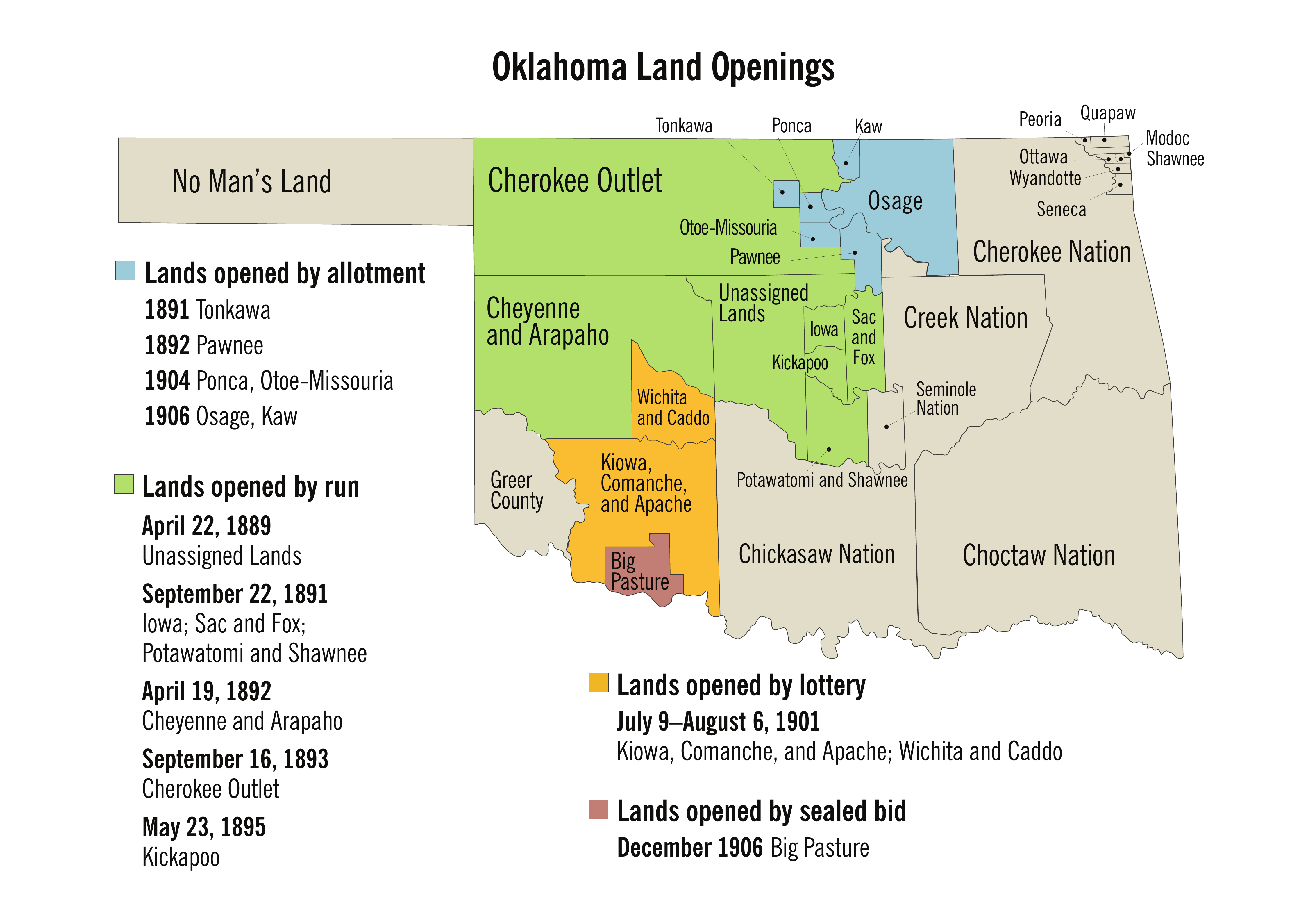
Figure 1: Oklahoma land openings. Source: Oklahoma History Center (http://www.okhistory.org/research/land).

About 170,000 people registered for the chance to win one of 13,000 lots of 160 acres in size. The lot size was not substantially smaller than 213 acres, which was the average acreage per farm in 1900 in the Oklahoma and Indian Territories at the time of the 1900 Agricultural census (Bohanon and Coelho, 1998). Federal land officials randomly drew 6,500 envelopes containing participants’ information (name, birthdate, and physical description) from each of two large hoppers — one for participants who registered in Lawton and the other for those who registered in El Reno — and envelopes were numbered as they were drawn (Anderson and Bearden, 1997). Results of the drawing were mailed to participants and posted in the newspapers. During the span of 60 days, lottery winners had the opportunity to “stake [a] claim in turn” (i.e., in the order established by the drawing) on their desired land lot according to the number on the envelope (Watson, 1988).

The lands opened by lottery contained more fertile land than the arid land in western Oklahoma opened by run. Bohanon and Coelho (1998) estimate the average value of the uncultivated lands opened by lottery was $3.10 per acre, which leads to an estimate of $496 for the 160-acre lot of uncultivated land — roughly equal to the average annual income in 1900. Given this estimate and that the chance of winning a land lot was about 7.7%, the expected value of participation was $38.19. The average value of a cultivated Oklahoma farm of 160 acres is estimated to be between $552 and $2,786. Newspaper articles written at the time of the drawing estimate that the most valuable lots in Lawton were worth between $20,000 to $40,000. These articles appeared days prior to the start of the land selection process for lottery winners, which is qualitative evidence that the location of the most valuable land lots were common knowledge. There was also weeks between the drawing and the registration of claims, so the winners would have a chance to go out into the territory and survey possible locations (Bleakley and Ferrie, 2010).

3 Data and record linkage

The analysis relies on lottery winner records, land patent records, and census data samples. First, I draw winner information from Anderson and Bearden’s (1997) list of Lawton winners and Watson’s (1988) list of El Reno winners. The records contain information on winner name, place of residence, state or territory, draw number, and for the Lawton records, the land claimed by each winner. I combine the records of El Reno and Lawton winners, and drop winners with missing draws or draw numbers that occur more than two times, which yields a sample size of $n=13837$. In the sample, 7673 winners (55.5%) registered in El Reno and had draw numbers 1 to 7731, where the Lawton records had 6164 winners (44.5%) with draw numbers 1 to 6973.

Table 1 summarizes winner characteristics at the time of registration for the 1901 lottery. In the sample, 47.4% of winners lived in Oklahoma Territory at the time of registration; 17.5% lived in Kansas; and 10.5% lived in Indian Territory. The three most frequent places lived at the time of registration were El Reno (3.8%) and Oklahoma City (2.8%), both in Oklahoma Territory, and Chickasha in Indian Territory (2.0%). I code winners’ gender by linking their first name to a public database of known female and male first names extracted from the modern census (Maiaroto, 2015). In total, 878 winners (6.3%) are identified as having female first names. Compared to male winners, female winners are more likely to have registered in El Reno, and to have lived in El Reno and the Oklahoma Territory at the time of registration. An explanation for this discrepancy is that El Reno was easier to access by railroad and women were given an exclusive booth to register.

Table 1: Summary statistics for binary pretreatment covariates and post-treatment land patent outcomes, by gender.

Variable	$\mathbf{n_{\mathrm{male}}}$	$\mathbf{\%_{\mathrm{male}}}$	$\mathbf{n_{\mathrm{female}}}$	$\mathbf{\%_{\mathrm{female}}}$	$\mathbf{n_{\mathrm{all}}}$	$\mathbf{\%_{\mathrm{all}}}$
Gender
Female	0	0.0	878	100.0	878	6.3
District of registration
Lawton	5819	44.9	345	39.3	6164	44.5
State or territory
(most frequent)
Arkansas	143	1.1	6	0.7	149	1.1
Illinois	199	1.5	5	0.6	204	1.5
Indian Territory (I.T.)	1372	10.6	86	9.8	1458	10.5
Iowa	236	1.8	12	1.4	248	1.8
Kansas	2297	17.7	127	14.5	2424	17.5
Missouri	1136	8.8	48	5.5	1184	8.6
Nebraska	137	1.1	6	0.7	143	1.0
Oklahoma Territory (O.T.)	6024	46.5	538	61.3	6562	47.4
Texas	1072	8.3	40	4.6	1112	8.0
Place of residence
(most frequent)
Anadarko, O.T.	162	1.2	8	0.9	170	1.2
Bridgeport, O.T.	104	0.8	8	0.9	112	0.8
Chickasha, I.T.	251	1.9	23	2.6	274	2.0
El Reno, O.T.	479	3.7	44	5.0	523	3.8
Enid, O.T.	158	1.2	17	1.9	175	1.3
Fort Sill, O.T.	112	0.9	8	0.9	120	0.9
Guthrie, O.T.	157	1.2	15	1.7	172	1.2
Hobart, O.T.	186	1.4	10	1.1	196	1.4
Kansas City, Missouri	141	1.1	14	1.6	155	1.1
Kingfisher, O.T.	150	1.2	23	2.6	173	1.2
Mountain View, O.T.	130	1.0	13	1.5	143	1.0
Oklahoma City, O.T.	342	2.6	45	5.1	387	2.8
Perry, O.T.	108	0.8	8	0.9	116	0.8
Shawnee, O.T.	108	0.8	5	0.6	113	0.8
Weatherford, O.T.	133	1.0	9	1.0	142	1.0
Wichita, Kansas	114	0.9	14	1.6	128	0.9
Post-treatment outcome
Land purchase	1547	11.9	80	9.1	1627	11.8
Homestead	980	7.6	28	3.2	1008	7.3

Second, I link winners to records of land patents under the Land Act of 1820, which allowed direct cash sales of public land from the General Land Office (GLO) to the public, and the HSA, issued within a decade of the 1901 drawing (Bureau of Land Management, 2017). The record linkage to land patent records is by exact match on full name (i.e., first, middle, and surname) and county/constituency (if available). Land patents are deeds transferring land ownership from the federal government to individuals, and provide information on the initial transfer of land titles from the federal government, including the patentee’s name, date of patent, and location of land.

The last two rows of Table 1 shows that among all lottery winners, 11.8% subsequently purchased land under the Land Act and 7.3% filed a homestead patent under the HSA. There are substantial gender differences in the observed outcome rates: the male-female difference is 2.8% for land purchase and 4.4% for homestead patent. I calculate Pearson correlation coefficients and find positive correlations between draw number and the probability of land purchase, 0.05 ($p<0.001$), or homestead patent, 0.07 ($p<0.001$). The positive relationship between draw number and land purchase holds for the subgroup of female winners, 0.08 ($p=0.013$), but not for the homestead outcome, -0.01 ($p=0.827$). Unlike the causal estimates presented in Section 5, these correlation coefficients include biases associated with differences in the covariates.

In order to recover post-treatment outcomes from the 1910 Census, and pretreatment characteristics of the lottery winners from the 1900 Census, I backward-link the winners to the full-count 1900 Census, and then forward-link those matched to the full-count 1910 Census. I create a sample of heads of household from the full-count 1900 and 1910 censuses. The full-count census data have only have information that is useful for genealogical inquiry transcribed, such as name, county and state of residence, age, gender, race, and birthplace. A team of undergraduate research assistants transcribed the remaining information for winners who were backward-linked to the 1900 Census and linked winners who were forward-linked to the 1900 Census. Using an automatic linking procedure described in Section LABEL:linkage, I successfully link 18.3% of 1901 winners to the 1900 Census and 16.7% of the linked sample to the 1910 Census. In comparison, Bleakley and Ferrie (2010) manually link 24.3% of Lawton winners to the 1900 Census and 33% of their linked sample to the 1910 Census.

Table LABEL:participant-census provides summary statistics on pretreatment covariates of lottery winners backward-linked to the 1900 Census ($n=2591$) and then forward-linked to the 1910 Census, for winners with non-missing farm and home ownership outcomes in 1910 ($n=397$). Since the census samples focus only on heads of household, only 1.7% of lottery winners are female and a half of a percentage of winners linked to both the 1900 and 1910 censuses are female. Similar to the statistics in Table 1, the most frequent states of residence in 1900 for lottery winners linked to either census are Kansas, Missouri, and Texas. The 1900 Census provides a richer set of demographic characteristics on the linked lottery winners: the winners skewed young, with 34.3% in the age group of 29 to 39 years old and 28.1% in the age group of 18 to 28 years old. Ninety-two percent of the winners linked to the 1900 Census are white and 7.8% are black. The 1910 Census provides information on two post-treatment outcomes of interest that capture entrepreneurial behavior: farm and home ownership. Among winners linked to both censuses, 50.6% owned a farm and 66.5% owned their own home in 1910. I calculate Pearson correlation coefficients and find no correlation between winners’ draw number and the probability of owning a farm, 0.03 ($p=0.430$), or their own home, 0.03 ($p=0.481$).

3.1 Balance tests

I assess the plausibility of the key identifying assumption (Assumption Assumption 1 defined in Section 4) that treatment level and potential outcomes are independent conditional on the observed pretreatment covariates. While this assumption is not directly testable, we can test whether there are any imbalances in the treatment levels in terms of observed covariates.

Figure 2 reports balance in the first decile of draw number in terms of the covariates used to estimate the propensity score. Specifically, I create an indicator that takes the value of one if the draw number is within the first decile and consider the first decile as the reference treatment, since lower draw numbers correspond to more lottery wealth. Each point in the plot represents a $p$ value extracted from a bivariate linear regression of the first decile indicator on each pretreatment covariate. A statistically significant coefficient on the covariate implies an imbalance in first decile of draw number in terms of that covariate.

While there is no evidence of imbalance in terms of winners’ gender, there are imbalances in terms of winners’ district of registration, state, and of place of residence at the time of registration. The indicator for winners who registered at Lawton (rather than El Reno) is below the multiplicity-corrected level of significance (dotted line). Indicators for winners from Alabama and those living in several locations in the Oklahoma Territory (e.g., Anadarko, Bridgeport, Chickasha, Hobart, and Oklahoma City) are also significant at the multiplicity-corrected level. An indicator variable for winners living in Yukon in the Oklahoma Territory is significant at the conventional level of significance (dashed line). Most (but not all) of the Oklahoma Territory locations that exhibit imbalance are geographically closer to El Reno, so it is likely that winners residing in these locations would have registered at the El Reno land office. Examining the covariate distributions by draw number decile in Table LABEL:participant-draw reveals that the percentage of winners who registered in Lawton are evenly split for the first decile of draw number, but heavily imbalanced towards El Reno in the last decile. This is due to the fact that the El Reno records had more winners, and thus higher draw numbers. Winners living in the Oklahoma Territory locations that exhibit imbalance, whom presumably registered at the El Reno office, were proportionally more likely to draw numbers in the last two deciles. By including these covariates that exhibit imbalance in the propensity score model we are able to remove the resulting bias from the causal estimands.

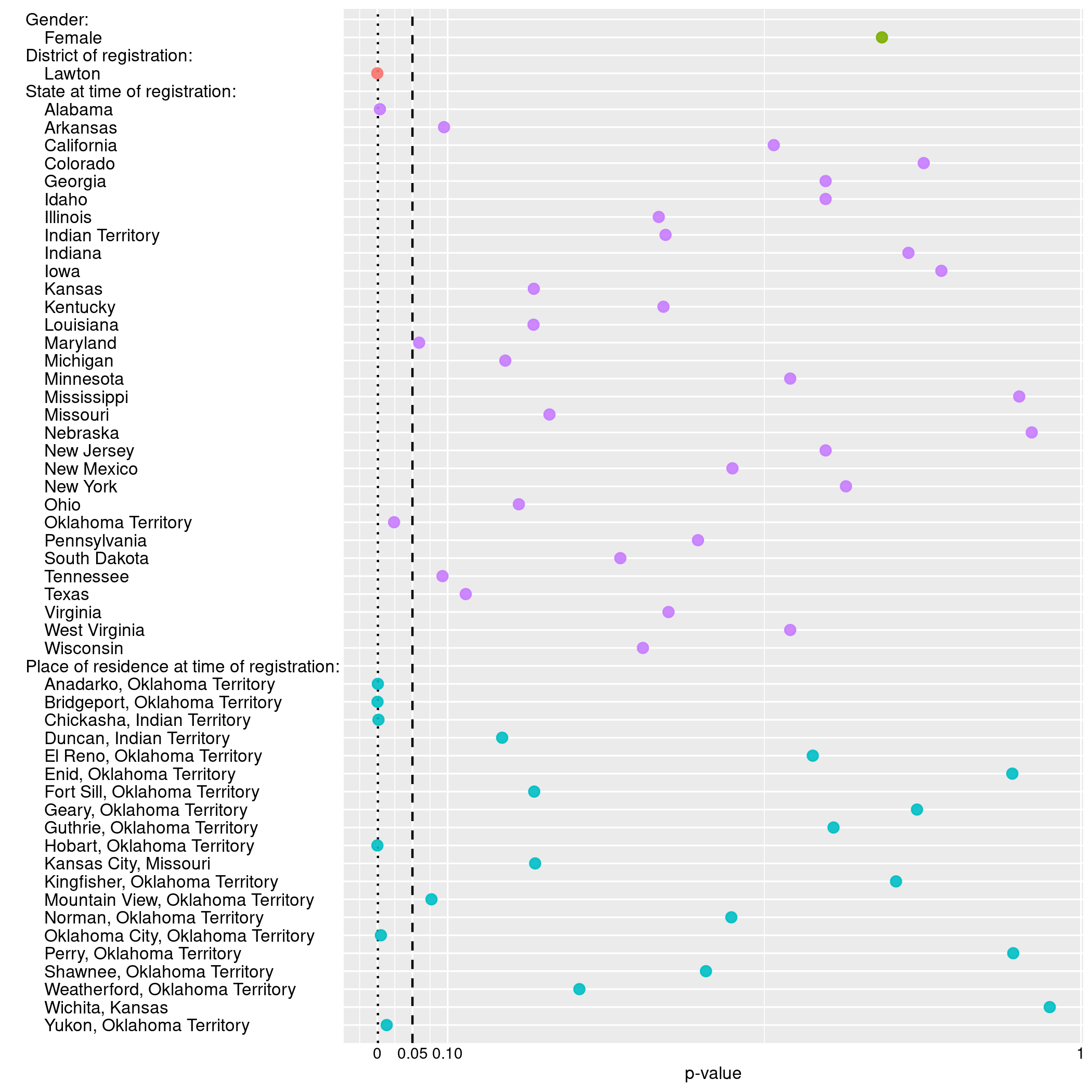
Figure 2: Balance in first draw number decile for El Reno and Lawton winners in terms of pretreatment covariates. $p$ values extracted from bivariate linear regressions of an indicator for draw number within first decile on each pretreatment covariate. The dotted vertical line is the Bonferroni corrected level of significance for 53 comparisons, $\alpha=0.0009$, whereas the dashed vertical line is $\alpha=0.05$.

4 Causal estimation

This study estimates the individual response (e.g., the probability of purchasing a land patent) that corresponds to specific values of continuous doses, i.e., random draw numbers. In the case of the Oklahoma lottery, a lower draw number corresponds to a higher dose in terms of the option value of the land. An analogy can be made to the studies of Doherty et al. and Imbens et al., where a higher amount of prize corresponds to a higher dose.

4.1 Setup

I follow the setup of Hirano and Imbens (2004) who propose estimating the entire dose-response function of a continuous treatment within the Neyman-Rubin potential outcomes framework (Neyman, 1923; Rubin, 1990). A sample of size $n$ is observed in which each lottery winner $i=\left\{1,...,n\right\}$ has been assigned to treatment level $z_{i}\in\mathcal{Z}$, where $\mathcal{Z}=\{j=1,2,\ldots,J\}$ is the collection of possible treatment levels $j$ and $\mathbf{z}$ is a length-$n$ vector of assigned treatment levels. For each winner $i$, $y_{i}$ is the realized outcome and $\bf{x}_{i}$ is a vector of pretreatment covariates. Let the binary treatment indicator $d_{i}(j)=1$ if $z_{i}=j$ and 0 otherwise. The potential outcome under treatment level $j$ is $y_{i}(j)$ and the realized outcome is $y_{i}=\sum_{j=1}^{J}d_{i}(j)y_{i}(j)$. The unit-level dose-response function is defined as the set of potential outcomes under each treatment level, $y_{i}(j):j\in\mathcal{Z}$.

A common parameter of interest is the average dose response (ADR), or the average of the unit-level dose-response function, $\mu(j)=\mathrm{E}[y_{i}(j)]$. Another common parameter is the marginal treatment effect function (Michela et al., 2011; Kreif et al., 2015), which captures the effect of increasing the treatment level by $\Delta j$ units on the expected potential outcome, $(\mathrm{E}[y_{i}(j)]-\mathrm{E}[y_{i}(j-\Delta j)])/\Delta j$. The focus in this study is on gender gaps, so interest lies in understanding the ADR function with respect to a subgroup, such as gender, defined by a subset of the covariate space, $\mathbb{C}$. A conditional marginal treatment effect function can similarly be estimated with respect to a subgroup.

Definition 1.

Conditional Average Dose Response (CADR). The average dose-response, treating $x\in\mathbb{C}$ as fixed.

$$\mu_{j,x\in\mathbb{C}}=\mathrm{E}_{{\bf x}\in\mathbb{C}}[y_{i}(j)].$$

Definition 2.

Conditional Marginal Treatment Effect (CMTE). The marginal treatment effect function, treating $x\in\mathbb{C}$ as fixed.

$$\left(\mathrm{E}_{{\bf x}\in\mathbb{C}}[y_{i}(j)]-\mathrm{E}_{{\bf x}\in\mathbb{C}}[y_{i}(j-\Delta j)]\right)/\Delta j.$$

The causal parameters can be identified under unconfoundedness, or that adjusting for observed covariates ensures independence between treatment level and potential outcomes.

Assumption 1.

Weak Unconfoundedness: $y(j)\perp\!\!\!\perp z_{i}\mid{\bf x}$,   for all $j\in\mathcal{Z}$.

The unconfoundedness assumption is weak because the conditional independence is assumed at each level of treatment rather than the joint independence of all the potential outcomes. This assumption implies that adjusting the conditional expectation of the outcome using information from the observed covariates is sufficient to remove bias from the estimate.

While it is not possible to directly test for unconfoundedness, the results of the balance tests in Figure 2 evidence imbalance in terms of some of the covariates, in particular, winners’ district of registration, state, and place of residence at the time of registration. Explicitly modeling the probability of receiving treatment as a function of covariates, and including the estimated propensity scores in the outcome model is expected to improve the consistency of the treatment effect estimates by eliminating any bias associated with differences in the observed covariates among groups of winners assigned to different treatment levels. Three additional estimation assumptions common in the causal inference literature are defined in Section LABEL:assumptions in the online supporting materials (SM).

4.2 Estimating dose-response curves

The estimation of dose-response curves involves estimating both outcome and treatment models. This estimation approach is double-robust, which requires either the treatment model or outcome model to be correctly specified to ensure consistent estimation (Kang and Schafer, 2007). Misspecification of either the treatment or outcome model can lead to bias in the estimates of the dose-response function (e.g., Poulos et al., 2022). To avoid bias resulting from model misspecification, I use the super learner (van der Laan et al., 2007; Polley and van der Laan, 2010; Polley et al., 2011) for estimating both outcome and treatment models in order to minimize the bias resulting from model misspecification. The super learner is an ensemble method that uses cross-validation to select the optimal weighted combination of many candidate classification or regression algorithms, where optimality is defined in terms of a pre-specified loss function (Kreif et al., 2015).

The first step of estimating dose-response curves is to estimate the generalized propensity score $R=r(z,{\bf x})$, which is the conditional probability a winner is assigned to each treatment level, $\mbox{Pr}(z=j\mid{\bf x}_{i})$. I estimate the generalized propensity score using the super learner estimate of winners’ draw number given the pretreatment covariates included in Table 1 for the analysis on land patent outcomes or Table LABEL:participant-census for the analysis on 1910 Census outcomes.

The second step of estimating dose response curves is to estimate the conditional expectation of the outcome as a function of the treatment level and the propensity score, $\beta(z,R)=\mathrm{E}[y\mid z=j,R=r]$ (Kreif et al., 2015). I use super learner to model the outcome as a function of continuous treatment the estimated propensity scores. Then, the ADR function can be estimated by using the estimated parameters of the outcome model to predict the average potential outcome at each level of treatment. The CADR can be estimated by averaging over winners with covariates ${\bf x}\in\mathbb{C}$; that is, the average among those having ${\bf x}\in\mathbb{C}$. As Hirano and Imbens (2004) highlight, the regression function $\beta(z,R)$ does not itself have a causal interpretation, but comparing the ADR or CADR between different levels of treatment does have a causal interpretation.

5 Empirical results

I estimate the CADR (Definition 1) and CMTE (Definition 2) on the sample of El Reno and Lawton lottery winners for the land patents outcomes, by gender subgroup. Figure 3(a) plots the relationship between draw number (1 to 6500) and the probability of purchasing land for the subgroups of male and female winners. For both groups, the expected outcomes range from about 10% to 20%, depending on draw number, which is similar to the observed (i.e., unadjusted) land purchase rate for the sample, 11.8%. The plot shows that for both male and female winners, the probability of land purchase is generally decreasing with draw number, although the relationship is non-monotonic since there is an uptick in the probability for winners with draw numbers over 6000. The negative relationship is consistent with the hypothesis that winners with relatively low draw numbers gain more wealth in terms of the option value of the land, and are thus better able to overcome liquidity constraints and purchase additional land. The non-monotonic relationship lacks a theoretical explanation since those with relatively high draw numbers got “last dibs” on the available land. Since high-drawing winners were more likely to not claim lotteried land (Bleakley and Ferrie, 2010), an explanation might be that receiving last dibs motivated them to instead purchase land from the government.

Visually comparing the CADR curves, there is a clear pattern of gender differences in terms of land patent purchases, with female winners actually more likely to purchase land compared to male winners. I conduct a Mann-Whitney U test to see if the mean ranks (which approximate the median) of the dose-response curves differ based on gender, resulting in a two-sided test $p$-value of less than 0.001, which is evidence against the null hypothesis that the CADR functions for male and female winners are equal. The Hodges-Lehmann estimate and 95% confidence interval indicates that the median of the dose-response curve for female winners is 1.74 [1.68, 1.80] percentage points higher than the median for male winners.

Figure 3(b) provides estimates of the CMTE, which captures the effect of increasing the draw number by $\Delta j=1000$ on the probability of land purchase for the gender subgroups. This parameter has a causal interpretation because it compares the expected potential outcomes under different levels of treatment; for instance, the difference in the expected potential outcomes under draw number 1001 and number 1, number 1002 and number 2, and so on. The CMTE point estimates are generally decreasing as a function of draw number until about the 6000${}^{\text{th}}$ draw, which implies that increasing the draw number has a negative incremental effect on the expected probability of purchasing land. For instance, the incremental causal effect of increasing the draw number from 25 to 1025 decreases the probability of purchasing land by 0.002 [-0.00001, -0.004] percentage points for male winners and 0.003 [-0.001, -0.004] for female winners. While the negative causal effects are consistent with the liquidity constraint hypothesis, the finding of positive causal effects for winners on the right-tail of the curve lacks theoretical explanation. For instance, the incremental effect of increasing the draw number from 5058 to 6058 increases the probability of land purchase for both subgroups by 0.001 [0.001, 0.002] percentage points. These are very small incremental effects considering the observed land purchase rate is 11.8%.

(a) Average dose-response function

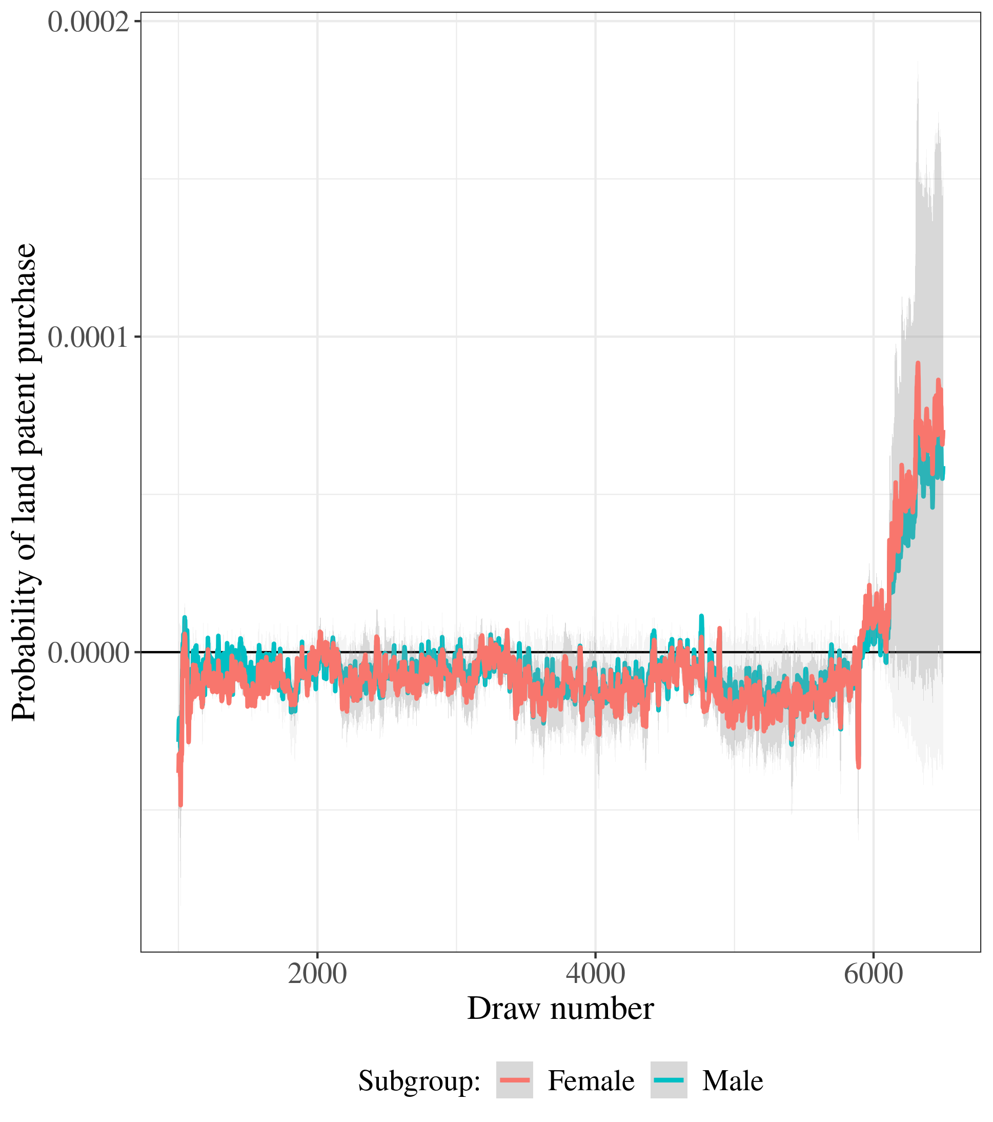
(b) Marginal treatment effect function

Figure 3: Estimated CADR (a) and CMTE (b) for the land patent purchase outcome. The solid lines represent the estimated values by gender subgroup and the shaded regions represent 95% confidence intervals calculated using the standard deviation of the predictions from all candidate algorithms in the super learner. The darker shaded regions correspond to the female subgroup.

When the outcome is probability of completing a homestead patent within ten years following the 1901 lottery, the estimated CADR curves for male and female winners are relatively flat as a function of draw number, as shown in Figure 4(a). For each group, the probability of completing a homestead ranges from about 5% to 10%, which is similar to the observed rate of 7.3%. Results of a Mann-Whitney U test for difference between CADR curves demonstrate the median dose-response for female winners is 0.09 [0.08, 0.10] percentage points higher than the median for male winners — a substantially smaller median difference compared to the land patent purchase outcome. Figure 4(b), which plots the CMTE function, shows both negative or positive incremental effects, depending on the draw number. For example, the incremental effect of moving from draw number 60 to 1060 yields for male winners a 0.002 [0.00002, 0.004] percentage point decrease in the probability of completing a homestead and a 0.001 [0.0003, 0.002] decrease for female winners. These are very small incremental effects compared to the observed rate completing a homestead for the sample.

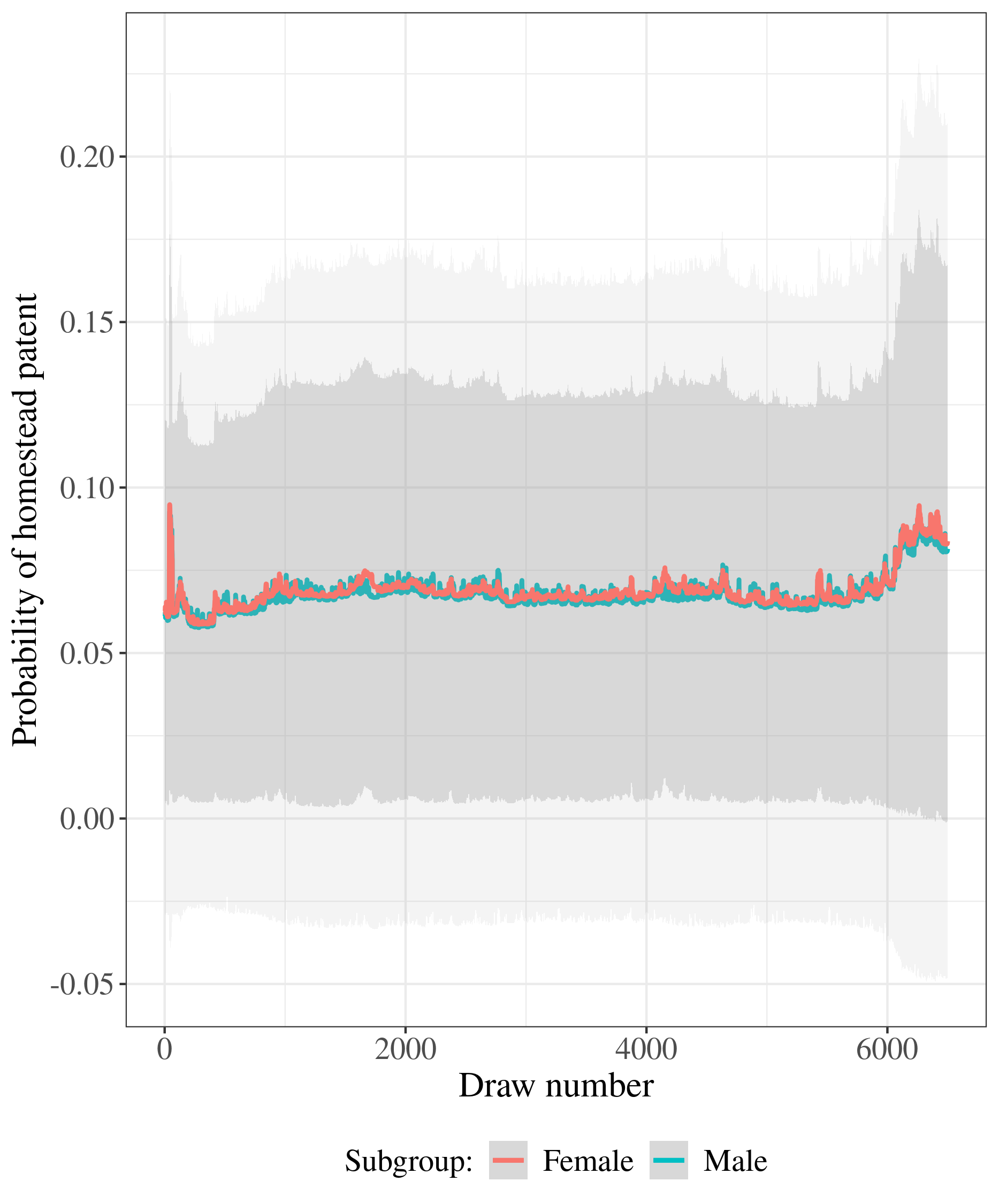
(a) Average dose-response function

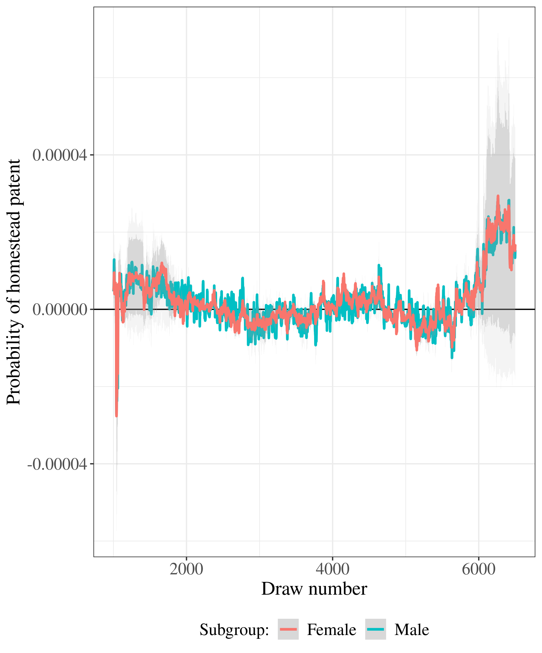
(b) Marginal treatment effect function

Figure 4: Estimated CADR (a) and CMTE (b) for the homestead patent outcome. See notes to Figure 3.

Figures LABEL:farm-plots and LABEL:home-plots report the estimated CADR functions on the probability of owning a farm or home in 1910, respectively, for the sample backward linked to the 1900 Census and forward-linked to the 1910 Census. Visually, there is no clear relationship between draw number and the expected probability of owning a farm or a home in 1910, for either gender subgroup. Male winners are more likely than female winners to own a farm in 1910 compared to female winners: the estimated median difference between the CADR functions is 1.54 [1.51, 1.57] percentage points higher for male winners. This is a relatively large difference, considering that the observed rate of farm ownership for the sample is 66.5%. Male winners are also more likely to own a home in 1910 compared to female winners, with a median difference of 2.64 [2.58, 2.69], which is also a substantial difference considering the observed rate of home ownership in the entire sample is 50.6%. The CMTE functions show incremental treatment effects on the probability of farm or home ownership that are practically zero.

6 Conclusion

There is substantial empirical evidence in economics pointing to (i.) gender differences in risk taking, which is an important element of entrepreneurship; and (ii.), the importance of wealth for entrepreneurship, which implies that liquidity constraints are present. However, not much is known about whether there are gender differences in the relationship between wealth and entrepreneurship, or how liquidity constraints impact entrepreneurial behavior conditional on gender.

The results of the paper can be interpreted as evidence of the presence of liquidity constraints among mostly white and male settlers on the western frontier. For both female and male lottery winners, the probability of purchasing land under the Land Act of 1820 subsequent to the lottery drawing is a declining function of the draw number. This finding indicates that those with more lottery wealth were more likely to buy land than those with less lottery wealth, and implies that liquidity constraints were present at the time of the lottery. Surprisingly, female winners have a higher dose-response curve than male winners, with a median difference of 1.74 [1.68, 1.80] percentage points, which suggests female winners were better able to leverage their lottery wealth into subsequent land purchases. This is a relative large median difference, considering the rate of land patent purchase is about 12%. Female winners also have a higher dose-response in terms of completing a homestead, although the median difference is much smaller, 0.09 [0.08, 0.10]. For a much smaller sample of winners linked to the 1900 and 1910 censuses, I find that the median dose-response for male winners to be 1.54 [1.51, 1.57] percentage points higher than for female winners, and 2.64 [2.58, 2.69] higher in terms of the home ownership outcome. These are substantial differences relative to the observed rates of farm and ownership for the entire sample.

Together, these findings suggest female winners were able to overcome liquidity constraints and either purchase additional land from the government or file a homestead patent. Both of these entrepreneurial activities were made possible by the federal government, with few restrictions on female participation. At the same time, there is evidence that men had the advantage in entrepreneurial activities in the market economy, such as home and farm ownership. These results suggest that liquidity constraints may have been comparatively more binding for female entrepreneurs in the market economy.

References

- Alesina et al. (2011) Alesina, A., P. Giuliano, and N. Nunn (2011). Fertility and the plough. American Economic Review 101(3), 499–503.
- Alesina et al. (2013) Alesina, A., P. Giuliano, and N. Nunn (2013). On the origins of gender roles: Women and the plough. The Quarterly Journal of Economics 128(2), 469–530.
- Alesina et al. (2018) Alesina, A., P. Giuliano, and N. Nunn (2018). Traditional agricultural practices and the sex ratio today. PloS one 13(1), e0190510.
- Allen (1991) Allen, D. W. (1991). Homesteading and property rights; or, “How the West was really won”. The Journal of Law and Economics 34(1), 1–23.
- Anderson and Bearden (1997) Anderson, J. K. and S. E. Bearden (1997). Kiowa-Comanche-Apache land opening 1901, homestead entry listing : Lawton District. Lawton, OK: Museum of the Great Plains.
- Banerjee et al. (2017) Banerjee, A. V., E. Breza, E. Duflo, and C. Kinnan (2017). Do credit constraints limit entrepreneurship? Heterogeneity in the returns to microfinance. Global Poverty Research Lab Working Paper No. 17-104, Available at http://dx.doi.org/10.2139/ssrn.3126359.
- Bazzi et al. (2020) Bazzi, S., M. Fiszbein, and M. Gebresilasse (2020). Frontier culture: The roots and persistence of “rugged individualism” in the United States. Econometrica 88(6), 2329–2368.
- Blanchflower and Oswald (1998) Blanchflower, D. G. and A. J. Oswald (1998). What makes an entrepreneur? Journal of labor Economics 16(1), 26–60.
- Bleakley and Ferrie (2010) Bleakley, H. and J. Ferrie (2010). Shocking behavior: Land lotteries in 1832 Georgia and 1901 Oklahoma and later life outcomes. Available at https://users.nber.org/~confer/2010/CS10/Bleakley_Ferrie.pdf.
- Bleakley and Ferrie (2016) Bleakley, H. and J. Ferrie (2016). Shocking behavior: Random wealth in antebellum Georgia and human capital across generations. The Quarterly Journal of Economics.
- Bleakley and Ferrie (2013) Bleakley, H. and J. P. Ferrie (2013). Up from poverty? The 1832 Cherokee Land Lottery and the long-run distribution of wealth. National Bureau of Economic Research. Available at https://www.nber.org/papers/w19175.
- Bohanon and Coelho (1998) Bohanon, C. E. and P. R. Coelho (1998). The costs of free land: The Oklahoma land rushes. The Journal of Real Estate Finance and Economics 16(2), 205–221.
- Bureau of Land Management (2017) Bureau of Land Management (2017). General Land Office (GLO) Records Automation. Washington, DC: Bureau of Land Management. Available at: https://glorecords.blm.gov/.
- Charness and Gneezy (2012) Charness, G. and U. Gneezy (2012). Strong evidence for gender differences in risk taking. Journal of Economic Behavior & Organization 83(1), 50–58.
- Croson and Gneezy (2009) Croson, R. and U. Gneezy (2009). Gender differences in preferences. Journal of Economic Literature 47(2), 448–74.
- Danhof (1941) Danhof, C. H. (1941). Farm-making costs and the “safety valve”: 1850-60. Journal of Political Economy 49(3), 317–359.
- De Soto (2000) De Soto, H. (2000). The mystery of capital: Why capitalism triumphs in the West and fails everywhere else. New York, NY: Basic books.
- Deverell (1988) Deverell, W. F. (1988). To loosen the safety valve: Eastern workers and western lands. The Western Historical Quarterly 19(3), 269–285.
- Doherty et al. (2006) Doherty, D., A. S. Gerber, and D. P. Green (2006). Personal income and attitudes toward redistribution: A study of lottery winners. Political Psychology 27(3), 441–458.
- Eckel and Grossman (2008) Eckel, C. C. and P. J. Grossman (2008). Men, women and risk aversion: Experimental evidence. Handbook of Experimental Economics Results 1, 1061–1073.
- Engerman and Sokoloff (2005) Engerman, S. L. and K. L. Sokoloff (2005). The evolution of suffrage institutions in the New World. The Journal of Economic History 65(4), 891–921.
- Evans and Jovanovic (1989) Evans, D. S. and B. Jovanovic (1989). An estimated model of entrepreneurial choice under liquidity constraints. Journal of Political Economy 97(4), 808–827.
- Evans and Leighton (1989) Evans, D. S. and L. S. Leighton (1989). Some empirical aspects of entrepreneurship. The American Economic Review 79(3), 519–535.
- Fairlie and Krashinsky (2012) Fairlie, R. W. and H. A. Krashinsky (2012). Liquidity constraints, household wealth, and entrepreneurship revisited. Review of Income and Wealth 58(2), 279–306.
- Ferrie (1997) Ferrie, J. P. (1997). Migration to the frontier in mid-nineteenth century America: A re-examination of Turner’s ‘safety valve’. Available at: http://faculty.wcas.northwestern.edu/~fe2r/papers/munich.pdf.
- Flexner and Fitzpatrick (1996) Flexner, E. and E. F. Fitzpatrick (1996). Century of struggle: The woman’s rights movement in the United States. Cambridge, MA: Harvard University Press.
- Gates (1936) Gates, P. W. (1936). The homestead law in an incongruous land system. The American Historical Review 41(4), 652–681.
- Gates and Bogue (1996) Gates, P. W. and A. G. Bogue (1996). The Jeffersonian dream: Studies in the history of American land policy and development. Albuquerque, NM: University of New Mexico Press.
- Giuliano (2015) Giuliano, P. (2015). The role of women in society: From preindustrial to modern times. CESifo Economic Studies 61(1), 33–52.
- Giuliano (2017) Giuliano, P. (2017). Gender: An historical perspective. Working Paper 23635, National Bureau of Economic Research.
- Giuliano (2020) Giuliano, P. (2020). Gender and culture. Oxford Review of Economic Policy 36(4), 944–961.
- Gong and Yang (2012) Gong, B. and C.-L. Yang (2012). Gender differences in risk attitudes: Field experiments on the matrilineal Mosuo and the patriarchal Yi. Journal of Economic Behavior & Organization 83(1), 59–65.
- González et al. (2017) González, F., G. Marshall, and S. Naidu (2017). Start-up nation? Slave wealth and entrepreneurship in Civil War Maryland. The Journal of Economic History 77(2), 373–405.
- Hankins et al. (2011) Hankins, S., M. Hoekstra, and P. M. Skiba (2011). The ticket to easy street? The financial consequences of winning the lottery. Review of Economics and Statistics 93(3), 961–969.
- Harris (1984) Harris, K. (1984). Sex roles and work patterns among homesteading families in northeastern colorado, 1873-1920. Frontiers: A Journal of Women Studies, 43–49.
- Hirano and Imbens (2004) Hirano, K. and G. W. Imbens (2004). The propensity score with continuous treatments. Applied Bayesian Modeling and Causal Inference from Incomplete-Data Perspectives: An Essential Journey with Donald Rubin’s Statistical Family, 73–84.
- Holtz-Eakin et al. (1994a) Holtz-Eakin, D., D. Joulfaian, and H. S. Rosen (1994a). Entrepreneurial decisions and liquidity constraints. The RAND Journal of Economics, 334–347.
- Holtz-Eakin et al. (1994b) Holtz-Eakin, D., D. Joulfaian, and H. S. Rosen (1994b). Sticking it out: Entrepreneurial survival and liquidity constraints. Journal of Political Economy 102(1), 53–75.
- Homola et al. (2023) Homola, J., C. Huff, Y. Nishimura, and A. Times (2023). The gendered legacies of the frontier and military enlistment behavior. Journal of Historical Political Economy 2(4).
- Imbens (2000) Imbens, G. W. (2000). The role of the propensity score in estimating dose-response functions. Biometrika, 706–710.
- Imbens et al. (2001) Imbens, G. W., D. B. Rubin, and B. I. Sacerdote (2001). Estimating the effect of unearned income on labor earnings, savings, and consumption: Evidence from a survey of lottery players. American Economic Review 91(4), 778–794.
- Kang and Schafer (2007) Kang, J. D. and J. L. Schafer (2007). Demystifying double robustness: A comparison of alternative strategies for estimating a population mean from incomplete data. Statistical Science, 523–539.
- Knight (1921) Knight, F. H. (1921). Risk, Uncertainty and Profit. New York, NY: Houghton Mifflin.
- Kreif et al. (2015) Kreif, N., R. Grieve, I. Díaz, and D. Harrison (2015). Evaluation of the effect of a continuous treatment: a machine learning approach with an application to treatment for traumatic brain injury. Health Economics 24(9), 1213–1228.
- Levine and Rubinstein (2017) Levine, R. and Y. Rubinstein (2017). Smart and illicit: Who becomes an entrepreneur and do they earn more? The Quarterly Journal of Economics 132(2), 963–1018.
- Lindh and Ohlsson (1996) Lindh, T. and H. Ohlsson (1996). Self-employment and windfall gains: Evidence from the swedish lottery. The Economic Journal, 1515–1526.
- Maguire and Wiederholt (2019) Maguire, K. and B. Wiederholt (2019). 1889 Oklahoma land run: the settlement of Payne County. Journal of Family History 44(1), 52–69.
- Maiaroto (2015) Maiaroto, T. (2015). Social harvest. https://github.com/SocialHarvest/harvester/tree/master/data.
- Michela et al. (2011) Michela, B., M. Alessandra, et al. (2011). Nonparametric estimators of dose-response functions. Technical report, Luxembourg Institute of Socio-Economic Research (LISER). Available at: https://liser.elsevierpure.com/fr/publications/nonparametric-estimators-of-dose-response-functions.
- Neyman (1923) Neyman, J. (1923). On the application of probability theory to agricultural experiments. Annals of Agricultural Sciences 51(1). Reprinted in Splawa-Neyman et al. (1990).
- Polley et al. (2011) Polley, E. C., S. Rose, and M. J. van der Laan (2011). Super learning. In Targeted learning, pp. 43–66. Springer.
- Polley and van der Laan (2010) Polley, E. C. and M. J. van der Laan (2010). Super learner in prediction. U.C. Berkeley Division of Biostatistics Working Paper Series. Working Paper 266. Available at: https://biostats.bepress.com/ucbbiostat/paper266.
- Poulos (2019a) Poulos, J. (2019a). Land lotteries, long-term wealth, and political selection. Public Choice 178(1), 217–230.
- Poulos (2019b) Poulos, J. (2019b). State-building through public land disposal? An application of matrix completion for counterfactual prediction. arXiv preprint arXiv:1903.08028.
- Poulos et al. (2022) Poulos, J., M. Horvitz-Lennon, K. Zelevinsky, T. Huijskens, P. Tyagi, J. Yan, J. Diaz, T. Cristea-Platon, and S.-L. Normand (2022). Targeted learning in observational studies with multi-level treatments: An evaluation of antipsychotic drug treatment safety. arXiv preprint arXiv:2206.15367.
- Poulos and Zeng (2021) Poulos, J. and S. Zeng (2021). RNN-based counterfactual prediction, with an application to homestead policy and public schooling. Journal of the Royal Statistical Society: Series C (Applied Statistics) 70(4), 1124–1139.
- Rubin (1990) Rubin, D. B. (1990). Comment: Neyman (1923) and causal inference in experiments and observational studies. Statistical Science 5(4), 472–480.
- Schumpeter (1934) Schumpeter, J. (1934). The Theory of Economic Development. Cambridge, MA: Harvard University Press.
- Shanks (2005) Shanks, T. R. (2005). The homestead act: A major asset-building policy in american history.
- Splawa-Neyman et al. (1990) Splawa-Neyman, J., D. Dabrowska, T. Speed, et al. (1990). On the application of probability theory to agricultural experiments. essay on principles. section 9. Statistical Science 5(4), 465–472.
- Turner (1956) Turner, F. J. (1956). The Significance of the Frontier in American History. Ithaca, NY: Cornell University Press.
- van der Laan et al. (2007) van der Laan, M. J., E. C. Polley, and A. E. Hubbard (2007). Super learner. Statistical Applications in Genetics and Molecular Biology 6(1).
- Watson (1988) Watson, L. S. (1988). Names of the El Reno Land District, Homesteader Filings, 1902. Guthrie, OK.: H.H. Edwards.