Minimum Weight Euclidean -Spanners††thanks: A preliminary version of this paper appears in the Proceedings of the 48th International Workshop on Graph-Theoretic Concepts in Computer Science (WG), LNCS, Springer, 2022.
Abstract
Given a set of points in the plane and a parameter , a Euclidean -spanner is a geometric graph that contains, for all , a -path of weight at most . We show that the minimum weight of a Euclidean -spanner for points in the unit square is , and this bound is the best possible. The upper bound is based on a new spanner algorithm in the plane. It improves upon the baseline , obtained by combining a tight bound for the weight of a Euclidean minimum spanning tree (MST) on points in , and a tight bound for the lightness of Euclidean -spanners, which is the ratio of the spanner weight to the weight of the MST. Our result generalizes to Euclidean -space for every constant dimension : The minimum weight of a Euclidean -spanner for points in the unit cube is , and this bound is the best possible.
For the section of the integer lattice in the plane, we show that the minimum weight of a Euclidean -spanner is between and . These bounds become and when scaled to a grid of points in the unit square. In particular, this shows that the integer grid is not an extremal configuration for minimum weight Euclidean -spanners.
Keywords: Euclidean spanner, minimum weight, integer lattice, Yao-graph
1 Introduction
For a set of points in a metric space and a parameter , a graph is a -spanner if contains, between every two points , a -path of weight at most , where denotes the distance between and . In other words, a -spanner distorts the true distances between any pair of points up to a factor ; the parameter is the stretch factor of the spanner. Several optimization criteria have been considered for -spanners, such as the size (number of edges), the weight (sum of edge weights), the maximum degree, and the hop-diameter. Specifically, the sparsity of a spanner is the ratio between the number of edges and vertices; and the lightness is the ratio between the weight of a spanner and the weight of a minimum spanning tree (MST) on .
In this paper, we focus on the Euclidean -space in constant dimension . In this case, for every constant , there exist -spanners with sparsity and lightness that depends only on and . The precise dependence on (assuming constant dimension ) has almost completely been determined: Every finite point set in admits a Euclidean -spanner with sparsity and lightness. The sparsity bound is the best possible, and the lightness bound is tight up to the factor [40]. Several classical spanner constructions achieve sparsity in such as Yao-graphs [6, 16, 48, 52], -graphs [36, 37], gap-greedy spanners [7] and path-greedy spanners [6]; see the book by Narasimhan and Smid [45] and the more recent surveys surveys [31, 44]. For lightness, Das et al. [17, 19, 45] were the first to construct -spanners of lightness in Euclidean -space. This bound has been generalized to metric spaces with doubling dimension , see [10, 30, 25]. Recently, Le and Solomon [40] showed that the path-greedy -spanner in has lightness ; and so the same spanner achieves a tight bound for sparsity and an almost tight bound for lightness.
Lightness versus Minimum Weight.
Lightness is a convenient optimization parameter for a spanner on a finite point set , as it is invariant under similarities (i.e., dilations, rotations, and translations). It also provides an approximation ratio for the minimum weight -spanner on , as the weight of a Euclidean MST (for short, EMST) of is a trivial lower bound on the spanner weight. For points in the unit cube , the weight of the EMST is , and this bound is the best possible [24, 50]. In particular, a suitably scaled section of the integer lattice attains this bound up to constant factors (in every constant dimension ). Supowit et al. [51] proved similar bounds for the minimum weight of other popular graphs, such as spanning cycles and perfect matchings on points in the unit cube .
The combination of the current best bounds on lightness and the weight of an EMST implies that every set of points in admits a Euclidean -spanner of weight
| (1) |
However, the lower bound constructions for the two (almost) tight upper bounds are very different: The lightness lower bound holds for the union of -dimensional grids on two opposite facets of a unit cube [40], and the bound on EMST holds for a -dimensional grid in a unit cube [24]. It turns out that these upper bounds cannot be attained simultaneously. In fact, the bound (1) can be improved to
| (2) |
for every constant , and (2) is tight (Theorem 1). The improvement is most prominent in the plane: from to .
Contributions.
We obtain a tight upper bound on the minimum weight of a Euclidean -spanner for points in .
Theorem 1.
For every constant and , every set of points in the unit cube admits a Euclidean -spanner of weight , and this bound is the best possible.
The upper bound is established by a new spanner algorithm, SparseYao, that modifies the classical Yao-graph construction using novel geometric insight (Section 3). The weight analysis is based on a charging scheme that charges the weight of the spanner to empty regions (Section 4). The lower bound construction is a lattice generated by orthogonal vectors of weight and (Section 2); rather than a square grid.
A section of the integer lattice is the extremal configuration for many problems in combinatorial geometry (e.g., minimum-weight EMST, as noted above). Surprisingly, the minimum weight of Euclidean -spanners for such a grid is still not known. We provide the first nontrivial upper and lower bounds in the plane.
Theorem 2.
For every , the minimum weight of a -spanner for the section of the integer lattice is between and .
When scaled to points in the unit square , the upper bound confirms that a square grid does not maximize the minimum weight of Euclidean -spanners.
Corollary 3.
For every , the minimum weight of a -spanner for points in a scaled section of the integer grid in is between and .
The lower bound is derived from an elementary criterion (the empty slab condition) for an edge to be present in every -spanner (Section 2). The upper bound is based on analyzing the SparseYao algorithm from Section 3, combined with number theoretic results on Farey sequences (Section 6). Closing the gap between the lower and upper bounds in Theorem 2 remains an open problem. Higher dimensional generalizations are also left for future work. In particular, multidimensional variants of Farey sequences are currently not well understood.
Further Related Previous Work.
Many algorithms have been developed for constructing Euclidean -spanners for points in [1, 14, 17, 18, 19, 23, 30, 32, 41, 43, 46], each designed for one or more optimization criteria (such as lightness, sparsity, hop diameter, maximum degree, or running time). See [31, 44, 45] for comprehensive surveys. We briefly review previous constructions pertaining to the minimum weight for points in the unit cube , where the weight of an EMST is .
The path-greedy spanner algorithm [6] (abbreviated as “greedy”) generalizes Kruskal’s MST algorithm: Given and points in a metric space, it sorts the edges of the complete graph on the points by nondecreasing weight, and incrementally constructs a spanner starting from the empty graph; it adds an edge to the spanner if does not already contain an -path of weight at most . As noted above, Le and Solomon [40] recently proved that for points in the unit cube, the greedy algorithm returns a -spanner of weight . This bound is weaker than Theorem 1 for points arranged in a grid, for example, but it is unclear whether the analysis of the greedy spanner can be improved to match the tight bound in Theorem 1.
A classical method for constructing a -spanners uses well-separated pair decompositions (WSPD) with a hierarchical clustering; see [33, Chap. 3]. Due to a hierarchy of depth , this technique has been adapted broadly to dynamic, kinetic, and reliable spanners [13, 14, 29, 47]. However, the weight of the resulting -spanner for points in is [29]. The factor is due to the depth of the hierarchy; and it cannot be removed for any spanner with hop-diameter [3, 20, 49].
Several constructions for -spanners combine hierarchical clustering with a greedy approach [18, 32] (either using approximate distances or running a greedy algorithm on a hierarchical spanner). These “approximate” greedy spanners achieve lightness in Euclidean -space, hence weight for points in . They have been generalized to doubling metrics with the same lightness bound [10, 25, 30].
Yao-graphs and -graphs are geometric proximity graphs, defined in the plane as follows. For a constant , consider cones of aperture around each point ; in each cone, connect to a “closest” point . The two graphs (Yao-graphs and -graphs) differ in the metric used for measuring the distance from to : For Yao-graphs, minimizes the Euclidean distance from to , and for -graphs minimizes the distance from to the orthogonal projection of to the angle bisector of the cone. Both constructions generalize to , for all , where the number of cones is . For -graphs, the computation of closest points reduces to orthogonal range searching queries (rather than circular disk ranges for Yao-graphs), and a -graph for points in can be computed in time [45, Sec. 5.5]. Both - and Yao-graphs are -spanners if , and this bound cannot be improved [6, 37, 45, 48]. Finding the optimal constant factors hidden in the notation is an active area of research [4, 5, 8, 11, 12]. However, if we place and equally spaced points on opposite sides of the unit square, then the weight of both Yao- and -graphs with parameter will be , which substantially exceeds the bound in Theorem 1 for any fixed as .
Optimizing various parameters of Euclidean spanners on the integer lattice is a natural problem. Previous work determined the minimum stretch factor in terms of the maximum degree for small values of . There exist Euclidean -spanners for with maximum degree , and -spanners with ; and these bounds are the best possible [22, 28].
Organization.
We start with our lower bound constructions (Section 2) as a warm-up. The two elementary geometric criteria for inclusion in a Euclidean -spanner build intuition and highlight the significance of as the ratio between the two axes of an ellipse of all paths of stretch at most between the foci. Section 3 presents Algorithm SparseYao and its stretch analysis in the plane. Its weight analysis for points in is in Section 4. The algorithm and its analysis generalize fairly easily to Euclidean -space for every constant ; this is sketched in Section 5. We analyze the performance of Algorithm SparseYao on the grid, after a brief review of Feray sequences, in Section 6. We conclude with a selection of open problems in Section 7.
2 Lower Bounds in the Plane
We present lower bounds for the minimum weight of a -spanner for the section of the integer lattice (Section 2.1); and for points in a unit square (Section 2.2).
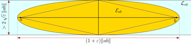
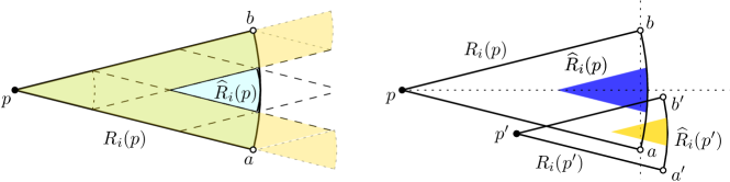
Let be finite. Every pair of points, , determines a (closed) line segment ; the relative interior of is denoted by . Let denote the ellipse with foci and , and great axis of weight , and let be the slab bounded by two lines parallel to and tangent to ; see Fig. 1. Note that the width of equals the minor axis of , which is . When , the vector is called primitive if and .
Consider the following two conditions for edges of a Euclidean -spanner for .
-
•
Empty ellipse condition: .
-
•
Empty slab condition: and all points in are on the line .
Observation 4.
Suppose is finite, is a -spanner for , and .
-
1.
If meets the empty ellipse condition, then .
-
2.
If is a section of , , and meets the empty slab condition, then .
Proof.
The ellipse contains all points satisfying . By the triangle inequality, every point along an -path of weight at most satisfies this inequality, hence the entire path lies in . The empty ellipse condition implies that such a path cannot have interior vertices.
If is the integer lattice, then implies that is a primitive vector, hence the distance between any two lattice points along the line is at least . Given that , the empty slab condition now implies the empty ellipse condition. ∎
2.1 Lower Bounds for the Grid
We can now establish the lower bound in Theorem 2.
Lemma 5.
For every and every integer , the weight of every -spanner for the section of the integer lattice is .
Proof.
Let and . Denote the origin by . For every grid point , we have . We show that every primitive vector with satisfies the empty slab condition. It is clear that . Let be a point that is not on the line spanned by . By Pick’s theorem, . Since , then the distance between the line spanned by and is at least ; and so , as claimed.
By elementary number theory, is primitive for points . Indeed, every is relatively prime to integers in every interval of length , where is Euler’s totient function, and . Consequently, the total weight of primitive vectors , , is .
The edges , for all primitive vectors with , form a star centered at the origin. The translates of this star to other points , with are also present in every -spanner for . As every edge is part of at most two such stars, summation over stars yields a lower bound of . ∎
Remark 6.
The lower bound in Lemma 5 derives from the total weight of primitive vectors with , which satisfy the empty slab condition. There are additional primitive vectors that satisfy the empty ellipse condition (e.g., with for all ). However, it is unclear how to account for all vectors satisfying the empty ellipse condition, and whether their overall weight would improve the lower bound in Lemma 5.
Remark 7.
The empty ellipse and empty slab conditions each imply that an edge must be present in every -spanner for . It is unclear how the total weight of such “must have” edges compare to the minimum weight of a -spanner.
Remark 8.
We obtain a grid of points in the unit square if we scale down the section of the integer lattice by a factor of . The EMST of this grid has weight . Le and Solomon [40] proved that the greedy -spanner has weight , although the true performance of the greedy algorithm might be better. In contrast, Theorem 1 yields a -spanner of weight ; and Corollary 3 further improves it to .
2.2 Lower Bounds in the Unit Square
We continue with the lower bound in Theorem 1.
Lemma 9.
For every and every integer , there exists a set of points in such that every -spanner for has weight .
Proof.
First let be a set of points, where , with equally spaced points on two opposite sides of a unit square. By the empty ellipse property, every -spanner for contains a complete bipartite graph . The weight of each edge of is between and , and so the weight of every -spanner for is .
For , consider an grid of unit squares, and insert a translated copy of in each unit square. Let be the union of these copies of ; and note that . A -spanner for each copy of still requires a complete bipartite graph of weight . Overall, the weight of every -spanner for is .
Finally, scale down by a factor of so that it fits in a unit square. The weight of every edge scales by the same factor, and the weight of a -spanner for the resulting points in is , as claimed. ∎
Remark 10.
The points in the lower bound construction above lie on axis-parallel lines in , and so the weight of their EMST is . Recall that the lightness of the greedy -spanner is [40]. For , it yields a -spanner of weight . Note that the greedy algorithm returns a -spanner of nearly minimum weight in this case.
3 Spanner Algorithm: Sparse Yao-Graphs
For clarity, we present our new spanner algorithm in full detail in the plane (in this section), and then sketch the straightforward generalization to (in Section 5). Let be a set of points in and . As noted above, the Yao-graph with cones per vertex is a -spanner for [6, 16]. We describe a new algorithm, SparseYao, by modifying the classical Yao-graph construction (Section 3.1); and show that it returns a -spanner for (Section 3.2). Later, we use this algorithm for points in the unit square (Section 4; and for an section of the integer lattice (Section 6).
The basic idea is that, in some cases, cones of aperture suffice for the inductive proof that establishes the spanning ratio . This idea is fleshed out in Section 3.2. The use of the angle then allows us to charge the weight of the resulting spanner to the area of empty regions (specifically, to an empty section of a cone) in Section 4.
3.1 Sparse Yao-Graph Algorithm
We present an algorithm that computes a modified version of the Yao-graph for a point set and parameter . It starts with cones of aperture , and refines them to cones of aperture . We connect each point to the closest point in each large cone, and add edges in the small cones only if necessary. To specify when exactly the small cones are needed, we define two geometric regions that will also play crucial roles in the stretch and weight analyses.
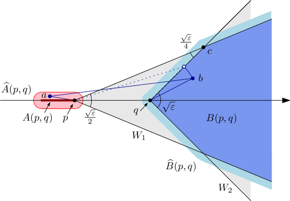
Definitions. Let be distinct points; refer to Fig. 2. Let be the line segment of weight on the line with one endpoint at but interior-disjoint from the ray ; and the set of points in within distance from . Let be the cone with apex , aperture , and symmetry axis ; and let be the cone with apex , aperture , and the same symmetry axis . Let . Finally, let be the set of points in within distance at most from .
We show below (Lemma 15) that if we add edge to the spanner, then we do not need any of the edges with and . We can now present our algorithm.
Algorithm SparseYao.
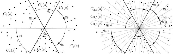
Input: a set of points, and .
Preprocessing Phase. Subdivide into congruent cones of aperture with apex at the origin, denoted . For , let be the symmetry axis of directed from the origin towards th interior of . For each , subdivide into congruent cones of aperture , denoted ; see Fig. 3. For each point , let and , resp., be the translates of cones and to apex .
For all and , let be a closest point to in , if such a point exists. For every and , let be the list of all ordered pairs with , sorted in decreasing order of the orthogonal projection of to (e.g., if is the -axis, then is sorted by decreasing -coordinates of the points .) For every , let be the concatenation of the lists by decreasing (i.e., shorter edges first).
For all , indices , and parameter , let denote a closest point to that lies in and satisfies ; if such a point exists.
Main Phase: Computing a Spanner. Initialize an empty graph with .
-
1.
For all , do:
-
•
While the list is nonempty, do:
-
(a)
Let be the first ordered pair in , and put for short.
-
(b)
Add (the unordered edge) to .
-
(c)
For all and , do:
Put . If , then add to . -
(d)
For every , including , delete the pair from .
-
(a)
-
•
-
2.
Return .
Remark 11.
Each is sorted by two criteria: the sublists are sorted by orthogonal projections of the apices to the directed lines , and itself sorted by weight rounded down to the nearest power of two. The order by weight is used in the stretch analysis, and the order by projections in the weight analysis.
The main algorithm adds edges to the graph in steps 1b and 1c in each while loop. In step 1b, it adds some of the edges of the Yao graph , where . It does not necessarily add all edges of : Initially all edges of are in the lists , but some of them may be removed from in a step 1d, and they may not be added to .
In step 1b, the algorithm adds edges from point to some points in the cones , where (i.e., small cones contained in three consecutive large cones). In the large cone , we know that is a closest point to , so for the points are the closest points to in the small cones. However, for , the points are not necessarily closest to in : they are the closest to among points at distance at least from . Furthermore, an edge is added to only if does not lie in the region shown in Fig. 2. This guarantees that is comparable to . The lower bound will be used in the stretch analysis, and the upper bound in the weight analysis.
Remark 12.
It is clear that the runtime of Algorithm SparseYao is polynomial in . In particular, the preprocessing phase constructs the Yao-graph with edges. A data structure that can return for a query could be based on standard range searching data structures [2]; or simply by sorting all edges by weight in each cone in time. The main phase of the algorithm computes the graph in time. Optimizing the runtime, however, is beyond the scope of this paper.
3.2 Stretch Analysis
In this section, we show that is a -spanner for . We know that the Yao-graph with cones is a -spanner for . The following seven lemmas justify that we do not need edges in all cones to obtain a -spanner.
The first three technical lemmas show that if already contains -paths from to and from to , then we can concatenate them with the edge to obtain a -path from to . We start with the special case that and in Lemma 13, then extend it to the case when and in Lemma 14. The general case, where and , is tackled in Lemma 15. In inequalities (3) and (4) below, we use and , resp., instead of to leave room to absorb further error terms in the general case.
Lemma 13.
Let . For any two points and , we have
| (3) |
Proof.
We start with two simplifying assumptions.
(i) We may assume that is the origin, is on the positive -axis, and is on or above the -axis, by applying a suitable congruence if necessary.
(ii) We may assume w.l.o.g. that is in the boundary of , since if we rotate the segment around , then the left hand side of (3) does not change, but the right hand side is minimized for .
Let us review the Taylor estimates of some of the trigonometric functions. For the secant function, we use the upper bound for . For the tangent function, we use the lower and upper bounds for .
To prove (3), we distinguish between two cases based on whether or . Let be the intersection point of and above the -axis. Since , then is an isosceles triangle with .
Case 1: (Fig. 4(left)).
Note that . Assume for some . Since the interior angles of triangle add up to , then .
Let be the orthogonal projection of to . Then . Since implies , then we have , and so .
Case 2: (Fig. 4(right)).
In this case, is fixed. Note that . Assume for some .
Since implies , then we get hence . Furthermore, the right triangles and yield
This further implies
For points , let be the line segment of weight on the line with one endpoint at but interior-disjoint from the ray . In particular, we have .
Lemma 14.
For all and , we have
| (4) |
Proof.
Note that implies since lies on the common symmetry axis of , , and . Then (3) can be written as
| (5) |
as for . ∎
In the general case, we have and . However, for technical reasons (cf. Lemma 18 below), we use a larger neighborhood instead of . Recall that is the set of points in within distance from . Now let be the set of points in within distance at most from .
Lemma 15.
For all and , we have
| (6) |
Proof.
Since and , then there exist and with and . In particular, . Combining these inequalities with Lemma 14 for points and , we obtain
for , as claimed. ∎
Relation between and .
The following two lemmas help analyze step 1c of Algorithm SparseYao that adds some of the edges to the spanner. For points , recall that , where and are wedges of aperture and , resp.; see Fig. 2.
Lemma 16.
Let , and . For every , we have .
Proof.
The line segment decomposes into two isosceles triangles. By the triangle inequality, the diameter of each isosceles triangle is less than . This implies that for any point , we have . ∎
The following lemma justifies the role of the regions in step 1d of the algorithm.
Lemma 17.
Let , and assume that for some indices and , where is a closest point to in at distance at least from . If but , then .
Proof.
Since and the aperture of each is , then , and so . Lemma 16 yields . Both and are in the cone . Consider the circle of radius centered at ; see Fig. 5. Since , and , , this circle intersects in the cone . Denote by the intersection point. Now implies that . The distance is bounded above by the length of the circular arc between them: . As , we have , and so , as required. ∎
We can also clarify the relation between and in the setting used in the stretch analysis. Specifically, we show for .
Lemma 18.
Let , and let be a closest point to in , and a closest point to among all points in at distance at least from , for some indices and . Then .
Proof.
By our assumptions, we have and . Since the aperture of each cone is , then . As , then
Consequently, every point in is within distance at most
from . By the triangle inequality, every point in the -neighborhood of is at distance at most from segment . ∎
Finally, we show that the cones , , and in step 1c of Algorithm SparseYao jointly cover any point if and ; see Fig. 6.
Lemma 19.
Let such that is the closest point to in the cone . Let and such that . Then
| (7) |
Proof.
Recall that the aperture of cone is . Assume w.l.o.g. that is the origin, and the symmetry axis of the cone is the is the positive -axis. Assume further that and in this coordinate system. It is enough to show that the angle between segment and the positive -axis is less than . In the remainder of the proof, we estimate the tangent of this angle.
Since and , the coordinates of vector are bounded by
Since and , then the coordinates of are bounded by
These bounds yield
Using the Taylor estimate in this range, the angle between segment and the positive -axis is less than . This completes the proof of (7). ∎
Completing the Stretch Analysis.
We are now ready to present the stretch analysis for SparseYao.
Theorem 20.
For every finite point set and , the graph is a -spanner.
Proof.
Let be a set of points in the plane. Let be the list of all edges of the complete graph on in increasing order by Euclidean weight (with ties broken arbitrarily). For , let be the -th edge in , and let . We prove the following by induction on :
Claim 21.
For every edge , contains an -path of weight at most .
For , the claim clearly holds, as the shortest edge is necessarily the closest points to in the cone , and so the algorithm adds to . Assume that and Claim 21 holds for . If the algorithm added edge to , then Claim 21 trivially holds for .
Suppose that . Let , and for some . Let and be points specified in the preprocessing phase of Algorithm SparseYao. We distinguish between two cases.
(1) The algorithm added the edge to . Note that and . By the induction hypothesis, contains a -path of weight at most and a -path of weight at most . If , then is a -path of weight at most by Lemma 15. Otherwise, . In this case, by Lemma 17. This means that the algorithm added the edge to . We have by Lemma 17, and so is a -path of weight at most by Lemma 15.
(2) The algorithm did not add the edge to . Then the algorithm deleted from the list in some step 1d; and in step 1b of the same iteration, it added another edge to , where is the closest point to in the cone chosen in the preprocessing phase of Algorithm SparseYao. This means that . Since is the concatenation of the lists according to increasing weight, then .
By Lemma 19 (with the roles of and interchanged), we have . We can now distinguish between two subcases:
(2a) . By induction, contains a -path of weight at most and a -path of weight at most . By Lemma 15 (with and ), the concatenation is a -path of weight at most .
(2b) . Then Lemma 19 implies for some and . We claim that . Indeed, we have by assumption. Since and , then . Now the triangle inequality yields .
Let be the closest point to in the cone at distance at least from , as specified in the preprocessing phase of Algorithm SparseYao. Since , then Lemma 17 gives . Thus the algorithm added the edge in step 1c. Since , then we have by Lemma 18; and by Lemma 17. By induction, contains a -path of weight at most , and a -path of weight at most . The concatenation is a -path of weight at most by Lemma 15.
4 Spanners in the Unit Square
In this section we show that, for a set of points and , Algorithm SparseYao returns a -spanner of weight (Theorem 29). Recall that for all and all , denotes a closest point to in the cone of aperture , if it exists, may or may not be an edge in . Let
We first show that the weight of the edges in approximates the weight of all other edges.
Lemma 22.
If Algorithm SparseYao adds and to in the same iteration, then .
Proof.
Lemma 23.
For , we have .
Proof.
Fix and . Put , for short, and suppose that . Consider the step of the algorithm that adds the edge to , together with up to edges of type , where and . By Lemma 22, . The total weight of all edges added to the spanner is
Summation over all edges in yields . ∎
It remains to show that . For , let
that is, the set of edges in between points and a closest point in cone of aperture at most . We prove that in Lemma 28 below. Since this will immediately imply .
Charging Scheme.
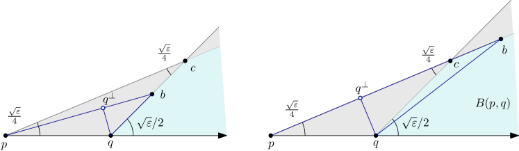
Let be fixed. Assume w.l.o.g. that the symmetry axis of the cone is horizontal, and the apex is the leftmost point in . Refer to Fig. 7(left). For each edge , let be the intersection of cone and the disk of radius centered at . Note that is a sector of the disk; and the sectors , for all , are pairwise homothetic. The sector has three vertices: Its leftmost vertex is , and the other two vertices are the endpoints of a circular arc, which have the same -coordinate (by symmetry). As is a closest point to in , then .
Let be the set of sectors for all edges in . These sectors are not necessarily disjoint; but we can still prove a lower bound on the area of their union. We first study their intersection pattern.
Lemma 24.
Assume that and . Then and have smaller -coordinates than any other vertices of the two sectors.
Proof.
Denote the vertices of and by and , resp.; see Fig. 7(right). Point is in the exterior of , since . Now implies that boundaries of and intersect.
Suppose, to the contrary, lies to the right of the vertical line . Since is the leftmost point of , then all intersection points in are on the circular arc . If or intersects the circular arc , then , a contradiction. Otherwise only the circular arcs and intersect: Then both and lie on the orthogonal bisector of the two intersection points; and we arrive again at a contradiction . ∎
We partition the sectors according to their diameters: For all , let be the set of sectors such that . We show that the sectors do not overlap too heavily.
Lemma 25.
For all , any point is contained in sectors in .
Proof.
Let be the set of sectors in that contain ; these sectors pairwise intersect. By Lemma 24, the leftmost vertices of the sectors have smaller -coordinates than any other vertices (i.e., endpoints of circular arcs). Let be a vertical line that separates the leftmost vertices of these sectors from all other vertices; and let be the left halfplane bounded by ; see Fig. 8(left).
Recall that for every sector , we have . As the aperture of is at most , with , then the weight of the vertical segment is at most .
For every sector , the region is an isosceles triangle with two legs of slopes . Consider the union of these isosceles triangles, . Its right boundary is of a vertical segment of weight along ; and its left boundary is a -monotone curve, that we denote by . All local -minima of are leftmost vertices of the sectors .
We claim that if are two consecutive local -minima along , then
| (8) |
that is the -coordinates of and differ by at least ; refer to Fig. 8(right). Suppose, to the contrary, that . Due to the slopes of , this implies
Assume w.l.o.g. that Algorithm SparseYao added edge to before . As the list is sorted by decreasing -coordinates, then . When the algorithm added edge to , it deleted all pairs from such that . Given that and , then is a line segment of weight and slope of absolute value at most . This implies that lies in the -projection of . Furthermore, the distance between and the point with the same -coordinate in is at most . Recall that contains every point in an -neighborhood of . Consequently, , and the algorithm deleted from when it added to . This contradicts the assumption , and proves the claim (8).
As the height of is . Combined with (8), this implies that has at most local -minima. Thus , as claimed. ∎
The sectors in are not necessarily disjoint. In order to obtain disjoint regions, we define the core of a sector , denoted ; see Fig. 9(left). Label the vertices of by , , and , where . Let be the vector along the angle bisector of of weight . Now denote the region obtained by scaling from center with ratio ; and let . By construction, we have and .
Lemma 26.
If , then any two sectors in and have disjoint cores.
Proof.
Let and with . Label their vertices by , , and , , , resp., in counterclockwise order; see Fig. 9(right). Note that
Suppose, for the sake of contradiction, that . Since and , then . By Lemma 24, lies to the left of the vertical line . Given that , the point cannot be in the interior of , that is, . The combination of these two observation yields .
We may assume that lies below the line by a reflection in the -axis, if necessary. Since the sector has a horizontal symmetry axis and , then lies below the line ; and the core lies below the line . Recall that the vectors and are parallel, and implies . Consequently, lies below the line . However, by construction, lies above the line . This implies that the cores and are disjoint. ∎
The combination of Lemmas 25 and 26 gives the following bound on the total area of all sectors of a given direction.
Lemma 27.
For every , we have .
Proof.
Lemma 28.
For every , we have .
Proof.
For every sector , we have
In particular, summation over all edges and Jensen’s inequality gives
where is the average weight of an edge in . Combined with Lemma 27, we obtain
| (9) | ||||
Finally, , as required. ∎
Theorem 29.
For every set of points in and every , Algorithm SparseYao returns a Euclidean -spanner of weight .
5 Generalization to Higher Dimensions
Upper Bound.
For every constant , Algorithm SparseYao and its analysis generalize to . We sketch the necessary adjustments for a point set . Recall that for , we partitioned the plane into cones , of aperture . In -dimensions, we can cover with cones of aperture such that every point in is covered by at most cones. With these cones, Algorithm SparseYao and its stretch analysis goes through almost verbatim. We point out a few dimension-dependent details: In step 1c of Algorithm SparseYao, instead of three consecutive cones , we need cones that cover a -neighborhood of , in spherical distance with respect to . For the stretch analysis, the key technical lemmas directly generalize to -space: In Lemmas 13—18, the points , , , and are coplanar in ; and in Lemma 15 and 18, the regions and are small neighborhoods of and , resp., independent of dimension.
For the weight analysis of the spanner also generalizes. Standard volume argument shows that every cone of aperture is covered by cones of aperture . Thus the direct generalization of Lemma 23 yields , where is partitioned into subsets .
In the generalization of Lemma 25, every generic point is contained in regions : In the proof, however, the -monotone curve is replaced by a -dimensional surface/terrain. In the weight analysis for , we need to charge the weight of each edge to an empty sector , which is the intersection of a cone of aperture and a ball of radius . The volume of such a region is . The core of the sectors can be defined analogously, and Lemmas 26–27 extend to -space. Finally, in the proof of Lemma 28, Jensen’s inequality is used for the function . In particular, for the average weight of an edge in , , inequality (9) becomes
| (10) | ||||
and . Overall,
Lower Bound.
The empty ellipse condition and the lower bound construction readily generalize to every dimension . Let be a set of points, where , with points arranged in a grid on two opposite faces of a unit cube . By the empty ellipsoid condition, every -spanner for contains a complete bipartite graph , of weight . if we arrange translated copies of in a grid, we obtain a set of points, and a lower bound of . Scaling by a factor of yields a set of points in for which any -spanner has weight .
6 Spanners for the Integer Lattice
We briefly review known results from analytic number theory in Section 6.1, and derive upper bounds on the minimum weight of a -spanner for the grid: First we analyze the weight of Yao-graphs (Section 6.2), and then refine the analysis for Sparse Yao-graphs in (Section 6.3).
6.1 Preliminaries: Farey Sequences
Two points in the integer lattice are visible if the line segment does not pass through any lattice point. An integer point is visible from the origin if and are relatively prime, that is, . The slope of a segment between and is . For every , the Farey set of order ,
is the set of slopes of the lines spanned by the origin and lattice points with . The Farey sequence is the sequence of elements in in increasing order. Note that . Farey sets and sequences have fascinating properties, and the distribution of , as is not fully understood. It is known that
where is Euler’s totient function (i.e., is the number of nonnegative integers with and ). Furthermore, if and are consecutive terms of the Farey sequence in reduced form (i.e., and ), then [34]. The Farey sequence is uniformly distributed on in the sense that for any fixed subinterval , the asymptotic frequency of the Farey set in is known converge as tends to infinity [21]:
The error term is bounded by , for some . However, determining the rate of convergence is known to be equivalent to the Riemann hypothesis [26, 38]; see also [42] and references therein.
The key result we use is a bound on the average distance to a Farey set . For every , let
denote the distance between and the Farey set . Kargaev and Zhigljavsky [35] proved that
| (11) |
6.2 The Weight of Yao-Graphs for the Grid
Lemma 30.
For a positive integer , consider the subdivision of the unit interval into subintervals, . For every , let be the smallest positive integer such that for some integer . Then
-
(i)
, and
-
(ii)
.
Proof.
Let be an interval of length . If contains a point , then . Otherwise, is disjoint from the Farey set , and then for all . In the latter case,
| (12) |
For every positive integer , let be the number of intervals in that are disjoint from . Note that for , since all (closed) intervals contain a rational of the form . In particular, we have for all .
The combination of (11) and (12) yields . If we set for a sufficiently large constant , then
That is, at most of intervals are disjoint from . For the remaining at least intervals, we have , and the sum of these terms is . It remains to bound the sum of terms in the intervals disjoint form . We use a standard diadic partition. Let . Then
The completes the proof of (i). It remains to prove (ii).
Recall that we set for a sufficiently large constant , then . That is, at most of intervals are disjoint from . For the remaining at least intervals, we have , and the sum of terms for these indices is . It remains to bound the sum of terms in the intervals disjoint form . Let . Then
as claimed. ∎
Lemma 31.
For a positive integer , consider the subdivision of the plane into cones, each with apex at the origin , and aperture . For each , let be a point in the th cone that lies closest to the origin. Then .
Proof.
The function is a monotone increasing bijection from the interval to . Its derivative is bounded by . Consequently, it distorts the length of any interval by a factor of at most 2. That is, it maps any interval to an interval with .
Recall that Algorithm SparseYao operates on cones . The two coordinate axes and the lines subdivide the plane into eight cones with aperture . These four lines contain a set of eight rays emanating from the origin. A cone that contains any ray in necessarily contains a lattice point with . Consider the cones between two consecutive rays in ; there are such cones. Rotate these cones by a multiple of so that they correspond to slopes in the interval . Due to the rotational symmetry of , the rotation is an isometry on . Each cone is an interval of angles with . As noted above, this corresponds to an interval of slopes with .
Subdivide the interval into subintervals of length . Each interval contains at least one intervals of this subdivision. Let be the smallest positive integer such that there exists a rational in the th interval. Then the lattice point lies in . Since , then , and so the distance between and the origin is at most . Let be a point in closest to the origin, hence . By Lemma 30(i), we conclude that , where the summation is over cones bounded by two consecutive rays in . Summation over all octants readily yields . ∎
Corollary 32.
For positive integers and , let be the Yao-graph with cones on the points in the section of the integer lattice. Then .
Proof.
Recall the Yao-graph is defined as a union of stars, one for each vertex. For each vertex , a star is obtained by subdividing the plane into cones with apex and aperture , and connecting to the closes point in the cone (if such a point exists). By Lemma 31, for any . Summation over vertices yields . ∎
For every finite point set , the Yao-graph with cones per vertex is a -spanner. Corollary 32 readily implies that the section of the integer lattice admits a -spanner of weight .
6.3 The Weight of Sparse Yao-Graphs for the Grid
Theorem 33.
Let be the section of the integer lattice for some positive integer . Then the graph SparseYao has weight .
Proof.
The edges in Algorithm SparseYao form a Yao-graph with cones per vertex. By Corollary 32, we have .
Algorithm SparseYao refines each cone of apex and aperture into cones , and adds some of the edges between and a closest point . It remains to bound the weight of the edges added to the spanner. Fix and . Suppose that the algorithm adds edges from to points of the form for and . We may assume w.l.o.g. that of these edges lie on the left side of the ray . Label these points in ccw order about as , and let . Then the triangles , for , are interior-disjoint, contained in , and spanned by lattice points in the . By Pick’s theorem, for all . Consequently, .
We also derive an upper bound on . Recall (cf. Fig. 2) that , where and are cones centered at and , with apertures and , respectively. Note that partitions into two congruent isosceles triangles, each with two sides of weight , and so . By contrasting the lower and upper bounds for , we obtain
By Lemma 22, if an edge was added in the same iteration as , then . Overall, the total weight of all edges added together with is . Summation over yields .
Using Lemma 30(ii) with , the total weight of the edges added for a vertex is . Summation over all vertices , gives an overall weight of , as claimed. ∎
The combination of Lemma 5 and Theorem 33 (lower and upper bounds) establishes Theorem 2. We restate Theorem 33 for points in the unit square .
Corollary 34.
Let be the section of the scaled lattice , contained in . Then has weight .
Proof.
Apply Theorem 33 for the section of the integer lattice , and then scale down all weights by a factor of . ∎
7 Conclusions
The SparseYao algorithm, introduced here, combines features of Yao-graphs and greedy spanners. It remains an open problem whether the celebrated greedy algorithm [6] always returns a -spanner of weight for points in the unit square (and for points in ). The analysis of the greedy algorithm is known to be notoriously difficult [25, 40]. It is also an open problem whether SparseYao or the greedy algorithm approximates the instance-minimal weight of a Euclidean -spanner within a ratio in , which would go below the best possible bound implied by lightness [40].
All results in this paper pertain to the Euclidean distance (i.e., -norm in ). Generalizations to -norms for (or Minkowski norms with respect to a centrally symmetric convex body in ) would be of interest. It is unclear whether some or all of the machinery developed here generalizes to other norms. Finally, we note that Steiner points can substantially improve the weight of a -spanner in Euclidean space [9, 40, 39]. It is left for future work to study the minimum weight of a Euclidean Steiner -spanner for points in the unit cube ; and for an section of the integer lattice .
The SparseYao algorithm is a modified version of the classical Yao-graph on a set of points in . It can easily be implemented in time by a brute-force algorithm after sorting the edges of the complete graph on points. Note, however, that Yao-graphs in the plane can be constructed in time [15, 27]; and -graphs in can be computed time [45]: These bounds are near-linear in for constant . It remains an open problem whether the algorithm SparseYao or its adaptation to -graphs can be implemented in near-linear time for constant and dimension . For a section of the integer lattice in the plane, the SparseYao algorithm can be implemented in time due to symmetry: One can find a closest lattice points to the origin in each cone in time, and then translate the resulting star to all other lattice points.
References
- [1] A. Karim Abu-Affash, Gali Bar-On, and Paz Carmi. -Greedy -spanner. Comput. Geom., 100:101807, 2022. doi:10.1016/j.comgeo.2021.101807.
- [2] Pankaj K. Agarwal. Range searching. In Jacob E. Goodman, Joseph O’Rourke, and Csaba D. Tóth, editors, Handbook of Discrete and Computational Geometry, chapter 40, pages 1057–1092. CRC Press, Boca Raton, FL, 3rd edition, 2017. doi:10.1201/9781315119601.
- [3] Pankaj K. Agarwal, Yusu Wang, and Peng Yin. Lower bound for sparse Euclidean spanners. In Proc. 16th ACM-SIAM Symposium on Discrete Algorithms (SODA), pages 670–671, 2005. URL: http://dl.acm.org/citation.cfm?id=1070432.1070525.
- [4] Oswin Aichholzer, Sang Won Bae, Luis Barba, Prosenjit Bose, Matias Korman, André van Renssen, Perouz Taslakian, and Sander Verdonschot. Theta-3 is connected. Comput. Geom., 47(9):910–917, 2014. doi:10.1016/j.comgeo.2014.05.001.
- [5] Hugo A. Akitaya, Ahmad Biniaz, and Prosenjit Bose. On the spanning and routing ratios of the directed -graph. Comput. Geom., 105-106:101881, 2022. doi:10.1016/j.comgeo.2022.101881.
- [6] Ingo Althöfer, Gautam Das, David P. Dobkin, Deborah Joseph, and José Soares. On sparse spanners of weighted graphs. Discret. Comput. Geom., 9:81–100, 1993. doi:10.1007/BF02189308.
- [7] Sunil Arya and Michiel H. M. Smid. Efficient construction of a bounded-degree spanner with low weight. Algorithmica, 17(1):33–54, 1997. doi:10.1007/BF02523237.
- [8] Luis Barba, Prosenjit Bose, Mirela Damian, Rolf Fagerberg, Wah Loon Keng, Joseph O’Rourke, André van Renssen, Perouz Taslakian, Sander Verdonschot, and Ge Xia. New and improved spanning ratios for Yao graphs. J. Comput. Geom., 6(2):19–53, 2015. doi:10.20382/jocg.v6i2a3.
- [9] Sujoy Bhore and Csaba D. Tóth. Euclidean steiner spanners: Light and sparse. SIAM J. Discret. Math., 36(3):2411–2444, 2022. URL: https://doi.org/10.1137/22m1502707, doi:10.1137/22M1502707.
- [10] Glencora Borradaile, Hung Le, and Christian Wulff-Nilsen. Greedy spanners are optimal in doubling metrics. In Proc. 30th ACM-SIAM Symposium on Discrete Algorithms (SODA), pages 2371–2379, 2019. doi:10.1137/1.9781611975482.145.
- [11] Prosenjit Bose, Jean-Lou De Carufel, Pat Morin, André van Renssen, and Sander Verdonschot. Towards tight bounds on theta-graphs: More is not always better. Theor. Comput. Sci., 616:70–93, 2016. doi:10.1016/j.tcs.2015.12.017.
- [12] Prosenjit Bose, Darryl Hill, and Aurélien Ooms. Improved bounds on the spanning ratio of the theta-5-graph. In Proc. 17th Symposium on Algorithms and Data Structures (WADS), volume 12808 of LNCS, pages 215–228. Springer, 2021. doi:10.1007/978-3-030-83508-8_16.
- [13] Kevin Buchin, Sariel Har-Peled, and Dániel Oláh. A spanner for the day after. Discret. Comput. Geom., 64(4):1167–1191, 2020. doi:10.1007/s00454-020-00228-6.
- [14] Timothy M. Chan, Sariel Har-Peled, and Mitchell Jones. On locality-sensitive orderings and their applications. SIAM J. Comput., 49(3):583–600, 2020. doi:10.1137/19M1246493.
- [15] Maw-Shang Chang, Nen-Fu Huang, and Chuan Yi Tang. An optimal algorithm for constructing oriented Voronoi diagrams and geographic neighborhood graphs. Inf. Process. Lett., 35(5):255–260, 1990. doi:10.1016/0020-0190(90)90054-2.
- [16] Kenneth L. Clarkson. Approximation algorithms for shortest path motion planning. In Proc. 19th ACM Symposium on Theory of Computing (SoCG), pages 56–65, 1987. doi:10.1145/28395.28402.
- [17] Gautam Das, Paul J. Heffernan, and Giri Narasimhan. Optimally sparse spanners in 3-dimensional Euclidean space. In Proc. 9th Symposium on Computational Geometry (SoCG), pages 53–62, 1993. doi:10.1145/160985.160998.
- [18] Gautam Das and Giri Narasimhan. A fast algorithm for constructing sparse euclidean spanners. Int. J. Comput. Geom. Appl., 7(4):297–315, 1997. doi:10.1142/S0218195997000193.
- [19] Gautam Das, Giri Narasimhan, and Jeffrey S. Salowe. A new way to weigh malnourished Euclidean graphs. In Proc. 6th ACM-SIAM Symposium on Discrete Algorithms (SODA), pages 215–222, 1995. URL: http://dl.acm.org/citation.cfm?id=313651.313697.
- [20] Yefim Dinitz, Michael Elkin, and Shay Solomon. Low-light trees, and tight lower bounds for Euclidean spanners. Discret. Comput. Geom., 43(4):736–783, 2010. doi:10.1007/s00454-009-9230-y.
- [21] Fraçois Dress. Discrépance des suites de Farey. J. Théor. Nombres Bordeaux, 11(2):345–367, 1999. URL: http://eudml.org/doc/248344.
- [22] Adrian Dumitrescu and Anirban Ghosh. Lattice spanners of low degree. Discret. Math. Algorithms Appl., 8(3):1650051:1–1650051:19, 2016. doi:10.1142/S1793830916500518.
- [23] Michael Elkin and Shay Solomon. Optimal Euclidean spanners: Really short, thin, and lanky. J. ACM, 62(5):35:1–35:45, 2015. doi:10.1145/2819008.
- [24] Leonard Few. The shortest path and the shortest road through points. Mathematika, 2(2):141–144, 1955. doi:10.1112/S0025579300000784.
- [25] Arnold Filtser and Shay Solomon. The greedy spanner is existentially optimal. SIAM J. Comput., 49(2):429–447, 2020. doi:10.1137/18M1210678.
- [26] Jérôme Franel. Les suites de Farey et les problèmes des nombres premiers. Nachrichten von der Gesellschaft der Wissenschaften zu Göttingen, Mathematisch-Physikalische Klasse, pages 198–201, 1924. URL: http://eudml.org/doc/59156.
- [27] Daniel Funke and Peter Sanders. Efficient Yao graph construction. In Proc. 21st Symposium on Experimental Algorithms (SEA), volume 265 of LIPIcs, pages 20:1–20:20. Schloss Dagstuhl, 2023. doi:10.4230/LIPICS.SEA.2023.20.
- [28] Damien Galant and Cédric Pilatte. A note on optimal degree-three spanners of the square lattice. Discret. Math. Algorithms Appl., 14(3):2150124:1–2150124:12, 2022. doi:10.1142/S179383092150124X.
- [29] Jie Gao, Leonidas J. Guibas, and An Nguyen. Deformable spanners and applications. Comput. Geom., 35(1-2):2–19, 2006. doi:10.1016/j.comgeo.2005.10.001.
- [30] Lee-Ad Gottlieb. A light metric spanner. In Proc. 56th IEEE Symposium on Foundations of Computer Science (FOCS), pages 759–772, 2015. doi:10.1109/FOCS.2015.52.
- [31] Joachim Gudmundsson and Christian Knauer. Dilation and detours in geometric networks. In Handbook of Approximation Algorithms and Metaheuristics, volume 2. Chapman and Hall/CRC, 2nd edition, 2018.
- [32] Joachim Gudmundsson, Christos Levcopoulos, and Giri Narasimhan. Fast greedy algorithms for constructing sparse geometric spanners. SIAM J. Comput., 31(5):1479–1500, 2002. doi:10.1137/S0097539700382947.
- [33] Sariel Har-Peled. Geometric Approximation Algorithms, volume 173 of Mathematics Surveys and Monographs. AMS, 2011. doi:http://dx.doi.org/10.1090/surv/173.
- [34] Godfrey H. Hardy and Edward M. Wright. Farey series and a theorem of Minkowski. In An Introduction to the Theory of Numbers, chapter 3, pages 23–37. Clarendon Press, Oxford, 1979. doi:10.2307/3610026.
- [35] Pavel Kargaev and Anatoly Zhigljavsky. Approximation of real numbers by rationals: Some metric theorems. Journal of Number Theory, 61:209–225, 1996. doi:10.1006/jnth.1996.0145.
- [36] J. Mark Keil. Approximating the complete Euclidean graph. In Proc. 1st Scandinavian Workshop on Algorithm Theory (SWAT), volume 318 of LNCS, pages 208–213. Springer, 1988. doi:10.1007/3-540-19487-8_23.
- [37] J. Mark Keil and Carl A. Gutwin. Classes of graphs which approximate the complete Euclidean graph. Discret. Comput. Geom., 7:13–28, 1992. doi:10.1007/BF02187821.
- [38] Edmund Landau. Bemerkungen zu der vorstehenden Abhandlung von Herrn Franel. Göttinger Nachrichten, pages 202–206, 1924. Coll. works, vol. 8 (Thales Verlag, Essen).
- [39] Hung Le and Shay Solomon. Light Euclidean spanners with Steiner points. In Proc. 28th European Symposium on Algorithms (ESA), volume 173 of LIPIcs, pages 67:1–67:22. Schloss Dagstuhl, 2020. doi:10.4230/LIPIcs.ESA.2020.67.
- [40] Hung Le and Shay Solomon. Truly optimal Euclidean spanners. SIAM J. Computing, pages FOCS19–135–FOCS19–199, 2022. to appear. doi:10.1137/20M1317906.
- [41] Hung Le and Shay Solomon. A unified framework for light spanners. In Proc. 55th ACM Symposium on Theory of Computing (STOC), pages 295–308, 2023. doi:10.1145/3564246.3585185.
- [42] Andrew H. Ledoan. The discrepancy of Farey series. Acta Mathematica Hungarica, 156:465–480, 2018. doi:10.1007/s10474-018-0868-x.
- [43] Christos Levcopoulos, Giri Narasimhan, and Michiel H. M. Smid. Improved algorithms for constructing fault-tolerant spanners. Algorithmica, 32(1):144–156, 2002. doi:10.1007/s00453-001-0075-x.
- [44] Joseph S. B. Mitchell and Wolfgang Mulzer. Proximity algorithms. In Handbook of Discrete and Computational Geometry. CRC Press, Boca Raton, FL, 3rd edition, 2018.
- [45] Giri Narasimhan and Michiel H. M. Smid. Geometric Spanner Networks. Cambridge University Press, 2007. doi:10.1017/CBO9780511546884.
- [46] Satish Rao and Warren D. Smith. Approximating geometrical graphs via ”spanners” and ”banyans”. In Proc. 30th ACM Symposium on the Theory of Computing (STOC), pages 540–550, 1998. doi:10.1145/276698.276868.
- [47] Liam Roditty. Fully dynamic geometric spanners. Algorithmica, 62(3-4):1073–1087, 2012. doi:10.1007/s00453-011-9504-7.
- [48] Jim Ruppert and Raimund Seidel. Approximating the -dimensional complete Euclidean graph. In Proc. 3rd Canadian Conference on Computational Geometry (CCCG), pages 207–210, 1991. URL: https://cccg.ca/proceedings/1991/paper50.pdf.
- [49] Shay Solomon and Michael Elkin. Balancing degree, diameter, and weight in euclidean spanners. SIAM J. Discret. Math., 28(3):1173–1198, 2014. doi:10.1137/120901295.
- [50] J. Michael Steele and Timothy Law Snyder. Worst-case growth rates of some classical problems of combinatorial optimization. SIAM J. Comput., 18(2):278–287, 1989. doi:10.1137/0218019.
- [51] Kenneth J. Supowit, Edward M. Reingold, and David A. Plaisted. The travelling salesman problem and minimum matching in the unit square. SIAM J. Comput., 12(1):144–156, 1983. doi:10.1137/0212009.
- [52] Andrew Chi-Chih Yao. On constructing minimum spanning trees in -dimensional spaces and related problems. SIAM J. Comput., 11(4):721–736, 1982. doi:10.1137/0211059.