Configurational density of states and melting of simple solids

Abstract

We analyze the behavior of the microcanonical and canonical caloric curves for a piecewise model of the configurational density of states of simple solids, in the context of melting from the superheated state, as realized numerically in the Z-method via atomistic molecular dynamics. A first-order phase transition with metastable regions is reproduced by the model, being therefore useful to describe aspects of the melting transition. Within this model, transcendental equations connecting the superheating limit, the melting point, and the specific heat of each phase are presented and numerically solved. Our results suggest that the essential elements of the microcanonical Z curves can be extracted from simple modeling of the configurational density of states.

1 Introduction

One of the widely used approaches to determine the melting point of materials via atomistic computer simulation is the so-called Z-method [1, 2, 3, 4, 5, 6, 7, 8, 9, 10, 11], which is based on the empirical observation that the superheated solid at the limit of superheating temperature $T_{LS}$ has the same internal energy as the liquid at the melting temperature $T_{m}$. This observation has potential implications for understanding the atomistic melting mechanism from the superheated state [12, 13] but has been left mostly unexplored, disconnected from thermodynamical models of solids.

In the Z-method, the isochoric curve $T(E)$ is computed from simulations at different total energies $E_{1},E_{2},\ldots$ and the minimum temperature of the liquid branch of this isochoric curve is identified with the melting temperature $T_{m}$. This key assumption still lacks a proper explanation in terms of microcanonical thermodynamics of finite systems.

In this work, we study the properties of a recently proposed model [14] for the configurational density of states (CDOS) of systems with piecewise constant heat capacity by calculating its canonical and microcanonical caloric curves in terms of special functions. The model presents a first-order phase transition with metastable regions where the microcanonical curve $T(E)$ shows a so-called van der Waals loop [15]. The inflection points found in this loop can be associated to $T_{LS}$ and $T_{m}$ of the Z-method description of the superheated solid.

This paper is organized as follows. In Section 2 we briefly review the definition of the CDOS and the formalism used to compute thermodynamic properties from it. In Section 3 we revisit the model in Ref. [14] and provide some interpretation of its parameters. Sections  4 and  5 show the computation of the caloric curves of the solid model in the canonical and microcanonical ensemble, respectively, and we present some concluding remarks in Section  6.

2 Configurational density of states and thermodynamics

For a classical system with Hamiltonian

$$H(\bm{r}_{1},\ldots,\bm{r}_{N},\bm{p}_{1},\ldots,\bm{p}_{N})=\sum_{i=1}^{N}\frac{{\bm{p}_{i}}^{2}}{2m_{i}}+\Phi(\bm{r}_{1},\ldots,\bm{r}_{N}),$$ (1)

we will define the configurational density of states (CDOS) as the multidimensional integral

$$\mathcal{D}(\phi)\mathrel{\mathop{:}}=\int d\bm{r}_{1}\ldots d\bm{r}_{N}\>\delta(\Phi(\bm{r}_{1},\ldots,\bm{r}_{N})-\phi),$$ (2)

where $\Phi(\bm{r}_{1},\ldots,\bm{r}_{N})$ is the potential energy describing the interaction between particles. Using the definition of $\mathcal{D}(\phi)$ in (2) is possible to rewrite any configurational integral of the form

$$I=\int d\bm{r}_{1}\ldots d\bm{r}_{N}\>G(\Phi(\bm{r}_{1},\ldots,\bm{r}_{N}))$$ (3)

as a one-dimensional integral over $\phi$. In fact, taking $I$ and introducing a factor of 1 as an integral over a Dirac delta function, we have

$$\begin{split}I&=\int d\bm{r}_{1}\ldots d\bm{r}_{N}\>G(\Phi(\bm{r}_{1},\ldots,\bm{r}_{N}))\\ &=\int d\bm{r}_{1}\ldots d\bm{r}_{N}\left[\int_{-\infty}^{\infty}d\phi\delta(\phi-\Phi(\bm{r}_{1},\ldots,\bm{r}_{N}))\right]\>G(\Phi(\bm{r}_{1},\ldots,\bm{r}_{N}))\\ &=\int_{0}^{\infty}d\phi\left\{\int d\bm{r}_{1}\ldots d\bm{r}_{N}\delta(\phi-\Phi(\bm{r}_{1},\ldots,\bm{r}_{N}))\right\}\>G(\phi)\\ &=\int_{0}^{\infty}d\phi\mathcal{D}(\phi)G(\phi).\end{split}$$ (4)

where we have assumed that $\Phi$ has its global minimum at $\Phi=0$. One such integral of particular importance is the canonical partition function $Z(\beta)$, defined as

$$Z(\beta)\mathrel{\mathop{:}}=\int d\bm{\Gamma}\exp\big{(}-\beta H(\bm{\Gamma})\big{)},$$ (5)

where $\bm{\Gamma}=(\bm{r}_{1},\ldots,\bm{r}_{N},\bm{p}_{1},\ldots,\bm{p}_{N})$, and which can be computed, following (4), as

$$\begin{split}Z(\beta)=&\int d\bm{p}_{1}\ldots d\bm{p}_{N}\exp\Big{(}-\beta\textstyle\sum_{i=1}^{N}\frac{\bm{p}^{2}_{i}}{2m_{i}}\Big{)}\times\int d\bm{r}_{1}\ldots d\bm{r}_{N}\>\exp\Big{(}-\beta\Phi(\bm{r}_{1},\ldots,\bm{r}_{N})\Big{)}\\ =&\>Z_{0}(N)\>\beta^{-3N/2}\int_{0}^{\infty}d\phi\mathcal{D}(\phi)\exp(-\beta\phi)\\ =&\>Z_{0}(N)\>\beta^{-3N/2}Z_{c}(\beta),\end{split}$$ (6)

with $Z_{0}(N)\mathrel{\mathop{:}}=\prod_{i=1}^{N}(\sqrt{2\pi m_{i}})^{3}$ a constant only dependent on $N$ and the masses of the particles, and where

$$Z_{c}(\beta)\mathrel{\mathop{:}}=\int_{0}^{\infty}d\phi\mathcal{D}(\phi)\exp(-\beta\phi)$$ (7)

is the configurational partition function. Similarly, the full density of states,

$$\Omega(E)\mathrel{\mathop{:}}=\int d\bm{\Gamma}\delta(E-H(\bm{\Gamma}))$$ (8)

can also be computed from the CDOS, by a convolution with the density of states $\Omega_{K}$ of the ideal gas [16], that is,

$$\Omega(E)=\int d\phi\mathcal{D}(\phi)\Omega_{K}(E-\phi),$$ (9)

where

$$\Omega_{K}(E)\mathrel{\mathop{:}}=\int d\bm{p}_{1}\ldots d\bm{p}_{N}\delta\Big{(}\textstyle\sum_{i=1}^{N}\frac{\bm{p}^{2}_{i}}{2m_{i}}-E\Big{)}=\Omega_{0}(N)\Theta(E)E^{\frac{3N}{2}-1}.$$ (10)

In order to obtain the result in (9), we replace the integral over the momenta in $\Omega(E)$ by using (10),

$$\begin{split}\Omega(E)\mathrel{\mathop{:}}=&\int d\bm{r}_{1}\ldots d\bm{r}_{N}\>\left[\int d\bm{p}_{1}\ldots d\bm{p}_{N}\>\delta\Big{(}\textstyle\sum_{i=1}^{N}\frac{\bm{p}^{2}_{i}}{2m_{i}}+\Phi(\bm{r}_{1},\ldots,\bm{r}_{N})-E\Big{)}\right]\\ =&\int d\bm{r}_{1}\ldots d\bm{r}_{N}\>\Omega_{K}(E-\Phi(\bm{r}_{1},\ldots,\bm{r}_{N}))\\ =&\int_{0}^{\infty}d\phi\mathcal{D}(\phi)\Omega_{K}(E-\phi),\end{split}$$ (11)

where in the last equality we have used (4). Finally we have

$$\Omega(E)=\Omega_{0}(N)\int_{0}^{E}d\phi\mathcal{D}(\phi)(E-\phi)^{\frac{3N}{2}-1}=\Omega_{0}(N)\eta(E)$$ (12)

where $\Omega_{0}(N)\mathrel{\mathop{:}}=Z_{0}(N)/\Gamma\big{(}3N/2\big{)}$ is a function only of the size $N$ of the system, and

$$\eta(E)\mathrel{\mathop{:}}=\int_{0}^{E}d\phi\mathcal{D}(\phi)\big{(}E-\phi\big{)}^{\frac{3N}{2}-1}.$$ (13)

Now we have all the elements needed for the computation of the caloric curves and the transition energy (or temperature) for a given model of CDOS. In the canonical ensemble, the probability of observing a value $\phi$ of potential energy at inverse temperature $\beta$ is given by

$$P(\phi|\beta)=\frac{1}{Z_{c}(\beta)}\exp(-\beta\phi)\mathcal{D}(\phi)$$ (14)

and, using this, we can determine the caloric curve (internal energy as a function of inverse temperature) as

$$\big{<}H\big{>}_{\beta}=-\frac{\partial}{\partial\beta}\ln Z(\beta)=\frac{3N}{2\beta}+\big{<}\phi\big{>}_{\beta},$$ (15)

where

$$\big{<}\phi\big{>}_{\beta}=\frac{1}{Z_{c}(\beta)}\int_{0}^{\infty}d\phi\mathcal{D}(\phi)\exp(-\beta\phi)\phi=-\frac{\partial}{\partial\beta}\ln Z_{c}(\beta).$$ (16)

On the other hand, in the microcanonical ensemble the probability of having potential energy $\phi$ at total energy $E$ is given by [17, 18, 19, 20]

$$P(\phi|E)=\frac{1}{\eta(E)}(E-\phi)^{\frac{3N}{2}-1}\mathcal{D}(\phi).$$ (17)

The microcanonical caloric curve (inverse temperature as a function of internal energy) is given by

$$\beta(E)\mathrel{\mathop{:}}=\frac{\partial}{\partial E}\ln\Omega(E),$$ (18)

which can also be rewritten as an expectation as follows. Replacing $\Omega(E)$ in terms of $\eta(E)$ in (18) and using (17), we can write

$$\begin{split}\beta(E)&=\frac{1}{\eta(E)}\frac{\partial}{\partial E}\int_{0}^{E}d\phi\mathcal{D}(\phi)(E-\phi)^{\frac{3N}{2}-1}\\ &=\frac{1}{\eta(E)}\int_{0}^{E}d\phi\mathcal{D}(\phi)\big{(}E-\phi)^{\frac{3N}{2}-1}\left[\frac{3N-2}{2(E-\phi)}\right]=\big{<}\hat{\beta}_{K}\big{>}_{E}.\end{split}$$ (19)

where $\hat{\beta}_{K}$ is the kinetic inverse temperature estimator

$$\hat{\beta}_{K}(\phi;E)\mathrel{\mathop{:}}=\frac{3N-2}{2(E-\phi)}.$$ (20)

3 Model for the CDOS

In the following sections we will use, for the configurational density of states, the model presented in Ref. [14] which is defined piecewise, as

$$\mathcal{D}(\phi)=\begin{cases}d_{S}(\phi-\phi_{S})^{\alpha_{S}}\qquad\text{for}\;\phi<\phi_{c},\\[15.0pt] d_{L}(\phi-\phi_{L})^{\alpha_{L}}\qquad\text{for}\;\phi\geq\phi_{c}.\end{cases}$$ (21)

This model represents two segments, one for the solid phase which, by definition, will have potential energies $\phi<\phi_{c}$, and one for the liquid phase where $\phi\geq\phi_{c}$. That is, our main assumption is that the potential energy landscape is effectively divided into solid and liquid states by a surface

$$\Phi(\bm{r}_{1},\ldots,\bm{r}_{N})=\phi_{c}$$

in configurational space. By imposing continuity of the CDOS at $\phi=\phi_{c}$, we must have

$$d_{S}(\phi_{c}-\phi_{S})^{\alpha_{S}}=d_{L}(\phi_{c}-\phi_{L})^{\alpha_{L}}.$$ (22)

Here $\phi_{S}$ represents the potential energy minimum of the ideal solid, that can be set to zero without loss of generality provided that all energies are measured with respect to this value. We can also set $d_{S}$=1 and express the potential energy in units of $\phi_{c}$, and then we have

$$\mathcal{D}(\phi)=\begin{cases}\phi^{\alpha_{S}}\qquad\text{for}\;\phi<1,\\[15.0pt] \displaystyle\Big{(}\frac{\phi-\gamma}{1-\gamma}\Big{)}^{\alpha_{L}}\qquad\text{for}\;\phi\geq 1,\end{cases}$$ (23)

where we have defined the dimensionless parameter

$$\gamma\mathrel{\mathop{:}}=\frac{\phi_{L}}{\phi_{c}}.$$

In this way, the model for the CDOS has only three free parameters, namely $\alpha_{S}$, $\alpha_{L}$ and $\gamma$.

4 The caloric curve in the canonical ensemble

The configurational partition function $Z_{c}(\beta)$ associated to the model for the CDOS in (23) can be obtained by piecewise integration as

$$\begin{split}Z_{c}(\beta)&=\int_{0}^{\infty}d\phi\mathcal{D}(\phi)\exp(-\beta\phi)\\ &=\int_{0}^{1}d\phi\phi^{\alpha_{S}}\exp(-\beta\phi)+\frac{1}{(1-\gamma)^{\alpha_{L}}}\int_{1}^{\infty}d\phi(\phi-\gamma)^{\alpha_{L}}\exp(-\beta\phi)\\ &=\beta^{-(\alpha_{S}+1)}\int_{0}^{\beta}duu^{\alpha_{S}}\exp(-u)+\frac{\beta^{-(\alpha_{L}+1)}}{(1-\gamma)^{\alpha_{L}}}\int_{\beta}^{\infty}du(u-\beta\gamma)^{\alpha_{L}}\exp(-u)\\ &=\beta^{-(\alpha_{S}+1)}\int_{0}^{\beta}duu^{\alpha_{S}}\exp(-u)+\frac{\beta^{-(\alpha_{L}+1)}}{(1-\gamma)^{\alpha_{L}}}\exp(-\beta\gamma)\int_{\beta(1-\gamma)}^{\infty}dww^{\alpha_{L}}\exp(-w).\end{split}$$ (24)

Finally we obtain

$$Z_{c}(\beta)=\beta^{-(\alpha_{S}+1)}G_{S}(0\rightarrow\beta)+\frac{\beta^{-(\alpha_{L}+1)}}{(1-\gamma)^{\alpha_{L}}}\exp(-\beta\gamma)G_{L}(\beta(1-\gamma)\rightarrow\infty)$$ (25)

where we have defined, for convenience, the auxiliary functions

$$G_{\nu}(a\rightarrow b)\mathrel{\mathop{:}}=\int_{a}^{b}dt\exp(-t)t^{\alpha_{\nu}}=\Gamma(\alpha_{\nu}+1;b)-\Gamma(\alpha_{\nu}+1;a)$$ (26)

for $\nu=S,L$, where $\Gamma(k;x)\mathrel{\mathop{:}}=\int_{0}^{x}dt\exp(-t)t^{k-1}$ is the lower incomplete Gamma function.

4.1 Low and high-temperature limits

By taking the limit $\beta\rightarrow\infty$ of (25) we see that the second term vanishes, and also $G_{S}(0\rightarrow\infty)=\Gamma(\alpha_{S}+1)$ so for low temperatures we can approximate

$$Z_{c}(\beta)\approx\beta^{-(\alpha_{S}+1)}\Gamma(\alpha_{S}+1).$$ (27)

By replacing (27) in (16) we have

$$\big{<}\phi\big{>}_{\beta}=-\frac{\partial}{\partial\beta}\ln Z_{c}(\beta)\approx\frac{\alpha_{S}+1}{\beta}$$ (28)

and then the solid branch of the canonical caloric curve is given by a straight line,

$$E_{S}(T)\mathrel{\mathop{:}}=\big{<}H\big{>}_{T,S}=\frac{3N}{2}k_{B}T+\big{<}\Phi\big{>}_{T}=\big{(}\textstyle{\frac{3N}{2}}+\alpha_{S}+1\big{)}k_{B}T$$ (29)

as expected. Here we can verify that $E_{S}(T)\rightarrow 0$ as $T\rightarrow 0$, because we have fixed $\phi_{S}=0$, and moreover, we learn that the value of the specific heat for the solid phase is

$$C_{S}=\frac{d}{dT}E_{S}(T)=\big{(}\textstyle{\frac{3N}{2}}+\alpha_{S}+1\big{)}k_{B}.$$ (30)

On the other hand, for high temperatures (i.e. in the limit $\beta\rightarrow 0$) we can approximate

$$Z_{c}(\beta)\approx\left[\frac{\beta^{-(\alpha_{L}+1)}\exp(-\beta\gamma)}{(1-\gamma)^{\alpha_{L}}}\right]\Gamma(\alpha_{L}+1),$$ (31)

obtaining from (16) that

$$\big{<}\phi\big{>}_{\beta}=-\frac{\partial}{\partial\beta}\ln Z_{c}(\beta)\approx\frac{\alpha_{L}+1}{\beta}+\gamma$$ (32)

hence the liquid branch is also a straight line, given by

$$E_{L}(T)\mathrel{\mathop{:}}=\big{<}H\big{>}_{T,L}=\frac{3N}{2}k_{B}T+\big{<}\Phi\big{>}_{T}\approx\gamma+\big{(}\textstyle{\frac{3N}{2}}+\alpha_{L}+1\big{)}k_{B}T.$$ (33)

This allows us to interpret $\gamma$ as the extrapolation of the liquid branch towards $T=0$, that is, $\phi_{L}$ in units of $\phi_{c}$ is the potential energy of a perfectly frozen liquid at $T=0$,

$$E_{L}(T=0)=\gamma=\frac{\phi_{L}}{\phi_{c}}.$$ (34)

Moreover, we obtain that the specific heat of the liquid phase is

$$C_{L}=\frac{d}{dT}E_{L}(T)=\big{(}\textstyle{\frac{3N}{2}}+\alpha_{L}+1\big{)}k_{B}.$$ (35)

In order for the energy to be extensive in both branches as $N\rightarrow\infty$, it must hold true that the parameters $\alpha_{\nu}$ are proportional to $N$, and it follows that

$$\frac{C_{\nu}}{k_{B}}=\alpha_{\nu}+\frac{3N}{2}$$ (36)

with $\nu=S,L$. Using these definitions we can write $E_{S}$ and $E_{L}$ in terms of $\beta$ more compactly, as

$$E_{S}(\beta) =\frac{C_{S}}{\beta},$$ (37a)

$$E_{L}(\beta) =\gamma+\frac{C_{L}}{\beta}.$$ (37b)

4.2 Melting temperature

On account of the assumption that all solid states have $\phi<\phi_{c}$ and for the liquid states $\phi>\phi_{c}$, we will define the probabilities $P(S|\beta)$ of being in the solid phase, and $P(L|\beta)$ of being in the liquid phase as

$$P(S|\beta)\mathrel{\mathop{:}}=P(\phi<1|\beta) =\frac{1}{Z_{c}(\beta)}\int_{0}^{1}d\phi\exp(-\beta\phi)\phi^{\alpha_{S}}=\frac{\beta^{-(\alpha_{S}+1)}G_{S}(0\rightarrow\beta)}{Z_{c}(\beta)},$$ (38)

$$P(L|\beta)\mathrel{\mathop{:}}=P(\phi\geq 1|\beta) =\frac{1}{Z_{c}(\beta)}\int_{1}^{\infty}d\phi\exp(-\beta\phi)\frac{(\phi-\gamma)^{\alpha_{L}}}{(1-\gamma)^{\alpha_{L}}}=\frac{\beta^{-(\alpha_{L}+1)}\exp(-\beta\gamma)}{Z_{c}(\beta)(1-\gamma)^{\alpha_{L}}}G_{L}(\beta(1-\gamma)\rightarrow\infty)$$ (39)

respectively, such that

$$P(S|\beta)+P(L|\beta)=1$$

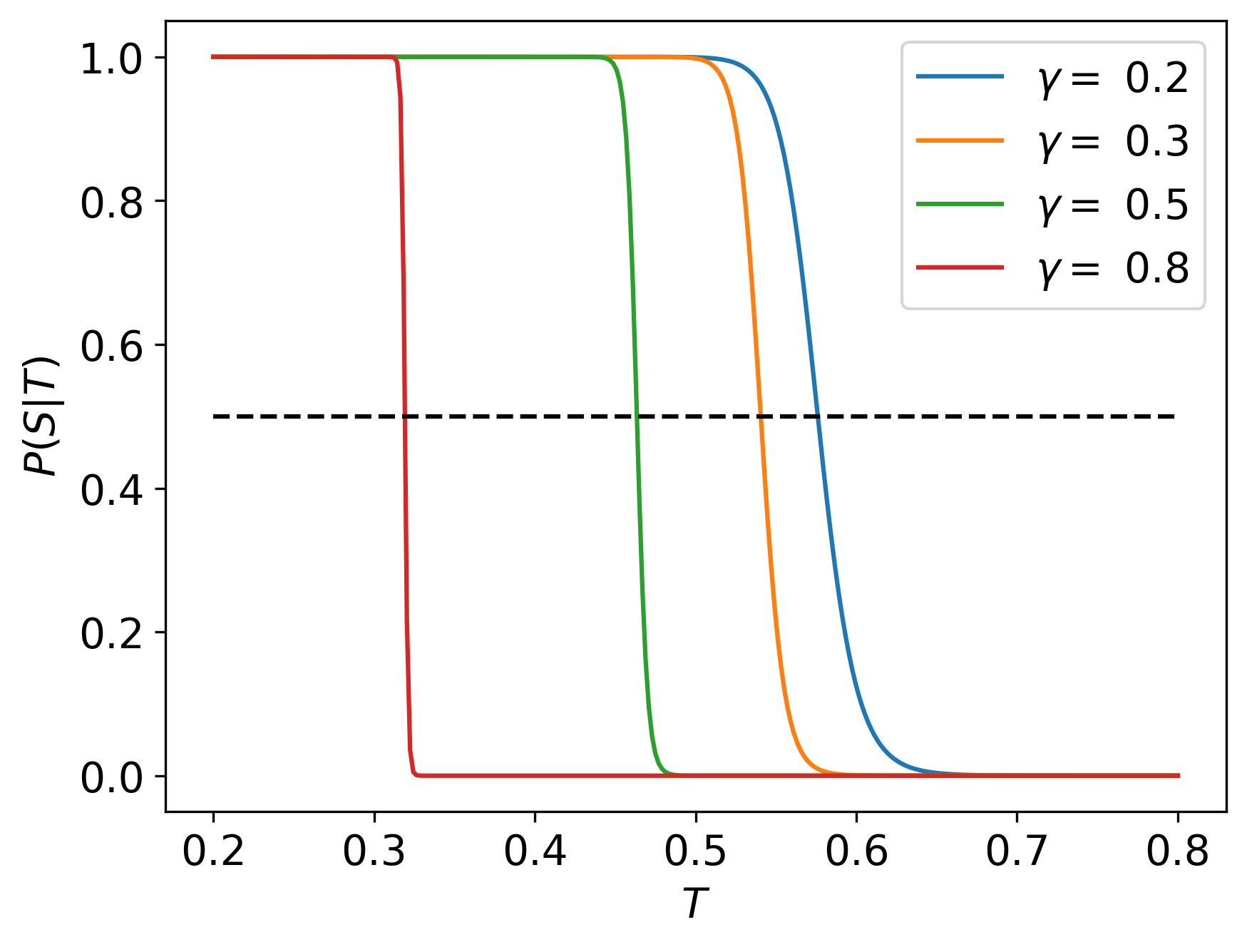
Figure 1: Canonical probability of solid phase $P(S|T)$ as a function of temperature, for different values of $\gamma$.

for all values of $\beta$. The probability of solid is shown as a function of $T$ in Fig. 1. The melting temperature $T_{m}$ is such that both probabilities are equal [21], that is,

$$P(S|\beta_{m})=P(L|\beta_{m})=\frac{1}{2},$$ (40)

with $\beta_{m}=1/(k_{B}T_{m})$, which is then the solution of the transcendental equation

$$(\beta_{m})^{\alpha_{L}-\alpha_{S}}G_{S}(0\rightarrow\beta_{m})=\frac{\exp(-\beta_{m}\gamma)}{(1-\gamma)^{\alpha_{L}}}G_{L}(\beta_{m}(1-\gamma)\rightarrow\infty).$$ (41)

Using $P(S|\beta)$ and $P(L|\beta)$ we can write the canonical caloric curve for any $\beta$ as the sum of three contributions, namely

$$\big{<}H\big{>}_{\beta}=\frac{3N}{2\beta}-\frac{\partial}{\partial\beta}\ln Z_{c}(\beta)=E_{S}(\beta)P(S|\beta)+E_{L}(\beta)\big{(}1-P(S|\beta)\big{)}+E_{\text{res}}(\beta),$$ (42)

where the first and second terms account for the solid and liquid branches, respectively, and $E_{\text{res}}$ is equal to

$$E_{\text{res}}(\beta)\mathrel{\mathop{:}}=-\frac{\gamma\beta^{-1}\exp(-\beta)}{Z_{c}(\beta)}.$$ (43)

By comparing (42) with the low and high temperature limits, namely $E_{S}$ and $E_{L}$, and noting that $P(S|\beta)\rightarrow 1$ for low temperatures and $P(S|\beta)\rightarrow 0$ for high temperatures, we see that $E_{\text{res}}$ must vanish on both limits, as can be verified by using (27) and (31). Therefore, this term is only relevant near the transition region. If we replace (41) into the configurational partition function in (25) we obtain

$$Z_{c}(\beta_{m})=2(\beta_{m})^{-(\alpha_{S}+1)}G_{S}(0\rightarrow\beta_{m})$$ (44)

and we can determine the melting energy $E^{*}$ as

$$E^{*}=\frac{3N}{2\beta_{m}}+\frac{1}{2}\left[N\gamma+\frac{\alpha_{S}+\alpha_{L}+2}{\beta_{m}}\right]-\frac{\gamma\exp(-\beta_{m})}{2G_{S}(0\rightarrow\beta_{m})}(\beta_{m})^{\alpha_{S}}.$$ (45)

Because $\alpha_{S}\propto N$, in the thermodynamic limit we can approximate

$$\begin{split}G_{S}(0\rightarrow\beta_{m})&=\int_{0}^{\beta_{m}}dt\exp(-t)t^{\alpha_{S}}\\ &=\int_{0}^{\beta_{m}}dt\exp(-t+\alpha_{S}\ln t)\\ &\approx\int_{0}^{\beta_{m}}dt\exp(\alpha_{S}\ln t)=\frac{\beta_{m}^{\alpha_{S}+1}}{\alpha_{S}+1},\end{split}$$ (46)

and then we have, for the melting energy per particle $\varepsilon^{*}\mathrel{\mathop{:}}=E^{*}/N$ in the original energy units, that

$$\lim_{N\rightarrow\infty}\varepsilon^{*}=\varphi_{S}+\frac{\gamma}{2}+\frac{1}{2}\left(\frac{c_{S}+c_{L}}{k_{B}}-\gamma a_{S}\exp\Big{(}-\frac{\phi_{c}}{k_{B}T_{m}}\Big{)}\right)k_{B}T_{m},$$ (47)

with $\varphi_{S}\mathrel{\mathop{:}}=\phi_{S}/N$, $c_{\nu}\mathrel{\mathop{:}}=C_{\nu}/N$ and $a_{\nu}\mathrel{\mathop{:}}=\alpha_{\nu}/N$. This becomes a linear relation between $E^{*}$ and $T_{m}$ for $\gamma\approx 0$, because

$$\lim_{\gamma\rightarrow 0}\varepsilon^{*}=\varphi_{s}+\left(\frac{c_{s}+c_{L}}{2}\right)T_{m},$$ (48)

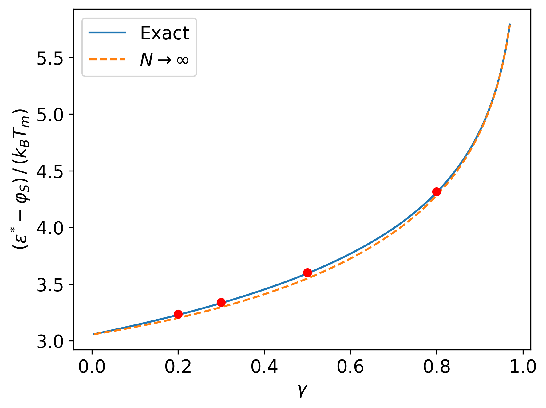
Figure 2: Ratio between the melting energy and temperature, according to (45) (solid blue line) and its approximation (47) (orange dashed line). Red circles indicate the values $\gamma$=0.2, 0.3, 0.5 and 0.8.

and also for $k_{B}T_{m}\ll\phi_{c}$. Fig. 2 shows the dimensionless intensive quantity

$$\zeta\mathrel{\mathop{:}}=\frac{\varepsilon^{*}-\varphi_{S}}{k_{B}T_{m}}$$

as a function of $\gamma$, using the approximation in (47) and the exact value in (45).

5 The caloric curve in the microcanonical ensemble

Just as we used the configurational partition function in Section  4 to compute the canonical caloric curve, we can use the full density of states $\Omega(E)$ to obtain the microcanonical caloric curve, being given in terms of the CDOS as

$$\begin{split}\eta(E)&=\int_{0}^{E}d\phi\mathcal{D}(\phi)\big{(}E-\phi\big{)}^{\frac{3N}{2}-1}=E^{\frac{3N}{2}-1}\int_{0}^{E}d\phi\mathcal{D}(\phi)\Big{(}1-\frac{\phi}{E}\Big{)}^{\frac{3N}{2}-1}\\ &=E^{\frac{3N}{2}-1}\left[\int_{0}^{\min(E,1)}d\phi\Big{(}1-\frac{\phi}{E}\Big{)}^{\frac{3N}{2}-1}\phi^{\alpha_{S}}+\frac{\Theta(E-1)}{(1-\gamma)^{\alpha_{L}}}\int_{1}^{E}d\phi\Big{(}1-\frac{\phi}{E}\Big{)}^{\frac{3N}{2}-1}(\phi-\gamma)^{\alpha_{L}}\right]\\ &=E^{C_{S}}B_{S}\Big{(}\textstyle 0\rightarrow\min(1,\frac{1}{E})\Big{)}+\displaystyle\frac{\Theta(E-1)}{(1-\gamma)^{\alpha_{L}}}(E-\gamma)^{C_{L}}B_{L}\Big{(}\lambda(E)\rightarrow 1\Big{)}\end{split}$$ (49)

where we have defined the auxiliary functions

$$\lambda(E)\mathrel{\mathop{:}}=\frac{1-\gamma}{E-\gamma}$$ (50)

and

$$B_{\nu}(a\rightarrow b)\mathrel{\mathop{:}}=\int_{a}^{b}dt\;t^{\alpha_{\nu}+1}(1-t)^{\frac{3N}{2}-1}$$ (51)

for convenience of notation, where $\nu=S,L$ and $a,b\in[0,1]$. Replacing in (49) we obtain $\eta(E)$ as a piecewise function,

$$\eta(E)=\begin{cases}E^{C_{S}}B(\alpha_{S}+1,\textstyle\frac{3N}{2})\;\text{for}\;E\leq 1\\[15.0pt] \displaystyle E^{C_{S}}B_{S}(0\rightarrow\textstyle\frac{1}{E})\displaystyle+\frac{(E-\gamma)^{C_{L}}}{(1-\gamma)^{\alpha_{L}}}B_{L}(\lambda(E)\rightarrow 1)\;\text{for}\;E>1.\end{cases}$$ (52)

We can see that the microcanonical inverse temperature for the branch with $E\leq 1$ is simply given by

$$\beta_{\text{low}}(E)=\frac{\partial}{\partial E}\ln(E^{C_{S}})=\frac{C_{S}}{E},$$ (53)

that is $E$ as a function of $T(E)$ is a straight line with slope $C_{S}$, in agreement with the low temperature approximation $E_{S}(T)$ of the canonical caloric curve in (29). This means the non-monotonic behavior, i.e. the van der Waals loop and the microcanonical melting energy $E_{m}$ must ocurr above $E=1$. Just as we did for the canonical ensemble, we will define the probabilities of solid and liquid, $P(S|E)$ and $P(L|E)$ respectively, at an energy $E\geq 1$, according to

$$P(S|E) \mathrel{\mathop{:}}=\frac{1}{\eta(E)}\int_{0}^{1}d\phi\mathcal{D}(\phi)(E-\phi)^{\frac{3N}{2}-1}=\frac{E^{C_{S}}B_{S}(0\rightarrow 1/E)}{\eta(E)},$$ (54)

$$P(L|E) \mathrel{\mathop{:}}=\frac{1}{\eta(E)}\int_{1}^{E}d\phi\mathcal{D}(\phi)(E-\phi)^{\frac{3N}{2}-1}=\frac{(E-\gamma)^{C_{L}}}{(1-\gamma)^{\alpha_{L}}}\frac{B_{L}(\lambda(E)\rightarrow 1)}{\eta(E)}.$$ (55)

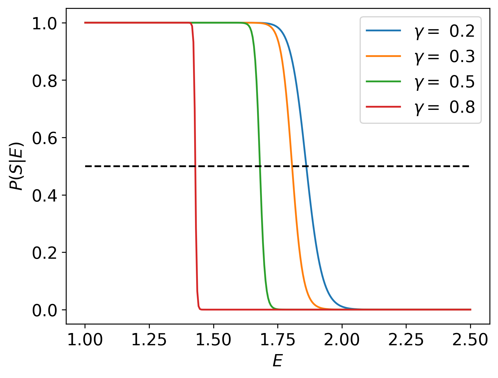
Figure 3: Microcanonical probability of solid phase $P(S|E)$ as a function of energy, for different values of $\gamma$.

The probability of solid is shown, as a function of energy, in Fig.  3. We will define the microcanonical melting energy $E_{m}$ as the value of $E$ such that $P(S|E_{m})=P(L|E_{m})$, being then the solution of the transcendental equation

$$(E_{m})^{C_{S}}(1-\gamma)^{\alpha_{L}}B_{S}(0\rightarrow 1/E_{m})=(E_{m}-\gamma)^{C_{L}}B_{L}(\lambda(E_{m})\rightarrow 1).$$ (56)

Using the derivatives

$$\frac{\partial}{\partial E}B_{S}(0\rightarrow 1/E) =\frac{\partial}{\partial E}\int_{0}^{1}dt\>t^{\alpha_{S}+1}(1-t)^{\frac{3N}{2}-1}\Theta(1/E-t)=-E^{-(C_{S}+2)}(E-1)^{\frac{3N}{2}-1}$$ (57)

$$\frac{\partial}{\partial E}B_{L}(\lambda(E)\rightarrow 1) =\frac{\partial}{\partial E}\int_{0}^{1}dt\>t^{\alpha_{L}+1}(1-t)^{\frac{3N}{2}-1}\Theta(t-\lambda(E))=\frac{1}{1-\gamma}\left[\lambda(E)^{\alpha_{L}+3}-\lambda(E)^{C_{L}+2}\right],$$ (58)

we can write

$$\eta^{\prime}(E)=\eta(E)\left(\frac{C_{S}}{E}P(S|E)+\frac{C_{L}}{E-\gamma}P(L|E)\right)+\lambda(E)^{2}\left[(E-\gamma)^{\frac{3N}{2}}-(1-\gamma)^{\frac{3N}{2}}\right]-E^{-2}(E-1)^{\frac{3N}{2}-1}$$ (59)

and then

$$\beta_{\text{high}}(E)=\left(\frac{C_{S}}{E}\right)P(S|E)+\left(\frac{C_{L}}{E-\gamma}\right)\big{(}1-P(S|E)\big{)}+\beta_{\text{res}}(E)$$ (60)

where

$$\beta_{\text{res}}(E)\mathrel{\mathop{:}}=\frac{1}{\eta(E)}\left(\lambda(E)^{2}\left[(E-\gamma)^{\frac{3N}{2}}-(1-\gamma)^{\frac{3N}{2}}\right]-\frac{1}{E^{2}}(E-1)^{\frac{3N}{2}-1}\right)$$ (61)

from which we see that the (inverse) temperature is also continuous at $E=1$. Similarly to $E_{\text{res}}(\beta)$ in the canonical ensemble, we can also see that $\beta_{\text{res}}(E)$ vanishes for both $E\rightarrow 1$ and $E\rightarrow\infty$. By using the Stirling approximation on the representation of the Beta function written in terms of $\Gamma$-functions,

$$B(x,y)=\frac{\Gamma(x)\Gamma(y)}{\Gamma(x+y)}\approx\sqrt{2\pi}\>\left[\frac{x^{x-1/2}y^{y-1/2}}{(x+y)^{x+y-1/2}}\right]$$ (62)

for large $x$ and $y$ we have

$$B_{\nu}(a\rightarrow b)\approx\begin{cases}K_{\nu}\;\text{if}\;\alpha_{\nu}/C_{\nu}\in[a,b]\\[10.0pt] 0\;\text{otherwise},\end{cases}$$ (63)

where

$$K_{\nu}\mathrel{\mathop{:}}=\sqrt{2\pi}\>\left[\frac{(\alpha_{\nu}+2)^{\alpha_{\nu}+3/2}{\Big{(}\tfrac{3N}{2}\Big{)}}^{3N/2-1/2}}{(C_{\nu}+1)^{C_{\nu}-1/2}}\right].$$ (64)

The probability of solid phase $P(S|E)$ is then approximated by

$$P(S|E)\approx\frac{E^{C_{S}}(1-\gamma)^{\alpha_{L}}K_{S}\mathrm{Q}[E\leq c_{S}/a_{S}]}{E^{C_{S}}(1-\gamma)^{\alpha_{L}}K_{S}\mathrm{Q}[E\leq c_{S}/a_{S}]+(E-\gamma)^{C_{L}}K_{L}\mathrm{Q}[E\geq\gamma+(c_{L}/a_{L})(1-\gamma)]}$$ (65)

where $\mathrm{Q}(A)$ is the indicator function [22] of the proposition $A$, defined as

$$\mathrm{Q}(A)=\begin{cases}1\;\;\text{if}\;A\;\text{is true},\\ 0\;\;\text{otherwise}.\end{cases}$$ (66)

Therefore, in this approximation the transition energy $E_{m}$, such that $P(S|E_{m})=1/2$, must be the solution of

$$E_{m}^{C_{S}}(1-\gamma)^{\alpha_{L}}K_{S}=(E_{m}-\gamma)^{C_{L}}K_{L}$$ (67)

provided that no indicator function vanishes, that is, it must hold that

$$\gamma+\frac{c_{L}}{a_{L}}(1-\gamma)\leq E_{m}\leq\frac{c_{S}}{a_{S}}.$$ (68)

These inequalities impose a lower limit on $\gamma$, namely

$$\gamma\geq\frac{a_{L}}{a_{S}}-1,$$ (69)

which however is only relevant if $a_{L}>a_{S}$, as it prevents $\gamma$ for reaching zero. In order to determine the solutions $E^{*}$ corresponding to the maximum and minimum of microcanonical temperature, we impose

$$\frac{\partial}{\partial E}\beta(E)\Big{|}_{E=E^{*}}=\frac{\partial^{2}}{\partial E^{2}}\ln\eta(E)\Big{|}_{E=E^{*}}=\frac{\eta^{\prime\prime}(E^{*})}{\eta(E^{*})}-\left(\frac{\eta^{\prime}(E^{*})}{\eta(E^{*})}\right)^{2}=0,$$ (70)

therefore

$$\eta^{\prime\prime}(E^{*})\cdot\eta(E^{*})=\eta^{\prime}(E^{*})^{2}.$$ (71)

The exact conditions under which (71) has exactly two solutions remain to be explored. Nevertheless, we have verified this fact numerically, and in Fig. 4 the green diamonds show the numerical solutions of (71) using the expression (52) for $\eta(E)$ in the case $E>1$, together with the canonical and microcanonical caloric curves. The ensemble inequivalence expected in small systems [23] is clearly seen, and a rather remarkable agreement of the microcanonical curves with the usual shape of the Z curves in the literature is found. The degree of superheating increases with $\gamma$, and the van der Waals loop typically found in microcanonical curves of small systems [24, 25, 26, 27, 28, 29, 30] gradually becomes sharper. However, the lower inflection point in the microcanonical curve does not coincide with the value of $T_{m}$ obtained from the canonical curve, suggesting that the model for the CDOS could be improved by adding additional parameters.

6 Concluding remarks

We have presented a study of the microcanonical and canonical melting curves for a simple solid, based on the recently proposed model in Ref. [14]. Our results show that this model is sufficient to reproduce the existence of superheating and recover the so-called Z curves of microcanonical melting, in which the Z-method by Belonoshko et al [1] is based. This is a first step for an explanation of the foundations of the Z-method in terms of ensemble inequivalence for small systems.

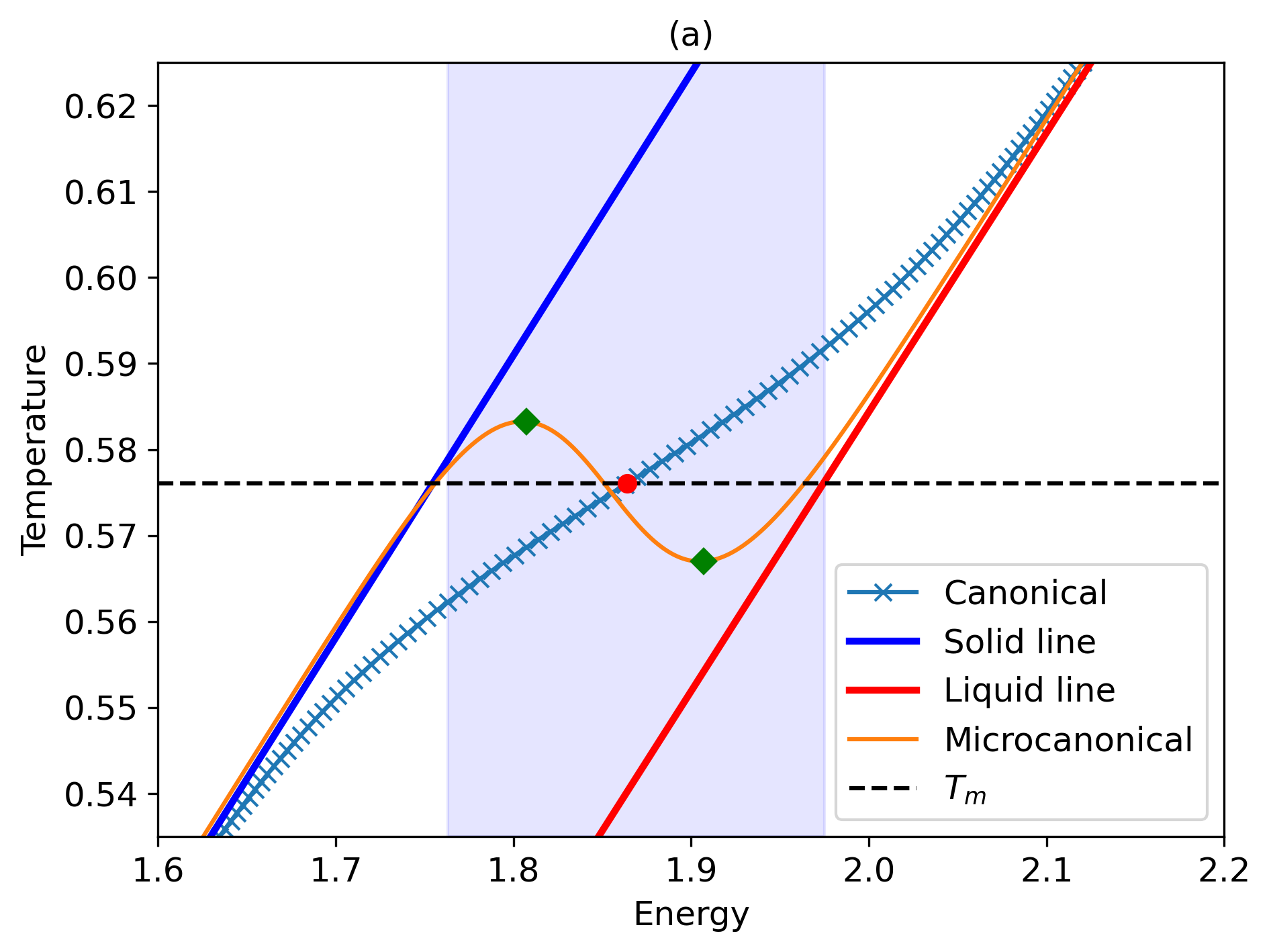
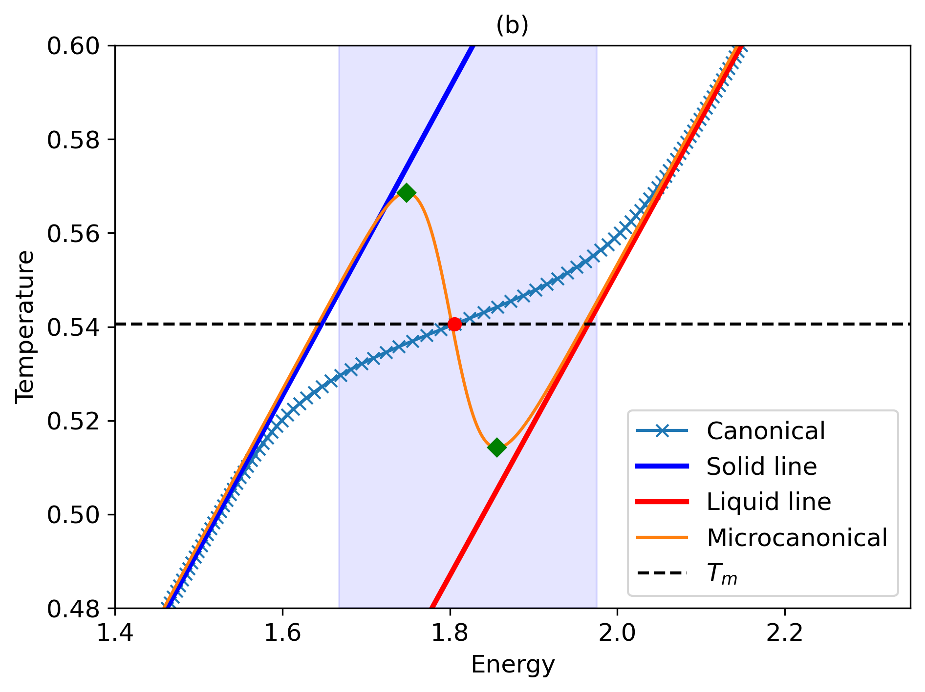
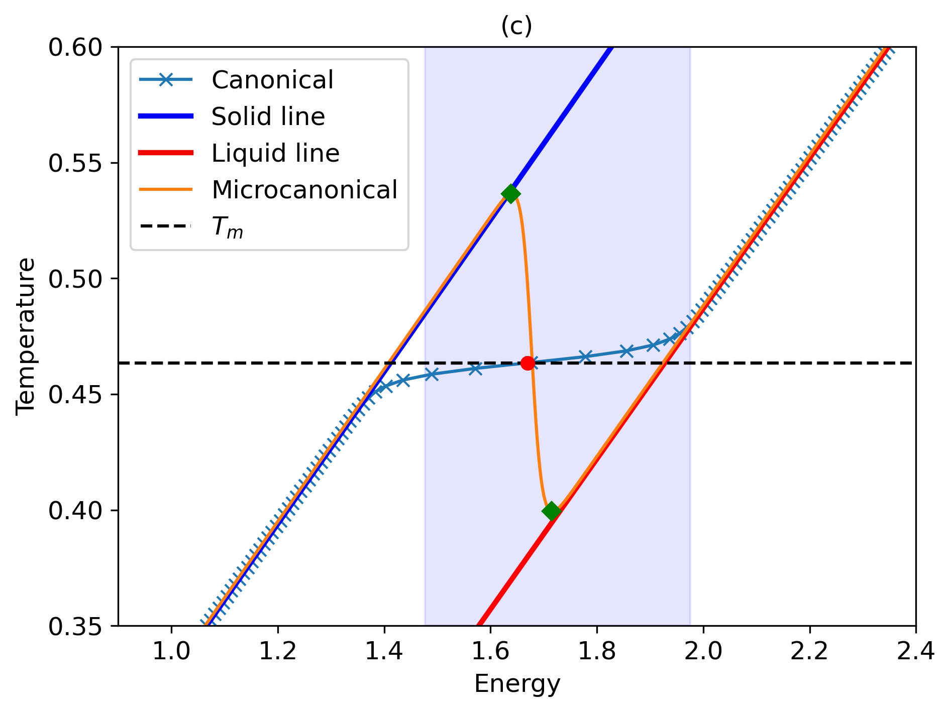
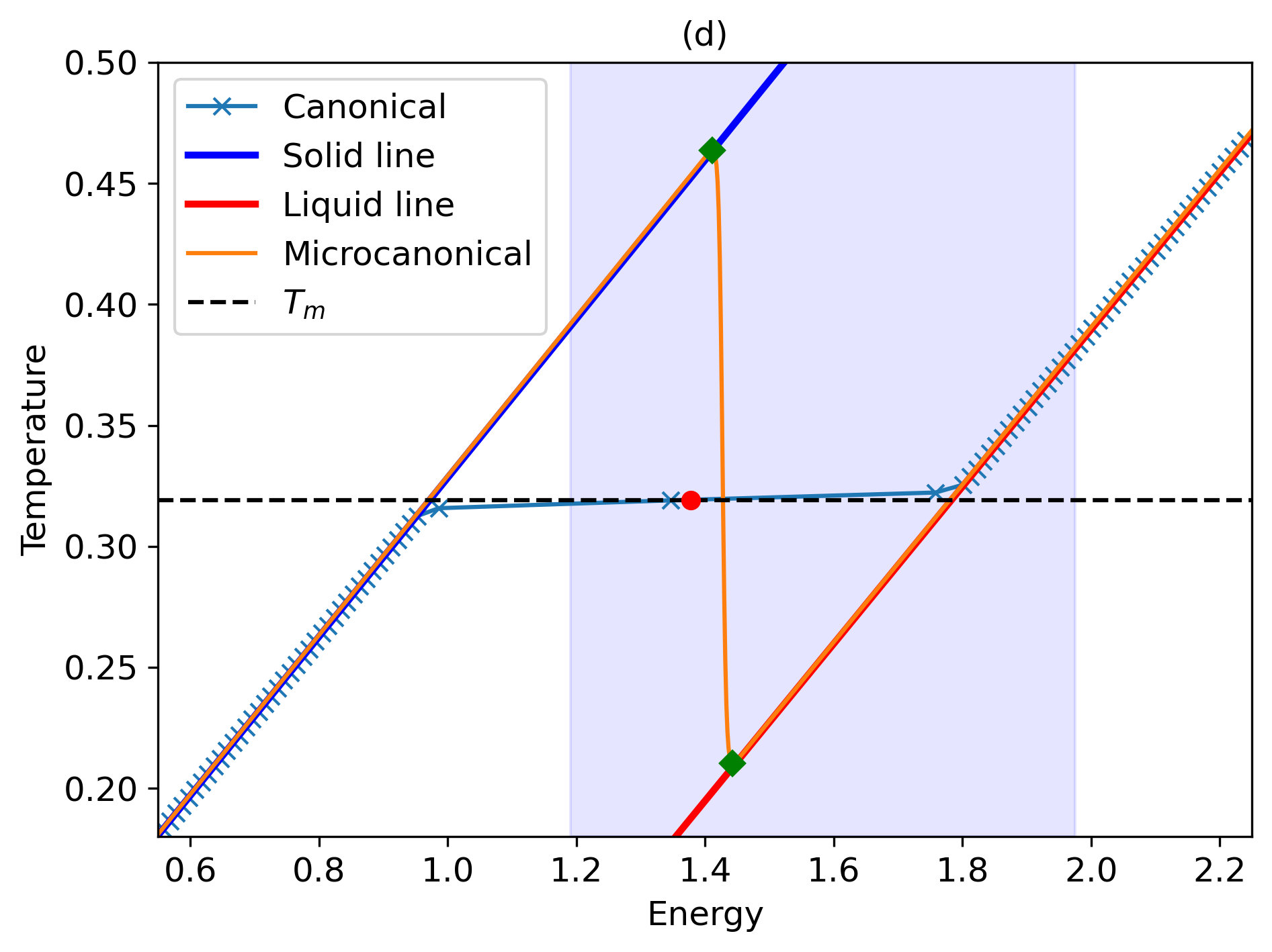
Figure 4: Canonical and microcanonical isochoric curves for $N$=128, $\alpha_{S}/N$ = 1.53812 and $\alpha_{L}/N$ = 1.57241, with (a) $\gamma$=0.2, (b) $\gamma$=0.3, (c) $\gamma$=0.5 and (d) $\gamma$ = 0.8.

References

- [1] A. B. Belonoshko, N. V. Skorodumova, A. Rosengren, and B. Johansson. Melting and critical superheating. Phys. Rev. B, 73:012201, 2006.
- [2] A. B. Belonoshko, S. Davis, N. V. Skorodumova, P. H. Lundow, A. Rosengren, and B. Johansson. Properties of the fcc Lennard–Jones crystal model at the limit of superheating. Phys. Rev. B, 76:064121, 2007.
- [3] J. Bouchet, F. Bottin, G. Jomard, and G. Zérah. Melting curve of aluminum up to 300 GPa obtained through ab initio molecular dynamics simulations. Phys. Rev. B, 80:94102, 2009.
- [4] D. F. Li, P. Zhang, J. Yan, and H. Y. Liu. Melting curve of lithium from quantum molecular-dynamics simulations. EPL, 95:56004, 2011.
- [5] A. B. Belonoshko and A. Rosengren. High-pressure melting curve of platinum from ab initio Z method. Physical Review B, 85:174104, 2012.
- [6] V. Stutzmann, A. Dewaele, J. Bouchet, F. Bottin, and M. Mezouar. High-pressure melting curve of titanium. Physical Review B, 92:224110, 2015.
- [7] F. González-Cataldo, S. Davis, and G. Gutiérrez. Melting curve of sio2 at multimegabar pressures: implications for gas giants and super-earths. Sci. Rep., 6:26537, 2016.
- [8] S. Anzellini, V. Monteseguro, E. Bandiello, A. Dewaele, L. Burakovsky, and D. Errandonea. In situ characterization of the high pressure–high temperature melting curve of platinum. Sci. Rep., 9:1–10, 2019.
- [9] D. Errandonea, L. Burakovsky, D. L. Preston, S. G. MacLeod, D. Santamaría-Perez, S. Chen, H. Cynn, S. I. Simak, M. I. McMahon, J. E. Proctor, et al. Experimental and theoretical confirmation of an orthorhombic phase transition in niobium at high pressure and temperature. Communications Materials, 1:1–11, 2020.
- [10] P. Mausbach, R. Fingerhut, and J. Vrabec. Structure and dynamics of the Lennard-Jones fcc-solid focusing on melting precursors. J. Chem. Phys., 153:104506, 2020.
- [11] S. R. Baty, L. Burakovsky, and D. Errandonea. Ab initio phase diagram of copper. Crystals, 11:537, 2021.
- [12] S. Davis, A. B. Belonoshko, B. Johansson, and A. Rosengren. Model for diffusion at the microcanonical superheating limit from atomistic computer simulations. Phys. Rev. B, 84:064102, 2011.
- [13] V. Olguín-Arias, S. Davis, and G. Gutiérrez. Extended correlations in the critical superheated solid. J. Chem. Phys., 151:064507, 2019.
- [14] A. Montecinos, C. Loyola, J. Peralta, and S. Davis. Microcanonical potential energy fluctuations and configurational density of states for nanoscale systems. Phys. A, 562:125279, 2021.
- [15] I. H. Umirzakov. van der Waals type loop in microcanonical caloric curves of finite systems. Phys. Rev. E, 60:7550–7553, 1999.
- [16] M. Kardar. Statistical Physics of Particles. Cambridge University Press, 2007.
- [17] E. M. Pearson, T. Halicioglu, and W. A. Tiller. Laplace-transform technique for deriving thermodynamic equations from the classical microcanonical ensemble. Phys. Rev. A, 32:3030–3039, 1985.
- [18] J. R. Ray. Microcanonical ensemble Monte Carlo method. Phys. Rev. A, 44:4061–4064, 1991.
- [19] M. A. Carignano. Monte Carlo simulations of small water clusters: microcanonical vs canonical ensemble. Chem. Phys. Lett., 361:291–297, 2002.
- [20] S. Davis. Calculation of microcanonical entropy differences from configurational averages. Phys. Rev. E, 84:50101, 2011.
- [21] S. Davis, J. Peralta, Y. Navarrete, D. González, and G. Gutiérrez. A Bayesian interpretation of first-order phase transitions. Found. Phys., 46:350–359, 2016.
- [22] G. Grimmett and D. Welsh. Probability: An Introduction. Oxford University Press, 2014.
- [23] J. Dunkel and S. Hilbert. Phase transitions in small systems: Microcanonical vs. canonical ensembles. Phys. A, 370:390–406, 2006.
- [24] J. P. K. Doye and D. J. Wales. Calculation of thermodynamic properties of small Lennard-Jones clusters incorporating anharmonicity. J. Chem. Phys., 102:9659–9672, 1995.
- [25] M. Schmidt, R. Kusche, T. Hippler, W. Kronmüller, B. von Issendorff, and H. Haberland. Negative heat capacity for a cluster of 147 sodium atoms. Physical Review Letters, 86:1191, 2001.
- [26] H. Behringer, M. Pleimling, and A. Huller. Finite-size behaviour of the microcanonical specific heat. J. Phys. A: Math. Theor., 38:973–985, 2005.
- [27] H. Behringer and M. Pleimling. Continuous phase transitions with a complex dip in the microcanonical entropy. Phys. Rev. E, 74:011108, 2006.
- [28] M. Eryürek and M. H. Güven. Negative heat capacity of Ar55 cluster. Physica A, 377:514–522, 2007.
- [29] M. Eryürek and M. H. Güven. Peculiar thermodynamic properties of LJN (=39-55) clusters. European Physical Journal D, 48:221–228, 2008.
- [30] M. A. Carignano and I. Gladich. Negative heat capacity of small systems in the microcanonical ensemble. EPL, 90:63001, 2010.