Equilibrium points and their linear stability in the planar equilateral restricted four-body problem: A review and new results

Abstract.

In this work, we revisit the planar restricted four-body problem to study the dynamics of an infinitesimal mass under the gravitational force produced by three heavy bodies with unequal masses, forming an equilateral triangle configuration. We unify known results about the existence and linear stability of the equilibrium points of this problem which have been obtained earlier, either as relative equilibria or a central configuration of the planar restricted $(3+1)$-body problem. It is the first attempt in this direction. A systematic numerical investigation is performed to obtain the resonance curves in the mass space. We use these curves to answer the question about the existing boundary between the domains of linear stability and instability. The characterization of the total number of stable points found inside the stability domain is discussed.

1. Introduction

The Newtonian planar $n$-body problem reads as the study of the dynamics of $n$ point particles with masses $m_{i}$ and positions$q_{i}$, $i=1,\dots,n$, moving according to Newton’s law of motion.

The equations of motion of the $n$-body problem are

(1) $$m_{j}\ddot{q}_{j}=\sum_{i\neq j}\frac{m_{i}m_{j}(q_{i}-q_{j})}{r_{ij}^{3}},\qquad 1\leq j\leq n.$$

where $r_{ij}=|q_{i}-q_{j}|$ is the Euclidean distance between $q_{i}$ and $q_{j}$, and we have chosen the units of length in order that the gravitational constant be equal to one. Let $q=(q_{1},\dots,q_{n})$ be the $2n$-dimensional configuration vector of the primary bodies.

In the planar Newtonian $n$-body problem the simplest motions, called homographic solutions, are such that the configuration is constant up to rotation and scaling. Relative equilibria are homographic solutions with the property that the system rotates about its center of mass $c\in{\mathbb{R}}^{2}$ as a rigid body and its angular velocity $\omega\neq 0$ is constant. In a rotating coordinate system they become equilibrium solutions of the $n$-body problem, hence the name. Such a solution is possible if and only if the initial positions $q_{i}(0)$ satisfy the algebraic equations

(2) $$\lambda(q_{j}-c)=\sum_{i\neq j}\frac{m_{i}m_{j}(q_{i}-q_{j})}{r_{ij}^{3}},\qquad 1\leq j\leq n,$$

for some a positive constant $\lambda$.

A configuration $q=(q_{1},\dots,q_{n})\in{\mathbb{R}}^{2n}$ of the planar $n$-body problem, satisfying (2), is called a central configuration. As a consequence, a relative equilibrium is a central configuration that rigidly rotates about its center of mass. The reader is addressed to Chapter 2 of [18] for a thorough treatment of this topic.

The number of central configurations of the planar $n$-body problem for an arbitrary given set of positive masses have long been established only for $n=3$. Up to rotations and translations, there are always exactly five classes of central configurations for each choice of positive masses: Two of these are three bodies of arbitrary mass located at the vertices of an equilateral triangles (Lagrange’s solutions) and the remaining three are collinear central configurations (Euler’s solutions). However, a complete classification is not known for $n>3$. Even the finiteness of the central configurations is a very difficult question. For the general four-body problem, the finiteness of the relative equilibria was settled by Hampton and Moeckel [14]. They showed that there are at least 32 and at most 8472 such equivalence classes, including the 12 collinear ones.

A special case of the $n$-body problem is the limiting case in which one of the masses tends to zero. In the planar restricted ($N+1$)-body problem, one is asked to consider the motion of a particle of infinitesimal mass moving in the plane under the influence of the gravitational attraction of $N$ finite particles (called primaries) that move around their common center of mass by retaining an orbit solution of the $N$-body problem. The infinitesimal mass body is supposed to have no gravitational effect on the other $N$ bodies.

In what follows, we will focus on the planar, circular, restricted four-body problem, where the three bodies with positive mass are located at the vertices of an equilateral triangle (Lagrange’s central configuration) rotating on circular orbits about their common center of mass. We will refer to this problem as the planar, equilateral, restricted four-body problem, hereafter ERFBP. This problem originates from the work of Pedersen [19].

The contribution in this paper is twofold. First, we shall give a state-of-the-art review of count, location and linear stability of the equilibria in the ERFBP. We then provide new contributions found by us concerning to the boundary between the domains of linear stability and instability of the full set of equilibrium points of the ERFBP in the rotating frame.

Before going into this, it is worth noting that one difficulty in counting the exact number of equilibrium points (relative equilibrium or central configuration) is due to the bifurcations. Thus, some others interesting papers dealing with the equilibrium set and its bifurcations should be mentioned.

There has been a substantial amount of analytic and numerical work involving the number of equilibria of the ERFBP. In order to be self-contained and to make this paper easily understandable to the reader, we summarize briefly some known results about equilibrium points of the ERFBP.

We start with the work by Pedersen [19], who made a combination of numerical and analytical methods to compute the number and positions of equilibrium points for the infinitesimal mass of the ($1+3$)-body problem, when the three large masses form a Lagrangian equilateral triangle. He found that, there can be 8, 9, or 10 equilibrium positions, depending on the values of the primary masses. Moreover, Pedersen proved that the set of degenerate equilibrium points is a simple closed curve contained in the interior of the triangle of positive masses, namely in the simplex $\Sigma$ in the masas space (that will appear later in this work). Here, we will denote this curve by $\mathfrak{B}$. He proved that, on the bifurcation curve $\mathfrak{B}$, there are 9 equilibrium points. Pedersen’s numerical calculations were later confirmed in a paper due to Simó [22], where a numerical study was done for the number of relative equilibrium solutions in the four-body problem for arbitrary masses.

In [3], Arenstorf outlines some analytical proofs of the main results contained in [19]. In the last part of his paper, he emphasizes that a careful mathematical analysis and rigorous calculations required to prove these results are contained in the Ph.D. thesis of his student Gannaway [12]. As it turns out, in Gannaway’s dissertation, there are only a few analytical evidences for particular assertions. Nevertheless, most of Pedersen’s substantial affirmations about central degenerate configurations, bifurcations and counting are verified once again only by a thorough numerical analysis. These studies were eventually completed by Barros and Leandro [6, 7]. They were able to give a mathematically rigorous computer-assisted proof proving that, $\mathfrak{B}$ is a simple, closed, continuous curve, which lies inside the triangle $\Sigma$ formed by the positive masses. Besides, Leandro and Barros also confirmed that there are either 8, 9, or 10 equilibrium solutions (depending on the primary masses), and proved that 6 of them are outside of the Lagrange equilateral triangle formed by the primary bodies. Recently, Figueras et al. [11] gave a new proof to the one performed by Barros and Leandro [6, 7], which is also based on computer-assisted methods, but they applied real analysis techniques instead of (complex) algebraic geometry to counting relative equilibria in the ERFBP. In contrast to the original proof by Leandro and Barros, their proof does not require any difficult computation.

The finiteness of the number of equilibria (central configurations) in the ERFBP is demonstrated by Kulevic et al. [15]. They used tools from algebraic geometry to state that the number of equilibria in the ERFBP is finite for any choice of masses, and is bounded above by 196. However, they claim that most of these solutions of the equilibrium equations found by them, are physically meaningless. The numerical simulations suggest that the true number varies from 8 and 10, depending on the masses. These lower estimates are just as described on [19], [3], [12], [22], [4], [16], [6], [7], [24], [11].

On the other side, the paper by Baltagiannis and Papadakis [4], one of the recent works we consider in this article, the authors provided an extended list of possible combinations of primary bodies masses and their respective number of points of equilibrium. Other works related to ours are Budzco and Prokopeny [9] and Zepeda Ramírez et al. [23], where the authors study the non-linear stability in the case when the mass parameters of the system lie inside the domain of linear stability points. In the same vein, we will review a recent work by Zotos [24] where previously known results are retrieved.

It should be noted that, in contrast to the restricted three-body problem, the ERFBP with total mass normalized to one, has two parameters masses, and due to this reason the calculations are much larger and difficult to carry out. With the approach followed in the present paper, we are able to verify that the number and stability of the equilibria depend on mass parameters of the primary bodies in a continuous way, as seen in previous papers.

This paper is organized as follows. In Section 2, the problem and equations of motion are presented. In Section 3 the existence and position of the equilibrium points are investigated, while Section 4 is devoted to analyze their linear stability. We quote some of the classic results and some recent. The list does not include all the issues but they are rather significant. A careful numerical analysis allow us to conclude that resonance curves play a key role in determining the stability domain, whose border is given by the $1$:$1$ resonance curve. Actually, this occurs within and near the three triangular regions in the mass space where the Lagrangian relative equilibria are stable. The knowledge of resonance curves leads us to clarify some points that are a little bit obscure in [24]. In Section 5 we outline some conclusions.

Finally, we stress that all our numerical calculations and graphs of the obtained results have been performed with the Mathematica software.

2. Description of the problem

The Newtonian planar equilateral restricted four-body problem describes the motion of an infinitesimal particle under the gravitational attraction of three primaries $m_{1}$, $m_{2}$ and $m_{3}$ arranged in a central configuration of Lagrange, so that the masses are at the vertices of a rotating equilateral triangle, where the rotation has constant angular velocity $\omega$.

Since the equilateral central configuration is possible for all distributions of masses, this paper considers the ERFBP where the primaries are assumed to have arbitrary masses which are normalized so that the total mass of the primaries is taken as the unit of mass, that is, $m_{1}+m_{2}+m_{3}=1$. Hence, the number of mass parameters is reduced from three to two.

Under the assumption that the center of mass is at the origin of the coordinate system, the dynamics of the infinitesimal particle $m$, the system is referred to a rotating (also called synodical) coordinate frame $(x,y)$, with uniform angular velocity. We orient the triangular configuration so that $m_{1}$ lies on the positive $x$-axis, whose geometry is illustrated in Figure 1.

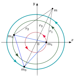
Figure 1. The equilateral restricted four-body problem in a sidereal frame of reference.

Define $K=m_{2}(m_{3}-m_{2})+m_{1}(m_{2}+2m_{3})$. In the synodic reference frame, the coordinates $(x_{1},y_{1})$, $(x_{2},y_{2})$ and $(x_{3},y_{3})$ of the primaries are given by

$$x_{1}=\frac{|K|\sqrt{m^{2}_{2}+m_{2}m_{3}+m^{2}_{3}}}{K}, y_{1}=0,$$

$$x_{2}=-\frac{|K|\left[(m_{2}-m_{3})m_{3}+m_{1}(2m_{2}+m_{3})\right]}{2K\sqrt{m^{2}_{2}+m_{2}m_{3}+m^{2}_{3}}}, y_{2}=\frac{\sqrt{3}}{2}\frac{m_{3}}{m^{3/2}_{2}}\sqrt{\frac{m^{2}_{2}}{m^{2}_{2}+m_{2}m_{3}+m^{2}_{3}}},$$

$$x_{3}=-\frac{|K|}{2\sqrt{m^{2}_{2}+m_{2}m_{3}+m^{2}_{3}}}, y_{3}=-\frac{\sqrt{3}}{2}\frac{1}{m^{1/2}_{2}}\sqrt{\frac{m^{2}_{2}}{m^{2}_{2}+m_{2}m_{3}+m^{2}_{3}}}.$$

The equations of motion of the infinitesimal mass $m$ are written as

(3) $$\begin{array}[]{l}\ddot{x}-2\dot{y}=\Omega_{x},\vspace{0.3cm}\\ \ddot{y}+2\dot{x}=\Omega_{y},\end{array}$$

where dots denote derivatives with respect to time $t$, and

(4) $$\Omega=\Omega(x,y)=\frac{1}{2}(x^{2}+y^{2})+\frac{m_{1}}{r_{1}}+\frac{m_{2}}{r_{3}}+\frac{m_{3}}{r_{2}}$$

is the potencial function with $r_{1}=\sqrt{(x-x_{1})^{2}+y^{2}}$, $r_{2}=\sqrt{(x-x_{2})^{2}+(y-y_{2})^{2}}$ and $r_{3}=\sqrt{(x-x_{3})^{2}+(y-y_{3})^{2}}$.

The Hamiltonian governing the motion of the infinitesimal particle in these coordinates is

(5) $$H=\frac{1}{2}(p^{2}_{x}+p^{2}_{y})+yp_{x}-xp_{y}-U(x,y),$$

where $p_{x}=\dot{x}-y$ and $p_{y}=\dot{y}+x$ are the conjugate momenta, and

$$U(x,y)=\frac{m_{1}}{r_{1}}+\frac{m_{2}}{r_{2}}+\frac{m_{3}}{r_{2}}$$

is the self-potential.

At this time the reader should be warned that the condition $m_{1}+m_{2}+m_{3}=1$ implies that ERFBP depends only on two mass parameters. In particular, we take $m_{3}=1-m_{1}-m_{2}$ with $m_{1}\neq m_{2}\neq m_{3}$, so the two free parameters will be $m_{1}$ and $m_{2}$. According to Gaschea [13] and Routh [21], the triangle configuration of the primaries is stable only when the Routh’s stability condition given by inequality

(6) $$\frac{m_{1}m_{2}+m_{1}m_{3}+m_{2}m_{3}}{(m_{1}+m_{2}+m_{3})^{2}}<\frac{1}{27}$$

is fulfilled. Indeed, this inequality is satisfied only if one mass of the primaries dominates over the other masses. Figure 2 depicts the stability regions on the $(m_{1},m_{2})$ plane, when both inequalities $m_{1}m_{2}+m_{2}m_{3}+m_{3}m_{1}<1/27$ (with $m_{3}=1-m_{1}-m_{2}$) and $m_{1}+m_{2}<1$ are true at the same time; the regions of stability are shown in the three gray-shaded areas and instability regions are shown in white, the red curves represent solutions to $m_{1}m_{2}+m_{2}m_{3}+m_{3}m_{1}=1/27$ and the dashed line represents the condition $m_{1}+m_{2}=1$. For convenience we label the gray-shaded areas of stability as follow: I for the lower left corner, II for the lower right corner and III for the upper left corner.

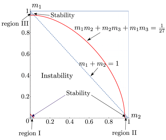
Figure 2. The three small “triangular" shaded regions I, II and III are stability domains of the Lagrange triangle configuration, and white region below the line $m_{1}+m_{2}=1$ is instability domain. The mass parameter of the third primary is $m_{3}=1-m_{1}-m_{2}$. The red lines correspond to the Routh’s critical curve.

We remark that, a simple calculation shows that region II can be obtained from III by means of reflection with respect to the line $m_{1}=m_{2}$. It follows that the set of masses on region II satisfy that $m_{1}$ and $m_{3}$ are very small with $m_{2}$ very large, while on region III $m_{2}$ and $m_{3}$ are very small and $m_{1}$ is very large.

At this stage we need to remind that the normalized mass space can be represented as the 2-simplex

$$\Sigma=\{(m_{1},m_{2},m_{3})\in\mathbb{R}^{3}_{+}\>\mid m_{1}+m_{2}+m_{3}=1,\;0\leq m_{k}\leq 1,\;k=1,2,3\},$$

see Figure 3. This is an equilateral triangle, whose edges have length $\sqrt{2}$ and it is called the triangle of masses. It can be seen as the barycentric coordinates of a point within $\Sigma$ are the masses $m_{1}$, $m_{2}$, $m_{3}$. The sides correspond to mass values of the (2 + 2)-body problem (two large and two massless), while the vertices are the masses of the (1 + 3)-body problem.

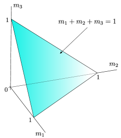
Figure 3. Parameter simplex $\Sigma$ in the mass space $(m_{1},m_{2},m_{3})$ normalized so that $m_{1}+m_{2}+m_{3}=1$. The simplex is formed by the vertices $(1,0,0)$, $(0,1,0)$ and $(0,0,1)$.

3. Equilibrium points

We now compute the equilibrium points of equations (3). By calculating the derivatives of (4) and equaling them to zero the equilibrium points coordinates $(x,y)$ are determined by

(7) $$\begin{array}[]{l}\displaystyle{\frac{\partial\Omega}{\partial x}=x-\frac{m_{1}(x-x_{1})}{[(x-x_{1})^{2}+y^{2}]^{3/2}}-\frac{m_{2}(x-x_{2})}{[(x-x_{2})^{2}+(y-y_{2})^{2}]^{3/2}}-\frac{m_{3}(x-x_{3})}{[(x-x_{3})^{2}+(y-y_{3})^{2}]^{3/2}}=0},\vspace{0.3cm}\\ \displaystyle{\frac{\partial\Omega}{\partial y}=y-\frac{m_{1}y}{[(x-x_{1})^{2}+y^{2}]^{3/2}}-\frac{m_{2}(y-y_{2})}{[(x-x_{2})^{2}+(y-y_{2})^{2}]^{3/2}}-\frac{m_{3}(y-y_{3})}{[(x-x_{3})^{2}+(y-y_{3})^{2}]^{3/2}}=0.}\end{array}$$

Since the system (7) is intractable analytically, the search of equilibrium solutions is achieved by means of numerical methods. An intuitive method to locate them relies on finding intersections of these zero velocity curves. We select two sets of mass parameters to plot the positions of the equilibrium points, through the mutual intersections of the zero velocity curves shown in Figure 4. The labeling for the equilibrium points as $L_{i}$, $i=1,2,\dots,10$ follows the notation stated in [4].

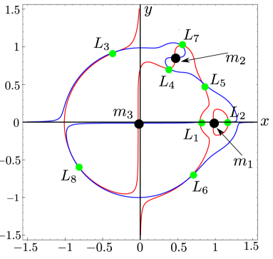
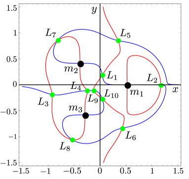
Figure 4. Equilibrium points in the $x$-$y$ plane located at the intersection of the curves $\Omega_{x}=0$ (red) and $\Omega_{y}=0$ (blue) for: (a) $m_{1}=0.02$ and $m_{2}=0.015$ with eight equilibria and (b) $m_{1}=0.4$ and $m_{2}=0.35$ with ten equilibria. The green dots denote the position of the equilibrium points and the positions of the primaries are marked by black dots.

In a recent paper by Zotos [24], a detailed numerical study was carried out to show the number and location of equilibrium points of the ERFBP, for all possible values of the masses of the primaries, as well as its bifurcation set. Since $m_{3}=1-m_{1}-m_{2}$, the results are presented in the simplex defined by $m_{1}+m_{2}<1$ with $0<m_{1},m_{2}<1$ on the $(m_{1},m_{2})$ plane, as in Figure 5. In fact, Zotos claims that in the red region there are 10 equilibrium points and in the green region there are only 8. Also, the bifurcation curve $\mathfrak{B}$ is depicted as the border of the central region colored as red, which is almost triangular shaped and cutting the simplex in two components. Unfortunately, it seems that Zotos was unaware that the coordinates, number and bifurcation curve $\mathfrak{B}$ of equilibrium points have been known from earlier works by, among others, [19], [22], [3], [12], [6] and [7].

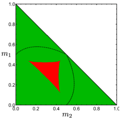
Figure 5. Regions on the $(m_{1},m_{2})$ plane, corresponding to eight (green) and ten (red) points of equilibrium. The black dashed lines are indicating the set of mass values on which the sign of the relative positions coordinates of the primaries $m_{1}$ and $m_{2}$ is changing. The border of the red region corresponds to the bifurcation curve $\mathfrak{B}$. This figure is taken from [24].

4. Linear stability of the equilibrium points

Once the coordinates of the equilibrium conditions $(x_{0},y_{0})$ have been determined, its linear stability can also be studied. We start by moving the equilibria to the origin of a coordinate system. Therefore, one sees that the characteristic equation can be written as:

(8) $$\lambda^{4}+(4-A_{11}-A_{22})\lambda^{2}+A_{11}A_{22}-A^{2}_{12}=0,$$

where

(9) $$\begin{array}[]{l}A_{11}=1+\displaystyle{\sum_{i=1}^{3}}\frac{m_{i}[2(x_{0}-x_{i})^{2}-(y_{0}-y_{i})^{2}]}{[(x_{0}-x_{i})^{2}-(y_{0}-y_{i})^{2}]^{5/2}},\vspace{0.3cm}\\ A_{12}=3\displaystyle{\sum_{i=1}^{3}}\frac{m_{i}[(x_{0}-x_{i})(y_{0}-y_{i})]}{[(x_{0}-x_{i})^{2}-(y_{0}-y_{i})^{2}]^{5/2}},\vspace{0.3cm}\\ A_{22}=1-\displaystyle{\sum_{i=1}^{3}}\frac{m_{i}[(x_{0}-x_{i})^{2}-2(y_{0}-y_{i})^{2}]}{[(x_{0}-x_{i})^{2}-(y_{0}-y_{i})^{2}]^{5/2}},\end{array}$$

with $m_{1}\neq m_{2}\neq m_{3}\neq 0$.

By virtue of Lyapunov’s theorem on stability of equilibria for autonomous Hamiltonian systems with two degrees of freedom (see [17]), we have that the equilibria are linearly stable if (8) has four pure imaginary roots. Indeed, this is secured by the three following conditions:

(10) $$\begin{array}[]{l}(4-A_{11}-A_{22})^{2}-4(A_{11}A_{22}-A_{12}^{2})\geq 0,\\ 4-A_{11}-A_{22}>0,\\ A_{11}A_{22}-A_{12}^{2}>0\end{array}$$

which must be fulfilled simultaneously, whose frequencies $\omega_{1}$ and $\omega_{2}$ are given by

$$\omega_{1,2}=\frac{1}{\sqrt{2}}\sqrt{-4+A_{11}+A_{22}\pm\sqrt{(4-A_{11}-A_{22})^{2}-4(A_{11}A_{22}-A_{12}^{2})}}.$$

It is known from numerical studies by, among others, Pedersen [19], Arenstorf [3], Simó [22] and Baltagiannis and Papadakis [4], that the region on the plane $(m_{1},m_{2})$ where the triangular configuration of the three primaries is stable, there exist eight equilibrium points. It is noteworthy that Barros and Leandro [7] used analytical and computational techniques to prove that, for all triples $(m_{1},m_{2},m_{3})\in\Sigma$ which are close enough to $\partial\Sigma$, the number of central configurations is eight. This means we will have eight equilibrium points on regions I, II and III.

We note the system of equations (7) is nonlinear, and we do not know, in advance, where the equilibrium points are located for different values of $m_{1}$ and $m_{2}$ with $m_{3}=1-m_{1}-m_{2}$. For this reason, in order to find the solutions of (7) as a function of the masses, we proceed to solve them numerically in the already mentioned region contained in the plane $m_{1}m_{2}$. To do so, we define a dense uniform grid with a small step, which correspond to the initial approximations in order to apply the command FindRoot built within the Mathematica software. Then, these solutions, and also the respective values of the masses, are inserted into the characteristic equation (8) and thus we derive its linear stability.

Numerical analysis of conditions (10) at each equilibrium point shows that $L_{1}$, $L_{2}$, $L_{4}$, $L_{7}$ and $L_{8}$ are unstable, while $L_{3}$, $L_{5}$ and $L_{6}$ are the only stable equilibria for any values of the masses from the regions where the Lagrange’s configuration is stable. This is in agreement with the results obtained by Simó [22], Budzko and Prokopenya [9], Baltagiannis and Papadakis [4] and Zotos [24], but some of them used different labels for the points, see Table 1.

Baltagiannis & Papadakis	Simó	Budzko & Prokopenya	Zotos
$L_{3}$	$L_{4}$	$S_{1}$	$L_{2}$
$L_{5}$	$L_{5}$	$S_{4}$	$L_{3}$
$L_{6}$	$L_{6}$	$S_{7}$	$L_{4}$

Table 1. Labels used to name the linear stable equilibrium points for several authors. We have opted the notation in the same way as Baltagiannis and Papadakis [4].

We stress that numerical evidence shows that, for arbitrary masses, the equilibrium points $L_{3}$ and $L_{5}$ are located in the upper half plane ($y>0$), also note that the position of $L_{6}$ is in the lower half plane ($y<0$); see, for instance Figure 4.

Next step is to build numerically the resonances between frequencies associated to the eigenvalues of the stable equilibrium points. We state the type and order of resonance for each one of the stable equilibria without regard to the stability of the triangle formed by the primaries. The corresponding curves are depicted in Figures 6, 7 and 8, respectively.

At this stage, we remind that region II can be obtained from region III by means of reflection with respect to the line $m_{1}=m_{2}$. Our computations show that, the stable equilibrium points in both regions are $L_{3}$, $L_{5}$ and $L_{6}$. In addition, the respective stability domains are symmetric with respect to the line $m_{1}=m_{2}$, respectively. Indeed, this is in agreement with the numerical results obtained by Zotos, which can be checked in the Figures 10(b) and 10(c) in [24].

Now, we would like to remark that lines $m_{2}=0$ ($m_{3}$-axis), $m_{3}=0$ ($m_{2}$-axis) and the line $m_{1}+m_{2}=1$ on the $m_{2}m_{1}$ plane correspond to two copies of the circular restricted three-body problem, respectively. Then, there are points of intersection of the resonance curves $1$:$1$, the curve $m_{1}m_{2}+m_{1}m_{3}+m_{2}m_{3}=1$ and either the axes or the line $m_{1}+m_{2}=1$. Those points are $R_{L_{3}}=(\mu_{R},0)$ in Figure 6 (a), $R_{L_{5}}=(\mu_{R},1-\mu_{R})$ in Figure 7 (b), $R_{L_{6}}=(0,\mu_{R})$ in Figure 8 (a), ${\mathcal{R}}_{L_{6}}=(\mu_{R},0)$ in Figure 8 (b), where $\mu_{R}=\frac{1}{2}(1-\sqrt{69}/9)\approx 0.038520896504551$ is the Routh’s critical mass ratio.

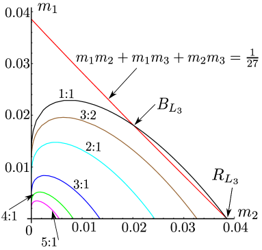
(a) Region I, $B_{L_{3}}=(0.02012014,0.018114)$.

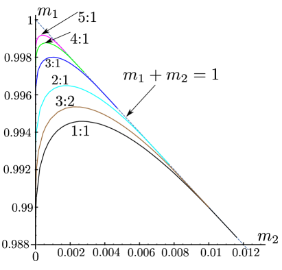
(b) Region III.

Figure 6. Resonance curves for the point $L_{3}$ in regions I and III.

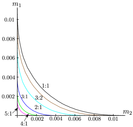
(a) Region I.

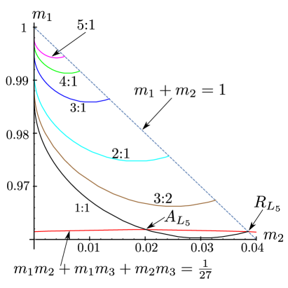
(b) Region III. $A_{L_{5}}=(0.02016,0.9619)$ and $R_{L_{5}}=(0.0385208,0.9614)=(\mu_{R},1-\mu_{R})$.

Figure 7. Resonance curves for equilibrium point $L_{5}$ in the regions I and III.

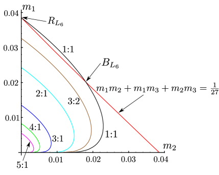
(a) Region I. $B_{L_{6}}=(0.018114,0.02012014)$ and $R_{L_{6}}=(0,0.0385208)=(0,\mu_{R})$.

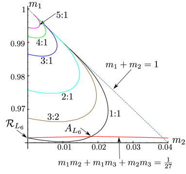
(b) Region III. $A_{L_{6}}=(0.01802,0.9619)$ and ${\mathcal{R}}_{L_{6}}=(0.9614,0.0385208)=(1-\mu_{R},\mu_{R})$.

Figure 8. Graphics of the resonance curves for equilibrium point $L_{6}$ on the regions I and III.

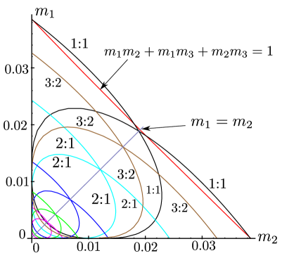
(a) Resonance curves in region I.

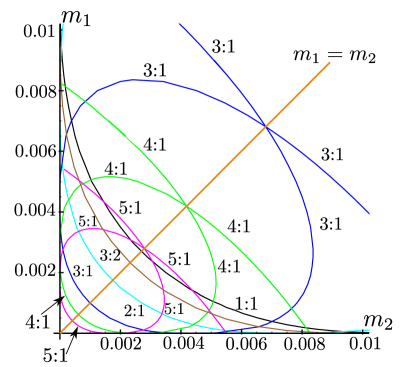
(b) The enlarged graph.

Figure 9. Plots of all resonance curves in region I for equilibrium points $L_{3}$, $L_{5}$ and $L_{6}$.

A striking observation is the fact that the regions where the points of equilibrium are linearly stable are bounded by the resonance curve $1$:$1$, that is, the stability domain is given by the values of $m_{1}$ and $m_{2}$ smaller than their values on the condition $\omega_{1}=\omega_{2}$. In a related approach to ours, Budzco [8] found equilibrium solutions and investigate their linear stability in the ERFBP and established that the stability boundaries are determined by the condition $\omega_{1}=\omega_{2}$, but he only considered the region I in his study. Later on, Budzco and Prokopenya [9] constructed curves on which the conditions of the third and fourth order resonances are fulfilled in the region I.

One must note that, equilibria $L_{3}$ and $L_{6}$ in region I, and also $L_{5}$ in regions II and III turn out to be linearly stable for some values of parameters $m_{1}$ and $m_{2}$ for which the Routh’s condition is not satisfied, then the Lagrange central configuration of the primaries is unstable. This fact was observed by Pedersen [20] who studies the stability of the $(3+1)$-body problem without regard to the stability of the primaries configuration. Also, this very same fact was obtained by Zotos [24]. The bifurcation values found by us are the following: for $L_{3}$ is $B_{L_{3}}=(0.02012014,0.018114)$, for $L_{5}$ is $A_{L_{5}}=(0.02016,0.9619)$, for $L_{6}$ are $B_{L_{6}}=(0.018114,0.02012014)$ and $A_{L_{6}}=(0.01802,0.9619)$. These are given in Figures 6(a), 7(b), 8(a) and 8(b), respectively.

To determine how many and which stable equilibrium points exist inside or outside regions I and III, we draw together the resonance curves of $L_{3}$, $L_{5}$ and $L_{6}$ in a single graph in Figures 9 and 10, respectively.

It is not a difficult task to establish a comparison between our numerical studies and those carried out by Zotos [24]. Figures 13(a) and 14(a) show the stability domains in regions I and III, respectively, their topology is exactly that one given by Zotos, but he did not identify the border of the domains, only stated the number of equilibrium points in each subregion and did not say to which point it corresponded. We go beyond this and are able to identify how many and what exactly are the respective stable points in the different subregions.

In Figure 11, we present all $1$:$1$ resonance curves in region I. On this basis, we note that there are two points of intersection of the resonance curve $1$:$1$ with the straight line $m_{1}=m_{2}$ (two primary bodies with equal masses). The first one is $A(0.002716,0.002716)$ that is precisely the point with resonance $1$:$1$ for $L_{5}$ where Burgos and Delgado [10] ($L_{2}$ in their notation) established the existence of a “blue sky catastrophe", and the other is $B(0.01883,0.01883)$ resonance values for $L_{3}$ and $L_{6}$, whose stability has not hitherto been studied. On the other side, the intersection point of the resonance curve $2$:$1$ with line $m_{1}=m_{2}$ in Figure 9 corresponds to the equilibrium where Alvarez-Ramírez et al. [2] studied the non-linear stability. Actually, similar points are found in region III. More precisely, we obtain the points by intersecting the resonance curves $1$:$1$ with the line $m_{1}=1-2m_{2}$, that means that $m_{2}=m_{3}$, namely $C(0.002736,0.994528)$ for $L_{3}$ and $D(0.01883,0.96234)$ for $L_{5}$ and $L_{6}$, see Figure 12. A novelty of this article lies in the fact that this is the first time that these points are obtained. It is interesting to note that in the region II are located the points with $m_{1}=m_{3}$ in $1$:$1$ resonance.

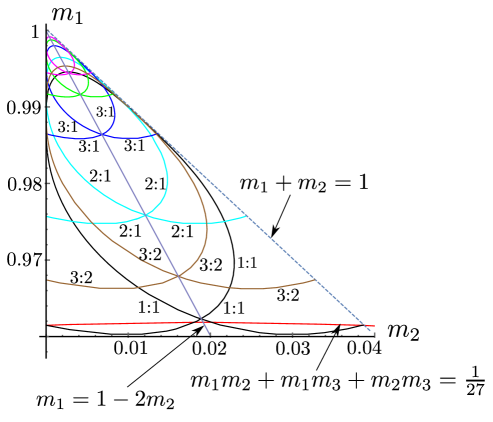
(a) Region III.

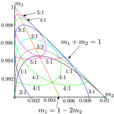
(b) The enlarged graph.

Figure 10. Resonance curves for equilibrium points $L_{3}$, $L_{5}$ and $L_{6}$ on the region III. The line is $m_{1}=1-2m_{2}$, that is, $m_{2}=m_{3}$.

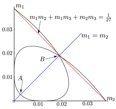
Figure 11. Resonance $1$:$1$ with two primary bodies with equal masses in the region II: $A(0.002736,0.002716)$ for $L_{5}$ and $B(0.01883,0.01883)$ for $L_{3}$ and $L_{6}$.

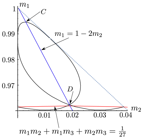
Figure 12. Resonance $1$:$1$ with two primary bodies with equal masses in the region III: $C(0.002736,0.994528)$ for $L_{3}$ and $D(0.01883,0.96234)$ for $L_{5}$ and $L_{6}$.

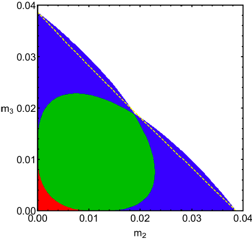
(a) The different colors indicate the total number of stable equilibrium points in region I. It is from [24].

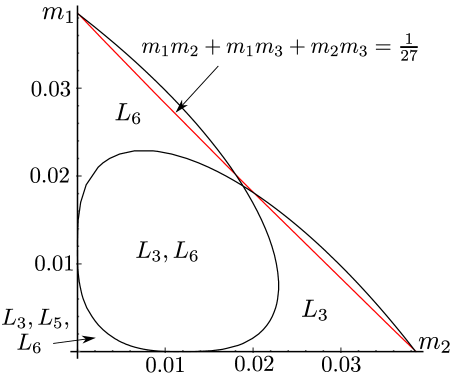
(b) Resonance $1$:$1$ curve on region I and the corresponding stable equilibrium points in the different areas.

Figure 13. (a) The different colors indicate the total number of stable equilibrium points in region I. (b) Resonance curves $1$:$1$ on region I and stability domain for $L_{3}$, $L_{5}$ and $L_{6}$. For some values of the masses the equilibrium points $L_{3}$ and $L_{6}$ are stable even though the Lagrange triangle is not.

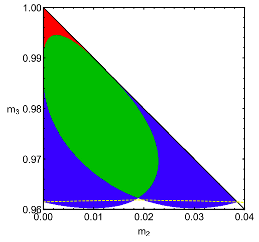
(a) The different colors indicate the total number of stable equilibrium points in region III. It is from [24].

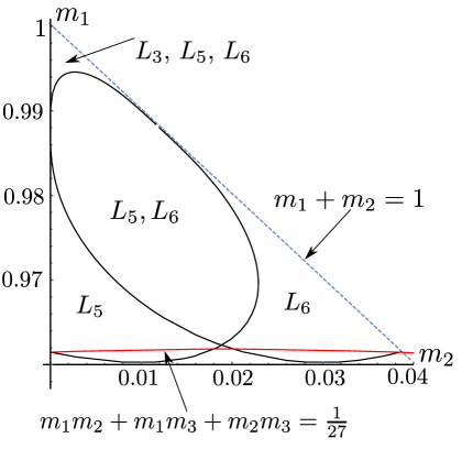
(b) Resonance $1$:$1$ curve on region III and the corresponding stable equilibrium points in the different areas.

Figure 14. (a) The different colors indicate the total number of stable equilibrium points in region III. (b) Resonance $1$:$1$ curve boundary of the stability region. For some vales of the masses the equilibrium points $L_{5}$ and $L_{6}$ are stable even though the Lagrange triangle is not.

Let us quickly mention the results recently reported by Bardin and Volkov [5]. They performed an analysis of stability and bifurcation of the equilibria in the ERFBP in the case that the Lagrangian triangular configuration of three bodies is stable. In particular, they show that the bifurcation is only possible in cases of degeneracy, when the mass of a primary body vanishes, that is, when the problem degenerates into two copies of the restricted three-body problem. Bardin and Volkov introduced the mass parameters $\mu_{2}=\frac{m_{2}}{m_{1}+m_{2}+m_{3}}$, $\mu_{3}=\frac{m_{3}}{m_{1}+m_{2}+m_{3}}$ and denoted by $P_{ij}$ the relative equilibrium that degenerates into a triangular libration point of the restricted three body problem $L_{i}^{(2)}$ as $\mu_{2}\to 0$, and degenerates into another triangular libration point $L_{j}^{(3)}$ as $\mu_{3}\to 0$. They claimed that $P_{45}$, $P_{54}$ and $P_{55}$ are the only points that can be both stable and unstable depending on values of parameters. The stability diagrams were constructed in the plane of parameters $\mu_{2}$ and $\mu_{3}$, and are shown in Figure 15. Hence, comparing the graphs in this figure with those in Figure 6(a) and Figure 7(a), we can conclude that their linear stability results are similar to ours, where $P_{45}\to L_{6}$, $P_{54}\to L_{3}$ and $P_{55}\to L_{5}$. It follows that the border between the stable and unstable regions computed by them are the resonance curves $1$:$1$.

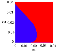
(a) Domains of stability of relative equilibria $P_{45}$

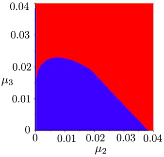
(b) Domains of stability of relative equilibria $P_{54}$

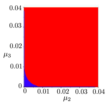
(c) Domains of stability of relative equilibria $P_{55}$

Figure 15. Graphs computed in [5], where instability domains are indicated by red color and domains of linear stability are indicated by blue color.

Now, we restrict our attention to the remarkable paper by Simó [22], where a detailed study is performed by analyzing numerically the relative equilibrium solutions in the four body problem. In particular, we point out in his Figure 7(a), where he displays the domain of linear stability of relative equilibria for the ERFBP in $1/6$ of the mass triangle, namely a half of region I from our Figure 2. To proceed in the analysis of his results, we note that the coordinates $(m_{2},m_{3})$ of the points marked in his plot are

$$A(\frac{1}{3},\frac{1}{3}),\quad B(0,\frac{1}{2}),\quad C(0,0),\quad S(0.0027096,0.0027096),\quad\;Y(0,0.038521),$$

$$T(0,0.011947),\;U(0.018858,0.018858),\;X(0.019034,0.019064),\;V(0.018114,0.020014).$$

His study was confined to the region where the three massive bodies configuration is stable, more precisely at $CYVX$ (see Figure 16). Simó shows that the region of stability is separated into three subregions given by $R_{4}=CST$, $R_{6}=CUT$, $R_{5}=CUVY$, such that $R_{4}\subset R_{6}\subset R_{5}$. By our calculations, we are able to identify the points marked by Simó on the boundary of the region $CYVX$, and what we get is shown in the Table 2 and displayed in Figure 16. We must remember that $m_{1}=m_{2}$ means that two primary bodies have equal masses.

The reader should note that the borders of the stability regions determined by Simó are just the resonance curves $1$:$1$, more precisely, $ST$ for $L_{5}$, $TU$ for $L_{6}$ and the arc $YVU$ for $L_{3}$. Futhermore, the regions $R_{4}\subset R_{6}\subset R_{5}$ are those shown in the Figures 13 and 14. For more details see Figure 16 where labels are shown.

point on border of $CYVX$	corresponds to
$U(0.018858,0.018858)$	point at $1$:$1$ resonance curves of $L_{3}$ and $L_{6}$ with line $m_{1}=m_{2}$:
	point $B$ in Figure 11
$V(0.018114,0.020014)$	intersection point between $1$:$1$ resonance curve of $L_{3}$
	and Routh’s critical curve: point $B_{L_{3}}$ in Figure 6 (a)
$T(0,0.011947)$	intersection point between $1$:$1$ resonance curve of $L_{5}$
	either $m_{1}=0$ or $m_{2}=0$: Figure 7 (a)
$S(0.0027096,0.0027096)$	point at $1$:$1$ resonance curve of $L_{5}$ with line $m_{1}=m_{2}$:
	point $A$ in Figure 11
$X(0.019034,0.019064)$	intersection point between the line $m_{1}=m_{2}$
	and Routh’s critical curve: Figure 8
$Y(0,0.038521)$	intersection point between the Routh’s critical curve and
	$1$:$1$ resonance curve of $L_{6}$ either $m_{1}=0$ or $m_{2}=0$:
	points $R_{L_{6}}$ and ${\mathcal{R}}_{L_{6}}$ in Figure 8

Table 2. Relationship between the values obtained by Simó those obtained by us.

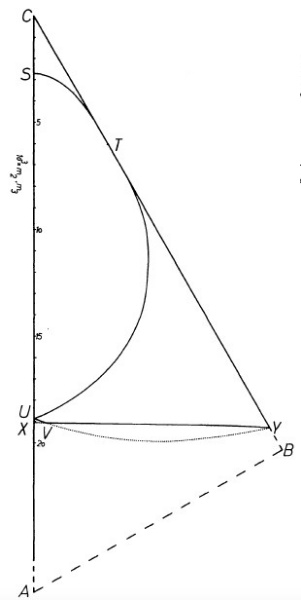
(a) It is Figure 7(a) taken from [22].

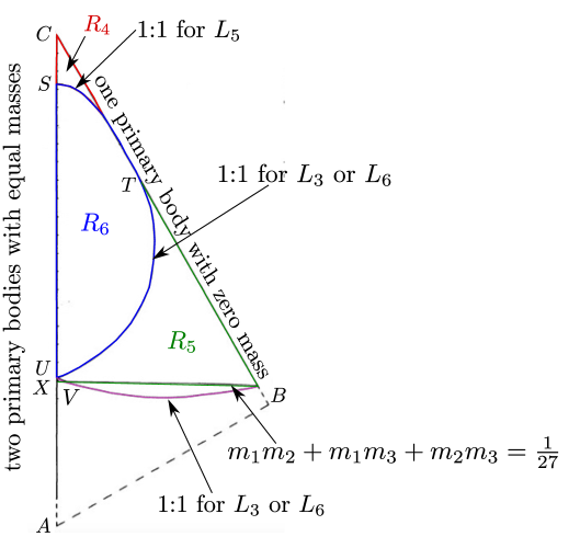
(b) Figure 7(a) with label on the curves and points obtained by [22].

Figure 16. The region $CYVX$ is the linear stability area of the primaries in the mass space, where $R_{4}=CST$, $R_{6}=CUT$ and $R_{5}=CUVY$ are stability regions of equilibrium points $L_{5}$, $L_{3}$ and $L_{6}$.

5. Concluding remarks

This paper summarizes the most known results (up to this date) about the location, counting and linear stability of the equilibrium points in the ERFBP.

In this review, the main attention was paid in the unification of known results about relative equilibria or central configuration of the planar restricted $(3+1)$-body problem with primaries in Lagrange’s configuration.

We would like to highlight that resonance curves are of utmost importance in determining the linear stability domain for the equilibrium points. Some resonance curves in region I were previously calculated by Budzko and Prokopenya, see [8] and [9]. However, we have given a step forward by computing some other resonance curves by taking into consideration the three regions in the plane where the Lagrange’s configuration turn out to be stable. This allowed us to determine regions, in a numerical way, in the mass space where the points of equilibrium are linearly stable, and to find out the regions where these points of equilibrium corresponds. Based on numerical methods, Zotos [24] showed the exact number of stable equilibrium points inside the regions I, II and III. In fact, he claims that regions where linearly stable points of equilibrium exist almost coincide with the regions for which the Lagrange’s configuration of the primaries is stable. We recall that similar results were reported by Budzco [8], but only for the equilibrium point $S_{1}$ ($L_{3}$ in our notation, see Table 1). Our analysis provide firm numerical evidence that $L_{3}$ and $L_{6}$ in region I, as well as $L_{5}$ and $L_{6}$ in regions II and III are stable in linear approximation for some mass values $m_{1}$, $m_{2}$ and $m_{3}$ which are outside the stability domain of the Lagrange’s triangle. Furthermore, we present numerical results to show that the boundaries of the stability domain are determined by the $1$:$1$ resonance curves. At present, this is a remarkable fact for which we have no explanation yet to offer. This is left, for now, as a future avenue of research on the ERFBP.

Statements and Declarations

The authors declare that they have no conflict of interest. This study was funded by the Universidad Autónoma Metropolitana (Metropolitan Autonomous University) Mexico.

José Alejandro Zepeda Ramírez and Martha Alvarez-Ramírez contributed to the design and implementation of the research, to the analysis of the results and to the writing of the manuscript.

Data sharing is not applicable to this article as no new data were created or analyzed in this study.

References

- [1] Alvarez-Ramírez, M., Vidal, C.: Math. Probl. Eng., Art. ID 181360, 23 pp. (2009).
- [2] Alvarez-Ramírez, M., Skea, J., T. Stuchi.: Astrophys. Space Sci. 358, 07 (2015). https://doi.org/10.1007/s10509-015-2333-4
- [3] Arenstorf, R. F.: Celestial Mech. 28, 9 (1982). https://doi.org/10.1007/BF01230655
- [4] Baltagiannis, A. N., Papadakis, K. E.: Internat. J. Bifur. Chaos Appl. Sci. Engrg. 21 (8), 2179 (2011). https://doi.org/10.1142/S0218127411029707
- [5] Bardin, B. S. and Volkov, E. V., 2021, in IOP Conf. Ser.: Mater. Sci. Eng., volume 012002, Springer, p. 1191
- [6] Barros, J. F., Leandro, E. S. G.: SIAM J. Math. Anal. 43 (2), 634 (2011). DOI: https://doi.org/10.1137/100789701
- [7] Barros, J. F., Leandro, E. S. G.: SIAM J. Math. Anal. 46 (2), 1185 (2014). https://doi.org/10.1137/130911342
- [8] Budzko, D.A., 2009, in Gadomski, L., et al. (eds.) Computer Algebra Systems in Teaching and Research. Evolution, Control and Stability of Dynamical Systems, The College of Finance and Management, Siedlce, p. 28
- [9] Budzko, D., Prokopenya, A., 2011, in E. W. Mayr V. P. Gerdt, W. Koepf and E. V. Vorozhtsov, editors, CASC 2011. LNCS, volume 6885, Springer, p. 88
- [10] Burgos-García, J., Delgado, J: Celestial Mech. Dynam. Astronom. 117 (2), 113 (2013). https://doi.org/10.1007/s10569-013-9498-3
- [11] Figueras, J. L., Tucker, W., Zgliczynski, P.: arXiv:2204.08812 [math.DS], 2022.
- [12] Gannaway, J. R., 1981, “Determination of all central configurations in the planar 4-body problem with one inferior mass", Thesis (Ph.D.)-Vanderbilt University.
- [13] Gaschea, M.: Compt. Rend., 16, 393 (1843)
- [14] Hampton, M., Moeckel, R.: Invent. Math. 163 (2), 289 (2006). DOI: https://doi.org/10.1007/s00222-005-0461-0
- [15] Kulevich, J. L., Roberts, G. E., Smith, C. J.: Qual. Theory Dyn. Syst. 8 (2), 357 (2009). https://doi.org/10.1007/s12346-010-0006-9
- [16] Leandro, E.S.G.: J. Differ. Equ. 226 (1), 323-351 (2006). DOI: https://doi.org/10.1016/j.jde.2005.10.015
- [17] Meyer, K. R., Offin, D. C., 2017, “Introduction to Hamiltonian dynamical systems and the -body problem", third edition, Springer: Berlin, Heidelberg, New York.
- [18] Moeckel, R., 2015: “Central configurations". In: Llibre, J., Moeckel, R. and Simó, C, Birkhäuser (eds.) Central Configurations, Periodic Orbits, and Hamiltonian Systems, Advanced Courses in Mathematics - CRM Barcelona, pp. 105–167. Birkhäuser/Springer, Basel.
- [19] Pedersen, P.: Danske Vid. Selsk. Mat.-Fys. Medd. 21 (6), 80 (1944)
- [20] Pedersen, P.: Danske Vid. Selsk. Mat.- Fys. Medd. 26 (16), 37 (1952)
- [21] Routh, E. J.: Proc. Lond. Math. Soc. 6, 86 (1874/75)
- [22] Simó, C.: Celestial Mech. 18 (2), 165 (1978). https://doi.org/10.1007/BF01228714
- [23] Zepeda Ramírez, J. A., Alvarez-Ramírez, M., García, A.: Internat. J. Bifur. Chaos Appl. Sci. Engrg. 31 (11), Paper No. 2130031, 15 (2021). https://doi.org/10.1142/S0218127421300317
- [24] Zotos, E. E.: Internat. J. Bifur. Chaos Appl. Sci. Engrg. 30 (10), Paper No. 2050155, 14 (2020). https://doi.org/10.1142/S0218127420501552