Blanco DECam Bulge Survey (BDBS) IV: Metallicity Distributions and Bulge Structure from 2.6 Million Red Clump Stars

Abstract

We present photometric metallicity measurements for a sample of 2.6 million bulge red clump stars extracted from the Blanco DECam Bulge Survey (BDBS). Similar to previous studies, we find that the bulge exhibits a strong vertical metallicity gradient, and that at least two peaks in the metallicity distribution functions appear at $b<-5^{\circ}$. We can discern a metal-poor ([Fe/H] $\sim$ $-0.3$) and metal-rich ([Fe/H] $\sim$ $+$0.2) abundance distribution that each show clear systematic trends with latitude, and may be best understood by changes in the bulge’s star formation/enrichment processes. Both groups exhibit asymmetric tails, and as a result we argue that the proximity of a star to either peak in [Fe/H] space is not necessarily an affirmation of group membership. The metal-poor peak shifts to lower [Fe/H] values at larger distances from the plane while the metal-rich tail truncates. Close to the plane, the metal-rich tail appears broader along the minor axis than in off-axis fields. We also posit that the bulge has two metal-poor populations – one that belongs to the metal-poor tail of the low latitude and predominantly metal-rich group, and another belonging to the metal-poor group that dominates in the outer bulge. We detect the X-shape structure in fields with |Z| $>$ 0.7 kpc and for stars with [Fe/H] $>$ $-0.5$. Stars with [Fe/H] $<$ $-0.5$ may form a spheroidal or “thick bar" distribution while those with [Fe/H] $\ga$ $-$0.1 are strongly concentrated near the plane.

1 Introduction

Bulge formation in massive disk galaxies is a complicated process that can involve a variety of physical mechanisms, such as: violent dissipative collapse (Eggen et al., 1962; Larson, 1974), merger events (Cole et al., 2000; Hopkins et al., 2009; Athanassoula et al., 2017), secular disk evolution (Combes et al., 1990; Kormendy & Kennicutt, 2004), clump coalescence (Elmegreen et al., 2008), and early gas-compaction (Dekel & Burkert, 2014; Zolotov et al., 2015; Tacchella et al., 2016). These processes, or some combination thereof, result in two broad classes of bulges: classical and pseudobulges (Kormendy & Kennicutt, 2004; Athanassoula, 2005; Fisher & Drory, 2016). However, some galaxies are known to harbor both components simultaneously (Peletier et al., 2007; Erwin et al., 2015, 2021).

Classical/merger-built bulges form violently and early in a galaxy’s history, and produce spheroidal, pressure-supported structures dominated by old stars that can also exhibit a metallicity gradient. Conversely, pseudobulges form over longer time scales, exhibit cylindrical rotation, have flatter and more elongated profiles, may contain a broad age dispersion, and can display a boxy/peanut X-shape structure when viewed at appropriate angles. Although the Milky Way bulge exhibits some classical bulge characteristics, such as the existence of a vertical metallicity gradient (e.g., Zoccali et al., 2008; Johnson et al., 2011; Gonzalez et al., 2011; Gonzalez et al., 2013; Zoccali et al., 2017; Rojas-Arriagada et al., 2020) and a predominantly old age (e.g., Ortolani et al., 1995; Zoccali et al., 2003; Clarkson et al., 2008; Valenti et al., 2013; Renzini et al., 2018; Surot et al., 2019; Sit & Ness, 2020), the clear signatures of cylindrical rotation (Howard et al., 2009; Kunder et al., 2012; Ness et al., 2013b; Zoccali et al., 2014) and an extended X-shape structure (McWilliam & Zoccali, 2010; Nataf et al., 2010; Saito et al., 2011; Gonzalez et al., 2015; Ness & Lang, 2016) are indicative of a dominant pseudobulge/bar.

Interestingly, the Milky Way bulge also exhibits strong evidence supporting a composite system. For example, stars with [Fe/H] $<$ $-$0.5 do not follow the same bar-like cylindrical rotation pattern observed in more metal-rich stars, and instead exhibit slow or null rotation and high velocity dispersion that are more reminiscent of a kinematically hot bar or spheroidal population (Soto et al., 2007; Babusiaux et al., 2010; Dékány et al., 2013; Ness et al., 2013b; Rojas-Arriagada et al., 2014; Kunder et al., 2016; Rojas-Arriagada et al., 2017; Zoccali et al., 2017; Clarkson et al., 2018; Arentsen et al., 2020; Kunder et al., 2020; Rojas-Arriagada et al., 2020; Wylie et al., 2021). Additional evidence supporting an accreted, rather than completely in situ, population is indicated by the existence of: at least two distinct RR Lyrae populations with different kinematic and pulsation period properties (Soszyński et al., 2014; Pietrukowicz et al., 2015; Kunder et al., 2019, 2020), N-rich (Schiavon et al., 2017; Horta et al., 2021; Kisku et al., 2021) and Na-rich (Lee et al., 2019) stars that are common in globular clusters but not in the field, and peculiar clusters such as Terzan 5 (Ferraro et al., 2009, 2016) and Liller 1 (Ferraro et al., 2021) that have large metallicity and/or age spreads. The latter clusters are posited to be remnant building blocks of the inner Galaxy; however, kinematic simulations suggest that any contribution to the total bulge mass by accretion/merger processes should be $<$ 8-10 per cent of the disk mass (Shen et al., 2010).

The composite nature of the Milky Way bulge/bar system is further confused by discrepancies in age measurements. Color-magnitude diagram (CMD) analyses almost universally find that bulge stars are $>$10 Gyr in age with a relatively small ($\sim$1-2 Gyr) age spread (Ortolani et al., 1995; Kuijken & Rich, 2002; Zoccali et al., 2003; Clarkson et al., 2008; Valenti et al., 2013; Gennaro et al., 2015; Renzini et al., 2018), and its RR Lyrae population may be among the oldest in the Galaxy (Savino et al., 2020). In contrast, several spectroscopic analyses (e.g., Bensby et al., 2013, 2017; Bovy et al., 2019; Hasselquist et al., 2020) have found that the bulge, particularly close to the plane, hosts a significant fraction of stars with ages $\sim$2-8 Gyr. Haywood et al. (2016) further claim that a degeneracy between age and metallicity could be masking the presence of young stars in previous CMD analyses, and that a substantial young population may be required to explain the relatively narrow main-sequence turn-off color spreads. However, the multi-color analysis by Renzini et al. (2018) argues against a significant ($>$ 5 per cent) population of young ($<$ 5 Gyr) stars in the bulge, even in relatively low latitude fields. Additionally, Barbuy et al. (2018) noted that the CMD simulation in Haywood et al. (2016) that included a prominent young population produced too many bright main-sequence turn-off stars and thus may be incompatible with observations. A similar discrepancy is seen in the possible discovery of young ($\sim$1 Gyr) blue loop stars in Baade’s Window by Saha et al. (2019), which are shown by Rich et al. (2020) to instead be nearby stars in the disk.

Uncertainty also surrounds the different metallicity distribution function interpretations and links between the bulge and thin/thick disk stars based on detailed chemical composition comparisons. Numerous sources find multiple “peaks" in the metallicity distribution functions that vary in amplitude as a function of Galactic latitude (e.g., Hill et al., 2011; Bensby et al., 2013; Ness et al., 2013a; Bensby et al., 2017; Zoccali et al., 2017; Duong et al., 2019a; Johnson et al., 2020; Rojas-Arriagada et al., 2020; Wylie et al., 2021), but both the number of populations fit and the [Fe/H] centroid locations of each group are inconsistent between papers. The discrepant results, coupled with significant differences in measurement methods and metallicity scales, complicate efforts to map the identified groups into known (e.g., thin/thick disk; halo) or newly defined (e.g., old classical bulge) populations.

Many papers speculate that the “metal-poor" and “metal-rich" peaks represent an inner extension of the thick and thin disks into the bulge/bar region (e.g., Ness et al., 2013a; Di Matteo et al., 2014, 2015; Debattista et al., 2017; Fragkoudi et al., 2018; Di Matteo et al., 2019). Such an assertion is supported by the similar detailed abundance patterns found in bulge stars and local thin/thick disk stars (e.g., Meléndez et al., 2008; Alves-Brito et al., 2010; Gonzalez et al., 2011; Jönsson et al., 2017; Zasowski et al., 2019). However, other surveys frequently find chemical evidence that especially the metal-poor bulge stars were enriched more quickly than the local disk (e.g., Zoccali et al., 2006; Fulbright et al., 2007; Johnson et al., 2011; Bensby et al., 2013; Johnson et al., 2014; Bensby et al., 2017; Rojas-Arriagada et al., 2017; Duong et al., 2019b).

Several of the issues outlined above result from the bulge’s complex geometric structure, strong differential reddening, high stellar density, significant foreground contamination, and large projection on the sky (e.g., Gonzalez et al., 2012, 2018). A variety of large-scale surveys, such as the Bulge Radial Velocity Assay (BRAVA; Rich et al., 2007a; Kunder et al., 2012), Vista Variables in the Via Lactea (VVV; Minniti et al., 2010), Gaia-ESO Survey (Gilmore et al., 2012), Abundances and Radial velocity Galactic Origins Survey (ARGOS; Freeman et al., 2013), GIRAFFE Inner Bulge Survey (GIBS; Zoccali et al., 2014), Apache Point Observatory Galactic Evolution Experiment (APOGEE; Majewski et al., 2017), HERMES Bulge Survey (HERBS; Duong et al., 2019a), and A2A survey (Wylie et al., 2021), have made significant progress in obtaining chemodynamic data in the bulge. However, the aforementioned problems have generally limited spectroscopic and/or photometric [Fe/H] measurements to $\sim$10⁴ total stars and often only $\sim$100-200 stars per field.

A new approach utilizing the $u-i$ color and the 3 square degree field-of-view of the Dark Energy Camera (DECam; Flaugher et al., 2015) was demonstrated by Johnson et al. (2020) to be an efficient method for measuring [Fe/H] in large samples of bulge red clump stars. The color-metallicity relation presented in Johnson et al. (2020) provides the framework for expanding the number of red clump stars with [Fe/H] measurements from thousands to millions. Therefore, in this paper we exploit the $\sim$250 million star $ugrizY$ catalog spanning $>$ 200 square degrees in the Southern Galactic bulge provided by the Blanco DECam Bulge Survey (BDBS; Rich et al., 2020; Johnson et al., 2020) to extract metallicity and distance estimates for $\sim$2.6 million red clump stars between $|l|<10^{\circ}$ and $-10^{\circ}<b<-3.5^{\circ}$.

2 BDBS Data Selection

Low mass stars with [Fe/H] $\ga$ $-1$ evolve off the red giant branch (RGB) after undergoing core He ignition and settle into the stable red clump evolutionary phase. Red clump stars are easily observed in the bulge (see Figure 1) and serve as standard candles for tracing the three dimensional structure of the inner Galaxy (e.g., Stanek et al., 1994; McWilliam & Zoccali, 2010; Nataf et al., 2010; Saito et al., 2011; Cao et al., 2013; Wegg & Gerhard, 2013; Simion et al., 2017; Gonzalez et al., 2018; Paterson et al., 2020). Although the red clump feature stands out as a clear over-density on the blue side of the RGB in Figure 1, isolating a pure bulge red clump sample can be challenging. This is particularly true for the BDBS catalog adopted here, which uses near-UV and optical filters, covers a large area, and includes hundreds of millions of stars.

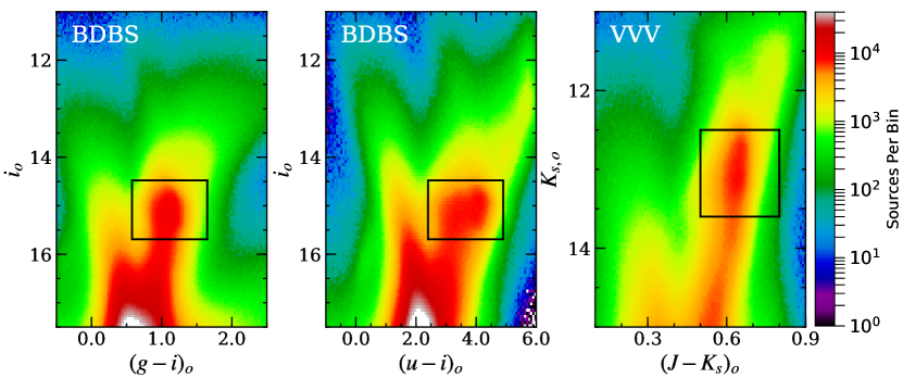
Figure 1: Density maps for dereddened CMDs from BDBS (left and middle panels) and VVV (right panel) are shown for fields with $|l|<10^{\circ}$ and $-10^{\circ}<b<-3.5^{\circ}$. The black boxes indicate the adopted red clump regions in each CMD. The blue plumes to the left of the black boxes are predominantly composed of foreground disk stars. Note that while the $i_{o}$ vs. $(g-i)_{o}$ and $K_{s,o}$ vs. $(J-K_{s})_{o}$ CMDs exhibit relatively narrow red clump color dispersions, the $i_{o}$ vs. $(u-i)_{o}$ red clump spans at least 2 mag. in color. The $(u-i)_{o}$ red clump spread is driven by metallicity variations, and highlights the utility of the $u$-band over redder filters in separating stars by heavy element composition.

Several effects conspire to add uncertainty in the red clump selection process, such as: differential reddening, distance variations, and foreground contamination along a line-of-sight. Differential reddening was addressed by employing the 1$\arcmin$ $\times$ 1$\arcmin$ reddening map described in Simion et al. (2017) and Johnson et al. (2020) to correct the observed $ugi$ photometry for all fields with $|l|<10^{\circ}$ and $-10^{\circ}<b<-3.5^{\circ}$. The BDBS footprint extends outside this selection box, but our reddening map currently only covers $l$ $\pm$ $10^{\circ}$ and $b>-10^{\circ}$. Fields interior to $b=-3.5^{\circ}$ are also omitted due to significantly higher extinction and stronger sub-arcminute reddening variations along most lines-of-sight.

For the dereddened $ugi$ BDBS CMDs utilized in this work, distance variations among red clump stars are manifested as a vertical spread in magnitude. Accounting for distance variations during the target selection process is particularly important because: (1) the bulge/bar system is oriented at an angle of $\sim$ 30^∘ and thus stars are distributed at distances exceeding $\pm$ 1 kpc from the Galactic Center, depending on the sight line; and (2) the bulge’s X-shape structure produces a double red clump along some sight lines, particularly those on the near-side of the bar with $b<-5^{\circ}$ (McWilliam & Zoccali, 2010; Nataf et al., 2010; Saito et al., 2011).

Foreground contamination is mostly observed as an overlap between the nearly vertical blue plume feature seen in Figure 1 and the blue edge of the bulge red clump. Although the bulge red clump and foreground blue plume features are well-separated along some sight lines, in other fields the distinction is more nebulous (see Figure 2). The variable separations between the red clump and foreground disk are largely driven by changes in the mean metallicity of bulge stars with Galactic latitude that are coupled with differences between foreground/bulge reddening along a particular line-of-sight (see also Section A).

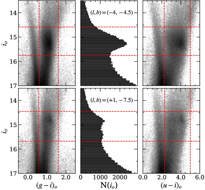
Figure 2: The left panels show $i_{o}$ vs. $(g-i)_{o}$ BDBS CMDs for 0.5^∘ $\times$ 0.5^∘ fields centered near $(l,b)$ = $(-4,-4.5)$ on the top and $(l,b)$ = $(+1,-7.5)$ on the bottom. The bulge red clump and foreground blue plume populations are obvious in both panels. The vertical and horizontal dashed red lines illustrate the magnitude and color limits for the red clump selection boxes in each field. The middle panels show $i_{o}$ luminosity functions for stars inside the selection boxes. The right panels show similar $i_{o}$ vs. $(u-i)_{o}$ CMDs with the dashed red lines indicating equivalent selection boxes. Note the increased color dispersion and complex morphology present when using the $u$-band, and the double red clump in the outer bulge field.

Given the large amount of data in the BDBS catalog, along with distance and contamination effects that need to be controlled, we determined the red clump selection boxes by visually inspecting $i_{o}$ vs. $(g-i)_{o}$ CMDs in 3 square degree regions across the aforementioned survey footprint (i.e., the sky grid boxes shown in Figure 5 of Johnson et al. 2020). For each field, the bright and faint $i_{o}$ limits were determined by inspecting the $i$-band luminosity function and designating where the star counts rose above the background RGB distribution. In fields where the double red clump was prominent, the bright and faint limits were set to encapsulate both populations.

Color cuts in each visual inspection field were determined purely from $(g-i)_{o}$. A constant red limit of $(g-i)_{o}$ = 1.6 was used for all fields. However, the blue color limit was set such that the visible portion of the blue plume did not overlap with the red clump at the faint $i_{o}$ limit.

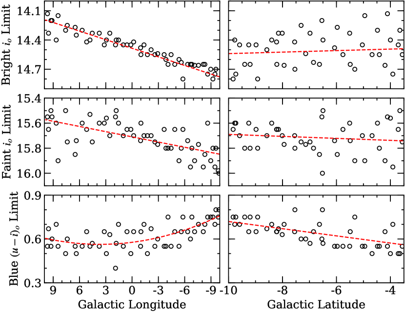
Figure 3: The top, middle, and bottom rows show the selection box limits for the bright $i_{o}$, faint $i_{o}$, and blue $(u-i)_{o}$ parameters, respectively, as measured for individual visually inspected fields (open circles). The left column shows the change in these parameters as a function of Galactic longitude while the right column shows the distribution with respect to Galactic latitude. The dashed red lines are low order polynomial fits to the data.

Since the 3 square degree selection fields are discrete and arbitrarily selected while the data are continuous, we fit low order polynomials to the selection box limits in order to obtain analytical cut-offs as functions of Galactic latitude and/or longitude. The data and fits are shown in Figure 3, and indicate that the bright, faint, and blue limits vary smoothly as a function of Galactic longitude. The bright and faint $i$-band limits showed significantly more scatter and lower sensitivity to Galactic latitude; however, the blue $(u-i)_{o}$ limit was somewhat sensitive to both Galactic latitude and longitude. For consistency, we calculated the selection box limits using the longitude-based ($l$) functional forms only, which are:

$$i_{o,bright}=-0.027l+14.477,$$ (1)

$$i_{o,faint}=-0.015l+15.692,$$ (2)

and

$$(u-i)_{o,blue}=0.0011l^{2}-0.0077l+0.577,$$ (3)

with typical uncertainties of about 0.05-0.10 magnitudes. A star’s initial selection as a potential bulge red clump member was therefore based solely on its Galactic longitude and the application of Equations 1-3 (along with the additional constraint of $(g-i)_{o}<1.6$). Additional examples of the color and magnitude limits for various fields, based on applying Equations 1-3, are described in Section A and Figures 21-22.

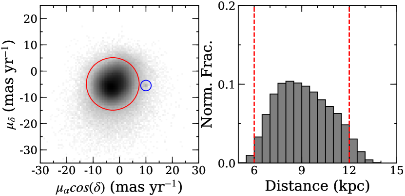
Figure 4: Left: a vector point proper motion diagram is shown for all potential red clump stars in our BDBS sample when matched to Gaia EDR3. The large red circle indicates the selection criteria used to separate likely bulge members from foreground field stars. The red circle has a radius of 9 mas yr^-1 ($\sim$ 1$\sigma$) and is centered at $\mu_{\alpha}$cos($\delta$) = $-$2.562 mas yr^-1 and $\mu_{\delta}$ = $-$5.376 mas yr^-1. The small clump observed to the right of the bulge population (blue circle) is the residual population of stars in the globular cluster M 22. Right: a histogram of red clump distances is shown for stars inside the red circle of the left panel. The peak of the distribution is approximately 8.2 kpc.

The number of stars initially identified as possible bulge red clump members exceeded 3 million. However, we culled this list further by removing targets with low quality measurements (large photometric errors, very high background values, unusual shape parameters, etc.) and those with radial distances within 5$\arcmin$ of all known globular clusters. The 5$\arcmin$ limit is sufficient to remove stars within $>$2-3 half-light radii of all clusters in our sample except M 22, which subtends a larger area on the sky. However, Figure 4 shows that M 22’s proper motion is outside our selection criteria for bulge field stars, and as a result we do not expect any significant contamination. Furthermore, we removed obvious foreground contamination using proper motions and parallaxes provided by the Gaia Early Data Release 3 catalog (EDR3; Gaia Collaboration et al., 2021). Figure 4 shows the results of matching our initial red clump catalog against EDR3. We only accepted stars inside the large red circle of Figure 4 that also had parallax values below 0.3 mas as bulge members.

The final step in cleaning the BDBS red clump sample utilized distance cuts to further constrain likely bulge members. Although red clump stars are reasonably stable standard candles, their $i$-band magnitudes are somewhat metallicity dependent. Numerous red clump absolute magnitude calibrations exist for a variety of bands (e.g., Alves, 2000; Girardi & Salaris, 2001; Laney et al., 2012; Hawkins et al., 2017; Ruiz-Dern et al., 2018; Onozato et al., 2019; Plevne et al., 2020), but these studies either do not include the metallicity dependence or are lacking a calibration for the BDBS bands. Therefore, we developed a metallicity dependent $i$-band calibration for stars with $-1<$ [Fe/H] $<+0.5$, based on Pan-STARRS system (Chambers et al., 2016) isochrones from the MESA Isochrones and Stellar Tracks database (MIST; Choi et al., 2016).

Briefly, we generated a set of 10 Gyr isochrones with 0.1 dex steps in [M/H] while assuming [$\alpha$/Fe] = $+$0.3 for [Fe/H] $<$ $-$0.3, [$\alpha$/Fe] = $-$[Fe/H] for $-0.3<$ [Fe/H] $<0.0$, and [$\alpha$/Fe] = 0.0 for [Fe/H] $>$ 0.0 (see also Joyce et al., 2022). For compatibility with the MIST database, we converted the [Fe/H] and [$\alpha$/Fe] values into [M/H] ratios via Equation 5 of Nataf et al. (2013):

$$[M/H]=[Fe/H]+log(0.638\cdot 10^{[\alpha/Fe]}+0.362).$$ (4)

We then fit a linear function through the red clump evolutionary point on each track where stars spend the most time and derived a relation between absolute dereddened $i$-band magnitude ($M_{i,o}$) and [M/H]:

$$M_{i,o}=0.266[M/H]+0.364,$$ (5)

or equivalently in [Fe/H] space with the adopted [$\alpha$/Fe] trends folded in:

$$M_{i,o}=0.199[Fe/H]+0.388.$$ (6)

Similarly, distances in kpc for each red clump star were calculated via the relation:

$$d=\frac{10\left[10^{\left(i_{o}-M_{i,o}\right)/5}\right]}{1000}.$$ (7)

The derived distance distribution is shown in the right panel of Figure 4 where we indicate the adopted bulge membership limits of 6 $<$ d $<$ 12 kpc. The distribution is slightly skewed toward the near end of the bar with a tail to the far end, but this is likely due to a combination of the proper motion cleaning preferentially removing foreground stars along with viewing angle effects. We note also that the distribution in Figure 4 peaks at a distance of $\sim$8.2 kpc, which is in good agreement with a recent geometric estimate of 8.178 kpc for the Galactic Center by Gravity Collaboration et al. (2019).

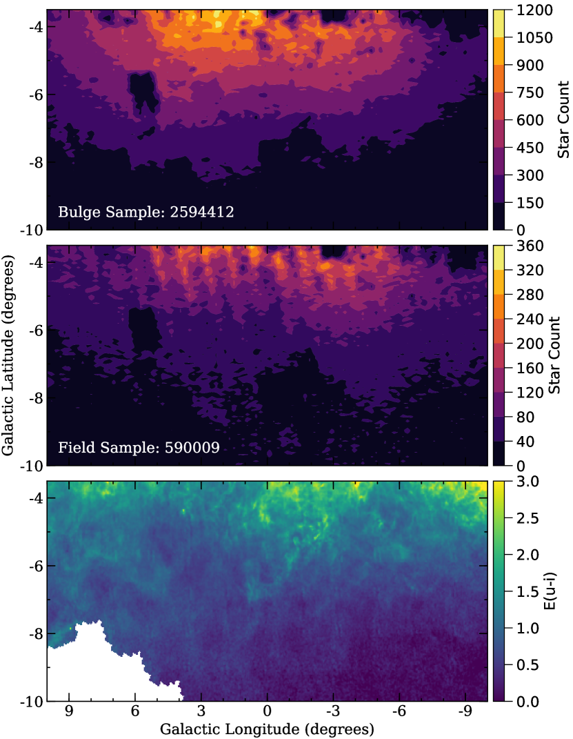
Figure 5: Star count contours are shown for our final catalog of likely bulge red clump stars (top panel) and those rejected as foreground contamination (middle panel). The small “holes" in the contours represent omitted regions due to the close proximity (5$\arcmin$) of known globular clusters. The few larger low-count regions are due to incomplete sampling in the BDBS data set. The regular, nearly vertical striping feature, seen especially at positive longitudes in the field sample and close to the plane, is due to the Gaia scanning function. The bottom panel shows the E($u-i$) reddening adopted for this work.

Figure 5 shows the spatial distribution of red clump stars in our final catalog, along with an E($u-i$) reddening map derived from Simion et al. (2017). The catalog reproduces the expected shape of the bulge/bar system, and except for a few low count regions due to incomplete sampling, such as near $(l,b)=(+6^{\circ},-6^{\circ})$, the star counts smoothly vary across the BDBS footprint. The final catalog includes $\sim$2.6 million likely red clump bulge members while $\sim$600,000 were rejected as likely foreground stars. A list of coordinates (corrected for spatial detector distortions; Clarkson et al., in prep.), $ugi$ photometry, A_λ, [Fe/H], distance values, and associated errors is provided in Table 1.

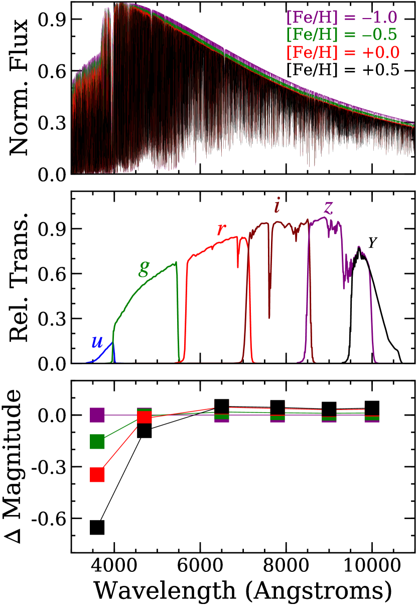
Figure 6: Top: synthetic high resolution spectra from the POLLUX database (Palacios et al., 2010) are shown for typical red clump stars (T_eff = 5000 K, log(g) = 2.5 cgs) spanning $-1<$ [Fe/H] $<+0.5$. Stars with [Fe/H] $<$ 0 were modeled with [$\alpha$/Fe] = $+$0.4 while higher metallicity stars had [$\alpha$/Fe] = 0. Note that the spectra are normalized to each have the same peak flux. Middle: filter response curves for the DECam filters used in BDBS. Bottom: each box shows the difference in magnitude for a given filter between the [Fe/H] = $-$1 spectrum (purple) and those with [Fe/H] = $-$0.5 (green), $+$0.0 (red), and $+$0.5 (black). The magnitude differences were calculated by convolving the filter response curves with the original, non-normalized spectra in the top panel.

3 Red Clump [Fe/H] Measurements from $u$-band Photometry

3.1 Red Clump Color-Metallicity Relation

Near-UV photometry has been used for decades to measure the metallicities of stars across a variety of evolutionary states and populations (e.g., Eggen et al., 1962; Keller et al., 2007; Ivezić et al., 2008; Zou et al., 2016; Ibata et al., 2017; Howes et al., 2019; Mohammed et al., 2019; Nataf et al., 2021). Figure 6 highlights the advantage of the $u$-band over redder filters when separating red clump stars based on their metallicities. The $u$-band appears to remain sensitive to changes in metallicity up to very high values. Even for [Fe/H] = $+$0.5, the cumulative absorption effects of many weaker metal lines blueward of $\sim$4000 Å can be seen despite the growing saturation of stronger features. This explains the large red clump color dispersions seen in Figures 1-2 when the $u$-band is included, compared to those with redder bands.

The effects illustrated in Figure 6 were exploited by Johnson et al. (2020) and Lim et al. (2021a) to show that the $(u-g)_{o}$ and $(u-i)_{o}$ colors of BDBS red clump stars are well-correlated with spectroscopic [Fe/H] measurements over the full metallicity range of typical bulge stars. For this work, we employed the color-metallicity relation given by Equation 22 of Johnson et al. (2020):

$$[Fe/H]=0.563(u-i)_{o}-2.074,$$ (8)

which is calibrated with overlapping stars in the GIBS database (Zoccali et al., 2017). As mentioned previously, the $u$ and $i$-band photometry, extinction coefficients, [Fe/H] values, and associated errors are provided in Table 1.

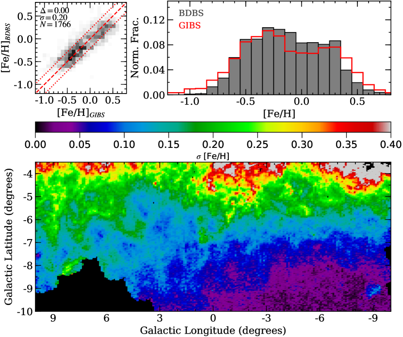
Figure 7: Left: a density map comparing the photometric (BDBS) and spectroscopic (GIBS) [Fe/H] values is shown. The dashed red line shows the fit from Equation 8 while the dotted red lines show the measured 0.2 dex dispersion. Note that the dispersion value was calculated after a single sigma-clipping pass to remove extreme ($>$ 3$\sigma$) outliers. The comparison includes $>$ 1700 stars in common between BDBS and GIBS, and spans all GIBS fields that overlap with Table 1. Right: The grey (BDBS) and red (GIBS) histograms illustrate the derived metallicity distribution functions using all stars shown in the left panels. Both distributions are similarly broad and appear bimodal. Bottom: an [Fe/H] uncertainty map, based on the errors provided in Table 1, is shown. Since the $u$-band photometric and reddening errors dominate the [Fe/H] uncertainty, this map is morphologically similar to the E($u-i$) panel of Figure 5.

The $u$-band photometric and reddening uncertainties are expected to dominate the [Fe/H] error budget, along with associated uncertainties in the transformations between the original VISTA-based extinction map and our adopted SDSS and Pan-STARRS calibration systems (see Section 3.4 of Johnson et al., 2020). The [Fe/H] uncertainty values from Table 1 are calculated via error propagation of Equation 8:

$$\begin{split}\sigma_{[Fe/H]}=\Bigl{[}\left(\frac{\partial[Fe/H]}{\partial u}\sigma_{u}\right)^{2}+\left(\frac{\partial[Fe/H]}{\partial A_{u}}\sigma_{A_{u}}\right)^{2}+\\ \left(\frac{\partial[Fe/H]}{\partial i}\sigma_{i}\right)^{2}+\left(\frac{\partial[Fe/H]}{\partial A_{i}}\sigma_{A_{i}}\right)^{2}\Bigr{]}^{\frac{1}{2}},\end{split}$$ (9)

where $\sigma_{u}$ and $\sigma_{i}$ are the photometric errors from Table 1 and $\sigma_{A_{u}}$ and $\sigma_{A_{i}}$ are derived from the E($J-K_{S}$) uncertainty values in the VVV map propagated with Equations 14, 15, 16, and 19 of Johnson et al. (2020). We find a median [Fe/H] uncertainty of 0.19 dex, but the bottom panel of Figure 7 shows that the typical uncertainty value is correlated with Galactic latitude. Fields with $b<-6^{\circ}$ generally have $\sigma_{[Fe/H]}$ $<$ 0.15 dex while those closer to the plane have uncertainties closer to 0.2-0.3 dex, due to the increased crowding and extinction.

However, the top panels of Figure 7 indicate that the BDBS-GIBS calibration is relatively uniform across a variety of sight lines, with a 1$\sigma$ scatter of 0.2 dex. We note that Lim et al. (2021a, see their Figure 8) found an almost identical calibration and dispersion when comparing BDBS photometric [Fe/H] values against a separate spectroscopic metallicity scale published in Lim et al. (2021b).

Johnson et al. (2020, see their Figures 18-19) also showed from comparisons with red clump stars in globular clusters that typical BDBS [Fe/H] uncertainties, even in very crowded fields, can be as low as $\sim$0.10-0.15 dex across a wide range of metallicities. The top right panel of Figure 7 also indicates that the BDBS-derived metallicity distribution functions are generally well-matched against those from GIBS.

Finally, distance uncertainties in Table 1 are calculated from standard error propagation of Equations 6 and 7:

$$\sigma_{d}=\sqrt{\left(\frac{\partial d}{\partial i}\sigma_{i}\right)^{2}+\left(\frac{\partial d}{\partial A_{i}}\sigma_{A_{i}}\right)^{2}+\left(\frac{\partial d}{\partial M_{i,o}}\sigma_{M_{i,o}}\right)^{2}},$$ (10)

where the $\sigma_{i}$ and $\sigma_{A_{i}}$ values are the same as those in Equation 9. The $\sigma_{M_{i,o}}$ term is calculated from:

$$\sigma_{M_{i,o}}=\sqrt{\left(\frac{\partial M_{i,o}}{\partial[Fe/H]}\sigma_{[Fe/H]}\right)^{2}+\sigma_{M_{i,o;RC}}^{2}},$$ (11)

where the $\sigma_{[Fe/H]}$ value is taken from Equation 9 and $\sigma_{M_{i,o;RC}}$ is set to 0.1 mag. in order to roughly account for the luminosity uncertainty of the red clump phase.

3.2 Contamination and Biases

Despite our efforts described in Section 2 to isolate a clean bulge red clump sample, first ascent RGB overlap and inner disk contamination are inevitably still present in the final sample. Additionally, a variety of observational biases exist when observing red clump stars that can skew results (e.g., see the discussion in Nataf et al., 2014). Among these issues are age variations (Bensby et al., 2013, 2017; Bovy et al., 2019; Saha et al., 2019; Hasselquist et al., 2020), metal-poor selection effects (e.g., Nataf et al., 2014), and [$\alpha$/Fe] trends (i.e., whether the bulge [$\alpha$/Fe] ratio flattens out at [Fe/H] $>$ 0 or continues to decrease).

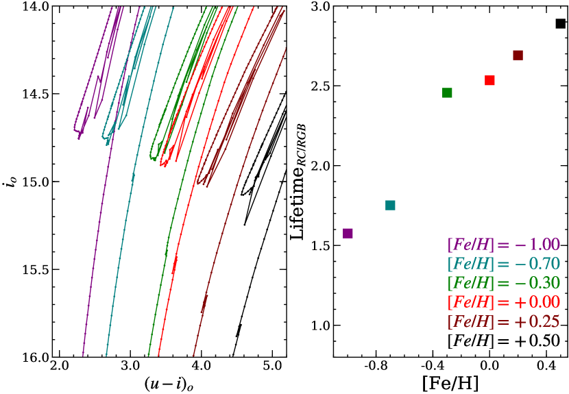
Figure 8: Left: 10 Gyr MIST isochrones are shown for [Fe/H] values ranging from $-1$ to $+$0.5, and for which [$\alpha$/Fe] linearly decreases from $+$0.3 to $+$0.0 between $-0.3<$ [Fe/H] $<+0.0$. The [$\alpha$/Fe] ratios are assumed constant on either side of the [Fe/H] cut-off. For display purposes, the isochrones have been shifted to a distance of 8 kpc. Right: the relative lifetime ratios of stars passing through RGB and red clump phases within a typical BDBS selection box are plotted as filled squares for each track. The RC/RGB lifetime ratio is a rough tracer of the expected contamination rate for first ascent RGB stars passing through the BDBS selection box.

The bulge exhibits a wide range of [Fe/H] values along all sight lines, and as a result first ascent RGB stars will overlap with almost any selection criteria used to extract red clump stars. This effect is clearly seen in the left panel of Figure 8, which generally covers our red clump selection region and shows that red clump and RGB stars overlap the same CMD space. The bar angle depth of $\sim$ $\pm$ 2 kpc also adds an additional mixing of evolutionary states. However, the right panel of Figure 8 shows that legitimate red clump stars still dominate the number density in this region by a factor of 1.5-3.0, depending on the metallicity. Since most bulge stars have [Fe/H] $>$ $-0.5$, we can reasonably expect that $\sim$70 per cent of the targets in our selection boxes are true red clump stars.

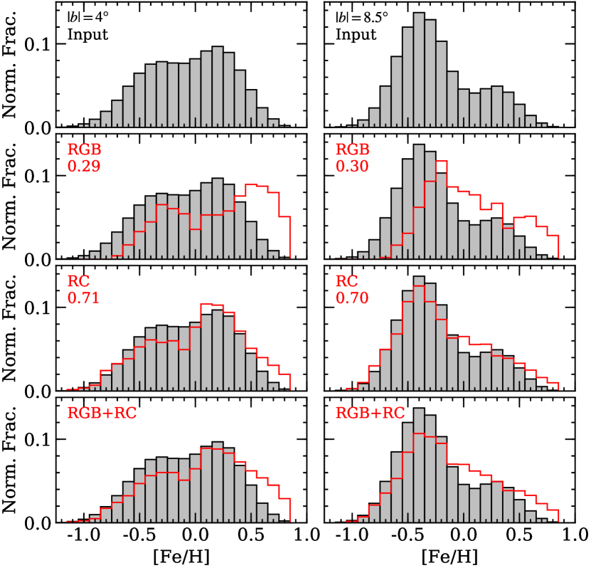
Figure 9: Top row: input metallicity distribution functions generated from the two-component Gaussian profile fits of Zoccali et al. (2017) for fields with $|b|=4^{\circ}$ (inner bulge) and $|b|=8.5^{\circ}$ (outer bulge). These functions are used to test the impact of RGB contamination when deriving metallicity distributions from CMD regions dominated by the red clump. Second row: the open red histograms illustrate the photometric metallicity distribution functions of RGB stars in each field if the red clump color-metallicity relation from Equation 8 is applied. The numbers in each panel are the fractional contributions to expected star counts in our adopted red clump selection box. The grey histograms are the original input metallicity distributions from the top row. Third row: similar to the previous row but for red clump stars. Bottom row: the combined photometric metallicity distribution functions of each field weighted by the expected RC/RGB ratios.

We illustrate in Figure 9 the impact on our derived metallicity distribution functions when accounting for a mixing of red clump stars with those on the RGB. The top panels illustrate sample metallicity distributions for inner and outer bulge fields constructed from the analytical fits given in Zoccali et al. (2017). Although the Zoccali et al. (2017) sample suffers from many of the same issues noted above, for simplicity we will assume that these spectroscopic abundances reflect the true underlying distributions along the sight lines. We generated a fine grid ($\Delta$[Fe/H] = 0.01) of isochrones by interpolating/extrapolating among the tracks shown in Figure 8 to construct a mock CMD that reflects the expected metallicity distributions. Stars were placed on the isochrone grid using the duration of the evolutionary phase that each point occupies as a weight. The middle panels reflect the derived metallicity distribution functions of RGB and red clump stars assuming both sets had their $(u-i)_{o}$ colors converted to [Fe/H] using Equation 8 (i.e., assuming they are all red clump stars).

The middle panels of Figure 9 show that while the red clump sample generally does a reasonable job of recreating the input metallicity distribution, the RGB-based distribution is predictably shifted towards higher [Fe/H]. The RGB stars also produce an unrealistic metal-rich tail. However, the combined distributions in the bottom panels, which reflect the procedure used in this paper, are morphologically similar to the original input distributions. The primary effects of combining RGB and red clump stars appears to be a reduction in the metal-poor tail, an enhancement in the metal-rich tail, and a slight change to the “gap" distance between the metal-poor and metal-rich peaks.

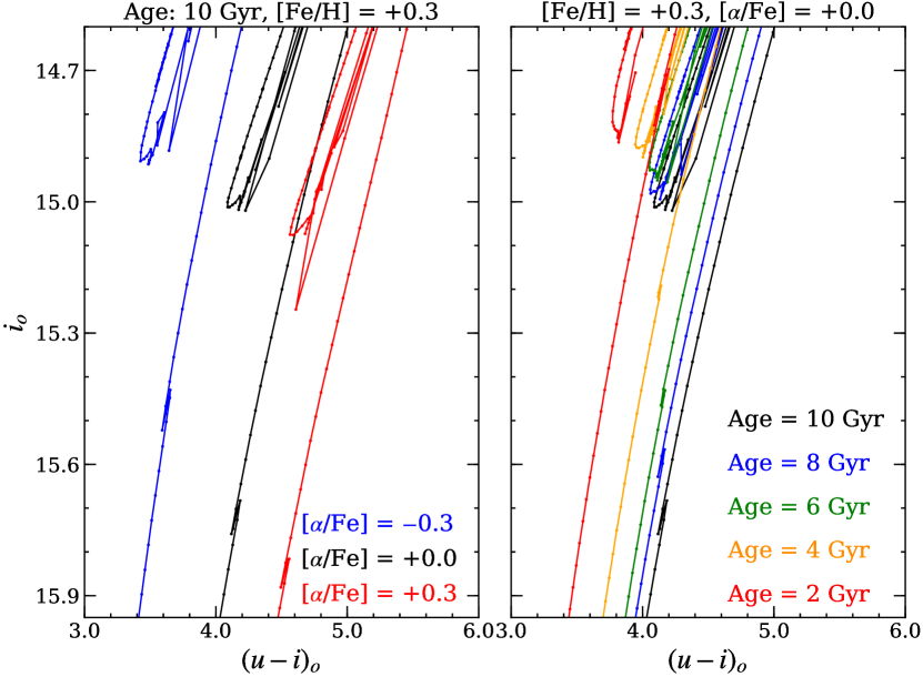
Figure 10: The left panel illustrates the isochrone effects of changing the [$\alpha$/Fe] composition by $\pm$ 0.3 dex for a 10 Gyr old, metal-rich population. Note that decreasing the [$\alpha$/Fe] composition from 0.0 to $-$0.3 shifts the red clump $(u-i)_{o}$ distribution blueward by $\sim$0.3-0.4 mag. The right panel shows how age variations can affect the red clump location for a typical high metallicity bulge star. The red clump color distribution appears to be mostly insensitive to age variations as long as stars are older than $\sim$2-4 Gyr.

Age and [$\alpha$/Fe] variations can also affect the $(u-i)_{o}$ distribution and thus the derived [Fe/H] values. Although these variations are likely already folded into the empirical color-metallicity relation, it is instructive to examine how each could affect the derived metallicity distribution functions. We highlight two scenarios in Figure 10 where these effects may manifest.

The left panel of Figure 10 shows the impact on an [Fe/H] = $+$0.3, 10 Gyr evolutionary track induced by changing [$\alpha$/Fe] $\pm$ 0.3 dex from the expected Solar ratio. Since modifying [$\alpha$/Fe] while holding [Fe/H] constant is equivalent to changing [M/H], the isochrones move in the expected direction (i.e., higher metallicity stars are redder). This is potentially relevant to the bulge because: (1) not all $\alpha$-elements change in the same way with [Fe/H] (e.g., Fulbright et al., 2007; Gonzalez et al., 2011; Johnson et al., 2014); and (2) some data show [$\alpha$/Fe] leveling off at [Fe/H] $>$ 0 while others find that it continues to decrease with increasing metallicity (e.g., see Figure 6 of Barbuy et al., 2018, and references therein). However, for the bulge stars where this impact would be maximized ([Fe/H] $\ga$ +0.2), Figure 10 suggests that a 0.3 dex uncertainty in [$\alpha$/Fe] would only change the measured photometric [Fe/H] by $\sim$0.1-0.2 dex. Fortunately, no investigations have found compelling evidence that the mean [$\alpha$/Fe] trends differ significantly between fields.

Effects on the photometric metallicity values due to age variations are more concerning. While likely limited to stars with [Fe/H] $\ga$ 0, some evidence suggests that the prominence of young stars may be a strong function of the bulge/bar location being probed (e.g., Ness et al., 2014; Hasselquist et al., 2020). Although Bensby et al. (2013, 2017) find evidence supporting the existence of bulge stars as young as $\sim$2-3 Gyr, the general consensus is that stars significantly younger than 10 Gyr are probably found very close to the plane (e.g., Ness et al., 2014; Hasselquist et al., 2020). The right panel of Figure 10 shows that even if a young population exists in our fields these stars will not change the red clump color distribution in any significant way, as long as most stars are older than $\sim$2-4 Gyr. This assumption is further supported by recent analyses from Marchetti et al. (2022) and Joyce et al. (2022), which do not find evidence supporting a significant population of stars with ages below approximately 6 Gyr.

Finally, we note that disk and halo contamination rates for most bulge fields should be relatively small. For example, Zoccali et al. (2008) used the Besancon Milky Way model (Robin et al., 2003) to calculate that the thin disk, thick disk, and halo likely only contribute about 3, 6, and 0.1 per cent of all stars in the red clump region of Baade’s window. Although the disk fractions can increase to 10 per cent or more outside $b=-6^{\circ}$, we regard these as upper limits since our proper motion cleaning procedure likely removed a substantial number of foreground stars. We further note that because post-RGB stars with [Fe/H] $<$ $-1$ tend to reside on the blue horizontal branch rather than the red clump, our sample is inherently biased against the most metal-poor stars in the bulge. However, while dedicated searches have uncovered many metal-poor stars in the bulge (e.g., Walker & Terndrup, 1991; García Pérez et al., 2013; Howes et al., 2014, 2016; Arentsen et al., 2020; Savino et al., 2020; Lucey et al., 2021), surveys targeting the RGB, rather than just the red clump (e.g., Fulbright et al., 2006; Zoccali et al., 2008; Johnson et al., 2011; Johnson et al., 2013; Rojas-Arriagada et al., 2020), still find that stars with [Fe/H] $<$ $-1$ contribute only a small fraction ($\la$ 5 per cent) to the total bulge population.

4 Results and Discussion

4.1 BDBS Metallicity Distribution Functions

Numerous surveys have obtained high resolution spectroscopic [Fe/H] abundances for hundreds to thousands of bulge dwarf, red clump, and/or RGB stars (e.g., see Section 3.2.1 of Barbuy et al., 2018, and references therein) and discovered several persistent trends. All surveys find that most bulge stars are between $-1.0<$ [Fe/H] $<+0.5$, and that the metallicity dispersion is large ($\sigma_{[Fe/H]}>0.3$). A strong vertical metallicity gradient is universally observed with the bulge becoming more metal-poor at larger distances from the plane. Additionally, most studies find at least two peaks in the metallicity distribution functions that are often separated by $>$ 0.3 dex in [Fe/H], and that the amplitudes of the metal-poor and metal-rich peaks vary with Galactic latitude. The metallicity distributions are often decomposed into two or more populations using Gaussian Mixture Model methods.

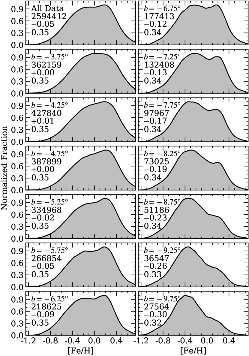
Figure 11: The top left panel shows the metallicity distribution function of all likely bulge red clump stars included in Table 1. Similarly, the remaining panels show the red clump metallicity distribution functions summed across all longitudes, using vertical strips spanning $\pm$ 0.25^∘ in latitude. The number of stars, center stripe positions, mean [Fe/H], and $\sigma_{[Fe/H]}$ values are included for all panels. Note the strong change in distribution morphology as a function of Galactic latitude. Most fields clearly show two distribution peaks.

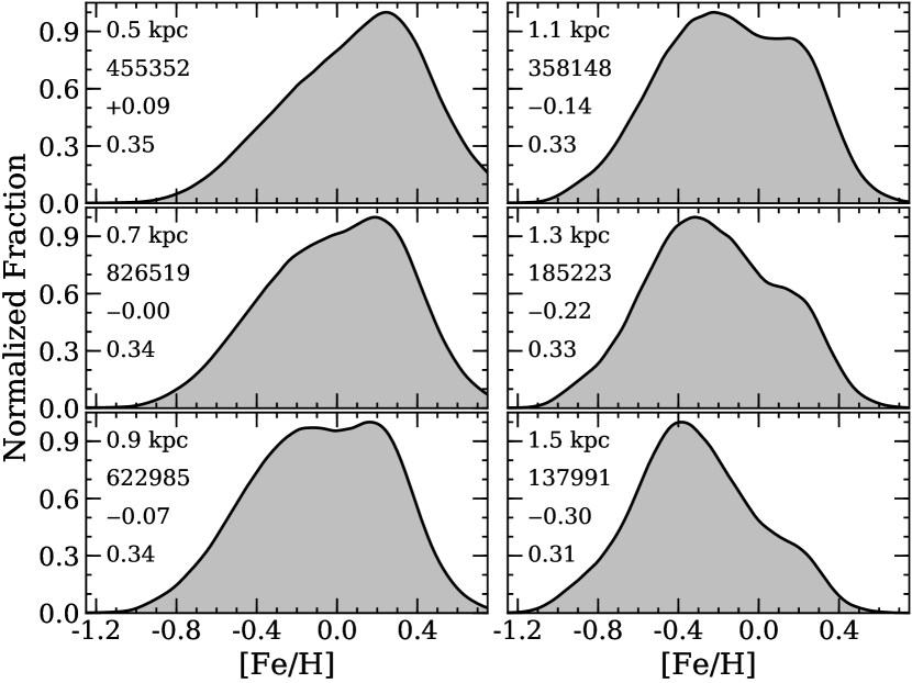
Figure 12: Similar to Figure 11, red clump metallicity distribution functions are shown as functions of distance from the Galactic plane (|Z|). Each slice encompasses all longitudes but only includes Z distances $\pm$ 0.1 kpc from the values given in each panel. The results are qualitatively in agreement with those of Figure 11 but the various peaks are sharper.

Despite these advances, several important questions remain unanswered:

• How is the metallicity gradient manifested? Is it simply the mixture of two populations with different mean [Fe/H] values that vary in scale height, or are vertical gradients intrinsic to one or more of these populations?

• Should the bulge instead be viewed as a “continuum" rather than a combination of discrete populations?

• Is the bulge distinct from the disk, or is it well-described as a composite of the thin and thick disks?

• If adopting a multi-component model for the bulge, are Gaussian distributions physically motivated or meaningful? This is especially important because authors often disagree on the number of components present, even in the same fields with largely overlapping samples, along with the individual fit widths, centroids, and amplitudes.

• Do the distribution tails hold any information about the bulge formation process?

Therefore, we add here new metallicity distribution functions for all 2.6 million red clump stars listed in Table 1. The BDBS data set is at least 100-1000$\times$ larger than previous spectroscopic surveys, and includes nearly uniform coverage between $|l|<10^{\circ}$ and $-10^{\circ}<b<-3.5^{\circ}$. Broad summaries of the data are provided in Figures 11-13 as summed distributions across all available longitudes in 0.5^∘ latitude and 0.2 kpc slices, respectively. We outline below several key observations related to changes in the distribution morphology, including: peak locations, gradients, and tails.

4.1.1 Metallicity Distribution Function Morphology

Visual inspection of Figures 11-13 shows that while all of the slices contain very broad distributions, the morphological shapes are strongly correlated with distance from the Galactic plane. The fields closest to the plane ($b>-5^{\circ}$ and |Z| $<$ 0.6 kpc) are strongly skewed to peak near [Fe/H] $\sim$ $+$0.2, and in some cases may be unimodal. Comparing the $b=-4.25^{\circ}$ and |Z| = 0.5 kpc panels of Figures 11-13 highlights that switching between observed ($b$) and physical (Z) coordinates modifies the distribution shapes. For example, the |Z| = 0.5 kpc panel of Figure 12 shows a more unimodal distribution and narrower metal-rich peak than the $b=-4.25^{\circ}$ panel of Figure 11, despite a significant overlap in stars. The reduced metal-poor peak when working in physical coordinates is likely driven by a removal of stars that lie along the same projected sight line in latitude but that are at farther distances, and thus larger |Z|, where the mean metallicity is lower.

The |Z| = 0.5 kpc distributions in Figure 13 are morphologically similar to the closed-box enrichment models described in earlier bulge work (e.g., Rich, 1990). The exception appears to be the fields located close to the plane but on the far side of the bar ($-6^{\circ}>l>-10^{\circ}$). Figure 13 shows that these fields are skewed toward a lower mean metallicity, and also exhibit a paucity of metal-rich stars when compared against similar sight lines on the near side and minor axis of the bulge. A similar behavior was noted by Zoccali et al. (2017) in their ($-8^{\circ},-6^{\circ}$) field, but they did not find any clear explanation for this discrepancy.

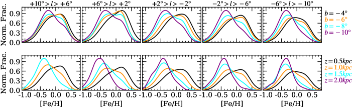
Figure 13: The top row shows metallicity distribution functions across 5 sight lines, each spanning 4 degrees in longitude. The black, orange, cyan, and purple lines show the metallicity distributions for two degree increments in latitude ranging from $b=-4^{\circ}$ to $-10^{\circ}$. The data are normalized such that the peak in the coordinate slice containing the most stars equals unity. The bottom panels show similar slices except the data are separated by vertical distance from the plane (|Z|). The data cover 0.5 kpc slices ranging from 0.5-2.0 kpc. Note that the left panel does not have a 2 kpc distribution because observing these stars on the near side of the bar would require observing at $b<-10^{\circ}$.

The remaining fields with |Z| < 1.5 kpc clearly show two peaks centered near [Fe/H] $\sim$ $-0.3$ and $+$0.2, but similar to previous work we find that the amplitudes change substantially when moving away from the plane. Fields interior to $b\sim-6^{\circ}$ and |Z| $\sim$ 0.8 kpc are skewed such that the global maxima are at the metal-rich peaks. For a narrow strip near $b=-6.5^{\circ}$ and |Z| = 1 kpc, the two peaks are equivalent in amplitude. Increasing the distance from the plane further leads to a rapid decline in the amplitude of the metal-rich local maxima.

The metallicity distributions in the outer fields ($b<-8.5^{\circ}$ and |Z| $>$ 1.5 kpc) are dominated by a broad, metal-poor population. However, despite the rapid decrease in amplitude of the metal-rich peak, it is still detectable in all fields with |Z| $<$ 1.75 kpc. The bottom panels of Figure 13 show that the outermost fields in our survey (|Z| $\sim$ 2 kpc) do not exhibit a clear metal-rich peak, and instead several of the fields have a secondary, more metal-poor peak near [Fe/H] $\sim$ $-0.8$. This population is likely related to the “C" group identified in Ness et al. (2013a) as the inner thick disk. We note that while the metallicity distribution changes substantially over a $\sim$ 1.5 kpc vertical slice of the bulge, the [Fe/H] dispersion remains nearly constant with $\sigma_{[Fe/H]}\sim 0.35$.

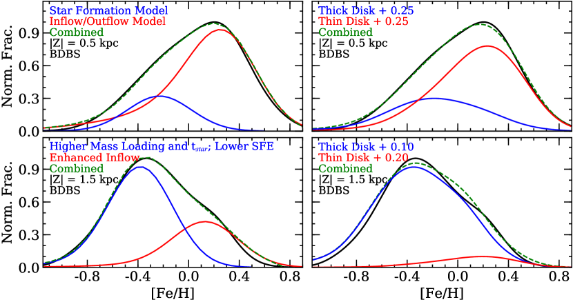
Figure 14: The top and bottom rows show the observed BDBS metallicity distribution functions (solid black lines) for bulge stars with 0.3 $<$ |Z| $<$ 0.7 kpc and 1.2 $<$ |Z| $<$ 1.8 kpc, respectively. The left panels compare the observed distributions against two analytical chemical enrichment models generated with the One-zone Model for the Evolution of GAlaxies (OMEGA) code (Côté et al., 2017). For both left panels, the blue and red lines represent the “star formation" and “inflow/outflow" OMEGA models that roughly correspond to the metal-poor and metal-rich components from Grieco et al. (2012). The sum of the two distributions are shown as dashed green lines, and all model outputs have been broadened by 0.25 dex to account for observational uncertainty. Compared to the top left models, the bottom left star formation model has an enhanced mass loading factor, a longer star formation time scale (t_star), and a lower star formation efficiency (SFE) to reduce the mean yield and broaden the metal-poor tail. Similarly, the inflow/outflow model has enhanced inflow of metal-poor gas to reduce the metal-rich tail. The right panels compare the BDBS distributions against the empirical thick (red) and thin (blue) disk distributions provided by Bensby et al. (2014). Both disk populations have been shifted upward by 0.10-0.25 dex to better align with the observed distribution peaks. The thin and thick disk distributions have also been broadened by 0.20 dex.

4.1.2 Metallicity Distribution Models

Examining the most interior and exterior fields of Figures 12-13, which should be dominated by the distributions that produce the metal-poor and metal-rich peaks, indicates that neither is likely well-described by a simple convolution of Gaussian models. Instead, these distributions appear to have broad and often asymmetric tails that likely hold important information about the bulge’s star formation history.

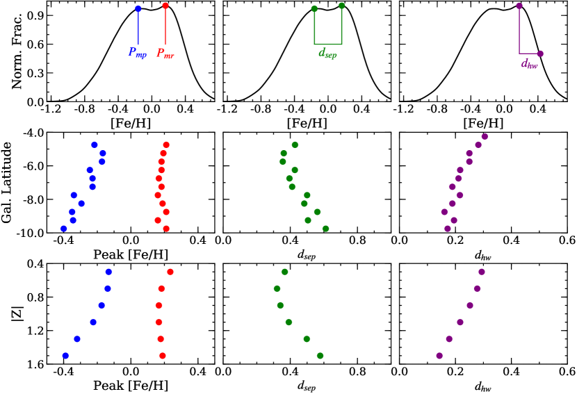
Figure 15: Top: An example metallicity distribution function is shown to highlight the various components that are measured for the lower panels. The top left panel shows how the metal-poor ($P_{mp}$) and metal-rich ($P_{mr}$) peak locations are defined, the middle panel illustrates the distance between peaks ($d_{sep}$), and the right panel indicates the distance between the metal-rich peak and the [Fe/H] value at half power ($d_{hw}$). Middle: the various metrics are measured using the distributions shown in Figure 11. Note that the metal-rich peak remains roughly constant while the metal-poor peak becomes progressively more metal-poor with increasing distance from the plane. Similarly, the $d_{sep}$ parameter also becomes larger with vertical distance. The right panel shows that the metal-rich tail becomes more narrow farther from the plane. Bottom: Identical to the middle panels except measured using Figure 12.

The left panels of Figure 14 compare two sets of chemical enrichment models generated with the One-zone Model for the Evolution of GAlaxies (OMEGA; Côté et al., 2017) code against the observed BDBS metallicity distribution functions derived from stars residing in horizontal stripes centered near |Z| = 0.5 (“inner bulge") and 1.5 kpc (“outer bulge"). For both models, the inflow gas is assumed to have [Fe/H] = $-$1.3 for the metal-poor (blue) model and [Fe/H] = $-$0.5 for the metal-rich (red) model. The metal-poor and metal-rich components of the inner bulge models roughly mimic those presented in Grieco et al. (2012) that have rapid ($<$ 0.3 Gyr) and prolonged ($\sim$ 3 Gyr) star formation time scales, respectively.

Although a detailed modeling of the bulge enrichment history is beyond the scope of this paper, the simple models shown in Figure 14 highlight the possible information content that may be extracted from the distribution morphology, particularly the tails. Changes to the observed metallicity distribution functions that correlate with distance from the plane can be modeled, at least in part, by changing the model inflow/outflow rates, star formation time scales/efficiencies, and/or mass loading factors ($\eta=\frac{\dot{M}_{outflow}}{\dot{M}_{SFR}}$). For the metal-poor component, a combination of higher mass loading factor, longer star formation time scale, and lower star formation efficiency can reduce the effective yield from [Fe/H] = $-0.2$ to $-0.4$ while simultaneously broadening the metal-poor tail. Similarly, enhanced inflow of metal-poor gas helps to truncate the high metallicity tail of the metal-rich component, though an increase in the star formation rate, or the adjustment of a similar lever, is required to maintain the high effective yield. More detailed modeling can be obtained by better constraining these free parameters using the abundance ratios of elements other than Fe.

Nevertheless, the modifications required to match the inner bulge models to the outer bulge data suggest that Galactic winds and related phenomena may have played a strong, and likely detectable, role in shaping the bulge’s star formation history. Consequently, Figure 14 also highlights that the detailed morphologies of the underlying distributions can have a dramatic impact on the assumed contribution from each population. For example, several authors decompose bulge metallicity distributions using Gaussian mixture models (e.g., Ness et al., 2013a; Zoccali et al., 2017; Rojas-Arriagada et al., 2020), but these models generally have little physical motivation and do not account for a population’s likely star formation history. A contrast is seen for the metal-rich component’s shape when comparing Figure 14 to Figure 7 of Zoccali et al. (2017). The former model contributes stars from the metal-rich component down to [Fe/H] $<$ $-0.5$ while the latter fit contributes no stars below [Fe/H] $\sim$ $-0.2$. Additionally, [$\alpha$/Fe] versus [Fe/H] plots of bulge stars (e.g., Figure 1 of Griffith et al., 2021) show that the $\alpha$-enhanced stars span at least [Fe/H] = $-1.5$ to $+$0.3 while the low-$\alpha$ stars span at least [Fe/H] = $-0.5$ to $+$0.5, which is more in agreement with the models shown in Figure 14 and Grieco et al. (2012).

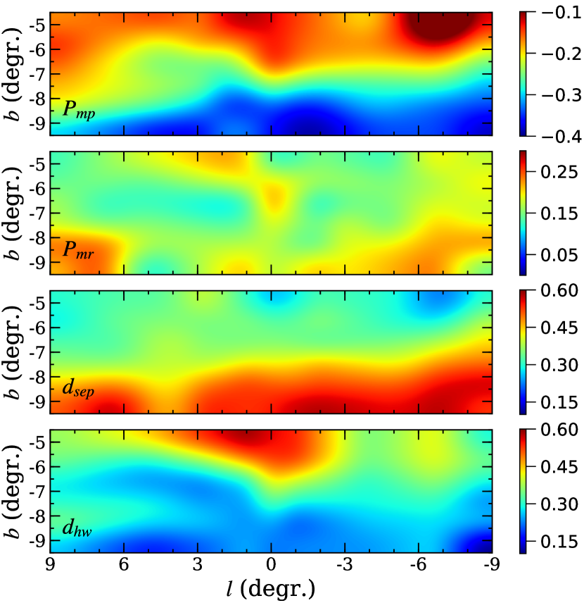
Figure 16: From top to bottom the panels show interpolated maps illustrating the 2D dependence of the metal-poor peak position ($P_{mp}$), metal-rich peak position ($P_{mr}$), separation between the two peaks ($d_{sep}$), and the distance between the metal-rich peak and half-power position of the metal-rich tail ($d_{hw}$), respectively. The color bars are indicative of the [Fe/H] values for each panel (see Figure 15 for definitions of each metric). Note the latitude dependence of the $P_{mp}$ and $d_{sep}$ metrics. The $d_{hw}$ metric generally decreases with increasing distance from the plane (i.e., the metal-rich tail becomes shorter), but some longitudinal dependence is observed for $b>-6^{\circ}$. The metric values were determined in grid points anchored at $l$ = $-$9^∘, $-$7^∘, $-$5^∘, $-$3^∘, $-$1^∘, $+$0^∘, $+$1^∘, $+$3^∘, $+$5^∘, $+$7^∘, and $+$9^∘ along with $b$ = $-4.5$^∘, $-5.5$^∘, $-6.5$^∘, $-7.5$^∘, $-8.5$^∘, and $-9.5^{\circ}$.

Similar to the computed models, Figure 14 shows that the empirical thin and thick disk data from Bensby et al. (2014) are also asymmetric and possess long tails. These combined distribution functions match many of the observed features in the BDBS data, including the general shapes of the metal-poor and metal-rich tails, which follows previous claims noting possible chemical connections between the local disk and bulge (e.g., Meléndez et al., 2008; Alves-Brito et al., 2010; Gonzalez et al., 2011; Jönsson et al., 2017; Zasowski et al., 2019). However, the empirical thin and thick disk distributions must be shifted by $+$0.10 to $+$0.25 dex in [Fe/H] in order to align with the local maxima observed in the bulge distributions. A possible justification for these arbitrary shifts is that the bulge enriched more quickly than the local disk (e.g., Zoccali et al., 2006; Fulbright et al., 2007; Johnson et al., 2011; Bensby et al., 2013, 2017; Rojas-Arriagada et al., 2017; Duong et al., 2019b; Lucertini et al., 2021), and as a result formed from gas that was polluted by material with a higher effective yield. Although the data presented here do not necessarily indicate that the bulge is an inner extension of the disk, Figure 14 shows that the bulge may be well-described by a weighted convolution of two enrichment models that possess properties similar to the thin and thick disks.

4.1.3 Peak Locations

As noted in Section 4.1.1, every field except perhaps those closest to the plane contain two peaks separated by several tenths of a dex in [Fe/H]. Figure 15 illustrates our measurement method and results for tracking the peak [Fe/H] values for the two maxima based on an examination of Figures 11 and 12. The middle left panel of Figure 15 shows that despite a large variation in amplitude across our fields, the metal-rich centroid position remains roughly constant at [Fe/H] $\sim$ $+$0.2. The second panel of Figure 16 further emphasizes the general insensitivity of the metal-rich peak position with bulge location as no strong radial (longitudinal) nor vertical gradients are found. However, Figure 16 does indicate a small number of regions where the metal-rich peak position may be higher than expected, such as along the minor axis with $b$ > $-6^{\circ}$ and near ($l,b$) $\sim$ ($-6^{\circ},-8.5^{\circ}$).

In contrast, the metal-poor centroid position is a strong function of Galactic latitude. Figures 15-16 show that the metal-poor centroid changes from [Fe/H] $\sim-0.15$ at $b\sim-5^{\circ}$ to [Fe/H] $\sim-0.4$ at $b=-9^{\circ}$, in agreement with previous work by Rojas-Arriagada et al. (2014) but contrasting with the seemingly constant metal-poor peak position found by Zoccali et al. (2017, see their Figure 6). Although the metal-poor peak is not as prominent for fields inside |Z| $\sim$ 0.8 kpc in Figure 12, we find an almost identical behavior when examining centroid locations as a function of physical distance from the plane.

Figure 16 does not show a significant longitudinal dependence for $P_{mp}$ in fields with $b>-7^{\circ}$. However, the higher latitude fields show a mild longitudinal correlation such that in sight lines of constant latitude those with positive longitudes have their $P_{mp}$ shifted to higher metallicities than those with negative longitudes. Since the positive longitude fields are dominated by stars on the near side of the bar, it seems likely that the longitudinal gradient in the outer bulge is primarily due to our viewing angle of the bulge/bar system.

Combining the metal-poor and metal-rich trends in the middle panels of Figure 15 illustrates that the separation between the metal-poor and metal-rich peaks becomes larger when moving away from the plane. The third panel of Figure 16 also shows a clearly defined vertical dependence of the $d_{sep}$ metric on latitude along with the same longitudinal dependence as found for the $P_{mp}$ metric. Figure 16 therefore indicates that the vertical gradient in $d_{sep}$ is driven almost entirely by the shifting position of the metal-poor peak that correlates with distance from the plane. This observation suggests that an intrinsic metallicity gradient exists in the bulge, and that the mean metallicity gradient is not driven solely by the mixing of “static" metal-poor and metal-rich populations in different proportions with latitude.

The observed correlation between Z and $P_{mp}$ may be evidence of large-scale events, such as Galactic outflows/winds or inside-out formation, which can shift the metallicity distribution function peak to lower [Fe/H] values at larger distances from the plane (e.g., Boeche et al., 2014; Schlesinger et al., 2014; Schönrich & McMillan, 2017; Nandakumar et al., 2020). Although compelling evidence suggests that disrupted globular clusters have played some role in building up the inner Galaxy stellar populations (e.g., Ferraro et al., 2009; Origlia et al., 2011; Schiavon et al., 2017; Lee et al., 2019; Ferraro et al., 2021), it is unlikely that such a mechanism would produce the observed metal-poor gradient.

4.1.4 Mean Metallicity Gradient

The mean metallicities provided in the panels of Figures 11 and 12 indicate that a strong vertical metallicity gradient is present in the bulge. In particular, the mean [Fe/H] value decreases from $\sim$ $+$0.1 near the plane to $-0.3$ in fields $>$ 1.5 kpc from the plane. However, we find no significant differences in mean [Fe/H] values for the three most interior fields of Figure 11, which suggests that the metallicity gradient may be significantly flatter for $|b|<-5^{\circ}$. Additionally, we find that the dominant composition gradient is in the vertical, rather than radial, direction (see also Section 4.3).

Using the values presented in Figure 11, we measure a metallicity gradient between $b=-3.5^{\circ}$ and $-10^{\circ}$ of d[Fe/H]/d$b$ = $-0.05$ dex degree^-1. This is equivalent to a metallicity gradient of d[Fe/H]/dZ = $-0.38$ dex kpc^-1 in physical coordinates for fields with 0.5 < |Z| < 1.5 kpc. Our measured mean metallicity gradient values are almost identical to those obtained when fitting a linear function to the changing peak [Fe/H] values of the metal-poor population shown in Figure 15. Specifically, we find the gradient in the metal-poor peak centroid location to be d[Fe/H]/d$b$ = $-0.04$ dex degree^-1, which is equivalent to d[Fe/H]/dZ = $-0.37$ dex kpc^-1 in physical dimensions.

4.1.5 Metal-rich Tail Variations

A more subtle change in the metallicity distribution function morphology can be seen upon close inspection of the metal-rich tails in Figures 11 and 12. Although the metal-rich peak centroids remain stable across all slices, the distribution shape at higher metallicities appears to become truncated when examining higher latitude fields.

We investigated the potential metal-rich tail variations using the right panels of Figure 15, which measure the distance between the metal-rich peak centroid and the [Fe/H] value corresponding to half the peak amplitude ($d_{hw}$). Figure 15 indicates that the metal-rich tail forms a progressively narrower distribution at larger distances from the plane. In fact, the $d_{hw}$ parameter exhibits a gradient of d($d_{hw}$)/d$b$ = $-$0.02 dex degree^-1, which is equivalent to d($d_{hw}$)/d$Z$ = $-$0.16 dex kpc^-1. It is possible that differences in star formation efficiency, infall times, and/or outflow may be driving the varying metal-rich tail widths as functions of vertical distance (e.g., Mould, 1984; Ballero et al., 2007). Similarly, sudden gas removal that becomes more efficient farther from the plane could drive a sharper metal-rich cut-off at higher latitudes, as is observed in dwarf spheroidal galaxies (e.g., Koch et al., 2007; Kirby et al., 2011).

Figure 16 confirms that $d_{hw}$ generally decreases with increasing distance from the plane, although some mild longitudinal dependence may also be present for fields outside $b=-6^{\circ}$. A much stronger longitudinal dependence is found for fields with $b>-6^{\circ}$. Sight lines near the minor axis ($|l|<3^{\circ}$) have noticeably longer metal-rich tails than fields with $|l|>3^{\circ}$, perhaps as a consequence of inside-out formation of the early bulge. This observation is further supported by evidence presented in Sit & Ness (2020) that for fields close to the plane the metallicity dispersion reaches a maximum near the Galactic Center but decreases when moving outward along the major axis. We note also that the region of maximum $d_{hw}$ in Figure 16 also coincides with a population of stars having noticeably higher $\sigma_{\mu_{b}}$ compared to those in adjacent fields (see Figure 10 of Clarke et al., 2019).

We caution that the $d_{hw}$ metric could be particularly sensitive to RGB contamination in the red clump region. The contamination simulations presented in Figure 9 do produce broader metal-rich tails when RGB contamination is accounted for. Alternatively, the length of the metal-rich tail could be sensitive to reddening uncertainties, with weaker tails appearing at higher latitudes due to intrinsically reduced differential extinction (see also the bottom panel of Figure 7). However, as noted previously the [Fe/H] dispersion for the metallicity distribution in a given field is only weakly dependent on latitude.

4.1.6 Literature Comparisons

Figure 17 compares the BDBS derived metallicity distribution functions against those in similar fields from the ARGOS, Gaia-ESO, APOGEE, A2A, GIBS, and HERBS spectroscopic surveys. Despite the variety in sample sizes, data quality, and analysis methods, we can note several common patterns that are reproduced by all surveys: (1) clear morphological changes in the metallicity distributions that are correlated with vertical distances from the Galactic plane; (2) most fields appear to have at least two local maxima; (3) all fields exhibit large metallicity ranges spanning at least $-1<$ [Fe/H] $<+0.5$; and (4) the mean metallicity decreases with increasing distance from the plane (i.e., a vertical metallicity gradient exists).

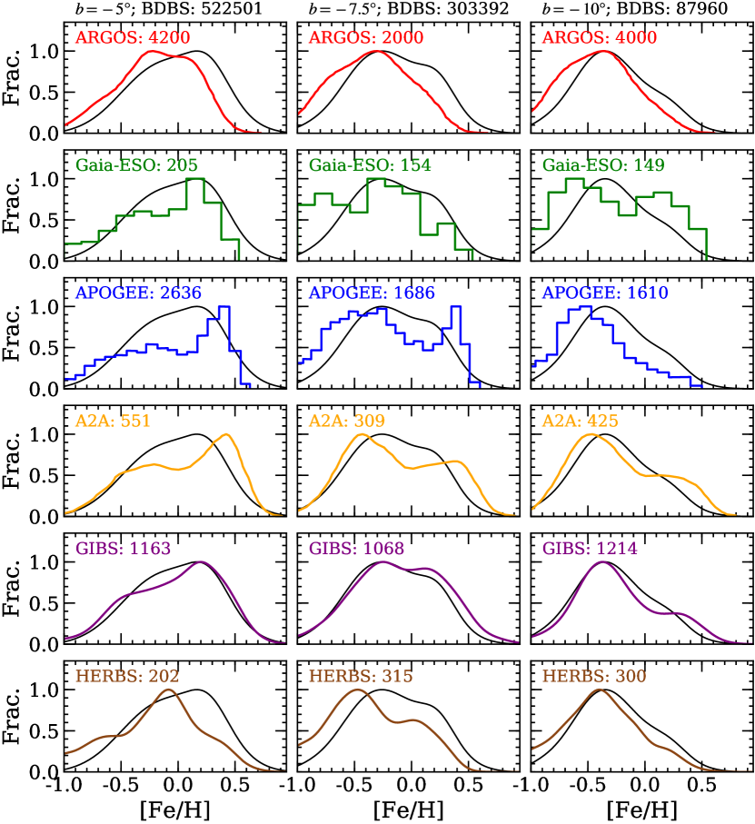
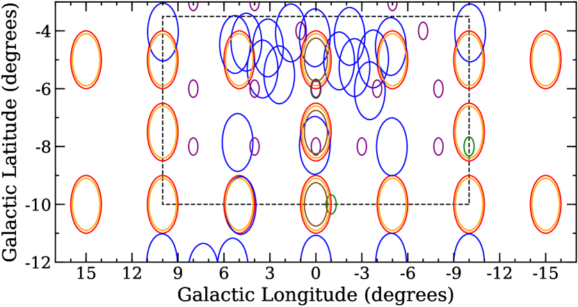
Figure 17: Top panels: BDBS metallicity distribution functions (black lines) are compared against similar data from the ARGOS (red; Ness et al., 2013a), Gaia-ESO (green; Rojas-Arriagada et al., 2014), APOGEE (blue; Rojas-Arriagada et al., 2020), A2A (orange; Wylie et al., 2021), GIBS (purple; Zoccali et al., 2017), and HERBS (brown; Duong et al., 2019a) surveys. Histogram values for all data sets except GIBS and HERBS, which provided data tables, were measured off the published figures. The number of stars in each distribution is provided with each panel. The data cover all longitudes in each sample when available, and generally span about $\pm$ 1^∘ in latitude around $b=-5^{\circ}$ (left), $b=-7.5^{\circ}$ (middle), and $b=-10^{\circ}$ (right). Bottom panel: Approximate field centers and sizes are outlined for each survey. The colors of the fields match the histograms in the top panels, and the dashed box highlights the approximate coverage of the BDBS data presented here. For overlapping sight lines, the field sizes have been slightly modified for visibility.

Further examination of Figure 17 reveals several important differences between the surveys. For example, both the number of local maxima and their associated peak [Fe/H] locations are not consistent; however, at least some of this discrepancy is driven by differences in analysis methods, data quality, and wavelengths. These morphological differences are particularly troublesome when comparing the ARGOS, A2A, and HERBS distributions, which have significant sample overlap. Interestingly, the metallicity distributions appear to converge when observing fields farther from the plane.

For the inner bulge fields near $b=-5^{\circ}$, the metal-poor tails of all seven surveys shown in Figure 17 are surprisingly similar, at least for $-1<$ [Fe/H] $<-0.4$. Most of the surveys also show the same pattern of a dominant metal-rich peak near [Fe/H] $\sim$ $+$0.2. However, the ARGOS and HERBS data sets have a paucity of very metal-rich stars. The Gaia-ESO data exhibit a truncated metal-rich tail compared to BDBS, APOGEE, and GIBS while the A2A metal-rich peak appears shifted to a relatively high value ([Fe/H] $>$ $+$0.4). We can also note that the global maximum for the HERBS distribution occurs near the same metallicity ([Fe/H] $\sim$ $-$0.2) at which the Gaia-ESO, APOGEE, and A2A data exhibit clear local minima.

At $b=-7.5^{\circ}$, the BDBS distribution is morphologically similar to those of the GIBS and A2A surveys. Figure 17 also indicates that the BDBS and HERBS distributions may be very similar when taking into account a possible $\sim$0.2 dex zero-point offset. However, the ARGOS and Gaia-ESO data show significantly more stars with [Fe/H] $<$ $-0.8$. Although sample selection may explain part of this discrepancy, we note that most of the surveys shown in Figure 17 targeted red clump stars. Similar to the $b=-5^{\circ}$ distributions, we note that the ARGOS sample has a much smaller number of very metal-rich stars compared to most other surveys. The metal-rich peak locations are also at least 0.1-0.2 dex higher for the Gaia-ESO, APOGEE, and A2A distributions compared to those of BDBS, GIBS, and HERBS.

Unlike the fields closer to the plane, the $b=-10^{\circ}$ distributions are all morphologically similar with strong metal-poor peaks near [Fe/H] $\sim$ $-0.4$ and long metal-rich tails. The ARGOS, GIBS, A2A, and HERBS data sets seem to require zero-point offsets of $\sim$0.1 dex or less to align with BDBS while those of Gaia-ESO and APOGEE are offset by $\sim$0.1-0.3 dex. Although the ARGOS metal-rich tail is now more similar to those of other surveys, the prominent very metal-poor peak at [Fe/H] $\sim$ $-0.8$ is not generally observed in other data sets. The Gaia-ESO distribution shows noticeably more stars with [Fe/H] $>$ 0 than any other survey, despite having a metal-rich peak at about the same location.

Finally, we can compare the mean metallicity gradient derived here against those in the literature. As noted in Section 4.1.4, we find d[Fe/H]/d$b$ = $-0.05$ dex degree^-1 or d[Fe/H]/dZ = $-0.38$ dex kpc^-1 for fields with $-10^{\circ}<b<-3.5$ and 0.5 < |Z| < 1.5 kpc, respectively. These values are in excellent agreement with previous estimates ranging from d[Fe/H]/d$b$ = $-0.04$ to $-0.075$ dex degree^-1 in observed coordinates (Zoccali et al., 2008; Gonzalez et al., 2013; Rojas-Arriagada et al., 2014) and spanning d[Fe/H]/dZ = $-0.6$ to $-0.24$ dex kpc^-1 in physical coordinates (Zoccali et al., 2008; Johnson et al., 2013; Ness et al., 2013a; Rojas-Arriagada et al., 2017, 2020; Wylie et al., 2021). Figure 15 indicates that the metallicity gradient might become more shallow for |Z| $<$ 0.5 kpc, which would be in agreement with previous analyses (Rich et al., 2007b, 2012; Schultheis et al., 2019; Rojas-Arriagada et al., 2020); however, our observations do not extend close enough to the plane to confirm this trend.

4.2 The X-Shape in BDBS Data

Using the observed Galactic coordinates in concert with the adopted relationships between [Fe/H], $M_{i,o}$, and distance outlined in Equations 6-7, we can construct three dimensional density maps of the red clump distributions as functions of metallicity. Figure 18 shows three vertical slices through the density maps out to |Z| = 1.3 kpc and for three broad metallicity bins. The figure also includes contour projections from Simion et al. (2017) that fit the VVV density distribution of the bulge/bar inside |Z| = 0.7 kpc and a separate parameterization of the X-shape structure from López-Corredoira (2017) in the outer bulge fields.

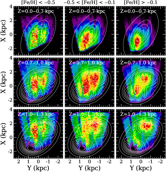
Figure 18: The top, middle, and bottom rows show density map slices (as if viewing the bulge from the North Galactic Pole) of BDBS red clump stars in physical coordinate space with |Z| values ranging from 0.0-0.7 kpc, 0.7-1.0 kpc, and 1.0-1.3 kpc, respectively. Similarly, the left, middle, and right columns only include stars with [Fe/H] $<$ $-0.5$, $-0.5<$ [Fe/H] $<-0.1$, and [Fe/H] $>$ $-0.1$, respectively. In all panels, the highest density regions have red and orange colors while the lowest density regions have black and purple colors. For the top row, the contours show a slice of the best fit 3D density law that best describes the VVV density distribution (Simion et al., 2017, their model E, equation 2; see also their Table 3) projected along the Z-axis between 0.0 and 0.7 kpc. The contours for the middle and bottom rows show the projection of the X-shape density function provided by López-Corredoira (2017), which is a parameterization of the double red clump at intermediate latitudes based off of previous models by López-Corredoira et al. (2005) and Wegg & Gerhard (2013).

Visual inspection of Figure 18 shows that close to the plane (|Z| $<$ 0.7 kpc) our observations are skewed to favor metal-rich ([Fe/H] $>$ $-0.5$) stars on the near side of the bar. Although some previous studies found evidence of the X-shape structure emerging as low as $\sim$ 400 pc from the plane (e.g., Wegg & Gerhard, 2013), we did not find any X-shape signatures for distances inside $\sim$ 700 pc. The most metal-poor stars in our sample ([Fe/H] $<$ $-0.5$) appear to be more uniformly distributed than the more metal-rich stars, and exhibit a peak near the Galactic center (X = 0 kpc). This observation provides evidence that metal-poor stars in the bulge are distributed differently than those with [Fe/H] $>$ $-0.5$, as has been previously noted by several authors (e.g., Ness et al., 2013a; Rojas-Arriagada et al., 2014; Zoccali et al., 2017; Rojas-Arriagada et al., 2020). However, we note that Kunder et al. (2020) found evidence supporting two RR Lyrae populations co-existing in the bulge: one is constrained to within the inner 3.5 kpc of the Galactic Center and follows the bar while the other is more centrally concentrated but does not trace the bar. We suspect that a subset of our metal-poor sample traces the same population as the barred RR Lyrae, and that the fractional weights of the barred versus non-barred groups vary with vertical distance from the plane. Nevertheless, our observations reinforce previous velocity ellipsoid analyses that found a significant vertex deviation consistent with bar-like kinematics only exists for stars with [Fe/H] $>$ $-0.5$ (Soto et al., 2007; Babusiaux, 2016; Simion et al., 2021).

At intermediate distances from the plane (0.7 $<$ |Z| $<$ 1.0 kpc), Figure 18 shows that the most metal-poor stars have little connection with the shape of the bar, and instead exhibit a more isotropic distribution centered near X = 0 kpc. In contrast, the spatial distributions for the intermediate and high metallicity bins strongly align with the modeled bar angle (20^∘). Stars with [Fe/H] $>$ $-0.5$ appear to cluster in two high density regions on the near and far sides of the bar around X $\sim$ $\pm$ 1 kpc, similar to what Li & Shen (2012) found with their N-body Milky Way bulge model. In fact, the local maxima of these regions are very similar in position and extent to the X-shape contours that are evaluated between |Z| = 0.7-1.0 kpc. The middle panel of Figure 18 provides evidence that the high density regions for stars with $-0.5<$ [Fe/H] $<-0.1$ may be more extended along the Sun-Galactic Center (X) coordinate than higher metallicity stars. However, this could also be a result of mixing stars that are more isotropically distributed with those of somewhat higher metallicity that are concentrated within the X-shape structure. Alternatively, the larger extension in the X coordinate for intermediate metallicity stars could be a result of a thicker X-shape structure and/or “contamination" from the far end of the X-shape. We note also that Li & Shen (2015) showed that the X-shape is likely to have a broader, peanut-shaped morphology than a well-defined and thin shape like the letter X.

For the largest vertical distance slice shown in Figure 18, the metal-poor stars still appear more isotropically distributed, but the highest density regions are found 0.5-1.0 kpc beyond the Galactic Center. The shift in the peak position of metal-poor stars to larger distances is likely a result of the viewing angle along lines of sight that intersect |Z| = 1.0-1.3 kpc, rather than an intrinsic change in the distribution. Similar to the |Z| = 0.7-1.0 kpc vertical slices, the intermediate and metal-rich bins again show clear over-densities that are well-aligned with both the bar angle and the X-shape model. However, since the BDBS map does not currently include measurements of stars with $b\la-9^{\circ}$ for fields with $l\ga+3^{\circ}$ (e.g., see Figure 1 of Johnson et al., 2020), we are only able to partially detect the X-shape structure on the near side of the bar (see also Gonzalez et al., 2015). The over-density on the far side of the bar almost exactly matches the model contours in location, extent, and shape. Furthermore, the separation between the near and far side metal-rich over-densities becomes larger with increasing vertical distance, which suggests that we are directly observing the X-shape structure in the bulge.

4.3 Metallicity Dependent Spatial Distributions

Previous surveys have established that the observed metallicity gradient is likely driven by changes in the vertical scale height of bulge stars with different mean metallicities (e.g., Zoccali et al., 2008; Hill et al., 2011; Ness et al., 2013a; Zoccali et al., 2017; Duong et al., 2019a; Rojas-Arriagada et al., 2020). In Figure 19, we show the spatial distribution of red clump stars in the BDBS survey area with different metallicities, and confirm that the vertical scale heights change strongly as a function of metallicity.

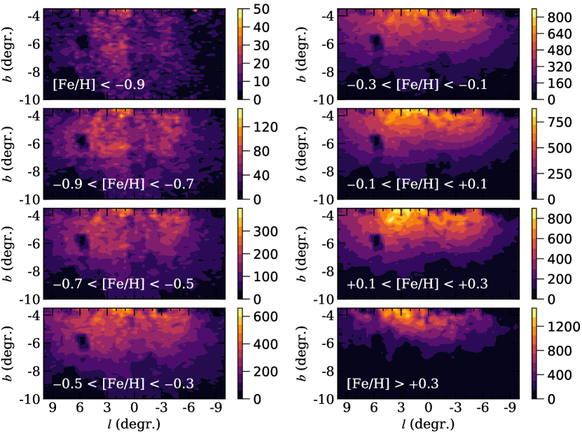
Figure 19: Red clump density distribution contours are shown in observed coordinates for several metallicity bins. The total number of stars in each panel ranges from $\sim$ 20,000 in the most metal-poor bin to $>$ 500,000 in the most metal-rich bin. A clear change in the spatial distribution is observed for stars on either side of [Fe/H] $\sim$ $-0.3$. The metal-poor stars extend to high latitudes and appear to exhibit a more spheroidal distribution. In contrast, the metal-rich stars are concentrated close to the plane and exhibit a boxy/peanut morphology.

Further visual inspection of Figure 19 reveals strong morphological changes in the spatial distributions as a function of metallicity as well. For example, stars with [Fe/H] $<$ $-0.3$ almost uniformly fill the BDBS footprint area and lack any clear structure. However, we systematically observe about 5 per cent more stars with [Fe/H] $<$ $-0.3$ at positive longitudes than negative longitudes, which suggests that the metal-poor stars may form an oblate spheroid that is at least weakly aligned with the bar. Starting with the $-0.3<$ [Fe/H] $<-0.1$ bin in Figure 19, the outer contours become more rounded and/or peanut-shaped while simultaneously exhibiting a retreat to smaller Galactic latitude values. The peanut shape is less obvious in the highest metallicity bin, but this is likely due to the strong concentration near the plane for these stars coupled with our limited observations inside $b=-4^{\circ}$. Additionally, these stars may form a more “central boxy core" that is less peanut-shaped, as discussed in Li & Shen (2015). The metallicity dependent spatial variations observed here are consistent with previous investigations of Mira stars that found the older, more metal-poor stars traced a spheroid while the younger, more metal-rich population exhibited a barred structure (Catchpole et al., 2016; Grady et al., 2020).

Changes to the vertical distributions of bulge stars are further illustrated in Figure 20, which plots the red clump star counts and fractional compositions as functions of vertical distance from the plane. We find that the number densities of stars with [Fe/H] $<$ $-0.3$ only change by about a factor of 2-10 between the most inner and outer fields sampled in Figure 20. This observation is consistent with previous assertions that most of the metal-poor stars in the bulge likely form either an oblate spheroid or “thick bar" distribution, which is also supported by kinematic arguments (e.g., Babusiaux et al., 2010). A combination of the observed spatial distribution and shifting metal-poor peak position with latitude may be useful for constraining dissipative collapse or gas outflow parameters in future models.

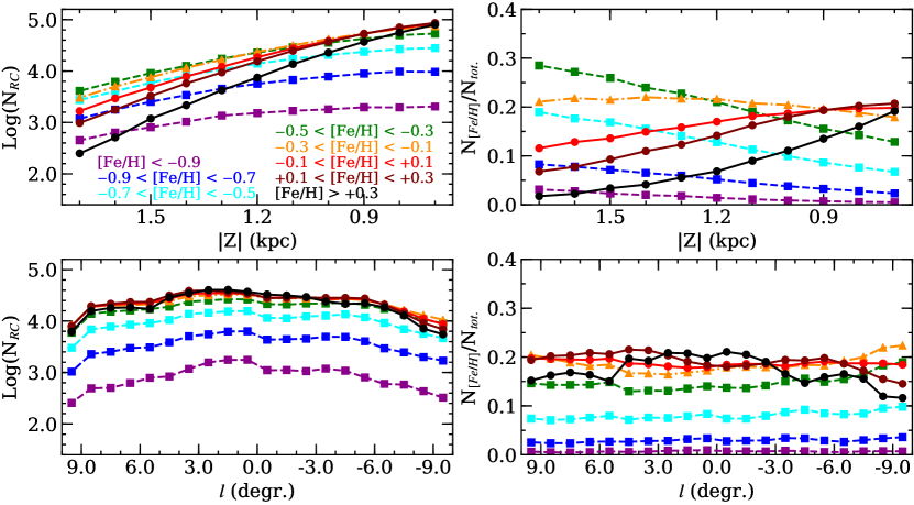
Figure 20: The top left panel plots the log of the number of red clump stars in 0.1 kpc vertical stripes, summed across all longitudes, for the metallicity bins shown in Figure 19. The bottom left panel plots the ratio of the number of red clump stars within a given metallicity bin against the total number of red clump stars in each vertical stripe. This panel highlights two broad “families" that show different dependencies with distance from the plane, which are also correlated with [Fe/H]. Groups with decreasing fractions at lower latitudes are indicated with filled boxes and dashed lines, those with a flat functional form are indicated with filled triangles and dot-dashed lines, and those with increasing functions have filled circles and solid lines. The bottom panels show similar plots as a function of Galactic longitude, summed across all latitudes, and highlight that no similar metallicity-dependent gradient is found in the radial direction.

In contrast to the metal-poor vertical distributions, Figure 20 shows that more metal-rich stars exhibit substantial increases in red clump number densities when moving from the outer to inner bulge, and that the rate of increase is strongly correlated with chemical composition. For example, the number of red clump stars with $-0.1<$ [Fe/H] $<+0.1$ increases by about a factor of 60 between |Z| = 1.7 and 0.7 kpc. However, over the same distance the number of red clump stars with [Fe/H] $>$ $+0.3$ increases by a factor of 400.

The strong correlation between vertical slice star counts and metallicity is also reflected in the right panels of Figure 15, which show that the metal-rich tails becomes broader closer to the plane. Such observations may reflect variations in either the star formation efficiency or gas infall times in the bulge, which are likely to increase the width of the resulting metallicity distribution functions without shifting the metal-rich peak position (e.g., Ballero et al., 2007).

The top right panel of Figure 20, which shows the change in the ratios of stars within a given metallicity bin to the total number of stars in a vertical slice, also support the presence of two broad stellar groups. The metallicity bins that include stars with [Fe/H] $<$ $-0.3$ all exhibit the same basic pattern where their fractional contributions have maximums in the outer bulge and then monotonically decrease when moving closer to the plane. Similarly, all of the metallicity bins that include stars with [Fe/H] $>-0.1$ increase their $N_{[Fe/H]}/N_{tot.}$ ratios monotonically from the outer to inner bulge.

The $-0.3<$ [Fe/H] $<-0.1$ metallicity bin maintains a nearly constant $N_{[Fe/H]}/N_{tot.}$ ratio of about 0.2, and signals a transition between the two groups. This metallicity bin aligns roughly with the [$\alpha$/Fe] inflection point found near [Fe/H] $\sim$ $-0.3$ (e.g., Fulbright et al., 2007; Alves-Brito et al., 2010; Gonzalez et al., 2011; Johnson et al., 2011; Bensby et al., 2017; Rojas-Arriagada et al., 2017; Duong et al., 2019a), and also with the vertex deviation at [Fe/H] $\sim$ $-0.5$ observed in some minor-axis bulge fields (Zhao et al., 1994; Soto et al., 2007; Babusiaux et al., 2010; Soto et al., 2012; Simion et al., 2021). The bottom panels of Figure 20 highlight the lack of any similar metallicity gradient in the radial (longitudinal) direction.

A comparison of the metal-poor and metal-rich red clump distributions shown in Figure 20 with the Gaussian decompositions presented in Zoccali et al. (2017) leads to an apparent conflict of results. Extrapolating the star counts of each metallicity bin in Figure 20 from the last reference point toward the plane should result in a continued increase in the prominence of stars with [Fe/H] $>$ $-0.1$ concurrent with a strong (relative) decrease in the fraction of stars with [Fe/H] $<$ $-0.5$. However, Figure 7 of Zoccali et al. (2017) shows that the metal-poor component decreases in fractional contribution between $b=-8.5^{\circ}$ and $-3.5^{\circ}$, and then increases again at latitudes closer to the plane.

Although the BDBS data cannot rule out an increase in the metal-poor star count trends for fields with $b>-3.5^{\circ}$, a possible explanation, as mentioned in Section 4.1.2, is that the metal-poor and metal-rich groups are not well-represented as Gaussian distributions. Instead, these broad groups are likely skewed distributions with long tails, which can lead to over/under-counting fractional compositions when using Gaussian mixture models. If we assume the |Z| = 0.5 and 2.0 kpc distributions of Figure 13 are close representations of the true metal-poor and metal-rich groups, respectively, then we find that sight lines with strong metal-rich peaks will naturally contain substantial numbers of metal-poor stars. Furthermore, as mentioned in Section 4.1.5, we also find evidence that the metal-rich tail becomes broader closer to the plane, and especially along the minor-axis. A broadening of the metal-rich metallicity distribution function might also strengthen the population’s metal-poor tail such that it mimics a growing contribution from the separate metal-poor group.

Therefore, we posit that the large population of metal-poor stars found in fields close to the plane by Zoccali et al. (2017) may be driven more by the metal-rich group’s metal-poor tail than the rising prominence of a truly separate metal-poor population. In fact, we argue that the bulge may contain two distinct metal-poor populations: one group is the metal-poor tail of the star formation event that produced the metal-rich peak while the other is the vertically extended spheroidal population that dominates at high latitudes. This assertion is consistent with the chemodynamical results presented by Queiroz et al. (2020) that indicate two or more metal-poor populations co-existing in the bulge that possess different kinematic signatures.

We also note Zoccali et al. (2017) found that while metal-poor stars have higher velocity dispersions than metal-rich stars in the outer bulge, the two populations have similar velocity dispersions between $b=-3.5^{\circ}$ and $-2.0^{\circ}$. Zoccali et al. (2017) attributed this result to the metal-poor population hosting a velocity gradient; however, one might also expect a similar observation if a majority of stars within a few degrees of the plane are actually part of the same population that produced the metal-rich peak. If the inner few degrees of the bulge are dominated by a single long-tailed distribution then this would support previous observations showing that the metallicity gradient flattens out and does not extend to the inner bulge (Rich et al., 2007b, 2012; Schultheis et al., 2019; Rojas-Arriagada et al., 2020).

5 Summary

For this work, we have isolated a sample of $\sim$ 2.6 million red clump stars spanning $|l|<10^{\circ}$ and $-10^{\circ}<b<-3.5^{\circ}$ from the BDBS catalog (Johnson et al., 2020; Rich et al., 2020). We applied Gaia EDR3 proper motions and parallaxes to remove likely foreground contamination, and also determined distance estimates from a metallicity-dependent calibration of dereddened $i$-band photometry based on 10 Gyr stellar isochrones. Metallicities were determined for each red clump star using the calibration between BDBS $(u-i)_{o}$ colors and spectroscopic GIBS [Fe/H] values presented in Johnson et al. (2020). Using these data, we derived metallicity distribution functions and three dimensional density maps over most of the BDBS footprint. A summary of the results includes:

• In agreement with past work, we find a strong change in the metallicity distribution function morphology that varies with vertical distance from the plane. However, the metallicity distribution functions generally have a weak dependence on longitude.

• Metallicity distributions for fields close to the plane ($b\sim-4^{\circ}$) are asymmetric, strongly peaked near [Fe/H] $\sim$ $+$0.2, and possess a long metal-poor tail. A clear second and more metal-poor peak emerges starting at $b\sim-5^{\circ}$ and grows in prominence with increasing distance from the plane. Additionally, while the metal-rich peak remains fixed near [Fe/H] = $+$0.2 for all latitudes, the metal-poor peak shifts from [Fe/H] $\sim$ $-0.15$ to $-0.4$ between $b\sim-4^{\circ}$ and $-10^{\circ}$ (0.5 $<$ |Z| 1.5 kpc), respectively. A third, more metal-poor peak near [Fe/H] $\sim$ $-0.8$ is found along a few sight lines but only for |Z| $\sim$ 2 kpc.

• Overall, the mean metallicity decreases from [Fe/H] = 0 at $b=-3.75^{\circ}$ to [Fe/H] = $-0.3$ at $b=-9.75^{\circ}$. Similar results are found if the data are binned by physical distance from the plane (Z) rather than observed Galactic latitude. The main difference when binning by Z is that these metallicity distribution functions appear to have somewhat sharper peaks and tails, likely due to the removal of stars at different Z distances that “contaminate" the distribution when integrating along a line of constant Galactic latitude.

• Using the inner and outermost fields as representations of the true underlying metal-poor and metal-rich populations, we find that the metallicity distribution function morphologies are likely not well-represented by Gaussian functions. Instead, the two components may be more similar to the asymmetric, long-tailed morphologies generated either by chemical enrichment models or from empirical local thin and thick disk metallicity distribution functions. However, the bulge populations are generally at least 0.2 dex more metal-rich than the local thin and thick disk stars.

• Similar to previous studies, we find a clear vertical metallicity gradient equivalent to $-0.05$ dex degree^-1 ($-0.38$ dex kpc^-1) for sight lines between $b=-3.5^{\circ}$ and $-10^{\circ}$ (|Z| = 0.5 to 1.5 kpc). Additionally, we find a clear negative gradient for the metal-poor peak position of $-0.04$ dex degree^-1 ($-0.37$ dex kpc^-1), which is nearly identical to the mean metallicity gradient. The observed correlation between the metal-poor peak position and distance from the plane could have been driven by galaxy-scale mechanisms, such as winds/outflows or inside-out star formation, rather than accretion or the tidal destruction of globular clusters.

• An interesting new result presented here is the correlation between the metal-rich tail width and distance from the plane. We find that the metal-rich tails truncate more sharply after the peak in higher latitude fields compared to those closer to the plane. Additionally, we find in fields with $b>-6^{\circ}$ that sight lines along the minor axis ($|l|<3^{\circ}$) have longer metal-rich tails than those farther from the Galactic Center.

• Extracting slices of constant Z through the BDBS data set revealed clear evidence of metallicity dependent variations in the spatial density distributions. In agreement with past work, stars with [Fe/H] $<$ $-0.5$ show only a weak connection to the bar and appear more isotropically distributed than their more metal-rich counterparts. The stars with [Fe/H] $<$ $-0.5$ also do not show any evidence of participating in orbits that support the X-shape structure. In contrast, stars with [Fe/H] $>$ $-0.5$ follow the bar orientation at all vertical distances.

• For fields with |Z| $>$ 0.7 kpc, stars with [Fe/H] $>$ $-0.5$ exhibit two spatially concentrated, high density regions on either side of the Galactic Center that align with the bar angle. Furthermore, the separation between the two over-densities increases with distance from the plane, and a comparison between the observed distributions and a parametric model reveals that these over-densities match the predicted contours of the X-shape structure.

• Metallicity dependent red clump density contour maps reveal a strong change in the 2D spatial distribution of stars as a function of metallicity as well. Stars with [Fe/H] $<$ $-0.3$ span the entire BDBS footprint and appear to form an oblate spheroid or thick bar distribution. In contrast, starting at [Fe/H] $\sim$ $-0.3$ stars begin to form a clear boxy/peanut shape structure that is associated with the inner disk/bar. However, the peanut shape is less defined for stars with [Fe/H] $>$ $+$0.3 that are close to the plane, which may suggest that the inner portion of the bulge forms more of a central boxy core, as noted in Li & Shen (2015). We also find that the vertical extent of stars rapidly decreases with increasing metallicity, especially for [Fe/H] $>$ 0.

• In general, we find evidence of two broad distributions where stars with [Fe/H] $<$ $-0.3$ exhibit declining fractional contributions when moving closer to the plane while those with [Fe/H] $>$ $-0.1$ exhibit increasing fractional contributions. Stars with $-0.3<$ [Fe/H] $<-0.1$ serve as a transition point and exhibit a nearly constant N${}_{[Fe/H]}/N_{tot.}$ ratio of about 0.2 across all latitudes investigated here.

• The vertical number density distributions are also sensitive functions of [Fe/H]. For example, the number of stars with [Fe/H] $<$ $-0.3$ only increases by about a factor of 2-10 between $b=-10^{\circ}$ and $-4^{\circ}$. However, stars with $-0.1<$ [Fe/H] $<+0.1$ increase by a factor 60 and stars with [Fe/H] $>$ $+$0.3 increase by a factor of 400 over that same vertical range.

• The monotonically decreasing fractional contributions of metal-poor stars with decreasing distance from the plane seems to contrast with the results of Zoccali et al. (2017), which showed that the metal-poor population reaches a minimum near $|b|$ $\sim$ 3.5^∘ and increases when moving closer to the plane. We argue instead that the bulge has two metal-poor populations: one that forms the long metal-poor tail of the distribution that peaks near [Fe/H] = $+$0.2 and the other that belongs to the metal-poor population that dominates in the outer bulge. The existence of two or more metal-poor groups is supported by chemodynamical data presented in Queiroz et al. (2020). We note also that the inner bulge being mostly dominated by a single asymmetric, long-tailed metallicity distribution would help explain observations finding a weak or null metallicity gradient within a few degrees of the plane.

The photometric metallicity maps presented here offer new insight into the bulge’s formation history, and in the future may be combined with future Gaia data releases to obtain accurate chemodynamical maps encompassing millions of red clump stars. These data also offer a glimpse at the type of science that may be achieved with upcoming observations from the Vera C. Rubin Observatory, and highlight the critical role wide-field $u$-band observations can fill for reconstructing the Galaxy’s formation history.

Data Availability

The raw and pipeline reduced DECam images are available for download on the NOAO archive at http://archive1.dm.noao.edu/. Astrometric, photometric, and reddening catalogs are in the process of being prepared for public release. The data used in this paper are provided in an electronic table, but further information, including an extended release of BDBS data beyond what is presented here, may be provided upon request to the corresponding author.

Table 1: Bulge Red Clump Data

RA	DEC	$u$	$u_{err}$	$g$	$g_{err}$	$i$	$i_{err}$	$A_{u}$	$A_{g}$	$A_{i}$	Dist.	$\sigma$ Dist.	[Fe/H]	$\sigma$ [Fe/H]
(degrees)	(degrees)	(mag.)	(mag.)	(mag.)	(mag.)	(mag.)	(mag.)	(mag.)	(mag.)	(mag.)	(kpc)	(kpc)	(dex)	(dex)
263.73815	$-$39.34179	22.866	0.229	19.830	0.007	17.064	0.016	4.682	3.738	2.030	8.731	0.858	$-$0.30	0.49
263.81260	$-$39.36577	22.640	0.037	19.964	0.003	17.220	0.007	5.204	4.154	2.256	8.754	0.886	$-$0.68	0.53
263.83048	$-$39.34130	22.891	0.451	20.358	0.000	17.639	0.006	5.073	4.050	2.200	10.951	1.150	$-$0.73	0.58
263.83091	$-$39.36591	22.933	0.235	20.543	0.012	17.732	0.006	5.236	4.180	2.270	11.146	1.147	$-$0.82	0.55
263.83457	$-$39.34498	23.077	0.246	20.173	0.002	17.342	0.006	5.041	4.024	2.186	9.366	0.949	$-$0.45	0.53
…	…	…	…	…	…	…	…	…	…	…	…	…	…	…
280.70911	$-$24.54837	19.553	0.001	17.440	0.008	16.090	0.003	1.146	0.915	0.497	11.492	0.769	$-$0.49	0.12
280.71047	$-$24.54482	18.874	0.004	16.538	0.002	15.127	0.017	1.146	0.915	0.497	7.269	0.490	$-$0.33	0.12
280.71134	$-$24.54170	19.413	0.001	17.173	0.001	15.821	0.025	1.146	0.915	0.497	10.086	0.686	$-$0.42	0.12
280.71366	$-$24.54457	19.690	0.017	17.066	0.008	15.664	0.001	1.146	0.915	0.497	9.175	0.614	$-$0.17	0.12
280.71960	$-$24.51606	19.308	0.016	17.261	0.017	15.933	0.029	1.187	0.948	0.515	10.665	0.732	$-$0.55	0.12
The full version of this table is provided in electronic form.

Appendix A Luminosity and Color Cuts for Red Clump Stars

We provide additional examples of luminosity and color functions in the red clump regions of 21 fields spanning a large fraction of the BDBS footprint. The dashed red lines in Figure 21 show the selection criteria when adopting the bright and faint magnitude limits presented in Equations 1 and 2. The data show that we sufficiently encapsulate the red clump region, regardless of whether a single or double red clump feature is present. Figure 21 also shows the expected behavior of the red clump becoming fainter at more negative longitudes, which is consistent with the bar viewing angle.

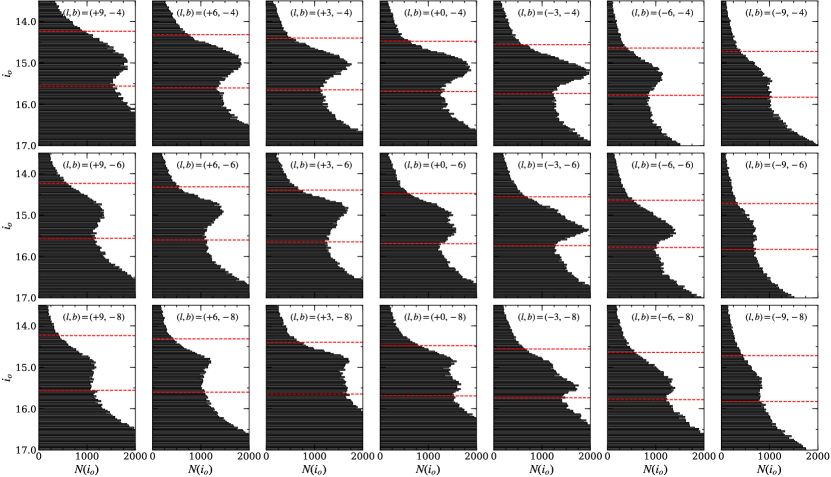
Figure 21: Similar to the middle panels of Figure 2, $i_{o}$ magnitude selection limits (dashed red lines) for bulge red clump stars are shown for a variety of fields spanning a large fraction of the BDBS footprint. The selection limits are calculated from Equations 1 and 2. The panels indicate that the selection criteria encapsulate the red clump region, regardless of the sight line, by taking into account the X-shape (double red clump) and bar angle. The field radii range from 30$\arcmin$ in the $b=-4^{\circ}$ fields to 1^∘ in the $b=-8^{\circ}$ fields.

Similarly, the vertical dashed red lines in Figure 22 illustrate the adopted $(g-i)_{o}$ value used to separate the bulge red clump from foreground main-sequence stars, based on the application of Equation 3. Recall that the red color limit is fixed at $(g-i)_{o}$ = 1.6 mag. for all fields. Figure 22 shows that for all fields we are able to adequately separate the bulge red clump region from a majority of the foreground main-sequence stars that populate the “blue plume" region (e.g., see Figure 1). Note that the relative positions of the red clump and foreground disk populations shift in $(g-i)_{o}$ with latitude. This is due to a combination of changing mean metallicities for the red clump sample and the effects of applying bulge reddening values to a largely foreground disk population. Note also that Figure 22 includes all stars in the BDBS catalog, and that additional proper motion filtering further reduces the impact of foreground contamination on our bulge red clump sample.

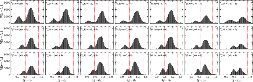
Figure 22: The $(g-i)_{o}$ histograms reflect all stars in each field with $i_{o}$ magnitudes falling between the limits shown in Figure 21. The two populations in each panel are the foreground main-sequence (blue group) and the bulge red clump stars (red group). Note that the blue main-sequence population shifts redward with increasing distance from the plane, which simultaneously decreases the color difference between the two groups. However, at higher latitudes the foreground sample is also more easily rejected by Gaia proper motions.

References

- Alam et al. (2015) Alam S., et al., 2015, ApJS, 219, 12
- Alves (2000) Alves D. R., 2000, ApJ, 539, 732
- Alves-Brito et al. (2010) Alves-Brito A., Meléndez J., Asplund M., Ramírez I., Yong D., 2010, Astronomy and Astrophysics, 513, A35
- Arentsen et al. (2020) Arentsen A., et al., 2020, MNRAS, 491, L11
- Athanassoula (2005) Athanassoula E., 2005, MNRAS, 358, 1477
- Athanassoula et al. (2017) Athanassoula E., Rodionov S. A., Prantzos N., 2017, MNRAS, 467, L46
- Babusiaux (2016) Babusiaux C., 2016, Publications of the Astronomical Society of Australia, 33, e026
- Babusiaux et al. (2010) Babusiaux C., et al., 2010, Astronomy and Astrophysics, 519, A77
- Ballero et al. (2007) Ballero S. K., Matteucci F., Origlia L., Rich R. M., 2007, A&A, 467, 123
- Barbuy et al. (2018) Barbuy B., Chiappini C., Gerhard O., 2018, Annual Review of Astronomy and Astrophysics, 56, 223
- Bensby et al. (2013) Bensby T., et al., 2013, Astronomy and Astrophysics, 549, A147
- Bensby et al. (2014) Bensby T., Feltzing S., Oey M. S., 2014, A&A, 562, A71
- Bensby et al. (2017) Bensby T., et al., 2017, A&A, 605, A89
- Boeche et al. (2014) Boeche C., et al., 2014, A&A, 568, A71
- Bovy et al. (2019) Bovy J., Leung H. W., Hunt J. A. S., Mackereth J. T., García-Hernández D. A., Roman-Lopes A., 2019, MNRAS, 490, 4740
- Cao et al. (2013) Cao L., Mao S., Nataf D., Rattenbury N. J., Gould A., 2013, MNRAS, 434, 595
- Catchpole et al. (2016) Catchpole R. M., Whitelock P. A., Feast M. W., Hughes S. M. G., Irwin M., Alard C., 2016, MNRAS, 455, 2216
- Chambers et al. (2016) Chambers K. C., et al., 2016, arXiv e-prints, p. arXiv:1612.05560
- Choi et al. (2016) Choi J., Dotter A., Conroy C., Cantiello M., Paxton B., Johnson B. D., 2016, ApJ, 823, 102
- Clarke et al. (2019) Clarke J. P., Wegg C., Gerhard O., Smith L. C., Lucas P. W., Wylie S. M., 2019, MNRAS, 489, 3519
- Clarkson et al. (2008) Clarkson W., et al., 2008, The Astrophysical Journal, 684, 1110
- Clarkson et al. (2018) Clarkson W. I., et al., 2018, ApJ, 858, 46
- Cole et al. (2000) Cole S., Lacey C. G., Baugh C. M., Frenk C. S., 2000, MNRAS, 319, 168
- Combes et al. (1990) Combes F., Debbasch F., Friedli D., Pfenniger D., 1990, A&A, 233, 82
- Côté et al. (2017) Côté B., O’Shea B. W., Ritter C., Herwig F., Venn K. A., 2017, ApJ, 835, 128
- Debattista et al. (2017) Debattista V. P., Ness M., Gonzalez O. A., Freeman K., Zoccali M., Minniti D., 2017, MNRAS, 469, 1587
- Dékány et al. (2013) Dékány I., Minniti D., Catelan M., Zoccali M., Saito R. K., Hempel M., Gonzalez O. A., 2013, The Astrophysical Journal, 776, L19
- Dekel & Burkert (2014) Dekel A., Burkert A., 2014, MNRAS, 438, 1870
- Di Matteo et al. (2014) Di Matteo P., et al., 2014, A&A, 567, A122
- Di Matteo et al. (2015) Di Matteo P., et al., 2015, A&A, 577, A1
- Di Matteo et al. (2019) Di Matteo P., Fragkoudi F., Khoperskov S., Ciambur B., Haywood M., Combes F., Gómez A., 2019, A&A, 628, A11
- Duong et al. (2019a) Duong L., Asplund M., Nataf D. M., Freeman K. C., Ness M., Howes L. M., 2019a, Monthly Notices of the Royal Astronomical Society, 486, 3586
- Duong et al. (2019b) Duong L., Asplund M., Nataf D. M., Freeman K. C., Ness M., 2019b, MNRAS, 486, 5349
- Eggen et al. (1962) Eggen O. J., Lynden-Bell D., Sandage A. R., 1962, ApJ, 136, 748
- Elmegreen et al. (2008) Elmegreen B. G., Bournaud F., Elmegreen D. M., 2008, ApJ, 688, 67
- Erwin et al. (2015) Erwin P., et al., 2015, MNRAS, 446, 4039
- Erwin et al. (2021) Erwin P., et al., 2021, MNRAS, 502, 2446
- Ferraro et al. (2009) Ferraro F. R., et al., 2009, Nature, 462, 483
- Ferraro et al. (2016) Ferraro F. R., Massari D., Dalessandro E., Lanzoni B., Origlia L., Rich R. M., Mucciarelli A., 2016, The Astrophysical Journal, 828, 75
- Ferraro et al. (2021) Ferraro F. R., et al., 2021, Nature Astronomy, 5, 311
- Fisher & Drory (2016) Fisher D. B., Drory N., 2016, An Observational Guide to Identifying Pseudobulges and Classical Bulges in Disc Galaxies. p. 41, doi:10.1007/978-3-319-19378-6_3
- Flaugher et al. (2015) Flaugher B., et al., 2015, AJ, 150, 150
- Fragkoudi et al. (2018) Fragkoudi F., Di Matteo P., Haywood M., Schultheis M., Khoperskov S., Gómez A., Combes F., 2018, A&A, 616, A180
- Freeman et al. (2013) Freeman K., et al., 2013, Monthly Notices of the Royal Astronomical Society, 428, 3660
- Fulbright et al. (2006) Fulbright J. P., McWilliam A., Rich R. M., 2006, ApJ, 636, 821
- Fulbright et al. (2007) Fulbright J. P., McWilliam A., Rich R. M., 2007, The Astrophysical Journal, 661, 1152
- Gaia Collaboration et al. (2021) Gaia Collaboration et al., 2021, A&A, 649, A1
- García Pérez et al. (2013) García Pérez A. E., et al., 2013, ApJ, 767, L9
- Gennaro et al. (2015) Gennaro M., Tchernyshyov K., Brown T. M., Gordon K. D., 2015, ApJ, 808, 45
- Gilmore et al. (2012) Gilmore G., et al., 2012, The Messenger, 147, 25
- Girardi & Salaris (2001) Girardi L., Salaris M., 2001, MNRAS, 323, 109
- Gonzalez et al. (2011) Gonzalez O. A., et al., 2011, Astronomy and Astrophysics, 530, A54
- Gonzalez et al. (2012) Gonzalez O. A., Rejkuba M., Zoccali M., Valenti E., Minniti D., Schultheis M., Tobar R., Chen B., 2012, A&A, 543, A13
- Gonzalez et al. (2013) Gonzalez O. A., Rejkuba M., Zoccali M., Valent E., Minniti D., Tobar R., 2013, Astronomy and Astrophysics, 552, A110
- Gonzalez et al. (2015) Gonzalez O. A., Zoccali M., Debattista V. P., Alonso-García J., Valenti E., Minniti D., 2015, A&A, 583, L5
- Gonzalez et al. (2018) Gonzalez O. A., et al., 2018, MNRAS, 481, L130
- Grady et al. (2020) Grady J., Belokurov V., Evans N. W., 2020, MNRAS, 492, 3128
- Gravity Collaboration et al. (2019) Gravity Collaboration et al., 2019, A&A, 625, L10
- Grieco et al. (2012) Grieco V., Matteucci F., Pipino A., Cescutti G., 2012, A&A, 548, A60
- Griffith et al. (2021) Griffith E., et al., 2021, ApJ, 909, 77
- Hasselquist et al. (2020) Hasselquist S., et al., 2020, ApJ, 901, 109
- Hawkins et al. (2017) Hawkins K., Leistedt B., Bovy J., Hogg D. W., 2017, MNRAS, 471, 722
- Haywood et al. (2016) Haywood M., Di Matteo P., Snaith O., Calamida A., 2016, Astronomy and Astrophysics, 593, A82
- Hill et al. (2011) Hill V., et al., 2011, Astronomy and Astrophysics, 534, A80
- Hopkins et al. (2009) Hopkins P. F., Cox T. J., Younger J. D., Hernquist L., 2009, ApJ, 691, 1168
- Horta et al. (2021) Horta D., et al., 2021, MNRAS, 500, 1385
- Howard et al. (2009) Howard C. D., et al., 2009, The Astrophysical Journal, 702, L153
- Howes et al. (2014) Howes L. M., et al., 2014, MNRAS, 445, 4241
- Howes et al. (2016) Howes L. M., et al., 2016, MNRAS, 460, 884
- Howes et al. (2019) Howes L. M., Lindegren L., Feltzing S., Church R. P., Bensby T., 2019, A&A, 622, A27
- Ibata et al. (2017) Ibata R. A., et al., 2017, ApJ, 848, 128
- Ivezić et al. (2008) Ivezić Ž., et al., 2008, ApJ, 684, 287
- Johnson et al. (2011) Johnson C. I., Rich R. M., Fulbright J. P., Valenti E., McWilliam A., 2011, The Astrophysical Journal, 732, 108
- Johnson et al. (2013) Johnson C. I., Rich R. M., Kobayashi C., Kunder A., Pilachowski C. A., Koch A., de Propris R., 2013, The Astrophysical Journal, 765, 157
- Johnson et al. (2014) Johnson C. I., Rich R. M., Kobayashi C., Kunder A., Koch A., 2014, AJ, 148, 67
- Johnson et al. (2020) Johnson C. I., et al., 2020, MNRAS, 499, 2357
- Jönsson et al. (2017) Jönsson H., Ryde N., Schultheis M., Zoccali M., 2017, Astronomy and Astrophysics, 598, A101
- Joyce et al. (2022) Joyce M., Johnson C. I., Marchetti T., Rich R. M., Simion I., Bourke J., 2022, arXiv e-prints, p. arXiv:2205.07964
- Keller et al. (2007) Keller S. C., et al., 2007, Publ. Astron. Soc. Australia, 24, 1
- Kirby et al. (2011) Kirby E. N., Lanfranchi G. A., Simon J. D., Cohen J. G., Guhathakurta P., 2011, ApJ, 727, 78
- Kisku et al. (2021) Kisku S., et al., 2021, MNRAS, 504, 1657
- Koch et al. (2007) Koch A., Grebel E. K., Kleyna J. T., Wilkinson M. I., Harbeck D. R., Gilmore G. F., Wyse R. F. G., Evans N. W., 2007, AJ, 133, 270
- Kormendy & Kennicutt (2004) Kormendy J., Kennicutt Robert C. J., 2004, Annual Review of Astronomy and Astrophysics, 42, 603
- Kuijken & Rich (2002) Kuijken K., Rich R. M., 2002, AJ, 124, 2054
- Kunder et al. (2012) Kunder A., et al., 2012, The Astronomical Journal, 143, 57
- Kunder et al. (2016) Kunder A., et al., 2016, The Astrophysical Journal, 821, L25
- Kunder et al. (2019) Kunder A., et al., 2019, The Astrophysical Journal, 877, L17
- Kunder et al. (2020) Kunder A., et al., 2020, AJ, 159, 270
- Laney et al. (2012) Laney C. D., Joner M. D., Pietrzyński G., 2012, MNRAS, 419, 1637
- Larson (1974) Larson R. B., 1974, MNRAS, 166, 585
- Lee et al. (2019) Lee Y.-W., Kim J. J., Johnson C. I., Chung C., Jang S., Lim D., Kang Y., 2019, The Astrophysical Journal, 878, L2
- Li & Shen (2012) Li Z.-Y., Shen J., 2012, ApJ, 757, L7
- Li & Shen (2015) Li Z.-Y., Shen J., 2015, ApJ, 815, L20
- Lim et al. (2021a) Lim D., et al., 2021a, A&A, 647, A34
- Lim et al. (2021b) Lim D., et al., 2021b, ApJ, 907, 47
- López-Corredoira (2017) López-Corredoira M., 2017, ApJ, 836, 218
- López-Corredoira et al. (2005) López-Corredoira M., Cabrera-Lavers A., Gerhard O. E., 2005, A&A, 439, 107
- Lucertini et al. (2021) Lucertini F., Monaco L., Caffau E., Bonifacio P., Mucciarelli A., 2021, arXiv e-prints, p. arXiv:2109.06216
- Lucey et al. (2021) Lucey M., et al., 2021, MNRAS, 501, 5981
- Majewski et al. (2017) Majewski S. R., et al., 2017, The Astronomical Journal, 154, 94
- Marchetti et al. (2022) Marchetti T., et al., 2022, arXiv e-prints, p. arXiv:2206.12817
- McWilliam & Zoccali (2010) McWilliam A., Zoccali M., 2010, The Astrophysical Journal, 724, 1491
- Meléndez et al. (2008) Meléndez J., et al., 2008, Astronomy and Astrophysics, 484, L21
- Minniti et al. (2010) Minniti D., et al., 2010, New Astronomy, 15, 433
- Mohammed et al. (2019) Mohammed S., Schiminovich D., Hawkins K., Johnson B., Wang D., Hogg D. W., 2019, ApJ, 872, 95
- Mould (1984) Mould J. R., 1984, PASP, 96, 773
- Nandakumar et al. (2020) Nandakumar G., et al., 2020, arXiv e-prints, p. arXiv:2011.02783
- Nataf et al. (2010) Nataf D. M., Udalski A., Gould A., Fouqué P., Stanek K. Z., 2010, The Astrophysical Journal, 721, L28
- Nataf et al. (2013) Nataf D. M., Gould A. P., Pinsonneault M. H., Udalski A., 2013, ApJ, 766, 77
- Nataf et al. (2014) Nataf D. M., Cassisi S., Athanassoula E., 2014, MNRAS, 442, 2075
- Nataf et al. (2021) Nataf D. M., Cassisi S., Casagrande L., Yuan W., Riess A. G., 2021, ApJ, 910, 121
- Ness & Lang (2016) Ness M., Lang D., 2016, The Astronomical Journal, 152, 14
- Ness et al. (2013a) Ness M., et al., 2013a, Monthly Notices of the Royal Astronomical Society, 430, 836
- Ness et al. (2013b) Ness M., et al., 2013b, Monthly Notices of the Royal Astronomical Society, 432, 2092
- Ness et al. (2014) Ness M., Debattista V. P., Bensby T., Feltzing S., Roškar R., Cole D. R., Johnson J. A., Freeman K., 2014, The Astrophysical Journal, 787, L19
- Onozato et al. (2019) Onozato H., Ita Y., Nakada Y., Nishiyama S., 2019, MNRAS, 486, 5600
- Origlia et al. (2011) Origlia L., et al., 2011, ApJ, 726, L20
- Ortolani et al. (1995) Ortolani S., Renzini A., Gilmozzi R., Marconi G., Barbuy B., Bica E., Rich R. M., 1995, Nature, 377, 701
- Palacios et al. (2010) Palacios A., Gebran M., Josselin E., Martins F., Plez B., Belmas M., Lèbre A., 2010, A&A, 516, A13
- Paterson et al. (2020) Paterson D., Coleman B., Gordon C., 2020, MNRAS, 499, 1937
- Peletier et al. (2007) Peletier R. F., et al., 2007, MNRAS, 379, 445
- Pietrukowicz et al. (2015) Pietrukowicz P., et al., 2015, The Astrophysical Journal, 811, 113
- Plevne et al. (2020) Plevne O., Önal Taş Ö., Bilir S., Seabroke G. M., 2020, ApJ, 893, 108
- Queiroz et al. (2020) Queiroz A. B. A., et al., 2020, arXiv e-prints, p. arXiv:2007.12915
- Renzini et al. (2018) Renzini A., et al., 2018, The Astrophysical Journal, 863, 16
- Rich (1990) Rich R. M., 1990, ApJ, 362, 604
- Rich et al. (2007a) Rich R. M., Reitzel D. B., Howard C. D., Zhao H., 2007a, The Astrophysical Journal, 658, L29
- Rich et al. (2007b) Rich R. M., Origlia L., Valenti E., 2007b, ApJ, 665, L119
- Rich et al. (2012) Rich R. M., Origlia L., Valenti E., 2012, The Astrophysical Journal, 746, 59
- Rich et al. (2020) Rich R. M., et al., 2020, MNRAS, 499, 2340
- Robin et al. (2003) Robin A. C., Reylé C., Derrière S., Picaud S., 2003, A&A, 409, 523
- Rojas-Arriagada et al. (2014) Rojas-Arriagada A., et al., 2014, A&A, 569, A103
- Rojas-Arriagada et al. (2017) Rojas-Arriagada A., et al., 2017, Astronomy and Astrophysics, 601, A140
- Rojas-Arriagada et al. (2020) Rojas-Arriagada A., et al., 2020, MNRAS, 499, 1037
- Ruiz-Dern et al. (2018) Ruiz-Dern L., Babusiaux C., Arenou F., Turon C., Lallement R., 2018, A&A, 609, A116
- Saha et al. (2019) Saha A., et al., 2019, ApJ, 874, 30
- Saito et al. (2011) Saito R. K., Zoccali M., McWilliam A., Minniti D., Gonzalez O. A., Hill V., 2011, The Astronomical Journal, 142, 76
- Savino et al. (2020) Savino A., Koch A., Prudil Z., Kunder A., Smolec R., 2020, arXiv e-prints, p. arXiv:2006.12507
- Schiavon et al. (2017) Schiavon R. P., et al., 2017, MNRAS, 465, 501
- Schlesinger et al. (2014) Schlesinger K. J., et al., 2014, ApJ, 791, 112
- Schönrich & McMillan (2017) Schönrich R., McMillan P. J., 2017, MNRAS, 467, 1154
- Schultheis et al. (2019) Schultheis M., Rich R. M., Origlia L., Ryde N., Nandakumar G., Thorsbro B., Neumayer N., 2019, Astronomy and Astrophysics, 627, A152
- Shen et al. (2010) Shen J., Rich R. M., Kormendy J., Howard C. D., De Propris R., Kunder A., 2010, The Astrophysical Journal, 720, L72
- Simion et al. (2017) Simion I. T., Belokurov V., Irwin M., Koposov S. E., Gonzalez-Fernandez C., Robin A. C., Shen J., Li Z. Y., 2017, MNRAS, 471, 4323
- Simion et al. (2021) Simion I. T., Shen J., Koposov S. E., Ness M., Freeman K., Bland-Hawthorn J., Lewis G. F., 2021, MNRAS, 502, 1740
- Sit & Ness (2020) Sit T., Ness M. K., 2020, ApJ, 900, 4
- Soszyński et al. (2014) Soszyński I., et al., 2014, Acta Astronomica, 64, 177
- Soto et al. (2007) Soto M., Rich R. M., Kuijken K., 2007, The Astrophysical Journal, 665, L31
- Soto et al. (2012) Soto M., Kuijken K., Rich R. M., 2012, A&A, 540, A48
- Stanek et al. (1994) Stanek K. Z., Mateo M., Udalski A., Szymanski M., Kaluzny J., Kubiak M., 1994, ApJ, 429, L73
- Surot et al. (2019) Surot F., et al., 2019, Astronomy and Astrophysics, 623, A168
- Tacchella et al. (2016) Tacchella S., Dekel A., Carollo C. M., Ceverino D., DeGraf C., Lapiner S., Mandelker N., Primack J. R., 2016, MNRAS, 458, 242
- Valenti et al. (2013) Valenti E., Zoccali M., Renzini A., Brown T. M., Gonzalez O. A., Minniti D., Debattista V. P., Mayer L., 2013, Astronomy and Astrophysics, 559, A98
- Walker & Terndrup (1991) Walker A. R., Terndrup D. M., 1991, ApJ, 378, 119
- Wegg & Gerhard (2013) Wegg C., Gerhard O., 2013, Monthly Notices of the Royal Astronomical Society, 435, 1874
- Wylie et al. (2021) Wylie S. M., Gerhard O. E., Ness M. K., Clarke J. P., Freeman K. C., Bland-Hawthorn J., 2021, arXiv e-prints, p. arXiv:2106.14298
- Zasowski et al. (2019) Zasowski G., et al., 2019, The Astrophysical Journal, 870, 138
- Zhao et al. (1994) Zhao H., Spergel D. N., Rich R. M., 1994, AJ, 108, 2154
- Zoccali et al. (2003) Zoccali M., et al., 2003, Astronomy and Astrophysics, 399, 931
- Zoccali et al. (2006) Zoccali M., et al., 2006, Astronomy and Astrophysics, 457, L1
- Zoccali et al. (2008) Zoccali M., Hill V., Lecureur A., Barbuy B., Renzini A., Minniti D., Gómez A., Ortolani S., 2008, Astronomy and Astrophysics, 486, 177
- Zoccali et al. (2014) Zoccali M., et al., 2014, Astronomy and Astrophysics, 562, A66
- Zoccali et al. (2017) Zoccali M., et al., 2017, A&A, 599, A12
- Zolotov et al. (2015) Zolotov A., et al., 2015, MNRAS, 450, 2327
- Zou et al. (2016) Zou H., et al., 2016, AJ, 151, 37